


Abstract
This study develops and analyzes a four-state nonlinear policy–feedback dynamical system that couples a system stressor, an accumulated burden, a signed mitigation–response variable, and a signed policy-pressure variable. The proposed model represents governance response through a smooth threshold-centered feedback mechanism, in which the policy-pressure dynamics depend continuously on the deviation of the stressor from a prescribed reference threshold. Unlike reduced-order formulations with purely exogenous interventions, the present framework generates endogenous interactions among stress accumulation, burden evolution, mitigation response, and policy adjustment. The qualitative analysis establishes local well-posedness in the admissible phase domain, conditional nonnegativity of the accumulated burden, and boundedness of trajectories on admissible intervals. An autonomous effective system is then derived to characterize quasi-stationary mean behavior of the periodically forced dynamics. For this effective system, local stability is investigated using Gershgorin estimates and Routh–Hurwitz criteria, leading to explicit analytical conditions for local asymptotic stability and a critical policy-responsiveness threshold associated with possible Hopf-type oscillatory transitions. The analysis highlights the stabilizing role of mitigation damping and cubic saturation in regulating the feedback loop. To approximate the nonlinear system, a Physics-Informed Neural Network (PINN) surrogate is constructed by embedding the governing equations into a differentiable residual loss while enforcing the initial conditions analytically. The accumulated burden is represented through an admissible neural-network ansatz to preserve the well-definedness of the logarithmic coupling term, while the mitigation–response and policy-pressure variables remain signed in accordance with the model formulation. Numerical validation against reference ode45 solutions across two governance regimes shows maximum absolute errors of order , indicating that the PINN provides a reliable differentiable surrogate for the coupled policy–feedback dynamics. The resulting framework offers a foundation for future inverse modeling, parameter estimation, and data-assimilation studies involving policy responsiveness, intervention thresholds, and burden- suppression effects.
Keywords:
Physics-Informed Neural Networks; policy–feedback dynamics; nonlinear systems; mitigation modeling; threshold-centered policy feedback MSC:
34A34; 34D20; 65L05; 68T07
1. Introduction
Many socio-technical systems evolve under the combined influence of physical stressors, accumulated demand or burden, mitigation capacity, and governance interventions. Prominent examples include urban heat management, energy demand regulation, pollution exposure mitigation, and infrastructure stress control. In urban environments, heat indices exceeding 35– are commonly used as activation thresholds for heat-action plans, while electrical grids experience critical stress when peak demand approaches 85– of installed capacity [1,2]. These systems are characterized by nonlinear feedback in which policy responses are triggered by stress exceedance, yet are often delayed, weakened, or reversed due to institutional inertia, competing priorities, or socio-economic constraints. In each of these domains, four interacting quantities govern system evolution: a measurable stressor index (heat level, pollutant concentration, or grid demand), an accumulated burden that integrates exposure over time (population health impact or cumulative infrastructure overload), a mitigation effort variable (cooling deployment, emission curtailment, or demand response), and a governance signal that activates, intensifies, or retreats in response to stress exceedance. Capturing the bidirectional and threshold-sensitive nature of this governance signal within a compact mathematical framework motivates the four-state structure proposed in this work. Reduced-order dynamical models have long been employed to study such systems because of their analytical transparency and computational efficiency [3,4]. In the context of urban systems and energy management, low-dimensional models have been used to describe aggregate demand growth, mitigation strategies, and long-term stability [5,6]. However, in most existing frameworks, policy interventions are imposed exogenously, for example, through fixed mitigation schedules or predefined control trajectories. As a result, these models cannot capture adaptive governance behavior, threshold-activated responses, or policy relaxation mechanisms that are frequently observed in practice. Empirical studies of governance in complex systems demonstrate that policy action is often reactive rather than proactive, activating only after system stress exceeds critical thresholds [7]. Furthermore, policy influence is not necessarily monotonic: mitigation efforts may intensify, stagnate, or retreat depending on political, economic, and institutional conditions. Accurately representing this bidirectional and state-dependent behavior within a compact mathematical framework remains an open challenge in reduced-order modeling of policy-sensitive systems. Existing reduced-order models of policy-sensitive socio-technical systems typically operate with two or three state variables. Two-state formulations couple a stressor directly to a single response variable, precluding any representation of burden accumulation as a distinct slow stock [3,4]. Three-state extensions introduce either an accumulated burden or a mitigation capacity but invariably treat the governance component as an exogenous input or a fixed parameter schedule [5,6]. Consequently, none of these frameworks can simultaneously represent the following four empirically documented phenomena within a single coherent dynamical system:
- (i)
- Threshold-triggered governance activation, in which policy pressure builds only after the stressor exceeds a prescribed critical level;
- (ii)
- Bidirectional policy behavior, encompassing both active regulatory enforcement and institutional relaxation or policy reversal;
- (iii)
- Nonlinear saturation of mitigation capacity, capturing effort fatigue and bounded response authority under sustained stress;
- (iv)
- Saturating burden-stress coupling, reflecting diminishing marginal amplification as accumulated burden grows large.
The four-state structure proposed here is therefore the minimal formulation capable of capturing all four phenomena within a single unified dynamical framework. Reducing the system by one state, for instance, by collapsing the governance variable into the mitigation variable or the accumulated burden into the instantaneous stressor, eliminates the ability to represent policy relaxation independently of mitigation decay or long-term burden accumulation independently of short-term stress fluctuations. These distinctions are central to adaptive governance theory and empirically documented in the management of complex socio-technical systems [7]. It is also important to note at the outset that the threshold-driven policy mechanism proposed in this work, in which policy pressure responds proportionally to stress exceedance and decays over time, is structurally related to classical proportional integral control in the engineering literature. We acknowledge this connection explicitly. However, the novelty of the proposed formulation does not reside in the policy equation viewed in isolation but rather in the closed-loop nonlinear system behavior that emerges when the policy variable is simultaneously coupled to burden accumulation, mitigation deployment, and a nonlinearly forced stressor. In particular, the policy variable is allowed to take both positive and negative values, enabling the model to represent not only active governance enforcement but also institutional relaxation, policy reversal, and rebound dynamics behavioral modes that are well-documented empirically [7] but absent from standard nonnegative control formulations. In addition, threshold-based intervention rules have been widely used to represent state-dependent treatment, control, or governance responses in nonlinear dynamical systems. Recent work on non-smooth threshold strategies has shown that such mechanisms can substantially alter stability, transition behavior, and long-term system outcomes [8]. Also, the need for adaptive response mechanisms is central in nonlinear networked control systems, where data-driven resilient control strategies have been developed to maintain performance under external disruptions [9]. Motivated by this gap, the present study introduces a new low-dimensional nonlinear policy–feedback dynamical model that explicitly couples four interacting state variables: a system stressor, an accumulated burden, a mitigation effort, and a signed policy-pressure index. The proposed formulation incorporates an endogenous, threshold-activated policy mechanism that responds dynamically to stress exceedance and feeds back into both mitigation deployment and burden accumulation. Nonlinear saturation of mitigation capacity and dissipation effects are included to ensure realistic bounded behavior and long-term stability. This structure enables systematic investigation of how the timing, strength, and persistence of policy intervention shape system trajectories under different governance regimes. Solving such tightly coupled nonlinear systems pose challenges for classical numerical methods, particularly in the presence of activation thresholds, stiff feedback, and inequality constraints on state variables.
In recent years, Physics-Informed Neural Networks (PINNs) have emerged as a powerful computational paradigm for solving differential equations by embedding governing physical laws directly into the training process of neural networks. Originally introduced by Raissi et al. [10], PINNs construct a unified loss function that penalizes violations of differential equations, initial and boundary conditions, and auxiliary constraints. Their mesh-free formulation and use of automatic differentiation enable accurate evaluation of derivatives and flexible handling of nonlinear dynamics without explicit time discretization. Extensive research has demonstrated the effectiveness of PINNs across a wide range of scientific and engineering applications. Karniadakis et al. [11] provided a comprehensive overview of PINN methodologies and their applications to forward and inverse problems. Cuomo et al. [12] illustrated the use of PINNs in multiphysics environments, highlighting their strong generalization capability under limited data availability conditions. Theoretical investigations by Ghattas et al. [13] examined the mathematical foundations of learning differential equations, emphasizing stability and convergence properties of physics-informed approaches. Extensions of PINNs have been proposed for stochastic systems [14], fractional-order dynamics [15], and inverse geophysical problems [16]. Methodological advancements such as adaptive loss weighting [17] and domain decomposition strategies [18] have further improved robustness and scalability. Operator-learning frameworks, including DeepONets [19] and XPINNs [20], have broadened the applicability of the physics-informed paradigm. Building on these foundations, subsequent work established systematic software frameworks for the PINN-based solution of differential Equations [21], while gradient balancing strategies [22] and early neural network approaches to differential Equations [23] further consolidated the methodological basis of the field. Recent extensions of physics-informed learning, including physics-informed extreme learning machines for interface and moving-boundary problems [24], further demonstrate the flexibility of embedding governing equations directly into trainable surrogate models. Deep-learning surrogates have recently been used to predict nonlinear dynamic stress–strain responses in complex materials and geotechnical systems [25], illustrating the growing role of data-driven models in approximating stress-driven transient dynamics. In this work, we use the standard PINN formulation because the governing system is a low-dimensional smooth ODE system while retaining the differentiable structure needed for future inverse modeling. Applications of PINNs to epidemiological and biological dynamical systems [26,27] demonstrate their suitability for low-dimensional nonlinear ODE systems beyond classical physics, while inverse problem formulations [28,29] establish the PINN framework as a principled tool for parameter identification and data assimilation in systems with partially unknown governing parameters. Despite these advances, PINNs have not previously been applied to generic policy–feedback dynamical systems that incorporate threshold-driven governance, signed policy-pressure dynamics, and nonlinear mitigation saturation within a unified low-dimensional framework.
This paper addresses these limitations by developing the model described above and validating it computationally through a PINN framework. The bidirectional coupling between policy pressure, burden accumulation, and mitigation effort enables systematic investigation of how policy timing, responsiveness, and persistence shape system trajectories in stress-driven socio-technical environments. To solve the resulting nonlinear and tightly coupled system, a Physics-Informed Neural Network (PINN) framework is constructed, embedding the governing differential equations and physical constraints directly into the loss function. The PINN-based solutions are validated against high-accuracy reference trajectories obtained using the classical ode45 solver, demonstrating excellent agreement across all state variables with typical errors remaining below . It is important to clarify that for low-dimensional smooth ordinary differential systems with fully known parameters, classical numerical solvers such as ode45 provide highly efficient and accurate forward simulations. The motivation for adopting a Physics-Informed Neural Network (PINN) in the present study is therefore not computational acceleration of deterministic time integration. Rather, the PINN framework provides a globally differentiable surrogate representation of the coupled nonlinear policy–feedback dynamics. This differentiable structure enables seamless integration with parameter estimation, inverse modeling, and hybrid data-assimilation extensions, in which unknown policy responsiveness coefficients, threshold levels, or mitigation effectiveness parameters may be learned directly from sparse or noisy observations. Consequently, the PINN formulation should be viewed as a flexible computational infrastructure for future inverse and data-driven policy–feedback analysis, rather than as a replacement for classical time-stepping schemes in purely forward deterministic settings. In addition, two distinct governance regimes are examined: a baseline proportional-response configuration and a strong early-intervention regime. This scenario-based analysis reveals the critical role of timely and sustained policy activation in limiting stress amplification, reducing accumulated burden, and promoting overall system stabilization. The main contributions of this study are summarized as follows:
- A new four-state nonlinear policy–feedback dynamical model is introduced, coupling system stress, accumulated burden, mitigation effort, and a signed policy-pressure variable through an endogenous threshold-driven governance mechanism.
- A Physics-Informed Neural Network (PINN) formulation is constructed that enforces initial conditions analytically and embeds the full nonlinear policy–feedback structure within a differentiable surrogate representation.
- Beyond forward simulation, the proposed PINN framework is extended to a parameter identification setting, demonstrating its capability for inverse modeling in policy-sensitive dynamical systems.
- A comparative analysis of two governance regimes (baseline and strong early intervention) illustrates how policy timing and responsiveness shape long-term stability.
- The framework establishes a computational foundation suitable for future extensions involving parameter learning, uncertainty quantification, sparse observational data, and hybrid data-driven governance modeling.
To substantiate the novelty claims made above, Table 1 provides a concise structured comparison of the proposed four-state framework with the most relevant prior reduced-order models for socio-technical policy–feedback systems. For each prior model, the table identifies the number of state variables, the treatment of the governance component, the presence or absence of threshold activation, the sign of the policy variable, and whether nonlinear saturation of the mitigation or response capacity is included. The comparison is organized around the four phenomena identified above as absent from existing frameworks.
Table 1.
Structured comparison of the proposed four-state policy–feedback model with representative prior reduced-order models for socio-technical systems.
The table makes precise what the verbal claims in the Introduction assert. The key structural distinction is that in every prior reduced-order model identified, the governance or policy component enters as an exogenous input a prescribed forcing function or fixed scenario parameter rather than as a dynamical state variable governed by its own differential equation coupled endogenously to the stressor. As a consequence, none of the prior models can exhibit threshold-triggered governance activation, signed policy reversal, or the interplay between policy decay and mitigation saturation that determines the stable-to-oscillatory transition. The four-state structure proposed here is the minimal extension that makes all four phenomena simultaneously representable within a single analytically tractable and computationally validated dynamical framework.
The remainder of this paper is organized as follows. Section 2 presents the mathematical formulation of the policy–feedback model. Section 3 provides the qualitative analysis of the model along with bifurcation analysis. Section 4 describes the Physics-Informed Neural Network methodology and training strategy. Section 5 reports numerical simulations and physical interpretation for the two governance regimes. Section 6 concludes the study and outlines directions for future research.
2. Nonlinear Policy-Feedback Dynamical System
In this section, we formulate a nonlinear policy–feedback model describing the interaction between an evolving system stressor, its accumulated burden, mitigation effort, and policy pressure. The proposed model integrates low-dimensional structure while incorporating nonlinear feedback mechanisms suitable for different policy-driven systems.The dynamics of the system are governed by the following system
where represents the system stressor, denotes the accumulated burden, corresponds to a signed mitigation–response state, and represents signed policy pressure. Positive values of describe effective mitigation activity, whereas negative values describe response deficit or relaxation relative to a neutral baseline. The initial conditions can be in the following form
In the simulations reported in Section 5, we use the baseline initial condition
This choice represents an initially neutral state and is adopted for illustration. Other initial conditions may lead to quantitatively different transients, although the boundedness and local stability conclusions derived below remain governed by the same dissipative structure. The nonlinear logarithmic term in the first equation of system (1) captures saturation effects in the influence of accumulated burden on the stressor, while the cubic term in the mitigation equation ensures bounded response dynamics. The periodic forcing term represents external cyclical influences. In addition, the parameter a denotes the relaxation rate of the stressor variable, while quantifies the nonlinear effect of the accumulated burden on stress amplification. The parameter represents the effectiveness of mitigation effort in reducing system stress. The parameters and k characterize the baseline input and its decay over time, whereas governs the removal or dissipation of the accumulated burden. Policy-related effects are controlled by the parameters , , and , which describe the influence of policy pressure on burden accumulation, mitigation activation, and policy responsiveness, respectively. The parameters and account for decay and saturation in mitigation effort, while represents the relaxation rate of policy pressure. The threshold determines the stress level at which policy intervention is triggered. Table 2 summarizes the definitions of the state variables, while Table 3 provides the definitions of the model parameters. In addition, Figure 1 illustrates the schematic diagram of the interactions among the different states of the proposed model.
Table 2.
Definitions of the state variables in the proposed policy–feedback system.
Table 3.
Definitions of the model parameters used in the proposed policy–feedback system.
Figure 1.
Schematic diagram of the proposed policy–feedback system, including the external forcing term acting on the stressor state .
Remark 1.
The proposed system is locally Lipschitz-continuous in all state variables for admissible values , ensuring the existence and uniqueness of solutions. Moreover, the presence of dissipative terms , , , , and guarantees bounded trajectories for all state variables with finite inputs. In particular, the cubic damping term in the mitigation equation prevents unbounded growth of , while the logarithmic forcing term introduces saturation effects that limit stress amplification. We further clarify the relationship between the policy-pressure equation and classical control theory. The governing equation for ,
is, in isolation, a linear first-order filter on the threshold-error signal , structurally analogous to the integral action of a proportional integral (PI) controller in classical control theory. We acknowledge this explicitly. However, the novelty of the present formulation resides not in this equation alone but in the closed-loop nonlinear dynamics that emerge when is embedded within the full four-state coupled system. Four features distinguish this framework from a standard PD or PI control architecture applied to a linear plant:
- (i)
- Dual-channel policy coupling. The policy variable acts simultaneously on two state equations: it suppresses burden accumulation through the factor in the C-equation and drives mitigation deployment through the term in the U-equation. Standard PD controllers regulate a single output channel; the present formulation couples policy pressure to both a slow burden stock and a mitigation effort variable concurrently.
- (ii)
- Nonlinear mediation of control authority. The mitigation equation introduces cubic saturation that fundamentally bounds the effective control authority of . The resulting input–output map from policy pressure to mitigation effort is nonlinear and exhibits saturation and fatigue effects that are absent from any linear control formulation.
- (iii)
- Signed policy variable admitting relaxation dynamics. Unlike a nonnegative actuator signal in standard control design, is deliberately allowed to take negative values, representing institutional inertia, competing socio-economic priorities, or active policy reversal. This signed formulation enables the model to capture rebound and relaxation dynamics empirically observed in the governance of socio-technical systems [7], which cannot be represented by a standard unsigned controller.
- (iv)
- Nonlinear generation of the error signal. The logarithmic term in the stressor equation means that the effective signal driving is not a simple linear error but is shaped by a nonlinear, saturating burden history. This produces a closed feedback cascade in which burden nonlinearly amplifies stress, stress drives policy pressure, and policy pressure suppresses burden a structure qualitatively richer than a PD controller applied to a linear plant.
These features produce closed-loop system behaviors, including policy-induced burden suppression, mitigation saturation, and signed pressure oscillations that cannot be recovered from any standard linear control architecture operating on a single regulated output.
3. Qualitative Analysis of the Dynamical System
In this section, we investigate the fundamental dynamical properties of system (1), including equilibrium structure, local stability, and boundedness.
3.1. Positivity and Forward Invariance
In many applications motivating system (1), the accumulated burden is naturally interpreted as a nonnegative stock. In contrast, the present formulation deliberately treats the policy-pressure variable as signed. Consequently, the mitigation–response variable should also be interpreted as a signed response index rather than as a strictly nonnegative stock. Positive values of correspond to active mitigation deployment, while negative values describe response deficit, rebound, or relaxation relative to the neutral baseline. Therefore, the nonnegative orthant is not claimed to be globally forward-invariant for the full signed system. Instead, we establish conditional nonnegativity of and boundedness of the signed variables under admissible parameter regimes. We assume that on the time interval of interest,
so that the effective burden input factor satisfies . This condition permits the full range of positive policy pressure without restriction, while excluding only strongly negative policy values that would cause the burden input rate to become negative.
Theorem 1.
Let and suppose that
on the time interval under consideration. Then on that interval.
Proof.
From (1), satisfies
If , then , so the forcing term on the right-hand side is nonnegative. Hence, by the variation-of-constants formula,
Therefore remains nonnegative on the interval. □
Remark 2.
Because is signed, Equation
does not guarantee forward invariance of the half-line . Indeed, at the boundary ,
Thus, if , the vector field points toward . This is not a mathematical inconsistency but rather reflects the signed interpretation adopted in the present model: negative values of represent mitigation deficit or relaxation relative to the neutral baseline. Accordingly, the analysis below treats as a bounded signed response variable rather than as a strictly nonnegative stock.
Theorem 2.
Assume , , , and that the external forcing is either absent () or bounded in the sense that for all ,
Then for all .
Proof.
On the boundary , we have
Condition (4) implies ; hence, the vector field points inward at , and the nonnegative half-line for X is forward-invariant. □
Remark 3.
Because is signed, the equation
does not guarantee forward invariance of the half-line . Indeed, at ,
Thus, if , the vector field points toward . This behavior is consistent with the signed interpretation adopted in the present model: negative values of represent mitigation deficit, rebound, or relaxation relative to the neutral baseline. By contrast, the accumulated burden variable remains nonnegative under the sufficient condition
provided . If , the burden input factor becomes negative, and nonnegativity of is no longer guaranteed by the model structure alone. In that case, mathematical admissibility requires
so that the logarithmic term remains well-defined.
Remark 4.
Condition (3) is introduced as a sufficient condition to guarantee forward invariance of the nonnegative orthant for the stock and effort variables and in the theoretical analysis of Section 3. It is not intended as a modeling constraint that must be enforced in all regimes. The proposed framework deliberately allows to take both positive and negative values in order to capture the full range of policy behavior: positive values of correspond to active governance and regulatory enforcement, while negative values represent policy relaxation, institutional inertia, or competing socio-economic priorities. This signed formulation is a defining feature of the proposed model and distinguishes it from standard nonnegative control formulations. In the numerical simulations of Section 5, the trajectories of and remain nonnegative throughout. This is not merely an empirical observation: as established in Remark 3, when nonnegativity of holds analytically because , and when but the sufficient condition (3) is satisfied, providing the theoretical basis for the observed nonnegativity of throughout both simulations.
3.2. Boundedness of the Dynamical System
We now discuss the boundedness properties of system (1). Throughout this subsection, we assume
and we consider solutions in the admissible domain
so that the logarithmic term is well-defined. Since the vector field is locally Lipschitz-continuous in , every initial condition satisfying generates a unique local solution on a maximal interval .
The estimates below show that the state variables remain bounded on any admissible interval on which the solution stays uniformly separated from the logarithmic singularity .
Lemma 1.
For any initial condition and any bounded input , the signed mitigation–response variable remains bounded.
Proof.
From system (1),
Let
Then
Choose
If , then the cubic damping term dominates and
If , then
Thus, the interval
is absorbing for up to the initial value. Therefore,
and remains bounded. □
Lemma 2.
If is bounded, then is bounded.
Proof.
The C-equation in system (1) is linear:
Let
Then
By the variation-of-constants formula,
Hence,
Since
we obtain
Therefore, is bounded. □
Lemma 3.
Assume that and are bounded on an interval I, and suppose there exists a constant such that
Then is bounded on I.
Proof.
Assume that
Then the logarithmic argument satisfies
Therefore,
The X-equation can be written as
where
Using the bounds above,
By the variation-of-constants formula,
Hence,
Since
we obtain
Thus, is bounded on I. □
Lemma 4.
If is bounded, then is bounded.
Proof.
The P-equation in system (1) is linear:
If
then
Using the variation-of-constants formula,
Therefore,
Since
we obtain
Hence, is bounded. □
Theorem 3.
Let
be a solution of system (1) on an interval . Suppose that the solution remains uniformly admissible on I, that is, there exists such that
Then, on every bounded subinterval of I, all state variables remain bounded. Moreover, if the uniform admissibility condition holds for all and the corresponding bounds are uniform in time, then the solution exists globally and remains bounded for all .
Proof.
Local existence and uniqueness follow from the local Lipschitz continuity of the vector field in the admissible domain
Let be an arbitrary bounded interval. Since is continuous on , there exists
Using this local bound, Lemma 1 gives
Similarly, Lemma 2 gives
Because the solution is uniformly admissible on , there exists such that
Thus, Lemma 3 implies that is bounded on :
where
Finally, Lemma 4 yields
Therefore, all components remain bounded on the arbitrary bounded interval .
If the admissibility condition
holds for all , and the above bounds can be chosen uniformly in time, then the solution cannot either blow up or reach the logarithmic singularity in finite time. Hence, the maximal interval of existence is , and the solution remains globally bounded. □
Remark 5.
The theorem is deliberately stated under a uniform admissibility condition. This is necessary because the model contains the logarithmic term
which is singular at . Therefore, boundedness of alone is not sufficient; one must also ensure that remains separated from .
In particular, if and the policy-pressure variable satisfies
then the burden equation implies , and the logarithmic term remains well defined. Under such an admissible regime, the boundedness estimates above apply directly.
Remark 6.
The estimates above provide practical bounds of the form
together with analogous bounds for and . These estimates are useful for parameter sensitivity analysis and for justifying the numerical stability of the simulations on admissible time intervals.
3.3. Equilibrium Points
System (1) is non-autonomous because it contains the explicitly time-dependent terms and . Hence, classical equilibrium points of the original system, in the strict autonomous sense, do not exist. Nevertheless, useful analytical information about the long-term behavior can be obtained by considering suitable autonomous approximations. First, since , the exponentially decaying input satisfies
In addition, the periodic forcing has zero mean over one period. Therefore, the strictly averaged autonomous reference system is obtained by replacing by zero and by its mean value
The corresponding stationary equations are
Here, denotes the mean forcing contribution in the strictly averaged system. Since the periodic forcing has zero mean, we have . For the strictly averaged autonomous system with , the equilibrium conditions reduce as follows. From (6), one obtains
Substitution into (5) gives
and hence
Moreover, from (8),
Substituting (10) and (11) into (7) yields the scalar algebraic equation
Equation (12) determines the equilibrium stressor level of the strictly averaged autonomous system. Once is obtained, and follow from (10) and (11), respectively. It is important to note that the equilibrium of the strictly averaged system is generally a signed equilibrium. In particular, if , then (10) gives . This is not a contradiction in the present formulation because is interpreted as a signed mitigation–response variable. Positive values of represent active mitigation deployment, whereas negative values represent response deficit, relaxation, or rebound relative to the neutral baseline. For the original non-autonomous system, the persistent periodic forcing does not vanish as . Therefore, the long-time response should not be interpreted as convergence to a fixed equilibrium of the original system. Instead, the dissipative periodically forced system is expected to approach a bounded forced response, which may be viewed as oscillating around a representative mean state. To characterize the mean location of this periodically forced response, we introduce an effective constant forcing , estimated from the long-time average of the simulated trajectory. This quantity is not the time average of , which is zero. Rather, it is an empirical parameter used to define a representative quasi-stationary state of the forced system. The effective equilibrium is therefore defined by
From (14),
Furthermore, (13) and (16) give
and
Substitution of (17) and (18) into (15) gives the scalar effective-equilibrium equation
Thus, for a prescribed value of , the effective quasi-stationary stressor level is determined by (19), while and are then obtained from (17) and (18). The quantities , , , and used in the subsequent bifurcation, sensitivity, and local stability analyses are therefore interpreted as effective quasi-stationary mean values rather than exact equilibria of the original non-autonomous system. The stability analysis of Section 3.6 and the Routh–Hurwitz verification of Corollary 1 are applied to the Jacobian evaluated at these numerically identified effective equilibrium values. The resulting predictions are consistent with the observed bounded behavior and mean-state attraction of the simulated trajectories shown in Figures later in Section 5.
Remark 7.
The two external input terms in system (1) have qualitatively different asymptotic behaviors and therefore require separate interpretations. The decaying exponential satisfies
for any . Hence, its replacement by zero in the limiting system is an exact asymptotic statement. The periodic term , by contrast, does not vanish as . Replacing this term by its zero mean is not an asymptotic limit; rather, it is a time-averaging approximation. In a dissipative periodically forced system, the long-term response is generally not a fixed point but a bounded forced trajectory oscillating around a mean state. To illustrate the bounded influence of the periodic forcing, consider the linearized stressor equation around a quasi-stationary state:
Solving this linear forced equation gives a transient component together with a periodic steady-state component. Therefore,
After the exponentially decaying transient has vanished, the amplitude of the periodic forced component is bounded by
Thus, when is moderate, the periodically forced trajectory remains close to the effective quasi-stationary mean state after transients. This justifies the use of the effective equilibrium as a local analytical reference for the numerical trajectories.
3.4. Bifurcation Analysis
A central question in the analysis of policy-feedback systems is how variations in the policy responsiveness parameter affect the transition from locally stable effective-equilibrium behavior to oscillatory dynamics. In this subsection, we characterize this transition analytically through the eigenvalue structure of the Jacobian and derive explicit conditions on that determine the local qualitative regime of the effective autonomous system. The activation threshold does not enter the characteristic polynomial directly; rather, it affects stability indirectly through its influence on the effective equilibrium values, especially . The transition from stable to oscillatory dynamics can be understood through the following mechanism. When is small, policy pressure responds weakly to stress exceedance, and the dissipative terms , , and dominate, driving trajectories toward the effective equilibrium. As increases, the feedback loop
strengthens. Beyond a critical value , the local Routh–Hurwitz stability condition may be violated, and the effective equilibrium may lose stability through an oscillatory Hopf-type mechanism. The cubic saturation term plays a crucial role in this transition: by increasing the effective local damping
it limits the effective gain of the feedback loop and raises the instability threshold, thereby expanding the parameter region over which stable local behavior is observed. A necessary condition for a Hopf bifurcation at is that has a pair of purely imaginary eigenvalues with , with all other eigenvalues having strictly negative real parts, together with the usual nondegeneracy and transversality conditions [30]. Since with the stationary input approximation, the characteristic polynomial of factors as
where contributes the stable eigenvalue , and is the cubic polynomial arising from the subsystem:
with coefficients computed directly from :
By the Routh–Hurwitz criterion, all roots of have strictly negative real parts if and only if
Since , , and
for all positive parameters, local stability is governed by the third Routh–Hurwitz condition . Substituting (24)–(26) and writing
this condition reads
For a fixed effective equilibrium value , this condition can be rearranged to give the local instability threshold
At , the Routh–Hurwitz boundary is reached. Under the standard Hopf transversality and nondegeneracy assumptions, a complex conjugate pair of eigenvalues may cross the imaginary axis, indicating a Hopf-type transition. For , the local Routh–Hurwitz stability condition is violated, so the effective equilibrium is no longer guaranteed to be locally asymptotically stable. The critical value in (29) is an increasing function of , confirming that nonlinear mitigation saturation expands the stable parameter regime as the effective magnitude of grows.
Remark 8.
The critical policy responsiveness in (29) provides an explicit local analytical boundary separating stable from potentially oscillatory behavior in the subsystem. Three structural dependencies are immediately apparent from (29):
- (i)
- Policy decay rate : increases with δ. Faster decay of policy pressure acts as a natural stabilizer, effectively attenuating the feedback gain of the loop. Systems with rapid institutional relaxation therefore tolerate higher policy responsiveness without transitioning to oscillatory dynamics.
- (ii)
- Mitigation saturation : increases with the effective mitigation damping. The cubic saturation term is the central mechanism here: as grows, the effective linearized damping of the mitigation equation increases, raising and expanding the stable regime. This confirms that nonlinear saturation of mitigation capacity is not merely a boundedness device but plays a direct role in determining whether the policy–feedback loop stabilizes or destabilizes the local dynamics.
- (iii)
- Policy-to-mitigation coupling : decreases with ν. Stronger coupling between policy pressure and mitigation deployment amplifies the feedback loop and lowers the instability threshold, making the system more susceptible to oscillatory transitions at lower policy responsiveness.
The transition mechanism can be described as follows. For , all roots of the cubic characteristic polynomial in (23) have strictly negative real parts, and the effective equilibrium of the autonomous approximation is locally asymptotically stable. As ρ increases toward , the third Routh–Hurwitz quantity decreases toward zero. At , a complex conjugate pair of eigenvalues reaches the imaginary axis with nonzero imaginary part. If the Hopf transversality condition is satisfied, this signals the onset of oscillatory Hopf-type behavior. For ρ slightly above , the local equilibrium loses linear stability, and the nonlinear forced system may exhibit amplified oscillatory responses. The cubic saturation term may limit the growth of these oscillations, but global re-stabilization requires a separate nonlinear analysis. To connect this analysis to the simulated parameter regimes, we compute explicitly for both scenarios as a function of the mitigation equilibrium value :
- At ():Since , the local effective system operates well within the stable regime from the outset. This is consistent with the Routh–Hurwitz verification of Corollary 1, which confirms all stability conditions for Scenario I at the observed quasi-stationary value . The transient oscillatory behavior visible later is therefore attributed not to a local instability transition but to the nonlinear transient response of the system under the combined effect of periodic forcing and policy–feedback activation, as explained in Remark 7.
- Scenario II (, , , , , , ): With ,At ():Since , Scenario II also operates within the locally stable regime of the effective system. The more pronounced initial transient relative to Scenario I is explained by the stronger policy coupling , higher forcing amplitude , and lower policy decay rate , all of which amplify the nonlinear transient response before the system approaches its quasi-stationary mean state. The Routh–Hurwitz verification of Corollary 1 confirms local asymptotic stability at for this scenario.
These calculations establish three conclusions of direct policy relevance:
- (i)
- The instability threshold defined in (29) provides an explicit local analytical boundary: for , all eigenvalues of the subsystem have strictly negative real parts, and the effective equilibrium is locally asymptotically stable. At the critical boundary, a Hopf-type transition may occur if the required nondegeneracy and transversality conditions are satisfied.
- (ii)
- Both simulated scenarios satisfy , specifically for Scenario I and for Scenario II, confirming that both operate well within the locally stable regime from initialization. The transient oscillatory behavior observed later in Section 5 is a nonlinear transient response driven by periodic forcing and policy-feedback activation, not a consequence of proximity to the local instability boundary.
- (iii)
- The instability threshold increases with the policy decay rate δ, the mitigation decay rate μ, and the saturation coefficient ζ, and decreases with the policy-to-mitigation coupling ν and the mitigation-to-stressor coupling χ. This confirms that the cubic saturation term and rapid policy decay are primary structural stabilizers of the local effective system, expanding the range of admissible policy responsiveness ρ for which stable governance dynamics are predicted.
Threshold Sensitivity Analysis
We analyze how the quasi-stationary equilibrium responds to changes in the activation threshold . With the stationary input approximation with , the equilibrium equations reduce to:
where is the effective mean forcing introduced in Section 3.3. From (30),
which is positive provided , consistent with the numerically observed values. Treating as a fixed constant independent of , differentiating (33) with respect to gives
Differentiating (32) with respect to yields
Differentiating (31) with respect to gives
Let
Substituting (34) and (35) gives
Solving for yields
Equivalently,
Note that (37) is strictly positive and smaller than one for all positive parameters, confirming that raising the activation threshold increases the quasi-stationary stressor level, but by less than the threshold increase itself. The three qualitative conclusions stated previously are therefore modified as follows:
- (i)
- : raising the activation threshold increases the equilibrium stressor level since delayed governance allows more stress to accumulate before policy response intensifies.
- (ii)
- : sinceit follows from (35) that raising the threshold reduces the equilibrium policy pressure because the exceedance decreases.
- (iii)
- The sensitivity increases with the dimensionless ratiowhich measures the effective policy–feedback strength relative to stressor damping and mitigation resistance. Systems with strong policy feedback, strong mitigation-to-stressor coupling, and weak effective mitigation damping are more sensitive to threshold placement.
Remark 9.
The analysis presented in this section establishes the following local analytical results regarding the stable-to-oscillatory transition of the effective autonomous system:
- (i)
- An explicit local instability threshold in (29) that separates locally stable from potentially unstable parameter regimes as a function of the policy responsiveness ρ and the mitigation equilibrium level .
- (ii)
- A characterization of how depends on the policy decay rate δ, mitigation coupling ν, and saturation parameters μ, ζ, providing qualitative understanding of which system properties promote or inhibit oscillatory transitions.
- (iii)
- Closed-form sensitivity coefficients and quantifying how the activation threshold shifts the quasi-stationary equilibrium and thereby influences the distance from the local instability boundary.
- (iv)
- Explicit verification that both simulated scenarios operate within the locally stable regime of the effective autonomous system, providing a mechanistic explanation for the transient oscillatory behavior and subsequent approach to a quasi-stationary mean state observed in Section 5.
A complete bifurcation analysis would additionally require: verification of the transversality condition
to confirm a genuine Hopf bifurcation; determination of whether any such bifurcation is subcritical or supercritical via center manifold reduction and normal form computation [30]; construction of bifurcation diagrams in the parameter plane; and analysis of periodic orbits for the full non-autonomous system with periodic forcing via Floquet theory or Poincaré map methods. These constitute a substantial independent analysis and are deferred to future work.
3.5. Local Sensitivity Analysis
A complete parametric sensitivity study requires either extensive numerical simulation or adjoint-based methods, both of which are beyond the scope of the present analytical work. We provide here a local sensitivity analysis that quantifies, analytically and without new simulations, how the most policy-relevant output quantities respond to perturbations in the two parameters identified as most policy-influential: the policy responsiveness and the activation threshold . Next, we focus on three output quantities of direct policy relevance:
- : the quasi-stationary time-averaged stressor level, representing the long-run system stress under the given governance regime;
- : the peak stress level attained during the transient phase, representing the worst-case system state;
- : the time to stabilization, defined as the first time at which for a prescribed tolerance , representing the duration of the transient stress episode.
Local sensitivity of with respect to a parameter p is quantified by the normalized logarithmic sensitivity index
which gives the percentage change in per unit percentage change in p. For the transient quantities and , exact closed-form sensitivities are not available without solving the full nonlinear trajectory. Therefore, the analytical results below are restricted to local quasi-stationary sensitivity coefficients of the effective autonomous system. With the effective stationary input approximation with , the quasi-stationary equilibrium equations reduce to
Thus,
and
Substituting (42) and (43) into (40) gives the implicit relation
where . Let
Since
we obtain
Therefore, by the implicit function theorem, treating as fixed, the local sensitivity of with respect to is
Similarly, differentiating with respect to gives
Equation (48) is identical to the corrected threshold sensitivity coefficient derived in Section 3.4. It is strictly positive and smaller than one for all positive parameters.
Remark 10.
The denominator in (47) and (48) is
For positive parameters, . Hence, the local quasi-stationary sensitivity coefficients are well-defined within the effective-equilibrium approximation. Therefore, the denominator does not indicate a fold or saddle-node bifurcation in this corrected formulation. The sign of is determined by the sign of . If , then increasing ρ decreases locally, reflecting a stronger policy response to stress exceedance. If , then increasing ρ increases locally because the signed policy pressure is operating in the relaxation regime. This sign dependence is a consequence of the signed threshold-centered policy feedback used in the present model.
Explicit verification for the two simulation scenarios reported in Section 5 should be obtained by substituting the numerically identified values of , , and into (47) and (48). The normalized sensitivity indices are then computed from
The corrected sensitivity values are reported in Table 4. For the peak stress and stabilization time , exact closed-form expressions are not available without full trajectory computation. However, the local stability and bifurcation analysis of Section 3.4 provides qualitative guidance:
Table 4.
Local sensitivity coefficients and normalized sensitivity indices for the quasi-stationary stressor level with respect to the policy responsiveness and activation threshold . The entries should be evaluated using the corrected effective-equilibrium Formulas (47) and (48) and the numerically identified quasi-stationary values of each scenario.
- (i)
- Increasing : Increasing strengthens the signed policy–feedback loop. Its effect on depends on the sign of as shown in (47). Its effect on and is generally trajectory-dependent and should be assessed numerically.
- (ii)
- Increasing : A higher threshold delays the policy response and increases the quasi-stationary stressor level according to (48). It is therefore expected to increase both and in typical admissible regimes, although the exact magnitudes require trajectory computation.
- (iii)
- Increasing : Faster policy decay tends to reduce the persistence of policy pressure. In the local stability analysis, larger contributes to increasing the Routh–Hurwitz stability margin and can therefore have a stabilizing effect on the effective system.
- (iv)
- Increasing : Stronger mitigation saturation increases the effective local damping , raises the local instability threshold , and therefore expands the locally stable parameter regime.
These monotonicity observations, combined with the corrected local sensitivity coefficients in (47) and (48), provide a local parametric characterization of the system’s sensitivity to its most influential parameters without requiring additional simulations. A complete global sensitivity analysis, for example, using Morris screening or Sobol indices computed via the PINN surrogate, is identified as a natural next step and is facilitated by the differentiable architecture of the present framework.
3.6. Local Stability Analysis
Let and define the Jacobian matrix of system (1). With the effective stationary input approximation introduced in Section 3.3, the system is analyzed through the corresponding autonomous effective system. At the quasi-stationary equilibrium , the Jacobian of this autonomous effective system is given by
The effective equilibrium is locally asymptotically stable for the autonomous effective system if all eigenvalues of have strictly negative real parts.
Theorem 4.
Consider the autonomous effective system obtained from (1) with the stationary input approximation of Section 3.3, and let denote the corresponding quasi-stationary equilibrium. Suppose that
and that the following three explicit coupling conditions hold:
Then all eigenvalues of the Jacobian have strictly negative real parts, and the equilibrium is locally asymptotically stable for the autonomous effective system. These conditions are sufficient conditions for local asymptotic stability. This result applies strictly to the autonomous effective system and does not constitute a proof of uniform asymptotic stability for the full non-autonomous system (1).
Proof.
Recall that the Jacobian of the autonomous effective system evaluated at is given by (50). The diagonal entries
are all strictly negative according to (51). By Gershgorin’s circle theorem [31], every eigenvalue of satisfies
for some i, where the Gershgorin radii are the off-diagonal row sums:
For each disc i, a sufficient condition for the entire disc to lie in the open left half-plane is , which gives
Under conditions (52)–(54), all four Gershgorin discs lie strictly in the open left half-plane. Consequently, all eigenvalues of have strictly negative real parts, and the equilibrium is locally asymptotically stable for the autonomous effective system. □
Corollary 1.
The explicit Gershgorin-based conditions (52)–(54) are sufficient but not necessary for stability, and they are not fully satisfied by the parameter values of the two simulation scenarios in Section 5. This illustrates the conservativeness of the Gershgorin bound. Specifically:
- Since at the effective equilibrium, this gives , so condition (52) is violated. Condition (53) givesAt , the right-hand side is approximatelyso condition (53) is also not satisfied. Condition (54) gives , which is not satisfied. Therefore, stability in Scenario I is not guaranteed by the Gershgorin criterion and is instead assessed using the Routh–Hurwitz verification below.
- at . Condition (54) gives , which is also not satisfied. Hence, the Gershgorin criterion does not guarantee stability for Scenario II either.
These observations confirm that the Gershgorin-based conditions (52)–(54) are sufficient but not necessary. To close this gap, we apply the Routh–Hurwitz criterion directly to the cubic polynomial in (23). The C-equation is decoupled in the autonomous effective system, giving immediately. For the remaining subsystem, with
the cubic coefficients are those given in (24)–(26). The Routh–Hurwitz conditions are
For Scenario I, using gives
Consequently,
and
Thus, all Routh–Hurwitz conditions are satisfied. For Scenario II, using gives
Consequently,
and
Thus, all Routh-Hurwitz conditions are also satisfied. Therefore, the autonomous effective systems associated with both simulated scenarios are locally asymptotically stable. Combined with , this provides a local analytical verification of asymptotic stability for the corresponding effective equilibria, independent of the conservative Gershgorin bound.
Remark 11.
We emphasize that the full system (1) is non-autonomous. The additive periodic forcing does not directly enter the Jacobian with respect to the state variables. However, the decaying burden input produces a time-dependent Jacobian entry through
Hence, the stability result in Theorem 4 applies strictly to the autonomous effective system obtained with the stationary input approximation. It should be interpreted as a local stability indicator for the quasi-stationary mean dynamics and not as a proof of uniform asymptotic stability for the full non-autonomous system. For the full non-autonomous system, a rigorous stability proof would require additional tools such as non-autonomous Lyapunov theory, Floquet theory for periodic responses, or Poincaré-map analysis. The present eigenvalue analysis is therefore used as a local diagnostic for the effective autonomous approximation and is interpreted together with the numerical simulations.
Remark 12.
A complete stability analysis of the full non-autonomous system (1) would require one of the following:
- (i)
- Construction of a time-varying Lyapunov function satisfyingandfor positive constants , as required by ([30] [Theorem 4.9]) for uniform asymptotic stability;
- (ii)
- A Barbalat-based argument [30] establishing that along bounded admissible trajectories, which, combined with the boundedness result of Theorem 3, could yield convergence to an appropriate invariant set or quasi-stationary regime;
- (iii)
- A Floquet or Poincaré-map analysis for the periodically forced response induced by .
A natural candidate for future Lyapunov analysis is the weighted quadratic form with cross-term
where accounts for the stressor–burden coupling and the weights must be chosen to satisfy a suitable decrease condition along full system trajectories. Three features of the present system make this verification non-trivially challenging: the logarithmic nonlinearity in the stressor equation, the cubic saturation term in the mitigation equation, and the signed nature of and , which prevents straightforward sign analysis of the cross-coupling terms in . The effective eigenvalue analysis presented here provides a local stability diagnostic and is consistent with the numerical simulations of Section 5, where trajectories remain bounded and approach quasi-stationary mean responses across both governance regimes examined. A rigorous Lyapunov-, Floquet-, or Poincaré-based treatment of the full non-autonomous system is identified as an important direction for future analytical work.
4. Physics-Informed Neural Network Methodology
The objective of this section is to describe the mathematical and computational framework employed to approximate the solution of the nonlinear policy–feedback dynamical system introduced in Section 2. Let
denote the vector of state variables evolving on the temporal interval . The governing equations may be written compactly in operator form as
subject to the initial condition . We assume that the exact solution belongs to the Banach space , ensuring the existence of temporal derivatives required in the residual formulation. The central idea of the Physics-Informed Neural Network (PINN) approach is to approximate by a neural-network surrogate with trainable parameters , such that the residual is minimized at a set of collocation points in the temporal domain. Neural networks with smooth activation functions are well-suited for this purpose because the network outputs are differentiable with respect to time and their derivatives can be computed by automatic differentiation. The specific architecture employed in this work consists of a two-layer fully connected network with 60 neurons per layer, tanh hidden activation, linear output activation for the signed variables, and a step-decay Adam training protocol; full details are provided in Table 5. This configuration is consistent with established PINN implementations for low-dimensional nonlinear ODE systems [26,27].
Table 5.
PINN hyperparameters and implementation details applied uniformly to both Scenario I and Scenario II.
4.1. Neural-Network Representation and Automatic Differentiation
To enforce the initial conditions analytically, the state variables are represented using the following trial functions:
where are the raw outputs of a fully connected neural network parameterized by . This construction guarantees that
exactly, eliminating the need for additional loss terms to impose the initial conditions. The softplus transformation is applied only to the accumulated burden variable as a numerical admissibility device. It guarantees
and therefore ensures that the logarithmic term
remains well-defined during training. No sign restriction is imposed on the signed policy-pressure variable or on the signed mitigation–response variable , in agreement with the interpretation adopted in the analytical model. A normalized temporal coordinate
is introduced to improve numerical stability. The neural network takes as input, while the physical time is recovered through . Using automatic differentiation, temporal derivatives are computed through the chain rule:
This provides derivatives of the neural-network surrogate directly from the computational graph, avoiding finite-difference discretization errors. Substituting into (56) yields the residual components
evaluated at collocation points .
Remark 13.
The multiplicative ansatz (57) enforces homogeneous zero initial conditions exactly by construction and is therefore valid precisely when . This is the starting point adopted in the present simulations, corresponding to an initially quiescent state in which no stress, accumulated burden, mitigation response, or policy pressure is present at . The restriction to zero initial data is not a fundamental limitation of the PINN framework but rather a feature of this particular ansatz choice. For general nonzero initial conditions
the standard generalization [23] replaces (57) by
This satisfies exactly for any initial condition with , while maintaining the admissibility of the logarithmic term through . No modification to the residual loss is required. If one wishes to study regimes in which the burden variable is allowed to be signed but still satisfies , the softplus constraint can be removed and the more general affine ansatz
can be used instead, together with an admissibility penalty preventing from approaching . In the present work, however, the softplus representation is used to keep the PINN solution in the physically admissible burden regime. The generalized ansatz (58) therefore makes the framework applicable to nonzero initial conditions, including scenarios in which the system begins under pre-existing stress or with already-deployed mitigation capacity. Such extensions are straightforward within the present architecture and are identified as a natural direction for future application of the framework.
4.2. Loss Construction and Training Strategy
The loss function minimized during training consists of the physics-informed residual term:
No sign constraint is imposed on the signed policy-pressure variable or on the signed mitigation–response variable . The accumulated burden variable is kept nonnegative through the softplus neural-network ansatz described above, consistent with the admissibility condition (3). The policy mechanism remains threshold-driven through the term in the governing equation. The collocation points are sampled uniformly over the interval , though the framework naturally allows adaptive or residual-based sampling for stiff or rapidly transitioning regimes. Training is performed using the Adam optimizer [10] with a three-stage step-decay learning rate schedule: for epochs 1–3999, for epochs 400–8999, and for epochs 9000–10,000. This schedule balances rapid initial exploration with fine-grained convergence in later training stages and is applied uniformly across both simulation scenarios. The complete procedure for constructing and training the PINN is summarized in Algorithm 1. In addition, Figure 2 and Figure 3 illustrate the complete PINN workflow. The NN Residual and DE Residual correspond respectively to the network approximation error and the ODE constraint violation, both of which contribute to the physics-informed loss function defined in Equation (59).
| Algorithm 1 Physics-Informed Neural Network for the policy–feedback model |
|
Figure 2.
Flowchart of the Physics-Informed Neural Network (PINN) framework used to solve the nonlinear policy–feedback dynamical system.
Figure 3.
Physics-Informed Neural Network (PINN) framework. The NN Residual denotes the discrepancy between the neural network output and the exact state trajectory, while the DE Residual denotes the residual of the governing differential equations evaluated via automatic differentiation. The Loss node corresponds to the physics-informed loss function defined in Equation (59), which combines both residual components and is minimized during training [27].
Remark 14.
It is acknowledged that low-dimensional smooth ordinary differential systems with fully known parameters can be efficiently integrated using classical solvers such asode45. The purpose of employing a Physics-Informed Neural Network in the present study is therefore not computational acceleration of forward simulation. Instead, the PINN framework provides a differentiable surrogate representation of the coupled nonlinear policy–feedback dynamics. This differentiable structure enables gradient-based parameter estimation, inverse modeling, and data-assimilation extensions that are not directly accessible within standard time-stepping solvers. In particular, when policy responsiveness parameters, threshold levels, or mitigation effectiveness coefficients are partially unknown or subject to calibration from data, the PINN formulation allows these quantities to be treated as trainable variables within the physics-constrained loss function. Moreover, the mesh-free and automatic-differentiation-based architecture naturally accommodates hybrid extensions involving sparse observations, noisy measurements, or time-dependent policy rules. The present forward-simulation experiments therefore serve as a foundational validation step toward broader inverse and data-driven policy–feedback applications.
5. Results, Simulations and Physical Interpretation
In this section, we present the numerical simulations of the proposed nonlinear policy–feedback model and analyze the dynamical behavior of the system in two distinct intervention scenarios. The trained Physics-Informed Neural Network (PINN) was employed to generate high-resolution temporal trajectories for all state variables, and its predictions were validated against reference solutions obtained using the classical ode45 solver. The analysis focuses on the evolution of the system stressor, the accumulated burden, the signed mitigation–response variable, and the signed policy-pressure variable, with particular emphasis on the nonlinear feedback mechanisms linking burden accumulation, mitigation response, and policy responsiveness. By comparing the two parameter regimes, we investigate how variations in policy responsiveness, mitigation effectiveness, burden decay, forcing intensity, and stress thresholds influence the long-term system dynamics. The parameter values used for the two scenarios are summarized in Table 6. We begin with Scenario I.
Table 6.
Baseline parameter values for the two nonlinear policy–feedback scenarios. Scenario I corresponds to a proportional-response governance regime, while Scenario II represents a stronger policy-response case with higher burden sensitivity and slower policy relaxation.
We note that, in both scenarios, the simulated trajectory of the accumulated burden remains nonnegative throughout the simulation interval. This is consistent with the admissibility requirement of the model and with the PINN representation used for , which preserves the well-definedness of the logarithmic term. The signed mitigation–response variable also remains bounded throughout the simulations and takes values consistent with the interpretation of as a net response index. Positive values of represent active mitigation deployment, whereas possible negative values would represent response deficit or relaxation relative to the neutral baseline. Thus, the numerical trajectories remain within the admissible regime considered in the analytical development. Next, we illustrate each scenario and discuss its physical interpretation.
5.1. Scenario I: Urban Heat-Demand-Policy Model
The first scenario represents a baseline policy feedback regime in which the system evolves under moderate external forcing conditions, standard mitigation effectiveness, and proportional policy responsiveness to system stress. The parameters were selected as per Table 6 within nominal ranges to reflect that policy intervention is neither delayed nor aggressively enforced. In this example, mitigation and policy pressure emerge gradually once the stressor exceeds a prescribed threshold, serving as a reference configuration for comparing weaker and stronger intervention strategies examined in subsequent scenarios. First, Figure 4 demonstrates the robustness and accuracy of the PINN framework in resolving the coupled nonlinear dynamics. As illustrated in Figure 5a, the numerical results for Scenario I reveal a coherent and dynamically stable baseline response of the coupled policy–feedback system. The system stressor exhibits a smooth and bounded evolution over the simulation interval, with its early growth driven primarily by the nonlinear logarithmic forcing term together with the external periodic input . As the accumulated burden increases, shown in Figure 5b, driven by the baseline input amplified by the factor when policy pressure is positive, the stressor initially amplifies; however, the gradual activation of mitigation effort (Figure 5c) introduces a compensating negative feedback through the term , which suppresses further stress growth and prevents instability. The accumulated burden itself rises steadily during the early phase (Figure 5b), reflecting the dominance of incoming load, and subsequently approaches a quasi-stationary regime as the natural dissipation mechanism counterbalances ongoing inputs, indicating realistic accumulation–clearance dynamics with moderate intervention. The mitigation effort responds with a delayed but monotonic increase induced by the policy-dependent activation term and is naturally bounded by the nonlinear saturation term , ensuring finite mitigation capacity and preventing unrealistic escalation, as confirmed by Figure 5c. The policy-pressure variable , depicted in Figure 5d, remains near zero or slightly negative during the early stage, representing insufficient societal or institutional momentum under low stress conditions; once the stressor exceeds the threshold , the feedback mechanism becomes active, leading to a moderate increase in policy pressure. The signed nature of allows negative values to capture policy relaxation or competing priorities, while positive values correspond to active governance and enforcement, with the moderate amplitude observed in this scenario reflecting proportional, non-escalatory policy behavior. The close agreement between the PINN predictions and the reference ode45 solutions across all state variables, together with the small absolute errors shown in Figure 6a–d remaining on the order of or lower, confirms the accuracy and reliability of the proposed PINN framework.
Figure 4.
Train and test losses for Scenario I.
Figure 5.
State variable simulations for Scenario I: (a) system stressor ; (b) accumulated burden ; (c) signed mitigation–response variable ; (d) signed policy-pressure variable . In all panels, solid blue lines denote the PINN prediction and dashed red lines denote the reference ode45 solution.
Figure 6.
Absolute error between the PINN prediction and the reference ode45 solution for Scenario I: (a) absolute error in the system stressor ; (b) absolute error in the accumulated burden ; (c) absolute error in the signed mitigation–response variable ; (d) absolute error in the signed policy-pressure variable . All errors remain on the order of or lower throughout the simulation interval.
Remark 15.
The dynamical behavior of Scenario I is directly interpretable in terms of the bifurcation analysis of Section 3.4. With and the instability threshold evaluated from (29):
the system operates well within the stable regime from initialization. This is fully consistent with the Routh–Hurwitz verification of Corollary 1, which confirms all three stability conditions at the observed quasi-stationary value . The transient oscillatory behavior visible in the early phase of Figure 5 is therefore not a consequence of proximity to the instability boundary but rather reflects the nonlinear transient response of the system under the combined effect of the periodic external forcing and the threshold-activated policy–feedback mechanism. Once the mitigation effort builds up with policy activation and the exponential burden input decays, the system settles smoothly into its quasi-stationary regime, as confirmed by the convergence of all state variables in Figure 5a–d. The cubic saturation term plays a central role in this convergence: by bounding mitigation effort and raising the effective linearized damping as grows, it ensures that the dissipative structure of the system is preserved throughout the transient phase. The stability margin provides a quantitative measure of the robustness of the Scenario I governance configuration.
Remark 16.
The parameter values in Table 6 are presented as dimensionless illustrative values selected to produce qualitatively representative dynamical behavior across the two governance regimes. We acknowledge that no unit specification or calibration to real observational data is provided in the present study, and we address this here by providing an explicit dimensional mapping and order-of-magnitude consistency check for the urban heat management application domain. Dimensional assignment. Let time be measured in days and let represent a normalized urban heat anomaly in units of , defined as the deviation of the urban heat index above a prescribed seasonal baseline. The accumulated burden carries units of (degree-days above threshold), representing the integrated heat exposure experienced by the population over time. The mitigation effort and policy pressure are treated as dimensionless indices, normalized to represent fractional deployment of available mitigation capacity and net signed governance intensity, respectively. With this assignment, dimensional consistency of each equation in (1) requires
With this dimensional assignment, each Scenario I parameter in Table 6 admits a physically interpretable order-of-magnitude estimate:
- : stressor recovery timescale , consistent with short-term natural dissipation of urban heat anomalies under non-extreme meteorological conditions.
- : burden clearance timescale , consistent with epidemiological estimates of physiological heat-stress recovery periods of 5–14 days reported in heat-action plan guidance [1].
- with decay rate (halving time ): represents a short acute heat event whose direct thermal load input diminishes rapidly after onset.
- with forcing period : a moderate synoptic-scale or diurnal thermal forcing cycle amplitude.
- : in normalized units where represents a 2– anomaly above seasonal normal (the range at which WHO heat-action plans are typically activated [1]). This threshold corresponds to approximately – above baseline, representing an early-warning governance activation level consistent with the proportional-response description of Scenario I.
- : at full mitigation deployment (). The intervention reduces the heat anomaly by per day, consistent with the order-of-magnitude cooling capacity of urban greening and reflective surface programs documented in [1].
Finally, we emphasize that the parameter values in Table 6 are not calibrated to any specific observational dataset and should be treated as physically plausible illustrative values under the dimensional interpretation above. Rigorous calibration against domain-specific time series such as urban heat index records paired with emergency declaration logs, ambient pollutant monitoring data paired with policy timelines, or energy demand records paired with demand-response activation histories represents the most important direction for future work and is identified as a priority extension of the present framework, as noted in the Conclusion.
5.2. Scenario II: Strong Early Policy Intervention Regime
This scenario examines a policy-feedback configuration characterized by rapid institutional response, early activation of governance mechanisms, and sustained mitigation effectiveness. The parameter values, summarized in Table 6, were selected to represent a proactive intervention environment in which policy pressure responds strongly to emerging system stress and decays slowly over time. Unlike the previous examples, this regime reflects conditions under which mitigation actions are initiated promptly once the stressor approaches a critical level and are maintained throughout the system evolution. First, the training and validation behavior shown in Figure 7 demonstrates the robustness and accuracy of the Physics-Informed Neural Network (PINN) framework in resolving the coupled nonlinear dynamics of the proposed model. The resulting dynamics exhibit a markedly different behavior compared with the baseline and delayed-response cases. As shown in Figure 8a, the system stressor experiences only a short initial growth phase before stabilizing at comparatively low levels. Although the nonlinear logarithmic forcing term and the external periodic input continue to act on the system, their influence is rapidly offset by the strong negative feedback associated with mitigation effort . The accumulated burden , depicted in Figure 8b, increases modestly at early times but subsequently declines as policy-modulated reductions in effective input and enhanced dissipation mechanisms dominate the dynamics, indicating a transition from accumulation to net recovery. A defining characteristic of this scenario is the rapid deployment and sustained level of mitigation effort. As illustrated in Figure 8c, the mitigation variable increases sharply following policy activation through the coupling term and remains elevated over the simulation interval. The nonlinear saturation term ensures bounded behavior, preventing excessive growth while allowing a high and stable mitigation capacity. This reflects realistic constraints on large-scale interventions, even under aggressive policy regimes. The evolution of the policy-pressure variable is shown in Figure 8d. Due to the low activation threshold and strong responsiveness, rises rapidly once the stressor exceeds and remains positive for most of the simulation horizon. In this regime, positive values of correspond to persistent regulatory enforcement and sustained societal commitment, with minimal periods of relaxation or rollback. The relatively slow decay rate further supports long-lasting policy influence, reinforcing mitigation efforts and stabilizing the overall system response. The performance of the Physics-Informed Neural Network under this strongly nonlinear and policy-dominated regime is confirmed by the excellent agreement between the PINN predictions and the reference ode45 solutions for all state variables, as shown in Figure 9a–d. Despite the presence of sharper transitions and stronger feedback, the absolute errors displayed in Figure 9a–d remain uniformly small, on the order of or lower. These results demonstrate that the proposed PINN framework reliably captures both rapid policy-driven transitions and long-term stabilized dynamics, making it well-suited for analyzing systems governed by strong early intervention and sustained mitigation strategies.
Figure 7.
Train and test losses for Scenario II.
Figure 8.
State variable simulations for Scenario II: (a) system stressor ; (b) accumulated burden ; (c) signed mitigation-response variable ; (d) signed policy-pressure variable . In all panels, solid blue lines denote the PINN prediction and dashed red lines denote the reference ode45 solution.
Figure 9.
Absolute error between the PINN prediction and the reference ode45 solution for Scenario II: (a) absolute error in the system stressor ; (b) absolute error in the accumulated burden ; (c) absolute error in the signed mitigation–response variable ; (d) absolute error in the signed policy-pressure variable . All errors remain on the order of or lower throughout the simulation interval.
Remark 17.
Scenario II operates at a higher policy responsiveness and policy decay rate (Table 6), with the instability threshold evaluated from (29) as
confirming that the system operates well within the stable regime from initialization, consistent with the Routh–Hurwitz verification of Corollary 1 at . The more pronounced initial transient in Figure 8a relative to Scenario I, and the sharper early rise in the policy-pressure variable shown in Figure 8d, are therefore not signatures of proximity to the instability boundary but are instead explained by three compounding factors relative to Scenario I:
- (i)
- A stronger policy-to-mitigation coupling ( vs. ), which amplifies the feedback loop and produces a more vigorous initial mitigation response;
- (ii)
- A higher external forcing amplitude ( vs. ) and burden input ( vs. ), which drive a larger initial stress exceedance above ;
- (iii)
- A lower policy decay rate ( vs. ), which sustains policy pressure over a longer timescale and prolongs the initial transient before the system settles into its quasi-stationary regime.
The interplay between these three factors—policy coupling strength ν, external forcing amplitude , and policy persistence —is precisely the structural sensitivity identified in Remark 8 and illustrates how policy design choices interact with mitigation architecture to shape the transient dynamics even within a globally stable parameter regime. The instability threshold computed for Scenario II also confirms that the system possesses a substantial stability margin: the policy responsiveness ρ would need to increase by a factor of approximately above its current value before oscillatory instability could arise, providing a quantitative bound on the robustness of the governance configuration examined here.
Table 7 and Table 8 together provide a clear assessment of the numerical accuracy and convergence behavior of the proposed PINN framework across the two investigated scenarios. As reported in Table 7, both the training and test losses decrease systematically with increasing epochs for all scenarios, indicating stable and well-controlled optimization without signs of overfitting. By epoch 10,000, the physics-informed residuals for all cases are reduced to the order of or lower, confirming that the neural network successfully learns and respects the governing differential equations. Among the two cases, Scenario I exhibits comparatively higher loss values during the early training stages, which can be attributed to its stronger nonlinear effects and weaker policy feedback, whereas Scenario II shows faster convergence, reflecting the smoother and more strongly regulated dynamics induced by early and effective intervention. Further validation of the solution quality is provided by Table 8, which summarizes the maximum absolute discrepancies between the PINN predictions and the reference ode45 solutions. For all state variables and across all scenarios, the errors remain within the range, demonstrating a high level of agreement over the entire time interval. Among the four state variables, the stressor and mitigation effort generally exhibit the smallest discrepancies, indicating strong temporal consistency between the PINN and the classical solver. Slightly larger errors are observed for the policy-pressure variable and the accumulated burden , particularly in regimes characterized by stronger feedback and sharper transitions. Nevertheless, these discrepancies remain modest and do not compromise the overall fidelity of the learned solutions. Taken together, the convergence trends and error magnitudes confirm that the PINN architecture provides an accurate and reliable approximation of the coupled policy–feedback system under a wide range of parameter regimes. The method is able to capture both gradual system evolution and more abrupt, policy-driven responses, highlighting its suitability for analyzing complex dynamical systems with intertwined physical and governance-related feedback mechanisms.
Table 7.
Training and test physics-informed losses for the two scenarios at selected epochs.
Table 8.
Maximum absolute errors between the PINN solution and the reference ode45 simulation for each state variable across the two scenarios.
5.3. Accuracy near the Threshold and Comparison with Classical Methods
A natural concern in PINN-based simulation of threshold-centered systems is whether approximation accuracy degrades in the neighborhood of the reference threshold , where the policy-pressure equation transitions from a near-zero driving term to an increasingly active signed feedback signal. In classical time-stepping methods, rapid transitions may require adaptive step-size control to maintain accuracy; in PINN frameworks, the smoothness of the neural network surrogate interacts with the sharpness of the threshold-crossing region in a manner that deserves explicit discussion. In the present formulation, the policy-pressure equation
is globally linear and smooth in all state variables. There is no discontinuous switching term or indicator function in the implemented model: the threshold determines the sign and magnitude of the driving term continuously. Hence, the right-hand side of the full system (1) remains locally Lipschitz-continuous on the admissible domain, including at times when crosses . This structural smoothness is a key property of the proposed formulation and distinguishes it from hard-switching systems in which the vector field is discontinuous at the threshold. As a consequence, the PINN surrogate, which is a smooth function by construction, does not face the approximation challenge that would arise if the right-hand side were discontinuous. The absolute error profiles shown in Figure 6a–d and Figure 9a–d support this observation: errors remain distributed over the simulation interval without pronounced localized spikes near the threshold-crossing times. For Scenario I, the stressor crosses during the early transient phase and the absolute errors for and in this region remain comparable to those observed over the rest of the interval, remaining on the order of or lower. The same observation holds for Scenario II with . We acknowledge that if the model were extended to include a hard threshold-switching indicator function , accuracy degradation near the switching surface would be a genuine concern since the discontinuous right-hand side would introduce localized approximation and training difficulties for a globally smooth neural-network surrogate. In that setting, specialized PINN architectures such as domain decomposition [18], extended PINNs (XPINNs) [20], or adaptive collocation strategies [17] would be required to maintain accuracy across the switching boundary. The present smooth formulation avoids this difficulty, and the accuracy demonstrated in Table 7 and Table 8 indicates that no threshold-specific treatment is needed for the system as formulated. For the forward simulation of low-dimensional smooth ODE systems with fully known parameters, classical adaptive time-stepping solvers such as ode45, based on an explicit Runge–Kutta method with adaptive step-size control, provide highly accurate reference solutions at modest computational cost. In this purely forward deterministic setting, the PINN framework does not offer a computational advantage over ode45, and we make no such claim. The role of the PINN in the present study is explicitly that of a differentiable surrogate, as stated in Section 4: its value lies in enabling gradient-based parameter estimation, inverse modeling, and data-assimilation extensions that are less direct in standard time-stepping schemes. Table 9 summarizes a qualitative comparison of the PINN framework with the two most relevant alternative approaches for the present problem class.
Table 9.
Qualitative comparison of the PINN framework with classical numerical methods for the forward and inverse simulation of the proposed policy–feedback system. The PINN offers no computational advantage for purely forward deterministic simulation but provides a natural and unified framework for inverse modeling and data-assimilation extensions.
Among spectral and collocation methods, Chebyshev pseudospectral discretization would also achieve high accuracy for the smooth ODE system considered here. However, like standard time-stepping methods, it does not automatically provide the differentiable surrogate structure that motivates the PINN approach. Finite difference methods applied to the time-discretized system can also provide accurate forward solutions, depending on the mesh resolution and time integrator, but inverse modeling still requires an additional sensitivity, adjoint, or optimization framework. The maximum absolute errors of order reported in Table 8 are therefore not presented as evidence of superior forward accuracy relative to classical solvers but rather as confirmation that the PINN surrogate achieves sufficient fidelity to serve as a reliable differentiable representation of the coupled policy–feedback dynamics across both governance regimes examined. This level of accuracy is consistent with established PINN benchmarks for low-dimensional nonlinear ODE systems [26,27] and is sufficient for the parameter-estimation and inverse-modeling applications motivating the framework. A primary motivation for adopting the PINN framework over classical adaptive solvers is the natural availability of an inverse-problem formulation through automatic differentiation. We describe the formulation here; full numerical demonstration on observational data is identified as a priority direction for future work. Suppose that sparse, possibly noisy observations of one or more state variables are available at measurement times . Let denote the subset of model parameters to be identified. The inverse PINN loss is
where balances physics enforcement against data fit. Because all residuals are computed through automatic differentiation, the gradient
is available within the computational graph, and the network weights and unknown parameters can be optimized jointly using gradient-based optimization. By contrast, a standard ode45 forward solve does not by itself provide a direct gradient pathway from observations back to model parameters; parameter identification with classical solvers typically requires repeated forward simulations, finite difference sensitivities, or the construction of a separate sensitivity or adjoint system.
Remark 18.
The inverse formulation (60) is directly compatible with the architecture described in Table 5 and requires no additional network components. Its application to real observational data, for example, recovery of the policy responsiveness ρ and decay rate δ from heat-stress indices and emergency declaration records, or estimation of the burden-suppression coefficient θ from air-quality monitoring paired with policy timelines, represents the most immediate and consequential extension of the present framework and is identified as a primary direction for future work.
6. Conclusions and Future Work
This work introduced and analyzed a four-state nonlinear policy–feedback dynamical system coupling stress dynamics, burden accumulation, a signed mitigation–response variable, and an endogenous signed policy-pressure variable. The proposed formulation represents governance response through a smooth threshold-centered feedback mechanism, in which policy pressure evolves continuously according to the deviation of the stressor from a prescribed reference threshold. This structure allows the model to represent both enforcement and relaxation regimes within a unified mathematical framework, without introducing a discontinuous switching law. The qualitative analysis established local well-posedness in the admissible phase domain, conditional nonnegativity of the accumulated burden, and boundedness of trajectories on admissible intervals. An autonomous effective system was then derived to characterize the quasi-stationary mean behavior of the periodically forced dynamics. For this effective system, sufficient conditions for local asymptotic stability were obtained using Gershgorin-type estimates, while a sharper Routh–Hurwitz analysis provided explicit stability criteria for the reduced subsystem. The cubic saturation mechanism in the mitigation equation was identified as a key dissipative feature that contributes to bounded response behavior and increases the local stability margin of the policy–feedback loop. From a computational perspective, a Physics-Informed Neural Network was constructed as a differentiable surrogate of the governing equations, with initial conditions enforced analytically through a trial-function ansatz. The accumulated burden variable was represented using an admissible neural-network structure to preserve the well-definedness of the logarithmic coupling term, while the mitigation–response and policy-pressure variables were retained as signed quantities, in agreement with the analytical model. Although classical adaptive solvers such as ode45 remain more efficient for purely forward deterministic simulation of the present low-dimensional smooth ODE system, the PINN framework provides a natural differentiable architecture for future parameter estimation, inverse modeling, and data-assimilation tasks [28,29]. Numerical validation across two distinct governance regimes showed that the PINN surrogate reproduces the reference ode45 trajectories with maximum absolute errors on the order of . The physics-informed loss also converged stably to small residual levels, supporting the use of the PINN as a reliable differentiable representation of the coupled policy–feedback dynamics. The smooth locally Lipschitz structure of the governing equations further explains why no threshold-specific accuracy degradation was observed near : the policy-pressure equation depends continuously on , and the model contains no discontinuous indicator or hard switching term. This was reflected in the uniform error profiles reported in Figure 6 and Figure 9. The comparison with classical numerical approaches clarifies the intended role of the PINN framework. The PINN is not proposed as a replacement for adaptive time-stepping solvers in forward simulation. Rather, its main value lies in its ability to embed the governing equations, observational data, and unknown parameters into a single differentiable optimization framework. This feature makes the approach particularly suitable for future inverse problems in which policy responsiveness coefficients, reference thresholds, mitigation effectiveness parameters, or burden-suppression effects are inferred from sparse or noisy observational data. Several limitations of the present study should be emphasized. First, the stability analysis is restricted to the autonomous effective system obtained with the stationary input approximation and should be interpreted as a local stability diagnostic for the quasi-stationary mean dynamics. It does not constitute a proof of uniform asymptotic stability for the full non-autonomous periodically forced system. A complete treatment would require additional tools, such as time-dependent Lyapunov functions, Barbalat-type convergence arguments, Floquet theory, or Poincaré-map analysis [30]. Second, the parameter values used in the present study are illustrative and are not calibrated against real observational data. Real-data calibration using domain-specific time series, such as heat-stress indices and emergency declaration records, ambient air-quality monitoring data paired with policy timelines, or energy-demand records paired with demand-response activation logs, represents an important next step toward practical applicability. Several additional research directions follow naturally from this work. A more complete bifurcation analysis with respect to the policy responsiveness parameter and the reference threshold would clarify the transition between locally stable and oscillatory governance regimes. The PINN surrogate also provides a ready infrastructure for parameter identification experiments, in which one or more policy-related parameters are treated as trainable unknowns and recovered from synthetic or real observational trajectories [28]. Extensions to stochastic forcing [14], spatially distributed formulations, multi-sector coupled systems, and data-driven uncertainty quantification represent natural generalizations of the present compact framework. Finally, sensitivity and identifiability analyses should be conducted before real-data calibration in order to determine which parameter combinations can be reliably recovered from available observations.
Author Contributions
K.A.: Conceptualization, Formal analysis, Investigation, Writing—original draft, Writing—review and editing, Supervision. F.A.A.: Conceptualization, Formal analysis, Investigation, Writing—original draft, Writing—review and editing. O.O.: Conceptualization, Writing—original draft, Writing—review and editing, Funding acquisition, Supervision. L.M.A.: Investigation, Supervision, Writing—review and editing. A.T.: Investigation, Visualization, Writing—original draft, Writing—review and editing, Supervision. W.A.: Conceptualization, Formal analysis, Data Curation, Investigation, Visualization, Writing—original draft, Writing—review and editing, Supervision. All authors have read and agreed to the published version of the manuscript.
Funding
The Researchers would like to thank the Deanship of Graduate Studies and Scientific Research at Qassim University for financial support (QU-APC-2026).
Data Availability Statement
The original contributions presented in this study are included in the article. Further inquiries can be directed to the corresponding authors.
Conflicts of Interest
The authors declare no conflicts of interest.
References
- World Health Organization. Heat—Health Action Plans: Guidance; WHO Regional Office for Europe: Copenhagen, Denmark, 2018. [Google Scholar]
- International Energy Agency. Electricity Market Report; IEA Publications: Paris, France, 2023.
- Hasselmann, K. Stochastic climate models part I: Theory. Tellus 1976, 28, 473–485. [Google Scholar] [CrossRef] [Scilit]
- Sterman, J.D. Business Dynamics: Systems Thinking and Modeling for a Complex World; McGraw-Hill: Columbus, OH, USA, 2000. [Google Scholar]
- Swan, L.G.; Ugursal, V.I. Modeling of end-use energy consumption in the residential sector: A review of modeling techniques. Renew. Sustain. Energy Rev. 2009, 13, 1819–1835. [Google Scholar] [CrossRef] [Scilit]
- Mastrucci, A.; Niamir, L.; Boza-Kiss, B.; Bento, N.; Wiedenhofer, D.; Streeck, J.; Pachauri, S.; Wilson, C.; Chatterjee, S.; Creutzig, F.; et al. Modeling low energy demand futures for buildings. Annu. Rev. Environ. Resour. 2023, 48, 117–144. [Google Scholar] [CrossRef] [Scilit]
- van Assche, K.; Valentinov, V.; Verschraegen, G. Adaptive governance: Learning from what organizations do and managing the role they play. Kybernetes 2021, 50, 1601–1616. [Google Scholar]
- Wu, X.; Qin, W.; Tang, S. Analyzing the impact of threshold strategies on cancer treatment using non-smooth models. Math. Biosci. 2025, 390, 109559. [Google Scholar] [CrossRef] [Scilit] [PubMed]
- Zhong, M.; Zhang, J.; Zheng, G.; Liu, H. Data-driven model-free adaptive dynamic programming resilient control for nonlinear networked control systems under DoS attacks. IEEE Trans. Cybern. 2025, 55, 5700–5713. [Google Scholar] [PubMed]
- Raissi, M.; Perdikaris, P.; Karniadakis, G.E. Physics-informed neural networks. J. Comput. Phys. 2019, 378, 686–707. [Google Scholar] [CrossRef] [Scilit]
- Karniadakis, G.E.; Kevrekidis, I.G.; Lu, L.; Perdikaris, P.; Wang, S.; Yang, L. Physics-Informed Machine Learning; Cambridge University Press: Cambridge, UK, 2021. [Google Scholar]
- Cuomo, S.; Di Cola, V.S.; Giampaolo, F.; Rozza, G.; Raissi, M.; Piccialli, F. Scientific machine learning through physics-informed neural networks. Comput. Methods Appl. Mech. Eng. 2022, 395, 114812. [Google Scholar]
- Ghattas, O.; Willcox, K. Learning physics-based models from data: Perspectives from inverse problems and model reduction. Acta Numer. 2021, 30, 445–554. [Google Scholar] [CrossRef] [Scilit]
- Yang, L.; Zhang, D.; Karniadakis, G.E. Physics-informed neural networks for stochastic differential equations. SIAM J. Sci. Comput. 2020, 42, A1235–A1260. [Google Scholar]
- Pang, G.; Lu, L.; Karniadakis, G.E. fPINNs: Fractional physics-informed neural networks. SIAM J. Sci. Comput. 2019, 41, A2603–A2626. [Google Scholar]
- Wang, Y. Model, data, and knowledge-driven geophysical inverse problems and intelligent computing. In Science China Earth Sciences; Springer: Berlin/Heidelberg, Germany, 2026; pp. 1–38. [Google Scholar]
- Wang, S.; Teng, Y.; Perdikaris, P. Understanding and mitigating gradient imbalance in PINNs. SIAM J. Sci. Comput. 2022, 44, A305–A330. [Google Scholar]
- Mao, Z.; Jagtap, A.D.; Karniadakis, G.E. Physics-informed neural networks for domain decomposition. J. Comput. Phys. 2020, 425, 109938. [Google Scholar]
- Lu, L.; Jin, P.; Karniadakis, G.E. Learning nonlinear operators via DeepONet. Nat. Mach. Intell. 2021, 3, 218–229. [Google Scholar] [CrossRef] [Scilit]
- Cai, S.; Wang, Z.; Wang, S.; Perdikaris, P.; Karniadakis, G.E. Physics-informed neural networks (XPINNs). Comput. Methods Appl. Mech. Eng. 2021, 371, 113293. [Google Scholar]
- Lu, L.; Meng, X.; Mao, Z.; Karniadakis, G.E. DeepXDE: A deep learning library for solving differential equations. SIAM Rev. 2021, 63, 208–228. [Google Scholar] [CrossRef] [Scilit]
- Wang, S.; Teng, Y.; Perdikaris, P. Understanding and mitigating gradient flow pathologies in physics-informed neural networks. SIAM J. Sci. Comput. 2021, 43, A3055–A3081. [Google Scholar] [CrossRef] [Scilit]
- Lagaris, I.E.; Likas, A.; Fotiadis, D.I. Artificial neural networks for solving ordinary and partial differential equations. IEEE Trans. Neural Netw. 1998, 9, 987–1000. [Google Scholar] [CrossRef] [Scilit] [PubMed]
- Ren, F.; Zhuang, P.-Z.; Chen, X.; Yu, H.-S.; Yang, H. Physics-Informed Extreme Learning Machine (PIELM) for Stefan problems. Comput. Methods Appl. Mech. Eng. 2025, 441, 118015. [Google Scholar] [CrossRef] [Scilit]
- Zou, B.; Xia, K.; Ma, J.; Long, X. Deep learning driven prediction of dynamic stress-strain response in limestone: Insights into transient mechanical behavior under complex loadings for shield tunneling. Eng. Appl. Artif. Intell. 2025, 162, 112554. [Google Scholar] [CrossRef] [Scilit]
- Kharazmi, E.; Cai, M.; Zheng, X.; Zhang, Z.; Lin, G.; Karniadakis, G.E. Identifiability and predictability of integer- and fractional-order epidemiological models using physics-informed neural networks. Nat. Comput. Sci. 2021, 1, 744–753. [Google Scholar] [PubMed]
- Farea, A.; Yli-Harja, O.; Emmert-Streib, F. Using Physics-Informed Neural Networks for Modeling Biological and Epidemiological Dynamical Systems. Mathematics 2025, 13, 1664. [Google Scholar] [CrossRef] [Scilit]
- Chen, Z.; Liu, Y.; Sun, H. Physics-informed learning of governing equations from scarce data. Nat. Commun. 2021, 12, 6136. [Google Scholar] [CrossRef] [Scilit] [PubMed]
- Raissi, M.; Yazdani, A.; Karniadakis, G.E. Hidden fluid mechanics: Learning velocity and pressure fields from flow visualizations. Science 2020, 367, 1026–1030. [Google Scholar] [CrossRef] [Scilit] [PubMed]
- Khalil, H.K. Nonlinear Systems, 3rd ed.; Prentice Hall: Upper Saddle River, NJ, USA, 2002; ISBN 0-13-067389-7. [Google Scholar]
- Horn, R.A.; Johnson, C.R. Matrix Analysis, 2nd ed.; Cambridge University Press: Cambridge, UK, 2013; ISBN 978-0-521-83940-2. [Google Scholar]
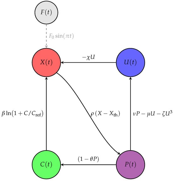
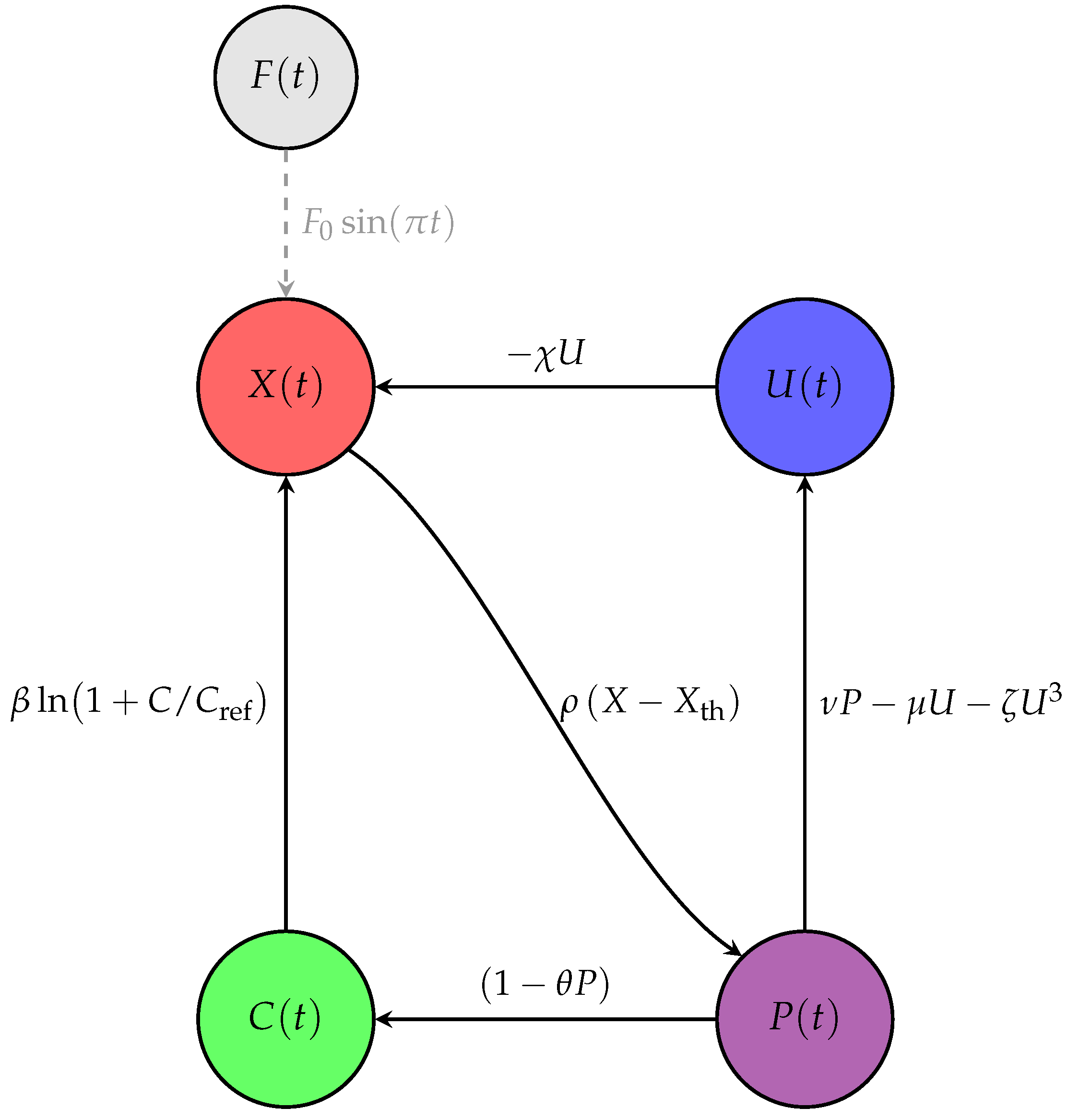
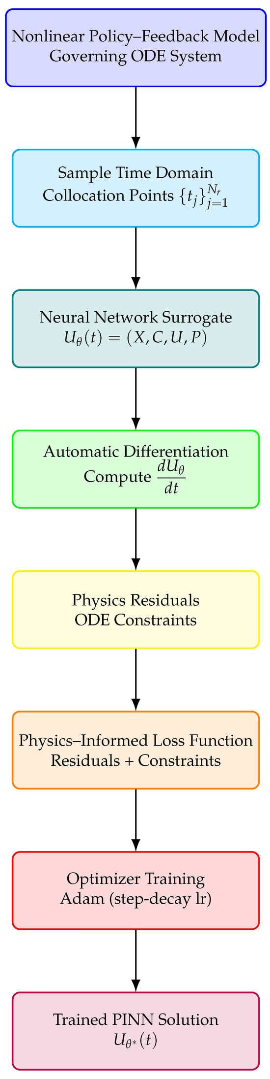
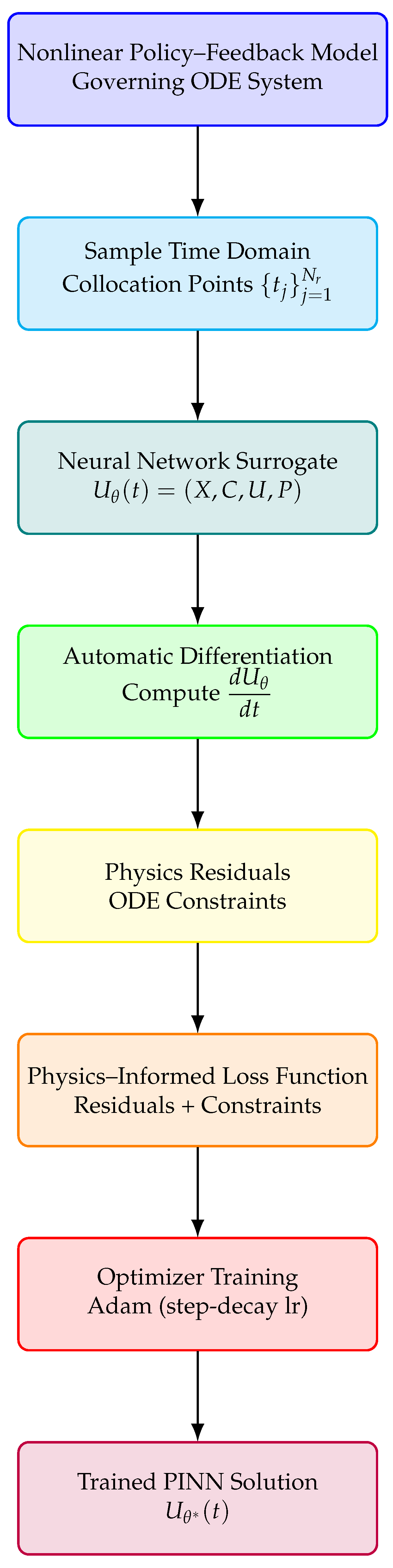
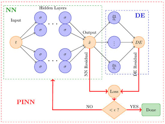
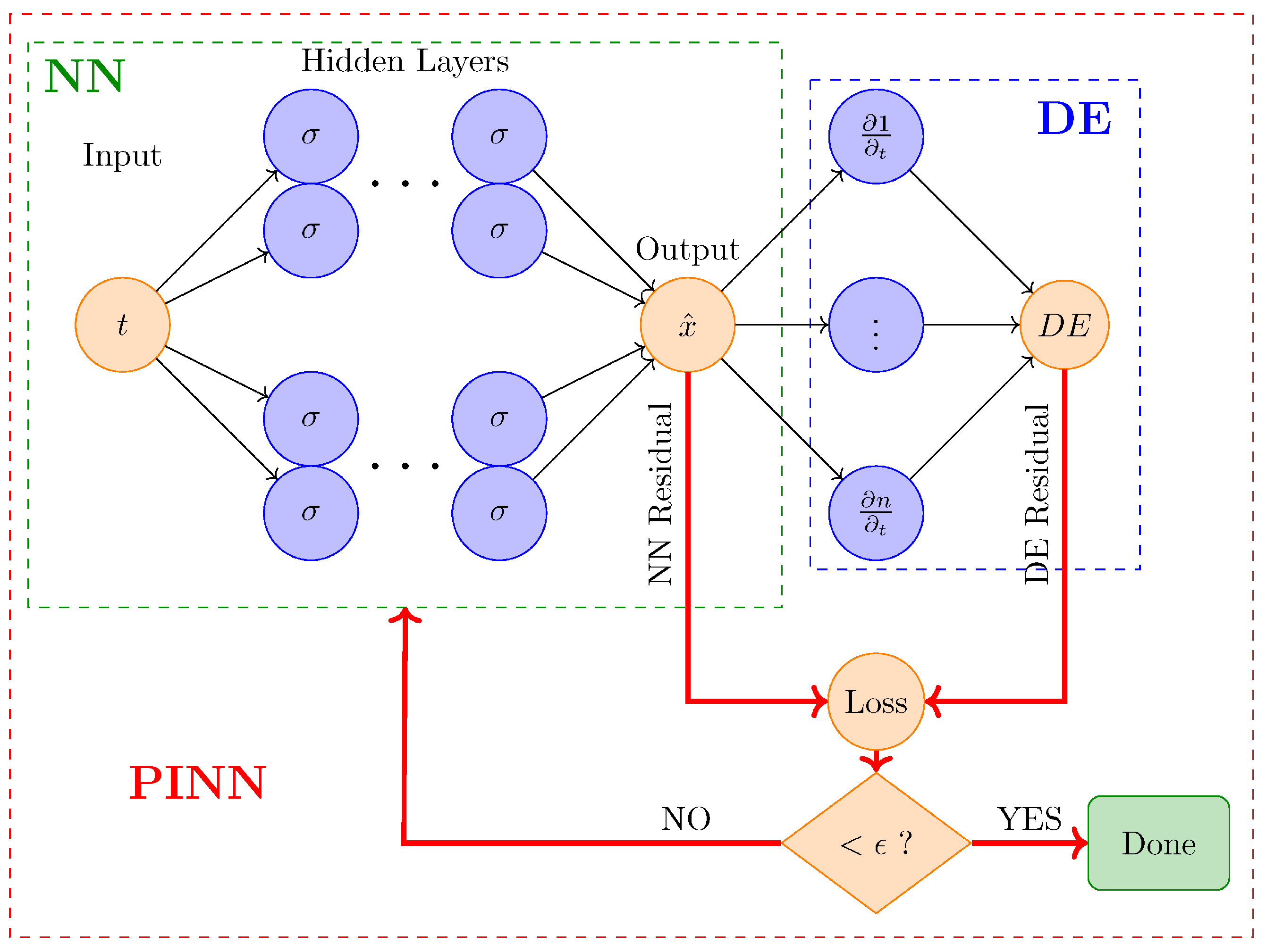
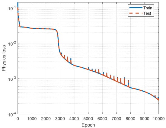
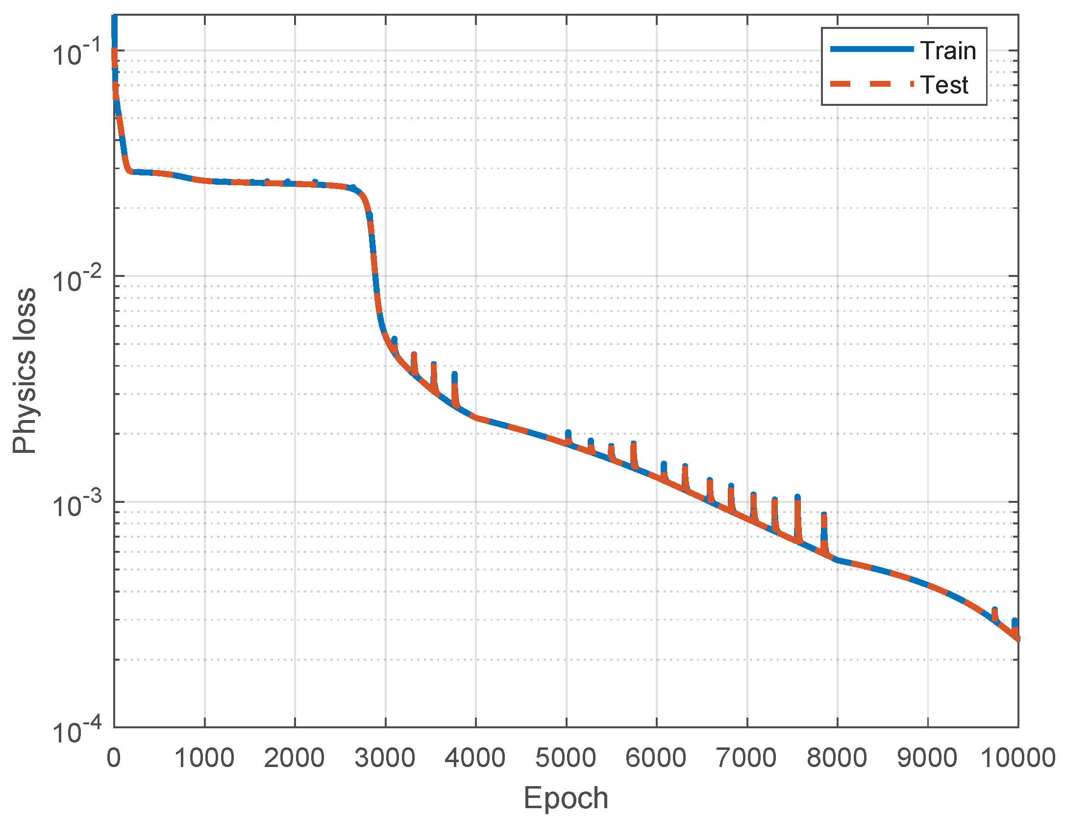
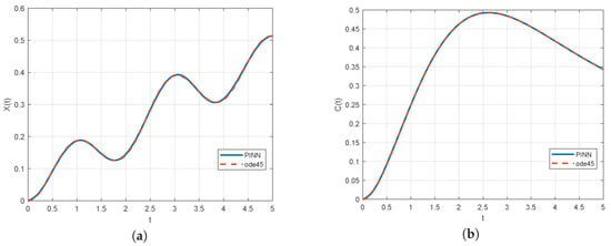
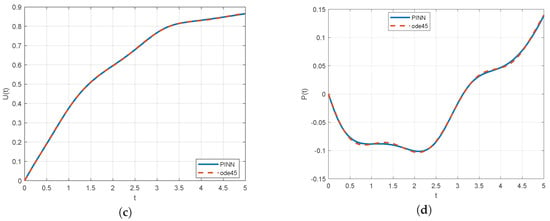
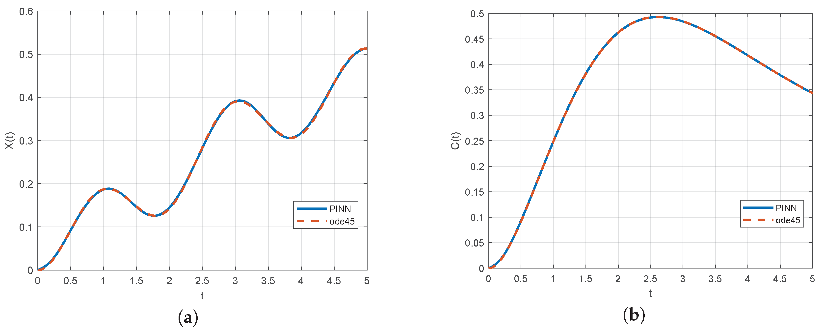
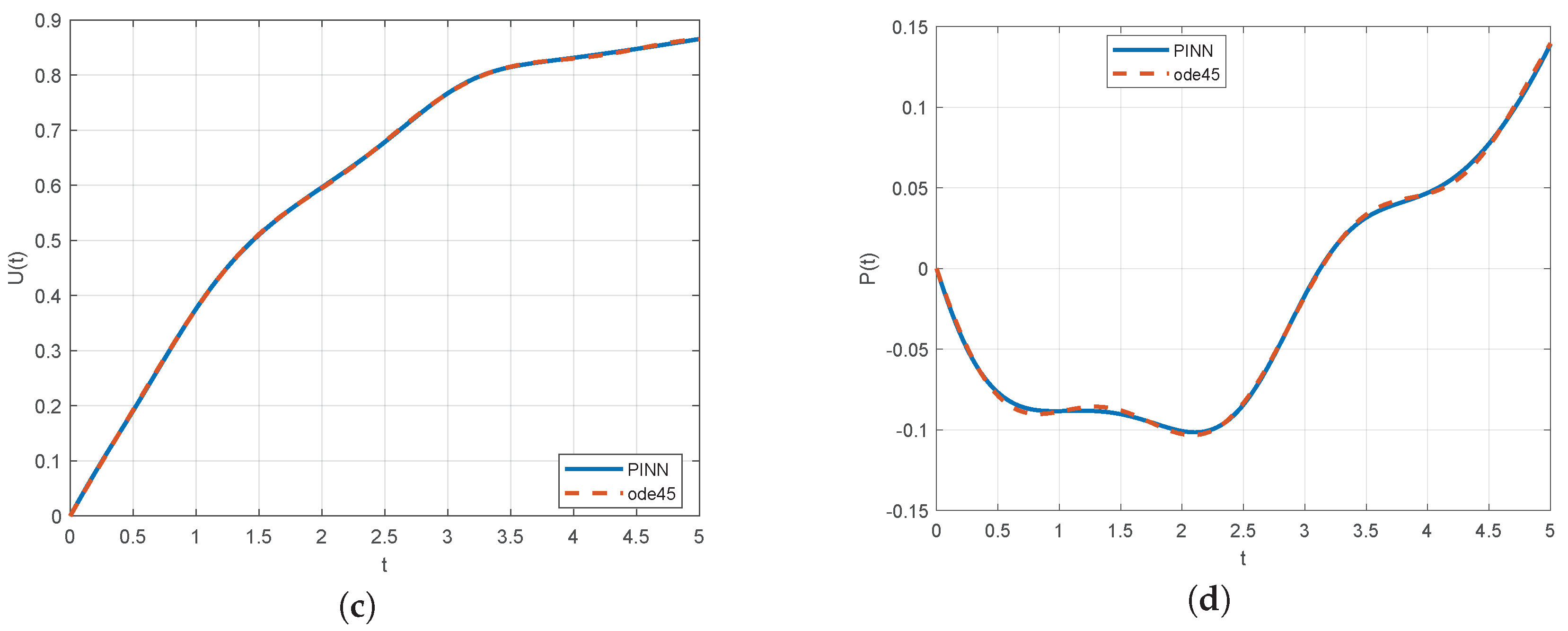
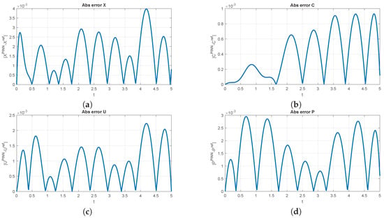
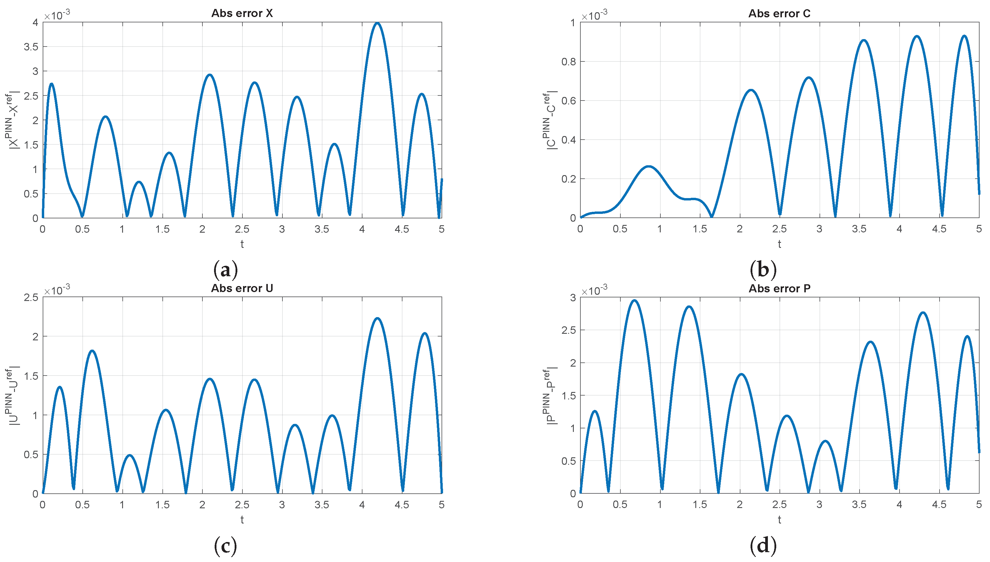
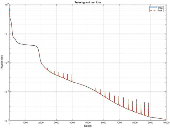
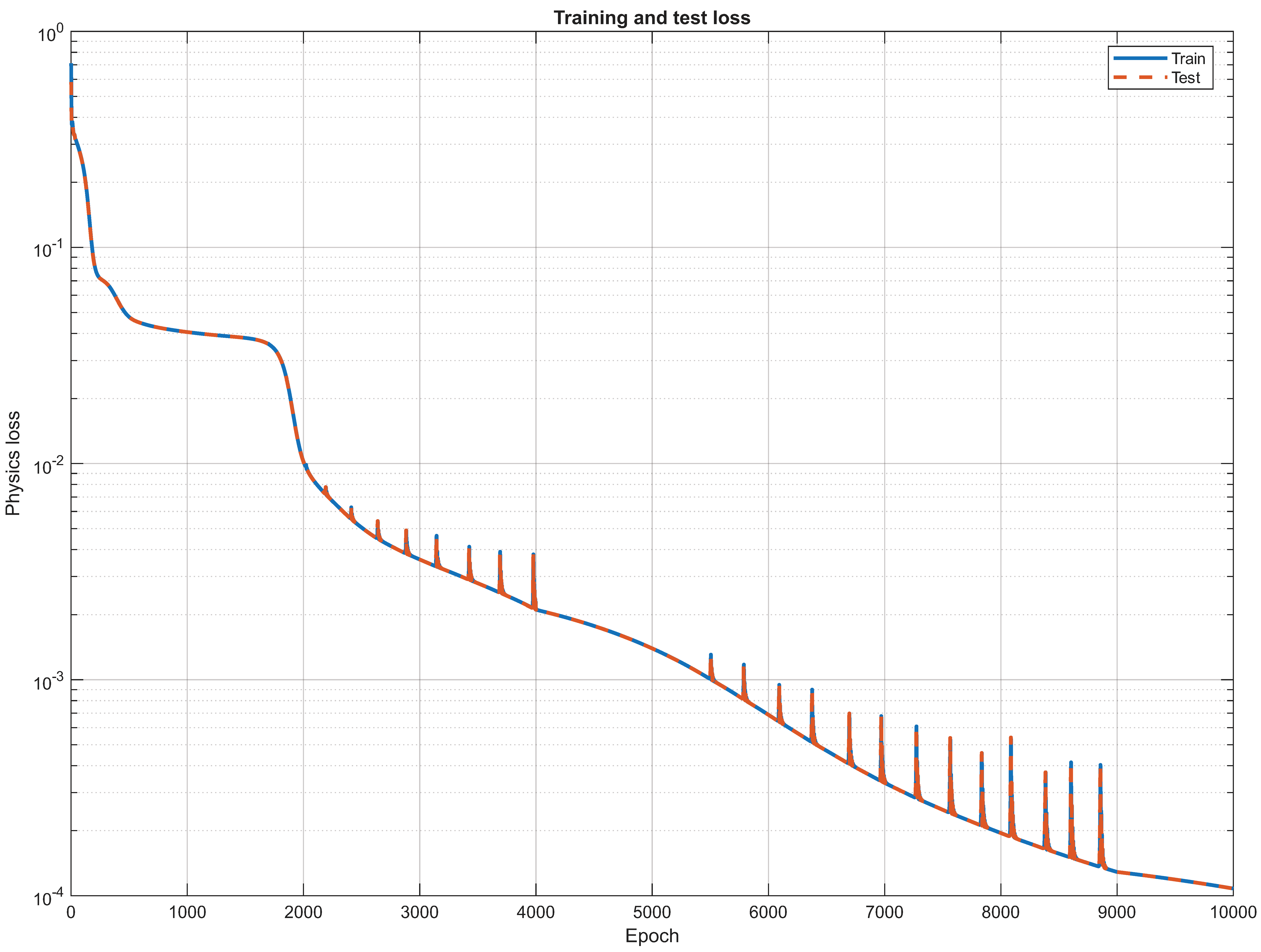
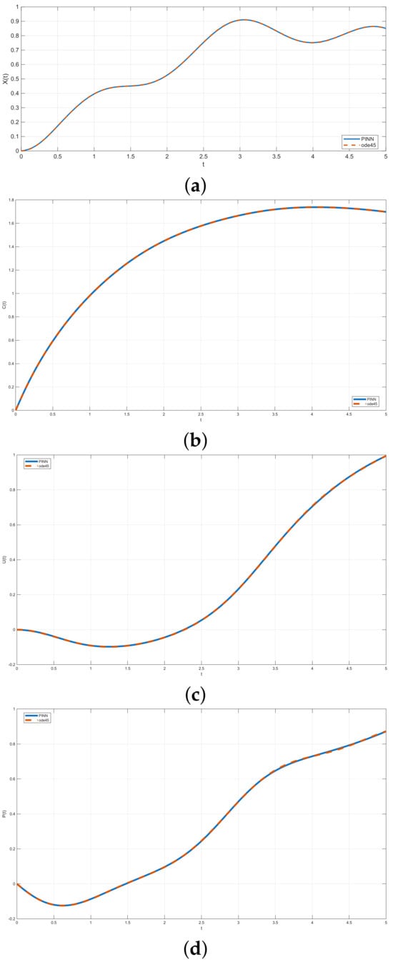
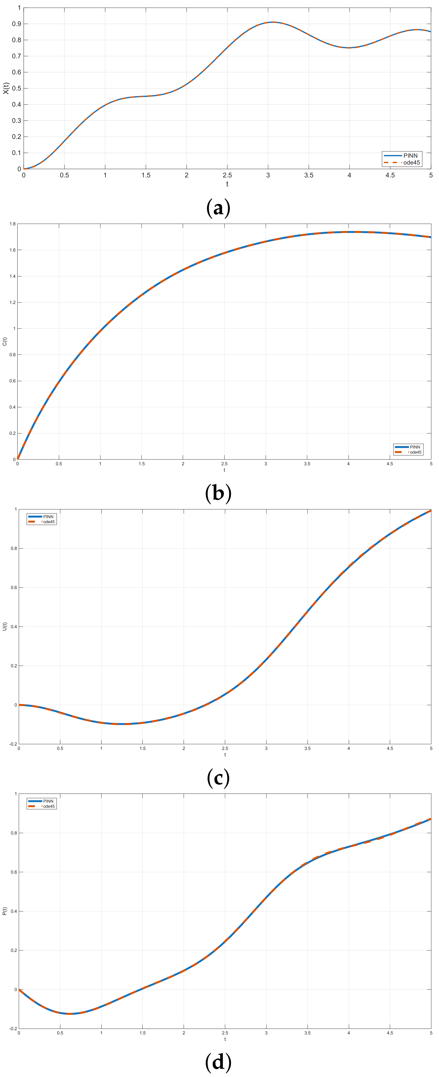
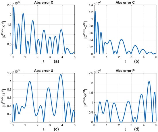
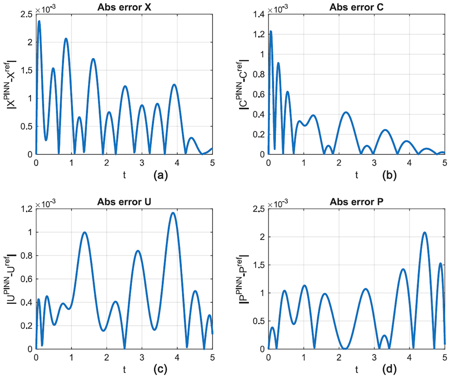

Disclaimer/Publisher’s Note: The statements, opinions and data contained in all publications are solely those of the individual author(s) and contributor(s) and not of MDPI and/or the editor(s). MDPI and/or the editor(s) disclaim responsibility for any injury to people or property resulting from any ideas, methods, instructions or products referred to in the content. |
© 2026 by the authors. Licensee MDPI, Basel, Switzerland. This article is an open access article distributed under the terms and conditions of the Creative Commons Attribution (CC BY) license.