Constraint-Adjusted Nonparametric Inference for Residual-Life Functionals Under Stochastic Precedence

Abstract

Nonparametric inference for residual-life functionals is a fundamental problem in mathematical statistics, reliability theory, and survival analysis, particularly in studies with limited sample sizes where empirical plug-in estimators may exhibit substantial sampling variability. In comparative lifetime analysis, additional qualitative information is often available regarding the relative behavior of two populations; however, such information is frequently too weak to justify classical stochastic dominance assumptions. Stochastic precedence provides a natural and interpretable framework for representing this partial ordering through a pairwise probabilistic constraint. This paper develops a constraint-adjusted nonparametric inference framework for estimating the mean residual life (MRL) and quantile residual life (QRL) functions under stochastic precedence information. The proposed approach replaces the ordinary empirical distribution function in standard residual-life plug-in estimators with a constraint-adjusted empirical distribution function that enforces the stochastic precedence relation at the sample level. The adjustment is governed by a data-driven scaling factor and is asymptotically negligible, thereby preserving the large-sample behavior of the ordinary empirical estimators while incorporating meaningful structural information in finite samples. Strong consistency of the proposed MRL and QRL estimators was established under mild regularity conditions. A Monte Carlo study based on Weibull and gamma lifetime models demonstrates that in the simulation settings considered, the proposed estimators provide improved finite-sample stability and generally achieve smaller mean squared errors than their ordinary empirical counterparts, especially for small and moderate sample sizes. The methodology is further illustrated using survival data from patients with squamous cell carcinoma of the oropharynx, highlighting its practical relevance in biomedical survival analysis. The proposed method offers a flexible, interpretable, and computationally simple framework for nonparametric inference with structured lifetime data under weak stochastic ordering information.

1. Introduction

Nonparametric inference for lifetime and survival data is a central topic in mathematical statistics, particularly when the objective is to estimate functionals that describe the future behavior of a unit or subject conditional on survival up to a given time. Among such functionals, residual-life measures play a fundamental role in reliability theory, survival analysis, maintenance planning, and biomedical studies. For a nonnegative lifetime random variable, residual-life functionals characterize the remaining lifetime beyond a specified time point and therefore provide information that is more dynamic and decision-oriented than unconditional distributional summaries. The mean residual life (MRL) and quantile residual life (QRL) functions are especially important because they describe complementary aspects of the conditional residual lifetime distribution. The MRL function measures the expected remaining lifetime, whereas the QRL function provides quantile-based information that is less dependent on moment assumptions and may be more informative for skewed or heavy-tailed lifetime distributions [1,2,3].

For a nonnegative lifetime random variable $X$ with distribution function $F$ and survival function $\bar{F}=1-F$, the MRL function is defined by:

$$e(x)=E(X-x\mid X>x)={\displaystyle \frac{1}{\bar{F}\left(x\right)}}{\int }_x^{\mathrm{\infty }} \bar{F}(u)du,\bar{F}(x)>0.$$

For $\alpha \in (0,1)$, with $\bar{\alpha }=1-\alpha$, the QRL function is defined by:

$$q_{\alpha }\left(x\right)=Q_{\alpha }\left(X-x∣X>x\right)={\bar{F}}^{-1}\left(\bar{\alpha }\bar{F}\left(x\right)\right)-x,$$

where $Q_{\alpha }(Z)$ denotes the $\alpha$-quantile of a random variable $Z$, and ${\bar{F}}^{-1}$ denotes the generalized inverse of $\bar{F}$, defined by:

$${\bar{F}}^{-1}\left(t\right)=\mathrm{i}\mathrm{n}\mathrm{f}\left\{u:\bar{F}\left(u\right)\le t\right\}.$$

These functionals are particularly useful because they provide conditional summaries of the remaining lifetime distribution and can therefore support decision-making in reliability assessment, replacement policies, medical prognosis, and risk evaluation.

Nonparametric estimation of residual-life functionals is commonly based on empirical plug-in procedures, in which the unknown distribution or survival function is replaced by its empirical counterpart. Such estimators are attractive because they are distribution-free, easy to implement, and do not require specifying a parametric lifetime model [4,5,6,7,8]. However, their finite-sample behavior may be sensitive to sampling variability, especially in tail regions where fewer observations remain beyond the conditioning time point. This difficulty is particularly relevant in reliability and survival studies, where sample sizes are often small or moderate and estimation at later time points may be affected by substantial uncertainty. Moreover, ordinary empirical plug-in estimators do not exploit additional structural information that may be available in comparative lifetime studies. In many applications, two systems, treatments, devices, or patient groups may be expected to exhibit a directional ordering in their lifetimes, although the available information may be too weak to justify a strong stochastic dominance assumption. Ignoring such information may lead to avoidable variability, whereas imposing an overly restrictive order may distort the analysis.

Stochastic precedence provides a natural and interpretable compromise between unrestricted empirical estimation and classical stochastic dominance [9,10]. For two independent lifetime random variables $X$ and $Y$, the relation $X{\le }_{sp}Y$ is defined by:

$$P\left(X\le Y\right)\ge {\displaystyle \frac{1}{2}}.$$

When $X$ and $Y$ have distribution functions $F$ and $G$, respectively, this relation is equivalently written as $F{\le }_{sp}G$. Thus, stochastic precedence requires only that a randomly selected lifetime from one population tends to be no larger than a randomly selected lifetime from the other population with probability at least one half. This condition is substantially weaker than the usual stochastic order because it does not require pointwise ordering of distribution functions or survival functions. At the same time, it is directly interpretable through pairwise comparisons and can be empirically assessed from two independent samples. These features make stochastic precedence especially attractive in applications where partial ordering information is scientifically plausible but classical stochastic ordering is too strong.

Although stochastic precedence has been investigated as a weak stochastic ordering concept [9,10] and has been used in constrained distributional estimation [8], its role in nonparametric inference for residual-life functionals remains largely unexplored. This gap is important because residual-life measures are not simple distributional summaries; rather, they are conditional functionals that depend on the survival behavior beyond a specified time point. Consequently, incorporating stochastic precedence into MRL and QRL estimation requires more than a direct modification of the empirical distribution function. It requires a coherent procedure that respects the weak ordering information, preserves the nonparametric nature of empirical plug-in estimation, and retains valid large-sample behavior. Developing such a procedure is the main motivation of the present work.

The novelty of this paper is to address this problem by developing a constraint-adjusted nonparametric inference framework for estimating the MRL and QRL functions under stochastic precedence information. For this purpose, we apply the distribution function estimator defined by Arcones et al. [8], which is the main foundation of our work. The proposed approach replaces the ordinary empirical distribution function in standard residual-life plug-in estimators with a constraint-adjusted empirical distribution function. The adjustment enforces the stochastic precedence relation at the sample level through a data-driven scaling factor. At the same time, this factor converges to unity under suitable regularity conditions, so that the resulting adjusted empirical estimator remains asymptotically equivalent to the ordinary empirical estimator. This construction allows weak ordering information to be incorporated in finite samples without imposing a parametric lifetime model or a strong stochastic dominance assumption. The methodological value of the proposed approach lies in its ability to bridge two common but opposing strategies in lifetime-data analysis. On the one hand, unrestricted empirical estimation is flexible but may be unstable in small samples or tail regions. On the other hand, strongly ordered or parametric models may be efficient but can be scientifically unjustified when the available information supports only a weak directional comparison.

The remainder of the paper is organized as follows. Section 2 introduces the stochastic precedence framework and the corresponding constraint-adjusted distribution estimator. Section 3 develops the proposed constraint-adjusted estimators of the MRL and QRL functions and establishes their strong consistency. Section 4 presents the Monte Carlo simulation study and compares the finite-sample performance of the proposed estimators with ordinary empirical plug-in estimators. Section 5 provides a real-data application to the survival times of patients with squamous cell carcinoma of the oropharynx. Section 6 concludes the paper and discusses possible extensions.

2. Constraint-Adjusted Distribution Estimation Under Stochastic Precedence

The proposed residual-life methodology is built on a distributional estimator that is able to incorporate weak stochastic ordering information without abandoning the nonparametric nature of empirical inference. In the absence of structural information, the empirical distribution function is the standard estimator of an unknown lifetime distribution. Its main appeal lies in its distribution-free construction, computational simplicity, and well-established asymptotic properties. However, in comparative lifetime studies, the ordinary empirical estimator may fail to reflect scientifically meaningful information about the relative behavior of two populations. This issue is particularly relevant in small and moderate samples, where random fluctuations may obscure weak ordering patterns even when such patterns are supported by prior knowledge or by the broader experimental setting.

Stochastic precedence provides a suitable framework for incorporating such information. Unlike the usual stochastic order, it does not require a pointwise ordering between distribution or survival functions. Instead, it imposes only a pairwise probabilistic comparison between two independent lifetime variables. This makes it sufficiently weak to be realistic in many applications, while still being strong enough to guide constrained estimation. The aim of this section is therefore to introduce a constraint-adjusted empirical distribution estimator that enforces stochastic precedence at the sample level and serves as the foundation for the residual-life estimators developed in the next section.

Assume first that $X{\le }_{sp}Y$, and that the distribution function $G$ of $Y$ is known. Let $X_1,X_2,\dots ,X_n$ be a random sample from the distribution function $F$ of $X$. Define

$$\varphi \left(x\right)=G\left(x-\right)-{\displaystyle \frac{1}{2}},$$

where $G(x-)$ denotes the left limit of $G$ at $x$. Since

$$X{\le }_{sp}Y⟺P(X\le Y)\ge {\displaystyle \frac{1}{2}},$$

the stochastic precedence condition can be expressed as

$$\int \varphi (x)dF(x)\le 0.$$

This representation is important because it converts stochastic precedence into a linear distributional constraint on $F$. Consequently, the weak ordering information can be incorporated into a nonparametric estimator without specifying a parametric lifetime model and without imposing a full stochastic dominance relation.

To enforce this constraint empirically, define the data-dependent scaling parameter

$${\widehat{a}}_n=\mathrm{s}\mathrm{u}\mathrm{p}\left\{a\ge 0:{\displaystyle \frac{1}{n}}{\displaystyle \sum _{i=1}^n} \varphi \left(a{X}_i\right)\le 0\right\}.$$

(1)

Let ${\lambda }_n=\mathrm{m}\mathrm{i}\mathrm{n}\left\{{\widehat{a}}_n,1\right\}$. The corresponding constraint-adjusted empirical estimator of $F$ is given by:

$$F_n^{\ast }(x)={\displaystyle \frac{1}{n}}{\displaystyle \sum _{i=1}^n} I\left({\lambda }_n{X}_i\le x\right).$$

(2)

Thus, $F_n^{\ast }$ is obtained by forming the empirical distribution function after rescaling the observed lifetimes by the factor ${\lambda }_n$. The role of this factor is not to impose a parametric transformation on the data, but to make the empirical distribution compatible with the stochastic precedence constraint. The truncation ${\lambda }_n\le 1$ ensures that the adjustment is made only in the direction required to restore this compatibility. The adjustment should not be interpreted as empirical validation of the stochastic precedence assumption. Rather, it constructs a constrained empirical estimator under a prespecified weak ordering direction. When the ordinary empirical distribution already satisfies the constraint, the adjustment is inactive, and the resulting estimator coincides with the usual empirical estimator. By construction,

$$\int \varphi (x)d{F}_n^{\ast }(x)\le 0,$$

and therefore

$$F_n^{\ast }{\le }_{sp}G.$$

This finite-sample property is the main reason for using $F_n^{\ast }$ instead of the ordinary empirical distribution function. It guarantees that the estimator respects the available stochastic precedence information, rather than allowing random sampling variation to violate it. At the same time, the procedure remains fully nonparametric: no parametric form is assumed for $F$, and no pointwise ordering between $F$ and $G$ is imposed. Moreover, the scaling adjustment is asymptotically negligible under standard regularity conditions, so that $F_n^{\ast }$ is asymptotically equivalent to the ordinary empirical distribution function $F_n$. Hence, the estimator combines finite-sample structural coherence with the large-sample validity of empirical inference.

In practical comparative studies, the distribution function $G$ is usually unknown and must be estimated from data. Let $X_1,\dots ,X_n$ and $Y_1,\dots ,Y_m$ be independent samples from $F$ and $G$, respectively. In this two-sample setting, the stochastic precedence information can be represented through the pairwise comparison functional:

$$H(t)=P(Y<tX).$$

The functional measures the extent to which a scaled version of $X$ is compatible with the precedence relation relative to $Y$. Its empirical counterpart is the $U$-type statistic:

$$H_{n,m}(t)={\displaystyle \frac{1}{nm}}{\displaystyle \sum _{i=1}^n} {\displaystyle \sum _{j=1}^m} I\left(Y_j<t{X}_i\right).$$

The corresponding two-sample scaling parameter is defined by:

$${\widehat{a}}_{n,m}=\mathrm{s}\mathrm{u}\mathrm{p}\left\{a\ge 0:H_{n,m}(a)\le {\displaystyle \frac{1}{2}}\right\}.$$

(3)

Set

$${\lambda }_{n,m}=\mathrm{m}\mathrm{i}\mathrm{n}\left\{{\widehat{a}}_{n,m},1\right\}.$$

Computationally, the scaling factor can be obtained by evaluating the relevant pairwise comparison thresholds and sorting the admissible values, rather than by using a dense grid search. Therefore, the procedure remains practical for the small and moderate sample sizes considered in this study. Note that the construction of the two-sample scaling factor is a direct generalization of the corresponding single-sample construction.

The two-sample constraint-adjusted empirical estimator of $F$ is then defined as:

$$F_{n,m}^{\ast }(x)={\displaystyle \frac{1}{n}}{\displaystyle \sum _{i=1}^n} I\left({\lambda }_{n,m}{X}_i\le x\right).$$

(4)

This estimator extends the known-$G$ construction by using pairwise comparisons between the two samples to determine the amount of adjustment required. The adjustment is therefore entirely data-driven and depends on the empirical evidence supplied by both samples. The scaling factor ${\lambda }_{n,m}$, which is smaller than 1, ensures that the transformed data satisfy the stochastic precedence constraint. If $G_m$ denotes the empirical distribution function based on $Y_1,\dots ,Y_m$, then $F_{n,m}^{\ast }{\le }_{sp}{G}_m,$ so that the stochastic precedence relation is enforced directly at the empirical level.

The estimator $F_{n,m}^{\ast }$ has three features that make it particularly suitable for the present problem. First, it preserves the distribution-free character of empirical estimation and is simple to compute. Second, it incorporates weak ordering information without requiring the stronger and often unrealistic assumption of usual stochastic ordering. Third, because the scaling factor converges to one under suitable conditions, the adjustment does not change the first-order asymptotic behavior of the empirical distribution estimator. These properties make $F_{n,m}^{\ast }$ an appropriate building block for nonparametric inference on conditional lifetime functionals.

The contribution of the present work begins at this point. The estimator $F_{n,m}^{\ast }$ provides a constraint-adjusted distributional input; however, residual-life inference requires transferring this adjustment from the distributional level to conditional lifetime functionals. This transfer is not merely a formal substitution, since the MRL function depends on an integrated-tail functional, whereas the QRL function depends on a generalized inverse of the survival function. Accordingly, the next section develops the corresponding constraint-adjusted plug-in estimators for the MRL and QRL functions and establishes that the stochastic precedence adjustment preserves strong consistency for both types of residual-life functionals. The resulting estimators inherit the nonparametric structure and large-sample validity of empirical plug-in methods while incorporating stochastic precedence information at the finite-sample level.

3. Constraint-Adjusted Estimation of the MRL and QRL Functions

The stochastic precedence relation $X{\le }_{sp}Y$ provides weak but meaningful structural information on the comparative behavior of two lifetime populations. The constraint-adjusted empirical distribution function $F_{n,m}^{\ast }$ introduced in Section 2 incorporates this information at the distributional level while retaining the nonparametric character of empirical inference. We now propagate this adjustment from the distribution function to residual-life functionals. The main principle is functional. The MRL and QRL functions are viewed as plug-in functionals of the underlying survival distribution. Instead of evaluating these functionals at the ordinary empirical distribution $F_n$, we evaluate them at the constraint-adjusted empirical distribution $F_{n,m}^{\ast }$. This produces residual-life estimators that are structurally coherent with the stochastic precedence constraint in finite samples and asymptotically equivalent to their ordinary empirical counterparts. Thus, the proposed method extends constraint-adjusted empirical estimation from the distributional level to conditional lifetime inference.

Throughout this section, ${\bar{F}}_{n,m}^{\ast }=1-F_{n,m}^{\ast }$ denotes the adjusted empirical survival function. We use the following standard regularity condition, which is inherited from the constraint-adjusted distributional estimator introduced in Section 2.

Assumption 1

(Consistency of the adjusted empirical distribution). As $n,m\to \mathrm{\infty }$, the adjusted empirical distribution satisfies

$$\underset{t\ge 0}{\mathrm{s}\mathrm{u}\mathrm{p}} \left|F_{n,m}^{\ast }(t)-F(t)\right|⟶0\mathrm{a}.\mathrm{s}.,$$

and the associated scaling factor satisfies  ${\lambda }_{n,m}⟶1a.s.$Consequently,

$$\underset{t\ge 0}{\mathrm{s}\mathrm{u}\mathrm{p}}\left|{\bar{F}}_{n,m}^{\ast }(t)-\bar{F}(t)\right|⟶0\mathrm{a}.\mathrm{s}.$$

Assumption 1 is stated explicitly to separate the distributional convergence requirement from the residual-life arguments developed below. It is satisfied under the regularity conditions for stochastic-precedence-constrained empirical estimation established in the constrained distributional framework on which Section 2 is based [8,11]. Thus, Assumption 1 provides the distributional convergence foundation needed to transfer the constraint-adjusted empirical estimator to the residual-life plug-in estimators developed below. In the present paper, this assumption serves as the bridge that permits the finite-sample stochastic precedence adjustment to be propagated from the empirical distribution function to integrated-tail and quantile-type residual-life functionals.

3.1. Constraint-Adjusted Estimation of the MRL Function

Let $X_1,\dots ,X_n$ be a random sample from $F$, and let $F_n$ and ${\bar{F}}_n=1-F_n$ denote the empirical distribution and survival functions, respectively. The classical nonparametric estimator of the MRL function is obtained by replacing $\bar{F}$ with ${\bar{F}}_n$ in the integrated-tail representation of $e(x)$ [12]. Hence,

$$e_n\left(x\right)={\displaystyle \frac{1}{{\bar{F}}_n\left(x\right)}}{\int }_x^{\mathrm{\infty }} {\bar{F}}_n\left(u\right)du={\displaystyle \frac{{\displaystyle {\sum }_{i=1}^n} \left(X_i-x\right)I\left(X_i>x\right)}{{\displaystyle {\sum }_{i=1}^n} I\left(X_i>x\right)}}I\left(x<X_{\left(n\right)}\right),$$

(5)

where $X_{(n)}=\mathrm{m}\mathrm{a}\mathrm{x}\left\{X_1,\dots ,X_n\right\}$. The factor $I\left(x<X_{(n)}\right)$ emphasizes that the empirical MRL estimator is meaningful only on the region where the empirical survival function is positive. This estimator is distribution-free and does not require a parametric lifetime model, but it does not incorporate comparative information that may be available from a second population.

Suppose now that $F{\le }_{sp}G$, and let $X_1,\dots ,X_n$ and $Y_1,\dots ,Y_m$ be independent samples from $F$ and $G$, respectively. The constraint-adjusted distribution estimator $F_{n,m}^{\ast }$ induces the adjusted survival function ${\bar{F}}_{n,m}^{\ast }$. We define the constraint-adjusted MRL estimator by applying the MRL functional to ${\bar{F}}_{n,m}^{\ast }$:

$$e_{n,m}^{\ast }\left(x\right)={\displaystyle \frac{1}{{\bar{F}}_{n,m}^{\ast }\left(x\right)}}{\int }_x^{\mathrm{\infty }} {\bar{F}}_{n,m}^{\ast }\left(u\right)du.$$

Using the explicit form of $F_{n,m}^{\ast }$, this estimator can be written as:

$$e_{n,m}^{\ast }(x)={\displaystyle \frac{{\displaystyle {\sum }_{i=1}^n} \left({\lambda }_{n,m}{X}_i-x\right)I\left({\lambda }_{n,m}{X}_i>x\right)}{{\displaystyle {\sum }_{i=1}^n} I\left({\lambda }_{n,m}{X}_i>x\right)}}I\left(x<{\lambda }_{n,m}{X}_{(n)}\right).$$

(6)

Thus, $e_{n,m}^{\ast }(x)$ is precisely the empirical MRL estimator computed from the adjusted sample ${\lambda }_{n,m}{X}_1,\dots ,{\lambda }_{n,m}{X}_n$. This representation clarifies the role of the adjustment. If the empirical samples already satisfy the stochastic precedence constraint, then ${\lambda }_{n,m}=1$, and $e_{n,m}^{\ast }(x)=e_n(x)$. Otherwise, the sample is minimally rescaled so that the resulting empirical distribution is compatible with the stochastic precedence information. Hence, the estimator remains nonparametric, but it is structurally informed by the weak ordering relation between the two populations.

The following theorem establishes that this finite-sample adjustment does not change the population MRL target.

Theorem 1.

Assume that  $E(X)<\infty$. Let  $x\ge 0$  be fixed, and suppose that  $\bar{F}(x)>0$. Under Assumption 1,

$$e_{n,m}^{\ast }(x)⟶e(x)\mathrm{a}.\mathrm{s}.\mathrm{as}n,m\to \mathrm{\infty }.$$

Proof. 

By Assumption 1,

$${\bar{F}}_{n,m}^{\ast }(x)⟶\bar{F}(x)\mathrm{a}.\mathrm{s}.$$

Since $\bar{F}(x)>0$, the denominator of $e_{n,m}^{\ast }(x)$ is eventually positive almost surely. Note that as the sample sizes increase, the scaling factor converges to 1. It remains to establish the convergence of the integrated-tail term. From the explicit adjusted sample representation,

$${\int }_x^{\mathrm{\infty }} {\bar{F}}_{n,m}^{\ast }(u)du={\displaystyle \frac{1}{n}}{\displaystyle {\sum }_{i=1}^n} {\left({\lambda }_{n,m}{X}_i-x\right)}_{+},$$

where $(z{)}_{+}=\mathrm{m}\mathrm{a}\mathrm{x}\{z,0\}$. Since ${\lambda }_{n,m}\to 1$ almost surely, we have

$$\left|{\displaystyle \frac{1}{n}}{\displaystyle \sum _{i=1}^n} {\left({\lambda }_{n,m}{X}_i-x\right)}_{+}-{\displaystyle \frac{1}{n}}{\displaystyle \sum _{i=1}^n} {\left(X_i-x\right)}_{+}\right|\le \left|{\lambda }_{n,m}-1\right|{\displaystyle \frac{1}{n}}{\displaystyle \sum _{i=1}^n} X_i.$$

By the strong law of large numbers, $n^{-1}{\displaystyle {\sum }_{i=1}^n} X_i\to E(X)$ almost surely. Therefore, the right-hand side converges to zero almost surely. Again, by the strong law of large numbers,

$${\displaystyle \frac{1}{n}}{\displaystyle \sum _{i=1}^n} {\left(X_i-x\right)}_{+}⟶E\left[(X-x{)}_{+}\right] \mathrm{a}.\mathrm{s}.,$$

and, since $E(X)<\mathrm{\infty }$,

$$E\left[(X-x{)}_{+}\right]={\int }_x^{\mathrm{\infty }} \bar{F}\left(u\right)du.$$

Consequently,

$${\int }_x^{\mathrm{\infty }} {\bar{F}}_{n,m}^{\ast }(u)du⟶{\int }_x^{\mathrm{\infty }} \bar{F}(u)du\mathrm{a}.\mathrm{s}.$$

Combining the convergence of the numerator and denominator gives

$$e_{n,m}^{\ast }(x)={\displaystyle \frac{{\int }_x^{\mathrm{\infty }} {\bar{F}}_{n,m}^{\ast }(u)du}{{\bar{F}}_{n,m}^{\ast }(x)}}⟶{\displaystyle \frac{{\int }_x^{\mathrm{\infty }} \bar{F}(u)du}{\bar{F}(x)}}=e(x)\mathrm{a}.\mathrm{s}.$$

□

Theorem 1 shows that the proposed estimator is a consistent estimator of the same population MRL function targeted by the ordinary empirical estimator. Thus, the stochastic precedence adjustment acts as a finite-sample structural correction rather than a change in the estimand. This distinction is important: the method introduces additional information at the empirical level while preserving the underlying nonparametric target.

3.2. Constraint-Adjusted Estimation of the QRL Function

We next consider the QRL function. In contrast to the MRL function, the QRL function summarizes conditional residual lifetime through quantiles and therefore does not require moment assumptions. This makes it particularly useful in lifetime models with skewness, heavy tails, or heterogeneous residual behavior. For a random sample $X_1,\dots ,X_n$ from $F$, the standard empirical plug-in estimator of $q_{\alpha }\left(x\right),0<\alpha <1$, is

$$q_{\alpha ,n}(x)={\bar{F}}_n^{-1}\left\{\bar{\alpha }{\bar{F}}_n(x)\right\}-x,$$

(7)

where $\bar{\alpha }=1-\alpha$, and

$${\bar{F}}_n^{-1}(t)=\mathrm{i}\mathrm{n}\mathrm{f}\left\{u:{\bar{F}}_n(u)\le t\right\}$$

is the generalized inverse of the empirical survival function. This estimator is obtained by applying the QRL functional directly to the empirical survival distribution.

Under the stochastic precedence constraint $F{\le }_{sp}G$, we define the constraint-adjusted QRL estimator by applying the same functional to the adjusted survival estimator ${\bar{F}}_{n,m}^{\ast }$. Thus,

$$q_{\alpha ,n,m}^{\ast }\left(x\right)={\left({\bar{F}}_{n,m}^{\ast }\right)}^{-1}\left\{\bar{\alpha }{\bar{F}}_{n,m}^{\ast }\left(x\right)\right\}-x,$$

(8)

where

$${\left({\bar{F}}_{n,m}^{\ast }\right)}^{-1}\left(t\right)=\mathrm{i}\mathrm{n}\mathrm{f}\left\{u:{\bar{F}}_{n,m}^{\ast }\left(u\right)\le t\right\}.$$

Since the adjusted empirical survival function is a step function, its generalized inverse may have discontinuities at the jump points. Therefore, the proposed QRL estimator is interpreted through the usual generalized inverse, and the consistency result is stated at continuity points of the limiting quantile functional. This estimator is the QRL analogue of $e_{n,m}^{\ast }(x)$. It reduces to $q_{\alpha ,n}(x)$ whenever the empirical constraint is inactive, and otherwise evaluates the quantile residual-life functional after enforcing stochastic precedence at the distributional level. Thus, the MRL and QRL estimators are generated by the same principle: replace the unconstrained empirical distribution by a constraint-adjusted empirical distribution before applying the desired residual-life functional.

The next theorem gives the strong consistency of the proposed QRL estimator.

Theorem 2.

Let  $x\ge 0$  be fixed, let  $0<\alpha <1$, and suppose that  $\bar{F}(x)>0$. Assume that  ${\bar{F}}^{-1}$ is continuous at  $t_x=\bar{\alpha }\bar{F}\left(x\right).$Under Assumption 1,

$$q_{\alpha ,n,m}^{*}(x)⟶q_{\alpha }(x)a.s.\mathrm{as}n,m\to \infty .$$

Proof. 

Under Assumption 1,

$$\underset{t\ge 0}{\mathrm{s}\mathrm{u}\mathrm{p}} \left|{\bar{F}}_{n,m}^{\ast }(t)-\bar{F}(t)\right|⟶0\mathrm{a}.\mathrm{s}.$$

Hence,

$${\bar{F}}_{n,m}^{\ast }(x)⟶\bar{F}(x)\mathrm{a}.\mathrm{s}.,$$

and consequently,

$$\bar{\alpha }{\bar{F}}_{n,m}^{\ast }(x)⟶\bar{\alpha }\bar{F}(x)=t_x\mathrm{a}.\mathrm{s}.$$

Uniform convergence of the adjusted survival functions implies convergence of the corresponding generalized inverse at continuity points of the limiting inverse map. Refer to Csorgo and Csorgo [13] for more information about the convergence of the generalized inverse function. Since ${\bar{F}}^{-1}$ is continuous at $t_x$, it follows that

$${\left({\bar{F}}_{n,m}^{\ast }\right)}^{-1}\left\{\bar{\alpha }{\bar{F}}_{n,m}^{\ast }(x)\right\}⟶{\bar{F}}^{-1}\{\bar{\alpha }\bar{F}(x)\}\mathrm{a}.\mathrm{s}.$$

Therefore,

$$q_{\alpha ,n,m}^{\ast }(x)⟶{\bar{F}}^{-1}\{\bar{\alpha }\bar{F}(x)\}-x=q_{\alpha }(x)\mathrm{a}.\mathrm{s}.$$

□

Remark  1.

The continuity condition imposed on  ${\bar{F}}^{-1}$ is the standard identifiability condition for quantile-type functionals. It rules out non-unique target quantiles caused by flat portions or discontinuities of the survival function at the level $t_x=\bar{\alpha }\bar{F}(x)$. Under this condition, uniform convergence of the adjusted survival estimator is transferred to the $QRL$ functional through the generalized inverse map [13].

Remark 2.

Theorems 1 and 2 show that the stochastic precedence adjustment is asymptotically neutral but finite-sample informative. Both  $e_{n,m}^{\ast }(x)$ and  $q_{\alpha ,n,m}^{\ast }(x)$ estimate the same population functionals as the ordinary empirical estimators. The contribution of the proposed method is not to redefine the MRL or QRL targets, but to evaluate them through an empirical distribution that respects weak stochastic ordering information. This provides a principled compromise between unrestricted nonparametric estimation and strongly constrained stochastic-order models.

Remark 3.

The construction is functional in nature. Once a constraint-adjusted empirical distribution is available, any residual-life functional that is continuous with respect to the appropriate mode of convergence can, in principle, be estimated by the same plug-in mechanism. The MRL and QRL cases considered here are therefore representative of a broader class of conditional lifetime functionals for which weak ordering information may be incorporated without imposing a parametric model.

4. Monte Carlo Assessment of Finite-Sample Performance

This section presents a Monte Carlo study designed to evaluate the finite-sample performance of the proposed constraint-adjusted estimators. The objective is twofold. First, we examine whether the numerical behavior of the proposed estimators is consistent with the strong consistency results established in Section 3. Second, we assess whether incorporating stochastic precedence information into the empirical distribution can improve finite-sample estimation of residual-life functionals relative to ordinary empirical plug-in estimation.

The simulation focuses on two residual-life functionals: the MRL function and the median residual-life function, corresponding to the 0.5-quantile residual life. These two quantities are considered because they represent complementary features of the conditional residual lifetime distribution. The MRL function provides a moment-based summary of the expected remaining lifetime, whereas the median residual life provides a quantile-based summary that is less sensitive to tail behavior and does not rely on moment assumptions. Studying both functionals allows us to evaluate whether the proposed adjustment is effective for different types of residual-life summaries.

4.1. Simulation Design

Two flexible lifetime models are considered: the Weibull and gamma distributions. These models are widely used in reliability theory and survival analysis because they can represent different aging patterns, skewness levels, and tail behaviors. For the Weibull distribution, the survival function is given by:

$$\bar{F}(t)=\mathrm{e}\mathrm{x}\mathrm{p}\left\{-(\theta t{)}^k\right\},t\ge 0,$$

where $k>0$ is the shape parameter and $\theta >0$ is a scale-related parameter. For the gamma distribution, the survival function is written as:

$$\bar{F}(t)=1-{\displaystyle \frac{\mathsf{\gamma }\left(a,bt\right)}{\Gamma \left(a\right)}},t\ge 0,$$

where $a>0$ and $b>0$ are the shape and rate parameters, respectively, $\mathsf{\gamma }(a,bt)$ denotes the lower incomplete gamma function, and $\Gamma (a)$ denotes the complete gamma function.

For each lifetime model, parameter configurations are selected for the two random variables $X$ and $Y,$ so that the stochastic precedence relation $F{\le }_{sp}G$ is satisfied. In the reported parameter pairs, the subscript-2 parameter set is assigned to $X$ and the subscript-1 parameter set to $Y$. Independent samples are generated from $F$ and $G$ with equal sample sizes $n=m=25,50,100.$ These sample sizes represent small, moderate, and relatively larger sample settings, which are typical in reliability and biomedical survival applications. For each configuration, the number of Monte Carlo replications is fixed at $R=1000$.

In each replication, the empirical precedence rate is computed, and the scaling factor ${\lambda }_{n,m}$ is obtained according to the constraint-adjusted procedure described in Section 2. The proposed constraint-adjusted estimators and their ordinary empirical counterparts are then evaluated at three residual-life points $q_1,q_2$, and $q_3$, corresponding respectively to the first, second, and third quartiles of the distribution of $X$. This choice allows the estimators to be assessed across early, central, and later regions of the lifetime distribution.

4.2. Performance Measures

The finite-sample performance is evaluated using empirical bias and mean squared error (MSE). For a generic estimator $\widehat{\eta }(x)$ of a residual-life functional $\eta (x)$, the empirical bias is defined by:

$$\mathrm{B}\mathrm{i}\mathrm{a}\mathrm{s}\{\widehat{\eta }(x)\}={\displaystyle \frac{1}{R}}{\displaystyle \sum _{r=1}^R} \left\{{\widehat{\eta }}^{(r)}(x)-\eta (x)\right\},$$

and the empirical MSE is defined by:

$$\mathrm{M}\mathrm{S}\mathrm{E}\{\widehat{\eta }(x)\}={\displaystyle \frac{1}{R}}{\displaystyle \sum _{r=1}^R} {\left\{{\widehat{\eta }}^{(r)}(x)-\eta (x)\right\}}^2,$$

where ${\widehat{\eta }}^{(r)}(x)$ denotes the estimate obtained in the $r$-th Monte Carlo replication. The true values of the MRL and median residual-life functions are computed numerically from

$$e\left(x\right)={\displaystyle \frac{1}{\bar{F}\left(x\right)}}{\int }_x^{\mathrm{\infty }} \bar{F}\left(u\right)du,$$

and

$$q_{\alpha }\left(x\right)={\bar{F}}^{-1}\left\{\bar{\alpha }\bar{F}\left(x\right)\right\}-x,$$

with $\alpha =0.5$ for the median residual life.

4.3. Numerical Results

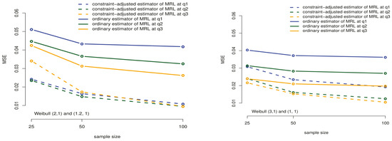
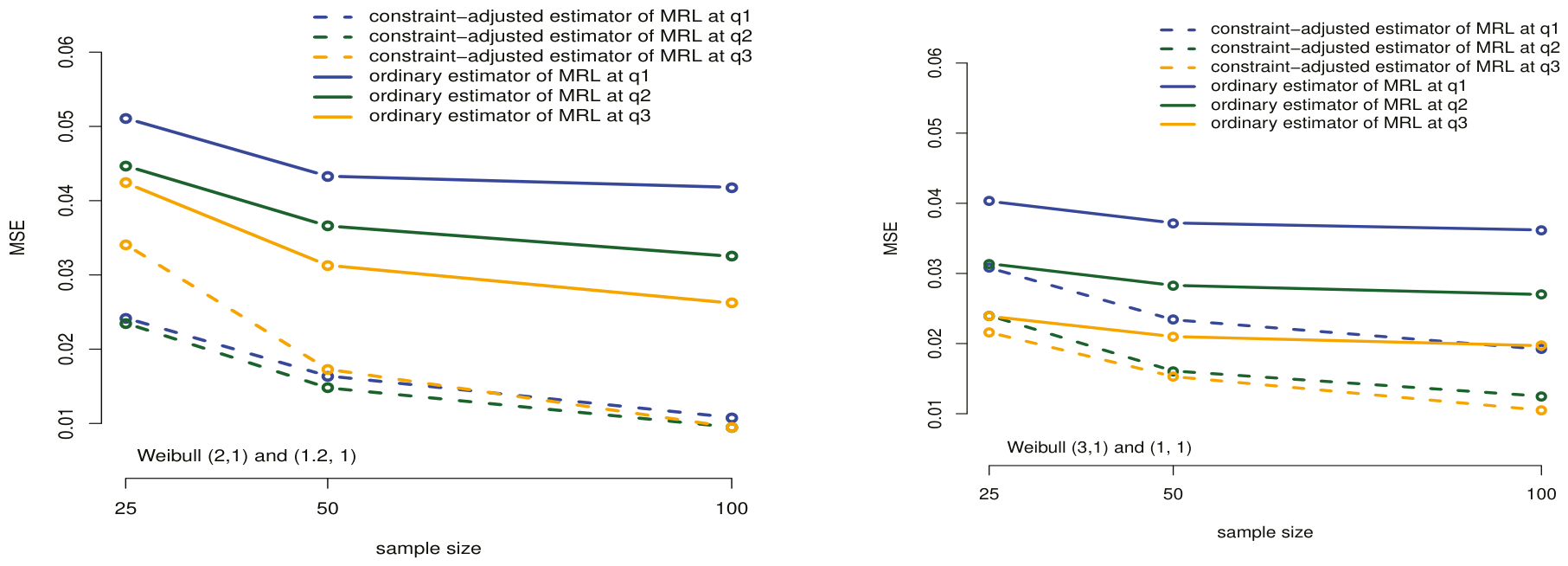
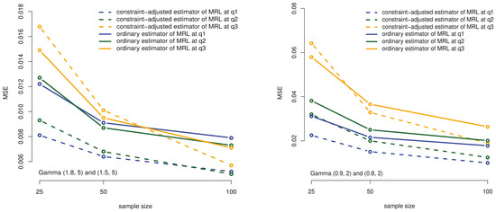
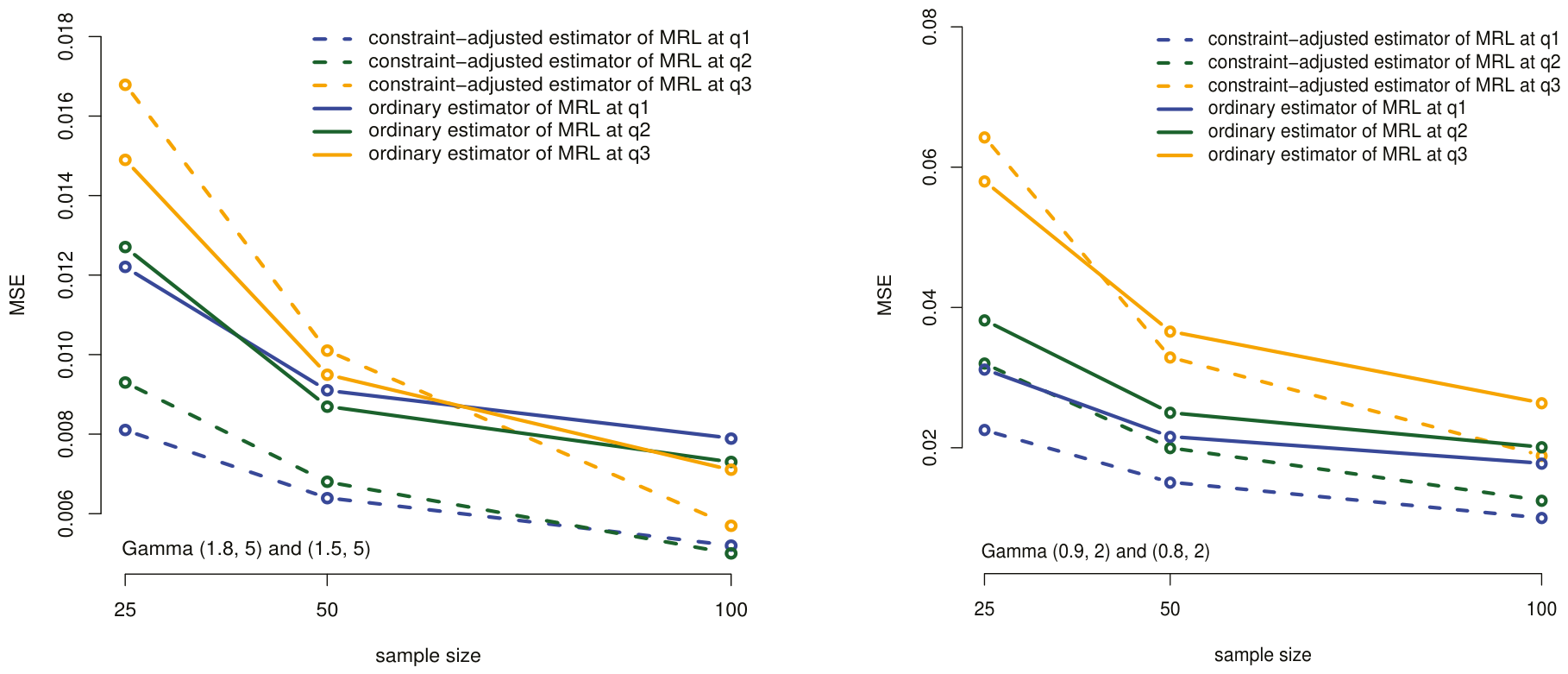
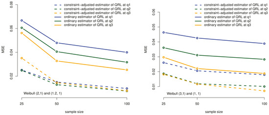
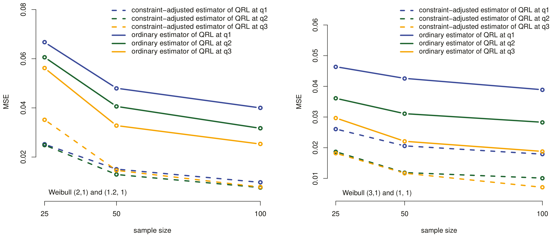
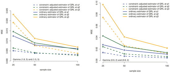
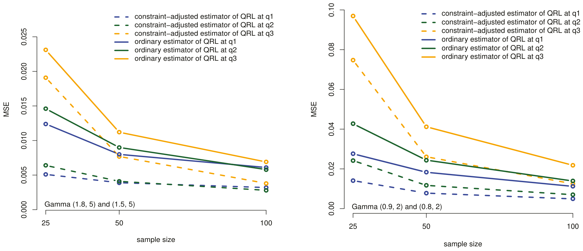
Table 1, Table 2, Table 3 and Table 4 report the Monte Carlo results. In each cell, the upper entry gives the empirical bias and the lower entry gives the corresponding MSE. Table 1 and Table 2 present the results for the MRL estimator under the Weibull and gamma lifetime models, respectively. Table 3 and Table 4 present the corresponding results for the median residual-life estimator. Figure 1, Figure 2, Figure 3 and Figure 4 also show a graphical investigation of the MSE values.

Table 1. Monte Carlo bias and mean squared error of the constraint-adjusted and ordinary empirical MRL estimators under the Weibull lifetime model. In each cell, the upper entry reports the bias and the lower entry reports the MSE.

n = m
Estimator	Parameters	$\mathit{q}$	25	50	100
Constraint-adjusted	$k_1=2$,${\theta }_1=1$, $k_2=1.2,{\theta }_2=1$	$q_1$	−0.0608	−0.0661	−0.0684
			0.0242	0.0164	0.0108
		$q_2$	−0.0494	−0.0541	−0.0604
			0.0235	0.0148	0.0095
		$q_3$	−0.0538	−0.0468	−0.0528
			0.0341	0.0173	0.0095
	$k_1=3$,${\theta }_1=1$, $k_2=1{,\theta }_2=1$	$q_1$	−0.1078	−0.117	−0.1216
			0.0308	0.0234	0.0192
		$q_2$	−0.0918	−0.0931	−0.0963
			0.024	0.0161	0.0125
		$q_3$	−0.0837	−0.0854	−0.0796
			0.0216	0.0153	0.0105
Ordinary	$k_1=2$,${\theta }_1=1$, $k_2=1.2{,\theta }_2=1$	$q_1$	0.1959	0.1921	0.1968
			0.0511	0.0433	0.0418
		$q_2$	0.1758	0.1727	0.1715
			0.0447	0.0366	0.0325
		$q_3$	0.1544	0.1516	0.1501
			0.0424	0.0313	0.0262
	$k_1=3$,${\theta }_1=1$, $k_2=1,{\theta }_2=1$	$q_1$	0.1865	0.1861	0.1869
			0.0403	0.0372	0.0362
		$q_2$	0.1621	0.161	0.1607
			0.0314	0.0283	0.027
		$q_3$	0.1357	0.1357	0.1356
			0.0239	0.021	0.0197

Table 2. Monte Carlo bias and mean squared error of the constraint-adjusted and ordinary empirical MRL estimators under the gamma lifetime model. In each cell, the upper entry reports the bias and the lower entry reports the MSE.

n = m
Estimator	Parameters	$\mathit{q}$	25	50	100
Constraint-adjusted	$a_1=1.8$,$b_1=5$, $a_2=1.5,b_2=5$	$q_1$	−0.0602	−0.0651	−0.0641
			0.0081	0.0064	0.0052
		$q_2$	−0.0549	−0.0603	−0.0586
			0.0093	0.0068	0.005
		$q_3$	−0.0569	−0.0547	−0.0525
			0.0168	0.0101	0.0057
	$a_1=0.9$,$b_1=2$, $a_2=0.8,b_2=2$	$q_1$	−0.0805	−0.072	−0.0717
			0.0225	0.0151	0.01
		$q_2$	−0.0807	−0.0762	−0.0718
			0.032	0.02	0.0125
		$q_3$	−0.0938	−0.0691	−0.071
			0.0643	0.0329	0.0189
Ordinary	$a_1=1.8$,$b_1=5$, $a_2=1.5,b_2=5$	$q_1$	0.084	0.0806	0.0809
			0.0122	0.0091	0.0079
		$q_2$	0.0799	0.0745	0.075
			0.0127	0.0087	0.0073
		$q_3$	0.0713	0.0678	0.0681
			0.0149	0.0095	0.0071
	$a_1=0.9$,$b_1=2$, $a_2=0.8,b_2=2$	$q_1$	0.1105	0.1137	0.1133
			0.0312	0.0216	0.0178
		$q_2$	0.1105	0.1121	0.1155
			0.0382	0.025	0.0201
		$q_3$	0.1056	0.1145	0.1187
			0.058	0.0366	0.0264

Table 3. Monte Carlo bias and mean squared error of the constraint-adjusted and ordinary empirical median residual-life estimators under the Weibull lifetime model. In each cell, the upper entry reports the bias and the lower entry reports the MSE.

n = m
Estimator	Parameters	$\mathit{q}$	25	50	100
Constraint-adjusted	$k_1=2$,${\theta }_1=1$, $k_2=1.2{,\theta }_2=1$	$q_1$	−0.0347	−0.0491	−0.0569
			0.0252	0.0151	0.0097
		$q_2$	−0.0099	−0.0338	−0.0435
			0.0249	0.0129	0.0076
		$q_3$	0.0076	−0.007	−0.0222
			0.0352	0.0146	0.0078
	$k_1=3$,${\theta }_1=1$, $k_2=1,{\theta }_2=1$	$q_1$	−0.0963	−0.1017	−0.113
			0.0261	0.0206	0.0179
		$q_2$	−0.0639	−0.0682	−0.0826
			0.0187	0.0119	0.0101
		$q_3$	−0.043	−0.0475	−0.0523
			0.0182	0.0117	0.0071
Ordinary	$k_1=2$,${\theta }_1=1$, $k_2=1.2,{\theta }_2=1$	$q_1$	0.2091	0.1946	0.1862
			0.0667	0.048	0.04
		$q_2$	0.1926	0.1726	0.1624
			0.0606	0.0406	0.0317
		$q_3$	0.1714	0.1409	0.1381
			0.0562	0.0328	0.0253
	$k_1=3$,${\theta }_1=1$, $k_2=1{,\theta }_2=1$	$q_1$	0.191	0.1924	0.1908
			0.0464	0.0426	0.0389
		$q_2$	0.1637	0.1622	0.1614
			0.0361	0.0311	0.0283
		$q_3$	0.1403	0.131	0.1283
			0.0297	0.0221	0.0188

Table 4. Monte Carlo bias and mean squared error of the constraint-adjusted and ordinary empirical median residual-life estimators under the gamma lifetime model. In each cell, the upper entry reports the bias and the lower entry reports the MSE.

n = m
Estimator	Parameters	$\mathit{q}$	25	50	100
Constraint-adjusted	$a_1=1.8$,$b_1=5$, $a_2=1.5,b_2=5$	$q_1$	−0.0393	−0.0438	−0.047
			0.0051	0.0039	0.0032
		$q_2$	−0.0222	−0.0325	−0.0383
			0.0064	0.0041	0.0028
		$q_3$	0.016	−0.0107	−0.0277
			0.0191	0.0077	0.0038
	$a_1=0.9$,$b_1=2$, $a_2=0.8,b_2=2$	$q_1$	−0.0353	−0.0404	−0.0434
			0.0141	0.0078	0.0049
		$q_2$	−0.018	−0.0301	−0.0405
			0.0242	0.0117	0.007
		$q_3$	0.0424	−0.0023	−0.0306
			0.0747	0.0261	0.0125
Ordinary	$a_1=1.8$,$b_1=5$, $a_2=1.5,b_2=5$	$q_1$	0.0773	0.0715	0.0676
			0.0124	0.008	0.0061
		$q_2$	0.0773	0.0695	0.0636
			0.0146	0.009	0.0058
		$q_3$	0.0924	0.0704	0.0625
			0.0231	0.0112	0.0069
	$a_1=0.9$,$b_1=2$, $a_2=0.8,b_2=2$	$q_1$	0.1022	0.0919	0.0844
			0.0276	0.0183	0.0112
		$q_2$	0.12	0.099	0.0876
			0.0427	0.0244	0.0139
		$q_3$	0.1726	0.1279	0.0952
			0.0969	0.0412	0.0218

Figure 1. Graphical comparison of the MSE values reported in Table 1 for the constraint-adjusted and ordinary empirical MRL estimators under the Weibull lifetime model across different sample sizes.

Figure 2. Graphical comparison of the MSE values reported in Table 2 for the constraint-adjusted and ordinary empirical MRL estimators under the gamma lifetime model across different sample sizes.

Figure 3. Graphical comparison of the MSE values reported in Table 3 for the constraint-adjusted and ordinary empirical median residual-life estimators under the Weibull lifetime model across different sample sizes.

Figure 4. Graphical comparison of the MSE values reported in Table 4 for the constraint-adjusted and ordinary empirical median residual-life estimators under the gamma lifetime model across different sample sizes.

4.4. Discussion of the Simulation Results

The simulation results show a clear and consistent pattern across the considered lifetime models, sample sizes, and residual-life points. To make the comparison more transparent, the improvement may be interpreted through the relative reduction in MSE:

$${\displaystyle \frac{MSE\left(ordinary\right)-MSE(adjusted)}{MSE(ordinary)}}\times 100.$$

Inspection of Table 1, Table 2, Table 3 and Table 4 shows that this reduction is positive in most reported configurations, particularly for small and moderate sample sizes. This confirms that the constraint-adjusted procedure improves accuracy primarily through finite-sample stabilization rather than by changing the target residual-life functional. First, the MSE values of the proposed constraint-adjusted estimators generally decrease as the sample size increases from $n=m=25$ to $n=m=100$. This behavior was observed for both the Weibull and gamma models and for both residual-life functionals. It is also consistent with the theoretical results in Section 3, which show that the proposed estimators preserve the large-sample target of the ordinary empirical plug-in estimators.

Second, the constraint-adjusted estimators generally achieved smaller MSE values than the ordinary empirical estimators. This improvement is particularly visible in small and moderate samples, where ordinary empirical residual-life estimators are more vulnerable to sampling variability. The effect was observed for both the MRL and median residual-life estimators, indicating that the advantage of the stochastic precedence adjustment is not limited to a single residual-life functional. The bias patterns provide additional insight into the effect of the adjustment. The ordinary empirical estimators tend to exhibit positive bias in many configurations, whereas the constraint-adjusted estimators often exhibit negative bias. This change in bias direction is not unexpected, since the proposed procedure modifies the empirical distribution in order to enforce stochastic precedence at the sample level. However, the overall accuracy of an estimator is governed by the bias-variance trade-off rather than by bias alone. The results in Table 1, Table 2, Table 3 and Table 4 show that the reduction in variability achieved by the constraint-adjusted procedure often compensates for the induced bias, leading to lower MSE values in most of the investigated configurations.

For the Weibull model, Table 1 and Table 3 show that the proposed estimators provide substantial MSE reductions for both MRL and median residual-life estimation. The improvement is visible across the quartile points $q_1$, $q_2$, and $q_3$, suggesting that the adjustment remains effective across different regions of the lifetime distribution. For the gamma model, Table 2 and Table 4 show a similar qualitative behavior. The proposed estimators generally produce smaller MSE values than the ordinary empirical estimators, particularly when the sample size is small or moderate. These findings indicate that stochastic precedence information can be used as an effective finite-sample stabilization mechanism in nonparametric residual-life estimation. The proposed procedure does not change the target population functional; instead, it modifies the empirical distribution before evaluating the residual-life functional, so that the resulting estimator respects weak ordering information between the two populations. This explains why the method can improve finite-sample accuracy while remaining asymptotically valid.

The Monte Carlo study therefore supports the practical value of the proposed framework. The results demonstrate that constraint-adjusted empirical estimation provides a useful compromise between fully unrestricted nonparametric estimation and stronger stochastic-order-constrained modeling.

5. Application to Oropharyngeal Cancer Survival Data

This section applies the proposed methodology to survival data from an oncology clinical trial involving patients with squamous cell carcinoma of the oropharynx. The purpose of the application is to demonstrate how weak stochastic ordering information can be incorporated into nonparametric residual-life estimation in a real biomedical setting. The analysis is not intended to establish a clinical conclusion regarding prognosis or treatment effect. Rather, it is used to illustrate the statistical behavior and interpretability of the constraint-adjusted estimators when external scientific information or exploratory evidence suggests a partial ordering structure between two lifetime populations.

Biomedical survival data often exhibit substantial heterogeneity, limited sample sizes, and non-negligible tail uncertainty. In such settings, ordinary empirical plug-in estimators may be sensitive to sampling variation, particularly when residual-life functionals are evaluated at later survival times. At the same time, clinical or biological considerations may suggest a directional comparison between patient groups, even when the evidence is not strong enough to justify a full stochastic dominance assumption. Stochastic precedence is well-suited to this situation because it provides a weak, pairwise, and empirically assessable ordering relation.

5.1. Data Description and Motivation

The data consist of survival times, measured in days, for patients diagnosed with squamous cell carcinoma of the oropharynx. The observations were obtained from a multicenter clinical trial conducted by the Radiation Therapy Oncology Group and reported by Kalbfleisch and Prentice [14] (Appendix I, Dataset II of the cited book). Patients are divided into two groups according to lymph node status at diagnosis. Group 1 consists of patients with nodal involvement, indicating regional spread of the disease, whereas Group 2 consists of patients with no nodal involvement. The observed survival times are reported in Table 5.

Table 5. Survival times, measured in days, for patients with squamous cell carcinoma of the oropharynx, grouped according to lymph node status at diagnosis.

Group 1 (X)	Group 2 (Y)
167	94
238	99
296	112
324	127
351	134
372	147
374	192
404	219
541	255
560	262
943	274
	293
	307
	327
	334
	363
	407
	459
	517
	532
	544
	672
	696
	800
	914

Table 6 reports descriptive statistics for the two groups. The summary statistics show that Group 1 had a larger sample mean and median survival time than Group 2, despite being clinically characterized by nodal involvement. From a clinical point of view, nodal involvement may suggest a directional comparison in which the survival time of Group 1 is expected to be shorter than that of Group 2. However, the descriptive statistics in this finite sample do not directly support this direction. Therefore, the present application should be interpreted as an illustration of constrained estimation under scientifically motivated weak ordering information, rather than as empirical proof of the stochastic precedence relation. This setting is useful for demonstrating how the proposed constraint-adjusted estimator behaves when the observed data do not fully reflect the assumed weak ordering direction.

Table 6. Descriptive statistics for the two groups of patients with squamous cell carcinoma of the oropharynx.

Group	Min	Max	Mean	Median	Standard Deviation
Group 1 $(X)$	167	943	415.45	372	209.45
Group 2 $(Y)$	94	914	363.20	307	227.93

5.2. Stochastic Precedence Direction and Empirical Compatibility

Before applying the constraint-adjusted estimators, the direction and empirical compatibility of the stochastic precedence relation should be examined. This step is essential because the proposed procedure is designed to incorporate weak ordering information, not to impose an ordering direction without statistical or scientific justification. Let $X$ denote the survival time for Group 1 and $Y$ denote the survival time for Group 2. The empirical precedence rate is the unscaled pairwise comparison statistic associated with the stochastic precedence probability $P(X\le Y)$, and is given by:

$$\widehat{\theta }={\displaystyle \frac{1}{nm}}{\displaystyle \sum _{i=1}^n} {\displaystyle \sum _{j=1}^m} I\left(X_i\le Y_j\right).$$

This quantity estimates the precedence probability $\theta =P(X\le Y)$. Therefore, the relation $X{\le }_{sp}Y$ is empirically compatible with the observed samples when $\widehat{\theta }\ge 1/2$.

For the present data, this empirical value is $\widehat{\theta }=0.389$, so the unadjusted empirical samples do not themselves satisfy the direction $X{\le }_{sp}Y$. This finding is consistent with the descriptive summaries in Table 6, which show larger observed mean and median survival times for Group 1. Thus, the data provide a challenging finite-sample setting in which the ordinary empirical distribution is not automatically compatible with the clinically plausible directional comparison.

Accordingly, the application should be interpreted as an illustration of how the constraint-adjusted estimator operates when weak structural information is introduced into a finite sample that may not fully reflect the intended ordering because of sampling variability. Under the direction $X{\le }_{sp}Y$, the estimator $F_{n,m}^{\ast }$ adjusts the empirical distribution of Group 1 so that the resulting distribution is compatible with the stochastic precedence constraint. This is precisely the type of setting for which the proposed estimator is useful: it provides a controlled and nonparametric way to incorporate weak ordering information without assuming a parametric survival model or imposing a full stochastic dominance relation. It should be emphasized that this application is not presented as empirical proof of the ordering $X{\le }_{sp}Y$. Rather, it is a constrained estimation analysis under a scientifically motivated ordering direction, used to illustrate how the proposed estimator behaves when structural information is introduced into a finite sample that does not fully satisfy the intended precedence relation. If the ordering direction is uncertain, the ordinary empirical estimator or a sensitivity analysis under alternative ordering directions should also be considered.

5.3. Constraint-Adjusted Residual-Life Estimation

The constraint-adjusted estimators $e_{n,m}^{\ast }(x)$ and $q_{0.5,n,m}^{\ast }(x)$, defined in Equations (6) and (8), respectively, are applied to the Group 1 survival times. These estimators are compared with the corresponding ordinary empirical plug-in estimators $e_n(x)$ and $q_{0.5,n}(x)$. The estimates are evaluated at the adjusted time points generated by the transformation ${\lambda }_{n,m}{X}_i$. This choice is consistent with the construction of $F_{n,m}^{\ast }$, since the adjusted empirical distribution is formed from the scaled observations. It also ensures that the reported residual-life estimates are evaluated within the same constraint-adjusted empirical framework used to enforce stochastic precedence.

Table 7 and Table 8 present the estimated MRL and median residual-life values, respectively. Each table reports the constraint-adjusted estimate, the ordinary empirical estimate, and the corresponding pointwise $95\%$ bootstrap confidence interval for the constraint-adjusted estimator.

Table 7. Constraint-adjusted and ordinary empirical estimates of the MRL function for patients with squamous cell carcinoma of the oropharynx, with pointwise $95\%$ bootstrap confidence intervals for the constraint-adjusted estimates.

Point	Constraint-Adjusted	Ordinary Empirical	Lower 95% CI	Upper 95% CI
137.08	224.34	278.37	131.99	300.26
195.36	184.51	244.94	87.02	267.04
242.97	154.01	219.80	46.72	245.28
265.95	149.75	196.82	30.35	253.13
288.12	148.85	174.66	14.17	266.84
305.35	157.93	178.27	0.00	295.91
307.00	195.36	176.62	7.72	356.40
331.62	227.65	174.80	7.83	409.36
444.08	172.79	237.25	0.00	380.95
459.67	314.39	221.65	0.00	481.03

Table 8. Constraint-adjusted and ordinary empirical estimates of the median residual-life function for patients with squamous cell carcinoma of the oropharynx, with pointwise $95\%$ bootstrap confidence intervals for the constraint-adjusted estimates.

Point	Constraint-Adjusted	Ordinary Empirical	Lower 95% CI	Upper 95% CI
137.08	169.92	234.92	89.21	273.03
195.36	111.64	178.64	31.89	243.61
242.97	88.65	131.03	0.00	244.63
265.95	65.67	108.04	0.00	280.29
288.12	155.96	85.88	0.00	331.49
305.35	138.72	98.64	0.00	377.03
307.00	152.68	97.00	0.00	482.94
331.62	128.05	72.37	0.00	541.90
444.08	329.98	115.92	0.00	488.99
459.67	314.39	100.32	0.00	490.64

The numerical values in Table 7 and Table 8 show that the constraint-adjusted and ordinary empirical estimators may differ noticeably at several time points. This is expected because the proposed method modifies the empirical distribution before evaluating the residual-life functional. The resulting estimates therefore reflect both the observed survival times and the weak ordering information encoded through stochastic precedence. Importantly, these differences should be interpreted as the effect of incorporating structural information into the nonparametric estimation procedure, rather than as evidence of a different population target.

5.4. Bootstrap Quantification of Uncertainty

Because the sample sizes are limited, it is important to quantify the sampling variability associated with the residual-life estimates. We used a nonparametric bootstrap procedure to construct approximate pointwise $95\%$ confidence intervals for the constraint-adjusted estimators. Let $B=1000$ denote the number of bootstrap replications. For each bootstrap replication $b=1,\dots ,B$, bootstrap samples are drawn with replacement from the two observed groups while preserving the original sample sizes. Denote these samples by:

$$X_{1,b}^{\ast },\dots ,X_{n,b}^{\ast }\mathrm{and}{Y}_{1,b}^{\ast },\dots ,Y_{m,b}^{\ast }.$$

For each bootstrap sample pair, the empirical precedence rate is recomputed, the corresponding scaling factor is obtained, and the constraint-adjusted empirical distribution is reconstructed. The MRL and median residual-life estimators are then evaluated at the selected adjusted time points. For the MRL estimator, let ${\bar{e}}_{n,m}^{\ast }(x)$ and $s{d}_e(x)$ denote the bootstrap mean and standard deviation of the resulting estimates at point $x$. It was verified that the distributions of the MRL and median residual-life estimators at the selected points were approximately symmetric. The approximate pointwise $95\%$ bootstrap confidence interval is computed as:

$$\left({\bar{e}}_{n,m}^{\ast }(x)-1.96s{d}_e(x),{\bar{e}}_{n,m}^{\ast }(x)+1.96s{d}_e(x)\right).$$

The same procedure is used for the median residual-life estimator. These intervals are used as approximate pointwise uncertainty summaries rather than simultaneous confidence bands. Other bootstrap constructions, such as percentile or bias-corrected intervals, may also be considered in future work, particularly for very small samples or highly skewed residual-life estimates.

5.5. Graphical Analysis

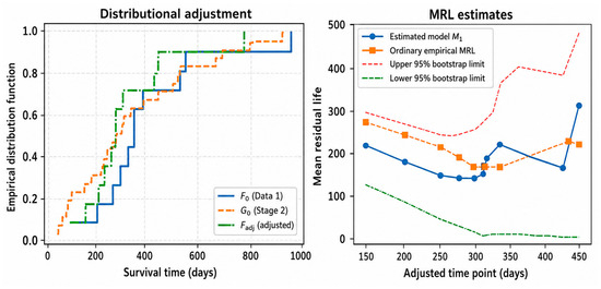
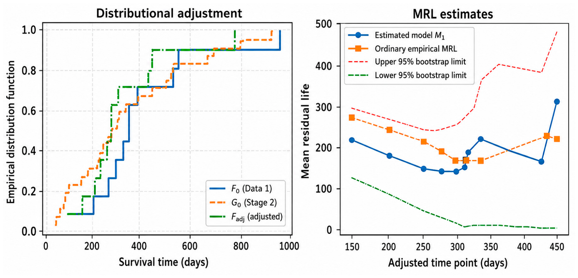
Figure 5 provides a graphical summary of the distributional and residual-life effects of the adjustment. The left panel displays the empirical distribution functions $F_n$ and $G_m$, together with the constraint-adjusted estimator $F_{n,m}^{\ast }$. This panel shows how the adjusted distribution modifies the empirical distribution of Group 1 in order to respect the stochastic precedence relation. The right panel compares the constraint-adjusted MRL estimator $e_{n,m}^{\ast }(x)$ with the ordinary empirical estimator $e_n(x)$, together with the corresponding pointwise $95\%$ bootstrap confidence interval.

Figure 5. (Left) Empirical distribution functions $F_n,G_m$, and the constraint-adjusted estimator $F_{n,m}^{\ast }$. (Right) Constraint-adjusted MRL estimator $e_{n,m}^{\ast }(x)$, ordinary empirical MRL estimator $e_n(x)$, and the corresponding pointwise 95% bootstrap confidence interval. The red and green dotted curves denote the upper and lower confidence limits, respectively.

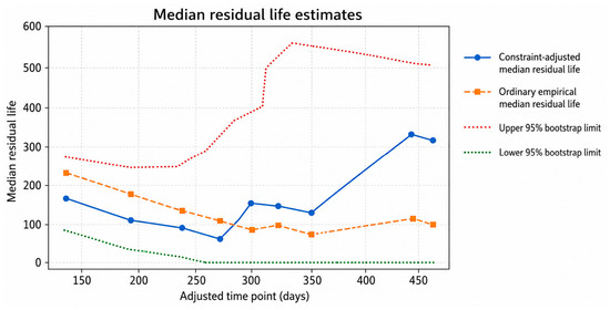
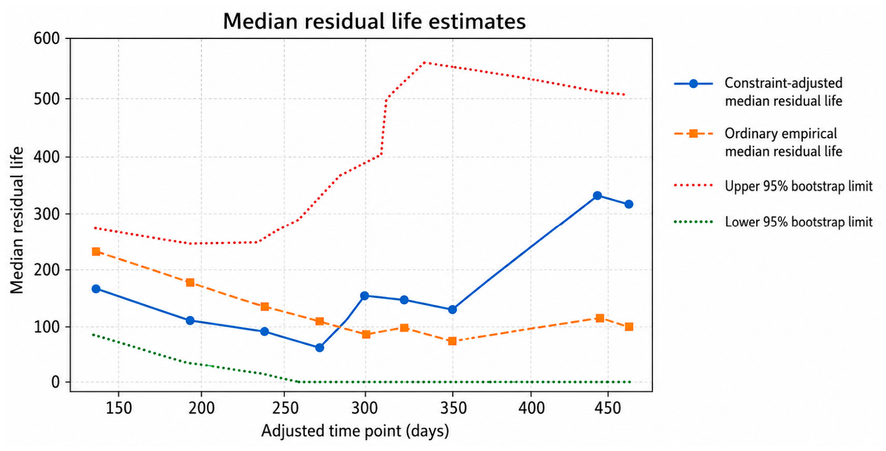
Figure 6 displays the constraint-adjusted median residual-life estimator $q_{0.5,n,m}^{\ast }(x)$, defined in Equation (8), together with the ordinary empirical median residual-life estimator $q_{0.5,n}(x)$ and the corresponding pointwise $95\%$ bootstrap confidence interval.

Figure 6. Constraint-adjusted median residual-life estimator $q_{0.5,n,m}^{\ast }(x)$, ordinary empirical median residual-life estimator $q_{0.5,n}(x)$, and the corresponding pointwise 95% bootstrap confidence interval. The red and green dotted curves denote the upper and lower confidence limits, respectively.

The graphical results show that the adjustment affects both the distributional estimator and the resulting residual-life curves. In particular, the constraint-adjusted estimators provide residual-life profiles that are coherent with the stipulated stochastic precedence direction. The plots also illustrate the sensitivity of ordinary empirical residual-life estimators in regions with limited observations, which is one of the main motivations for introducing a structurally informed adjustment.

5.6. Interpretation and Methodological Implications

The real data analysis illustrates three methodological aspects of the proposed framework. First, it demonstrates how stochastic precedence can be checked empirically through pairwise comparisons before being incorporated into estimation. In the present sample, the unadjusted empirical comparison does not satisfy the clinically motivated direction $X{\le }_{sp}Y$, which makes the example particularly informative: it shows how the proposed estimator enforces a weak structural constraint when the finite sample is not itself compatible with that constraint. Second, the application shows how the constraint-adjusted empirical distribution can be used as a practical input for estimating conditional lifetime functionals. The same adjusted distribution leads to both MRL and median residual-life estimates, showing that the proposed framework is not tied to a single functional but can be applied to different residual-life summaries. Third, the results highlight the finite-sample role of the adjustment. The proposed estimator does not redefine the target MRL or QRL functions. Instead, it evaluates these functionals through an empirical distribution that is compatible with the weak ordering information. This is consistent with the theoretical results in Section 3 and with the Monte Carlo evidence in Section 4, where the adjustment was shown to preserve large-sample validity while improving finite-sample stability.

The application supports the practical relevance of the proposed methodology for structured survival data. It demonstrates that stochastic precedence provides a flexible, interpretable, and empirically assessable mechanism for incorporating partial ordering information into nonparametric residual-life estimation. At the same time, the interpretation remains appropriately cautious: the results highlight the statistical value of the constraint-adjusted procedure and should not be regarded as a standalone clinical conclusion.

6. Conclusions and Future Research

This paper developed a constraint-adjusted nonparametric inference framework for estimating residual-life functionals under stochastic precedence information. The work is positioned within mathematical statistics and nonparametric inference, where a central objective is to construct distribution-free procedures that remain theoretically valid while incorporating meaningful structural information. The motivation arises from comparative reliability and survival studies in which weak directional information between lifetime populations may be available, but stronger assumptions such as usual stochastic ordering or parametric modeling may be difficult to justify. Stochastic precedence provides a natural intermediate structure for this purpose: it is formulated through a pairwise probability condition, does not require pointwise ordering of distribution or survival functions, and can be assessed directly from two-sample data.

The methodological contribution of the paper is the construction of constraint-adjusted estimators for the MRL and QRL functions. The proposed estimators are obtained by applying the MRL and QRL functionals to a constraint-adjusted empirical distribution that enforces stochastic precedence at the sample level. This construction preserves the distribution-free nature of empirical plug-in estimation while incorporating weak ordering information before the residual-life functional is evaluated. Since the adjustment factor is asymptotically negligible, the proposed estimators retain the same population targets as their ordinary empirical counterparts. Under mild regularity conditions, strong consistency is established for both estimators, confirming that the proposed adjustment preserves large-sample validity while adding finite-sample structural coherence.

The numerical results support the practical value of the proposed nonparametric procedure. Across the Weibull and gamma lifetime models, the constraint-adjusted estimators generally exhibited decreasing mean squared error as the sample size increased and frequently improved upon ordinary empirical plug-in estimators, particularly in small and moderate samples. The application to oropharyngeal cancer survival data further illustrates how the method can be implemented in a biomedical setting while maintaining a cautious statistical interpretation. A key practical lesson from the data analysis is that the empirical compatibility of the proposed stochastic precedence direction should be assessed before applying and interpreting the constraint-adjusted estimator. Thus, the proposed framework offers a principled way to combine empirical flexibility, weak stochastic ordering information, and residual-life inference within a single nonparametric methodology.

Several extensions remain open for future work. First, the present paper uses a uniform scaling adjustment to construct the constraint-adjusted estimators. This idea may be extended to more general monotone transformations, which could provide a richer class of constraint-adjusted procedures. Second, deriving the asymptotic distributions of the proposed MRL and QRL estimators would provide a basis for confidence intervals, hypothesis testing, and efficiency comparisons. Third, the same constraint-adjusted principle may be developed for broader classes of conditional lifetime functionals and for other stochastic ordering structures, including hazard rate, likelihood ratio, and dispersive orders, when such assumptions are scientifically plausible and empirically supported. These directions would further expand the role of constraint-adjusted empirical methods in modern nonparametric inference for reliability, survival analysis, and structured lifetime-data modeling. Fourth, extending the framework to right-censored and randomly censored data is an important direction, since censoring is common in survival analysis and complicates both residual-life estimation and empirical assessment of stochastic precedence. For right-censored data, the empirical distribution function may be replaced by the Kaplan–Meier survival estimator, although additional theoretical work would be required to study the resulting constraint-adjusted residual-life estimators.

References

- Gupta, R.C.; Kirmani, S.N.U.A. Some characterization of distributions by functions of failure rate and mean residual life. Commun. Stat.—Theory Methods 2004, 33, 3115–3131. [Google Scholar] [CrossRef] [Scilit]
- Song, J.K.; Cho, G.Y. A note on percentile residual life. Sankhyā Indian J. Stat. Ser. A 1995, 57, 333–335. [Google Scholar]
- Lin, G.D. On the characterization of life distributions via percentile residual lifetimes. Sankhyā Ser. A 2009, 71, 64–72. [Google Scholar]
- Shafaei Noughabi, M.; Franco-Pereira, A.M. Estimation of two ordered quantile residual life functions based on mixtures. J. Stat. Comput. Simul. 2021, 91, 3792–3813. [Google Scholar] [CrossRef] [Scilit]
- Shafaei Noughabi, M.; Franco-Pereira, A.M. Estimation of monotone bivariate quantile residual life. Statistics 2018, 52, 919–933. [Google Scholar] [CrossRef] [Scilit]
- Ghebremichael, M. Nonparametric estimation of mean residual functions. Lifetime Data Anal. 2009, 15, 107–119. [Google Scholar] [CrossRef] [Scilit] [PubMed]
- Zamanzade, E.; Zamanzade, E.; Parvardeh, A. Estimation of a decreasing mean residual life based on ranked set sampling with an application to survival analysis. Int. J. Biostat. 2024, 20, 571–583. [Google Scholar] [CrossRef] [Scilit] [PubMed]
- Arcones, M.A.; Kvam, P.H.; Samaniego, F.J. Nonparametric estimation of a distribution subject to a stochastic precedence constraint. J. Am. Stat. Assoc. 2002, 97, 170–182. [Google Scholar] [CrossRef] [Scilit]
- Finkelstein, M.; Hazra, N.K. Generalization of the pairwise stochastic precedence order to the sequence of random variables. Probab. Eng. Inf. Sci. 2021, 35, 699–707. [Google Scholar] [CrossRef] [Scilit]
- De Santis, E.; Malinovsky, Y.; Spizzichino, F. Stochastic precedence and minima among dependent variables. Methodol. Comput. Appl. Probab. 2021, 23, 187–205. [Google Scholar] [CrossRef] [Scilit]
- van der Vaart, A.W.; Wellner, J.A. Weak Convergence and Empirical Processes: With Applications to Statistics; Springer: New York, NY, USA, 1996. [Google Scholar]
- Abdous, B.; Berred, A. Mean residual life estimation. J. Stat. Plan. Inference 2005, 132, 3–19. [Google Scholar] [CrossRef] [Scilit]
- Csorgo, M.; Csorgo, S. Estimation of percentile residual life. Oper. Res. 1987, 35, 598–606. [Google Scholar] [CrossRef] [Scilit]
- Kalbfleisch, J.D.; Prentice, R.L. The Statistical Analysis of Failure Time Data; Wiley: New York, NY, USA, 1980. [Google Scholar]
Disclaimer/Publisher’s Note: The statements, opinions and data contained in all publications are solely those of the individual author(s) and contributor(s) and not of MDPI and/or the editor(s). MDPI and/or the editor(s) disclaim responsibility for any injury to people or property resulting from any ideas, methods, instructions or products referred to in the content. |
© 2026 by the author. Licensee MDPI, Basel, Switzerland. This article is an open access article distributed under the terms and conditions of the Creative Commons Attribution (CC BY) license.