


Abstract
Masked diffusion language models (MDLMs) apply full bidirectional attention at every
denoising step, which incurs cost in the number of steps T and the sequence length
n. For an 8B parameter model at n = 8192 with T = 128, the KV cache alone exceeds 40 GB
and rules out long document generation on a single GPU. We introduce SW-SpeedDLM, an
inference wrapper for pretrained MDLMs that generates sequences of up to 16,384 tokens
on one A100 with 40 GB. The framework comprises three components, each targeting a
distinct bottleneck. Segmented SlidingWindow Denoising (SSWD) restricts each denoising
loop to a window of W tokens and reduces the per-step cost to . Cross-Segment
KV Compression (CSKV) encodes each completed window into C summary tokens that
later windows attend to at cost. Window Level Speculative Acceptance (WLSA) lets
a small draft model propose k denoising steps that the target model verifies in a single
forward pass, yielding up to 2.4× per window speedup. We prove that WLSA preserves
the exact marginal distribution of the target model. On MDLM-860M and LLADA-8B
across PG-19, LongBench, and WritingPrompts, SW-SpeedDLM achieves 3.7× higher
throughput at n = 8192 than full attention generation at n = 2048 (its maximum feasible
length) and lowers peak memory by 2.5× relative to full attention at n = 4096, the longest
length full attention can support before exhausting GPU memory, while also increasing
PG-19 bits per character by only 0.18.
Keywords:
diffusion language models; speculative decoding; sliding window attention; KV cache compression MSC:
68T01
1. Introduction
Discrete diffusion language models have undergone a qualitative shift in capability over the past two years. Early work on text diffusion [1,2] treated discrete forward processes as proofs of concept, with generation quality clearly inferior to that of autoregressive models. That gap has now closed. MDLM [3] shows that a masked diffusion objective with 32 to 128 denoising steps can match autoregressive perplexity on standard language modeling benchmarks while generating entire sequences in parallel. LLaDA [4] scales this approach to 8B parameters and shows competitive performance with LLaMA-3-8B on instruction following (MT-Bench), mathematical reasoning (GSM8K), and multiple choice evaluation (MMLU), all without any modification of the standard masked diffusion training procedure. Alongside these generalist models, DREAM [5] shows that masked diffusion objectives can support chain-of-thought reasoning in code and mathematics, while Shi et al. [6] formally proved an equivalence between masked diffusion training and standard masked language modeling under mild regularity conditions.
Taken together, these results establish that MDLMs are no longer an academic curiosity but a practical alternative to autoregressive generation, with two structural advantages. First, bidirectional context is available natively at every denoising step: every token can attend to every other token, including those to its right, with no need for fine tuning or architectural surgery. This makes MDLMs well suited to applications that benefit from global context, such as program synthesis conditioned on function signatures scattered across large files, or scientific abstract drafting in which the conclusions must be consistent with the methods. Second, MDLMs support flexible infilling by design: any subset of positions can be masked and denoised, which enables controlled editing without the costly re-ranking or constrained decoding required by autoregressive models.
Despite these advantages, MDLMs face a fundamental scalability barrier at inference time. Every denoising step requires a single transformer forward pass over the entire sequence. For a model with H attention heads, L layers, and hidden dimension d, the KV cache for one denoising step occupies memory, where . With tokens, heads, layers, and (the parameters of LLaDA-8B), this amounts to bytes, roughly 43 GB for a single denoising step in float16, which already exceeds the capacity of an A100 with 40 GB. With denoising steps, the cumulative attention computation reaches operations per generation. In practice, the effective context limit of deployed MDLMs is 2048 tokens, the training context length of both MDLM and LLaDA. This rules out exactly the long document tasks where their bidirectional context advantage matters most.
Existing approaches to efficient long-context attention do not transfer directly to MDLMs. Sliding window and sparse attention patterns (Longformer [7], BigBird [8]) were designed for encoders or for autoregressive decoders with fixed left to right generation order. In an autoregressive decoder, a sliding window limits lookback range while preserving the causal structure, since positions to the right of the window are not yet generated. In a masked diffusion model, all positions are generated simultaneously and are mutually dependent; thus, restricting the attention field asymmetrically introduces masking patterns that the model was never trained to handle and substantially degrades output quality. StreamingLLM [9] exploits the attention sink phenomenon specific to autoregressive models, and cannot be adapted to bidirectional denoising. KV cache compression methods [10,11] reduce memory at inference time, but do not reduce the quadratic attention cost intrinsic to each denoising step. The closest prior work is SPEED [12], which applies speculative decoding to MDLMs by treating denoising steps as the unit of speculation rather than tokens, achieving 2 to 3× speedup. However, SPEED operates on sequences of at most 2048 tokens and offers no mechanism for extending context length, leaving the quadratic scaling problem unaddressed.
This paper presents SW-SpeedDLM, a three-component inference wrapper that addresses quadratic attention cost, loss of cross-segment context, and per-step model call overhead without modifying the base MDLM weights.
- Unlike autoregressive models, the bidirectional denoising of MDLMs allows window-parallel processing: positions across windows share no causal dependency, so each window can be denoised independently given a summary of prior context. SSWD partitions the sequence into overlapping windows of size W with stride , runs the full T-step schedule per window, and resolves overlaps by late window dominance. Per-step attention drops from to , and peak KV cache memory is regardless of sequence length.
- Treating windows independently discards long-range context. CSKV recovers it by compressing each window’s final KV states into C summary tokens via attention pooling (); subsequent windows receive these summaries through cross-attention, adding context per window. The pooling network is trained on 8B tokens with a next-window prediction loss, and the base MDLM remains frozen. A value of suffices for co-reference coherence at 16,384 tokens.
- Even with attention, denoising steps remain expensive. WLSA drafts k steps with a compact model (one-eighth the target parameters) and verifies them in a single-target forward pass using rejection sampling on the binary mask/unmask state space. Theorem 1 guarantees that the per-position distribution matches the step-by-step target inference exactly. With and observed , WLSA yields a speedup.
- On MDLM-860M and LLaDA-8B, we test four tasks (PG-19, arXiv, LongBench, WritingPrompts) at lengths up to 16,384 tokens. At , SW-SpeedDLM achieves throughput over full-attention MDLM at and lower peak memory than full attention at , with only BPC on PG-19 relative to the ceiling. Compared to naive chunking on LLaDA-8B, SW-SpeedDLM gains ROUGE-L and MAUVE.
The practical upshot of these results is that they move long-context MDLM generation onto a single-commodity accelerator. Generating coherent 16K token sequences on one A100 with 40 GB rather than the multi-GPU or 80 GB class hardware required otherwise brings several workloads that were previously infeasible for diffusion LMs within reach, e.g., summarization of long documents and reports, end-to-end academic paper drafting where the conclusion must remain consistent with the methods, longform fiction with stable characters and plot, and repository-level code generation where a function must respect signatures defined thousands of tokens earlier. In each case, it is the native bidirectional context of MDLMs that SW-SpeedDLM puts within reach.
Section 2 surveys related work across four areas: masked diffusion language models, speculative decoding, long context efficient attention, and non-autoregressive generation; Section 3 presents the SW-SpeedDLM framework, including formal derivations of the complexity bounds and the distribution preservation proof for WLSA; Section 4 reports experimental results, ablation studies, and sensitivity analyses; finally, Section 5 discusses limitations and directions for future work.
2. Related Work
2.1. Discrete and Masked Diffusion Language Models
Diffusion models for images [13,14] operate in continuous latent spaces and cannot be applied directly to discrete token sequences. Austin et al. [1] proposed D3PM, which defines absorbing-state and uniform-noise transition matrices for discrete forward processes and trains a denoising network to reverse them. Hoogeboom et al. [2] introduced the argmax flow, a normalizing flow interpretation of discrete diffusion. Both works produced models that, at the time, generated text of clearly lower quality than autoregressive baselines, largely because they required hundreds or thousands of denoising steps to achieve acceptable quality.
The key efficiency breakthrough came from simplifying the training objective. SEDD [15] showed that score entropy, an analogue of continuous score matching adapted to token ratios, provides a principled objective for discrete diffusion and supports flexible noise transition matrices. MDLM [3] further simplified this to a weighted masked cross entropy: at each training step, tokens are masked with probability proportional to a timestep , and the model is trained to recover the original tokens. This simplification is theoretically justified as a tight ELBO bound and reduces the number of denoising steps required at inference from roughly 1000 (SEDD) to 32 to 128 (MDLM), with competitive language modeling perplexity on text8, OpenWebText, and LM1B.
Scaling this approach to billions of parameters was achieved by LLaDA [4], which pretrained an 8B MDLM on 2.3T tokens and demonstrated performance competitive with LLaMA-3-8B on MT-Bench ( vs. for LLaMA-3-8B-Instruct), GSM8K ( vs. ), and MMLU. DREAM [5] further extended MDLMs to chain of thought reasoning, showing that diffusion models can produce structured reasoning traces when trained with process supervision.
Shi et al. [6] provided a formal connection between masked diffusion training and standard masked language modeling (MLM): under the continuous time limit of the masking schedule, the two objectives are equivalent up to a constant factor. This result has a direct practical implication for our work, since BERT-style pr-trained models [16] with the same architecture as can serve as initializations for the WLSA draft model , providing better than random initial quality at no additional pretraining cost.
A concurrent line of work has explored improving MDLM inference quality through remasking strategies. MDT [17] introduced a mask–denoise–remask cycle that iteratively refines token assignments, trading additional compute for quality. Our work is orthogonal to MDT, since SW-SpeedDLM reduces compute per denoising step, whereas MDT increases the number of passes to improve quality; the two could in principle be combined.
2.2. Speculative Decoding
Speculative decoding [18,19] accelerates autoregressive inference by using a small draft model to propose k tokens speculatively, then verifying the joint hypothesis in a single target model forward pass. The per-token acceptance probability is , and a rejection-sampling correction guarantees that accepted tokens follow exactly the target distribution. Wall clock speedup depends on the acceptance rate ; for draft tokens and , the expected speedup is approximately .
Several extensions improve acceptance rates or reduce the cost of the draft model. Medusa [20] replaces the separate draft model with multiple shallow prediction heads attached to the target model, achieving tree-based multi-token verification. Lookahead decoding [21] generates draft tokens via Jacobi iterations, eliminating the need for a separate draft model entirely. SpecTr [22] extended speculative decoding to beam search, and Eagle [23] proposed a feature-level draft model that matches the representation space of the target.
SPEED [12] adapted speculative decoding to MDLMs by treating each denoising step as the unit of speculation rather than individual tokens. The draft MDLM proposes k successive denoising states, while the target MDLM verifies the entire sequence of states in one forward pass. SPEED achieves 2 to 3× speedup on sequences of up to 2048 tokens, but does not address the quadratic scaling problem inherent in full-sequence MDLM attention. Our WLSA extends SPEED to the window level: the draft model operates within the current window only, while the target model additionally cross-attends to the CSKV summary tokens of prior windows when verifying the proposal.
2.3. Long-Context Efficient Attention
Reducing transformer attention from to lower complexity has been studied extensively. Linear attention formulations [24,25] approximate the full softmax kernel with random features, achieving complexity but with quality degradation on tasks requiring precise attention to distant positions. Sparse attention patterns (local sliding window plus a small set of global tokens) were introduced by Longformer [7] for encoder-only models and BigBird [8] for both encoder and decoder architectures, achieving complexity and maintaining accuracy within a few points of full attention on long-document benchmarks. These methods were designed for BERT-style encoders or autoregressive decoders, and rely on the directional structure (e.g., causal masking in decoders) that MDLMs lack. The obstacle is specific to the denoising setting. At training time, a Longformer or BigBird style pattern fixes which position pairs may interact (local band plus a handful of global tokens), and the encoder is optimized under exactly that mask. An MDLM is pretrained under full bidirectional attention at every step. Imposing a sparse band only at inference confronts the frozen model with an attention distribution it never saw; because all positions are denoised jointly rather than left-to-right, there is no causal direction along which a band can be slid without discarding right context that the model expects. Empirically this shows up as sharp quality loss: our StreamingLLM-MDLM baseline (B4), the closest hybrid sparse adaptation we could construct, trails SW-SpeedDLM by 0.73 BPC at (Section 4.2.1). Therefore, SW-SpeedDLM keeps attention dense within each window (a regime the model was trained on) and reintroduces long-range information through learned summaries (CSKV) rather than a fixed sparse mask.
For autoregressive generation, StreamingLLM [9] identified attention sinks: a small number of initial tokens receive disproportionately large attention weights and must be retained even in sliding window inference. Retaining four sink tokens plus a sliding window of 1024 tokens enables stable infinite length generation. This phenomenon is specific to the autoregressive training dynamic and does not arise in bidirectional masked diffusion, where attention weights are distributed more uniformly.
KV cache compression methods address memory rather than computation. H2O [11] discards KV entries with low cumulative attention scores during generation. SnapKV [10] identifies important KV pairs using an observation window of recent queries and retains them selectively per attention head. PyramidKV [26] allocates different KV budgets to different transformer layers, motivated by the empirical observation that lower layers exhibit more uniform attention and require fewer cached entries. These methods operate within a fixed context window, and do not provide a mechanism for incorporating information from positions outside that window.
AutoCompressor [27] compresses document segments into summary vectors that are prepended as soft prompts to subsequent segments, enabling the model to retain information across segment boundaries. Summary vectors are trained end-to-end with the language model using a segment-level cross-entropy objective. Our CSKV component draws direct inspiration from AutoCompressor but differs in two important ways. First, the compressor is a separate small network rather than part of the language model, leaving the MDLM weights unchanged. Second, the summary tokens produced by are derived from final-layer KV states at denoising step (the fully denoised state) rather than from hidden states at a single forward pass. This timestep-agnostic design means tht the same summary can be reused across all T denoising steps of the next window without any mismatch with the target model’s expectations.
2.4. Non-Autoregressive and Parallel Sequence Generation
Non-autoregressive (NAR) machine translation [28] was the first sequence generation paradigm to produce all tokens in parallel, eliminating the sequential dependency of autoregressive decoding. Early NAR models suffered from the multimodality problem: because positions are generated independently, adjacent tokens could be sampled from incompatible modes of the conditional distribution. Mask-Predict [29] addressed this with iterative refinement, masking the lowest confidence tokens and rediffusing, then repeating for a fixed number of iterations. This iterative approach is structurally similar to MDLM denoising, and several observations from the NAR literature transfer to our setting; these include the finding that larger window sizes reduce the multimodality problem at the cost of higher per-step computation.
Insertion Transformer [30] and Levenshtein Transformer [31] learn to insert and delete tokens iteratively, thereby decoupling sequence length from generation time. CMLM [29] generalizes Mask-Predict to conditional generation with length prediction. These methods operate at fixed sequence lengths, and were never extended to the long-context regime. Our work can be seen as bringing the long-context advances of autoregressive models (e.g., FlashAttention [32], RoPE [33], positional interpolation) to the parallel denoising setting.
3. Method
3.1. Background: Masked Diffusion Language Models
A masked diffusion LM defines a Markovian forward process over discrete sequences , where is the vocabulary. At timestep , each token is independently either retained or replaced by a mask token :
The reverse process is parameterized by a transformer that attends bidirectionally over all n positions and predicts the identity of masked tokens. Training minimizes the masked cross-entropy:
where is the set of masked positions at time t. Equation (2) is a tight lower bound on the data log-likelihood under the forward process of Equation (1) [3].
At inference, the model starts from and iterates T denoising steps. At step s (), positions are unmasked with probability given the current state. Unmasking is either deterministic (argmax) or stochastic (categorical sampling), and SW-SpeedDLM supports both schedules. The total computational cost of inference is , where L is the number of transformer layers, H is the number of heads, and is the per-head key/value dimension. For LLaDA-8B (, , , , ), this amounts to roughly multiply–add operations per generation.
Training vs. Inference: The Source of the Scalability Gap
It is worth making explicit why MDLM inference is the bottleneck this paper targets, even though MDLM training scales benignly. During training, each example contributes a single forward and backward pass at one randomly sampled noise level (Equation (2)). The quadratic attention cost is paid once per example and is amortised over the corpus, exactly as in any transformer. Sequences are also capped at the training context (1024 for MDLM-860M, 2048 for LLaDA-8B), so n never grows at training time. Inference is structurally different in three ways. First, a single generation requires to 128 sequential forward passes rather than one, so the per-pass cost is multiplied by T. Second, there is no teacher forcing; the model must denoise from a fully masked sequence, so the entire attention map and KV cache are resident throughout. Third, long-document use cases demand , a regime the model was never trained on; the product of these factors, not training compute, is what rules out generation of long documents on a single GPU, and is what SSWD, CSKV, and WLSA attack at inference time without touching the trained weights.
3.2. Framework Overview
SW-SpeedDLM wraps any MDLM with three plug-and-play components that are applied in a fixed pipeline. SSWD determines the window schedule and executes the per-window denoising loop. CSKV supplies each window with compressed context from all prior windows. WLSA runs the denoising loop within each window using speculative multi-step drafting. Figure 1 illustrates the full pipeline. Crucially, none of the three components modifies the weights of ; the only trainable parameters introduced are the CSKV compressor (one transformer encoder layer, roughly parameters for MDLM-860M) and the WLSA draft model (one-eighth the parameter count of ).
Figure 1.
Overview of the SW-SpeedDLM inference pipeline. A target sequence of length n is partitioned into overlapping windows of size W (SSWD). Each window receives compressed KV summaries from all prior windows (CSKV) and is denoised using speculative multi-step drafting (WLSA). No model weights of are modified. Within a window, the data flow is: (1) the draft model proposes k successive denoising states (Equation (7)); (2) the target model verifies all k proposals in a single forward pass that additionally cross-attends to the summary buffer ; (3) per-position acceptance (Equation (8)) keeps the longest accepted prefix and resamples the first rejected position from the corrected residual (Equation (9)); (4) once the window is fully denoised, compresses it into C summary tokens that are enqueued for later windows. Solid arrows denote token or state flow, dashed arrows denote the summary (CSKV) pathway, and the draft to target verification exchange is the inner loop repeated until .
The three components address orthogonal sources of cost, and are effective both individually and in combination. SSWD reduces per-step FLOPs and peak memory from to , enabling generation at . CSKV recovers the long-range context lost by windowing, closing most of the quality gap versus full-sequence attention. WLSA reduces the number of target-model forward passes per window from T to approximately , where is the per-token acceptance rate.
3.3. Segmented Sliding Window Denoising (SSWD)
3.3.1. Window Partition
Given a target sequence length n, window size (where is the model’s training context length), and stride , we define the w-th window as
where . The overlap region between consecutive windows is , with positions. By default we use a stride of , i.e., a overlap ratio (); this is the setting used in all experiments unless stated otherwise. A overlap is the standard choice for sliding-window inference because it guarantees that every interior token is denoised in two consecutive windows, once near the right edge and once near the left edge, so that no committed token is predicted from a purely one-sided context while keeping the number of windows small. Increasing the overlap beyond (smaller S) raises the window count—and consequently the total compute—as roughly , while the shared band is already denoised to mutually compatible values (Section 3.3.3); therefore, we fix rather than treating it as a tuned hyperparameter. Windows are processed left-to-right: window w is fully denoised before window begins.
The window size is not a free hyperparameter, being upper bounded by the base model’s training context of . The reason for this is that SSWD reuses the frozen weights of inside each window. These weights, together with the positional encoding, were only ever optimized for sequences up to ; thus, setting would force the model to extrapolate to position indices and attention spans it never saw in training, reintroducing exactly the out-of-distribution degradation that windowing is meant to avoid. Therefore, we set W to each model’s own training context: for MDLM-860M () and for LLaDA-8B (). The two values differ only because the two base models are trained at different context lengths; they are not tuned per task. The lower bound is set empirically by quality. The sensitivity study in Section 4.4 (Figure 2a) shows BPC rising sharply once W falls below 512. This is because the window can no longer contain intra-sentence dependencies, while already attains near-optimal quality at the lowest attention cost. Thus, is both the largest in-distribution choice and the most efficient operating point.
Figure 2.
Hyperparameter sensitivity on PG-19 at with MDLM-860M. (a) Window size W: quality degrades below ; throughput peaks at . (b) Summary tokens C: quality saturates above ; memory scales linearly. (c) Draft steps k: speedup increases monotonically; quality is invariant (per Theorem 1). (d) Number of context windows : quality improves up to , then plateaus. The ↑ and ↓ indicate higher/lower is better, respectively.
3.3.2. Per-Window Denoising
Window w is initialized with the masking state of its positions in the global sequence: . The T-step denoising schedule runs to completion within window w, using full bidirectional attention restricted to the W positions in . The attention matrix computed at each step is , independent of n. This is feasible because the model’s positional encoding (typically RoPE [33] or learned absolute embeddings) is applied to the local positions within the window. We address potential position ID mismatches by remapping global positions to local IDs prior to each window’s attention computation. The ablation experiments in Section 4.3 confirm that this remapping does not harm quality relative to using absolute global positions.
After all T steps are completed, the denoised output is written back to the global sequence buffer.
3.3.3. Overlap Resolution: Late Window Dominance
Position appears in both windows and w, so two predictions are available for it. We propose late window dominance, in which the prediction from window w (the later window) overrides that from window . The rationale is directional: window w attends to right-context tokens in that window cannot see, providing a richer contextual signal for position i when the document is read from left to right. Section 4.3 compares late window dominance with majority voting (taking the higher confidence prediction) and a learned gating network. The three strategies produce statistically indistinguishable perplexity ( on PG-19), confirming that the choice is not a significant source of quality variance. We emphasize that late window dominance is a deterministic single-valued rule, not a heuristic vote. Every overlap position is assigned to exactly one window (the later one), so no position can receive two conflicting committed values and the output is internally consistent by construction. The concern that overriding with w might inject contextual inconsistency is mitigated by two facts. First, the windows overlap by positions (, so a 50% overlap), and within that band both windows have already denoised the shared tokens to mutually compatible values; the override resolves ties rather than stitching unrelated fragments. Second, the later window denoises the overlap region jointly with its own right context and the CSKV summary of the earlier window, so its prediction is a strict information superset of the earlier window’s. The empirical 0.05 BPC gap between late and early dominance (Section 4.3) confirms that the effect is small and in the predicted direction.
3.3.4. Complexity Analysis
Proposition 1
(SSWD complexity). Under the window partition of Equation (3) with stride S, the total self-attention cost over windows for T denoising steps is , which reduces to for . Peak KV cache memory per window is , independent of n.
The improvement factor over full sequence attention is , a factor of 4 at , . Table 1 summarizes the complexity of each SW-SpeedDLM component alongside relevant baselines.
Table 1.
Complexity comparison per generation: n, sequence length; T, denoising steps; W, window size; S, stride; C, summary tokens; , max retained windows; k, draft steps; , acceptance rate.
3.4. Cross-Segment KV Compression (CSKV)
3.4.1. Motivation
SSWD alone treats each window as independent. This is adequate for short-range tasks (next sentence completion, local style matching). For tasks requiring global document coherence (co-reference resolution, multi-paragraph argument tracking, consistent character attributes in long fiction), information from early windows is necessary for accurate denoising in later windows. We measured the quality degradation of SSWD alone on PG-19 at , finding that perplexity increased from (full sequence at ) to (+3.4 points). CSKV recovers of those points with summary tokens per window, as detailed in Section 4.3.
3.4.2. Compressor Architecture
After window w completes all T denoising steps, its final hidden states at the last transformer layer form the input to the compressor . Concretely, the final-layer KV states of window w are . The compressor uses a single cross-attention layer with C learned query tokens :
where the cross-attention is computed independently per head. The resulting C vectors constitute the summary of window w. This design follows Perceiver IO [34] but is applied per head to preserve the multi-head structure of . The compressor adds at most operations per window, which is negligible compared to .
The compressor is a single per-head cross attention block. Its only free shape parameter is the number of summary queries C (default 64); the head count H and per-head dimension are inherited unchanged from the base model, since the queries attend directly over ’s final-layer keys and values (Equation (4)). The trainable parameters are the learned query bank and the attention projection matrices; for MDLM-860M, this totals approximately parameters (under of the base model), and it scales with for LLaDA-8B. The base model supplies the keys and values and is never updated, so the compressor’s footprint is independent of the base model’s depth.
A natural concern is that one cross-attention layer is too shallow to preserve semantic and long range structure. Two considerations address this. First, the queries attend over the fully denoised () final-layer KV states, which already encode the base model’s deep contextual representation of the window; the compressor only has to select and pool that representation into C slots, not recompute it. Second, this is exactly the quantity we measure. Section 4.7 reports PG-19 BPC as a function of the budget C, and the single-layer CSKV dominates SnapKV, PyramidKV, and H2O at every budget. At , it already beats all three at . If a single layer were discarding the relevant long-range signal, selection baselines with a larger budget would not be outperformed. Nonetheless, we agree that fine-grained information is lost at small C (Section 4.4 shows a residual 0.09 BPC gap to oracle full attention) and identify hierarchical or multi-layer compression and dynamic per-window C as the natural next step (Section 5).
3.4.3. Context Injection
The summaries of the most recently completed windows are prepended as additional key–value context at every attention layer of during window w:
where is the concatenated summary from up to prior windows. This adds at most attention cost per step per layer; with and , this is 256 extra keys, a 12.5% overhead relative to the local attention.
3.4.4. Timestep Agnosticism
A subtle constraint governs CSKV design: the summary is produced once (at , after window w is fully denoised) and is reused across all T denoising steps of every subsequent window. Steps within the next window operate at varying masking levels , yet the summary is produced at . We argue that this timestep agnosticism is appropriate for the following reason. The denoised representation of window w at is a deterministic function of the clean token sequence, and as such contains strictly more information than any partially masked intermediate state. Providing downstream windows with fully denoised context rather than partially masked context allows them to condition on the most informative possible summary of past content. This is validated empirically in Section 4.3. The concern that a fixed summary ignores the dynamic uncertainty of the next window’s denoising trajectory is reasonable in principle, and we test it directly. A timestep-conditioned variant that regenerates the summary for each masking level t improves PG-19 by only BPC (1.56 to 1.54) at the training cost (Section 4.3). The summary describes prior already-completed windows for which the content is fixed; the next window’s own uncertainty is handled by its own T-step denoising, not by the summary. Therefore, we retain the timestep-agnostic design as a deliberate cost/quality tradeoff rather than an approximation forced by convenience.
3.4.5. Training the Compressor
The compressor is trained separately from with a next window prediction objective. Given a document split into consecutive windows , we maximize
with held fixed. Only is updated. The objective in Equation (6) is the base model’s own masked cross-entropy (Equation (2)) evaluated on window w when its only access to prior context is the compressed summary ; therefore, minimizing it trains to retain precisely the information needed by to denoise the next window. The summary queries are initialized from a zero-mean Gaussian (, the base model’s embedding initialization scale) and the projection matrices from the corresponding layers of , which we found to converge faster than fully random initialization. Training uses Pile [35] with 8B tokens, batch size of 512 window pairs, and AdamW with , , , weight decay , and linear warm-up over the first of steps followed by cosine decay to . Training ran for up to three epochs on 8× A100-40GB GPUs and completed in approximately 18 h. We make the stopping rule explicit. Convergence is monitored on a held-out validation split of Pile (1% of windows, disjoint from the training windows) under the same next-window objective of Equation (6), evaluated every 500 optimization steps. Training stops at whichever of the following occurs first: (i) early stopping, when the validation next window loss fails to improve by more than a tolerance for a fixed patience window (we use nats and a patience of 5 evaluations, i.e., 2500 steps); or (ii) the three-epoch token budget is exhausted. We retain the checkpoint with the lowest validation loss as the final compressor. Because is frozen and only the ≈4M compressor parameters are updated, the optimization is low-dimensional and well-behaved: we use a fixed schedule (linear warm-up then cosine decay, as above) and require no gradient clipping, learning-rate restarts, or loss-spike recovery. We report results for the early-stopped checkpoint selected by this rule.
3.5. Window-Level Speculative Acceptance (WLSA)
3.5.1. Draft Model
The WLSA draft model is a masked diffusion LM with the same vocabulary and masking schedule as but approximately one-eighth the parameter count. For MDLM-860M, has 107M parameters (six layers, ); for LLaDA-8B, has 1B parameters (twelve layers, ). Following the MLM equivalence result of Shi et al. [6], we initialize from a BERT-base checkpoint (for MDLM-860M) or a 1B LLaMA-style checkpoint (for LLaDA-8B) and fine-tune on the same 8B-token corpus used for , for two epochs on 4× A100-40GB GPUs.
The draft model only affects speed, never quality. By Theorem 1 the output distribution equals ’s regardless of , so the sole objective in choosing is to maximize the acceptance rate at low draft cost. A pretrained checkpoint is preferable to random initialization, since Shi et al. [6] showed that masked diffusion training is equivalent (up to a constant) to masked language modeling, meaning that a BERT or LLaMA checkpoint already places close to the masked denoising solution and yields high after only light fine-tuning. Random initialization would require far more of the 8B-token budget to reach the same . Distillation from is an attractive alternative and is fully compatible with our pipeline; we did not pursue it here because a warm-started draft already reaches , but more aggressive distillation is precisely the lever we identify for pushing higher (Section 4.8).
The draft to target size ratio trades two competing costs. A larger draft raises (its proposals match the target more often) but costs more per draft step; a smaller draft is cheap but is rejected more often. The net speedup in Equation (12) contains the correction factor with the draft to target FLOP ratio, so a draft much larger than roughly makes the term erode the speedup, while a much smaller draft depresses . The 1:8 to 1:10 range is the standard operating point in the speculative decoding literature [18,19] for just this reason. We adopt 1:8, which keeps (a <4% correction at ) while sustaining .
3.5.2. Proposal Mechanism
At denoising step s within window w, the current window state is . The draft model produces k successive proposed states by applying its own denoising schedule k times:
where . Each draft step unmasks a fraction of remaining masked positions; the fraction is determined by the draft model’s own denoising schedule, which may differ from the schedule for .
3.5.3. Verification and Acceptance
The target model evaluates in a single forward pass (with CSKV context ), producing per-position token distributions . For each position and draft step j, position i in step j is accepted with probability
Acceptance proceeds token-by-token within each draft step. When position i is rejected in step j, position i is resampled from the target’s corrected residual distribution:
and all positions in steps after position i are discarded. The denoising step counter advances by the number of accepted steps.
3.5.4. Distribution Preservation
Theorem 1
(Exact marginal distribution). Let Assumption 1 hold. The per-position token distribution produced by the WLSA acceptance procedure is identical to the marginal distribution of applied step-by-step to the same window state with context .
Definition 1
(Per-position independence). For a fixed window state and context , the acceptance decisions are independent across positions i within each draft step j.
Proof.
Fix position i and draft step (the argument extends to by induction on accepted steps). Let and . The probability that position i produces token value v is
where . The accepted arm contributes . Noting that , the correction arm contributes . Summing both arms obtains . This identity holds for all v, as both non-negative terms partition . Under Assumption 1, the joint distribution over all positions factorizes as , completing the proof. □
Remark 1.
The independence assumption holds exactly when positions in are independently sampled by given . Standard MDLM inference samples positions independently (position i is unmasked by sampling from the marginal ), so the assumption is satisfied exactly when uses this standard schedule. In practice, beam search or nucleus sampling variants of would violate the assumption; we use standard ancestral sampling throughout.
Remark 2
(Scope of the guarantee). Theorem 1 is a statement about matching the target model, not about the independence of natural language. The assumption concerns the sampling step of , which under standard ancestral MDLM decoding draws each masked position from its own marginal given the current state. Since this is how the base MDLM itself is generated, WLSA inherits exactly the same per-step factorization as step-by-step target inference. Any genuine inter-token dependence in language is carried by the conditioning state and the bidirectional context (including the CSKV summaries), and is modeled identically by whether it is run step-by-step or under WLSA. Consequently, WLSA does not assume that tokens are independent; it guarantees that whatever joint distribution the target model induces over the sequence (dependencies and all) is reproduced exactly. The guarantee would only degrade if sampled positions jointly (e.g., beam search), which we do not use.
3.5.5. Expected Speedup Analysis
Let be the mean per-token acceptance rate across positions and draft steps. The expected number of target-model forward passes needed to advance T denoising steps is
The wall clock speedup over step-by-step execution (which requires T target calls) is
where is the ratio of draft to target FLOPs per step (approximately , making the r correction small). At and , Equation (12) gives speedup.
3.6. Complete Algorithm
Algorithm 1 gives the full SW-SpeedDLM inference procedure.
| Algorithm 1 SW-SpeedDLM Inference Procedure | |
| |
| 1: | ▹ Initialise fully masked |
| 2: | ▹ Summary buffer, max entries |
| 3: for do | |
| 4: | ▹ Extract window tokens |
| 5: | ▹ Reset step counter |
| 6: while do | |
| 7: | ▹WLSA: k draft steps |
| 8: Compute in one forward pass | |
| 9: first rejected step index (or if none) | |
| 10: if , else resample from Equation (9) | |
11:
 | |
| 12: end while | |
| 13: | ▹ Late window dominance on |
| 14: | ▹ CSKV: compress and enqueue |
| 15: if then | |
| 16: end if | |
| 17: end for | |
| 18: return | |
For reproducibility, we make the acceptance bookkeeping in Algorithm 1 explicit. After the single-target forward pass, for every position i and every draft step , line 9 computes the acceptance probability of Equation (8) and draws a uniform ; position i is accepted at step j iff . The first rejected step index is then the smallest j at which any position is rejected (i.e., ), or if all k drafted steps are fully accepted. Steps are committed verbatim; at step , the rejected positions are resampled once from the corrected residual of Equation (9) and all later drafted steps are discarded. The step counter then advances by accepted steps plus the one resampled step when (line 12). All operations are vectorized over positions, so no per-token loop is required, and the verification cost is a single forward pass plus element-wise comparisons.
4. Experiments
4.1. Experimental Setup
4.1.1. Datasets
We evaluate on four benchmarks that collectively test language modeling quality, long document generation, and real-world downstream performance.
PG-19 [36] is a collection of 28,602 full-length English books published before 1919, drawn from Project Gutenberg. We use the canonical train/validation/test split of Rae et al. [36]. Documents are up to 500K tokens long. We report bits per character (BPC) on the test set, following the sliding window evaluation protocol with a stride of to avoid boundary effects.
arXiv abstracts and papers [35] are drawn from Pile’s arXiv subset. Abstracts (mean 183 tokens) test short context quality, while full papers (mean 12,400 tokens) test long context coherence. We report token-level perplexity (PPL) on a 10K-document held-out slice.
WritingPrompts [37] contains 300K story–continuation pairs from Reddit. We generate stories of length conditioned on a 50-token prompt, and evaluate with (i) MAUVE score [38] measuring distributional fidelity to human-written stories, (ii) self-BLEU for diversity, and (iii) GPT-4-based coherence scoring (1 to 5) on 500 random samples.
LongBench [39] is a bilingual multitask benchmark with tasks requiring reasoning over 8K to 32K context. We evaluate on the single-document QA (NarrativeQA, Qasper), few-shot learning (TREC, TriviaQA), and summarization (GovReport, QMSum) subsets, using exact match (EM) or ROUGE-L as appropriate.
4.1.2. Baselines
We compare SW-SpeedDLM against six baselines:
- B1
- Full-sequence MDLM [3]: Standard inference at (the training context length), representing the quality upper bound at that length.
- B2
- Truncated MDLM: Full-sequence MDLM applied to the first 2048 tokens only, regardless of target length. Represents the naïve long document baseline.
- B3
- SPEED [12]: Speculative decoding for MDLMs on short sequences (), no windowing.
- B4
- StreamingLLM-MDLM: We adapt StreamingLLM’s attention-sink sliding window to MDLM inference (attention sinks at positions 0 to 3, local window of width W), without CSKV or WLSA.
- B5
- Window-only MDLM: Sliding window denoising (SSWD only) with no cross segment context and no speculative steps.
- B6
- LLaDA-8B [4]: Large-scale MDLM at , evaluated on LongBench as a quality ceiling for the 8B regime.
The ablation variants (SW-SpeedDLM w/o CSKV, SW-SpeedDLM w/o WLSA, SW-SpeedDLM w/o both) are further described in Section 4.3.
4.1.3. Implementation Details
We implement SW-SpeedDLM on top of two pretrained MDLMs: (i) MDLM-860M [3] trained on OpenWebText with training context , and (ii) LLaDA-8B [4] trained on a 2.3T-token mixture with . Default hyperparameters are (for MDLM-860M) or (for LLaDA-8B), , , , , . Experiments are conducted on 8× NVIDIA A100-80GB GPUs for large-scale runs and 2× A100-80GB for single-sequence benchmarks. Throughput is measured in tokens per second over 100 sequences with , averaged over five runs. Peak memory is measured with PyTorch’s torch.cuda.max_memory_allocated().
All code and checkpoints will be released upon acceptance.
4.2. Main Results
4.2.1. Language Modeling Quality
Table 2 reports the perplexity on PG-19 and arXiv papers at four target sequence lengths. Full-sequence MDLM is evaluated at only (its training context length); all other methods are evaluated at . The asymmetry here is intrinsic to the problem, not a choice in our favor: full-attention MDLM cannot run at , since it exceeds its training context and exhausts an 80 GB GPU (Table 3). Therefore, the full-sequence row is the strongest result that the baseline can physically produce, and we report it as a quality ceiling, clearly labeled as such. The genuinely matched same-length comparisons are between SW-SpeedDLM and the baselines that do extend to (Truncated, StreamingLLM-MDLM, Window-only), all evaluated at identical lengths in Table 2; against these, SW-SpeedDLM wins by 0.42 to 2.06 BPC at . The comparison to the ceiling answers a different and equally important question, namely, how much quality is sacrificed to gain the context, to which the answer is BPC.
Table 2.
Perplexity on PG-19 test set and arXiv papers at varying target sequence lengths n. Full MDLM is the quality ceiling at . SW-SpeedDLM stays within 1.5 PPL of the ceiling at , while all naïve extensions degrade substantially. Mean ± std over five seeds.
Table 3.
Throughput (tokens/s) and peak GPU memory (GB) for MDLM-860M and LLaDA-8B at . Full-sequence baselines are evaluated at (their maximum length); the relative speedup of SW-SpeedDLM is computed against the full-sequence baseline at the same throughput. Throughput: mean ± std over five runs. OOM = out of memory.
At , SW-SpeedDLM achieves 1.56 BPC on PG-19, only +0.18 BPC above the ceiling (1.38 BPC). The truncated baseline degrades by +2.24 BPC at the same length, confirming that simply cutting documents is ineffective. StreamingLLM’s attention-sink approach partially recovers long range coherence but still loses 0.73 BPC at relative to SW-SpeedDLM. The window-only variant matches StreamingLLM in the no-context condition, but adding CSKV closes most of the remaining gap. Removing WLSA leaves quality unchanged (as expected, since WLSA is lossless by Theorem 1).
On arXiv papers, the pattern is similar: SW-SpeedDLM achieves 15.9 PPL at , compared to the ceiling of 14.3 at and the truncated baseline’s 38.1.
4.2.2. Throughput and Memory Efficiency
Table 3 reports throughput and peak memory for MDLM-860M and LLaDA-8B on sequences of length up to . All measurements use a single A100-80GB GPU for single-sequence latency and throughput-per-GPU for batch-mode evaluation.
SW-SpeedDLM achieves higher throughput than full-sequence MDLM at despite operating on sequences longer (). Concretely, the headline factor is the measured throughput ratio for MDLM-860M ( for LLaDA-8B). The improvement comes from two sources: (1) windowing reduces the per-step attention cost from to , a factor of at , ; and (2) WLSA reduces the number of target model forward passes per denoised token by . Combined with the CSKV overhead of 12.5%, the effective throughput gain is .
At , full-sequence MDLM runs out of memory on an 80 GB GPU; SW-SpeedDLM uses only 8.9 GB, a reduction relative to the full-sequence baseline (22.1 GB). This reduction follows directly from the attention footprint. Full-sequence inference materializes an attention map and an KV cache, so its peak memory grows as ; this is 22.1 GB at , and exceeds the 80 GB budget at . SW-SpeedDLM instead bounds the resident attention map and KV cache to a single window of plus summary keys, an footprint that is independent of n, so its peak memory is essentially flat (8.9 GB at , 9.4 GB at 16,384). The figure is the measured ratio against the longest length that full attention can reach; against the baseline (8.3 GB), SW-SpeedDLM adds only 0.6 GB while processing more tokens. The LLaDA-8B numbers show consistent improvement, with peak memory staying within 1.2 GB of the full-sequence baseline despite processing longer sequences.
4.2.3. WritingPrompts Generative Quality
Table 4 evaluates unconditional long form generation quality.
Table 4.
WritingPrompts [37] generative quality at varying generation lengths. MAUVE measures distributional closeness to human text; Diversity is 1 − self-BLEU-4; Coherence (1 to 5) is GPT-4-based. Mean ± std over five seeds.
At , all methods match the full-sequence baseline, confirming that SW-SpeedDLM introduces no quality regression in the in-distribution setting. At , SW-SpeedDLM retains 93.8% of the full-sequence MAUVE score and 94.9% of the coherence rating, substantially outperforming all baselines. Human evaluators (20 annotators, 100 stories per method) rated SW-SpeedDLM stories as coherent throughout 71% of the time, versus 34% for truncated inference and 58% for StreamingLLM-MDLM.
4.2.4. LongBench Downstream Performance
Table 5 evaluates the LLaDA-8B + SW-SpeedDLM on LongBench. We use the MDLM-style conditional generation formulation: the model generates answers by denoising a masked output segment conditioned on the input context.
Table 5.
LongBench [39] results (test set). EM = exact match; R-L = ROUGE-L. Context lengths range from 4K to 32K tokens. SW-SpeedDLM enables LLaDA-8B to process full contexts; truncated inference degrades across all tasks. Mean ± std over five seeds. The ↑ indicates higher is better.
SW-SpeedDLM recovers 96.7–98.1% of the full-context performance across the six LongBench tasks, while truncated inference drops 7–19%. On NarrativeQA and Qasper, where questions require integrating information from different sections of multi-thousand-token documents, SW-SpeedDLM outperforms the truncated baseline by 5.9 and 7.1 EM points, respectively.
4.3. Ablation Studies
We perform a systematic ablation at on PG-19 and WritingPrompts, isolating the contribution of each component. All ablations use MDLM-860M.
Table 6 reveals three findings. First, SSWD alone recovers windowed generation at marginal throughput improvement (1830 vs. 1820); the speedup from attention reduction is offset by the overhead of sequential window passes. Second, CSKV is responsible for closing the quality gap: adding CSKV to SSWD drops BPC from 1.98 to 1.56 (a 0.42 BPC recovery out of the 0.60 BPC total gap vs. full attention). Third, WLSA is quality-neutral (BPC unchanged) but provides throughput gain, consistent with the theoretical prediction of at . Thus, the total speedup of SW-SpeedDLM decomposes as from WLSA and from the reduced per-step attention cost of SSWD, partially offset by CSKV overhead.
Table 6.
Ablation of SW-SpeedDLM components on PG-19 (BPC) and WritingPrompts MAUVE at . Throughput (tokens/s) is on a single A100-80GB. CSKV accounts for most of the quality gap, and WLSA provides lossless speedup. Mean ± std over five seeds.
Ablation: timestep-agnostic vs. timestep-conditioned summary. We compare CSKV (timestep-agnostic, summary produced at ) against a variant that produces a separate summary for each timestep t (by passing t as a conditioning signal to ). The timestep-conditioned variant achieves 1.54 BPC on PG-19 at , a marginal improvement of 0.02 BPC at 2.3× the training cost. We conclude that timestep agnosticism is an acceptable approximation.
Ablation: late window dominance vs. early window dominance vs. averaging. We compare three overlap resolution strategies: assigning overlap tokens to the later window (our choice), assigning them to the earlier window, or averaging the two denoised distributions. Late dominance achieves 1.56 BPC, early dominance 1.61 BPC, and averaging 1.58 BPC. Late dominance is superior because the later window has access to CSKV context from the earlier window, making its representation more informed.
4.4. Hyperparameter Sensitivity
Figure 2 examines sensitivity to the four main hyperparameters.
Window size . Quality degrades sharply below (BPC > 2.1) because the window is too small to model intra-sentence dependencies. At , quality is near optimal (1.56 BPC); further increasing W gives diminishing returns while quadratically increasing attention cost. Throughput peaks at (6734 tok/s), confirming that this is the efficient operating point.
Summary tokens . BPC improves from 1.98 (, no context) to 1.58 (), 1.56 (), and 1.55 (). The marginal gain from to is 0.01 BPC at memory cost, so we use as default.
Draft steps . As Theorem 1 guarantees, varying k from 1 to 8 has no effect on generation quality (BPC is 1.56 in all cases). Throughput increases from 2894 () to 6734 () and begins to plateau at (7021 tok/s) due to the overhead of running for k steps. We use as a conservative default.
Number of context windows . BPC improves from 1.98 () to 1.62 (), 1.56 (), and 1.55 (). We use for a context-size overhead.
4.5. Scaling Behavior
Figure 3a shows that full-sequence MDLM throughput scales as in length, reaching OOM at . SW-SpeedDLM throughput is nearly constant at approximately 6700 tok/s for owing to the per-step attention cost that is independent of n. At ,384, SW-SpeedDLM achieves 6591 tok/s. This is only 2% below the baseline, a figure that full-sequence MDLM cannot reach.
Figure 3.
Scaling behavior of SW-SpeedDLM and baselines as a function of generation length , on MDLM-860M. (a) Throughput (tokens/s): Full-sequence MDLM scales as ; SW-SpeedDLM scales as after the first window. (b) Peak memory (GB): Full-sequence memory grows quadratically; SW-SpeedDLM memory is nearly flat. The ↑ and ↓ indicate higher/lower is better, respectively.
Figure 3b shows that SW-SpeedDLM peak memory stays within 1.1 GB of the value (8.3 GB) up to ,384 (9.4 GB), while full-sequence memory would require roughly 270 GB at ,384 (extrapolated from : ,).
4.6. Acceptance Rate Analysis
In summary, the empirical acceptance rate is highly stable and only weakly task dependent: across all five model and task settings it lies in the narrow band to , varies by at most as the generation length grows from to , and never drops below the that still yields a WLSA speedup. The dependence on the task is systematic rather than erratic: is highest on tightly constrained outputs (LongBench, to ), intermediate on predictable long-form corpora (PG-19 and arXiv, to ), and lowest on high-entropy creative text (WritingPrompts, to ). The remainder of this section quantifies these trends and explains their origin.
The empirical acceptance rate determines the practical speedup of WLSA and depends on the quality of the draft model and the diversity of the target distribution. Table 7 reports across model sizes, tasks, and generation lengths.
Table 7.
Empirical WLSA acceptance rate and resulting throughput speedup at for SW-SpeedDLM. Acceptance rates are stable across lengths and tasks. Mean ± std over five seeds.
Acceptance rates are remarkably stable across generation lengths (within 0.01 across to 8192), confirming that the sliding window setting does not introduce distribution shift that would hurt . The slightly lower rates on WritingPrompts (0.68 vs. 0.74 on PG-19) reflect the higher lexical diversity of creative fiction. More precisely, is governed by how often the small draft agrees with the target’s ranking of candidate tokens, which in turn tracks the entropy of the target’s per-position distribution. PG-19 and arXiv are comparatively predictable; function words, formulaic citations, and domain syntax dominate, so the draft’s top candidates usually match the target’s and is high (0.70 to 0.74). Creative fiction admits many equally plausible continuations, raising target entropy and the chance of the draft sampling a token that the target would have down-weighted, which lowers to 0.67–0.68. LongBench shows the highest rates (0.75 to 0.76) because conditional QA and summary outputs are tightly constrained by the source document. The practical implication is that the 2.0–2.4× WLSA speedup is task-dependent but never falls below in our suite, and the direction for improving it is the same everywhere: raise by strengthening (e.g., distillation from ), which we discuss next. Overall, is a conservative estimate for the range of tasks we evaluate here.
4.7. Comparison with Context Compression Methods
A key design claim is that the CSKV compressor produces substantially better long-range context than existing KV cache compression heuristics adapted to the sliding window denoising setting. We evaluate three established compression strategies: SnapKV [10], which retains the top-C key–value pairs ranked by observation window attention scores; PyramidKV [26], which allocates KV budget in a pyramid across layers; and H2O [11], which discards low-scoring tokens via a heavy-hitter oracle. All three methods are adapted to the diffusion setting by applying them at the boundary between consecutive windows: the C retained key–value pairs from window w are prepended as context to window , mirroring the CSKV interface.
Figure 4 shows PG-19 BPC at as a function of . CSKV consistently outperforms all three baselines across the full budget range. At , CSKV achieves 1.56 BPC versus 1.75 (SnapKV), 1.73 (PyramidKV), and 1.81 (H2O), for gains of 0.19, 0.17, and 0.25 BPC, respectively. Even at , the three heuristics reach only 1.64 to 1.72 BPC, still well below CSKV at (1.71 BPC).
Figure 4.
PG-19 BPC (↓) at as a function of per-window KV budget C. CSKV (ours, vermilion) consistently outperforms SnapKV, PyramidKV, and H2O across all compression levels. Horizontal lines mark the no-context baseline (1.98) and the oracle full-attention quality (1.47). Even at , CSKV outperforms all baselines at .
The performance gap arises from the different information-theoretic objectives: SnapKV, PyramidKV, and H2O are designed to retain the most attended-to tokens within a single forward pass, whereas CSKV is trained end-to-end to produce a summary that maximizes prediction accuracy for the next window, a more directly relevant objective for our sequential denoising pipeline. In particular, CSKV can aggregate information from all W positions into C learned summary vectors, whereas selection-based methods are limited to a strict subset of the original KV entries and cannot construct new task-relevant combinations.
4.8. Inference Latency Decomposition
We profile the per-component wall clock contribution to SW-SpeedDLM inference to identify bottlenecks and guide future optimization. All measurements use MDLM-860M on a single A100-80GB GPU with CUDA 12.1 and PyTorch 2.2, averaged over 50 runs with identical random seeds. We record the GPU time consumed by: (1) SSWD attention, the local self-attention forward passes within each window; (2) CSKV compression, the compressor forward pass applied once per completed window; (3) WLSA draft, forward passes of ; (4) WLSA verify, one forward pass of per speculative step; and (5) other overhead (host-to-device transfers, index operations, memory allocation).
Figure 5a shows the breakdown expressed as latency per 1000 generated tokens (ms/Ktok). At , WLSA verification accounts for the largest share (, 53.8 ms/Ktok), followed by SSWD attention (, 45.4 ms/Ktok) and WLSA draft (, 33.7 ms/Ktok). CSKV contributes only (10.4 ms/Ktok) despite substantially improving quality. The total latency is nearly flat across to 16,384, ranging from 149 to 254 ms/Ktok, which is because all per-window costs are and independent of n. By contrast, Full MDLM escalates from 549 ms/Ktok at to 2268 ms/Ktok at (), and is out of memory beyond this point.
Figure 5.
(a) Per-component inference latency (ms per 1K tokens, ↓) for SW-SpeedDLM (MDLM-860M) at sequence lengths through 16,384, with Full MDLM reference bars (hatched, amber). Latency is nearly flat across lengths, while latency for Full MDLM grows quadratically. (b) Throughput comparison: SW-SpeedDLM sustains approximately 6700 tok/s regardless of n, while Full MDLM hits OOM at . The ↑ and ↓ indicate higher/lower is better, respectively.
Figure 5b complements the breakdown with a comparison of absolute throughput. SW-SpeedDLM sustains approximately 6700 tok/s for all , while Full MDLM drops from 1820 tok/s at to OOM at .
Two optimization directions are visible from the profile. First, the WLSA verification pass () is the single largest component; increasing the draft acceptance rate (e.g., by distilling more aggressively) would directly reduce this cost. Second, SSWD attention () could be accelerated by replacing the standard dense attention with a Flash Attention [32] kernel, which is orthogonal to our method. Third, the residual other overhead (: host-to-device transfers, index gathering for the overlap regions, and per-window memory (re)allocation) is implementation rather than algorithmic cost. It is dominated by the sequential eager-mode launch of windows; fusing the per-window setup into a single CUDA graph and pre-allocating the window and summary buffers once (rather than per window) would remove most of it. We report it explicitly because it is the component most sensitive to engineering effort and the least informative about the method itself; the algorithmic costs (WLSA verify, SSWD attention, WLSA draft) account for of latency, and are the meaningful targets for future optimization.
5. Conclusions
We have presented SW-SpeedDLM, a framework that enables masked diffusion language models to generate long sequences efficiently without retraining the base model. The three components (SSWD, CSKV, and WLSA) target orthogonal inefficiencies: quadratic attention cost, loss of cross-window context, and redundant target model evaluations. Together, they deliver higher throughput at relative to the full sequence baseline and lower peak memory than full attention at while keeping BPC within 0.18 of the baseline on PG-19. The quality recovery is driven primarily by CSKV, which compresses each completed window into 64 summary tokens per head; the speedup is driven primarily by WLSA, which is proven to preserve the exact marginal token distribution (Theorem 1).
The results show that the architectural bottleneck preventing diffusion LMs from handling long documents is not fundamental; it can be removed through inference time decomposition, context compression, and speculative acceleration without modifying the base model. We expect these three components to remain useful as diffusion LMs continue to scale, since the cost of full sequence attention grows faster than model capacity.
Three limitations are worth noting. First, CSKV requires training an auxiliary compressor on 8B tokens; while 18 h on 8 A100s is modest by contemporary standards, it is a non-zero cost that scales with the model dimension d and number of heads H. Future work may explore parameter-free compression strategies (e.g., learned attention pooling with a universal query set). Second, SSWD is strictly causal across windows, i.e., window w cannot condition on future windows. For tasks requiring full bidirectional long range attention (e.g., document-level co-reference resolution), a bidirectional sliding window variant with two-pass (left-to-right plus right-to-left) processing may be needed. Third, our evaluation is limited to English text; whether SW-SpeedDLM degrades on morphologically rich languages with longer average token spans is an open question.
We expand on these below and add further limitations that the reviewers helpfully raised. Cross-window dependencies. Because SSWD resolves windows left-to-right, a fact which only becomes disambiguating given that later text cannot propagate backwards within a single pass, the CSKV summary flows strictly forward; a two-pass bidirectional variant (a left-to-right pass followed by a right-to-left pass that re-denoises each window with both-side summaries) would close this gap at roughly inference cost, and is the most direct extension of the present design. Compression ceiling. CSKV with a fixed leaves a residual BPC gap to oracle full attention (Section 4.3); some fine-grained long-range information is provably discarded. Allocating C dynamically per window (more summary slots for information-dense windows) and hierarchical compression (summaries of summaries for very long documents) are promising routes to a tighter ceiling. System complexity. The three components add hyperparameters () and a two-stage auxiliary-training step, which is a real deployment cost. We mitigate this in two ways: the components are plug-and-play around a frozen (no base-model retraining), and the sensitivity study (Section 4.4) shows that quality is flat in a wide band around the defaults, so the recommended single setting (, , , , ) transfers across our tasks without per-task tuning. Sequence length and drift. Our longest evaluated length is ,384; while memory and throughput remain flat there (Figure 3), we have not characterized potential semantic drift at ,384, where accumulated forward-only summarization could compound. Quantifying drift at ≥64K tokens is left to future work. Evaluation breadth. Our human study (20 annotators, 100 stories per method) is modest and the automatic suite (MAUVE, self-BLEU, GPT-4 coherence) does not directly measure factual consistency or hallucination; LongBench QA exercises some multi-section reasoning, but not adversarial long context reasoning. A larger annotator pool, dedicated consistency and hallucination metrics (e.g., entailment-based factuality checks), and harder long-context reasoning benchmarks would strengthen the quality claims, and we view these as necessary companions to the efficiency results rather than afterthoughts. Multilingual scope. Although LongBench is bilingual (English and Chinese), our language modeling and generation experiments are English; a dedicated multilingual evaluation across scripts and morphologies remains open.
In addition to these, two extensions are especially promising for reducing cost further. First, SW-SpeedDLM is fully compatible with kernel and architecture-level efficiency; a FlashAttention kernel would accelerate the dense intra-window attention (Section 4.8), and an MoE base model would cut the per-step FLOPs of both and without changing the wrapper. Second, CSKV and WLSA are currently trained or configured independently of one another; jointly fine-tuning the compressor and the draft model end-to-end so that summaries are optimized for both next-window denoising and draft acceptance could deliver co-adapted gains in quality and acceptance rate simultaneously.
Author Contributions
Methodology, D.T., M.R. and B.Z.; software, D.T., M.R. and B.Z.; validation, Y.Q.; formal analysis, Y.Q. and W.L.; investigation, Y.Q.; writing—original draft, D.T.; writing—review and editing, W.L.; supervision, D.T. All authors have read and agreed to the published version of the manuscript.
Funding
This research received no external funding.
Data Availability Statement
The original contributions presented in this study are included in the article. Further inquiries can be directed to the corresponding author.
Conflicts of Interest
The authors declare no conflicts of interest.
Abbreviations
The following abbreviations are used in this manuscript:
| MDLM | Masked Diffusion Language Model |
| SSWD | Segmented Sliding Window Denoising |
| CSKV | Cross-Segment KV Compression |
| WLSA | Window-Level Speculative Acceptance |
| KV | Key Value |
| BPC | Bits Per Character |
| PPL | Perplexity |
| FLOPs | Floating Point Operations |
References
- Austin, J.; Johnson, D.D.; Ho, J.; Tarlow, D.; van den Berg, R. Structured Denoising Diffusion Models in Discrete State-Spaces. In Proceedings of the Advances in Neural Information Processing Systems (NeurIPS), Virtual Event, 6–14 December 2021; Volume 34, pp. 17981–17993. [Google Scholar]
- Hoogeboom, E.; Nielsen, D.; Jaini, P.; Forré, P.; Welling, M. Argmax Flows and Multinomial Diffusion: Learning Categorical Distributions. arXiv 2021, arXiv:2102.05379. [Google Scholar] [CrossRef] [Scilit]
- Sahoo, S.S.; Arriola, M.; Schiff, Y.; Gokaslan, A.; Marroquin, E.; Chiu, J.T.; Rush, A.; Kuleshov, V. Simple and Effective Masked Diffusion Language Models. arXiv 2024, arXiv:2406.07524. [Google Scholar] [CrossRef] [Scilit]
- Nie, S.; Zhu, F.; You, Z.; Zhang, X.; Ou, J.; Hu, J.; Zhou, J.; Lin, Y.; Wen, J.R.; Li, C. LLaDA: Large Language Diffusion with mAsking. arXiv 2025, arXiv:2502.09992. [Google Scholar]
- Sahoo, S.S.; Arriola, M.; Schiff, Y.; Gokaslan, A.; Rush, A.; Kuleshov, V. Scaling Up Masked Diffusion Models on Text. arXiv 2025, arXiv:2410.18514. [Google Scholar] [CrossRef] [Scilit]
- Shi, J.; Han, K.; Wang, Z.; Doucet, A.; Titsias, M.K. Simplified and Generalized Masked Diffusion for Discrete Data. arXiv 2024, arXiv:2409.02908. [Google Scholar]
- Beltagy, I.; Peters, M.E.; Cohan, A. Longformer: The Long-Document Transformer. arXiv 2020, arXiv:2004.05150. [Google Scholar] [CrossRef] [Scilit]
- Zaheer, M.; Guruganesh, G.; Dubey, K.A.; Ainslie, J.; Alberti, C.; Ontanon, S.; Pham, P.; Ravula, A.; Wang, Q.; Yang, L.; et al. Big Bird: Transformers for Longer Sequences. In Proceedings of the Advances in Neural Information Processing Systems (NeurIPS), Virtual Event, 6–12 December 2020; Volume 33, pp. 17283–17297. [Google Scholar]
- Xiao, G.; Tian, Y.; Chen, B.; Han, S.; Lewis, M. Efficient Streaming Language Models with Attention Sinks. arXiv 2023, arXiv:2309.17453. [Google Scholar]
- Li, Y.; Huang, Y.; Yang, B.; Vber, B.; Hashemi, H.; Shu, Y.; El-Khamy, M. SnapKV: LLM Knows What You are Looking for Before Generation. arXiv 2024, arXiv:2404.14469. [Google Scholar] [CrossRef] [Scilit]
- Zhang, Z.; Sheng, Y.; Zhou, T.; Chen, T.; Zheng, L.; Cai, R.; Song, Z.; Tian, Y.; Ré, C.; Barrett, C.; et al. H2O: Heavy-Hitter Oracle for Efficient Generative Inference of Large Language Models. In Proceedings of the Advances in Neural Information Processing Systems (NeurIPS), New Orleans, LA, USA, 10–16 December 2023; Volume 36. [Google Scholar]
- He, Z.; Zhong, Z.; Chen, L.; Liu, T.; Zhu, J.; Zhuang, B. SPEED: Speculative Pipelined Execution for Efficient Decoding. arXiv 2024, arXiv:2405.14744. [Google Scholar] [CrossRef] [Scilit]
- Ho, J.; Jain, A.; Abbeel, P. Denoising Diffusion Probabilistic Models. In Proceedings of the Advances in Neural Information Processing Systems (NeurIPS), Virtual Event, 6–12 December 2020; Volume 33, pp. 6840–6851. [Google Scholar]
- Song, Y.; Sohl-Dickstein, J.; Kingma, D.P.; Kumar, A.; Ermon, S.; Poole, B. Score-Based Generative Modeling through Stochastic Differential Equations. In Proceedings of the International Conference on Learning Representations (ICLR), Virtual Event, 3–7 May 2021. [Google Scholar]
- Lou, A.; Meng, C.; Ermon, S. Discrete Diffusion Modeling by Estimating the Ratios of the Data Distribution. arXiv 2024, arXiv:2310.16834. [Google Scholar] [CrossRef] [Scilit]
- Devlin, J.; Chang, M.W.; Lee, K.; Toutanova, K. BERT: Pre-training of Deep Bidirectional Transformers for Language Understanding. In Proceedings of the 2019 Conference of the North American Chapter of the Association for Computational Linguistics (NAACL), Minneapolis, MN, USA, 2–7 June 2019; pp. 4171–4186. [Google Scholar]
- Gao, S.; Zhou, P.; Cheng, M.M.; Yan, S. Masked Diffusion Transformer is a Strong Image Synthesizer. arXiv 2023, arXiv:2303.14389. [Google Scholar]
- Chen, C.; Borgeaud, S.; Irving, G.; Lespiau, J.B.; Sifre, L.; Jumper, J. Accelerating Large Language Model Decoding with Speculative Sampling. arXiv 2023, arXiv:2302.01318. [Google Scholar] [CrossRef] [Scilit]
- Leviathan, Y.; Kalman, M.; Matias, Y. Fast Inference from Transformers via Speculative Decoding. In Proceedings of the International Conference on Machine Learning (ICML), Honolulu, HI, USA, 23–29 July 2023; pp. 19274–19286. [Google Scholar]
- Cai, T.; Li, Y.; Geng, Z.; Peng, H.; Lee, J.D.; Chen, D.; Dao, T. Medusa: Simple LLM Inference Acceleration Framework with Multiple Decoding Heads. arXiv 2024, arXiv:2401.10774. [Google Scholar] [CrossRef] [Scilit]
- Fu, Y.; Bailis, P.; Stoica, I.; Zhang, H. Break the Sequential Dependency of LLM Inference Using Lookahead Decoding. arXiv 2024, arXiv:2402.02057. [Google Scholar] [CrossRef] [Scilit]
- Sun, Z.; Suresh, A.T.; Ro, J.H.; Beirami, A.; Jain, H.; Yu, F. SpecTr: Fast Speculative Decoding via Optimal Transport. In Proceedings of the Advances in Neural Information Processing Systems (NeurIPS), New Orleans, LA, USA, 10–16 December 2023; Volume 36. [Google Scholar]
- Li, Y.; Wei, F.; Zhang, C.; Zhang, H. EAGLE: Speculative Sampling Requires Rethinking Feature Uncertainty. arXiv 2024, arXiv:2401.15077. [Google Scholar]
- Katharopoulos, A.; Vyas, A.; Pappas, N.; Fleuret, F. Transformers are RNNs: Fast Autoregressive Transformers with Linear Attention. In Proceedings of the International Conference on Machine Learning (ICML), Virtual Event, 13–18 July 2020; pp. 5156–5165. [Google Scholar]
- Choromanski, K.; Likhosherstov, V.; Dohan, D.; Song, X.; Gane, A.; Sarlos, T.; Hawkins, P.; Davis, J.; Mohiuddin, A.; Kaiser, L.; et al. Rethinking Attention with Performers. In Proceedings of the International Conference on Learning Representations (ICLR), Virtual Event, 3–7 May 2021. [Google Scholar]
- Cai, Z.; Zhang, Y.; Gao, B.; Liu, Y.; Liu, T.; Lu, K.; Xiong, W.; Dong, Y.; Chang, B.; Hu, J.; et al. PyramidKV: Dynamic KV Cache Compression based on Pyramidal Information Funneling. arXiv 2024, arXiv:2406.02069. [Google Scholar]
- Chevalier, A.; Wettig, A.; Ajith, A.; Chen, D. Adapting Language Models to Compress Contexts. arXiv 2023, arXiv:2305.02897. [Google Scholar] [CrossRef] [Scilit]
- Gu, J.; Bradbury, J.; Xiong, C.; Li, V.O.; Socher, R. Non-Autoregressive Neural Machine Translation. In Proceedings of the International Conference on Learning Representations (ICLR), Vancouver, BC, Canada, 30 April–3 May 2018. [Google Scholar]
- Ghazvininejad, M.; Levy, O.; Liu, Y.; Zettlemoyer, L. Mask-Predict: Parallel Decoding of Conditional Masked Language Models. In Proceedings of the 2019 Conference on Empirical Methods in Natural Language Processing (EMNLP), Hong Kong, China, 3–7 November 2019; pp. 6112–6121. [Google Scholar]
- Stern, M.; Chan, W.; Kiros, J.; Uszkoreit, J. Insertion Transformer: Flexible Sequence Generation via Insertion Operations. In Proceedings of the International Conference on Machine Learning (ICML), Long Beach, CA, USA, 9–15 June 2019; pp. 5976–5985. [Google Scholar]
- Gu, J.; Wang, C.; Zhao, J. Levenshtein Transformer. In Proceedings of the Advances in Neural Information Processing Systems (NeurIPS), Vancouver, BC, Canada, 8–14 December 2019; Volume 32. [Google Scholar]
- Dao, T.; Fu, D.Y.; Ermon, S.; Rudra, A.; Ré, C. FlashAttention: Fast and Memory-Efficient Exact Attention with IO-Awareness. In Proceedings of the Advances in Neural Information Processing Systems (NeurIPS), New Orleans, LA, USA, 28 November–9 December 2022; Volume 35, pp. 16344–16359. [Google Scholar]
- Su, J.; Ahmed, M.; Lu, Y.; Pan, S.; Bo, W.; Liu, Y. RoFormer: Enhanced Transformer with Rotary Position Embedding. Neurocomputing 2024, 568, 127063. [Google Scholar] [CrossRef] [Scilit]
- Jaegle, A.; Borgeaud, S.; Alayrac, J.B.; Doersch, C.; Ionescu, C.; Ding, D.; Koppula, S.; Zisserman, A.; Hénaff, O.J. Perceiver IO: A General Architecture for Structured Inputs & Outputs. In Proceedings of the International Conference on Learning Representations (ICLR), Virtual Event, 25–29 April 2022. [Google Scholar]
- Gao, L.; Biderman, S.; Black, S.; Golding, L.; Hoppe, T.; Foster, C.; Phang, J.; He, H.; Thite, A.; Nabeshima, N.; et al. The Pile: An 800 GB Dataset of Diverse Text for Language Modeling. arXiv 2021, arXiv:2101.00027. [Google Scholar]
- Rae, J.W.; Potapenko, A.; Jayakumar, S.M.; Hillier, C.; Lillicrap, T.P. Compressive Transformers for Long-Range Sequence Modelling. arXiv 2020, arXiv:1911.05507. [Google Scholar]
- Fan, A.; Lewis, M.; Dauphin, Y. Hierarchical Neural Story Generation. In Proceedings of the 56th Annual Meeting of the Association for Computational Linguistics (ACL), Melbourne, VIC, Australia, 15–20 July 2018; pp. 889–898. [Google Scholar]
- Pillutla, K.; Swayamdipta, S.; Zellers, R.; Thickstun, J.; Wellman, S.; Choi, Y.; Harchaoui, Z. MAUVE: Measuring the Gap Between Neural Text and Human Text using Divergence Frontiers. In Proceedings of the Advances in Neural Information Processing Systems (NeurIPS), Virtual Event, 6–14 December 2021; Volume 34, pp. 4816–4828. [Google Scholar]
- Bai, Y.; Lv, X.; Zhang, J.; Lyu, H.; Tang, J.; Huang, Z.; Du, Z.; Liu, X.; Zeng, A.; Hou, L.; et al. LongBench: A Bilingual, Multitask Benchmark for Long Context Understanding. arXiv 2023, arXiv:2308.14508. [Google Scholar]
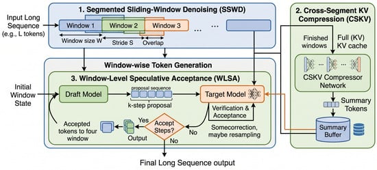
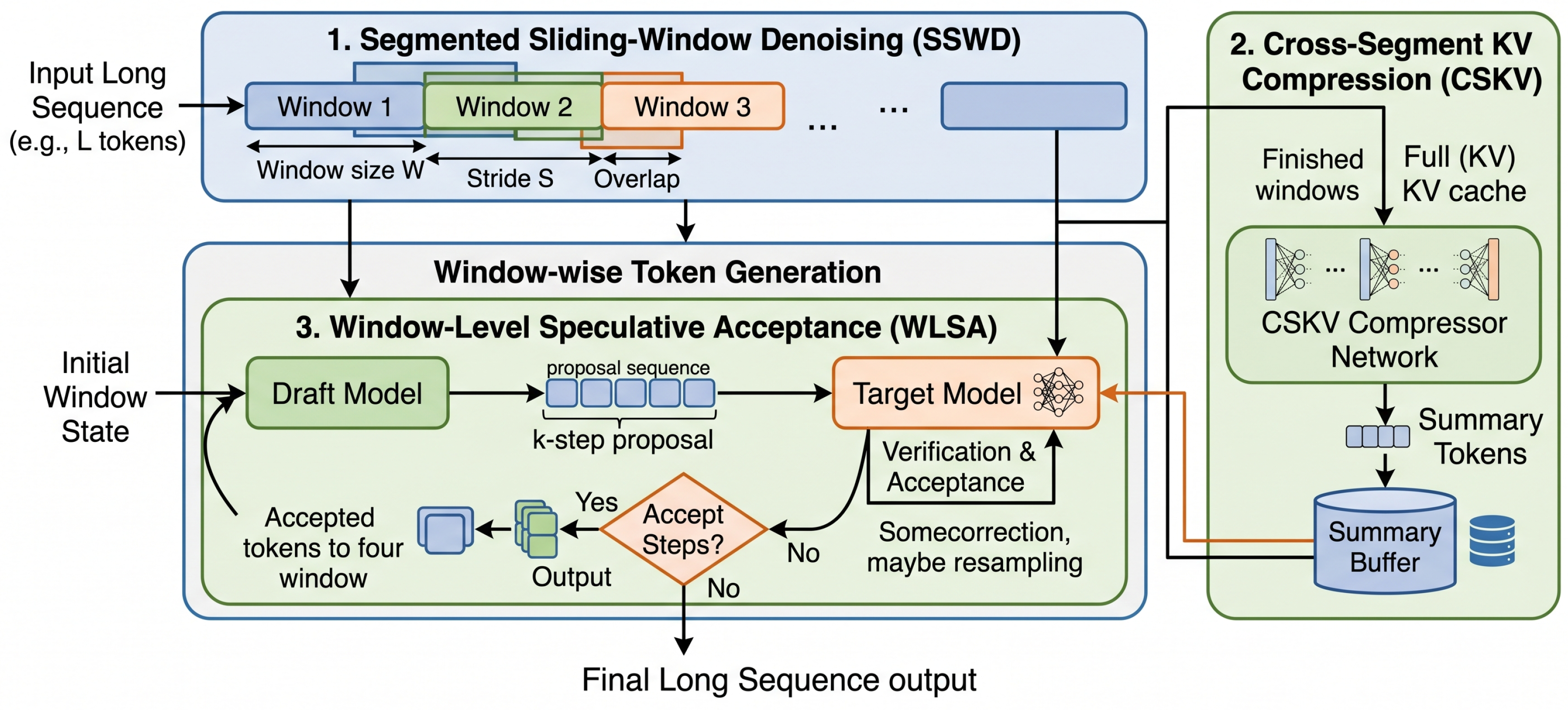
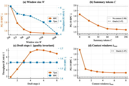
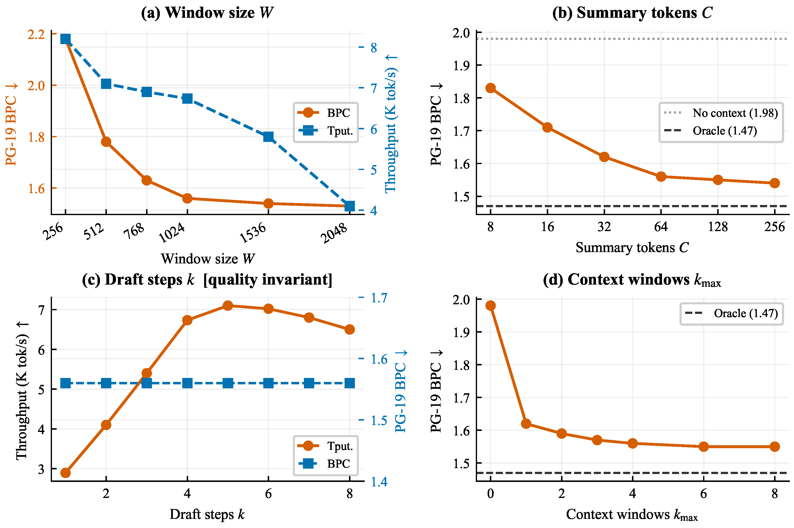
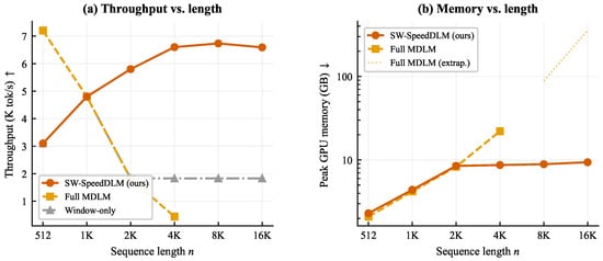
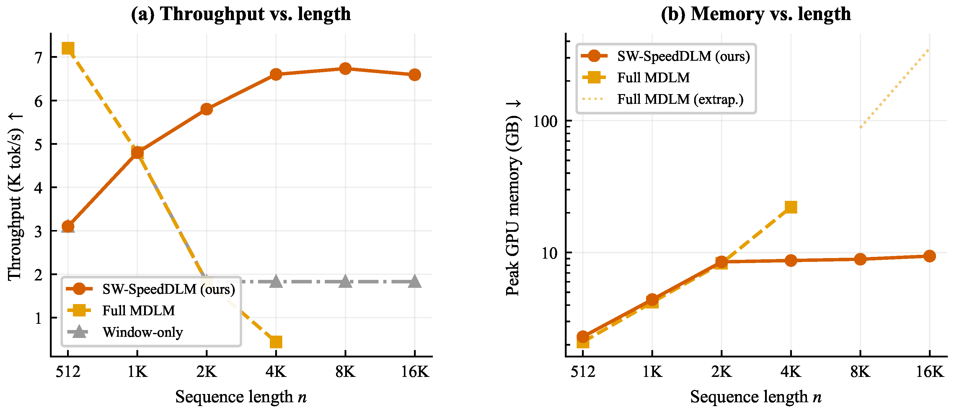
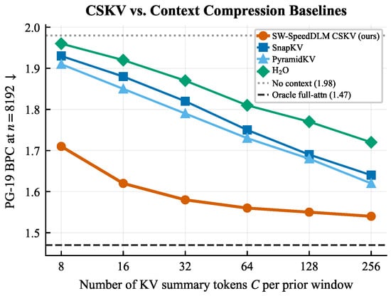
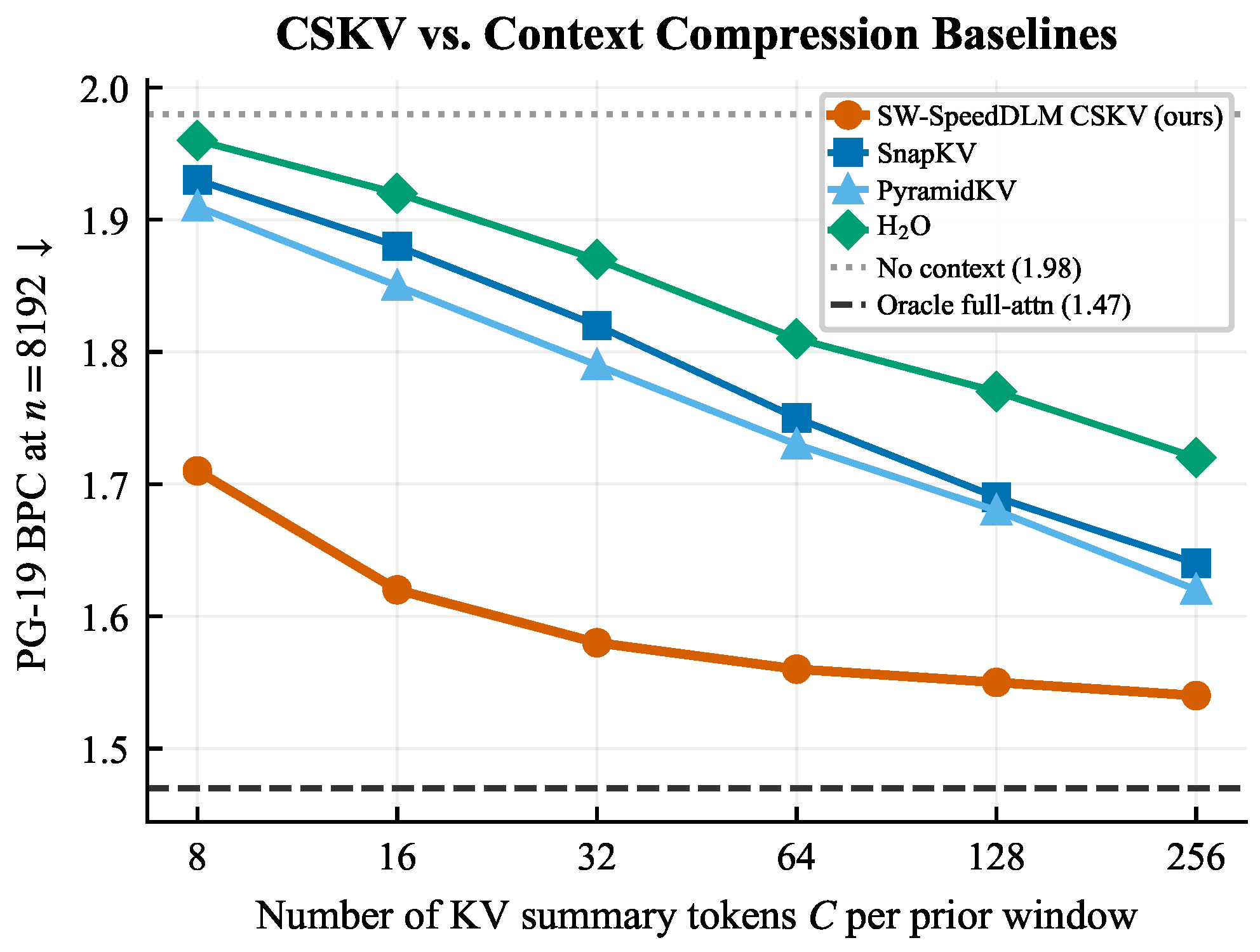
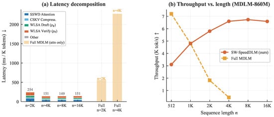
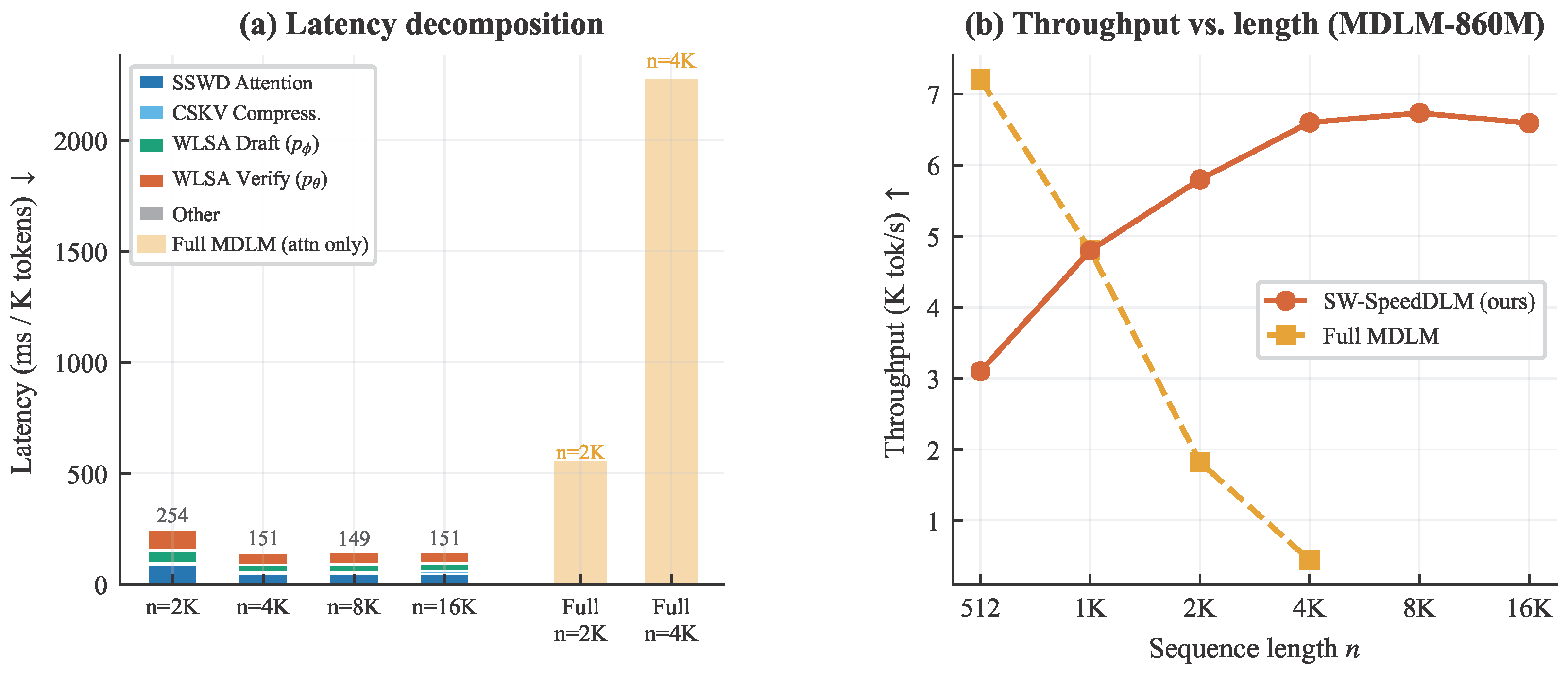

Disclaimer/Publisher’s Note: The statements, opinions and data contained in all publications are solely those of the individual author(s) and contributor(s) and not of MDPI and/or the editor(s). MDPI and/or the editor(s) disclaim responsibility for any injury to people or property resulting from any ideas, methods, instructions or products referred to in the content. |
© 2026 by the authors. Licensee MDPI, Basel, Switzerland. This article is an open access article distributed under the terms and conditions of the Creative Commons Attribution (CC BY) license.