Global Dynamics, Sensitivity Analysis, and Control Strategies for a Delayed Brucellosis Model

Abstract

Brucellosis remains a significant public health and economic burden in many regions, primarily transmitted from livestock to humans through direct contact and environmental contamination. In this paper, we develop a novel cross-species epidemic model that couples the transmission dynamics of brucellosis among sheep, humans, and the environmental reservoir of Brucella. The sheep population is divided into susceptible, exposed, infectious, and vaccinated compartments, while the human population is stratified into susceptible and infected classes. Environmental brucella load is explicitly modeled, and distributed time delays are incorporated to account for incubation periods and delayed exposure risks in humans. We prove that all solutions are non-negative and ultimately bounded, ensuring biological consistency. The basic reproduction number ${\mathcal{R}}_0$ is derived using the next-generation matrix method. Using Lyapunov functionals and LaSalle’s invariance principle, we establish that the disease-free equilibrium is globally asymptotically stable when ${\mathcal{R}}_0\le 1$, whereas a unique endemic equilibrium exists and is globally asymptotically stable when ${\mathcal{R}}_0>1$. Sensitivity analysis identifies the environmental transmission rate, shedding rate, and disinfection as the most influential parameters. Treatment efficacy is shown to exhibit a critical threshold $p^{\mathrm{cr}}=1-1/{\mathcal{R}}_0$, above which eradication becomes feasible. Numerical simulations validate the theoretical findings and demonstrate that time delays affect outbreak timing but not asymptotic stability. These results provide quantitative guidance for brucellosis control strategies, emphasizing environmental sanitation, culling, and vaccination as key interventions.

1. Introduction

Brucellosis is a significant zoonotic disease caused by various species of the genus Brucella. Transmission to humans occurs through multiple routes, including direct contact with infected animals or their secretions, consumption of contaminated water or animal products, and inhalation of infectious aerosols [1]. The disease leads to severe and persistent health issues and economic losses in both animal and human populations [2]. In animals, brucellosis primarily impairs reproductive function and fertility in adults and reduces newborn survival rates [3]. While human mortality is rare, the infection can become chronic and debilitating if not treated promptly [4]. Globally, an estimated 500,000 new human cases occur annually. In mainland China, brucellosis cases emerged in the early 1900s, increased through the 1970s, declined during the 1980s and 1990s, and then rapidly rebounded from 2000 to 2016. Recent evidence indicates another upward trend from 2017 to 2021 [5]. Consequently, developing targeted prevention and control strategies is crucial to suppress this rising trend.

To understand brucellosis transmission dynamics and compare intervention effectiveness, mathematical models have been widely employed. Early models often omitted host population structure or spatial distribution [6,7,8,9,10,11,12]. For instance, Sun and Zhang [11] highlighted the importance of reducing sheep mobility and promoting self-breeding. Liu et al. [10] emphasized vaccination, disinfection, and culling of infected sheep. Gong et al. [6] found that increasing culling and vaccination rates in sheep, alongside health education for humans, reduced prevalence in Ningxia. He et al. [7] showed that shorter delays in intervention lead to lower infection peaks. However, these studies rarely considered heterogeneity in human age groups.

More recent works have incorporated multi-group structures for sheep populations. Li et al. [13] developed a multi-group SEIW model without human population. Yang et al. [14] examined spatial transmission in a two-patch setting. Li et al. [15] studied mixed cross-infection between cattle and sheep. Li et al. [16] included basic ewe and other sheep populations. Qin et al. [17] used a two-patch model for Shanxi and Hebei. Yang et al. [18] incorporated infection age and spatial diffusion. Zheng et al. [19] introduced age-structure in sheep by separating lambs from adults. In [20], the authors develop a cross-species brucellosis model incorporating human age groups, using Jinzhou, China, as a case study. Despite these advances, the delay in brucellosis transmission to humans has rarely been explored as in several diseases [21,22,23,24].

The main contribution of this work is the development and rigorous analysis of a novel cross-species epidemic model that couples brucellosis transmission among sheep, humans, and the environmental reservoir of Brucella. The environmental reservoir $W\left(t\right)$ represents the concentration of viable Brucella bacteria in shared resources (water, soil, feed) that are not directly associated with a live infected animal. This reservoir is maintained by shedding from both exposed and infectious sheep and decays via natural death and disinfection. Unlike previous models, our framework incorporates distributed time delays in human infection pathways, explicit environmental brucella dynamics, and key control interventions including vaccination, culling, and disinfection.

Unlike discrete delays [25], which assume a constant incubation period for all individuals, the distributed delay framework [26,27] captures the inherent heterogeneity in human brucellosis incubation. Clinical evidence indicates that the incubation period of brucellosis in humans can vary from as short as one week to as long as several months, depending on the route of exposure (ingestion, inhalation, or direct contact), the infectious dose, and the individual’s immune status [2,4]. A distributed delay, characterized by a probability density function $\zeta \left(\tau \right)$ over $[0,\omega ]$, allows us to model that different infected individuals become infectious at different times post-exposure. Moreover, the modified kernel $\mathsf{\Pi }\left(\tau \right)=\zeta \left(\tau \right)e^{-n\tau }$ incorporates a decay factor $e^{-n\tau }$ accounting for the progressive loss of bacterial viability over time (e.g., environmental contamination becoming less infectious as it ages). This is particularly relevant for brucellosis, where the pathogen can persist in the environment for extended periods but its infectivity gradually declines. Thus, the distributed delay is not an artificial addition but a biologically motivated feature that improves model fidelity to real-world transmission dynamics.

Using Lyapunov functionals and LaSalle’s invariance principle, we establish the global asymptotic stability of both disease-free and endemic equilibria, showing that the basic reproduction number ${\mathcal{R}}_0$ serves as a sharp threshold parameter. Sensitivity analysis identifies environmental transmission, shedding rate, and disinfection as the most influential factors, while treatment efficacy is shown to exhibit a critical threshold $p^{\mathrm{cr}}=1-1/{\mathcal{R}}_0$ above which eradication becomes feasible. These results provide quantitative, mathematically rigorous guidance for brucellosis control strategies in endemic regions.

Table 1 provides a brief comparison of some recent models with the current one.

Table 1. Comparison of recent brucellosis models with the current one.

Model	Environmental Reservoir	Delay	Global Stability	Sensitivity Analysis	Treatment Threshold
Wang et al. [5]	No	None	No	Yes	No
Gong et al. [6]	No	None	No	Partial	No
He et al. [7]	Yes	Yes	Partial	Yes	No
Liu et al. [10]	No	None	No	Yes	No
Zhang et al. [12]	No	None	Partial	Yes	Partial
Chen et al. [20]	No	None	No	Yes	No
Current model	Yes	Yes	Yes	Yes	Yes

The remainder of this paper is organized as follows. Section 2 presents the formulation of the delayed coupled sheep-human-environment brucellosis model, establishes the non-negativity and boundedness of solutions, and derives the basic reproduction number ${\mathcal{R}}_0$ and the endemic equilibrium. Section 3 proves the global asymptotic stability of the disease-free equilibrium when ${\mathcal{R}}_0<1$ and the global asymptotic stability of the endemic equilibrium when ${\mathcal{R}}_0>1$ using Lyapunov functionals and LaSalle’s invariance principle. Section 4 provides numerical simulations that validate the theoretical results, including sensitivity analysis of ${\mathcal{R}}_0$, evaluation of treatment efficacy thresholds, and investigation of delay effects on human infection dynamics. Section 5 concludes the paper with a discussion of the public health implications and key findings.

2. Mathematical Model Development and Biological Rationale

In this section, we construct a deterministic compartmental framework to capture the transmission dynamics of brucellosis across interconnected populations: sheep, humans, and the environmental reservoir of Brucella bacteria. The model is designed to reflect the key biological features of the disease, including direct transmission among sheep, indirect transmission via contaminated environments, vaccination and culling strategies in livestock, natural mortality, and disease-induced death. For the human population, we additionally incorporate exposure pathways through contact with infected sheep, their carcasses, and environmental brucella, introducing distributed time delays to account for incubation periods and delayed infection risks. Each equation is derived from explicit biological assumptions, such as the equal transmission rates from exposed and infectious sheep, and equal shedding rates from these same compartments. The parameters are defined with clear epidemiological interpretations, ensuring that the model remains both mathematically tractable and practically relevant for public health planning. This formulation provides a rigorous foundation for the analysis of equilibrium stability, threshold dynamics, and intervention strategies.

2.1. Construction of the Coupled Sheep-Human-Brucella Transmission System

In this work, we propose a multi-host epidemic framework to elucidate the transmission mechanisms of brucellosis across species. The total ovine population at time t, denoted $T_1\left(t\right)$, is stratified into four epidemiological classes: susceptible $S_1\left(t\right)$, exposed $E_1\left(t\right)$, infectious $I_1\left(t\right)$, and vaccinated $V_1\left(t\right)$. Brucellosis dissemination within the sheep population occurs via two distinct routes: direct transmission through animal-to-animal contact, and indirect transmission via inhalation of environmental Brucella particles. The quantity $W\left(t\right)$ represents the mean environmental brucella load at time t that is capable of triggering infection. This environmental reservoir represents contaminated soil, animal waste, aborted fetuses, contaminated water, livestock facilities, aerosols, and other environmental media in which Brucella bacteria may survive for extended periods. The environmental compartment $W\left(t\right)$ plays several important epidemiological roles:

(a)

it models indirect transmission pathways beyond direct sheep-to-sheep or sheep-to-human contact;

(b)

it captures the persistence of Brucella bacteria outside the host population;

(c)

it incorporates delayed exposure risks due to environmental contamination;

(d)

it allows evaluation of sanitation and disinfection strategies through the parameter $d_i$;

(e)

it explains how infection may persist even when direct animal contact is reduced.

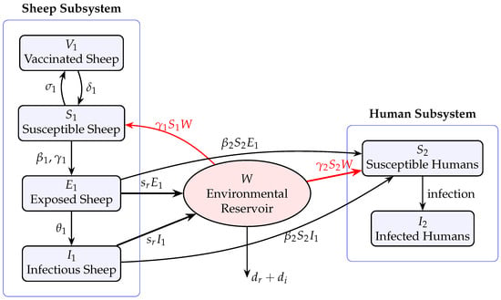
To faithfully capture the coupled dynamics between sheep and their contaminated surroundings (see Figure 1), we invoke the following key assumptions: (i) The direct transmission rate from exposed individuals equals that from infectious individuals when contacting susceptible sheep. (ii) The brucella shedding rates of exposed and infectious sheep are identical.

Figure 1. Schematic representation of the sheep–environment–human brucellosis transmission model.

Under these premises, we formulate the sheep–environment brucella model (1) featuring bilinear incidence, as presented below.

$$\begin{array}{c}\hfill \left\{\begin{array}{c}{\displaystyle \frac{\mathrm{d}{S}_1\left(t\right)}{\mathrm{d}t}}={\Lambda }_1-{\beta }_1{S}_1\left(t\right)(E_1\left(t\right)+I_1\left(t\right))-{\gamma }_1{S}_1\left(t\right)W\left(t\right)+{\delta }_1{V}_1\left(t\right)-{\sigma }_1{S}_1\left(t\right)-m_1{S}_1\left(t\right),\hfill \\ {\displaystyle \frac{\mathrm{d}{E}_1\left(t\right)}{\mathrm{d}t}}={\beta }_1{S}_1\left(t\right)(E_1\left(t\right)+I_1\left(t\right))+{\gamma }_1{S}_1\left(t\right)W\left(t\right)-{\theta }_1{E}_1\left(t\right)-m_1{E}_1\left(t\right),\hfill \\ {\displaystyle \frac{\mathrm{d}{I}_1\left(t\right)}{\mathrm{d}t}}={\theta }_1{E}_1\left(t\right)-{\alpha }_1{I}_1\left(t\right)-{\zeta }_1{I}_1\left(t\right)-m_1{I}_1\left(t\right),\hfill \\ {\displaystyle \frac{\mathrm{d}{V}_1\left(t\right)}{\mathrm{d}t}}={\sigma }_1{S}_1\left(t\right)-{\delta }_1{V}_1\left(t\right)-m_1{V}_1\left(t\right),\hfill \\ {\displaystyle \frac{\mathrm{d}W\left(t\right)}{\mathrm{d}t}}=s_r(E_1\left(t\right)+I_1\left(t\right))-d_{r}W\left(t\right)-d_{i}W\left(t\right),\hfill \end{array}\right.\end{array}$$

(1)

for all $t>0$.

The principal parameters governing sheep population dynamics are interpreted as follows. ${\Lambda }_1$ denotes the recruitment rate; ${\beta }_1$ represents the transmission rate from exposed/infectious sheep to susceptible one; ${\gamma }_1$ is the transmission rate from environmental brucella to susceptible sheep, which means that the term ${\gamma }_1{S}_{1}W$ models indirect ingestion/inhalation from contaminated environment, a critical route for sheep in intensive farming systems where direct contact is limited. ${\sigma }_1$ is the vaccination rate; $m_1$ stands for the natural mortality rate; ${\theta }_1$ is the incubation rate; ${\alpha }_1$ captures the brucellosis-induced mortality rate; and ${\zeta }_1$ signifies the culling rate of infectious sheep. Turning to the environmental brucella compartment, $s_r$ is the brucella shedding rate from exposed and infectious sheep; $d_r$ denotes the natural decay rate of brucella in the environment; and $d_i$ represents the disinfection rate.

The assumption of equal transmission rates from exposed ($E_1$) and infectious ($I_1$) sheep, alongside equal shedding rates from both compartments, represents a common simplification in brucellosis modeling. Hou et al. [8] employed a similar structure in their sheep brucellosis model for Inner Mongolia, treating exposed and infectious animals as collectively contributing to transmission, justified by the observation that Brucella shedding can occur during both the latent and active stages of infection in sheep [3]. This biological rationale is supported by Liu et al. [10], who noted that Brucella excretion may begin during the late incubation period, rendering exposed animals partially infectious [4,8]. However, field data quantifying potential differences in transmission or shedding intensity between $E_1$ and $I_1$ remain scarce. Most serological studies, such as those reviewed by Hou et al., cannot distinguish the timing of exposure relative to infectiousness onset [3,5]. Consequently, the equal-rates assumption, while mathematically tractable and widely adopted, may introduce bias if exposed animals shed substantially fewer bacteria or have lower contact rates than symptomatic infectious animals. In the absence of species-specific empirical estimates differentiating these rates, the model likely captures baseline transmission dynamics but could overestimate the contribution of the exposed class, potentially affecting ${\mathcal{R}}_0$ estimates and the predicted impact of interventions targeting early-stage detection.

We acknowledge the limitation that infectious sheep likely shed more bacteria and present a higher transmission risk than exposed sheep. However, in the absence of quantitative field studies that reliably distinguish shedding rates or contact rates between $E_1$ and $I_1$ for brucellosis in sheep, the equal-rates assumption represents a necessary and conservative simplification. Conservatism here means that if the exposed class is less infectious than assumed, our model overestimates transmission from $E_1$; consequently, any intervention shown to achieve eradication under this more pessimistic scenario would also be effective under a more realistic lower infectiousness of $E_1$. Moreover, the primary aim of this work is the rigorous analytical derivation of threshold conditions (e.g., ${\mathcal{R}}_0$, $p^{\mathrm{cr}}$) rather than precise quantitative prediction for a specific outbreak. The equal-rates assumption maintains mathematical tractability—allowing explicit Lyapunov functional constructions—while still capturing the essential feature that both exposed and infectious sheep contribute to environmental contamination and direct transmission. Future empirical studies should prioritize quantifying differential shedding and transmission rates to refine such models.

Interactions among the human population, sheep population, and environmental brucella are ubiquitous in real-world settings. In this study, we therefore construct a human transmission model in which the total human population $T_2\left(t\right)$ at time t is divided into two compartments: susceptible individuals $S_2\left(t\right)$ and infected individuals $I_2\left(t\right)$. Importantly, infection risk arises not only from exposed and infectious sheep but also from their carcasses, which harbor persistent brucella and are often overlooked despite their significant contribution to human exposure. Susceptible individuals experience losses from three sources: contact with exposed or infectious sheep, contact with carcasses of infected sheep, and exposure to environmental brucella. The transmission rates from exposed sheep, infectious sheep, and their carcasses to susceptible humans are assumed to be identical. Accordingly, we adopt ${\beta }_2{S}_2(E_1+I_1)$ to characterize the loss due to live exposed and infectious sheep, and ${\beta }_2{S}_2\left(m_1{E}_1+({\alpha }_1+m_1)I_1\right)$ to characterize the loss attributable to their carcasses. Based on these formulations, we establish the human delayed differential Equation (2) presented below.

$$\begin{array}{c}\hfill \left\{\begin{array}{ccc}{\displaystyle \frac{\mathrm{d}{S}_2\left(t\right)}{\mathrm{d}t}}\hfill & =\hfill & {\Lambda }_2-{\beta }_2{S}_2\left(t\right)((1+m_1)E_1\left(t\right)+(1+{\alpha }_1+m_1)I_1\left(t\right))\hfill \\ & & -{\gamma }_2{S}_2\left(t\right)W\left(t\right)-m_2{S}_2\left(t\right),\hfill \\ {\displaystyle \frac{\mathrm{d}{I}_2\left(t\right)}{\mathrm{d}t}}\hfill & =\hfill & {\displaystyle {\gamma }_2{\int }_0^{\omega }\mathsf{\Pi }\left(\tau \right)S_2(t-\tau )W(t-\tau )d\tau -m_2{I}_2\left(t\right)}\hfill \\ & & {\displaystyle +{\beta }_2{\int }_0^{\omega }\mathsf{\Pi }\left(\tau \right)S_2(t-\tau )\left((1+m_1)E_1(t-\tau )+(1+{\alpha }_1+m_1)I_1(t-\tau )\right)d\tau ,}\hfill \end{array}\right.\end{array}$$

(2)

for all $t>0$.

In this formulation, ${\Lambda }_2$ denotes the constant recruitment rate of the human population; ${\beta }_2$ represents the direct transmission rate from exposed or infectious sheep to susceptible humans; ${\gamma }_2$ captures the indirect transmission rate from environmental brucella to susceptible humans; and $m_2$ signifies the natural mortality rate of humans. Biological interpretation of all variables and parameters in the distributed-delay model (1)–(2) are provided in Table 2.

Table 2. Biological interpretation of all variables and parameters in the distributed-delay model (1)–(2).

Symbol	Biological Meaning (Units Where Applicable)
$S_1\left(t\right)$	Number of susceptible sheep at time t
$E_1\left(t\right)$	Number of exposed (latent) sheep at time t
$I_1\left(t\right)$	Number of infectious sheep at time t
$V_1\left(t\right)$	Number of vaccinated sheep at time t
$W\left(t\right)$	Average number of Brucella organisms in the environment at time t
$S_2\left(t\right)$	Number of susceptible humans at time t
$I_2\left(t\right)$	Number of infected humans at time t
${\Lambda }_1$	Constant recruitment rate of sheep (births + imports)
${\beta }_1$	Direct transmission rate from exposed/infectious sheep to susceptible sheep
${\gamma }_1$	Indirect transmission rate from environmental Brucella to susceptible sheep
${\sigma }_1$	Vaccination rate of susceptible sheep
$m_1$	Natural mortality rate of sheep
${\theta }_1$	Incubation rate (latent to infectious) in sheep
${\alpha }_1$	Brucellosis-induced mortality rate in sheep
${\zeta }_1$	Culling rate of infectious sheep
${\delta }_1$	Rate of waning vaccine-induced immunity (loss of immunity)
$s_r$	Shedding rate of Brucella by exposed and infectious sheep
$d_r$	Natural decay rate of Brucella in the environment
$d_i$	Disinfection rate (removal of Brucella via sanitation)
${\Lambda }_2$	Constant recruitment rate of humans (births + immigration)
${\beta }_2$	Direct transmission rate from exposed/infectious sheep to susceptible humans
${\gamma }_2$	Indirect transmission rate from environmental Brucella to susceptible humans
$m_2$	Natural mortality rate of humans
$\omega$	Maximum distributed delay (exposure to infection in humans)
$\tau$	Integration variable (time lag) in distributed delay
$\zeta \left(\tau \right)$	Probability density function for distributed delay, defined on $[0,\omega ]$
$\mathsf{\Pi }\left(\tau \right)$	Modified delay kernel defined as $\mathsf{\Pi }\left(\tau \right)=\zeta \left(\tau \right)e^{-n\tau }$, incorporating decay during delay
F	Survival factor ${\displaystyle F={\int }_0^{\omega }\mathsf{\Pi }\left(\tau \right)d\tau }$, satisfies $0<F\le 1$
n	Decay rate in the delay kernel $\mathsf{\Pi }\left(\tau \right)$
${\varphi }_i\left(\theta \right)$	Continuous initial history function for compartment i on $[-\tau ,0]$

Let $T_1\left(t\right)=S_1\left(t\right)+E_1\left(t\right)+I_1\left(t\right)+V_1\left(t\right)$ to be the total population sizes for sheep and $T_2\left(t\right)=S_2\left(t\right)+I_2\left(t\right)$ to be the total population sizes for human.

The system (1) is equipped with known initial values given by continuous functions on $[-\omega ,0]$:

$$S_1\left(\theta \right)={\varphi }_1\left(\theta \right),E_1\left(\theta \right)={\varphi }_2\left(\theta \right),I_1\left(\theta \right)={\varphi }_3\left(\theta \right),V_1\left(\theta \right)={\varphi }_4\left(\theta \right),W\left(\theta \right)={\varphi }_5\left(\theta \right),\theta \in [-\omega ,0]$$

(3)

where ${\varphi }_i\in C([-\omega ,0],{\mathbb{R}}_{+}),i=1,2,\cdots ,5$. The equations describe the dynamics on $t>0$ with initial values given on $[-\omega ,0]$.

The system (2) is equipped with initial values given by continuous functions on the delay interval $[-\omega ,0]$:

$$\begin{array}{c}\hfill S_2\left(\theta \right)={\varphi }_6\left(\theta \right),I_2\left(\theta \right)={\varphi }_7\left(\theta \right),\theta \in [-\omega ,0],\end{array}$$

(4)

where ${\varphi }_6,{\varphi }_7\in C([-\omega ,0],{\mathbb{R}}_{+})$. The equations describe the dynamics on $t>0$ with initial values given on $[-\omega ,0]$.

Let us define the following constants

$$S_1^{in}={\displaystyle \frac{{\Lambda }_1}{m_1}},S_2^{in}={\displaystyle \frac{{\Lambda }_2}{m_2}},{\overline{S}}_1={\displaystyle \frac{S_1^{in}({\delta }_1+m_1)}{({\delta }_1+{\sigma }_1+m_1)}}, \mathrm{a}\mathrm{n}\mathrm{d} {\overline{V}}_1={\displaystyle \frac{S_1^{in}{\sigma }_1}{({\delta }_1+{\sigma }_1+m_1)}}.$$

2.2. Positivity and Ultimate Boundedness of Solutions

To ensure that the proposed brucellosis model is mathematically well-posed and biologically realistic, it is essential to demonstrate that all state variables remain non-negative and bounded for all time $t>0$, given non-negative initial conditions. In this subsection, we prove the positivity of solutions, which guarantees that compartmental populations—susceptible, exposed, infectious, vaccinated sheep, environmental brucella, and susceptible and infected humans—never become negative, preserving their epidemiological interpretation. Furthermore, we prove that all solutions are ultimately bounded, meaning that no population grows indefinitely without bound. This property is biologically plausible due to natural mortality, resource limitations, and disease-induced deaths. The boundedness analysis also defines a positively invariant region $\mathsf{\Omega }$ in the state space, within which all physically meaningful trajectories remain confined. These results lay the groundwork for the subsequent stability analysis and the calculation of the basic reproduction number by ensuring that the model dynamics are confined to a compact domain.

By considering the following set

$$\begin{array}{c}\hfill \begin{array}{c}\mathsf{\Omega }=\left\{\left(S_1,E_1,I_1,V_1,W,S_2,I_2\right)\in {\mathbb{R}}_{+}^7:S_1+E_1+I_1+V_1\le S_1^{in},W\le {\displaystyle \frac{s_r{S}_1^{in}}{(d_r+d_i)}},\right.\hfill \\ \hfill \left.\parallel S_2\parallel \le S_2^{in},\parallel I_2\parallel \le S_2^{in}\right\},\hfill \end{array}\end{array}$$

(5)

we obtain the following results.

Theorem 1

(Non-negativity and Ultimate Boundedness). Trajectories of system (1)–(2) equipped with initial values (3)–(4) are non-negative for all $t\ge 0$. Moreover, all trajectories are ultimately bounded; in particular, there exists a finite time $T>0$ such that for all $t>T$, the trajectory remains within the bounded region Ω. The non-negative orthant ${\mathbb{R}}_{+}^7$ is positively invariant under the flow of the system (1)–(2).

Proof. 

Clearly, ${{\displaystyle \frac{\mathrm{d}{S}_1\left(t\right)}{\mathrm{d}t}}}_{\mid S_1=0}={\Lambda }_1>0$, ${{\displaystyle \frac{\mathrm{d}{E}_1\left(t\right)}{\mathrm{d}t}}}_{\mid E_1=0}={\beta }_1{S}_1{I}_1+{\gamma }_1{S}_{1}W\ge 0$, ${{\displaystyle \frac{\mathrm{d}{I}_1\left(t\right)}{\mathrm{d}t}}}_{\mid I_1=0}={\theta }_1{E}_1\ge 0$, ${{\displaystyle \frac{\mathrm{d}{V}_1\left(t\right)}{\mathrm{d}t}}}_{\mid V_1=0}={\sigma }_1{S}_1\ge 0$, and  ${{\displaystyle \frac{\mathrm{d}W\left(t\right)}{\mathrm{d}t}}}_{\mid W=0}=s_r(E_1+I_1)\ge 0$.

Furthermore, we have

$${\displaystyle \frac{\mathrm{d}{T}_1\left(t\right)}{\mathrm{d}t}}={\Lambda }_1-m_1(S_1\left(t\right)+E_1\left(t\right)+I_1\left(t\right)+V_1\left(t\right))-{\alpha }_1{I}_1\left(t\right)-{\zeta }_1{I}_1\left(t\right)\le {\Lambda }_1-m_1{T}_1\left(t\right).$$

Thus, we get

$$\begin{array}{c}\hfill T_1\left(t\right)\le \left(T_1\left(0\right)-S_1^{in}\right){\mathrm{e}}^{-m_{1}t}+S_1^{in}.\end{array}$$

(6)

Therefore, if $T_1\left(0\right)\le S_1^{in}$ then $T_1\left(t\right)\le S_1^{in}$ for all $t>0$.

Similarly, we prove that $W\left(t\right)$ is bounded as follows:

$$\begin{array}{c}\hfill {\displaystyle \frac{\mathrm{d}W\left(t\right)}{\mathrm{d}t}}\le s_r{S}_1^{in}-(d_r+d_i)W\left(t\right)\end{array}$$

(7)

Thus, we get

$$\begin{array}{c}\hfill W\left(t\right)\le \left(W\left(0\right)-{\displaystyle \frac{s_r{S}_1^{in}}{d_r+d_i}}\right){\mathrm{e}}^{-(d_r+d_i)t}+{\displaystyle \frac{s_r{S}_1^{in}}{d_r+d_i}}.\end{array}$$

(8)

Therefore, if $W\left(0\right)\le {\displaystyle \frac{s_r{S}_1^{in}}{d_r+d_i}}$ then $W\left(t\right)\le {\displaystyle \frac{s_r{S}_1^{in}}{d_r+d_i}}$ for all $t>0$.

According to the first equation of dynamics (2), we get ${\displaystyle \underset{t\to \infty }{lim\; sup}{S}_2\left(t\right)\le {\displaystyle \frac{{\Lambda }_2}{m_2}}=S_2^{in}}$.

Let us define the following:

$$\begin{array}{c}\hfill \begin{array}{c}{\displaystyle \psi \left(t\right)={\int }_0^{\omega }\mathsf{\Pi }\left(\tau \right)S_2(t-\tau )d\tau +I_2\left(t\right).}\hfill \end{array}\end{array}$$

(9)

Then, we obtain the following:

$$\begin{array}{c}\hfill \begin{array}{ccc}{\displaystyle \frac{\mathrm{d}\psi \left(t\right)}{\mathrm{d}t}}\hfill & =\hfill & {\displaystyle {\int }_0^{\omega }\mathsf{\Pi }\left(\tau \right){\displaystyle \frac{\mathrm{d}{S}_2(t-\tau )}{\mathrm{d}t}}d\tau +{\displaystyle \frac{\mathrm{d}{I}_2\left(t\right)}{\mathrm{d}t}}}\hfill \\ & =\hfill & {\displaystyle {\int }_0^{\omega }\mathsf{\Pi }\left(\tau \right)\left[{\Lambda }_2-m_2{S}_2(t-\tau )\right]d\tau -m_2{I}_2\left(t\right)}\hfill \\ & =\hfill & {\displaystyle {\Lambda }_{2}F-m_2\left[{\int }_0^{\omega }\mathsf{\Pi }\left(\tau \right)S_2(t-\tau )d\tau +I_2\left(t\right)\right]}\hfill \\ & =\hfill & {\displaystyle {\Lambda }_2-m_2\psi \left(t\right).}\hfill \end{array}\end{array}$$

(10)

It follows that ${\displaystyle \underset{t\to \infty }{lim\; sup}\psi \left(t\right)={\displaystyle \frac{{\Lambda }_2}{m_2}}=S_2^{in}}$, and then ${\displaystyle \underset{t\to \infty }{lim\; sup}{I}_2\left(t\right)\le S_2^{in}}$. Therefore, we deduce that $\mathsf{\Omega }$ is positively invariant with respect to system (1)–(2).    □

Theorem 1 establishes that the proposed brucellosis model is both mathematically well-posed and epidemiologically meaningful. By proving that every state variable remains non-negative and ultimately bounded for all $t>0$ under biologically realistic initial conditions, we lay a rigorous foundation for the subsequent stability analysis of equilibria and the threshold dynamics governed by the basic reproduction number.

2.3. Equilibrium Characterization and the Basic Reproduction Number

A fundamental step in understanding the long-term behavior of any epidemic model is the identification of steady states and the derivation of the basic reproduction number ${\mathcal{R}}_0$ as a threshold parameter for disease persistence or extinction. In this subsection, we first determine the disease-free equilibrium ${\mathcal{E}}_0$ of the coupled sheep-human-brucella system (1)–(2) by setting all infected compartments to zero and solving the remaining steady-state equations. Subsequently, we compute ${\mathcal{R}}_0$ using the next-generation matrix approach, which linearizes the system around the disease-free equilibrium and isolates the transmission and transition terms associated with the infected states $E_1$, $I_1$, W, and $I_2$. The resulting expression for ${\mathcal{R}}_0$ incorporates contributions from both direct sheep-to-sheep transmission (${\beta }_1$), indirect environmental transmission (${\gamma }_1$), shedding rate ($s_r$), and demographic parameters, as well as the feedback effects from vaccination and culling. Finally, we derive the endemic equilibrium ${\mathcal{E}}^{*}$ under the condition ${\mathcal{R}}_0>1$. The existence of a unique positive endemic equilibrium when the reproduction number exceeds unity is established analytically, providing the necessary groundwork for the global stability analyses presented in Section 3.

Setting the right-hand sides of all equations in models (1)–(2) to zero yields the disease-free equilibrium ${\mathcal{E}}_0=({\overline{S}}_1,0,0,{\overline{V}}_1,0,S_2^{\mathrm{in}},0)$.

Linearizing around the disease-free equilibrium ${\mathcal{E}}_0$ gives the Jacobian matrices

$$\begin{array}{c}\hfill \mathbf{F}=\left(\begin{array}{cccc}{\beta }_1{\overline{S}}_1& {\beta }_1{\overline{S}}_1& {\gamma }_1{\overline{S}}_1& 0\\ 0& 0& 0& 0\\ 0& 0& 0& 0\\ F{\beta }_2{S}_2^{\mathrm{in}}(1+m_1)& F{\beta }_2{S}_2^{\mathrm{in}}(1+{\alpha }_1+m_1)& F{\gamma }_2{S}_2^{\mathrm{in}}& 0\end{array}\right)\end{array}$$

(11)

and

$$\begin{array}{c}\hfill \mathbf{V}=\left(\begin{array}{cccc}{\theta }_1+m_1& 0& 0& 0\\ -{\theta }_1& {\alpha }_1+{\zeta }_1+m_1& 0& 0\\ -s_r& -s_r& d_r+d_i& 0\\ 0& 0& 0& m_2\end{array}\right).\end{array}$$

(12)

Therefore, according to the next-generation matrix method [28], the basic reproduction number of model (1)–(2) is the spectral radius of the matrix $\mathbf{F}{\mathbf{V}}^{-1}$.

$$\begin{array}{c}\hfill \begin{array}{cc}\hfill {\mathcal{R}}_0& =\rho \left(\mathbf{F}{\mathbf{V}}^{-1}\right)\hfill \\ \hfill & ={\displaystyle \frac{{\overline{S}}_1({\theta }_1+{\alpha }_1+{\zeta }_1+m_1)}{({\theta }_1+m_1)({\alpha }_1+{\zeta }_1+m_1)}}\left({\beta }_1+{\displaystyle \frac{{\gamma }_1{s}_r}{d_r+d_i}}\right)\hfill \\ \hfill & ={\displaystyle \frac{{\Lambda }_1({\delta }_1+m_1)({\theta }_1+{\alpha }_1+{\zeta }_1+m_1)}{m_1({\theta }_1+m_1)({\delta }_1+{\sigma }_1+m_1)({\alpha }_1+{\zeta }_1+m_1)}}\left({\beta }_1+{\displaystyle \frac{{\gamma }_1{s}_r}{d_r+d_i}}\right).\hfill \end{array}\end{array}$$

(13)

Let the right-hand side of all equations in models (1)–(2) be zero, and we obtain that the endemic equilibrium point is ${\mathcal{E}}^{*}=(S_1^{*},E_1^{*},I_1^{*},V_1^{*},W^{*},S_2^{*},I_2^{*})$, where

$$\begin{array}{cc}\hfill & S_1^{*}={\displaystyle \frac{({\theta }_1+m_1)({\alpha }_1+{\zeta }_1+m_1)}{({\theta }_1+{\alpha }_1+{\zeta }_1+m_1)}}{\displaystyle \frac{(d_r+d_i)}{{\beta }_1(d_r+d_i)+s_r{\gamma }_1}},E_1^{*}={\displaystyle \frac{{\alpha }_1+{\zeta }_1+m_1}{{\theta }_1}}{I}_1^{*},\hfill \end{array}$$

(14)

$$\begin{array}{cc}\hfill & I_1^{*}={\displaystyle \frac{{\theta }_1{m}_1({\delta }_1+{\sigma }_1+m_1)}{({\delta }_1+m_1)({\theta }_1+{\alpha }_1+{\zeta }_1+m_1)}}{\displaystyle \frac{(d_r+d_i)\left({\mathcal{R}}_0-1\right)}{{\beta }_1(d_r+d_i)+s_r{\gamma }_1}},V_1^{*}={\displaystyle \frac{{\sigma }_1{S}_1^{*}}{{\delta }_1+m_1}},\hfill \end{array}$$

(15)

$$\begin{array}{cc}\hfill & W^{*}={\displaystyle \frac{s_r({\theta }_1+{\alpha }_1+{\zeta }_1+m_1)}{{\theta }_1(d_r+d_i)}}{I}_1^{*},\hfill \end{array}$$

(16)

$$\begin{array}{cc}\hfill & S_2^{*}={\displaystyle \frac{{\Lambda }_2}{{\beta }_2\left((1+m_1)E_1^{*}+(1+{\alpha }_1+m_1)I_1^{*}\right)+{\gamma }_2{W}^{*}+m_2}},\hfill \end{array}$$

(17)

$$\begin{array}{cc}\hfill & I_2^{*}={\displaystyle \frac{{\beta }_2\left((1+m_1)E_1^{*}+(1+{\alpha }_1+m_1)I_1^{*}\right)+{\gamma }_2{W}^{*}}{m_2}}F{S}_2^{*}.\hfill \end{array}$$

(18)

If ${\mathcal{R}}_0>1$, then $I_1^{*}>0$. We further obtain $E_1^{*}>0$ and $W^{*}>0$. Since $S_1^{*}>0$, we further derive $V_1^{*}>0$. The substitution gives that $S_2^{*}>0$, and $I_2^{*}>0$. So, a unique endemic equilibrium point exists.

3. Global Dynamics and Threshold Behavior

Having established the biological soundness of the model and derived the basic reproduction number ${\mathcal{R}}_0$, we now investigate the long-term dynamical behavior of the brucellosis transmission system. The stability properties of the disease-free equilibrium ${\mathcal{E}}_0$ and the endemic equilibrium ${\mathcal{E}}^{*}$ are analyzed using Lyapunov functional methods combined with LaSalle’s invariance principle. This section demonstrates that ${\mathcal{R}}_0$ serves as a sharp threshold parameter: when ${\mathcal{R}}_0<1$, the disease-free equilibrium is globally asymptotically stable, indicating that brucellosis inevitably dies out irrespective of initial conditions. Conversely, when ${\mathcal{R}}_0>1$, the disease-free equilibrium becomes unstable, and a unique endemic equilibrium emerges and attracts all positive solutions, signifying persistent disease circulation. The Lyapunov functions constructed here exploit the specific nonlinear structure of the model and incorporate the delay effects arising from human exposure pathways. These results provide a rigorous mathematical foundation for evaluating control strategies and predicting outbreak outcomes under different epidemiological scenarios.

Define H to be the function $\mathsf{\Theta }\left(Z\right)=Z-1-lnZ$, for $Z>0$ that has the following essential properties: (i) $\mathsf{\Theta }\left(Z\right)\ge 0$ for all $Z>0$, with equality if and only if $Z=1$; (ii) $\mathsf{\Theta }$ attains its unique global minimum at $Z=1$, where $\mathsf{\Theta }\left(1\right)=0$; (iii) ${\displaystyle \underset{Z\to 0^{+}}{lim}\mathsf{\Theta }\left(Z\right)=\underset{Z\to \infty }{lim}\mathsf{\Theta }\left(Z\right)=+\infty }$; and (iv) ${\displaystyle \frac{d\mathsf{\Theta }\left(Z\right)}{dZ}}=1-{\displaystyle \frac{1}{Z}}$. This form is extensively used to construct Lyapunov functionals to prove global asymptotic stability, as we will do in this section.

Theorem 2.

If ${\mathcal{R}}_0\le 1$, then the disease-free equilibrium point ${\mathcal{E}}_0$ is globally asymptotically stable.

Proof. 

To prove the global asymptotic stability of the disease-free equilibrium ${\mathcal{E}}_0$ when ${\mathcal{R}}_0\le 1$, we first construct a Lyapunov functional ${\mathcal{F}}_1$ that combines a weighted sum of the infected compartments with suitable nonlinear terms for the susceptible and vaccinated sheep populations. The proof is done in several steps.

The disease-free equilibrium point of model (1) is ${\mathcal{E}}_0^s=({\overline{S}}_1;0;0;{\overline{V}}_1;0)$. Define a Lyapunov function

$$\begin{array}{c}\hfill {\mathcal{F}}_1={\overline{S}}_1\mathsf{\Theta }\left({\displaystyle \frac{S_1}{{\overline{S}}_1}}\right)+{\overline{V}}_1\mathsf{\Theta }\left({\displaystyle \frac{V_1}{{\overline{V}}_1}}\right)+E_1+{\displaystyle \frac{\left({\beta }_1{\overline{S}}_1(d_r+d_i)+s_r{\gamma }_1{\overline{S}}_1\right)}{(d_r+d_i)({\alpha }_1+{\zeta }_1+m_1)}}{I}_1+{\displaystyle \frac{{\gamma }_1{\overline{S}}_1}{d_r+d_i}}W.\end{array}$$

(19)

Taking the derivative of ${\mathcal{F}}_1$, by using the equalities for ${\mathcal{E}}_0^s$, that ${\Lambda }_1=({\sigma }_1+m_1){\overline{S}}_1-{\delta }_1{\overline{V}}_1$ and ${\sigma }_1{\overline{S}}_1=({\delta }_1+m_1){\overline{V}}_1$, we obtain

$$\begin{array}{c}\hfill \begin{array}{ccc}{\displaystyle \frac{\mathrm{d}{\mathcal{F}}_1}{\mathrm{d}t}}\hfill & =\hfill & \left(1-{\displaystyle \frac{{\overline{S}}_1}{S_1}}\right){\dot{S}}_1+\left(1-{\displaystyle \frac{{\overline{V}}_1}{V_1}}\right){\dot{V}}_1+{\dot{E}}_1+{\displaystyle \frac{\left({\beta }_1{\overline{S}}_1(d_r+d_i)+s_r{\gamma }_1{\overline{S}}_1\right)}{(d_r+d_i)({\alpha }_1+{\zeta }_1+m_1)}}{\dot{I}}_1+{\displaystyle \frac{{\gamma }_1{\overline{S}}_1}{d_r+d_i}}\dot{W}\hfill \\ & =\hfill & \left(1-{\displaystyle \frac{{\overline{S}}_1}{S_1}}\right)\left({\Lambda }_1-{\beta }_1{S}_1(E_1+I_1)-{\gamma }_1{S}_{1}W+{\delta }_1{V}_1-{\sigma }_1{S}_1-m_1{S}_1\right)\hfill \\ & & +\left(1-{\displaystyle \frac{{\overline{V}}_1}{V_1}}\right)\left({\sigma }_1{S}_1-{\delta }_1{V}_1-m_1{V}_1\right)+\left({\beta }_1{S}_1(E_1+I_1)+{\gamma }_1{S}_{1}W-{\theta }_1{E}_1-m_1{E}_1\right)\hfill \\ & & +{\displaystyle \frac{\left({\beta }_1{\overline{S}}_1(d_r+d_i)+s_r{\gamma }_1{\overline{S}}_1\right)}{(d_r+d_i)({\alpha }_1+{\zeta }_1+m_1)}}\left({\theta }_1{E}_1-({\alpha }_1+{\zeta }_1+m_1)I_1\right)+{\displaystyle \frac{{\gamma }_1{\overline{S}}_1}{d_r+d_i}}\left(s_r(E_1+I_1)-(d_r+d_i)W\right)\hfill \\ & =\hfill & \left(1-{\displaystyle \frac{{\overline{S}}_1}{S_1}}\right)\left(({\sigma }_1+m_1){\overline{S}}_1-{\delta }_1{\overline{V}}_1-{\beta }_1{S}_1(E_1+I_1)-{\gamma }_1{S}_{1}W+{\delta }_1{V}_1-{\sigma }_1{S}_1-m_1{S}_1\right)\hfill \\ & & +\left(1-{\displaystyle \frac{{\overline{V}}_1}{V_1}}\right)\left(({\delta }_1+m_1){\overline{V}}_1{\displaystyle \frac{S_1}{{\overline{S}}_1}}-{\delta }_1{V}_1-m_1{V}_1\right)+\left({\beta }_1{S}_1(E_1+I_1)+{\gamma }_1{S}_{1}W-{\theta }_1{E}_1-m_1{E}_1\right)\hfill \\ & & +{\displaystyle \frac{\left({\beta }_1{\overline{S}}_1(d_r+d_i)+s_r{\gamma }_1{\overline{S}}_1\right)}{(d_r+d_i)({\alpha }_1+{\zeta }_1+m_1)}}\left({\theta }_1{E}_1-({\alpha }_1+{\zeta }_1+m_1)I_1\right)+{\displaystyle \frac{{\gamma }_1{\overline{S}}_1}{d_r+d_i}}\left(s_r(E_1+I_1)-(d_r+d_i)W\right)\hfill \\ & =\hfill & m_1{\overline{S}}_1\left(2-{\displaystyle \frac{S_1}{{\overline{S}}_1}}-{\displaystyle \frac{{\overline{S}}_1}{S_1}}\right)+m_1{\overline{V}}_1\left(3-{\displaystyle \frac{{\overline{S}}_1}{S_1}}-{\displaystyle \frac{V_1}{{\overline{V}}_1}}-{\displaystyle \frac{S_1{\overline{V}}_1}{{\overline{S}}_1{V}_1}}\right)+{\delta }_1{\overline{V}}_1\left(2-{\displaystyle \frac{{\overline{S}}_1{V}_1}{S_1{\overline{V}}_1}}-{\displaystyle \frac{S_1{\overline{V}}_1}{{\overline{S}}_1{V}_1}}\right)\hfill \\ & & +({\theta }_1+m_1)({\mathcal{R}}_0-1)E_1.\hfill \end{array}\end{array}$$

Since $x_1+x_2+\cdots +x_n\ge n\sqrt[n]{x_1{x}_2\dots x_n}$ for $x_1\ge 0,x_2\ge 0,\dots ,x_n\ge 0$, we obtain that

$$\begin{array}{c}\hfill 2-{\displaystyle \frac{S_1}{{\overline{S}}_1}}-{\displaystyle \frac{{\overline{S}}_1}{S_1}}\le 0,3-{\displaystyle \frac{{\overline{S}}_1}{S_1}}-{\displaystyle \frac{V_1}{{\overline{V}}_1}}-{\displaystyle \frac{S_1{\overline{V}}_1}{{\overline{S}}_1{V}_1}}\le 0,2-{\displaystyle \frac{{\overline{S}}_1{V}_1}{S_1{\overline{V}}_1}}-{\displaystyle \frac{S_1{\overline{V}}_1}{{\overline{S}}_1{V}_1}}\le 0.\end{array}$$

(20)

If ${\mathcal{R}}_0\le 1$, it then follows that ${\displaystyle \frac{\mathrm{d}{\mathcal{F}}_1}{\mathrm{d}t}}\le 0$. For ${\displaystyle \frac{\mathrm{d}{\mathcal{F}}_1}{\mathrm{d}t}}=0$, we derive that $S_1={\overline{S}}_1$, $V_1={\overline{V}}_1$, and $E_1=0$. Let ${\mathsf{\Omega }}_1=\{(S_1;E_1;I_1;V_1;W)\in {\mathbb{R}}_{+}^5|{\displaystyle \frac{\mathrm{d}{\mathcal{F}}_1}{\mathrm{d}t}}=0\}=\{{\mathcal{E}}_0^s=({\overline{S}}_1;0;0;{\overline{V}}_1;0)\}$. By substituting $S_1={\overline{S}}_1$, $V_1={\overline{V}}_1$, and $E_1=0$ into model (1), we obtain that $I_1=0$ and $W=0$. Thus, $\left\{{\mathcal{E}}_0^s\right\}$ is the largest invariant set in ${\mathsf{\Omega }}_1$. According to LaSalle’s Invariant Principle, ${\mathcal{E}}_0^s$ is globally asymptotically stable.

We substitute the disease-free equilibrium point ${\mathcal{E}}_0^s$ into model (2), and derive

$$\begin{array}{c}\hfill \left\{\begin{array}{c}{\displaystyle \frac{\mathrm{d}{S}_2}{\mathrm{d}t}}={\Lambda }_2-m_2{S}_2,\hfill \\ {\displaystyle \frac{\mathrm{d}{I}_2}{\mathrm{d}t}}=-m_2{I}_2.\hfill \end{array}\right.\end{array}$$

(21)

The disease-free equilibrium point of model (21) is ${\mathcal{E}}_0^h=(S_2^{in};0)$. Define a Lyapunov function

$$\begin{array}{c}\hfill {\mathcal{F}}_2=S_2^{in}\mathsf{\Theta }\left({\displaystyle \frac{S_2}{S_2^{in}}}\right)+I_2.\end{array}$$

(22)

Taking the derivative of ${\mathcal{F}}_2$, we obtain

$$\begin{array}{c}\hfill {\displaystyle \frac{\mathrm{d}{\mathcal{F}}_2}{\mathrm{d}t}}=-{\displaystyle \frac{m_2}{S_2}}{\left(S_2-S_2^{in}\right)}^2-m_2{I}_2.\end{array}$$

(23)

Therefore, it then follows that ${\displaystyle \frac{\mathrm{d}{\mathcal{F}}_2}{\mathrm{d}t}}\le 0$. For ${\displaystyle \frac{\mathrm{d}{\mathcal{F}}_2}{\mathrm{d}t}}=0$, we obtain $S_2=S_2^{in}$ and $I_2=0$. Let ${\mathsf{\Omega }}_2=\{(S_2,I_2)\in {\mathbb{R}}_{+}^2|{\displaystyle \frac{\mathrm{d}{\mathcal{F}}_2}{\mathrm{d}t}}=0\}=\{{\mathcal{E}}_0^h=(S_2^{in},0)\}$. Thus, $\left\{{\mathcal{E}}_0^h\right\}$ is the largest invariant set in ${\mathsf{\Omega }}_2$. By using the LaSalle’s invariance principle [29,30], ${\mathcal{E}}_0^h$ is globally asymptotically stable. Then, by asymptotic autonomous system theory [31,32], we deduce that ${\mathcal{E}}_0^h$ is globally asymptotically stable. Therefore, ${\mathcal{E}}_0^s$ and ${\mathcal{E}}_0^h$ are globally asymptotically stable, and then ${\mathcal{E}}_0$ is globally asymptotically stable.    □

Theorem 3.

If ${\mathcal{R}}_0>1$, then the endemic equilibrium point ${\mathcal{E}}^{*}$ is asymptotically stable in the positively invariant region $\mathsf{\Sigma }=\left\{(S_1,E_1,I_1,V_1,W,S_2,E_2)\in {\mathbb{R}}^7:S_2\le S_2^{*},\mathrm{and}{I}_2\le I_2^{*}\right\}$.

Proof. 

To establish the global asymptotic stability of the unique endemic equilibrium ${\mathcal{E}}^{*}$ when ${\mathcal{R}}_0>1$, we first construct a Lyapunov functional ${\mathcal{F}}_3$ that incorporates state-dependent nonlinear terms and accounts for the coupling between sheep, environmental brucella, and human compartments. The proof is done in several steps.

The endemic steady state of model (1) is given by ${\mathcal{E}}_1^{*}=(S_1^{*},E_1^{*},I_1^{*},V_1^{*},W^{*})$. Define a Lyapunov function

$$\begin{array}{c}\hfill \begin{array}{cc}{\mathcal{F}}_3=\hfill & S_1^{*}\mathsf{\Theta }\left({\displaystyle \frac{S_1}{S_1^{*}}}\right)+V_1^{*}\mathsf{\Theta }\left({\displaystyle \frac{V_1}{V_1^{*}}}\right)+E_1^{*}\mathsf{\Theta }\left({\displaystyle \frac{E_1}{E_1^{*}}}\right)+{\displaystyle \frac{S_1^{*}{I}_1^{*}}{{\theta }_1{E}_1^{*}}}\left({\beta }_1+{\displaystyle \frac{{\gamma }_1{W}^{*}}{E_1^{*}+I_1^{*}}}\right)I_1^{*}\mathsf{\Theta }\left({\displaystyle \frac{I_1}{I_1^{*}}}\right)\hfill \\ \hfill & +{\displaystyle \frac{{\gamma }_1{S}_1^{*}{W}^{*}}{s_r(E_1^{*}+I_1^{*})}}{W}^{*}\mathsf{\Theta }\left({\displaystyle \frac{W}{W^{*}}}\right).\hfill \end{array}\end{array}$$

(24)

By applying the equilibrium equalities:

$$\begin{array}{c}\hfill {\Lambda }_1={\beta }_1{S}_1^{*}(E_1^{*}+I_1^{*})+{\gamma }_1{S}_1^{*}{W}^{*}-{\delta }_1{V}_1^{*}+({\sigma }_1+m_1)S_1^{*},{\beta }_1{S}_1^{*}(E_1^{*}+I_1^{*})+{\gamma }_1{S}_1^{*}{W}^{*}=\\ \hfill ({\theta }_1+m_1)E_1^{*},{\theta }_1{E}_1^{*}=({\alpha }_1+{\zeta }_1+m_1)I_1^{*},{\sigma }_1{S}_1^{*}=({\delta }_1+m_1)V_1^{*},s_r(E_1^{*}+I_1^{*})=(d_r+d_i)W^{*},\end{array}$$

and by taking the derivative of ${\mathcal{F}}_3$, we derive

$$\begin{array}{cc}\hfill {\displaystyle \frac{\mathrm{d}{\mathcal{F}}_3}{\mathrm{d}t}}=& \left(1-{\displaystyle \frac{S_1^{*}}{S_1}}\right){\dot{S}}_1+\left(1-{\displaystyle \frac{V_1^{*}}{V_1}}\right){\dot{V}}_1+\left(1-{\displaystyle \frac{E_1^{*}}{E_1}}\right){\dot{E}}_1+{\displaystyle \frac{S_1^{*}{I}_1^{*}}{{\theta }_1{E}_1^{*}}}\left({\beta }_1+{\displaystyle \frac{{\gamma }_1{W}^{*}}{E_1^{*}+I_1^{*}}}\right)\left(1-{\displaystyle \frac{I_1^{*}}{I_1}}\right){\dot{I}}_1\hfill \\ \hfill & +{\displaystyle \frac{{\gamma }_1{S}_1^{*}{W}^{*}}{s_r(E_1^{*}+I_1^{*})}}\left(1-{\displaystyle \frac{W^{*}}{W}}\right)\dot{W}\hfill \\ \hfill =& \left(1-{\displaystyle \frac{S_1^{*}}{S_1}}\right)\left({\Lambda }_1-{\beta }_1{S}_1(E_1+I_1)-{\gamma }_1{S}_{1}W+{\delta }_1{V}_1-({\sigma }_1+m_1)S_1\right)\hfill \\ \hfill & +\left(1-{\displaystyle \frac{V_1^{*}}{V_1}}\right)\left({\sigma }_1{S}_1-({\delta }_1+m_1)V_1\right)\hfill \\ \hfill & +\left(1-{\displaystyle \frac{E_1^{*}}{E_1}}\right)\left({\beta }_1{S}_1(E_1+I_1)+{\gamma }_1{S}_{1}W-({\theta }_1+m_1)E_1\right)\hfill \\ \hfill & +{\displaystyle \frac{S_1^{*}{I}_1^{*}}{{\theta }_1{E}_1^{*}}}\left({\beta }_1+{\displaystyle \frac{{\gamma }_1{W}^{*}}{E_1^{*}+I_1^{*}}}\right)\left(1-{\displaystyle \frac{I_1^{*}}{I_1}}\right)\left({\theta }_1{E}_1-({\alpha }_1+{\zeta }_1+m_1)I_1\right)\hfill \\ \hfill & +{\displaystyle \frac{{\gamma }_1{S}_1^{*}{W}^{*}}{s_r(E_1^{*}+I_1^{*})}}\left(1-{\displaystyle \frac{W^{*}}{W}}\right)\left(s_r(E_1+I_1)-(d_r+d_i)W\right)\hfill \\ \hfill =& \left(1-{\displaystyle \frac{S_1^{*}}{S_1}}\right)\left({\beta }_1{S}_1^{*}(E_1^{*}+I_1^{*})+{\gamma }_1{S}_1^{*}{W}^{*}+({\sigma }_1+m_1)S_1^{*}+{\delta }_1{V}_1\right)\hfill \\ \hfill & -\left(1-{\displaystyle \frac{S_1^{*}}{S_1}}\right)\left({\delta }_1{V}_1^{*}+{\beta }_1{S}_1(E_1+I_1)+{\gamma }_1{S}_{1}W+({\sigma }_1+m_1)S_1\right)\hfill \\ \hfill & +\left(1-{\displaystyle \frac{V_1^{*}}{V_1}}\right)\left(({\delta }_1+m_1)V_1^{*}{\displaystyle \frac{S_1}{S_1^{*}}}-({\delta }_1+m_1)V_1\right)\hfill \\ \hfill & +\left(1-{\displaystyle \frac{E_1^{*}}{E_1}}\right)\left({\beta }_1{S}_1(E_1+I_1)+{\gamma }_1{S}_{1}W-{\beta }_1{S}_1^{*}(E_1^{*}+I_1^{*}){\displaystyle \frac{E_1}{E_1^{*}}}+{\gamma }_1{S}_1^{*}{W}^{*}{\displaystyle \frac{E_1}{E_1^{*}}}\right)\hfill \\ \hfill & +S_1^{*}{I}_1^{*}\left({\beta }_1+{\displaystyle \frac{{\gamma }_1{W}^{*}}{E_1^{*}+I_1^{*}}}\right)\left(1-{\displaystyle \frac{I_1^{*}}{I_1}}\right)\left({\displaystyle \frac{E_1}{E_1^{*}}}-{\displaystyle \frac{I_1}{I_1^{*}}}\right)\hfill \\ \hfill & +{\displaystyle \frac{{\gamma }_1{S}_1^{*}{W}^{*}}{(E_1^{*}+I_1^{*})}}\left(1-{\displaystyle \frac{W^{*}}{W}}\right)\left((E_1+I_1)-(E_1^{*}+I_1^{*}){\displaystyle \frac{W}{W^{*}}}\right)\hfill \\ \hfill =& \left({\beta }_1{S}_1^{*}{E}_1^{*}+m_1{S}_1^{*}\right)\left(2-{\displaystyle \frac{S_1}{S_1^{*}}}-{\displaystyle \frac{S_1^{*}}{S_1}}\right)+m_1{V}_1^{*}\left(3-{\displaystyle \frac{S_1^{*}}{S_1}}-{\displaystyle \frac{V_1}{V_1^{*}}}-{\displaystyle \frac{S_1{V}_1^{*}}{S_1^{*}{V}_1}}\right)\hfill \\ \hfill & +{\delta }_1{V}_1^{*}\left(2-{\displaystyle \frac{S_1^{*}{V}_1}{S_1{V}_1^{*}}}-{\displaystyle \frac{S_1{V}_1^{*}}{S_1^{*}{V}_1}}\right)+{\beta }_1{S}_1^{*}{I}_1^{*}\left(3-{\displaystyle \frac{S_1^{*}}{S_1}}-{\displaystyle \frac{E_1{I}_1^{*}}{E_1^{*}{I}_1}}-{\displaystyle \frac{S_1{E}_1^{*}{I}_1}{S_1^{*}{E}_1{I}_1^{*}}}\right)\hfill \\ \hfill & +{\displaystyle \frac{{\gamma }_1{S}_1^{*}{E}_1^{*}{W}^{*}}{E_1^{*}+I_1^{*}}}\left(3-{\displaystyle \frac{S_1^{*}}{S_1}}-{\displaystyle \frac{E_1{W}^{*}}{E_1^{*}W}}-{\displaystyle \frac{S_1{E}_1^{*}W}{S_1^{*}{E}_1{W}^{*}}}\right)\hfill \\ \hfill & +{\displaystyle \frac{{\gamma }_1{S}_1^{*}{I}_1^{*}{W}^{*}}{E_1^{*}+I_1^{*}}}\left(4-{\displaystyle \frac{S_1^{*}}{S_1}}-{\displaystyle \frac{E_1{I}_1^{*}}{E_1^{*}{I}_1}}-{\displaystyle \frac{I_1{W}^{*}}{I_1^{*}W}}-{\displaystyle \frac{S_1{E}_1^{*}W}{S_1^{*}{E}_1{W}^{*}}}\right).\hfill \end{array}$$

Since ${\displaystyle x_1+x_2+\cdots +x_n\ge n\sqrt[n]{x_1{x}_2\cdots x_n}}$ for $x_1\ge 0,x_2\ge 0,\cdots ,x_n\ge 0$, we obtain that

$$\begin{array}{cc}\hfill & 2-{\displaystyle \frac{S_1}{S_1^{*}}}-{\displaystyle \frac{S_1^{*}}{S_1}}\le 0,3-{\displaystyle \frac{S_1^{*}}{S_1}}-{\displaystyle \frac{V_1}{V_1^{*}}}-{\displaystyle \frac{S_1{V}_1^{*}}{S_1^{*}{V}_1}}\le 0,2-{\displaystyle \frac{S_1^{*}{V}_1}{S_1{V}_1^{*}}}-{\displaystyle \frac{S_1{V}_1^{*}}{S_1^{*}{V}_1}}\le 0,\hfill \end{array}$$

(25)

$$\begin{array}{cc}\hfill & 3-{\displaystyle \frac{S_1^{*}}{S_1}}-{\displaystyle \frac{E_1{I}_1^{*}}{E_1^{*}{I}_1}}-{\displaystyle \frac{S_1{E}_1^{*}{I}_1}{S_1^{*}{E}_1{I}_1^{*}}}\le 0,3-{\displaystyle \frac{S_1^{*}}{S_1}}-{\displaystyle \frac{E_1{W}^{*}}{E_1^{*}W}}-{\displaystyle \frac{S_1{E}_1^{*}W}{S_1^{*}{E}_1{W}^{*}}}\le 0,\hfill \end{array}$$

(26)

$$\begin{array}{cc}\hfill & 4-{\displaystyle \frac{S_1^{*}}{S_1}}-{\displaystyle \frac{E_1{I}_1^{*}}{E_1^{*}{I}_1}}-{\displaystyle \frac{I_1{W}^{*}}{I_1^{*}W}}-{\displaystyle \frac{S_1{E}_1^{*}W}{S_1^{*}{E}_1{W}^{*}}}\le 0.\hfill \end{array}$$

(27)

If ${\mathcal{R}}_0>1$, it then follows that ${\displaystyle \frac{\mathrm{d}{\mathcal{F}}_3}{\mathrm{d}t}}\le 0$. For ${\displaystyle \frac{\mathrm{d}{\mathcal{F}}_3}{\mathrm{d}t}}=0$, we obtain that $S_1=S_1^{*}$ and $V_1=V_1^{*}$. Let ${\mathsf{\Omega }}_3=\{(S_1;E_1;I_1;V_1;W)\in {\mathbb{R}}_{+}^5|{\displaystyle \frac{\mathrm{d}{\mathcal{F}}_3}{\mathrm{d}t}}=0\}=\{{\mathcal{E}}_1^{*}=(S_1^{*};E_1^{*};I_1^{*};V_1^{*};W^{*})\}$. By taking $S_1=S_1^{*}$ and $V_1=V_1^{*}$ into model (1), we obtain that $E_1=E_1^{*}$, $I_1=I_1^{*}$ and $W=W^{*}$. Thus, ${\mathcal{E}}_1^{*}$ is the largest invariant set in ${\mathsf{\Omega }}_3$. By using the LaSalle’s invariance principle, ${\mathcal{E}}_1^{*}$ is globally asymptotically stable.

Having established that ${\mathcal{E}}_1^{*}$ is globally asymptotically stable for the sheep–environment subsystem (1) when ${\mathcal{R}}_0>1$, we now analyze the human subsystem (2).

We need now to provide a rigorous justification using the theory of asymptotically autonomous semiflows [31,32] that the human subsystem (2) becomes asymptotically autonomous once the sheep–environment subsystem (1) converges to its endemic equilibrium ${\mathcal{E}}_1^{*}$.

Consider the complete system (1)–(2). Let $X\left(t\right)=(S_1\left(t\right),E_1\left(t\right),I_1\left(t\right),V_1\left(t\right),W\left(t\right))$ and $Y\left(t\right)=(S_2\left(t\right),I_2\left(t\right))$. System (1) is independent of Y and, by Theorem 3, $X\left(t\right)\to X^{*}=(S_1^{*},E_1^{*},I_1^{*},V_1^{*},W^{*})$ as $t\to \infty$ whenever ${\mathcal{R}}_0>1$, with exponential convergence rate (as can be shown by linearizing around $X^{*}$).

The human subsystem (2) can be written as

$$\begin{array}{c}\hfill \left\{\begin{array}{cc}{\dot{S}}_2\left(t\right)=\hfill & {\Lambda }_2-\left[{\beta }_2((1+m_1)E_1\left(t\right)+(1+{\alpha }_1+m_1)I_1\left(t\right))+{\gamma }_{2}W\left(t\right)\right]S_2\left(t\right)-m_2{S}_2\left(t\right),\hfill \\ {\dot{I}}_2\left(t\right)=\hfill & {\displaystyle {\int }_0^{\omega }\mathsf{\Pi }\left(\tau \right)\left[{\beta }_2((1+m_1)E_1(t-\tau )+(1+{\alpha }_1+m_1)I_1(t-\tau ))+{\gamma }_{2}W(t-\tau )\right]S_2(t-\tau )d\tau }\hfill \\ \hfill & \hfill -m_2{I}_2\left(t\right).\hfill \end{array}\right.\end{array}$$

(28)

Define the time-dependent coefficients

$$\begin{array}{c}\hfill a\left(t\right)={\beta }_2((1+m_1)E_1\left(t\right)+(1+{\alpha }_1+m_1)I_1\left(t\right))+{\gamma }_{2}W\left(t\right),\end{array}$$

(29)

and similarly $a(t-\tau )$ in the integral. Since $X\left(t\right)\to X^{*}$ exponentially, we have $a\left(t\right)\to a^{*}$ exponentially, where

$$\begin{array}{c}\hfill a^{*}={\beta }_2((1+m_1)E_1^{*}+(1+{\alpha }_1+m_1)I_1^{*})+{\gamma }_2{W}^{*}.\end{array}$$

(30)

Now consider the limiting system

$$\begin{array}{c}\hfill \left\{\begin{array}{c}{\dot{\tilde{S}}}_2\left(t\right)={\Lambda }_2-a^{*}{\tilde{S}}_2\left(t\right)-m_2{\tilde{S}}_2\left(t\right),\hfill \\ {\dot{\tilde{I}}}_2\left(t\right)=a^{*}F{\tilde{S}}_2\left(t\right)-m_2{\tilde{I}}_2\left(t\right),\hfill \end{array}\right.\end{array}$$

(31)

where ${\displaystyle F={\int }_0^{\omega }\mathsf{\Pi }\left(\tau \right)d\tau }$. This is an ordinary differential equation with unique equilibrium $({\tilde{S}}_2^{*},{\tilde{I}}_2^{*})=(S_2^{*},I_2^{*})$. By ([31], Theorem 2.1), every solution of the original non-autonomous delay system converges to the same equilibrium as the limiting ODE, provided the limiting ODE has a globally asymptotically stable equilibrium. The global stability of $(S_2^{*},I_2^{*})$ for the limiting ODE is easily verified via the Lyapunov function ${\mathcal{F}}_4$ constructed in the proof of Theorem 3. Therefore, the substitution of the sheep endemic equilibrium into the human subsystem is mathematically justified, and the global asymptotic stability of ${\mathcal{E}}^{*}=(X^{*},S_2^{*},I_2^{*})$ follows.

Because the convergence of $X\left(t\right)=(S_1,E_1,I_1,V_1,W)$ to $X^{*}=(S_1^{*},E_1^{*},I_1^{*},V_1^{*},W^{*})$ is exponential (a consequence of the linearization around ${\mathcal{E}}_1^{*}$ and the fact that the characteristic roots all have negative real parts), the human subsystem (2) is asymptotically autonomous. Briefly, the time-dependent coefficients in (2) converge exponentially to constants determined by $X^{*}$. The limiting ordinary differential system is given by (32), and its unique equilibrium $(S_2^{*},I_2^{*})$ is globally asymptotically stable (proved below via the Lyapunov functional ${\mathcal{F}}_4$). By the theory of asymptotically autonomous semiflows, every solution of the original delayed human subsystem converges to $(S_2^{*},I_2^{*})$. Consequently, the endemic equilibrium ${\mathcal{E}}^{*}=(X^{*},S_2^{*},I_2^{*})$ of the full coupled system (1)–(2) is globally asymptotically stable.

We now proceed to construct the Lyapunov functional ${\mathcal{F}}_4$ that directly proves the global stability of $(S_2^{*},I_2^{*})$ for the limiting system (32). Substituting ${\mathcal{E}}_1^{*}$ into (2) yields

$$\begin{array}{c}\hfill \left\{\begin{array}{c}{\displaystyle \frac{\mathrm{d}{S}_2}{\mathrm{d}t}}={\Lambda }_2-{\beta }_2{S}_2\left((1+m_1)E_1^{*}+(1+{\alpha }_1+m_1)I_1^{*}\right)-{\gamma }_2{S}_2{W}^{*}-m_2{S}_2,\hfill \\ {\displaystyle {\displaystyle \frac{\mathrm{d}{I}_2}{\mathrm{d}t}}=\left[{\beta }_2\left((1+m_1)E_1^{*}+(1+{\alpha }_1+m_1)I_1^{*}\right)+{\gamma }_2{W}^{*}\right]{\int }_0^{\omega }\mathsf{\Pi }\left(\tau \right)S_2(t-\tau )d\tau -m_2{I}_2,}\hfill \end{array}\right.\end{array}$$

(32)

which gives the endemic equilibrium point ${\mathcal{E}}_2^{*}=(S_2^{*};I_2^{*})$ of model (32). Define a Lyapunov function

$$\begin{array}{c}\hfill \begin{array}{c}{\displaystyle {\mathcal{F}}_4=\left[{\beta }_2\left((1+m_1)E_1^{*}+(1+{\alpha }_1+m_1)I_1^{*}\right)+{\gamma }_2{W}^{*}\right]S_2^{*}{\int }_0^{\omega }\mathsf{\Pi }\left(\tau \right){\int }_{t-\tau }^t\mathsf{\Theta }\left({\displaystyle \frac{S_2\left(s\right)}{S_2^{*}}}\right)dsd\tau }\hfill \\ +F{S}_2^{*}\mathsf{\Theta }\left({\displaystyle \frac{S_2}{S_2^{*}}}\right)+I_2^{*}\mathsf{\Theta }\left({\displaystyle \frac{I_2}{I_2^{*}}}\right).\hfill \end{array}\end{array}$$

(33)

Let us denote by $S_2^{\tau }=S_2(t-\tau )$, and by taking the derivative of ${\mathcal{F}}_4$, we derive

$$\begin{array}{c}\hfill \begin{array}{ccc}{\displaystyle \frac{\mathrm{d}{\mathcal{F}}_4}{\mathrm{d}t}}\hfill & =\hfill & F\left(1-{\displaystyle \frac{S_2^{*}}{S_2}}\right)\left({\Lambda }_2-\left[{\beta }_2\left((1+m_1)E_1^{*}+(1+{\alpha }_1+m_1)I_1^{*}\right)+{\gamma }_2{W}^{*}+m_2\right]S_2\right)\hfill \\ & & +\left(1-{\displaystyle \frac{I_2^{*}}{I_2}}\right)\left(\left[{\beta }_2\left((1+m_1)E_1^{*}+(1+{\alpha }_1+m_1)I_1^{*}\right)+{\gamma }_2{W}^{*}\right]{\int }_0^{\omega }\mathsf{\Pi }\left(\tau \right)S_2^{\tau }d\tau -m_2{I}_2\right)\hfill \\ & & {\displaystyle +\left[{\beta }_2\left((1+m_1)E_1^{*}+(1+{\alpha }_1+m_1)I_1^{*}\right)+{\gamma }_2{W}^{*}\right]S_2^{*}{\int }_0^{\omega }\mathsf{\Pi }\left(\tau \right)\left({\displaystyle \frac{S_2}{S_2^{*}}}-{\displaystyle \frac{S_2^{\tau }}{S_2^{*}}}+ln\left({\displaystyle \frac{S_2^{\tau }}{S_2}}\right)\right)d\tau }\hfill \\ & =\hfill & F\left(1-{\displaystyle \frac{S_2^{*}}{S_2}}\right)\left({\Lambda }_2-\left[{\beta }_2\left((1+m_1)E_1^{*}+(1+{\alpha }_1+m_1)I_1^{*}\right)+{\gamma }_2{W}^{*}+m_1\right]S_2\right)-m_2{I}_2\left(1-{\displaystyle \frac{I_2^{*}}{I_2}}\right)\hfill \\ & & {\displaystyle +\left[{\beta }_2\left((1+m_1)E_1^{*}+(1+{\alpha }_1+m_1)I_1^{*}\right)+{\gamma }_2{W}^{*}\right]S_2^{*}{\int }_0^{\omega }\mathsf{\Pi }\left(\tau \right)\left({\displaystyle \frac{S_2}{S_2^{*}}}-{\displaystyle \frac{S_2^{\tau }{I}_2^{*}}{S_2^{*}{I}_2}}+ln\left({\displaystyle \frac{S_2^{\tau }}{S_2}}\right)\right)d\tau .}\hfill \end{array}\end{array}$$

The steady state satisfies

$$\begin{array}{c}\hfill \left\{\begin{array}{c}{\Lambda }_2=\left[{\beta }_2\left((1+m_1)E_1^{*}+(1+{\alpha }_1+m_1)I_1^{*}\right)+{\gamma }_2{W}^{*}+m_2\right]S_2^{*},\hfill \\ F\left[{\beta }_2\left((1+m_1)E_1^{*}+(1+{\alpha }_1+m_1)I_1^{*}\right)+{\gamma }_2{W}^{*}\right]S_2^{*}=m_2{I}_2^{*}.\hfill \end{array}\right.\end{array}$$

(34)

Therefore,

$$\begin{array}{cc}\hfill {\displaystyle \frac{\mathrm{d}{\mathcal{F}}_4}{\mathrm{d}t}}=& {\displaystyle -\left[{\beta }_2\left((1+m_1)E_1^{*}+(1+{\alpha }_1+m_1)I_1^{*}\right)+{\gamma }_2{W}^{*}\right]S_2^{*}{\int }_0^{\omega }\mathsf{\Pi }\left(\tau \right)\mathsf{\Theta }\left({\displaystyle \frac{S_2^{\tau }{I}_2^{*}}{S_2^{*}{I}_2}}\right)d\tau }\hfill \\ \hfill & {\displaystyle -F\left[{\beta }_2\left((1+m_1)E_1^{*}+(1+{\alpha }_1+m_1)I_1^{*}\right)+{\gamma }_2{W}^{*}\right]S_2^{*}\mathsf{\Theta }\left({\displaystyle \frac{S_2^{*}{I}_2}{S_2{I}_2^{*}}}\right)-F{m}_2{\displaystyle \frac{{\left(S_2-S_2^{*}\right)}^2}{S_2}}}\hfill \\ \hfill & {\displaystyle +F\left[{\beta }_2\left((1+m_1)E_1^{*}+(1+{\alpha }_1+m_1)I_1^{*}\right)+{\gamma }_2{W}^{*}\right]{\displaystyle \frac{S_h^{*}(S_h-S_h^{*})(I_h^{*}-I_h)}{S_h{I}_h^{*}}}.}\hfill \end{array}$$

Obviously, ${\displaystyle \frac{d{\mathcal{F}}_4}{dt}}\le 0$ for any $S_2,I_2>0$ such that $S_2\le S_2^{*}$ and $I_2\le I_2^{*}$. Moreover, ${\displaystyle \frac{d{\mathcal{F}}_4}{dt}}=0$ if $S_2=S_2^{*}$, and $I_2=I_2^{*}$. Then ${\mathsf{\Omega }}_4=\{(S_2,I_2)\in \mathsf{\Sigma }|{\displaystyle \frac{\mathrm{d}{\mathcal{F}}_4}{\mathrm{d}t}}=0\}=\{{\mathcal{E}}_2^{*}=(S_2^{*},I_2^{*})\}$. Thus, by the Lyapunov–LaSalle asymptotic stability theorem [29,30], we deduce that ${\mathcal{E}}_2^{*}$ is asymptotically stable. According to the theory of asymptotic autonomous systems [31,32], we deduce that ${\mathcal{E}}_2^{*}$ is globally asymptotically stable. Therefore, ${\mathcal{E}}_1^{*}$ and ${\mathcal{E}}_2^{*}$ are globally asymptotically stable and then we deduce that ${\mathcal{E}}^{*}$ is globally asymptotically stable.    □

4. Computational Results and Model Validation

To complement the analytical results derived in Section 2 and Section 3, we now perform numerical simulations to illustrate the dynamical behavior of the coupled sheep-human brucellosis model (1)–(2). Using the parameter values listed in Table 3, we investigate the global stability of both disease-free and endemic equilibrium points, assess the sensitivity of the basic reproduction number ${\mathcal{R}}_0$ to key epidemiological parameters, evaluate the impact of treatment interventions, and examine the effect of time delays on transmission dynamics. All simulations are carried out using parameters that ensure biological consistency and are based on published data from brucellosis literature. The numerical solutions confirm the theoretical threshold dynamics predicted by ${\mathcal{R}}_0$ and provide insights into effective control strategies.

Table 3. Values of main parameters.

Parameter	Value	Source	Parameter	Value	Source
${\Lambda }_1$	$31.783$	[20]	${\Lambda }_2$	$7.60$	[33]
${\beta }_1$	$1.1200\times {10}^{-7}$	[20]	${\beta }_2$	$1.0500\times {10}^{-8}$	[20]
${\zeta }_1$	0.0490	[20]	$m_2$	$2.5900\times {10}^{-2}$	[20]
${\gamma }_1$	$3.2000\times {10}^{-6}$	[20]	${\gamma }_2$	$1.4000\times {10}^{-10}$	[20]
${\delta }_1$	0.0330	[8]	$d_i$	4	[20]
${\sigma }_1$	0.0600	[20]	${\theta }_1$	1	[20]
$m_1$	0.0109	[20]	$d_r$	0.3000	[8]
${\alpha }_1$	0.0090	[20]	$s_r$	1.2500	[8]
n	0.1	[22]	$\tau$	0.1	[21]

Let us denote by $E_1^{\tau }=E_1(t-\tau )$, $I_1^{\tau }=I_1(t-\tau )$, $W^{\tau }=W(t-\tau )$, $S_2^{\tau }=S_2(t-\tau )$, and $I_2^{\tau }=I_2(t-\tau )$. By choosing the Dirac delta function $\delta (·)$ as a specific form of the probability distribution, we define $\zeta \left(s\right)=\delta (s-\tau )$. In case $\omega \to \infty$, we get ${\displaystyle {\int }_0^{\infty }\zeta \left(s\right)ds=1}$ and ${\displaystyle F={\int }_0^{\infty }\delta (s-\tau )e^{-ns}ds=e^{-n\tau }}$. Then, ${\displaystyle {\int }_0^{\infty }\delta (s-\tau )e^{-ns}{S}_2^s{W}^{s}ds=e^{-n\tau }{S}_2^{\tau }{W}^{\tau }}$, ${\displaystyle {\int }_0^{\infty }\delta (s-\tau )e^{-ns}{S}_2^s{E}_1^{s}ds=e^{-n\tau }{S}_2^{\tau }{E}_1^{\tau }}$, and ${\displaystyle {\int }_0^{\infty }\delta (s-\tau )e^{-ns}{S}_2^s{I}_1^{s}ds=e^{-n\tau }{S}_2^{\tau }{I}_1^{\tau }}$. Hence, system (1)–(2) takes the following form:

$$\begin{array}{c}\hfill \left\{\begin{array}{ccc}{\displaystyle \frac{\mathrm{d}{S}_1}{\mathrm{d}t}}\hfill & =\hfill & {\Lambda }_1-{\beta }_1{S}_1(E_1+I_1)-{\gamma }_1{S}_{1}W+{\delta }_1{V}_1-({\sigma }_1+m_1)S_1,\hfill \\ {\displaystyle \frac{\mathrm{d}{E}_1}{\mathrm{d}t}}\hfill & =\hfill & {\beta }_1{S}_1(E_1+I_1)+{\gamma }_1{S}_{1}W-({\theta }_1+m_1)E_1,\hfill \\ {\displaystyle \frac{\mathrm{d}{I}_1}{\mathrm{d}t}}\hfill & =\hfill & {\theta }_1{E}_1-({\alpha }_1+{\zeta }_1+m_1)I_1,\hfill \\ {\displaystyle \frac{\mathrm{d}{V}_1}{\mathrm{d}t}}\hfill & =\hfill & {\sigma }_1{S}_1-({\delta }_1+m_1)V_1,\hfill \\ {\displaystyle \frac{\mathrm{d}W}{\mathrm{d}t}}\hfill & =\hfill & s_r(E_1+I_1)-(d_r+d_i)W,\hfill \\ {\displaystyle \frac{\mathrm{d}{S}_2}{\mathrm{d}t}}\hfill & =\hfill & {\Lambda }_2-{\beta }_2{S}_2((1+m_1)E_1+(1+{\alpha }_1+m_1)I_1)-{\gamma }_2{S}_{2}W-m_2{S}_2,\hfill \\ {\displaystyle \frac{\mathrm{d}{I}_2}{\mathrm{d}t}}\hfill & =\hfill & {\beta }_2{e}^{-n\tau }{S}_2^{\tau }\left((1+m_1)E_1^{\tau }+(1+{\alpha }_1+m_1)I_1^{\tau }\right)+{\gamma }_2{e}^{-n\tau }{S}_2^{\tau }{W}^{\tau }-m_2{I}_2.\hfill \end{array}\right.\end{array}$$

(35)

The basic reproduction number of model (35) is given by

$$\begin{array}{cc}\hfill {\mathcal{R}}_0& ={\displaystyle \frac{{\Lambda }_1({\delta }_1+m_1)({\theta }_1+{\alpha }_1+{\zeta }_1+m_1)}{m_1({\theta }_1+m_1)({\delta }_1+{\sigma }_1+m_1)({\alpha }_1+{\zeta }_1+m_1)}}\left({\beta }_1+{\displaystyle \frac{{\gamma }_1{s}_r}{d_r+d_i}}\right).\hfill \end{array}$$

(36)

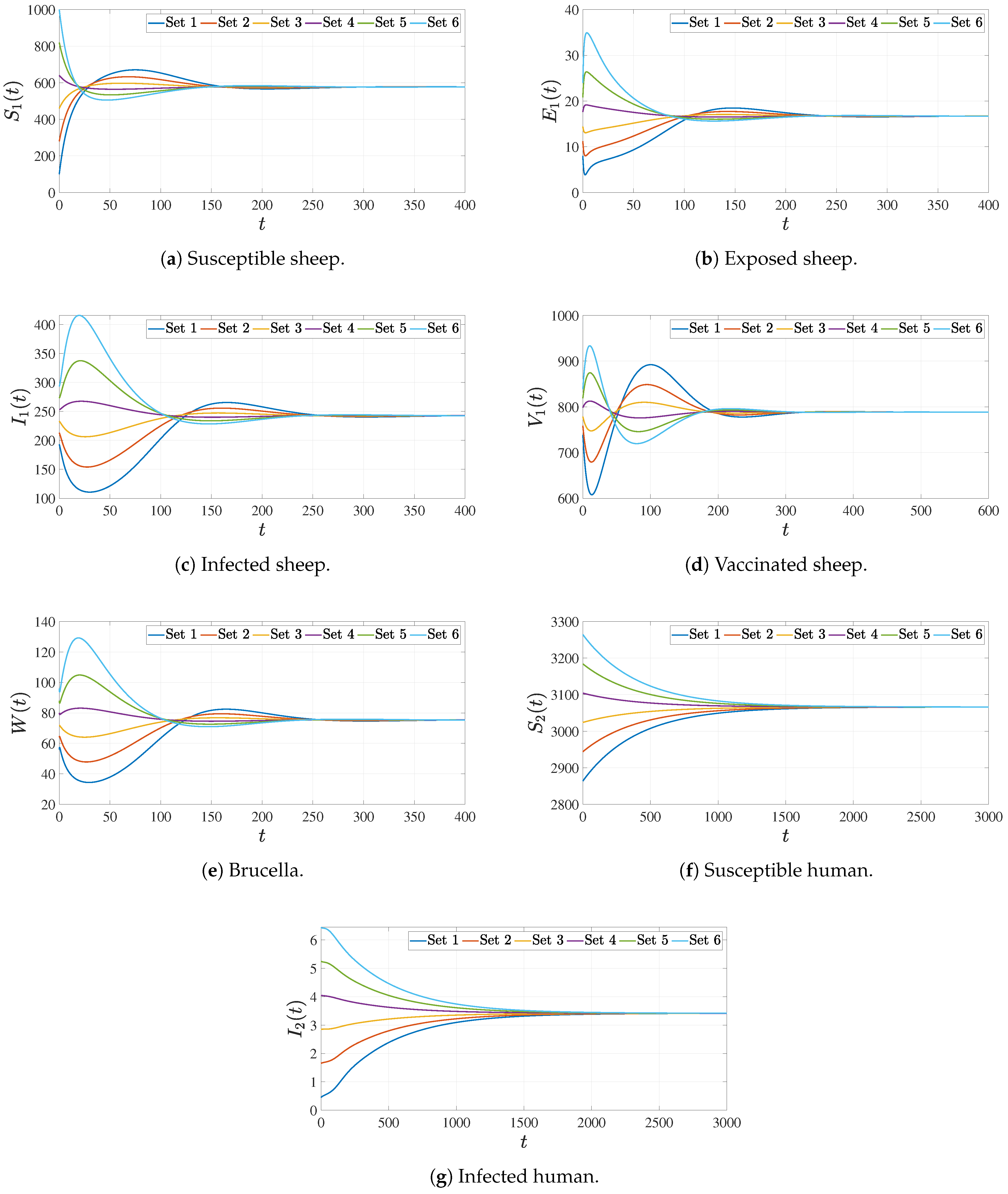
The discretized delay differential system (35) was numerically integrated using the RK(2,3) method. All computational simulations were implemented in MATLAB R2022b, relying on custom scripts that invoked the built-in DDE solver dde23, which is based on an explicit Runge–Kutta (2,3) pair with interpolation for delayed arguments. Note that MATLAB’s dde23 internally uses adaptive step-size control even when the output mesh is sampled uniformly [34]. Initial history functions were prescribed as constant values over the interval $[-\omega ,0]$, in accordance with the conditions specified in (3) and (4) using the parameter values provided in Table 3 and initial history values listed in Table 4 and Table 5.

Table 4. Sets of constant history values of ($S_1\left(\theta \right),E_1\left(\theta \right),I_1\left(\theta \right),V_1\left(\theta \right),W\left(\theta \right),S_2\left(\theta \right),I_2\left(\theta \right)$) for $\theta \in [-\omega ,0]=[-0.1,0]$ used for Figure 2.

Variable	Set 1	Set 2	Set 3	Set 4	Set 5	Set 6
$S_1\left(\theta \right)$	100	280	460	640	820	1000
$E_1\left(\theta \right)$	10	28	46	64	82	100
$I_1\left(\theta \right)$	50	90	130	170	210	250
$V_1\left(\theta \right)$	100	320	540	760	980	1200
$W\left(\theta \right)$	10	30	50	70	90	110
$S_2\left(\theta \right)$	50	88	126	164	202	240
$I_2\left(\theta \right)$	10	26	42	58	74	90

Table 4. Sets of constant history values of ($S_1\left(\theta \right),E_1\left(\theta \right),I_1\left(\theta \right),V_1\left(\theta \right),W\left(\theta \right),S_2\left(\theta \right),I_2\left(\theta \right)$) for $\theta \in [-\omega ,0]=[-0.1,0]$ used for Figure 2.

Variable	Set 1	Set 2	Set 3	Set 4	Set 5	Set 6
$S_1\left(\theta \right)$	100	280	460	640	820	1000
$E_1\left(\theta \right)$	10	28	46	64	82	100
$I_1\left(\theta \right)$	50	90	130	170	210	250
$V_1\left(\theta \right)$	100	320	540	760	980	1200
$W\left(\theta \right)$	10	30	50	70	90	110
$S_2\left(\theta \right)$	50	88	126	164	202	240
$I_2\left(\theta \right)$	10	26	42	58	74	90

Table 5. Sets of constant history values of ($S_1\left(\theta \right),E_1\left(\theta \right),I_1\left(\theta \right),V_1\left(\theta \right),W\left(\theta \right),S_2\left(\theta \right),I_2\left(\theta \right)$) for $\theta \in [-\omega ,0]=[-0.1,0]$ used for Figure 3.

Variable	Set 1	Set 2	Set 3	Set 4	Set 5	Set 6
$S_1\left(\theta \right)$	100	280	460	640	820	1000
$E_1\left(\theta \right)$	8	11.2	14.4	17.6	20.8	24
$I_1\left(\theta \right)$	193	213	233	253	273	293
$V_1\left(\theta \right)$	738.6	758.6	778.6	798.6	818.6	838.6
$W\left(\theta \right)$	56	64	72	8	88	96
$S_2\left(\theta \right)$	2864	2944	3024	3104	3184	3264
$I_2\left(\theta \right)$	0.45	1.65	2.85	4.05	5.25	6.45

Table 5. Sets of constant history values of ($S_1\left(\theta \right),E_1\left(\theta \right),I_1\left(\theta \right),V_1\left(\theta \right),W\left(\theta \right),S_2\left(\theta \right),I_2\left(\theta \right)$) for $\theta \in [-\omega ,0]=[-0.1,0]$ used for Figure 3.

Variable	Set 1	Set 2	Set 3	Set 4	Set 5	Set 6
$S_1\left(\theta \right)$	100	280	460	640	820	1000
$E_1\left(\theta \right)$	8	11.2	14.4	17.6	20.8	24
$I_1\left(\theta \right)$	193	213	233	253	273	293
$V_1\left(\theta \right)$	738.6	758.6	778.6	798.6	818.6	838.6
$W\left(\theta \right)$	56	64	72	8	88	96
$S_2\left(\theta \right)$	2864	2944	3024	3104	3184	3264
$I_2\left(\theta \right)$	0.45	1.65	2.85	4.05	5.25	6.45

Figure 2. Dynamics of Brucella Disease with ${\mathcal{R}}_0\approx 0.02<1$. Each color corresponds to one set of initial history values listed in Table 4.

Figure 2. Dynamics of Brucella Disease with ${\mathcal{R}}_0\approx 0.02<1$. Each color corresponds to one set of initial history values listed in Table 4.

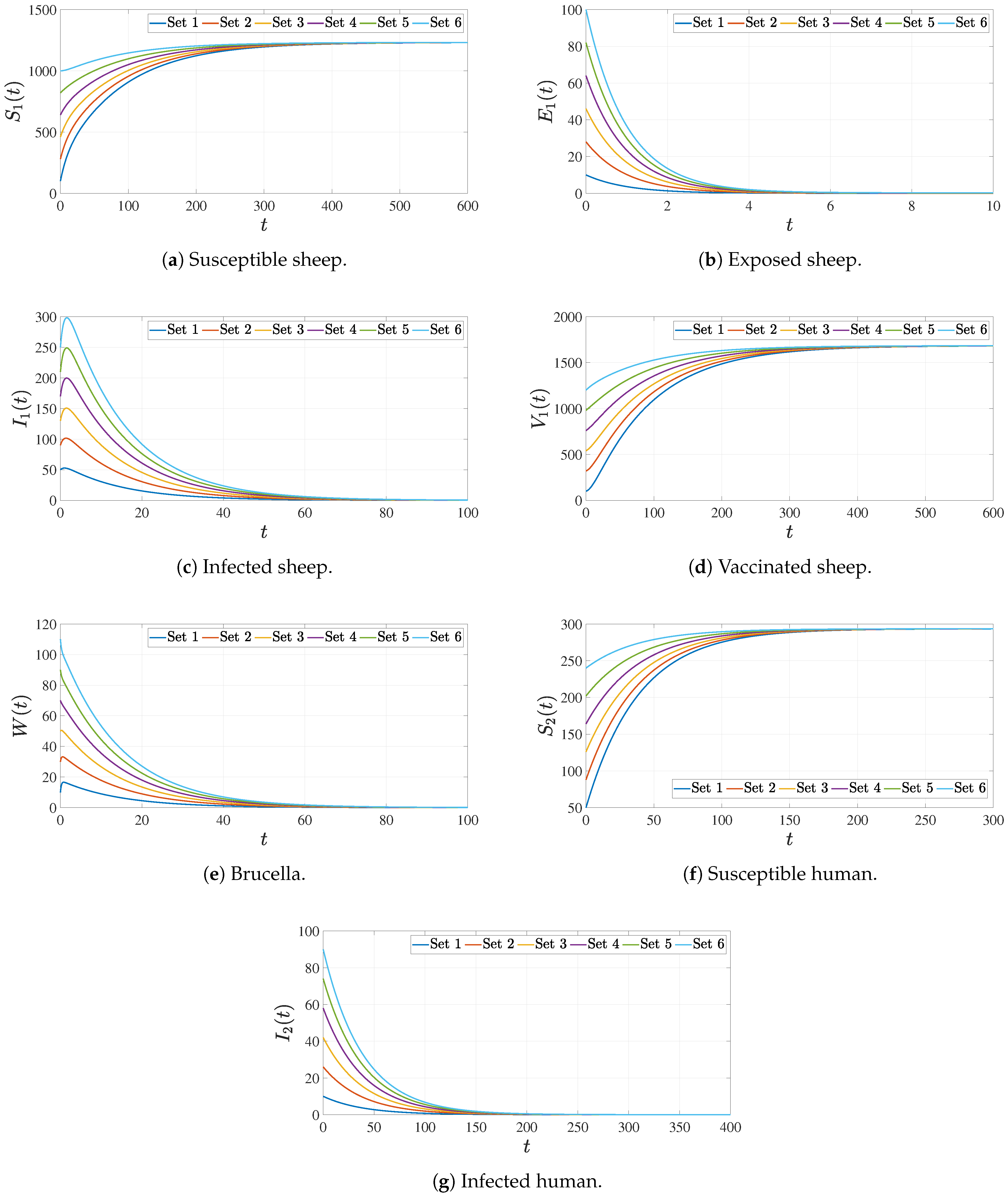
Figure 3. Dynamics of Brucella Disease with ${\mathcal{R}}_0\approx 2.14>1$. Each color corresponds to one set of initial history values listed in Table 5.

Figure 3. Dynamics of Brucella Disease with ${\mathcal{R}}_0\approx 2.14>1$. Each color corresponds to one set of initial history values listed in Table 5.

4.1. Numerical Verification of Global Asymptotic Stability

To validate the theoretical stability results established in Section 3, we now present numerical simulations that illustrate the global dynamical behavior of the brucellosis transmission model under different epidemiological scenarios. Using the parameter sets provided in Table 3, we compute the basic reproduction number ${\mathcal{R}}_0$ and examine the long-term evolution of all state variables for multiple initial conditions. Specifically, we demonstrate that when ${\mathcal{R}}_0<1$, the disease-free equilibrium is globally asymptotically stable, leading to disease eradication regardless of the initial outbreak magnitude. Conversely, when ${\mathcal{R}}_0>1$, the endemic equilibrium is globally asymptotically stable, indicating persistent brucellosis circulation within both sheep and human populations. These numerical experiments corroborate the Lyapunov functional arguments and LaSalle’s invariance principle employed in Theorems 2 and 3.

Figure 2 and Figure 3 illustrate the global asymptotic stability of the disease-free and endemic equilibrium points, respectively, under different regimes of the basic reproduction number ${\mathcal{R}}_0$. In Figure 2, with ${\mathcal{R}}_0\approx 0.02<1$, all state variables—including susceptible and vaccinated sheep ($S_1$, $V_1$), exposed and infectious sheep ($E_1$, $I_1$), environmental brucella load (W), and susceptible and infected humans ($S_2$, $I_2$)—converge to the disease-free equilibrium ${\mathcal{E}}_0$ regardless of initial conditions. Biologically, this indicates that brucellosis cannot sustain transmission and naturally dies out from both host populations and the environment. Mathematically, this confirms Theorem 2, where the Lyapunov functional ${\mathcal{F}}_1$ ensures ${\dot{\mathcal{F}}}_1\le 0$ with equality only at ${\mathcal{E}}_0$. In contrast, Figure 3 (not explicitly shown in the excerpt but implied in the numerical simulation section for ${\mathcal{R}}_0>1$) demonstrates the global attraction to the unique endemic equilibrium ${\mathcal{E}}^{*}$, where the disease persists endemically. Each compartment stabilizes at a positive steady state, reflecting sustained transmission dynamics. The convergence from multiple initial trajectories visually supports Theorem 3, illustrating that the Lyapunov-based construction ${\mathcal{F}}_3$ and ${\mathcal{F}}_4$ successfully capture the nonlinear feedback mechanisms driving the system toward ${\mathcal{E}}^{*}$. Together, these figures provide strong numerical validation of the threshold dynamics governed by ${\mathcal{R}}_0$.

4.2. Parameter Sensitivity and Determinants of ${\mathcal{R}}_0$

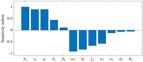
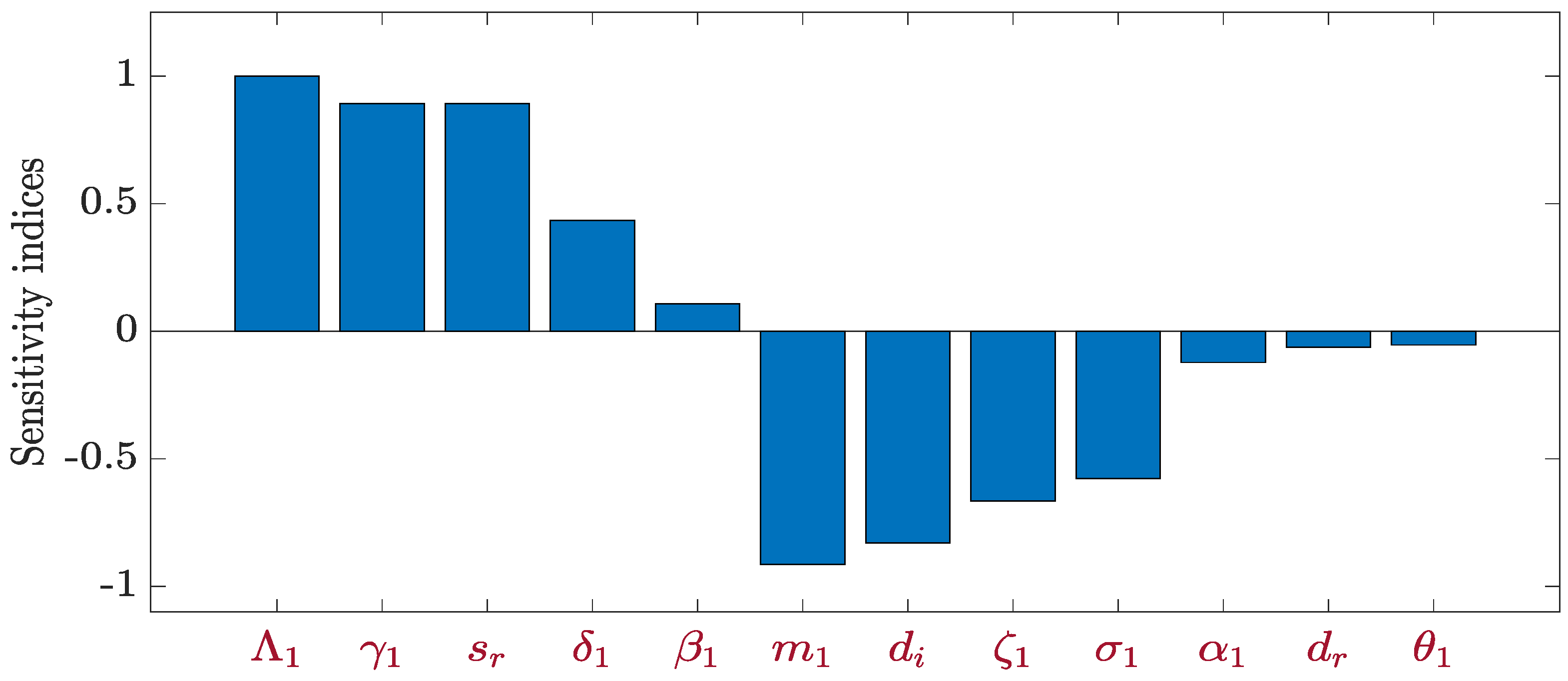
Understanding how variations in model parameters influence the basic reproduction number ${\mathcal{R}}_0$ is crucial for identifying effective control strategies. In this subsection, we perform a sensitivity analysis of ${\mathcal{R}}_0$ with respect to each epidemiological parameter using the normalized forward sensitivity index method (see Equations (39)–(50)). This approach quantifies the relative impact of parameters such as transmission rates, vaccination coverage, mortality rates, and environmental decay on disease persistence. The computed sensitivity indices, summarized in Table 6 and visualized in Figure 4, reveal which parameters, when increased, promote or suppress brucellosis transmission. Positive indices indicate that raising the corresponding parameter elevates ${\mathcal{R}}_0$, thereby increasing disease burden, while negative indices suggest a mitigating effect. Such analysis provides quantitative guidance for public health interventions, highlighting the most influential targets for reducing ${\mathcal{R}}_0$ below the critical threshold of unity.

Table 6. Sensitivity indices of ${\mathcal{R}}_0$.

Parameter	Index Expression	Value
${\Lambda }_1$	1	1
${\gamma }_1$	${\displaystyle \frac{{\displaystyle \frac{{\gamma }_1{s}_r}{d_r+d_i}}}{{\beta }_1+{\displaystyle \frac{{\gamma }_1{s}_r}{d_r+d_i}}}}$	$0.8925$
$s_r$	${\displaystyle \frac{{\displaystyle \frac{{\gamma }_1{s}_r}{d_r+d_i}}}{{\beta }_1+{\displaystyle \frac{{\gamma }_1{s}_r}{d_r+d_i}}}}$	$0.8925$
${\delta }_1$	${\displaystyle \frac{{\delta }_1}{{\delta }_1+m_1}}-{\displaystyle \frac{{\delta }_1}{{\delta }_1+{\sigma }_1+m_1}}$	$0.4341$
${\beta }_1$	${\displaystyle \frac{{\beta }_1}{{\beta }_1+{\displaystyle \frac{{\gamma }_1{s}_r}{d_r+d_i}}}}$	$0.1075$
$m_1$	${\displaystyle \frac{m_1}{{\theta }_1+{\alpha }_1+{\zeta }_1+m_1}}-{\displaystyle \frac{{\delta }_1}{{\delta }_1+m_1}}-{\displaystyle \frac{m_1}{{\theta }_1+m_1}}-{\displaystyle \frac{m_1}{{\delta }_1+{\sigma }_1+m_1}}-{\displaystyle \frac{m_1}{{\alpha }_1+{\zeta }_1+m_1}}$	$-0.9139$
$d_i$	$-{\displaystyle \frac{{\displaystyle \frac{{\gamma }_1{s}_r}{d_r+d_i}}}{{\beta }_1+{\displaystyle \frac{{\gamma }_1{s}_r}{d_r+d_i}}}}·{\displaystyle \frac{d_i}{d_r+d_i}}$	$-0.8303$
${\zeta }_1$	${\displaystyle \frac{{\zeta }_1}{{\theta }_1+{\alpha }_1+{\zeta }_1+m_1}}-{\displaystyle \frac{{\zeta }_1}{{\alpha }_1+{\zeta }_1+m_1}}$	$-0.6653$
${\sigma }_1$	$-{\displaystyle \frac{{\sigma }_1}{{\delta }_1+{\sigma }_1+m_1}}$	$-0.5775$
${\alpha }_1$	${\displaystyle \frac{{\alpha }_1}{{\theta }_1+{\alpha }_1+{\zeta }_1+m_1}}-{\displaystyle \frac{{\alpha }_1}{{\alpha }_1+{\zeta }_1+m_1}}$	$-0.1222$
$d_r$	$-{\displaystyle \frac{{\displaystyle \frac{{\gamma }_1{s}_r}{d_r+d_i}}}{{\beta }_1+{\displaystyle \frac{{\gamma }_1{s}_r}{d_r+d_i}}}}·{\displaystyle \frac{d_r}{d_r+d_i}}$	$-0.0623$
${\theta }_1$	${\displaystyle \frac{{\theta }_1}{{\theta }_1+{\alpha }_1+{\zeta }_1+m_1}}-{\displaystyle \frac{{\theta }_1}{{\theta }_1+m_1}}$	$-0.0537$

Figure 4. Sensitivity analysis of ${\mathcal{R}}_0$: relative impact of model parameters on brucellosis transmission.

The normalized forward sensitivity index of ${\mathcal{R}}_0$ with respect to a parameter q is

$${{\rm Y}}_q^{{\mathcal{R}}_0}={\displaystyle \frac{\partial {\mathcal{R}}_0}{\partial q}}·{\displaystyle \frac{q}{{\mathcal{R}}_0}}.$$

(37)

In our case, the basic reproduction number ${\mathcal{R}}_0$ is given by

$${\mathcal{R}}_0={\displaystyle \frac{{\Lambda }_1({\delta }_1+m_1)({\theta }_1+{\alpha }_1+{\zeta }_1+m_1)}{m_1({\theta }_1+m_1)({\delta }_1+{\sigma }_1+m_1)({\alpha }_1+{\zeta }_1+m_1)}}\left({\beta }_1+{\displaystyle \frac{{\gamma }_1{s}_r}{d_r+d_i}}\right).$$

(38)

4.3. Sensitivity Indices

• Recruitment rate ${\Lambda }_1$:

$${{\rm Y}}_{{\Lambda }_1}^{{\mathcal{R}}_0}=1.$$

(39)

• Transmission rate ${\beta }_1$:

$${{\rm Y}}_{{\beta }_1}^{{\mathcal{R}}_0}={\displaystyle \frac{{\beta }_1}{{\beta }_1+{\displaystyle \frac{{\gamma }_1{s}_r}{d_r+d_i}}}}.$$

(40)

• Indirect transmission rate ${\gamma }_1$:

$${{\rm Y}}_{{\gamma }_1}^{{\mathcal{R}}_0}={\displaystyle \frac{{\displaystyle \frac{{\gamma }_1{s}_r}{d_r+d_i}}}{{\beta }_1+{\displaystyle \frac{{\gamma }_1{s}_r}{d_r+d_i}}}}.$$

(41)

• Shedding rate $s_r$:

$${{\rm Y}}_{s_r}^{{\mathcal{R}}_0}={\displaystyle \frac{{\displaystyle \frac{{\gamma }_1{s}_r}{d_r+d_i}}}{{\beta }_1+{\displaystyle \frac{{\gamma }_1{s}_r}{d_r+d_i}}}}.$$

(42)

• Decay rate $d_r$:

$${{\rm Y}}_{d_r}^{{\mathcal{R}}_0}=-{\displaystyle \frac{{\displaystyle \frac{{\gamma }_1{s}_r}{d_r+d_i}}}{{\beta }_1+{\displaystyle \frac{{\gamma }_1{s}_r}{d_r+d_i}}}}·{\displaystyle \frac{d_r}{d_r+d_i}}.$$

(43)

• Disinfection rate $d_i$:

$${{\rm Y}}_{d_i}^{{\mathcal{R}}_0}=-{\displaystyle \frac{{\displaystyle \frac{{\gamma }_1{s}_r}{d_r+d_i}}}{{\beta }_1+{\displaystyle \frac{{\gamma }_1{s}_r}{d_r+d_i}}}}·{\displaystyle \frac{d_i}{d_r+d_i}}.$$

(44)

• Natural death rate $m_1$:

$${{\rm Y}}_{m_1}^{{\mathcal{R}}_0}={\displaystyle \frac{m_1}{{\delta }_1+m_1}}+{\displaystyle \frac{m_1}{{\theta }_1+{\alpha }_1+{\zeta }_1+m_1}}-1-{\displaystyle \frac{m_1}{{\theta }_1+m_1}}-{\displaystyle \frac{m_1}{{\delta }_1+{\sigma }_1+m_1}}-{\displaystyle \frac{m_1}{{\alpha }_1+{\zeta }_1+m_1}}.$$

(45)

• Vaccination rate ${\sigma }_1$:

$${{\rm Y}}_{{\sigma }_1}^{{\mathcal{R}}_0}=-{\displaystyle \frac{{\sigma }_1}{{\delta }_1+{\sigma }_1+m_1}}.$$

(46)

• Loss of immunity ${\delta }_1$:

$${{\rm Y}}_{{\delta }_1}^{{\mathcal{R}}_0}={\displaystyle \frac{{\delta }_1}{{\delta }_1+m_1}}-{\displaystyle \frac{{\delta }_1}{{\delta }_1+{\sigma }_1+m_1}}.$$

(47)

• Incubation rate ${\theta }_1$:

$${{\rm Y}}_{{\theta }_1}^{{\mathcal{R}}_0}={\displaystyle \frac{{\theta }_1}{{\theta }_1+{\alpha }_1+{\zeta }_1+m_1}}-{\displaystyle \frac{{\theta }_1}{{\theta }_1+m_1}}.$$

(48)

• Disease-induced death rate ${\alpha }_1$:

$${{\rm Y}}_{{\alpha }_1}^{{\mathcal{R}}_0}={\displaystyle \frac{{\alpha }_1}{{\theta }_1+{\alpha }_1+{\zeta }_1+m_1}}-{\displaystyle \frac{{\alpha }_1}{{\alpha }_1+{\zeta }_1+m_1}}.$$

(49)

• Culling rate ${\zeta }_1$:

$${{\rm Y}}_{{\zeta }_1}^{{\mathcal{R}}_0}={\displaystyle \frac{{\zeta }_1}{{\theta }_1+{\alpha }_1+{\zeta }_1+m_1}}-{\displaystyle \frac{{\zeta }_1}{{\alpha }_1+{\zeta }_1+m_1}}.$$

(50)

4.4. Interpretation

• Positive indices indicate that increasing the parameter increases ${\mathcal{R}}_0$.
• Negative indices indicate that increasing the parameter decreases ${\mathcal{R}}_0$.
• Parameters ${\beta }_1$, ${\gamma }_1$, and $s_r$ positively influence disease transmission.
• Control parameters such as ${\sigma }_1$, $d_r$, and $d_i$ reduce ${\mathcal{R}}_0$.

The expressions of sensitivity indices and their values are given in Table 6 for the parameters values given in Table 3.

Table 6 and Figure 4 present the normalized forward sensitivity indices of the basic reproduction number ${\mathcal{R}}_0$ with respect to the key parameters of the brucellosis model, offering both biological insight and mathematical guidance for disease control. Mathematically, a positive index indicates that an increase in the corresponding parameter leads to an increase in ${\mathcal{R}}_0$, thereby promoting disease persistence, while a negative index implies that increasing the parameter reduces ${\mathcal{R}}_0$ and supports disease eradication. Biologically, the recruitment rate ${\Lambda }_1$ exhibits the highest positive sensitivity (index = 1), meaning that any proportional increase in sheep birth or importation directly scales ${\mathcal{R}}_0$ linearly, highlighting the importance of population management. The indirect transmission pathway via the environment dominates the dynamics, as reflected by the high sensitivity indices of ${\gamma }_1$ and $s_r$ (both approximately 0.8925), indicating that reducing environmental contamination or shedding rates would substantially lower ${\mathcal{R}}_0$. In contrast, the disinfection rate $d_i$ (index = $-0.8303$) and culling rate ${\zeta }_1$ (index = $-0.6653$) show strong negative sensitivities, making them potent intervention levers. Surprisingly, the natural mortality rate $m_1$ exhibits a large negative index ($-0.9139$), which is mathematically expected when disease-induced death is low but biologically implies that increasing sheep mortality is neither ethical nor practical as a control strategy. The vaccination rate ${\sigma }_1$ (index = $-0.5775$) and the loss of immunity rate ${\delta }_1$ (positive index = 0.4341) further underscore the dual role of vaccination: enhancing vaccination coverage reduces ${\mathcal{R}}_0$, whereas waning immunity restores susceptibility and elevates transmission risk. Together, these sensitivity results quantitatively prioritize interventions: environmental disinfection, sheep culling, and vaccination offer the greatest potential for reducing ${\mathcal{R}}_0$ below unity, while direct transmission ${\beta }_1$ (index = 0.1075) plays a comparatively minor role.

Furthermore, we have:

• For every 10% increase in the disinfection rate $d_i$, ${\mathcal{R}}_0$ decreases by approximately 8.3%, making environmental sanitation a highly efficient intervention. In contrast, a 10% increase in direct transmission ${\beta }_1$ raises ${\mathcal{R}}_0$ by only 1.1%, indicating that controlling indirect pathways is more impactful.
• The culling (${\zeta }_1$) has a negative index $-0.665$, but its ethical and economic costs must be weighed against disinfection which is similarly effective. Vaccination (${\sigma }_1$) is moderately effective (−0.577) and likely more socially acceptable.

4.5. Evaluating Treatment Efficacy for Outbreak Mitigation

Having identified through sensitivity analysis the parameters that most strongly influence ${\mathcal{R}}_0$, we now investigate the potential of treatment interventions as a practical control strategy. In this subsection, we introduce a treatment efficacy parameter $p\in [0,1]$ that reduces the effective transmission rates of brucellosis within the sheep population, as shown in model system (51). The modified basic reproduction number ${\mathcal{R}}_0^{\mathrm{treatment}}\left(p\right)=(1-p){\mathcal{R}}_0$ quantifies the combined effect of treatment on both direct and indirect transmission pathways. By analyzing the critical treatment efficacy $p^{\mathrm{cr}}=1-1/{\mathcal{R}}_0$, we determine the minimum level of intervention required to drive ${\mathcal{R}}_0^{\mathrm{treatment}}$ below unity, thereby ensuring global asymptotic stability of the disease-free equilibrium. Numerical simulations illustrate the transition from endemic persistence to disease eradication as p increases beyond this threshold, providing practical guidance for resource allocation in brucellosis control programs.

Model (51) represents the same biological system as (1)–(2) but with the introduction of an intervention: treatment efficacy p reduces both direct transmission (${\beta }_1$) and indirect transmission (${\gamma }_1$) by a factor $(1-p)$. This models a combined treatment (e.g., antibiotics in sheep, vaccination with high efficacy, or biocontrol) that reduces infectiousness/susceptibility.

The parameter p encapsulates the net effect of public health interventions (mass treatment, vaccination coverage, or improved farm biosecurity) that proportionally lower the effective contact rates, independent of the transmission route.

By adding a treatment efficacy parameter $p\in [0,1]$, the mathematical model (1)–(2) takes the following form:

$$\begin{array}{c}\hfill \left\{\begin{array}{ccc}{\displaystyle \frac{\mathrm{d}{S}_1}{\mathrm{d}t}}\hfill & =\hfill & {\Lambda }_1-(1-p){\beta }_1{S}_1(E_1+I_1)-(1-p){\gamma }_1{S}_{1}W+{\delta }_1{V}_1-({\sigma }_1+m_1)S_1,\hfill \\ {\displaystyle \frac{\mathrm{d}{E}_1}{\mathrm{d}t}}\hfill & =\hfill & (1-p){\beta }_1{S}_1(E_1+I_1)+(1-p){\gamma }_1{S}_{1}W-({\theta }_1+m_1)E_1,\hfill \\ {\displaystyle \frac{\mathrm{d}{I}_1}{\mathrm{d}t}}\hfill & =\hfill & {\theta }_1{E}_1-({\alpha }_1+{\zeta }_1+m_1)I_1,\hfill \\ {\displaystyle \frac{\mathrm{d}{V}_1}{\mathrm{d}t}}\hfill & =\hfill & {\sigma }_1{S}_1-({\delta }_1+m_1)V_1,\hfill \\ {\displaystyle \frac{\mathrm{d}W}{\mathrm{d}t}}\hfill & =\hfill & s_r(E_1+I_1)-(d_r+d_i)W,\hfill \\ {\displaystyle \frac{\mathrm{d}{S}_2}{\mathrm{d}t}}\hfill & =\hfill & {\Lambda }_2-{\beta }_2{S}_2((1+m_1)E_1+(1+{\alpha }_1+m_1)I_1)-{\gamma }_2{S}_{2}W-m_2{S}_2,\hfill \\ {\displaystyle \frac{\mathrm{d}{I}_2}{\mathrm{d}t}}\hfill & =\hfill & {\beta }_2{e}^{-n\tau }{S}_2^{\tau }\left((1+m_1)E_1^{\tau }+(1+{\alpha }_1+m_1)I_1^{\tau }\right)+{\gamma }_2{e}^{-n\tau }{S}_2^{\tau }{W}^{\tau }-m_2{I}_2.\hfill \end{array}\right.\end{array}$$

(51)

According to the reproductive number ${\mathcal{R}}_0$ discussed previously, the basic reproductive number for model (51) is given by ${\mathcal{R}}_0^{\mathrm{treatment}}\left(p\right)=(1-p){\mathcal{R}}_0\le {\mathcal{R}}_0$. Assume that ${\mathcal{R}}_0>1$, and we aim to impose ${\mathcal{R}}_0^{\mathrm{treatment}}\left(p\right)\le 1$ which imply the stability of ${\mathcal{E}}_0$. The critical value of the treatment efficacy $p^{\mathrm{cr}}$ is given by:

$$\begin{array}{c}\hfill \begin{array}{cc}{\mathcal{R}}_0^{\mathrm{treatment}}\left(p^{\mathrm{cr}}\right)\hfill & =1⟹p^{\mathrm{cr}}=1-{\displaystyle \frac{1}{{\mathcal{R}}_0}}.\hfill \end{array}\end{array}$$

(52)

Then we get ${\mathcal{R}}_0^{\mathrm{treatment}}\left(p\right)\le 1\mathrm{for}\mathrm{all}{p}^{\mathrm{cr}}\le p\le 1$, and thus ${\mathcal{E}}_0$ is GAS. By choosing ${\beta }_1=1.12\times {10}^{-4}$, we get $p^{\mathrm{cr}}\approx 0.5317$. Therefore,

(i)

if $0.5317\le p\le 1$, then ${\mathcal{R}}_0^{\mathrm{treatment}}\left(p\right)\le 1$, and ${\mathcal{E}}_0$ is GAS;

(ii)

if $0\le p<0.5317$, then ${\mathcal{R}}_0^{\mathrm{treatment}}\left(p\right)>1$, and ${\mathcal{E}}_0$ becomes unstable, and ${\mathcal{E}}^{*}$ becomes GAS.

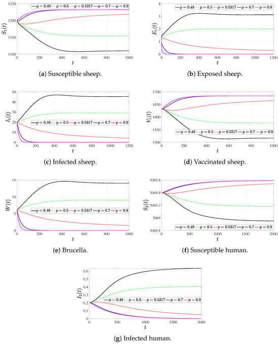
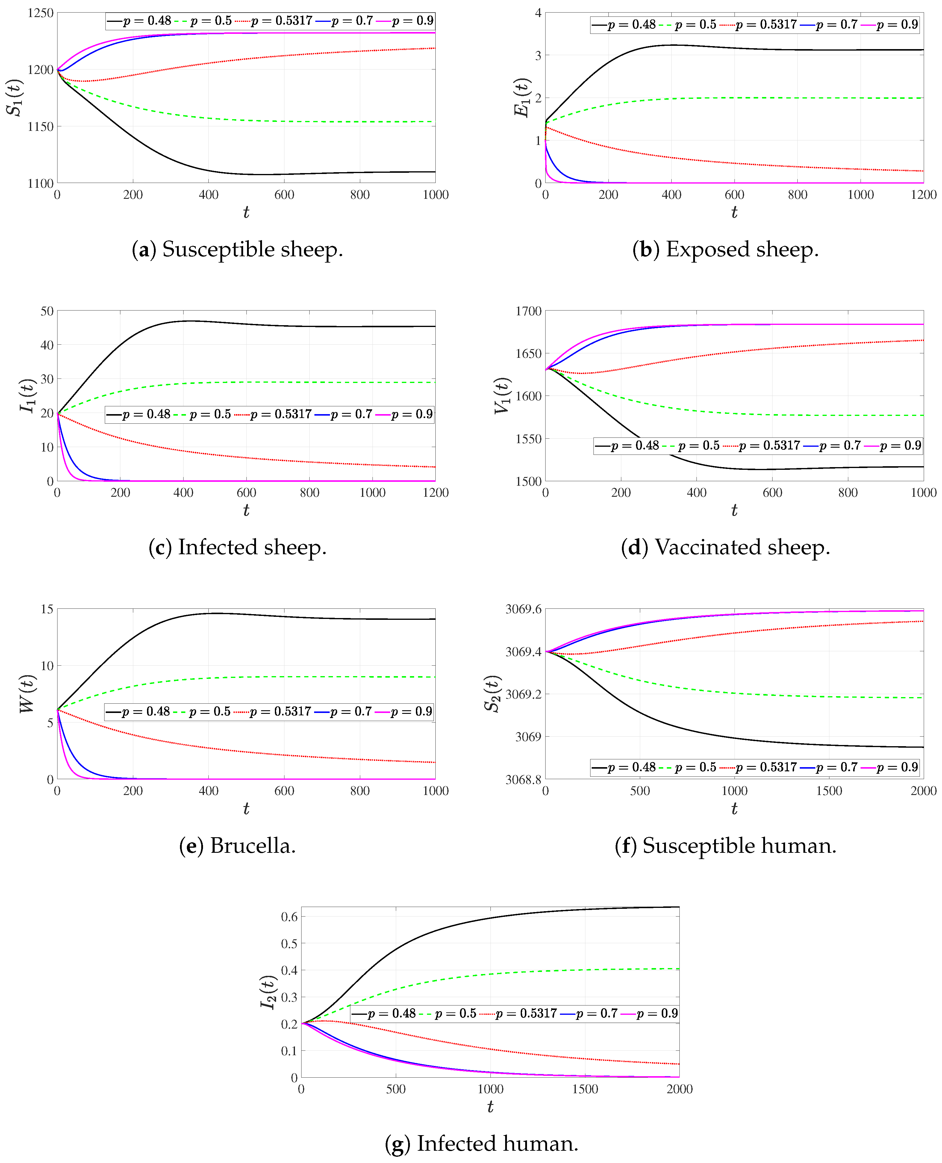
Table 7 and Figure 5 collectively elucidate the threshold behavior of brucellosis transmission under varying treatment efficacy p, bridging mathematical theory with practical disease management. Mathematically, Table 7 demonstrates the linear relationship $R_0^{\mathrm{treatment}}\left(p\right)=(1-p)R_0$, where increasing treatment efficacy proportionally reduces the basic reproduction number. The critical threshold $p^{\mathrm{cr}}=1-1/R_0\approx 0.5317$ represents a transcritical bifurcation point: for $p<p^{\mathrm{cr}}$, we have $R_0^{\mathrm{treatment}}>1$ and the endemic equilibrium remains globally asymptotically stable; for $p\ge p^{\mathrm{cr}}$, we obtain $R_0^{\mathrm{treatment}}\le 1$ and the disease-free equilibrium becomes globally asymptotically stable. Biologically, this means that treatment must achieve at least approximately 53.2% efficacy in reducing transmission to guarantee disease eradication, assuming the baseline $R_0\approx 2.136$ (since $p^{\mathrm{cr}}=1-1/2.136\approx 0.5317$). Figure 5 visually confirms this analytical prediction through time-series simulations under different p values. When $p=0$ (no treatment), infected populations persist at high endemic levels. As p increases to 0.3 and 0.5, although infection peaks are reduced, the disease continues to circulate endemically. Only when p reaches or exceeds the critical value $0.5317$ do all infected compartments (sheep $I_1$, humans $I_2$, and environmental brucella W) converge monotonically to zero, while susceptible populations stabilize at their disease-free equilibrium levels. This threshold behavior highlights that suboptimal treatment efforts, while beneficial, are insufficient for eradication and may lead to persistent low-level transmission. From a public health perspective, these results provide a quantifiable target: interventions designed to reduce sheep-to-sheep and environment-to-sheep transmission by more than 53% can achieve local elimination of brucellosis, whereas weaker interventions only mitigate but do not eliminate the disease burden.

Table 7. Relationship between treatment efficacy p and ${\mathcal{R}}_0^{\mathrm{treatment}}\left(p\right)$. Values below the critical threshold $p^{\mathrm{cr}}$ maintain disease persistence, while higher values lead to eradication.

p	$0.48$	$0.5$	$0.5317$	$0.7$	$0.9$
${\mathcal{R}}_0^{\mathrm{treatment}}\left(p\right)$	$1.1103$	$1.0676$	1	$0.6406$	$0.2135$

Figure 5. Time series of all compartments under increasing treatment efficacy p. Disease eradication is achieved only when $p\ge p^{\mathrm{cr}}=1-1/{\mathcal{R}}_0$, while subthreshold treatment reduces but does not eliminate endemic circulation. The initial values are given by ($1200,1,20,1630,6,3069.4,0.2$).

4.6. Influence of Delay on Human Infection Dynamics

In the formulation of model (2), a distributed time delay $\omega$ was incorporated to account for the incubation period and the delayed effects of environmental exposure on human infection. In this subsection, we investigate the impact of this time delay on the transmission dynamics of brucellosis within the human population. By selecting the Dirac delta function as a specific probability distribution, we reduce the distributed delay model to a discrete delay system, where the parameter $\tau$ explicitly represents the average time lag between exposure and the onset of infectiousness. Numerical simulations are performed to explore how variations in $\tau$ affect the peak size, timing, and eventual persistence of human infections $I_2\left(t\right)$. Understanding the role of such delays is crucial for accurate outbreak forecasting and the design of timely intervention strategies, as delays can substantially alter the transient dynamics and the effectiveness of control measures.

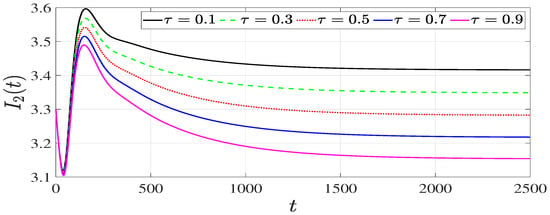
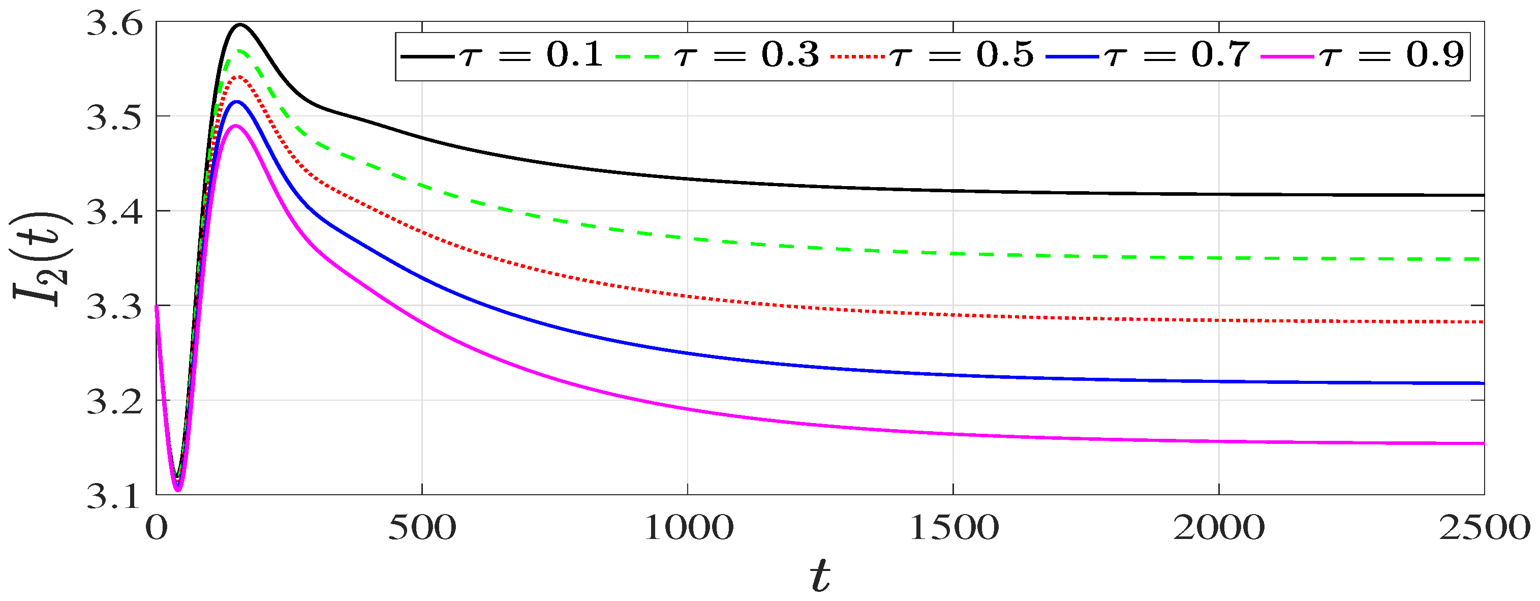
Figure 6 illustrates the effect of varying the discrete time delay $\tau$ on the dynamics of infected humans $I_2\left(t\right)$ under fixed initial conditions, providing crucial insight into how incubation periods and environmental exposure lags shape brucellosis outbreaks. Mathematically, the delay enters the human infection terms through the factor $e^{-n\tau }$ (where n is a constant related to the probability distribution) and through the delayed state variables $S_2(t-\tau )$, $E_1(t-\tau )$, $I_1(t-\tau )$, and $W(t-\tau )$ in system (35). As $\tau$ increases from small to larger values, several key dynamical features emerge: the peak of the infected human population is progressively delayed in time, corresponding to a longer interval between exposure and the manifestation of infectiousness or between environmental contamination and human contact. Additionally, the magnitude of the infection peak may decrease with increasing $\tau$, suggesting that longer incubation or delayed exposure pathways can dampen the acute phase of an outbreak. Biologically, this delay represents the combined effects of (i) the incubation period of brucellosis in humans before symptoms appear, (ii) the time lag between brucella shedding by infected sheep and subsequent human exposure, and (iii) the interval between exposure and effective transmission. In real-world settings, longer delays allow more time for public health interventions—such as case isolation, environmental disinfection, or public awareness campaigns—to be implemented before the infection burden peaks. However, the figure also shows that regardless of $\tau$, all trajectories eventually converge to the same steady state (either disease-free or endemic, depending on ${\mathcal{R}}_0$), confirming that time delays influence transient dynamics but do not alter the asymptotic stability properties predicted by ${\mathcal{R}}_0$ in this model formulation. This underscores an important mathematical principle: while delays can significantly affect outbreak timing and peak severity, the threshold condition for long-term disease persistence or eradication remains governed by the basic reproduction number.

Figure 6. Infected human dynamics under varying the delay $\tau$ for the initial value $I_2\left(0\right)=3.3$.

5. Conclusions

In this paper, we developed and rigorously analyzed a cross-species epidemic model describing the transmission dynamics of brucellosis among sheep, humans, and the environmental reservoir of Brucella. The model incorporates both direct transmission pathways (sheep-to-sheep and sheep-to-human contacts) and indirect transmission via contaminated environments, as well as vaccination in sheep, culling of infectious sheep, disinfection, and distributed time delays in human infection. By establishing the non-negativity, boundedness, and positive invariance of solutions, we demonstrated that the model is mathematically well-posed and biologically meaningful.

The basic reproduction number ${\mathcal{R}}_0$ was derived using the next-generation matrix method and serves as a threshold parameter governing the global dynamics. Using Lyapunov functionals and LaSalle’s invariance principle, we proved that if ${\mathcal{R}}_0\le 1$, the disease-free equilibrium ${\mathcal{E}}_0$ is globally asymptotically stable, implying that brucellosis can be eradicated regardless of initial conditions. Conversely, if ${\mathcal{R}}_0>1$, a unique endemic equilibrium ${\mathcal{E}}^{*}$ exists and is globally asymptotically stable, indicating persistent disease circulation.

Sensitivity analysis using normalized forward indices revealed that the environmental transmission rate ${\gamma }_1$, the shedding rate $s_r$, and the sheep recruitment rate ${\Lambda }_1$ are the most influential positive contributors to ${\mathcal{R}}_0$, while disinfection ($d_i$), culling (${\zeta }_1$), and vaccination (${\sigma }_1$) exert strong negative effects. These findings prioritize environmental sanitation and targeted culling as key intervention strategies. The introduction of treatment efficacy p showed a clear threshold: when p exceeds the critical value $p^{\mathrm{cr}}=1-1/{\mathcal{R}}_0$, the disease-free equilibrium becomes globally stable, providing a quantitative target for intervention programs.

Finally, numerical simulations of the delayed human infection model demonstrated that time delays primarily affect the timing and magnitude of infection peaks without altering asymptotic stability, highlighting the importance of prompt intervention during outbreak windows. Collectively, this work provides a comprehensive mathematical framework for understanding brucellosis transmission in coupled human–animal–environment systems and offers actionable insights for public health planning and disease control in endemic regions.

Several simplifying assumptions constrain the direct applicability of our model. First, we assume unidirectional transmission from sheep and the environment to humans, neglecting potential human-to-environment shedding or human-to-sheep feedback, which may be non-negligible in high-prevalence occupational settings. Second, the treatment efficacy parameter p homogeneously reduces both direct and indirect transmission rates by the same factor $(1-p)$, an idealization that ignores route-specific or dose-dependent treatment effects. Third, the sensitivity analysis treats all parameters as independent, whereas real-world interventions (e.g., culling and vaccination) often compete for limited resources, and environmental decay correlates with disinfection practices. Fourth, the global stability proof employs an asymptotically autonomous decoupling of the human subsystem, assuming sheep dynamics equilibrate on a faster timescale than human infection—a simplification that may not hold during early outbreak transients or under simultaneous interventions. Finally, the bilinear incidence, homogeneous mixing, and exponential delay kernel, while mathematically tractable, abstract away spatial heterogeneity, population structure, and empirical incubation distributions. Future work should relax these assumptions to enhance real-world predictive fidelity.

References

- Rees, E.M.; Minter, A.; Edmunds, W.J.; Lau, C.L.; Kucharski, A.J.; Lowe, R. Transmission modelling of environmentally persistent zoonotic diseases: A systematic review. Lancet Planet. Health 2021, 5, e466–e478. [Google Scholar] [CrossRef] [Scilit] [PubMed]
- World Health Organization. Brucellosis. 2020. Available online: https://www.who.int/news-room/fact-sheets/detail/brucellosis (accessed on 25 April 2026).
- World Organisation for Animal Health. Brucellosis. 2025. Available online: https://www.woah.org/en/disease/brucellosis/ (accessed on 25 April 2026).
- Pappas, G.; Papadimitriou, P.; Akritidis, N.; Christou, L.; Tsianos, E.V. The new global map of human brucellosis. Lancet Infect. Dis. 2006, 6, 91–99. [Google Scholar] [CrossRef] [Scilit]
- Wang, L.; Li, M.; Pei, X.; Zhang, J.; Sun, G.; Jin, Z. Cost assessment of optimal control strategy for brucellosis dynamic model based on economic factors. Commun. Nonlinear Sci. Numer. Simul. 2023, 124, 107310. [Google Scholar] [CrossRef] [Scilit]
- Gong, W.; Sun, P.; Zhai, C.; Yuan, J.; Chen, Y.; Chen, Q.; Zhao, Y. Accessibility of the three-year comprehensive prevention and control of brucellosis in Ningxia: A mathematical modeling study. BMC Infect. Dis. 2023, 23, 292. [Google Scholar] [CrossRef] [Scilit]
- He, X.; Lv, T.; Liu, J.; Zhou, L.; Fan, M. Dynamical modeling and optimal control of brucellosis with mixed delays and environmental transmission. Int. J. Biomath. 2025, 18, 2550136. [Google Scholar] [CrossRef] [Scilit]
- Hou, Q.; Sun, X.; Zhang, J.; Liu, Y.; Wang, Y.; Jin, Z. Modeling the transmission dynamics of sheep brucellosis in Inner Mongolia Autonomous Region, China. Math. Biosci. 2013, 242, 51–58. [Google Scholar] [CrossRef] [Scilit]
- Hou, Q.; Sun, X.; Wang, Y.; Huang, B.; Jin, Z. Global properties of a general dynamic model for animal diseases: A case study of brucellosis and tuberculosis transmission. J. Math. Anal. Appl. 2014, 414, 424–433. [Google Scholar] [CrossRef] [Scilit]
- Liu, S.; Hu, J.; Zhao, Y.; Wang, X.; Wang, X. Prediction and control for the transmission of brucellosis in Inner Mongolia, China. Sci. Rep. 2025, 15, 3532. [Google Scholar] [CrossRef] [Scilit]
- Sun, G.; Zhang, Z. Global stability for a sheep brucellosis model with immigration. Appl. Math. Comput. 2014, 246, 336–345. [Google Scholar] [CrossRef] [Scilit]
- Zhang, Z.; Zhang, J.; Li, L.; Guo, Z.; Zhang, Z.; Sun, G. Quantifying the effectiveness of brucellosis control strategies in northern China using a mechanistic and data-driven model. Chaos Solitons Fractals 2024, 185, 115121. [Google Scholar] [CrossRef] [Scilit]
- Li, M.; Jin, Z.; Sun, G.; Zhang, J. Modeling direct and indirect disease transmission using multi-group model. J. Math. Anal. Appl. 2017, 446, 1292–1309. [Google Scholar] [CrossRef] [Scilit]
- Yang, C.; Lolika, P.O.; Mushayabasab, S.; Wang, J. Modeling the spatiotemporal variations in brucellosis transmission. Nonlinear Anal. Real World Appl. 2017, 38, 49–67. [Google Scholar] [CrossRef] [Scilit]
- Li, M.; Sun, G.; Wu, Y.; Zhang, J.; Jin, Z. Transmission dynamics of a multi-group brucellosis model with mixed cross infection in public farm. Appl. Math. Comput. 2014, 237, 582–594. [Google Scholar] [CrossRef] [Scilit]
- Li, M.; Pei, X.; Zhang, J.; Li, L. Asymptotic analysis of endemic equilibrium to a brucellosis model. Math. Biosci. Eng. 2019, 16, 5836–5850. [Google Scholar] [CrossRef] [Scilit]
- Qin, Y.; Pei, X.; Li, M.; Chai, Y. Transmission dynamics of brucellosis with patch model: Shanxi and Hebei provinces as cases. Math. Biosci. Eng. 2022, 19, 6396–6414. [Google Scholar] [CrossRef] [Scilit] [PubMed]
- Yang, J.; Xu, R.; Li, J. Threshold dynamics of an age-space structured brucellosis disease model with Neumann boundary condition. Nonlinear Anal. Real World Appl. 2019, 50, 192–217. [Google Scholar] [CrossRef] [Scilit]
- Zheng, T.; Hao, Y.; Luo, Y.; Teng, Z. Analysis of a diffusive brucellosis model with partial immunity and stage structure in heterogeneous environment. Adv. Contin. Discret. Model. 2025, 2025, 16. [Google Scholar] [CrossRef] [Scilit]
- Chen, S.; Wei, F.; Zhang, X.; Jin, H.; Zhao, Y.; Zhang, S. Dynamic modelling and analysis of human brucellosis on age heterogeneity in Jinzhou, China. Infect. Dis. Model. 2026, 11, 1158–1179. [Google Scholar] [CrossRef] [Scilit]
- El Hajji, M.; Al-Faidi, Y.A.; Alharbi, M.H. Modeling dual-colony Nosema transmission in honeybees: The role of distributed delays and antiviral treatment. AIMS Math. 2026, 11, 2645–2681. [Google Scholar] [CrossRef] [Scilit]
- Alalhareth, F.K.; Alharbi, A.A.; Alharbi, M.H.; El Hajji, M. Modeling Guinea worm disease with time delays: Threshold dynamics, treatments and sensitivity analysis in heterogeneous populations. AIMS Math. 2026, 11, 11116–11153. [Google Scholar] [CrossRef] [Scilit]
- Alharbi, M.H.; Alzahrani, A.R. Global Dynamics for a Distributed Delay SVEIR Model for Measles Transmission with Imperfect Vaccination: A Threshold Analysis. Mathematics 2026, 14, 1219. [Google Scholar] [CrossRef] [Scilit]
- Alharbi, M.H.; Alzahrani, A.R. Threshold Dynamics of Within-Host CHIKV Infection: A Delay Differential Equation Model with Persistent Infected Monocytes and Humoral Immunity. Mathematics 2026, 14, 1331. [Google Scholar] [CrossRef] [Scilit]
- Almuashi, H.H.; El Hajji, M. Global Dynamics of a Dual-Target HIV Model with Time Delays and Treatment Implications. Mathematics 2026, 14, 6. [Google Scholar] [CrossRef] [Scilit]
- Almuallem, N.A.; El Hajji, M. Global Dynamics of a Multi-Population Water Pollutant Model with Distributed Delays. Mathematics 2026, 14, 20. [Google Scholar] [CrossRef] [Scilit]
- Alalhareth, F.K.; Albishri, M.I.; Alharbi, M.H.; El Hajji, M. Impact of Latent Reservoirs, Latent Infection Delays, and Treatments on HIV Dynamics. Mathematics 2026, 14, 1675. [Google Scholar] [CrossRef] [Scilit]
- Van den Driessche, P.; Watmough, J. Reproduction Numbers and Sub-Threshold Endemic Equilibria for Compartmental Models of Disease Transmission. Math. Biosci. 2002, 180, 29–48. [Google Scholar] [CrossRef] [Scilit] [PubMed]
- Lyapunov, A.M. The general problem of the stability of motion. Int. J. Control 1992, 55, 531–534. [Google Scholar] [CrossRef] [Scilit]
- LaSalle, J.P. The Stability of Dynamical Systems; SIAM: Philadelphia, PA, USA, 1976. [Google Scholar]
- Thieme, H.R. Asymptotically autonomous differential equations in the plane. Rocky Mt. J. Math. 1994, 24, 351–380. [Google Scholar] [CrossRef] [Scilit]
- Thieme, H.R. Mathematicals in Population Biology; Princeton University Press: Princeton, NJ, USA; Oxford, UK, 2003. [Google Scholar]
- Chen, K.; Wei, F.; Zhang, X.; Jin, H.; Zhou, R.; Zuo, Y.; Fan, K. Dynamics of an SVEIR transmission model with protection awareness and two strains. Infect. Dis. Model. 2025, 10, 207–228. [Google Scholar] [CrossRef] [Scilit]
- Shampine, L.; Thompson, S. Solving DDEs in Matlab. Appl. Numer. Math. 2001, 37, 441–458. [Google Scholar] [CrossRef] [Scilit]
Disclaimer/Publisher’s Note: The statements, opinions and data contained in all publications are solely those of the individual author(s) and contributor(s) and not of MDPI and/or the editor(s). MDPI and/or the editor(s) disclaim responsibility for any injury to people or property resulting from any ideas, methods, instructions or products referred to in the content. |
© 2026 by the authors. Licensee MDPI, Basel, Switzerland. This article is an open access article distributed under the terms and conditions of the Creative Commons Attribution (CC BY) license.