Skip to Content
MathematicsMathematics
  • Article
  • Open Access

4 June 2026

23 Pages

Asymptotic Behavior of Estimators for One Change-Point Detection Based on Processes Whose Kernel Function Has Degree Greater than Two

,
and
1
Department of Mathematics and Science Computer, University of Antananarivo, Antananarivo 101, Madagascar
2
Institut de Mathématiques de Toulouse, UMR5219 Université Paul Sabatier, 31062 Toulouse Cedex 9, France
3
INSPÉ de l’Académie de Limoges, Université de Limoges, 209 Boulevard de Vanteaux, 87000 Limoges, France
4
Laboratoire Vie-Santé, UR 24 134, Faculté de Médecine, Université de Limoges, 2 Av. Martin Luther King, 87025 Limoges, France

Abstract

We study change-point estimation for absolutely continuous independent and identically distributed random variables from a nonparametric point of view. We define a sequence of processes and estimators based on U-statistics, whose kernel function has a degree greater than two. We then propose to extend the results in the literature on the asymptotic behavior of a sequence of processes and estimators, in the case of the existence or not of a change point. Numerical simulations are provided to support the theoretical results.
MSC:
60G10; 62G05

1. Introduction

The change-point problem was first considered by Page [1,2] for quality control. Since then, many authors have explored the topic. Among others, Chernoff and Zack [3] have proposed test statistics for detecting shifts in the mean of the normal distribution function. A review of parametric procedures for the change-point problem is given by Wolfe and Schechtman [4]. Csörgö and Horvath [5] have obtained invariance principles for tests based on U-statistics-type processes and Csörgö and Horvath [6] have proposed a review of twenty nonparametric methods for change-point problems.
The study of change points was developed through different aspects and different approaches. In a nonparametric framework, Döring [7] has proposed the maximizing point of weighted multivariate U-statistic process as the estimator of the change point. He has proved, under mild moment conditions, almost certain convergence and the rate of convergence. Ciuperca [8] has studied a general criterion to determine the number of change points. Mohr and Selk [9] have considered a regression model that allows for time series covariates as well as heteroscedasticity with a regression function modeled nonparametrically. They have shown the consistency of the estimator of the change-point based on a Kolmogorov–Smirnov functional of the marked empirical process of residuals and they have proved an optimal rate of convergence. For detecting epidemic changes, Rackauskas and Wendler [10] have presented a robust test statistic based on the Wilcoxon statistic and have proved a functional central limit theorem for U-processes in Hölder spaces. Ngatchou-Wandji et al. [11] have studied some change-point tests based on U-statistics for weakly dependent observations. For their part, Ngatchou-Wandji et al. [12,13] have defined weak change as a change with too small a magnitude and have proposed new likelihood-based tools for weak changes’ study in the mean of class of Conditional Heteroscedastic AutoRegressive Non-Linear (CHARN) models whose the results are applied to both change detection and location estimation. On weak changes’ study again, Aouissaoui et al. [14] have proposed tests for weak changes in the conditional mean of a class of parametric conditional heteroscedastic nonlinear models. Recently, Ngatchou-Wandji et al. [15] extended the results of Ngatchou-Wandji et al. [11] by studying multiple change points for absolutely regular observations.
In this paper, we consider absolutely continuous independent random variables X 1 , … , X n , with cumulative distribution function F i , and density f i for 1 ⩽ i ⩽ n . We introduce the kernel
ϕ : R l ⟶ R , l > 2 ,
supposed bounded, integrable, differentiable, satisfying the integrability conditions and invariant for all permutations of the set { 1 , … , l } . We study the following estimator and sequence of processes:
Z n , k ( l ) = ∑ j = 1 l − 1 ∑ 1 ⩽ i 1 < … < i j ⩽ k ∑ k + 1 ⩽ i j + 1 < … < i l ⩽ n ϕ X i 1 , … , X i j , X i j + 1 , … , X i l
and
U k ( l ) = Z n , k ( l ) − ∑ j = 1 l − 1 k j n − k l − j Θ ϕ ( l ) ( F , F ) ,
where k is the eventual change point. The estimators and the sequence of processes studied previously have been constructed with kernels of degree two, for example, in Csörgö and Horvath [5]. As for us, our contribution consists of generalizing the existing results to the associated estimators and to the sequence of processes whose degree l of the kernel is greater than two; Z n , k ( l ) defined in (1) is therefore a generalization of what has been studied so far in the literature. The kernel will be a function of l consecutive variables and we study the asymptotic behavior of the estimators and the sequence of processes with much longer memory.
With a kernel of degree l greater than two, we consider in this paper two cases: the first one where F i , i = 1 , … , n have the same law and the second one corresponds to the existence of a change point, i.e, there exists an integer n 0 < n such that F n 0 and F n 0 + 1 are different.
The paper is organized as follows. In Section 2, we define the estimators and the sequence of processes, and show the different decompositions of the latter by using the Hoeffding decomposition (Hoeffding [16]). In Section 3, we present the asymptotic properties of the estimators and the sequence of processes. Numerical simulations are provided in the Section 4 and the last section is devoted to proofs of our main results.

2. General Definitions and Assumptions

For the cumulative distribution function F, denote by Θ ϕ ( l ) ( F , F ) the following real number:
Θ ϕ ( l ) ( F , F ) = ∫ … ∫ R l ϕ ( x 1 , … , x l ) ∏ i = 1 l d F ( x i )
and for the cumulative distribution functions F and G, denote by Θ . , ϕ ( l ) ( F , G ) the following real number:
Θ ϕ ( l ) ( F , G ) = 1 ( l − 1 ) ∑ j = 1 l − 1 ∫ … ∫ R l ϕ ( x 1 , … , x j , x j + 1 , … , x l ) ∏ i = 1 j d F ( x i ) ∏ i = j + 1 l d G ( x i ) .
We study the problems of change-point estimation under the assumption A 0 , A 1 , A 1 , n
A 0 : F 1 ( x ) = F 2 ( x ) = … = F n ( x ) , x ∈ R .
A 1 : ∃ λ 0 ∈ ( 0 , 1 ) such that F 1 ( x ) = F 2 ( x ) = … = F [ n λ 0 ] ( x ) = F ( x ) and F [ n λ 0 ] + 1 ( x ) = … = F n ( x ) = G ( x ) , x ∈ R .
A 1 , n : ∃ λ 0 ∈ ( 0 , 1 ) such that F 1 ( x ) = F 2 ( x ) = … = F [ n λ 0 ] ( x ) = F ( x ) and F [ n λ 0 ] + 1 ( x ) = … = F n ( x ) = G ( n ) ( x ) , x ∈ R and Θ ϕ ( l ) ( F , G ( n ) ) = Θ ϕ ( l ) ( F , F ) + n − 1 / 2 C + o ( 1 ) , for some γ ∈ R * .
Under A 1 , n , we further assume that there exists a constant γ such that G ( n ) ( x ) = F ( x + n − 1 / 2 γ ) and d G ( n ) ( x ) = d F ( x + n − 1 / 2 γ ) = f ( x + n − 1 / 2 γ ) d x , which corresponds to weak changes (Ngatchou-Wandji et al. [12]). Under these assumptions, we can determine the value of the constant C.
In other words, A 0 (resp. A 1 , A 1 , n ) corresponds to the non existence of change-point (resp. the existence of change-point at [ n λ 0 ] , the existence of weak change).
So, we have
Θ ϕ ( l ) ( F , G ( n ) ) = 1 ( l − 1 ) ∑ j = 1 l − 1 ∫ … ∫ ϕ ( x 1 , … , x j , x j + 1 , … , x l ) ∏ i = 1 j f ( x i ) d x i ∏ i = j + 1 l f ( x i + n − 1 / 2 γ ) d x i
Let u i = x i + n − 1 / 2 γ , then
Θ ϕ ( l ) ( F , G ( n ) ) = 1 ( l − 1 ) ∑ j = 1 l − 1 ∫ … ∫ ϕ ( x 1 , … , x j , u j + 1 − n − 1 / 2 γ , … , u l − n − 1 / 2 γ ) ∏ i = 1 j f ( x i ) d x i ∏ i = j + 1 l f ( u i ) d u i
We will apply the Taylor–Young formula to ϕ , for the case of weak changes, we get
Θ ϕ ( l ) ( F , G ( n ) ) = 1 ( l − 1 ) ∑ j = 1 l − 1 ∫ … ∫ ϕ ( x 1 , … , x j , u j + 1 , … , u l ) + ∑ i = j + 1 l ( − n − 1 / 2 γ ) d ϕ d u i ( x 1 , … , x j , u j + 1 , … , u l ) + o ( n − 1 / 2 γ ) ∏ i = 1 j f ( x i ) d x i ∏ i = j + 1 l f ( u i ) d u i = Θ ϕ ( l ) ( F , F ) + n − 1 / 2 [ C + o ( 1 ) ]
where
C = 1 ( l − 1 ) ∑ j = 1 l − 1 ∑ i = j + 1 l ( − γ ) ∫ … ∫ d ϕ d u i ( x 1 , … , x j , u 1 , … , u l − j ) ∏ i = 1 j f ( x i ) d x i ∏ i = 1 l − j f ( u i ) d u i .
C is then a function of l.
We consider that Z n , k ( l ) is an estimator of Θ ϕ ( l ) ( F , F ) (resp. Θ ϕ ( l ) ( F , G ) , Θ ϕ ( l ) ( F , G ( n ) ) ) under A 0 (resp. A 1 , A 1 , n ) .
Let us decompose U k ( l ) into the sum of U-statistics:
U k ( l ) = U n ( l ) − U k ( l ) , 1 + U k ( l ) , 2
with
U n ( l ) = ∑ 1 ⩽ i 1 < … < i l ⩽ n ϕ ( X i 1 , … , X i l ) − n l Θ ϕ ( l ) ( F , F ) ,
U k ( l ) , 1 = ∑ 1 ⩽ i 1 < … < i l ⩽ k ϕ ( X i 1 , … , X i l ) − k l Θ ϕ ( l ) ( F , F ) ,
U k ( l ) , 2 = ∑ k + 1 ⩽ i j + 1 < … < i l ⩽ n ϕ ( X i 1 , … , X i l ) − n − k l Θ ϕ ( l ) ( F , F ) .
Applying the Hoeffding decomposition to the U-statistic U n , we have under A 0
U n = n l − 1 ∑ 1 ⩽ i 1 < … < i l ⩽ n ( ϕ ( X i 1 , … , X i l ) − Θ ϕ ( l ) ( F , F ) ) = ∑ c = 0 l l c n c − 1 ∑ 1 ⩽ i 1 < … < i c ⩽ n ϕ c ( x i 1 , … , x i c )
where
ϕ c ( x i 1 , … , x i c ) = ∑ r = 0 c ( − 1 ) c − r × ∑ 1 ⩽ s 1 < … < s r ⩽ l E ϕ ( x i s 1 , … , x i s r , X i 1 , … , X i l − r ) − Θ ϕ ( l ) ( F , F ) .
We will use the following notations for the proof of the Theorem 2. Denote, for 1 ⩽ j ⩽ l − 1 , 1 ⩽ c 1 ⩽ j , j + 1 ⩽ c 2 ⩽ l ,
ϕ c 1 , c 2 ( x i 1 , … , x i c 1 , y n i j + 1 , … , y n i j + c 2 ) = E ϕ ( x i 1 , … , x i c 1 , X i c 1 + 1 , … , X i j , y n i j + 1 , … , y n i j + c 2 , Y n i j + c 2 + 1 , … , Y n i l ) − Θ ϕ ( l ) ( F , G ( n ) ) = ∫ … ∫ R l − c 1 − c 2 ϕ ( x i 1 , … , x i c 1 , x i c 1 + 1 , … , x i j , y n i j + 1 , … , y n i j + c 2 , y n i j + c 2 + 1 , … , y n i l ) ∏ a = c 1 + 1 j d F ( x i a ) ∏ b = c 2 + 1 l d G ( n ) ( y n i j + b ) − Θ ϕ ( l ) ( F , G ( n ) ) ,
ϕ c 1 , 0 ( x i 1 , … , x i c 1 ) = E ϕ ( x i 1 , … , x i c 1 , X i c 1 + 1 , … , X i j , Y n i j + 1 , … , Y n i l ) − Θ ϕ ( l ) ( F , G ( n ) ) = ∫ … ∫ R l − c 1 ϕ ( x i 1 , … , x i c 1 , x i c 1 + 1 , … , x i j , y n i j + 1 , … , y n i l ) ∏ a = c 1 + 1 j d F ( x i a ) ∏ b = j + 1 l d G ( n ) ( y n i b ) − Θ ϕ ( l ) ( F , G ( n ) ) ,
and
ϕ 0 , c 2 ( y n i j + 1 , … , y n i j + c 2 ) = E ϕ ( X i 1 , … , X i j , y n i j + 1 , … , y n i j + c 2 , Y n i j + c 2 + 1 , … , Y n i l ) − Θ ϕ ( l ) ( F , G ( n ) ) = ∫ … ∫ R l − c 2 ϕ ( x i 1 , … , x i j , y n i j + 1 , … , y n i j + c 2 , y n i j + c 2 + 1 , … , y n i l ) × ∏ a = 1 j d F ( x i a ) ∏ b = c 2 + 1 l d G ( n ) ( y n i b ) − Θ ϕ ( l ) ( F , G ( n ) ) .
In this paper, we make the following assumptions:
( C 1 ): { X i } i ∈ N is a sequence of i.i.d random variables with cumulative distribution function F.
( C 2 ): { Y i } i ∈ N is a sequence of i.i.d random variables with cumulative distribution function G.
( C 3 ): We consider ( Y n i ) 1 < i ⩽ n , n ⩾ 1 a sequence of i.i.d random variables with cumulative distribution function G ( n ) ( x ) = F ( x + γ n − 1 / 2 ) , where F is the cumulative distribution function of X i , i = 1 , … , n . We have
lim n → ∞ G ( n ) ( x ) = F ( x ) .

3. Asymptotic Behavior

In this section, we state our results. The proofs are postponed to the next section.
Define
σ 2 = E ϕ 1 ( X 1 ) 2 .
Theorem 1. 
Assume that ( C 1 ) holds. Then, under A 0 , if
max sup 1 ⩽ i 1 < … < i l ⩽ n E | ϕ ( X i 1 , … , X i l ) | 2 , ∫ … ∫ R l | ϕ ( x i 1 , … , x i l ) | 2 ∏ s = 1 l d F ( x i s ) i s   f i n i t e   a n d   σ 2 > 0 ,
the sequence of processes { n 1 2 − l U [ n λ ] ( l ) , 0 ⩽ λ ⩽ 1 } n ∈ N converges in distribution towards a zero-mean Gaussian process { U λ , 0 ⩽ λ ⩽ 1 } with representation
U λ = 1 ( l − 1 ) ! ( 1 − λ ) l − 1 − λ l − 1 W ( λ ) + ( 1 − ( 1 − λ ) l − 1 ) W ( 1 ) , 0 ⩽ λ ⩽ 1 ,
where W ( λ ) is a Brownian motion with covariance:
C o v ( W ( λ 1 ) , W ( λ 2 ) ) = m i n ( λ 1 , λ 2 ) σ 2 , λ 1 , λ 2 ∈ [ 0 , 1 ] .
Proof. 
See Appendix A. □
Theorem 2. 
Assume that ( C 1 ) and ( C 3 ) hold. Then, under A 1 , n , if
sup 1 ⩽ i 1 < … < i l ⩽ n E | ϕ ( X i 1 , … , X i l ) | 2 , sup n ⩾ 1 sup 1 ⩽ i 1 < … < i l ⩽ n E | ϕ ( Y n i 1 , … , Y n i l ) | 2 ,
sup n ⩾ 1 sup 1 ⩽ i 1 < … < i l ⩽ n E | ϕ ( X i 1 , … , X i j , Y n i j + 1 , … , Y n i l ) | 2 , ∫ … ∫ R l | ϕ ( x i 1 , … , x i l ) | 2 ∏ s = 1 l d F ( x i s ) ,
sup n ⩾ 1 ∫ … ∫ R l | ϕ ( x i 1 , … , x i l ) | 2 ∏ s = 1 l d G ( n ) ( x i s ) ,
sup n ⩾ 1 ∫ … ∫ R l | ϕ ( x i 1 , … , x i l ) | 2 ∏ s = 1 j d G ( n ) ( x i s ) ∏ r = j + 1 l d F ( x i r )   a r e   f i n i t e   a n d   σ 2 > 0 ,
the sequence of processes { n 1 2 − l U [ n λ ] ( l ) ; 0 ⩽ λ ⩽ 1 } n ∈ N converges in distribution towards a Gaussian process { U ˜ λ , 0 ⩽ λ ⩽ 1 } with mean
λ l − 1 ( l − 1 ) ! ( 1 − λ ) C ,
and representation
U ˜ λ = λ l − 1 ( l − 1 ) ! ( 1 − λ ) . C + ( 1 − λ ) l − 1 ( l − 1 ) ! W 1 ( λ ) + λ l − 1 ( l − 1 ) ! W 2 ( 1 ) − W 2 ( λ ) ,
where W 1 and W 2 are Brownian motions.
Proof. 
See Appendix A. □
Theorem 3. 
Assume that ( C 1 ) holds. Then, under A 0 , we have
Z n , [ n λ ] ( l ) n l ⟶ a . s n → ∞ ∑ j = 1 l − 1 λ j j ! ( 1 − λ ) l − j ( l − j ) ! Θ ϕ ( l ) ( F , F ) .
Proof. 
See Appendix A. □
Theorem 4. 
Assume that ( C 1 ) and ( C 2 ) hold. Then, under A 1 , we have
Z n , [ n λ ] ( l ) n l ⟶ a . s n → ∞ ∑ j = 1 l − 1 λ j . ( λ 0 − λ ) l − j j ! . ( l − j ) ! Θ ϕ ( l ) ( F , F ) + ∑ j = 1 l − 1 λ j . ( 1 − λ 0 ) l − j j ! . ( l − j ) ! Θ ϕ ( l ) ( F , G ) + ∑ j = 1 l − 2 ∑ r = j + 1 l − 1 λ j . ( λ 0 − λ ) r − j . ( 1 − λ 0 ) l − r j ! . ( r − j ) ! . ( l − r ) ! Θ ϕ ( l ) ( F , G ) i f 0 ⩽ λ ⩽ λ 0 ∑ j = 1 l − 1 λ 0 j . ( 1 − λ ) l − j j ! . ( l − j ) ! Θ ϕ ( l ) ( F , G ) + ∑ j = 1 l − 1 ( λ − λ 0 ) j . ( 1 − λ ) l − j j ! . ( l − j ) ! Θ ϕ ( l ) ( G , G ) + ∑ j = 2 l − 1 ∑ s = 1 l − 1 λ 0 s . ( λ − λ 0 ) j − s . ( 1 − λ ) l − j s ! . ( j − s ) ! . ( l − j ) ! Θ ϕ ( l ) ( F , G ) i f λ 0 ⩽ λ < 1 .
Proof. 
See Appendix A. □

4. Numerical Simulations

We present a numerical simulation on the study of the asymptotic behavior of the process U [ n λ ] ( l ) based on U-statistics of degree l = 3 . The parameters used for simulating the results of Theorems 1 and 2 are provided in (Table 1).
Table 1. We take n = 500 ,   λ 0 = 0.6 ,   γ = 10 , and l = 3 . The change-point occurs at n = 300 .
We consider X 1 , … , X n random variables defined as follows.
Under the hypothesis A 0 ,
X i = ε i − 1 , ∀ i = 1 , … , 500 with ε i ∼ Exp ( 1 ) .
where ϵ i are i.i.d.
Under the hypothesis A 1 , n ,
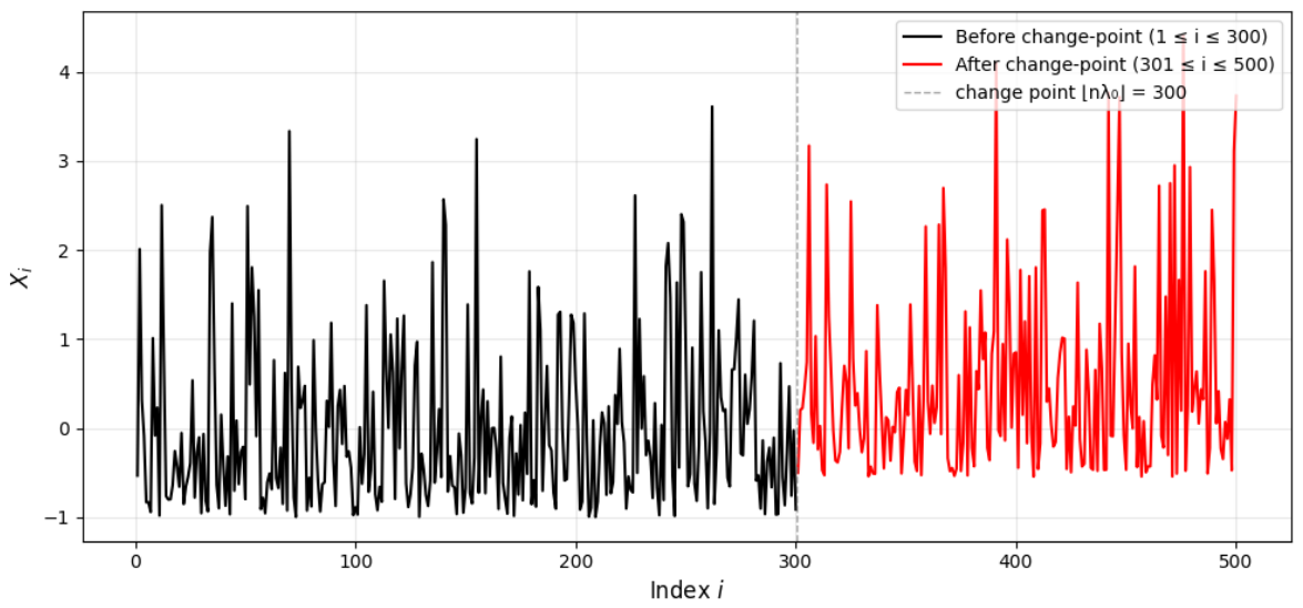
X i = ε i − 1 if 1 ≤ i ≤ 300 ε i − 1 + γ . n − 1 / 2 if 301 ≤ i ≤ 500
with γ · n − 1 / 2 = 10 / 500 ≈ 0.4472 .
We thus have the theoretical moments:
  • Before change: E [ X i ] = 1 − 1 = 0 , Var ( X i ) = 1 ;
  • After change: E [ X i ] = 0.4472 , Var ( X i ) = 1 .
The trajectories of the considered random variables are described in this Figure 1.
Figure 1. Shows the simulation of the trajectories of X i before the change point (in black) and after the change point (in red).
We use the Gaussian kernel for l = 3 defined by
ϕ ( x 1 , x 2 , x 3 ) = exp − x 1 2 + x 2 2 + x 3 2 2
This kernel is bounded: 0 < ϕ ≤ 1 , symmetric by permutation and differentiable.
Then we have
Θ ϕ ( 3 ) ( F , F ) = ∫ − 1 + ∞ e − x 2 / 2 · e − ( x + 1 ) d x 3 ≈ ( 0.760 ) 3 ≈ 0.439 ,
and
σ 2 = E [ ϕ 1 ( X 1 ) 2 ]
where ϕ 1 is the Hoeffding projection of order 1:
ϕ 1 ( x ) = E [ ϕ ( x , X 2 , X 3 ) ] − Θ ϕ ( 3 ) ( F , F )
Numerical estimation: σ 2 ≈ 0.045 .
We now show the simulations results of Theorems 1 and 2:

4.1. Theorem 1 (A0: No Change)

n 1 / 2 − l U [ n λ ] ( l ) converges in distribution to
U λ = 1 2 ( 1 − 2 λ ) W ( λ ) + ( 2 λ − λ 2 ) W ( 1 )
  • Mean: 0 for any λ ∈ [ 0 , 1 ] ;
  • Covariance: Cov ( W ( λ 1 ) , W ( λ 2 ) ) = min ( λ 1 , λ 2 ) · σ 2 .
Theoretical variance at λ :
Var ( U λ ) = σ 2 4 ( 1 − 2 λ ) 2 λ + ( 2 λ − λ 2 ) 2 + 2 ( 1 − 2 λ ) ( 2 λ − λ 2 ) λ

4.2. Theorem 2 (A1,n: Weak Change)

n 1 / 2 − l U [ n λ ] ( l ) converges in distribution to
U ˜ λ = λ 2 ( 1 − λ ) 2 · C ︸ Mean + ( 1 − λ ) 2 2 W 1 ( λ ) + λ 2 2 [ W 2 ( 1 ) − W 2 ( λ ) ] ︸ Fluctuations
Theoretical mean function:
μ ( λ ) = λ 2 ( 1 − λ ) 2 · C ≈ − 0.095 · λ 2 ( 1 − λ )
Theoretical variance function:
Var ( U ˜ λ ) = σ 2 4 λ ( 1 − λ ) 4 + ( 1 − λ ) λ 4 = σ 2 λ ( 1 − λ ) 4 ( 1 − λ ) 3 + λ 3 , 0 ≤ λ ≤ 1 .
The constant C is
C = 1 2 ∑ j = 1 2 ∑ i = j + 1 3 ( − γ ) ∫ … ∫ ∂ ϕ ∂ u i ∏ f ( x ) d x ≈ 2 2 × 3 × ( − 0.15 ) × ( 0.655 ) 2 ≈ − 0.19 ,
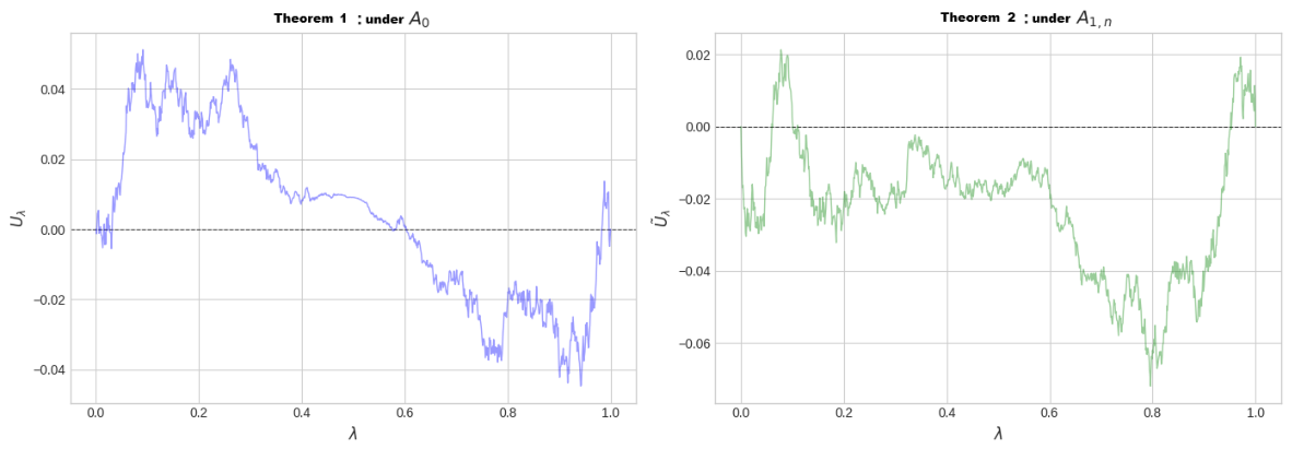
The results are illustrated in this Figure 2.
Figure 2. First row: no change-point and mean μ = 0 , and second row: change-point at n = 300 and mean μ ( λ ) = − 0.095 λ 2 ( 1 − λ ) .
The figure shows the limit Brownian bridges of each theorem. It clearly shows that under the hypothesis A 0 , the empirical mean is almost zero. We have almost a balance of values according to the value of λ . This validates our condition and the result of Theorem 1.
Under the hypothesis A 1 , n , with the choice of positive γ , the value of C is negative. This choice affects the values of our estimator and leads to negative values of the limit process. The expression of the mean μ ( λ ) guarantees this statement. As C is negative, for all λ ∈ [ 0 , 1 ] , μ ( λ ) has almost negative values. Therefore, if we calculate the empirical mean, we will obtain a negative value. This figure clearly shows this value.
In these simulations, we considered random variables whose mean changes at [ n λ 0 ] .

5. Conclusions

Considering a sequence of absolutely continuous i.i.d random variables X 1 , … , X n , we study the asymptotic properties, in the case of the existence or not of a change point, of the estimators Z n , [ n λ ] ( l ) and the sequence of processes U [ n λ ] ( l ) based on U-statistics with a kernel of degree more than two. The asymptotic normality of U [ n λ ] ( l ) , with the same convergence speed n − 1 / 2 , is established under A 0 and A 1 , n (with weak changes). The almost sure convergence of Z n , [ n λ ] ( l ) , with the same convergence speed n − l , is also obtained under A 0 and A 1 . The generalization of our results in the case of multi-change points and the consideration of mixing random variables are interesting prospects for future research.

Author Contributions

Conceptualization, J.R., V.H. and M.H.; methodology, J.R., V.H. and M.H.; software, J.R., V.H. and M.H.; writing—original draft preparation, J.R., V.H. and M.H.; writing—review and editing, J.R., V.H. and M.H.; supervision, V.H. and M.H.; validation, V.H. and M.H. All authors have read and agreed to the published version of the manuscript.

Funding

This research received no external funding.

Data Availability Statement

No new data were created or analyzed in this study.

Acknowledgments

The authors would like to thank the Editor and the Reviewers for their comments which allow them to improve the manuscript.

Conflicts of Interest

The authors declare no conflicts of interest.

Appendix A. Proofs of Results

To simplify the notations, denote:
∑ ( n , j , λ ) the   summation   over   the   set ( i 1 , … , i j ) / 1 ⩽ i 1 < … < i j ⩽ [ n λ ] , 0 ⩽ λ ⩽ 1 ,
∑ ( n , j , λ * ) the   summation   over   the   set ( i j + 1 , … , i d ) / [ n λ ] + 1 ⩽ i j + 1 < … < i d ⩽ n , j < d ⩽ l ,
∑ ( n , j , λ 1 , λ 2 ) the   summation   over   the   set ( i 1 , … , i j ) / [ n λ 1 ] + 1 ⩽ i 1 < … < i j ⩽ [ n λ 2 ] , λ 1 ⩽ λ 2 ,
∑ ( n , j , λ 1 * , λ 2 ) the   summation   over   the   set ( i j + 1 , … , i d ) / [ n λ 1 ] + 1 ⩽ i j + 1 < … < i d ⩽ [ n λ 2 ] ,
and ∑ ( n , 0 , λ 1 * , λ 2 ) the   summation   over   the   set ( i 1 , … , i d ) / [ n λ 1 ] + 1 ⩽ i 1 < … < i d ⩽ [ n λ 2 ] .
By convention, ∑ ( n , 0 , λ ) = ⌀ , ∑ ( n , 0 , λ * ) is the summation over the set
( i 1 , … , i d ) / [ n λ ] + 1 ⩽ i 1 < … < i d ⩽ n ; ∑ ( n , d , λ ) is the summation over the set
( i 1 , … , i d ) / 1 ⩽ i 1 < … < i d ⩽ [ n λ ] and ∑ ( n , d , λ * ) = ⌀ .

Appendix A.1. Proof of Theorem 1

Taking k = [ n λ ] in the relations (2) and (4), under A 0 , we have:
n 1 2 − l U [ n λ ] ( l ) = n 1 2 − l ∑ j = 1 l − 1 ∑ ( n , j , λ ) ∑ ( n , j , λ * ) ϕ X i 1 , … , X i j , X i j + 1 , … , X i l − Θ ϕ ( l ) ( F , F ) = n 1 2 − l ∑ ( n , l , 1 ) ϕ ( X i 1 , … , X i l ) − Θ ϕ ( l ) ( F , F ) − n 1 2 − l ∑ ( n , l , λ ) ϕ ( X i 1 , … , X i l ) − Θ ϕ ( l ) ( F , F ) + ∑ ( n , 0 , λ * ) ϕ ( X i 1 , … , X i l ) − Θ ϕ ( l ) ( F , F )
From the Hoeffding decomposition, we have
n l − 1 ∑ ( n , l , 1 ) ( ϕ ( X i 1 , … , X i l ) − Θ ϕ ( l ) ( F , F ) ) = ∑ c = 0 l l c n c − 1 ∑ ( n , c , 1 ) ϕ c ( X i 1 , … , X i c ) .
[ n λ ] l − 1 ∑ ( n , l , λ ) ( ϕ ( X i 1 , … , X i l ) − Θ ϕ ( l ) ( F , F ) ) = ∑ c = 0 l l c [ n λ ] c − 1 ∑ ( n , c , λ ) ϕ c ( X i 1 , … , X i c ) .
n − [ n λ ] l − 1 ∑ ( n , 0 , λ * ) ( ϕ ( X i 1 , … , X i l ) − Θ ϕ ( l ) ( F , F ) ) = ∑ c = 0 l l c n − [ n λ ] c − 1 ∑ ( n , 0 , λ * ) ϕ c ( X i 1 , … , X i c ) .
Consequently, for c = 0 , the function ϕ 0 is identically equal to zero; then, we have
n 1 2 − l U [ n λ ] ( l ) = n 1 2 − l n l l 1 n 1 − 1 ∑ ( n , 1 , 1 ) ϕ 1 ( X i 1 ) − n 1 2 − l [ n λ ] l l 1 [ n λ ] 1 − 1 ∑ ( n , 1 , λ ) ϕ 1 ( X i 1 ) − n 1 2 − l n − [ n λ ] l l 1 n − [ n λ ] 1 − 1 ∑ ( n , 0 , λ * ) ϕ 1 ( X i 1 ) + n 1 2 − l n l ∑ c = 2 l l c n c − 1 ∑ ( n , c , 1 ) ϕ c ( X i 1 , … , X i c ) − n 1 2 − l [ n λ ] l ∑ c = 2 l l c [ n λ ] c − 1 ∑ ( n , c , λ ) ϕ c ( X i 1 , … , X i c ) − n 1 2 − l n − [ n λ ] l ∑ c = 2 l l c n − [ n λ ] c − 1 ∑ ( n , 0 , λ * ) ϕ c ( X i 1 , … , X i c )
After some calculations, we obtain
n 1 2 − l U [ n λ ] ( l ) = A n , λ ( l ) + B n , λ ( l ) ,
where
A n , λ ( l ) = n 1 2 − l . ( n − 1 ) … ( n − l + 1 ) ( l − 1 ) ! − n 1 2 − l . ( [ n λ ] − 1 ) … ( [ n λ ] − l + 1 ) ( l − 1 ) ! ∑ ( n , 1 , λ ) ϕ 1 ( X i 1 ) + n 1 2 − l . ( n − 1 ) … ( n − l + 1 ) ( l − 1 ) ! − n 1 2 − l . ( n − [ n λ ] − 1 ) … ( n − [ n λ ] − l + 1 ) ( l − 1 ) ! ∑ ( n , 1 , λ * ) ϕ 1 ( X i 1 )
and
B n , λ ( l ) = n 1 2 − l n l ∑ c = 2 l l c n c − 1 ∑ ( n , c , 1 ) ϕ c ( X i 1 , … , X i c ) − n 1 2 − l [ n λ ] l ∑ c = 2 l l c [ n λ ] c − 1 ∑ ( n , c , λ ) ϕ c ( X i 1 , … , X i c ) − n 1 2 − l n − [ n λ ] l ∑ c = 2 l l c n − [ n λ ] c − 1 ∑ ( n , 0 , λ * ) ϕ c ( X i 1 , … , X i c )
We then show that B n , λ ( l ) converges in probability to zero and A n , λ ( l ) converges in distribution towards a Gaussian process as n tends to infinity.
Proposition A1. 
Assuming that the conditions of Theorem 1 hold, we have, in probability
sup 0 ⩽ λ ⩽ 1 | B n , λ ( l ) | ⟶ n → ∞ 0 .
Proof. 
We need the following lemmas.
Lemma A1. 
Assuming that the conditions of Theorem 1 hold, we have
E | n l − 1 / 2 B n , λ ( l ) | 2 ⩽ C s t . [ n λ ] l − 1 ( n − [ n λ ] ) l − 1 .
Proof. 
We have
E ( n l − 1 / 2 B n , λ ( l ) ) 2 = E ∑ c = 2 l l c n l n c − 1 ∑ ( n , c , 1 ) ϕ c ( X i 1 , … , X i c ) − [ n λ ] l [ n λ ] c − 1 ∑ ( n , c , λ ) ϕ c ( X i 1 , … , X i c ) − n − [ n λ ] l n − [ n λ ] c − 1 ∑ ( n , 0 , λ * ) ϕ c ( X i 1 , … , X i c ) 2 = E l 2 n l n 2 − 1 ∑ ( n , 2 , 1 ) ϕ 2 ( X i 1 , X i 2 ) − [ n λ ] l [ n λ ] 2 − 1 ∑ ( n , 2 , λ ) ϕ 2 ( X i 1 , X i 2 ) − n − [ n λ ] l n − [ n λ ] 2 − 1 ∑ ( n , 0 , λ * ) ϕ 2 ( X i 1 , X i 2 ) + l 3 n l n 3 − 1 ∑ ( n , 3 , 1 ) ϕ 3 ( X i 1 , X i 2 , X i 3 ) − [ n λ ] l [ n λ ] 3 − 1 ∑ ( n , 3 , λ ) ϕ 3 ( X i 1 , X i 2 , X i 3 ) − n − [ n λ ] l n − [ n λ ] 3 − 1 ∑ ( n , 0 , λ * ) ϕ 3 ( X i 1 , X i 2 , X i 3 ) + … + l l − 1 n l n l − 1 − 1 ∑ ( n , l − 1 , 1 ) ϕ l − 1 ( X i 1 , … , X i l − 1 ) − [ n λ ] l [ n λ ] l − 1 − 1 ∑ ( n , l − 1 , λ ) ϕ l − 1 ( X i 1 , … , X i l − 1 ) − n − [ n λ ] l n − [ n λ ] l − 1 − 1 ∑ ( n , 0 , λ * ) ϕ l − 1 ( X i 1 , … , X i l − 1 ) + ∑ ( n , l , 1 ) ϕ l ( X i 1 , … , X i l ) − ∑ ( n , l , λ ) ϕ l ( X i 1 , … , X i l ) − ∑ ( n , 0 , λ * ) ϕ l ( X i 1 , … , X i l ) 2 ,
This expression is valid for any l > 2 . As l is finite and condition (9) is satisfied, to simplify the calculations and without loss of generality, we prove it for l = 3 ,
E ( n 5 / 2 B n , λ ( 3 ) ) 2 = E ∑ c = 2 3 3 c n 3 n c − 1 ∑ ( n , c , 1 ) ϕ c ( X i 1 , … , X i c ) − [ n λ ] 3 [ n λ ] c − 1 ∑ ( n , c , λ ) ϕ c ( X i 1 , … , X i c ) − n − [ n λ ] 3 n − [ n λ ] c − 1 ∑ ( n , 0 , λ * ) ϕ c ( X i 1 , … , X i c ) 2
= E 3 2 n 3 n 2 − 1 ∑ ( n , 2 , 1 ) ϕ 2 ( X i 1 , X i 2 ) − [ n λ ] 3 [ n λ ] 2 − 1 ∑ ( n , 2 , λ ) ϕ 2 ( X i 1 , X i 2 ) − n − [ n λ ] 3 n − [ n λ ] 2 − 1 ∑ ( n , 0 , λ * ) ϕ 2 ( X i 1 , X i 2 ) + ∑ ( n , 3 , 1 ) ϕ 3 ( X i 1 , X i 2 , X i 3 ) − ∑ ( n , 3 , λ ) ϕ 3 ( X i 1 , X i 2 , X i 3 ) − ∑ ( n , 0 , λ * ) ϕ 3 ( X i 1 , X i 2 , X i 3 ) 2 ,
According to relation (4) and using the well-known inequality
( a + b + c + d + e ) 2 ⩽ 5 ( a 2 + b 2 + c 2 + d 2 + e 2 ) ,
we have
E ( n 5 / 2 B n , λ ( 3 ) ) 2 = E 3 2 n 3 n 2 − 1 ∑ ( n , 2 , 1 ) ϕ 2 ( X i 1 , X i 2 ) − [ n λ ] 3 [ n λ ] 2 − 1 ∑ ( n , 2 , λ ) ϕ 2 ( X i 1 , X i 2 ) − n − [ n λ ] 3 n − [ n λ ] 2 − 1 ∑ ( n , 0 , λ * ) ϕ 2 ( X i 1 , X i 2 ) + ∑ j = 1 2 ∑ ( n , j , λ ) ∑ ( n , 0 , λ * ) ϕ 3 ( X i 1 , … , X i j , X i j + 1 , … , X i 3 ) 2 = E ( n − 2 ) ∑ ( n , 2 , 1 ) ϕ 2 ( X i 1 , X i 2 ) − ∑ ( n , 2 , λ ) ϕ 2 ( X i 1 , X i 2 ) − ∑ ( n , 0 , λ * ) ϕ 2 ( X i 1 , X i 2 ) + ( n − [ n λ ] ) ∑ ( n , 2 , λ ) ϕ 2 ( X i 1 , X i 2 ) + [ n λ ] ∑ ( n , 0 , λ * ) ϕ 2 ( X i 1 , X i 2 ) + ∑ ( n , 1 , λ ) ∑ ( n , 1 , λ * ) ϕ 3 ( X i 1 , X i 2 , X i 3 ) + ∑ ( n , 2 , λ ) ∑ ( n , 2 , λ * ) ϕ 3 ( X i 1 , X i 2 , X i 3 ) 2 ⩽ 5 . ( n − 2 ) 2 E ∑ ( n , 1 , λ ) ∑ ( n , 1 , λ * ) ϕ 2 ( X i 1 , X i 2 ) 2 + 5 . ( n − [ n λ ] ) 2 E ∑ ( n , 2 , λ ) ϕ 2 ( X i 1 , X i 2 ) 2 + 5 . [ n λ ] 2 E ∑ ( n , 0 , λ * ) ϕ 2 ( X i 1 , X i 2 ) 2 + 5 . E ∑ ( n , 1 , λ ) ∑ ( n , 1 , λ * ) ϕ 3 ( X i 1 , X i 2 , X i 3 ) 2 + 5 . E ∑ ( n , 2 , λ ) ∑ ( n , 2 , λ * ) ϕ 3 ( X i 1 , X i 2 , X i 3 ) 2 .
From the Cauchy–Schwartz inequality and condition (9), we obtain
E ( n 5 / 2 B n , λ ( 3 ) ) 2 ⩽ C s t . ( n − 2 ) 2 . [ n λ ] ( n − [ n λ ] ) + ( n − [ n λ ] ) 2 . [ n λ ] ( [ n λ ] − 1 ) 2 + [ n λ ] 2 . ( n − [ n λ ] ) ( n − [ n λ ] − 1 ) 2 + [ n λ ] ( n − [ n λ ] ) ( n − [ n λ ] − 1 ) 2 + [ n λ ] ( [ n λ ] − 1 ) ( n − [ n λ ] ) 2
⩽ C s t . [ n λ ] ( n − [ n λ ] ) ( n − 2 ) 2 + [ n λ ] ( n − [ n λ ] ) − 1 ⩽ C s t . [ n λ ] 2 ( n − [ n λ ] ) 2 .
Hence Lemma A1 is proved. □
Lemma A2.  
Assuming that the conditions of Theorem 1 hold, we have, for 0 ⩽ λ 1 ⩽ λ 2 ⩽ 1 ,
E | B n , λ 2 ( l ) − B n , λ 1 ( l ) | 2 ⩽ C s t . ( λ 2 − λ 1 ) n .
Proof. 
Since l is finite and the condition (9) is satisfied, as the proof of Lemma A1, we prove it for l = 3 ,
E | B n , λ 2 ( 3 ) − B n , λ 1 ( 3 ) | 2 = 1 n 5 E ∑ c = 2 3 3 c n 3 n c − 1 ∑ ( n , c , 1 ) ϕ c ( X i 1 , … , X i c ) − [ n λ 2 ] 3 [ n λ 2 ] c − 1 ∑ ( n , c , λ 2 ) ϕ c ( X i 1 , … , X i c ) − n − [ n λ 2 ] 3 n − [ n λ 2 ] c − 1 ∑ ( n , 0 , λ 2 * ) ϕ c ( X i 1 , … , X i c ) − ∑ c = 2 3 3 c n 3 n c − 1 ∑ ( n , c , 1 ) ϕ c ( X i 1 , … , X i c ) − [ n λ 1 ] 3 [ n λ 1 ] c − 1 ∑ ( n , c , λ 1 ) ϕ c ( X i 1 , … , X i c ) − n − [ n λ 1 ] 3 n − [ n λ 1 ] c − 1 ∑ ( n , 0 , λ 1 * ) ϕ c ( X i 1 , … , X i c ) 2 = 1 n 5 E ( n − 2 ) ∑ ( n , 2 , 1 ) ϕ 2 ( X i 1 , X i 2 ) − ( [ n λ 2 ] − 2 ) ∑ ( n , 2 , λ 2 ) ϕ 2 ( X i 1 , X i 2 ) − ( n − [ n λ 2 ] − 2 ) ∑ ( n , 0 , λ 2 * ) ϕ 2 ( X i 1 , X i 2 ) + ∑ j = 1 2 ∑ ( n , j , λ 2 ) ∑ ( n , 0 , λ 2 * ) ϕ 3 ( X i 1 , … , X i j , … , X i 3 ) − ( n − 2 ) ∑ ( n , 2 , 1 ) ϕ 2 ( X i 1 , X i 2 ) − ( [ n λ 1 ] − 2 ) ∑ ( n , 2 , λ 1 ) ϕ 2 ( X i 1 , X i 2 ) − ( n − [ n λ 1 ] − 2 ) ∑ ( n , 0 , λ 1 * ) ϕ 2 ( X i 1 , X i 2 ) − ∑ j = 1 2 ∑ ( n , j , λ 1 ) ∑ ( n , 0 , λ 1 * ) ϕ 3 ( X i 1 , … , X i j , … , X i 3 ) 2
⩽ 1 n 5 E ( n − 2 ) ∑ ( n , 1 , λ 2 ) ∑ ( n , 1 , λ 2 * ) ϕ 2 ( X i 1 , X i 2 ) − ∑ ( n , 1 , λ 1 ) ∑ ( n , 1 , λ 1 * ) ϕ 2 ( X i 1 , X i 2 ) + [ n λ 2 ] ∑ ( n , 0 , λ 2 * ) ϕ 2 ( X i 1 , X i 2 ) − [ n λ 1 ] ∑ ( n , 0 , λ 1 * ) ϕ 2 ( X i 1 , X i 2 ) − ( n − [ n λ 2 ] ) ∑ ( n , 2 , λ 2 ) ϕ 2 ( X i 1 , X i 2 ) − ( n − [ n λ 1 ] ) ∑ ( n , 2 , λ 1 ) ϕ 2 ( X i 1 , X i 2 ) + ∑ j = 1 2 ∑ ( n , j , λ 2 ) ∑ ( n , 0 , λ 2 * ) ϕ 3 ( X i 1 , … , X i j , … , X i 3 ) − ∑ j = 1 2 ∑ ( n , j , λ 1 ) ∑ ( n , 0 , λ 1 * ) ϕ 3 ( X i 1 , … , X i j , … , X i 3 ) 2 ⩽ 10 n 5 ( n − 2 ) 2 E ∑ ( n , 1 , λ 2 ) ∑ ( n , 1 , λ 2 * ) ϕ 2 ( X i 1 , X i 2 ) − ∑ ( n , 1 , λ 1 ) ∑ ( n , 1 , λ 1 * ) ϕ 2 ( X i 1 , X i 2 ) 2 + [ n λ 2 ] − [ n λ 1 ] 2 E ∑ ( n , 0 , λ 2 * ) ϕ 2 ( X i 1 , X i 2 ) 2 + [ n λ 1 ] 2 E ∑ ( n , 1 , λ 1 , λ 2 ) ∑ ( n , 1 , λ 2 * ) ϕ 2 ( X i 1 , X i 2 ) 2 + [ n λ 2 ] ) − [ n λ 1 ] 2 E ∑ ( n , 2 , λ 1 ) ϕ 2 ( X i 1 , X i 2 ) 2 + ( n − [ n λ 2 ] ) 2 E ∑ ( n , 2 , λ 1 * , λ 2 ) ϕ 2 ( X i 1 , X i 2 ) 2 + ( n − [ n λ 2 ] − [ n λ 1 ] ) 2 E ∑ ( n , 1 , λ 1 ) ∑ ( n , 1 , λ 1 * , λ 2 ) ϕ 2 ( X i 1 , X i 2 ) 2 + E ∑ ( n , 1 , λ 1 ) ∑ ( n , 1 , λ 1 * , λ 2 ) ϕ 3 ( X i 1 , X i 2 , X i 3 ) 2 + E ∑ ( n , 1 , λ 1 , λ 2 ) ∑ ( n , 1 , λ 2 * ) ϕ 3 ( X i 1 , X i 2 , X i 3 ) 2 + E ∑ ( n , 2 , λ 1 ) ∑ ( n , 2 , λ 1 * , λ 2 ) ϕ 3 ( X i 1 , X i 2 , X i 3 ) 2 + E ∑ ( n , 2 , λ 1 , λ 2 ) ∑ ( n , 2 , λ 2 * ) ϕ 3 ( X i 1 , X i 2 , X i 3 ) 2 .
From the Cauchy–Schwartz inequality and condition (9), we have
E | B n , λ 2 ( 3 ) − B n , λ 1 ( 3 ) | 2 ⩽ 10 n 5 C s t ( n − 2 ) 2 [ n λ 1 ] ( [ n λ 2 ] − [ n λ 1 ] ) + ( [ n λ 2 ] − [ n λ 1 ] ) ( n − [ n λ 1 ] ) + ( [ n λ 2 ] − [ n λ 1 ] ) 2 ( n − [ n λ 2 ] ) ( n − [ n λ 2 ] − 1 ) 2 + [ n λ 1 ] 2 ( [ n λ 2 ] − [ n λ 1 ] ) ( n − [ n λ 1 ] ) 2 + ( [ n λ 2 ] − [ n λ 1 ] ) 2 [ n λ 1 ] ( [ n λ 1 ] − 1 ) 2 + ( n − [ n λ 2 ] − [ n λ 1 ] ) 2 ( [ n λ 2 ] − [ n λ 1 ] ) ( [ n λ 2 ] − [ n λ 1 ] − 1 ) 2 + ( n − [ n λ 2 ] ) 2 [ n λ 1 ] ( [ n λ 2 ] − [ n λ 1 ] ) + [ n λ 1 ] ( [ n λ 2 ] − [ n λ 1 ] ) ( [ n λ 2 ] − [ n λ 1 ] − 1 ) 2
+ ( [ n λ 2 ] − [ n λ 1 ] ) ( n − [ n λ 2 ] ) ( n − [ n λ 2 ] − 1 ) 2 + ( [ n λ 2 ] − [ n λ 1 ] ) [ n λ 1 ] ( [ n λ 1 ] − 1 ) 2 + ( [ n λ 2 ] − [ n λ 1 ] ) ( [ n λ 2 ] − [ n λ 1 ] − 1 ) 2 ( n − [ n λ 2 ] ) ⩽ C s t . ( λ 2 − λ 1 ) n .
Hence Lemma A2 is proved. □
Let us return to the proof of the Proposition A1. By Chebychev’s inequality and Lemma A2, we have
P B n , λ 2 ( l ) − B n , λ 1 ( l ) ⩾ ϵ ⩽ 1 ϵ 2 E B n , λ 2 ( l ) − B n , λ 1 ( l ) 2 ⩽ C s t . ( λ 2 − λ 1 ) ϵ 2 n ,
for all ϵ > 0 .
We deduce for 0 ⩽ n 1 ⩽ n 2 ⩽ n with n 1 , n 2 , n ∈ N ,
P B n , n 2 n ( l ) − B n , n 1 n ( l ) ⩾ ϵ ⩽ C s t . ( n 2 − n 1 ) ϵ 2 n 2 ⩽ C s t . ( n 2 − n 1 ) 4 / 3 ϵ 2 n 5 / 3 .
Now, consider the partial sum process τ i = B n , i n ( l ) − B n , i − 1 n ( l ) if i = 1 , … , n − 1 , and τ 0 = 0 . Denote S i = τ 1 + τ 2 + … + τ i with S 0 = 0 . Then S i = B n , i n ( l ) .
The inequalities (A1) are equivalent to
P S n 2 − S n 1 ⩾ ϵ ⩽ C s t ϵ 2 n 2 − n 1 n 5 / 4 4 / 3 .
From Theorem 10.2 of Billingsley [17], we deduce
P max 1 ⩽ i ⩽ n − 1 | S i | ⩾ ϵ ⩽ C s t ϵ 2 n 2 − n 1 n 5 / 4 4 / 3 ⩽ C s t ϵ 2 n 1 / 3 .
Finally, we have, in probability,
sup 0 ⩽ λ ⩽ 1 | B n , λ ( l ) | ⟶ n → ∞ 0 .
□
Now, we show that A n , λ ( l ) converges in distribution towards a Gaussian process as n tends to infinity. A n , λ ( l ) can be written
A n , λ ( l ) = n 1 2 − l ∏ a = 1 l − 1 ( n − a ) ( l − 1 ) ! − ∏ a = 1 l − 1 ( [ n λ ] − a ) ( l − 1 ) ! ∑ ( n , 1 , λ ) ϕ 1 ( X i 1 ) + n 1 2 − l ∏ a = 1 l − 1 ( n − a ) ( l − 1 ) ! − ∏ a = 1 l − 1 ( n − [ n λ ] − a ) ( l − 1 ) ! ∑ ( n , 1 , 1 ) ϕ 1 ( X i 1 ) − ∑ ( n , 1 , λ ) ϕ 1 ( X i 1 )
= n 1 2 − l ∏ a = 1 l − 1 ( n − [ n λ ] − a ) ( l − 1 ) ! − ∏ a = 1 l − 1 ( [ n λ ] − a ) ( l − 1 ) ! ∑ ( n , 1 , λ ) ϕ 1 ( X i 1 ) + n 1 2 − l ∏ a = 1 l − 1 ( n − a ) ( l − 1 ) ! − ∏ a = 1 l − 1 ( n − [ n λ ] − a ) ( l − 1 ) ! ∑ ( n , 1 , 1 ) ϕ 1 ( X i 1 ) .
From Theorem 8.2 of Billingsley [17], we have
1 n 1 / 2 ∑ ( n , 1 , λ ) ϕ 1 ( X i 1 ) ⟶ D n → ∞ W ( λ ) ,
1 n 1 / 2 ∑ ( n , 1 , 1 ) ϕ 1 ( X i l ) ⟶ D n → ∞ W ( 1 ) .
We also have, for 1 ⩽ a ⩽ l − 1 ,
∏ a = 1 l − 1 ( n − [ n λ ] − a ) n l − 1 − ∏ a = 1 l − 1 ( [ n λ ] − a ) n l − 1 ⟶ n → ∞ ( 1 − λ ) l − 1 − λ l − 1 ,
∏ a = 1 l − 1 ( n − a ) n l − 1 − ∏ a = 1 l − 1 ( n − [ n λ ] − a ) n l − 1 ⟶ n → ∞ 1 − ( 1 − λ ) l − 1 .
So by Slutsky’s lemma, we have:
A n , λ ( l ) ⟶ D n → ∞ U λ ( l ) ,
with
U λ ( l ) = 1 ( l − 1 ) ! ( 1 − λ ) l − 1 − λ l − 1 W ( λ ) + ( 1 − ( 1 − λ ) l − 1 ) W ( 1 ) , 0 ⩽ λ ⩽ 1 .
This completes the proof of Theorem 1.

Appendix A.2. Proof of Theorem 2

From A 1 , n and ( C 3 ) , we have
n 1 2 − l U [ n λ ] ( l ) = n 1 2 − l Z n , [ n λ ] ( l ) − n 1 2 − l ∑ j = 1 l − 1 [ n λ ] j n − [ n λ ] l − j Θ ϕ ( l ) ( F , F ) = n 1 2 − l ∑ j = 1 l − 1 ∑ ( n , j , λ ) ∑ ( n , j , λ * ) ϕ ( X i 1 , … , X i j , Y n i j + 1 , … , Y n i l ) − n 1 2 − l ∑ j = 1 l − 1 [ n λ ] j n − [ n λ ] l − j Θ ϕ ( l ) ( F , F )
and
∑ ( n , j , λ ) ∑ ( n , j , λ * ) ϕ ( X i 1 , … , X i j , Y n i j + 1 , … , Y n i l ) = [ n λ ] j n − [ n λ ] l − j [ n λ ] j − 1 n − [ n λ ] l − j − 1 × ∑ ( n , j , λ ) ∑ ( n , j , λ * ) ϕ ( X i 1 , … , X i j , Y n i j + 1 , … , Y n i l ) .
Denote
D n , j = [ n λ ] j − 1 n − [ n λ ] l − j − 1 ∑ ( n , j , λ ) ∑ ( n , j , λ * ) ϕ ( X i 1 , … , X i j , Y n i j + 1 , … , Y n i l ) .
From the proof of Theorem 2.2 of Sen [18], we have
D n , j = Θ ϕ ( l ) ( F , G ( n ) ) + D 1 , n , j + D 2 , n , j + D 3 , n , j
where
D 1 , n , j = [ n λ ] j − 1 ∑ ( n , j , λ ) ϕ j , 0 ( X i 1 , … , X i j ) ,
D 2 , n , j = n − [ n λ ] l − j − 1 ∑ ( n , j , λ * ) ϕ 0 , ( l − j ) ( Y n i j + 1 , … , Y n i l ) ,
D 3 , n , j = ∑ d 1 = 1 j ∑ d 2 = 1 l − j j d 1 l − j d 2 ∑ c 1 = 1 d 1 ∑ c 2 = 1 d 2 ( − 1 ) c 1 + c 2 d 1 c 1 d 2 c 2 [ n λ ] c 1 − 1 n − [ n λ ] c 2 − 1 × ∑ ( n ) * ϕ c 1 , c 2 ( X i 1 , … , X i c 1 , Y n i j + 1 , … , Y n i j + c 2 ) ,
with ϕ j , 0 , ϕ 0 , l − j and ϕ c 1 , c 2 defined in (6)–(8) respectively, and ∑ ( n ) * is the summation over the set
( i 1 , … , i c 1 , i j + 1 , … , i j + c 2 ) / 1 ⩽ i 1 < … < i c 1 ⩽ [ n λ ] , [ n λ ] + 1 ⩽ i j + 1 < … < i c 2 ⩽ n .
Now, we have
n 1 2 − l U [ n λ ] ( l ) = n 1 2 − l ∑ j = 1 l − 1 [ n λ ] j n − [ n λ ] l − j D n , j − n 1 2 − l ∑ j = 1 l − 1 [ n λ ] j n − [ n λ ] l − j Θ ϕ ( l ) ( F , F ) = n 1 2 − l ∑ j = 1 l − 1 [ n λ ] j n − [ n λ ] l − j { Θ ϕ ( l ) ( F , G ( n ) ) + D 1 , n , j + D 2 , n , j + D 3 , n , j } − n 1 2 − l ∑ j = 1 l − 1 [ n λ ] j n − [ n λ ] l − j Θ ϕ ( l ) ( F , F ) = M n + N n
where
M n = n 1 2 − l ∑ j = 1 l − 1 [ n λ ] j n − [ n λ ] l − j { Θ ϕ ( l ) ( F , G ( n ) ) − Θ ϕ ( l ) ( F , F ) } + n 1 2 − l [ n λ ] 1 n − [ n λ ] l − 1 D 1 , n , 1 + n 1 2 − l [ n λ ] l − 1 n − [ n λ ] 1 D 2 , n , l − 1 ,
N n = n 1 2 − l ∑ j = 2 l − 1 [ n λ ] j n − [ n λ ] l − j D 1 , n , j + n 1 2 − l ∑ j = 1 l − 2 [ n λ ] j n − [ n λ ] l − j D 2 , n , j + n 1 2 − l ∑ j = 1 l − 1 [ n λ ] j n − [ n λ ] l − j D 3 , n , j .
By applying Chebychev inequality to N n , we have, for all ϵ > 0 ,
P ( N n > ϵ ) ⩽ 1 ϵ 2 E ( N n 2 ) .
From condition (10) and Theorem 2.2 of Sen [18], we deduce
E ( N n 2 ) = n 1 − 2 l ∑ j = 2 l − 1 [ n λ ] j 2 n − [ n λ ] l − j 2 O ( n − 2 ) + n 1 − 2 l ∑ j = 1 l − 2 [ n λ ] j 2 n − [ n λ ] l − j 2 O ( n − 2 ) + n 1 − 2 l ∑ j = 1 l − 1 [ n λ ] j 2 n − [ n λ ] l − j 2 ∑ d 1 = 1 j ∑ d 2 = 1 l − j j d 1 2 l − j d 2 2 × ∑ c 1 = 1 d 1 ∑ c 2 = 1 d 2 ( − 1 ) 2 ( c 1 + c 2 ) d 1 c 1 2 d 2 c 2 2 O ( n − 2 ) .
As
[ n λ ] j 2 n − [ n λ ] l − j 2 = O ( n 2 l ) ,
the term
n − 2 l ∑ j = 2 l − 1 [ n λ ] j 2 n − [ n λ ] l − j 2 + n − 2 l ∑ j = 1 l − 2 [ n λ ] j 2 n − [ n λ ] l − j 2 + n − 2 l ∑ j = 1 l − 1 [ n λ ] j 2 n − [ n λ ] l − j 2 ∑ d 1 = 1 j ∑ d 2 = 1 l − j j d 1 2 l − j d 2 2 × ∑ c 1 = 1 d 1 ∑ c 2 = 1 d 2 ( − 1 ) 2 ( c 1 + c 2 ) d 1 c 1 2 d 2 c 2 2
converges to a constant as n tends to infinity. Then E ( N n 2 ) tends to zero as n tends to infinity.
Hence N n converges in probability to zero as n tends to infinity.
Now, we show the convergence in distribution of M n .
M n = n 1 2 − l ∑ j = 1 l − 1 [ n λ ] j n − [ n λ ] l − j { Θ ϕ ( l ) ( F , G ( n ) ) − Θ ϕ ( l ) ( F , F ) } + n 1 2 − l [ n λ ] 1 n − [ n λ ] l − 1 [ n λ ] 1 − 1 ∑ i 1 = 1 [ n λ ] ϕ 1 , 0 ( X i 1 ) + n 1 2 − l [ n λ ] l − 1 n − [ n λ ] 1 n − [ n λ ] 1 − 1 ∑ i l = [ n λ ] + 1 n ϕ 0 , 1 ( Y n i l ) = n 1 2 − l ∑ j = 1 l − 1 [ n λ ] j n − [ n λ ] l − j { Θ ϕ ( l ) ( F , G ( n ) ) − Θ ϕ ( l ) ( F , F ) } + n 1 2 − l n − [ n λ ] l − 1 ∑ i 1 = 1 [ n λ ] ϕ 1 , 0 ( X i 1 ) + n 1 2 − l [ n λ ] l − 1 ∑ i l = 1 n ϕ 0 , 1 ( Y n i l ) − ∑ i l = 1 [ n λ ] ϕ 0 , 1 ( Y n i l ) ,
From Theorem 8.2 of Billingsley [17], we obtain
1 n ∑ i 1 = 1 [ n λ ] ϕ 1 , 0 ( X i 1 ) ⟶ D n → ∞ W 1 ( λ ) ,
1 n ∑ i l = 1 n ϕ 0 , 1 ( Y n i l ) ⟶ D n → ∞ W 2 ( 1 ) ,
1 n ∑ i l = 1 [ n λ ] ϕ 0 , 1 ( Y n i l ) ⟶ D n → ∞ W 2 ( λ ) .
We also have
n 1 2 − l ∑ j = 1 l − 1 [ n λ ] j n − [ n λ ] l − j { Θ ϕ ( l ) ( F , G ( n ) ) − Θ ϕ ( l ) ( F , F ) } = n 1 2 − l ∑ j = 1 l − 1 [ n λ ] j n − [ n λ ] l − j × n − 1 / 2 C + o ( 1 ) ⟶ n → ∞ λ l − 1 ( l − 1 ) ! ( 1 − λ ) C .
Thus, by Slutsky’s lemma, we have:
M n ⟶ D n → ∞ U ˜ λ ( l ) ,
with
U ˜ λ = λ l − 1 ( l − 1 ) ! ( 1 − λ ) . C + ( 1 − λ ) l − 1 ( l − 1 ) ! W 1 ( λ ) + λ l − 1 ( l − 1 ) ! W 2 ( 1 ) − W 2 ( λ ) .
This completes the proof of Theorem 2.

Appendix A.3. Proof of Theorem 3

Under A 0 , we have
Z n , [ n λ ] ( l ) n l = 1 n l ∑ j = 1 l − 1 ∑ ( n , j , λ ) ∑ ( n , j , λ * ) ϕ X i 1 , … , X i j , X i j + 1 , … , X i l
= n − l ∑ ( n , l ) ϕ ( X i 1 , … , X i l ) − n − l ∑ ( n , l , λ ) ϕ ( X i 1 , … , X i l ) + ∑ ( n , 0 , λ * ) ϕ ( X i 1 , … , X i l ) = n − l n l n l − 1 ∑ ( n , l ) ϕ ( X i 1 , … , X i l ) − Θ ϕ ( l ) ( F , F ) + n − l n l Θ ϕ ( l ) ( F , F ) − n − l [ n λ ] l [ n λ ] l − 1 ∑ ( n , l , λ ) ϕ ( X i 1 , … , X i l ) − Θ ϕ ( l ) ( F , F ) + [ n λ ] l Θ ϕ ( l ) ( F , F ) + n − [ n λ ] l n − [ n λ ] l − 1 ∑ ( n , 0 , λ * ) ϕ ( X i 1 , … , X i l ) − Θ ϕ ( l ) ( F , F ) + n − [ n λ ] l Θ ϕ ( l ) ( F , F ) .
From Frees [19], we have the following results:
n l − 1 ∑ ( n , l , 1 ) ϕ ( X i 1 , … , X i l ) − Θ ϕ ( l ) ( F , F ) ⟶ a . s n → ∞ 0 ,
[ n λ ] l − 1 ∑ ( n , l , λ ) ϕ ( X i 1 , … , X i l ) − Θ ϕ ( l ) ( F , F ) ⟶ a . s n → ∞ 0 ,
n − [ n λ ] l − 1 ∑ ( n , 0 , λ * ) ϕ ( X i 1 , … , X i l ) − Θ ϕ ( l ) ( F , F ) ⟶ a . s n → ∞ 0 .
So we obtain
Z n , [ n λ ] ( l ) n l ⟶ a . s n → ∞ ∑ j = 1 l − 1 λ j j ! ( 1 − λ ) l − j ( l − j ) ! Θ ϕ ( l ) ( F , F ) .
This completes the proof of Theorem 3.

Appendix A.4. Proof of Theorem 4

For this proof, we need the following lemma.
Lemma A3 
(Theorem 1, Sen [20]). Let ( X a b , b ⩾ 1 ) be a sequence of independent and identically distributed random variables. Let, for c ⩾ 2 ,
U ( n ) = ∏ a = 1 c n a m a − 1 ∑ ( n ) * * ϕ ( X a b α , α = 1 , … , m a , a = 1 , … , c )
and
Θ ( F ) = ∫ … ∫ ϕ ( X a b , b = 1 , … , m a , a = 1 , … , c ) ∏ a = 1 c ∏ b = 1 m a d F a ( X a b )
with n = ( n 1 , … , n c ) , m = ( m 1 , … , m c ) and ∑ ( n ) * * is the summation of all subsets 1 ⩽ b 1 < … < b m a ⩽ n a , a = 1 , … , c . Then, U ( n ) converges almost surely to Θ ( F ) as n tends to infinity.
We have
n − l Z n , [ n λ ] ( l ) = n − l ∑ j = 1 l − 1 ∑ ( n , j , λ ) ∑ ( n , j , λ * ) ϕ X i 1 , … , X i j , X i j + 1 , … , X i l .
Define the summation set as follows:
E = ⋃ j = 1 l − 1 ( i 1 , … , i j , i j + 1 , … , i l ) / 1 ⩽ i 1 < … < i j ⩽ [ n λ ] and [ n λ ] + 1 ⩽ i j + 1 < … < i l ⩽ n .
So Equation (A2) can be written
n − l Z n , [ n λ ] ( l ) = n − l ∑ E ϕ X i 1 , … , X i j , X i j + 1 , … , X i l .
For the case 0 < [ n λ ] ⩽ [ n λ 0 ] , let us divide the set E into three sets
E 1 = ⋃ j = 1 l − 1 ( i 1 , … , i j , i j + 1 , … , i l ) / 1 ⩽ i 1 < … < i j ⩽ [ n λ ] and [ n λ ] + 1 ⩽ i j + 1 < … < i l ⩽ [ n λ 0 ] , E 2 = ⋃ j = 1 l − 1 ( i 1 , … , i j , i j + 1 , … , i l ) / 1 ⩽ i 1 < … < i j ⩽ [ n λ ] and [ n λ 0 ] + 1 ⩽ i j + 1 < … < i l ⩽ n , E 3 = ⋃ j = 1 l − 2 ⋃ r = j + 1 l − 1 ( i 1 , … , i j , i j + 1 , … , i r , … , i l ) / 1 ⩽ i 1 < … < i j ⩽ [ n λ ] , [ n λ ] + 1 ⩽ i j + 1 < … < i r ⩽ [ n λ 0 ] and [ n λ 0 ] + 1 ⩽ i r + 1 < … < i l ⩽ n .
By convention, E 3 = ∅ if [ n λ ] = [ n λ 0 ] .
We thus obtain the following disjoint union:
E = E 1 ⋃ E 2 ⋃ E 3 ,
and from A 1 and ( C 2 ) , we have
n − l Z n , [ n λ ] ( l ) = n − l ∑ E ϕ X i 1 , … , X i j , X i j + 1 , … , X i l = n − l ∑ E 1 ϕ X i 1 , … , X i j , X i j + 1 , … , X i l + n − l ∑ E 2 ϕ X i 1 , … , X i j , Y i j + 1 , … , Y i l + n − l ∑ E 3 ϕ X i 1 , … , X i j , … , X i r , Y i r + 1 , … , Y i l = n − l R n , l ( 1 ) + n − l R n , l ( 2 ) + n − l R n , l ( 3 )
with
n − l R n , l ( 1 ) = n − l ∑ j = 1 l − 1 ∑ ( n , j , λ ) ∑ ( n , j , λ * , λ 0 ) ϕ X i 1 , … , X i j , X i j + 1 , … , X i l ,
n − l R n , l ( 2 ) = n − l ∑ j = 1 l − 1 ∑ ( n , j , λ ) ∑ ( n , j , λ 0 * ) ϕ X i 1 , … , X i j , Y i j + 1 , … , Y i l ,
n − l R n , l ( 3 ) = n − l ∑ j = 1 l − 2 ∑ r = j + 1 l − 1 ∑ ( n , j , λ ) ∑ ( n , j , r , λ * , λ 0 ) ∑ ( n , r , λ 0 * ) ϕ X i 1 , … , X i j , … , X i r , Y i r + 1 , … , Y i l ,
where ∑ ( n , j , r , λ * , λ 0 ) denotes the summation in the set
{ ( i j + 1 , … , i r ) / [ n λ ] + 1 ⩽ i j + 1 < … < i r ⩽ [ n λ 0 ] } .
But we can write
n − l R n , l ( 1 ) = n − l ∑ j = 1 l − 1 [ n λ ] j [ n λ 0 ] − [ n λ ] l − j [ n λ ] j − 1 [ n λ 0 ] − [ n λ ] l − j − 1 × ∑ ( n , j , λ ) ∑ ( n , j , λ * , λ 0 ) ϕ X i 1 , … , X i j , X i j + 1 , … , X i l − Θ ϕ ( l ) ( F , F ) + n − l ∑ j = 1 l − 1 [ n λ 0 ] j n − [ n λ 0 ] l − j Θ ϕ ( l ) ( F , F ) .
Since, from Lemma A3, the term
[ n λ ] j − 1 [ n λ 0 ] − [ n λ ] l − j − 1 ∑ ( n , j , λ ) ∑ ( n , j , λ * , λ 0 ) ϕ X i 1 , … , X i j , X i j + 1 , … , X i l − Θ ϕ ( l ) ( F , F )
for 1 ⩽ j ⩽ l , converges almost surely to zero. We deduce
n − l R n , l ( 1 ) ⟶ a . s n → ∞ ∑ j = 1 l − 1 λ j j ! ( λ 0 − λ ) l − j ( l − j ) ! Θ ϕ ( l ) ( F , F ) .
From some calculations on the right-hand side of (A3), we obtain
n − l R n , l ( 2 ) = n − l ∑ j = 1 l − 1 [ n λ ] j n − [ n λ 0 ] l − j [ n λ ] j − 1 n − [ n λ 0 ] l − j − 1 × ∑ ( n , j , λ ) ∑ ( n , j , λ 0 * ) ϕ X i 1 , … , X i j , Y i j + 1 , … , Y i l − Θ ϕ ( l ) ( F , G ) + ∑ j = 1 l − 1 [ n λ ] j n − [ n λ 0 ] l − j Θ ϕ ( l ) ( F , G ) .
From Lemma A3, the term
[ n λ ] j − 1 n − [ n λ 0 ] l − j − 1 ∑ ( n , j , λ ) ∑ ( n , j , λ 0 * ) ϕ X i 1 , … , X i j , Y i j + 1 , … , Y i l − Θ ϕ ( l ) ( F , G ) ,
for 1 ⩽ j ⩽ l − 1 , converges almost surely to zero.
We can deduce
n − l R n , l ( 2 ) ⟶ a . s n → ∞ ∑ j = 1 l − 1 λ j j ! ( 1 − λ 0 ) l − j ( l − j ) ! Θ ϕ ( l ) ( F , G ) .
From some calculations on the right-hand side of (A4), we obtain
n − l R n , l ( 3 ) = n − l ∑ j = 1 l − 2 ∑ r = j + 1 l − 1 [ n λ ] j [ n λ 0 ] − [ n λ ] r − j n − [ n λ 0 ] l − r [ n λ ] j − 1 [ n λ 0 ] − [ n λ ] r − j − 1 × n − [ n λ 0 ] l − r − 1 ∑ ( n , j , λ ) ∑ ( n , j , r , λ * , λ 0 ) ∑ ( n , r , λ 0 * ) ϕ X i 1 , … , X i j , … , X i r , Y i r + 1 , … , Y i l − Θ ϕ ( l ) ( F , G ) + [ n λ ] j [ n λ 0 ] − [ n λ ] r − j n − [ n λ 0 ] l − r Θ ϕ ( l ) ( F , G ) .
From Lemma A3
[ n λ ] j − 1 [ n λ 0 ] − [ n λ ] r − j − 1 n − [ n λ 0 ] l − r − 1 × ∑ ( n , j , λ ) ∑ ( n , j , r , λ * , λ 0 ) ∑ ( n , r , λ 0 * ) ϕ X i 1 , … , X i j , … , X i r , Y i r + 1 , … , Y i l − Θ ϕ ( l ) ( F , G )
converges almost surely to zero. Then, we have
n − l R n , l ( 3 ) ⟶ a . s n → ∞ ∑ j = 1 l − 2 ∑ r = j + 1 l − 1 λ j j ! ( λ 0 − λ ) r − j ( r − j ) ! ( 1 − λ 0 ) l − r ( l − r ) ! Θ ϕ ( l ) ( F , G ) .
Thus we have for 0 < [ n λ ] ⩽ [ n λ 0 ]
n − l Z n , [ n λ ] ( l ) ⟶ a . s n → ∞ ∑ j = 1 l − 1 λ j j ! ( λ 0 − λ ) l − j ( l − j ) ! Θ ϕ ( l ) ( F , F ) + ∑ j = 1 l − 1 λ j j ! ( 1 − λ 0 ) l − j ( l − j ) ! Θ ϕ ( l ) ( F , G ) + ∑ j = 1 l − 2 ∑ r = j + 1 l − 1 λ j j ! ( λ 0 − λ ) r − j ( r − j ) ! ( 1 − λ 0 ) l − r ( l − r ) ! Θ ϕ ( l ) ( F , G ) .
The proof for 0 < [ n λ 0 ] ⩽ [ n λ ] is similar to the previous one.
This completes the proof of Theorem 4.

References

  1. Page, E. Continuous injections schemes. Biometrika 1954, 41, 100–115. [Google Scholar] [CrossRef] [Scilit]
  2. Page, E. A test for a change in a parameter occurring at an unknown point. Biometrika 1955, 42, 523–526. [Google Scholar] [CrossRef] [Scilit]
  3. Chernoff, H.; Zacks, S. Estimating the current mean of a normal distribution which is subjected to changes in time. Ann. Math. Stat. 1964, 35, 999–1018. [Google Scholar] [CrossRef] [Scilit]
  4. Wolfe, D.A.; Schechtman, E. Nonparametric statistical procedures for the changepoint problem. J. Stat. Plan. Inference 1984, 9, 389–396. [Google Scholar] [CrossRef] [Scilit]
  5. Csörgö, M.; Horvath, L. Invariance principles for changepoint problems. Tech. Rep. Ser. Lab. Res. Stat. Probab. 1986, 80, 14–34. [Google Scholar]
  6. Csörgö, M.; Horvath, L. 20 nonparametric methods for changepoint. Handb. Stat. 1988, 7, 403–425. [Google Scholar]
  7. Döring, M. Multiple change-point estimation with U-statistics. J. Stat. Plan. Inference 2010, 140, 2003–2017. [Google Scholar] [CrossRef] [Scilit]
  8. Ciuperca, G. A general criterion to determine the number of change-points. Stat. Probab. Lett. 2011, 81, 267–275. [Google Scholar] [CrossRef] [Scilit]
  9. Mohr, M.; Selk, L. Estimating change points in parametric time series regression models. Stat. Pap. 2020, 61, 1437–1463. [Google Scholar] [CrossRef] [Scilit]
  10. Rackauskas, A.; Wendler, M. Convergence of U-processes in Hölder spaces with application to robust detection of a changed segment. Stat. Pap. 2020, 61, 1409–1435. [Google Scholar] [CrossRef] [Scilit]
  11. Ngatchou-Wandji, J.; Elharfaoui, E.; Harel, M. On change-points tests based on two-samples U-statistics for weakly dependent observations. Stat. Pap. 2022, 63, 287–316. [Google Scholar] [CrossRef] [Scilit]
  12. Ngatchou-Wandji, J.; Ltaifa. A Cramer-Von Mises test for a class of mean time dependent CHARN models with application to change-point detection. Stat. Inference Stoch. Process 2023, 27, 63–102. [Google Scholar] [CrossRef] [Scilit]
  13. Ngatchou-Wandji, J.; Ltaifa, E. Detecting weak changes in the mean of a class of nonlinear heteroscedastic models. Commun. Stat. Simul. Comput. 2023, 54, 160–192. [Google Scholar] [CrossRef] [Scilit]
  14. Aouissaoui, F.; Ngatchou-Wandji, J.; Fathallah, H. On testing for weak change in the conditional mean of a class of nonlinear heteroscedastic models. TEST 2026, 35, 232–283. [Google Scholar] [CrossRef] [Scilit]
  15. Ngatchou-Wandji, J.; Elharfaoui, E.; Harel, M. Multiple change-points detection based on U-statistics under weak dependence. Metrika, 2026; in revision.
  16. Hoeffding, W. A class of statistics with asymptotically normal distribution. Ann. Math. Stat. 1948, 19, 293–325. [Google Scholar] [CrossRef] [Scilit]
  17. Billingsley, P. Convergence in probability measures. In Convergence in Probability Measures, 2nd ed.; Wiley: New York, NY, USA, 1999. [Google Scholar]
  18. Sen, P.K. Weak convergence of generalized U-statistics. Ann. Probab. 1974, 2, 90–102. [Google Scholar] [CrossRef] [Scilit]
  19. Frees, E. Nonparametrical renewal function estimation. Ann. Stat. 1986, 14, 1366–1378. [Google Scholar] [CrossRef] [Scilit]
  20. Sen, P.K. Almost sure convergence of generalized U-statistics. Ann. Probab. 1977, 5, 287–290. [Google Scholar] [CrossRef] [Scilit]
Disclaimer/Publisher’s Note: The statements, opinions and data contained in all publications are solely those of the individual author(s) and contributor(s) and not of MDPI and/or the editor(s). MDPI and/or the editor(s) disclaim responsibility for any injury to people or property resulting from any ideas, methods, instructions or products referred to in the content.

Article Metrics

Citations

Article Access Statistics

Multiple requests from the same IP address are counted as one view.