Redefining Centrality Measures in Weighted Causal Graphs

Abstract

Causal graphs are powerful instruments for structuring information and analyzing the extent to which an observed effect can be attributed to a given cause. In this work, we demonstrate how edge-weighted causal graphs can be used to quantify whether a sentence acts as a direct or indirect cause. We introduce methods to identify the causal path with the highest total strength between two concepts and, given a specific context, to determine the pair of concepts with the strongest causal connection. In addition, we propose centrality measures that incorporate causality scores and graph weights, enabling the ranking of sentences by causal importance and identifying the most relevant ones.

1. Introduction

Causality is a fundamental concept in scientific research, as well as in any philosophical discourse, playing a key role in establishing explanations or predictions. Aristotle classified causality in Posterior Analytics (APost. 71 b 9–11; cf. APost. 94 a 20) into four distinct types: material, formal, efficient, and final [1,2]. The academic debate on causality has been conducted from two central viewpoints: Hume, in his Treatise [3], suggested that causality is a psychological construct derived from the consistent temporal sequencing of events rather than an empirical reality. Kant and Mill defended causality as a fundamental epistemological pillar for scientific study. In particular, Kant argued in [4] that the link between cause and effect constitutes an a priori synthetic judgment, which is vital for ensuring the objective integrity of empirical data. Mill highlighted its importance within experimental science [5], claiming that the principle of universal causation ensures the presence of overarching laws that can be identified via inductive reasoning.

According to the perspectives of Kant and Mill, we understand causality as a fundamental requirement for objective scientific knowledge. However, since this study employs an empirical framework for analyzing causal links, we also incorporate Mach’s interpretation of causality [6]. From this viewpoint, causality serves as a descriptive tool rather than an explanatory one: it functions as a mechanism to relate a cause to its effect, rather than seeking to explain the effect through the cause.

Causal statements follow the “A causes B” framework, in which A represents the cause, B denotes the effect, and “causes” acts as the causal connector. In general, any relationship of a causal nature follows established principles where temporality ensures that causes generally precede their effects, contiguity implies that causes are immediate to their effects, and evidence suggests that causes and effects provide mutual evidence for one another [7]. Causality is defined as a specific bond between two entities: the cause and the effect. While the cause triggers the effect, the effect emerges as a consequence of that cause. This process can manifest as direct causality, where A influences B and B is a primary consequence of A, or as an indirect mechanism, where A influences C through an intermediate node B, making C a secondary effect of A. The representation of causality is expressed as “A causes B,” while the classical structure of conditionality follows the “If A, then B” format. However, neither causality nor conditionality is limited to these specific templates, as various synonyms for cause and effect can also signify a causal link. Statements such as “B is due to A” or “A produces B” serve as alternative methods for articulating causality, just as conditionality can be expressed through forms such as “B if A” or “A if only B”. Consequently, a comprehensive study of causality must incorporate these diverse linguistic variations to ensure a thorough analysis. If all the causes and effects are known for a particular domain, and all the causal links connecting them are identified, a causal theory can be provided. However, in many fields of knowledge it is not possible to establish a closed universe of causes and effects or to determine with precision the causal links among them. In such cases, it is convenient to replace ‘causal theories’ with ‘causal mechanisms’, ‘systems’, or ‘structures’, which are significantly weaker notions than the previous one. While a theory is a logical and deductive matter, mechanisms associated with systems or structures show gradation: sometimes, frequently, almost always a cause determines, to a degree, an effect. Fuzziness in causality may arise when taking into consideration that (i) causes can be imprecise or vaguely qualified by semantic hedges (e.g., severe heart attack); (ii) the causal links may be affected by approximate quantifiers (e.g., frequently causes); (iii) effects can also be imprecise (e.g., acute pain)—a severe heart attack frequently causes acute pain [8].

The use of causal graphs as a method for information representation is quite popular, as demonstrated by the work of Pearl [9], Spirtes [10], and Sobrino et al. [11]. Typically, these models use qualitative labels on the edges to denote causal intensity, employing terms such as “always,” “can,” or “sometimes”. Some models have introduced numerical weighting for edges, marking a significant advancement in how causal relationships are quantified and analyzed.

In the field of causality representation, Kosko’s fuzzy cognitive map (FCM) [12] is a traditional tool for representing and managing vague causality. Originally, cognitive maps were introduced by Axelrod [13] as a framework for analyzing political decision-making processes. However, their application has been expanded across a wide array of fields, including manufacturing systems, business management, data warehousing, and the sustainability of ecosystems [14]. Carvalho & Tomé [15] extended FCM through Rule-Based Fuzzy Cognitive Maps, a formalism for representing relations other than monotonic causality. Beyond the fuzzy field, causality has received attention in the field of Artificial Intelligence. Benferhat et al. provided in [16] a comparison of several formal models of causal ascription, determining which elements can be causally related in a sequence of cause–effect relations based on some knowledge about the world. In [17], Boutouhami and Mokhtari suggested possibilistic logic as the most appropriate tool for grasping the notion of partial explanation by Halpern and Pearl, providing a stratification of all possible partial explanations for a given agent request.

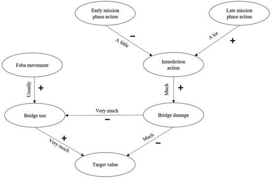
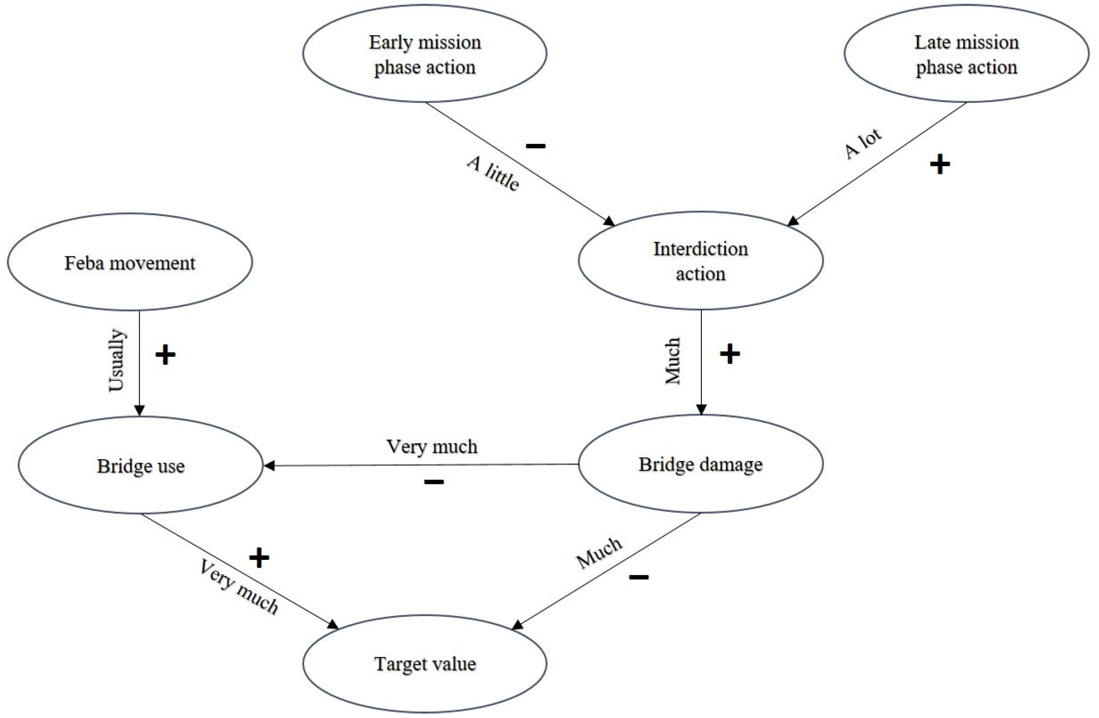
Kosko was the first to label arcs in a causal relation with fuzzy quantifiers. In [12], he includes a FCM (see Figure 1), illustrating causal relationships affecting a bridge as a tactical target in military science, exemplifying that if ‘interdiction action’ increases, ‘bridge damage’ also increases significantly, or that if ‘bridge damage’ increases, ‘bridge use’ decreases significantly.

Figure 1. Kosko’s causal map regarding bridge’s tactical target.

Kosko’s approach to fuzzy causality representation involves identifying nodes labeled by fuzzy concepts (including quantity or non-quantity fuzzy sets and fuzzy modifiers), and arcs weighted by fuzzy quantifiers. Although valuable, examples from real scenarios such as the one previously mentioned should be extended to other domains. This extension will permit proper testing as to what extent the usual expressions of causality are formulated using vague language.

To represent information, traditional graph theory metrics, such as PageRank or standard Betweenness Centrality, often fail to capture the nuances of causal dynamics. While PageRank identifies importance based on link frequency and Betweenness highlights nodes that lie on many paths, our model provides a more realistic weighting of causal intensity between nodes by incorporating negative weights, which aligns more closely with real-world interpretations. Consequently, we are able to calculate the specific strength of each causal path within the system, as a product of causal weights, allowing for the identification of the most potent causal chain rather than just the shortest path or the one with more links.

Taking as initial point the research by López et al. [18], which established methods for determining the causal intensity of various paths between nodes, this paper introduces a novel application of weighted causal graphs: the identification of new, causality-driven centrality measures. These metrics are designed to quantify vertex importance by analyzing the structural influence of a node, such as the cumulative strength of the paths originating from it. By utilizing a graph weighted through causal scores, we can adapt these values to highlight the most influential vertices and, consequently, predict the most potent sequence of effects triggered by a specific cause.

In Section 2, we detail these newly developed centrality measures applied to a causal graph, providing a comprehensive explanation of their mathematical foundations alongside a practical case study to illustrate their use. In addition to this, as the principal novelty of this work, we deal with negative weights in the causal graphs to model more realistic cases, and we systematize the process with an algorithm that calculates the proposed centrality measures. The choice of negative weights in some of the edges of a causal graph represents an advance with respect to previous works by the authors, since it models cases in which a vertex causes a negative effect on another one.

2. Weighted Centrality Measures

In this paper, we propose a modification of the centrality measures for vertices in causal graphs introduced in [18], by incorporating the weights of their incoming edges. This leads to the concept of a dynamic graph, where edge weights are not fixed but are instead computed based on their degree of causality. As a result, centrality is evaluated from a causal perspective.

To expand the scope of the measures defined in [18], we will allow negative weights to represent the idea of a concept that causes a negative effect (the opposite effect) on another concept.

With these premises, we establish the following definitions (see [18]):

Definition 1.

We define a causal graph associated with a set of concepts as a weighted, directed graph G = (V, E), where the vertices of V represent the selected concepts and $\left(a, b\right)\in E$ exists if vertex a directly causes the effect on vertex b (without any intermediate vertex). The weight of an edge (a, b), denoted as w(a, b), is a number in the interval $\left[-1, 1\right]$ indicating the degree to which vertex a directly causes the effect on vertex b for positive weights and the degree on which the vertex a directly causes the opposite effect on vertex b for negative weights.

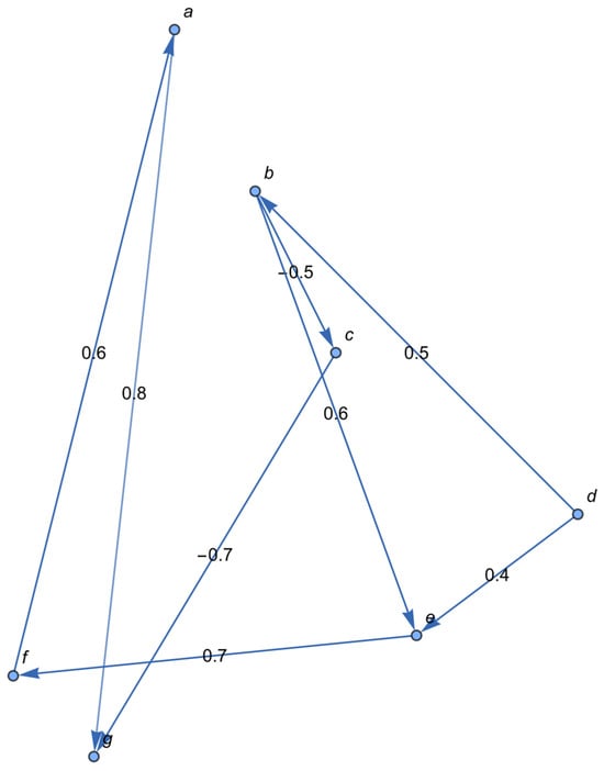
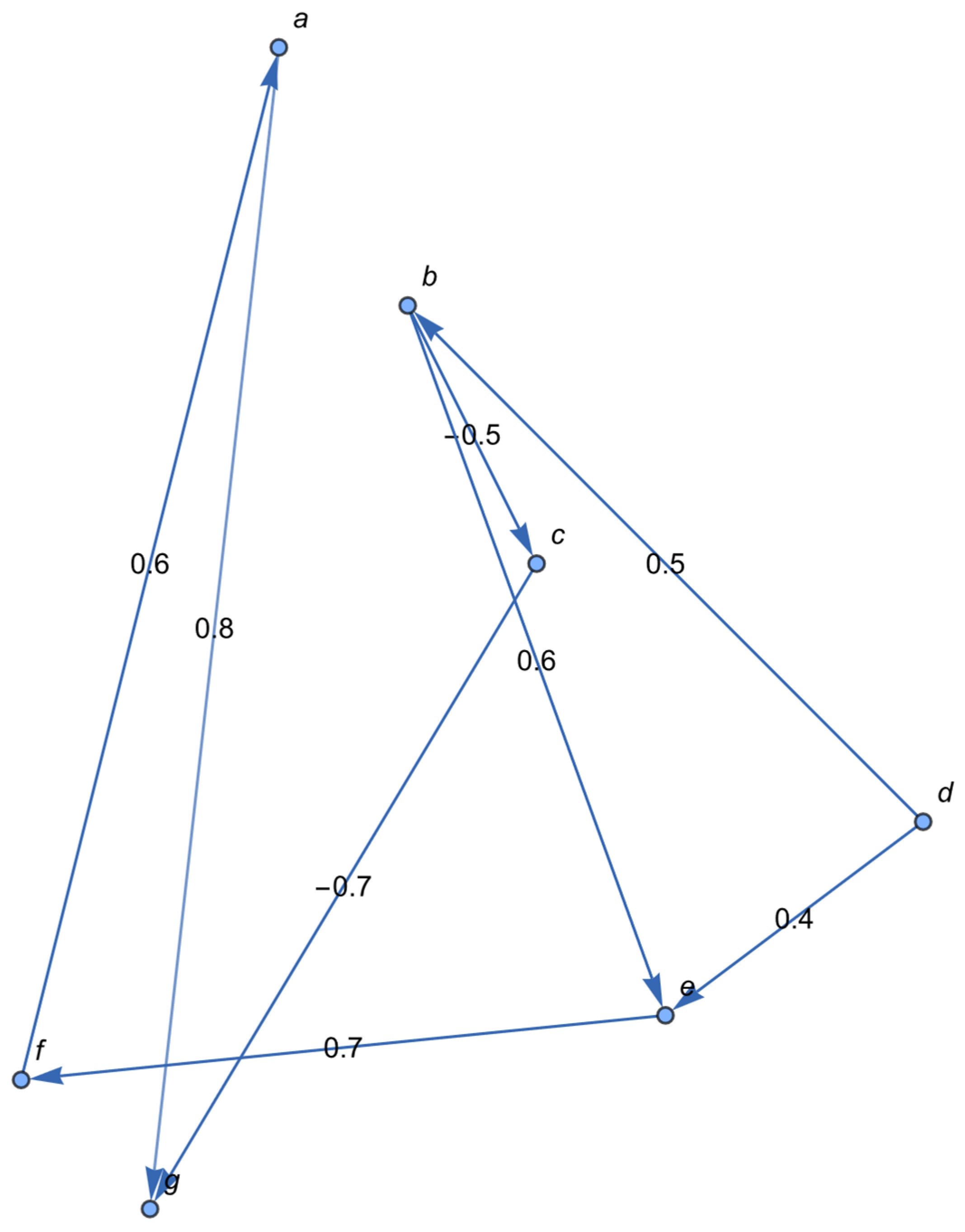
As an example, for the graph in Figure 2, if the vertex b represents sleep quality, the vertex c represents a high level of stress and the vertex e represents mental health; $w\left(b, e\right)=0.6$ indicates that sleep quality causes mental health at a degree of $0.6$, and $w\left(b, c\right)=-0.5$ indicates that sleep quality causes a low level of stress at a degree of $0.5$.

Figure 2. Causal graph G related to the example.

Remark 1.

If the causal graph G has edges with negative weights, then we can associate a new graph $G^{\prime }$ to G by duplicating the end vertices of the edges with negative weights, associating the opposite concepts to the duplicated vertices and giving the opposite weights to the corresponding edges. For example, due to the negative weight $w\left(b, c\right)=-0.5$, the associated graph will have a vertex $c^{\prime }$ that represents a low level of stress and an edge $\left(b, c^{\prime }\right)$ with $w\left(b, c^{\prime }\right)=0.5$. The associated graph will not have the edge $\left(b, c\right)$. This allows us to apply the techniques of [18].

Remark 2.

In this section we will assume that the causal graph G has n vertices with $n\ge 2$ and that it is an acyclic graph (a cycle would mean that a vertex indirectly causes itself, which does not make sense in a graph intended to model causality).

Definition 2.

Given a causal graph with vertices set $V=\left\{v_1, \dots , v_n\right\}$, its weighting matrix is $M={\left(a_{ij}\right)}_{n\times n}$, with: 

$$a_{ij}=\left\{\begin{array}{l}w\left(v_i, v_j\right) \mathrm{if} \left(v_i, v_j\right)\in E\\ 0 \mathrm{if} \left(v_i, v_j\right)\notin E\end{array}\right.$$

Definition 3.

Given a causal graph with set of vertices, $V=\left\{v_1, \dots , v_n\right\}$, we define the matrix $A={\left(a_{ij}\right)}_{n\times n}$, where: 

$$a_{ij}=\left\{\begin{array}{l}w\left(v_i, v_j\right) v_j \mathrm{if} \left(v_i, v_j\right)\in E\\ 0 \mathrm{if} \left(v_i, v_j\right)\notin E\end{array}\right.$$

Definition 4.

Given a causal graph with n vertices, $G=\left(V=\left\{v_1, \dots , v_n\right\}, E\right)$, we define recursively the matrix  $A_k$,  $k=1, \dots , n-1$ as:

$A_1={\left(a_{ij}\right)}_{n\times n}$, with  $a_{ij}=\left\{\begin{array}{l}w\left(v_i v_j\right) v_i v_j \mathrm{if} \left(v_i, v_j\right)\in E\\ 0 \mathrm{if} \left(v_i, v_j\right)\notin E\end{array}\right.$,  $A_k=A_{k-1} A$,  $k=2, \dots , n-1$.

The (symbolic) product of matrices is calculated without commuting factors.

Definition 5.

Given a causal graph of n vertices, the weighted out-degree of a vertex is the sum of all weights that originate from the vertex, and the weighted in-degree of a vertex is the sum of all the weights of the edges incident to the vertex.

Definition 6.

Given a causal graph of n vertices, the weighted centrality in the out-degree of a vertex is the weighted out-degree of such vertex divided by n − 1, and the weighted centrality in the in-degree of a vertex is the weighted in-degree of such vertex divided by n − 1.

Remark 3.

To calculate the weighted centrality out-degree of a vertex i, we just have to calculate the sum of the elements of the row i of the weighting matrix divided by the order of such matrix minus 1.

Remark 4.

To calculate the weighted centrality in-degree of a vertex i, we just have to calculate the sum of the elements of the column i of the weighting matrix divided by the order of such matrix minus 1.

We have a clear interpretation of these measures: the higher the value of the weighted centrality out-degree of a vertex i, the greater direct influence of this vertex on its neighbors. In a similar way, a high value of the weighted centrality in-degree for a vertex means a high influence of the neighbors on this vertex. The factor in the denominator serves only to normalize.

Definition 7.

Given a causal graph of n vertices, the weighted proximity centrality for the out-degree of a vertex is the sum of the degrees of all causal paths going from that vertex to the rest, divided by n, where the degree of a path is the product of the weights of the edges contained in the path, and a causal path is a path in a causal graph.

Definition 8.

Given a causal graph of n vertices, the weighted proximity centrality for the in-degree of a vertex v is the sum of the degrees of all causal paths going from all vertices to v, divided by n.

Remark 5.

To calculate the weighted proximity centrality out-degree of a vertex i, we just have to calculate the sum of the coefficients of the element (i, j) of the matrix $A_1+\dots +A_{n-1}$ and add these sums from j = 1 to n, dividing the result by n.

Remark 6.

To calculate the weighted proximity centrality in-degree of a vertex j, we just have to calculate the sum of the coefficients of the element (i, j) of the matrix $A_1+\dots +A_{n-1}$ and add these sums from i = 1 to n, dividing the result by n.

We can motivate these definitions in the following way: a high value of the weighted proximity centrality out-degree for a vertex indicates a high influence of this vertex on the rest of the vertices, taking into account the direct influence (direct edge) and the indirect influence (through intermediate vertices). Reciprocally, a high value of the weighted proximity centrality in-degree points out to a vertex that is highly influenced by the others, either in a direct or an indirect way.

In all cases we are looking for the vertex or vertices with the highest centrality measure.

Thus, we are going to establish an algorithm to calculate the weighted proximity centrality for the output degree of a vertex $v_i$. A similar algorithm would calculate the weighted proximity centrality for the in-degree of a vertex $v_i$, changing rows to columns.

Remark 7.

Steps 1–3 calculate the matrices $A_k$, $k=1, \dots , n-1$. Step 4 calculates the matrix $A_1+\dots +A_{n-1}$. Step 5 calculates the weighted proximity centrality for the output degree of the vertex $v_i$.

Remark 8.

Since the algorithm involves sums and products of n matrices of order n, it has a polynomial complexity.

Therefore, we are checking that the algorithm is correct and gives the desired centralities. We need a previous result:

Lemma 1.

The element $\left(i, j\right)$ of $A_k$ gives the paths from $v_i$ to $v_j$ of length k with their degrees for every $k=1, \dots , n-1$.

Proof. 

We prove this by induction on k. For $k=1$, we have two cases:

(1) If the element $\left(i, j\right)$ of $A_k$ is zero, then there is no direct path from $v_i$ to $v_j$.

(2) If the element $\left(i, j\right)$ of $A_k$ is $w\left(v_i v_j\right) v_i v_j$, then we have the edge $\left(v_i, v_j\right)$ in G, with weight $w\left(v_i v_j\right)$, so we have the path of length 1 $v_i-v_j$, with the degree $w\left(v_i v_j\right)$, as desired.

Assume that the result is true for $k-1$, so the element $\left(i, j\right)$ of $A_{k-1}$ gives the paths from $v_i$ to $v_j$ of length $k-1$ with their degrees.

Now, to obtain the element $\left(i, j\right)$ of $A_k$, we have to multiply the element $\left(i, s\right)$ of $A_{k-1}$ with the element $\left(s, j\right)$ of $A$ and add the results for $s=1, \dots , n$. We have three cases:

(1) If the element $\left(i, s\right)$ of $A_{k-1}$ is 0, then there are no paths in the graph from $v_i$ to $v_s$ of length $k-1$, so there are no paths in the graph from $v_i$ to $v_j$ of length $k$ containing $v_s$ as the penultimate vertex. Consequently, the product is 0.

(2) If the element $\left(s, j\right)$ of $A$ is 0, then there is no edge $\left(v_s, v_j\right)$ in the graph, so there are no paths in the graph from $v_i$ to $v_j$ of length $k$ containing $v_s$ as the penultimate vertex. Consequently, the product is 0.

(3) If the element $\left(i, s\right)$ of $A_{k-1}$ and the element $\left(s, j\right)$ of $A$ are nonzero, then the element $\left(i, s\right)$ of $A_{k-1}$ gives all the paths from $v_i$ to $v_s$ of length $k-1$ by the induction hypothesis. Then, the product of the two elements adds the edge $\left(v_s, v_j\right)$ at the end of the paths, so it gives all the paths from $v_i$ to $v_j$ of length $k$ containing $v_s$ as the penultimate vertex. If we add these products for $s=1, \dots , n$, we obtain all the paths from $v_i$ to $v_j$ of length $k$.

On the other hand, the coefficients in the element $\left(i, s\right)$ of $A_{k-1}$ are the degrees of the corresponding paths from $v_i$ to $v_s$ of length $k-1$ by the induction hypothesis. These degrees are the products of the labels of the edges in the path according to Definition 7. Therefore, the product with the coefficient in the element $\left(s, j\right)$ of $A$ yields the product of the weights of the edges in the path from $v_i$ to $v_j$ of length $k$ (the degree of the path), as desired. □

Proposition 1.

Let G be a causal graph and $v_i$ a vertex of G. Algorithm 1 gives the weighted proximity centrality for the output degree of  $v_i$.

Algorithm 1: Weighted proximity centrality for the output degree

Input: a causal graph G with n vertices given by its weighting matrix M.   Output: the weighted proximity centrality for the out-degree of a given vertex $v_i$.   Step 1: define k = 1.   Step 2: compute the product $A_k A$, where matrix $A$ is defined in Definition 3. Store the result as $A_{k+1}$ according to Definition 4.   Step 3: redefine $k=k+1$. If $k<n-1$, then return to step 2. If $k=n-1$, then go to step 4.   Step 4: Add the stored matrices $A_k$ for $k=1, \dots , n-1$.   Step 5: Add the coefficients of the elements of the row i of the matrix obtained in step 4. Divide the result by n.

Proof. 

The element $\left(i, j\right)$ of $A_k$ gives the paths from $v_i$ to $v_j$ of length k with their degrees by Lemma 1. The matrices $A_k$, $k=1, \dots , n-1$ are calculated and stored in the steps 1–3 of the algorithm when $k=n-1$. Now, the element $\left(i, j\right)$ of $A_1+\dots +A_{n-1}$ gives the paths from $v_i$ to $v_j$ of length $\le n-1$. Since G is acyclic, these are all the paths from $v_i$ to $v_j$. The matrix $A_1+\dots +A_{n-1}$ is calculated in step 4 of the algorithm. □

Consequently, the sum of the elements of the row i of $A_1+\dots +A_{n-1}$ gives all the paths from $v_i$ to the rest of the vertices with their degrees, so the sum of the coefficients of the elements of the row i gives the total degree of said paths. By Definition 7, dividing by n, we obtain the weighted proximity centrality of the output degree of $v_i$. This is done by step 5 of the algorithm.

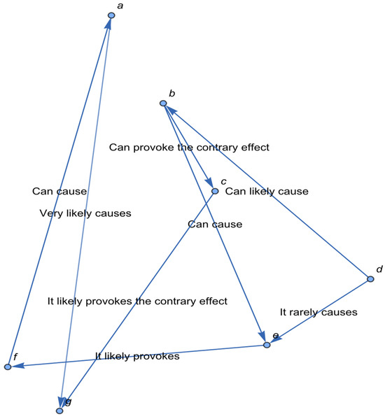
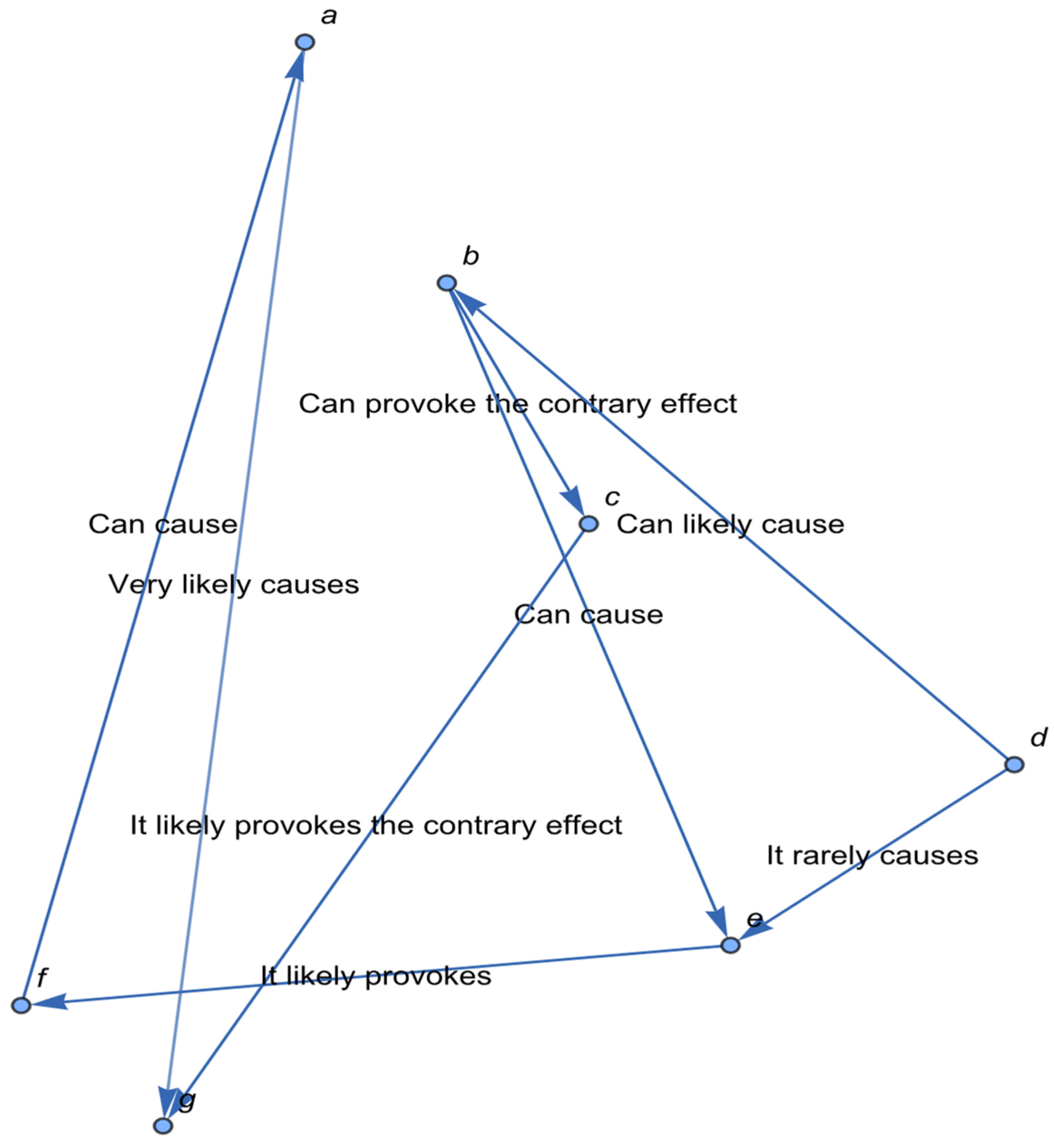
With these definitions and results, we propose a practical example based on Kosko’s causal map in Figure 3 and calculate the weighted centrality of its vertices. The map represents the causal linkages involved in a student’s time-planning problem.

Figure 3. Kosko’s causal map of student time planning.

We have seven vertices, a, …, g. The concepts behind the vertices are shown in Table 1.

Table 1. The vertices in the example.

Vertex	Concept Represented by the Vertex
a	Hours of study
b	Sleep quality
c	High level of stress
d	Diet
e	Mental health
f	Motivation
g	Good academic results

We also have the following edges and weights: $\left(a, g\right)$, $\left(b, c\right)$, $\left(c, e\right)$, $\left(c, g\right)$, $\left(d, b\right)$, $\left(d, e\right)$, $\left(e, f\right)$,

$w\left(a, g\right)=0.8$, $w\left(b, e\right)=0.6$, $w\left(b, c\right)=-0.5$, $w\left(c, g\right)=-0.7$,

$w\left(d, b\right)=0.5$, $w\left(d, e\right)=0.4$, $w\left(e, f\right)=0.7$, $w\left(f, a\right)=0.6$

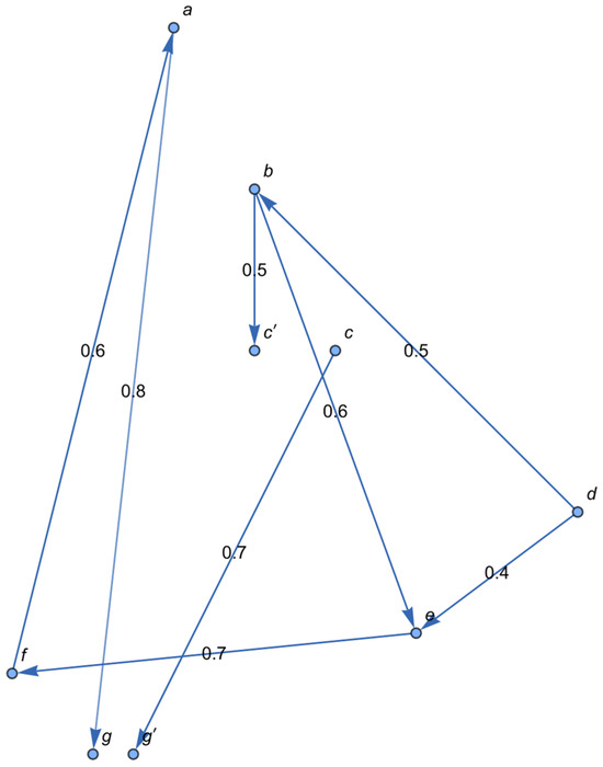
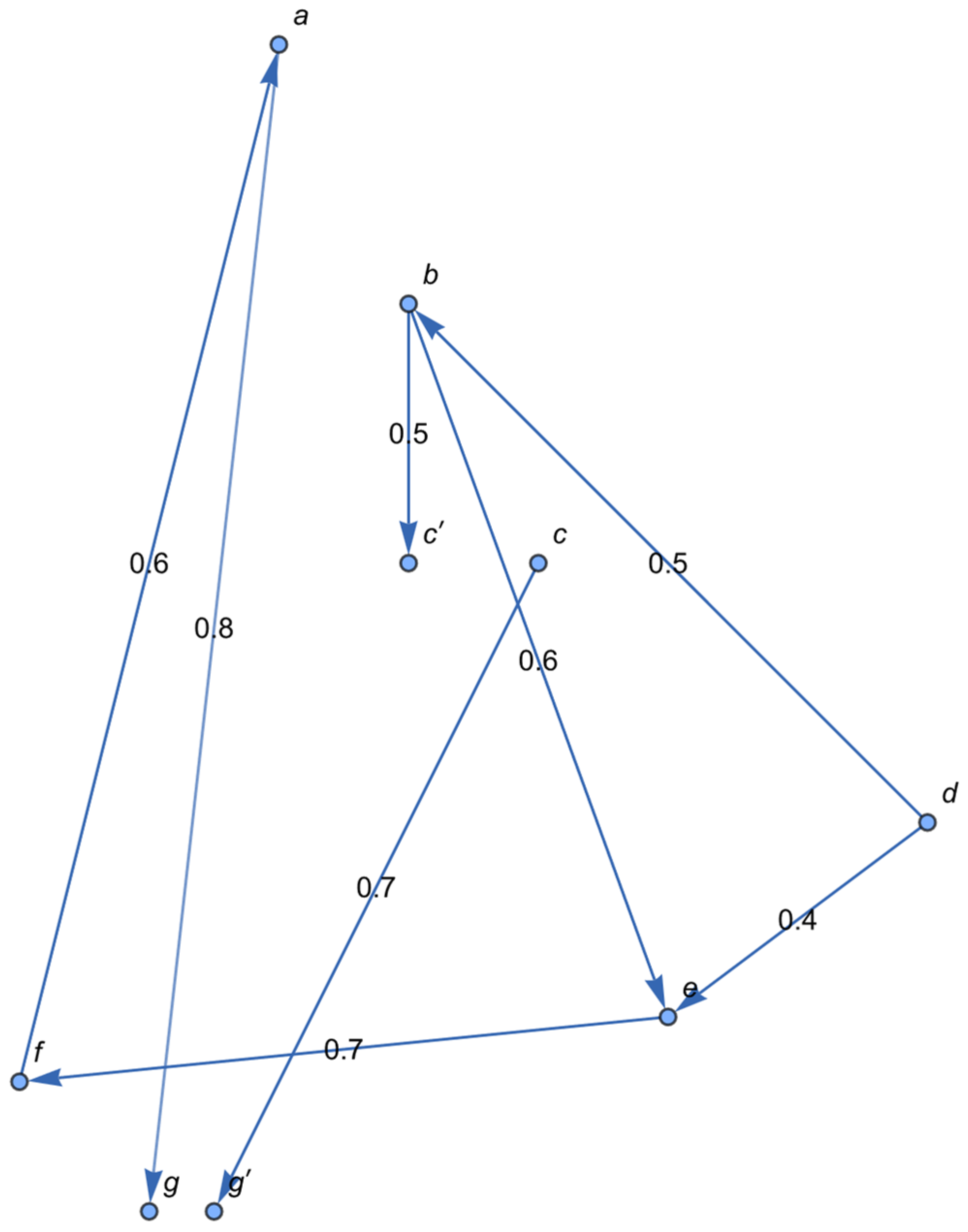
To avoid negative weights, we add a vertex $c^{\prime }$ associated to the concept “low level of stress”, and a vertex $g^{\prime }$ associated to the concept “bad academic results”, establishing the edges $\left(b, c^{\prime }\right)$, with weight $0.5$ and $\left(c, g^{\prime }\right)$, with weight $0.7$. We also remove the edges $\left(b, c\right)$, $\left(c, g\right)$ to obtain the associated graph $G^{\prime }$ that we are going to use (see Figure 4).

Figure 4. The associated graph $G^{\prime }$ related to the example.

Therefore, the weighting matrix of $G^{\prime }$ is (with the vertices arranged as a, …, g, $c^{\prime }$, $g^{\prime }$):

$$M=\left(\begin{array}{ccccccccc}0& 0& 0& 0& 0& 0& 0.8& 0& 0\\ 0& 0& 0& 0& 0.6& 0& 0& 0.5& 0\\ 0& 0& 0& 0& 0& 0& 0& 0& 0.7\\ 0& 0.5& 0& 0& 0.4& 0& 0& 0& 0\\ 0& 0& 0& 0& 0& 0.7& 0& 0& 0\\ 0.6& 0& 0& 0& 0& 0& 0& 0& 0\\ 0& 0& 0& 0& 0& 0& 0& 0& 0\\ 0& 0& 0& 0& 0& 0& 0& 0& 0\\ 0& 0& 0& 0& 0& 0& 0& 0& 0\end{array}\right)$$

If we apply the first observation of Definition 6, we obtain the following weighted centralities for the out-degree:

a: ${\displaystyle \frac{1}{8}} 0.8=0.1$, b: ${\displaystyle \frac{1}{8}} \left(0.6+0.5\right)=0.1375$, c: ${\displaystyle \frac{1}{8}} 0.7=0.0875$, d: ${\displaystyle \frac{1}{8}} \left(0.5+0.4\right)=0.1125$, e: ${\displaystyle \frac{1}{8}} 0.7=0.0875$, f: ${\displaystyle \frac{1}{8}} 0.6=0.075$, g: 0, $c^{\prime }$: 0, $g^{\prime }$: 0.

Therefore, b (sleep quality) is the vertex with the highest weighted output centrality degree.

Applying Remark 2 of Definition 6, we obtain the following weighted centralities for the in-degree:

a: ${\displaystyle \frac{1}{8}} 0.6=0.075$, b: 0, c: 0, d: ${\displaystyle \frac{1}{8}} 0.5=0.0625$, e: ${\displaystyle \frac{1}{8}} \left(0.6+0.4\right)=0.125$, f: ${\displaystyle \frac{1}{8}} 0.7=0.0875$, g: ${\displaystyle \frac{1}{8}} 0.8=0.1$, $c^{\prime }$: ${\displaystyle \frac{1}{8}} 0.5=0.0625$, $g^{\prime }$: ${\displaystyle \frac{1}{8}} 0.7=0.0875$.

Therefore, e (mental health) is the vertex with highest weighted input centrality degree.

The matrix $A_1+\dots +A_{n-1}$ of this graph is:

$$\left(\begin{array}{ccccccccc}0& 0& 0& 0& 0& 0& 0.8ag& 0& 0\\ 0.252befa& 0& 0& 0& 0.6be& 0.42bef& 0.2016befag& 0.5b{c}^{\prime }& 0\\ 0& 0& 0& 0& 0& 0& 0& 0& 0.7c{g}^{\prime }\\ 0.168defa+0.126debfa& 0.5db& 0& 0& 0.4de+0.3dbe& 0.28def+0.21debf& 0.1344defag+0.1008debfag& 0.25db{c}^{\prime }& 0\\ 0.42efa& 0& 0& 0& 0& 0.7ef& 0.336efag& 0& 0\\ 0.6fa& 0& 0& 0& 0& 0& 0.48fag& 0& 0\\ 0& 0& 0& 0& 0& 0& 0& 0& 0\\ 0& 0& 0& 0& 0& 0& 0& 0& 0\\ 0& 0& 0& 0& 0& 0& 0& 0& 0\end{array}\right)$$

Applying observation 1 of Definitions 7 and 8 (Algorithm 1), we obtain the following weighted proximity centralities for the out-degree (rounded to the second decimal):

a: ${\displaystyle \frac{1}{9}} 0.8=0.09$, b: ${\displaystyle \frac{1}{9}} \left(0.252+0.6+0.42+0.2016+0.5\right)=0.22$, c: ${\displaystyle \frac{1}{9}} 0.7=0.08$, d: ${\displaystyle \frac{1}{9}} \left(0.168+0.126+0.5+0.4+0.3+0.28+0.21+0.1344+0.1008+0.25\right)=0.27$, e: ${\displaystyle \frac{1}{9}} \left(0.42+0.7+0.336\right)=0.16$, f: ${\displaystyle \frac{1}{9}} \left(0.6+0.48\right)=0.12$, g, $c^{\prime }$ and $g^{\prime }$: 0.

Therefore, d (diet) is the vertex with the highest weighted proximity centrality for the out-degree.

The paths from d to the rest of the vertices and their weights are contained in the fourth row of $A_1+\dots +A_{n-1}$. We summarize them in the table below (Table 2).

Table 2. Paths from d to the rest of vertices and their weights.

Path	Weight
defa	0.168
debfa	0.126
db	0.5
de	0.4
dbe	0.3
def	0.28
debf	0.21
defag	0.1344
debfag	0.1008
dbc′	0.25

Applying observation 2 of Definitions 7 and 8, we obtain the following weighted proximity centralities for the in-degree (rounded to the second decimal):

a: ${\displaystyle \frac{1}{9}} \left(0.252+0.168+0.126+0.42+0.6\right)=0.17$, b: ${\displaystyle \frac{1}{9}} 0.5=0.06$, c and d: 0, e: ${\displaystyle \frac{1}{9}} \left(0.6+0.4+0.3\right)=0.14$, f: ${\displaystyle \frac{1}{9}} \left(0.42+0.28+0.21+0.7\right)=0.18$, g: ${\displaystyle \frac{1}{9}} \left(0.8+0.2016+0.1344+0.1008+0.336+0.48\right)=0.23$, $c^{\prime }$: ${\displaystyle \frac{1}{9}} \left(0.5+0.25\right)=0.08$, $g^{\prime }$: ${\displaystyle \frac{1}{9}} 0.7=0.08$.

Therefore, g (good academic results) is the vertex with the highest weighted proximity centrality in the in-degree.

The paths from the other vertices to g and their weights are contained in the seventh column of $A_1+\dots +A_{n-1}$. We summarize them in the table below (Table 3).

Table 3. Paths from the remaining vertices to g and their weights.

Path	Weight
ag	0.8
befag	0.2016
defag	0.1344
debfag	0.1008
efag	0.336
fag	0.48

Finally, we summarize the procedure carried out in this section.

-

From Kosko’s causal map, define a causal graph G with positive weights for the positive effects and negative weights for the negative ones.

-

If G has edges with negative weights, associate a new graph $G^{\prime }$ to G by duplicating vertices, inserting new edges and removing the old edges with negative weights. This new graph $G^{\prime }$ can be processed since all its edges have positive weights.

-

Calculate the centrality measures of the vertices by means of Algorithm 1. Identify the most relevant vertices according to these measures.

-

Find the causal paths from the relevant vertices to the remaining ones.

3. Conclusions

Causal graphs are used as knowledge structures in both scientific research and computational modeling. However, a persistent challenge in these representations is determining the optimal or ‘most’ causal path between two nodes [19], together with the central nodes.

In this paper we have improved several aspects regarding the representation and weighting of causal graphs. First, our model successfully identifies key central concepts based on their causal influence; as shown in the student planning example, the framework identifies “Diet” as a significant causal driver and “Academic Results” as a primary cumulative effect.

The main contribution of the paper is the consideration of negative weights on the edges of the causal graphs to model the fact that one concept may produce a contrary effect on another. With this new perspective, in order to process and manage the causal graph, we associate it with a new graph with positive weights, which allows us to generate an algorithm that identifies the key central concepts according to the centrality measures defined. We have also proven the correctness and efficiency of the algorithm.

Moreover, we have demonstrated that this model evaluates the “most causal path” between concepts, allowing for a formal mathematical definition of a route from origin to destination that accurately reflects the intensity of the causal influence distributed throughout the network.

Thus, by moving beyond qualitative weightings such as “always” or “sometimes,” we provide a framework that ranks nodes according to their empirical causal importance. This transition from static connectivity to dynamic causal weighting enables researchers to predict the strongest set of effects triggered by a specific cause. The resulting causal ranking provides a superior basis for complex applications compared to static graphs. Specifically, this framework improves accuracy in fields such as automatic text summarization [20] and question-answering systems [21] by prioritizing the nodes with the highest causal relevance.

References

- Bunge, M. Causality: The Place of the Causal Principle in Modern Science; Harvard University Press: Cambridge, UK, 1959. [Google Scholar]
- Puente, C. Causality in science. Pensam. Matemático 2011, 1, 12. [Google Scholar]
- Hume, D. A Treatise of Human Nature; Norton, D.F., Norton, U.J., Eds.; Oxford University Press: Oxford, UK, 2000. [Google Scholar]
- Kant, I. Critique of Pure Reason, 2nd ed.; Smith, N.K., Translator; Macmillan: London, UK, 1929. [Google Scholar]
- Mill, J.S. A System of Logic, Ratiocinative and Inductive: Being a Connected View of the Principles of Evidence and the Methods of Scientific Investigation, 8th ed.; Harper & Brothers: New York, NY, USA, 1874. [Google Scholar]
- Mach, E. Knowledge and Error; Reidel: Dordrecht, The Netherlands, 1976. [Google Scholar]
- Davidson, D. Essays on Actions and Events; Clarendom Press: Oxford, UK, 1980. [Google Scholar]
- Mazlack, L.J. Imperfect Causality. Fundam. Inform. 2004, 59, 191–201. [Google Scholar]
- Pearl, J. Causality, Models, Reasoning, and Inference; Cambridge University Press: Cambridge, UK, 2000. [Google Scholar]
- Spirtes, P.; Glymour, C.; Scheines, R. Causation, Prediction and Search, 2nd ed.; MIT Press: Cambridge, MA, USA, 2000. [Google Scholar]
- Sobrino, A.; Puente, C.; Olivas, J.A. Extracting answers from causal mechanisms in a medical document. Neurocomputing 2014, 135, 53–60. [Google Scholar] [CrossRef] [Scilit]
- Kosko, B. Fuzzy Cognitive Maps. Int. J. Man-Mach. Stud. 1986, 24, 65–75. [Google Scholar] [CrossRef] [Scilit]
- Axelrod, R. The Structure of Decision: The Cognitive Maps of Political Elites; Princeton University Press: Princeton, NJ, USA, 1976. [Google Scholar]
- Aguilar, J. A survey about Fuzzy Cognitive Maps Papers (Invited Paper). Int. J. Comput. Cogn. 2005, 3, 27–33. [Google Scholar]
- Carvalho, J.P.; Tomé, J.A.B. Fuzzy Mechanisms for Causal Relations. In Proceedings of the Eighth International Fuzzy Systems Association World Congress, IFSA’99, Taipei, Taiwan, 17–20 August 1999. [Google Scholar]
- Benferhat, S.; Bonnefon, J.F.; Chassy, P.; Da Silva Neves, R.; Dubois, D.; Dupin de Saint-Cyr, F.; Kayser, D.; Nouioua, F.; Nouioua-Boutouhami, S.; Prade, H.; et al. A Comparative Study of Six Formal Models of Causal Ascription. In SUM 2008; LNAI; Greco, S., Lukasiewicz, T., Eds.; Springer: Berlin/Heidelberg, Germany, 2008; Volume 5291, pp. 47–62. [Google Scholar]
- Boutouhami, S.; Mokhtari, A. Possibilistic Explanation. Int. J. Comput. Sci. Appl. 2006, 3, 57–73. [Google Scholar]
- Puente Águeda, C.; López González, M.D.; Rodrigo Hitos, J.; Olivas Varela, J.A. Weighted Graphs to Model Causality. In Proceedings of the ICAI 2017 (International Conference on Artificial Intelligence), Las Vegas, NV, USA, 17–20 July 2017; pp. 297–301. [Google Scholar]
- Puente, C.; Sobrino, A.; Olivas, J.A.; Merlo, R. Extraction, analysis and representation of imperfect conditional and causal sentences by means of a semi-automatic process. In Proceedings of the Fuzzy Systems (FUZZ), 2010 IEEE International Conference, Barcelona, Spain, 18–23 July 2010; pp. 1–8. [Google Scholar]
- Puente, C.; Sobrino, A.; Olivas, J.A.; Garrido, E. Summarizing information by means of causal sentences through causal graphs. J. Appl. Log. 2017, 24, 3–14. [Google Scholar] [CrossRef] [Scilit]
- Puente, C.; Sobrino, A.; Olivas, J.Á. Extraction of conditional and causal sentences from queries to provide a flexible answer. In International Conference on Flexible Query Answering Systems; Springer: Berlin/Heidelberg, Germany, 2009; pp. 477–487. [Google Scholar]
Disclaimer/Publisher’s Note: The statements, opinions and data contained in all publications are solely those of the individual author(s) and contributor(s) and not of MDPI and/or the editor(s). MDPI and/or the editor(s) disclaim responsibility for any injury to people or property resulting from any ideas, methods, instructions or products referred to in the content. |
© 2026 by the authors. Licensee MDPI, Basel, Switzerland. This article is an open access article distributed under the terms and conditions of the Creative Commons Attribution (CC BY) license.