A Dependent Bivariate Burr XII Inverse Weibull Model: Application to Diabetic Retinopathy and Dependent Competing Risks Data

Abstract

This paper introduces a novel bivariate distribution, referred to as the Bivariate Burr XII Inverse Weibull (BBXII-IW) distribution, constructed via the Marshall–Olkin approach from the univariate Burr XII Inverse Weibull (BXII-IW) distribution. The proposed BBXII-IW model provides a flexible framework for modeling dependent bivariate data, including competing risk scenarios. The key statistical properties of the distribution are derived, and parameter estimation is conducted using the maximum likelihood method. The model’s performance is evaluated using two types of real-world datasets: (1) bivariate data and (2) dependent competing risk data related to diabetic retinopathy. The results demonstrate that the BBXII-IW distribution offers an improved fit compared to existing models, highlighting its flexibility and practical relevance in modeling complex dependent structures.

1. Introduction

In reliability and survival analysis, the failure of a unit is often attributed to multiple competing factors throughout its lifecycle, described as a competing risk model (see Crowder [1]). Typically, competing risk data consist of failure times and indicators identifying the specific cause of failure. Inference in competing risk models has been widely studied under the assumption that the causes of failure operate independently. Notable contributions include the works of Ren and Gui [2], Wang et al. [3], and Mahto et al. [4], among others. However, in real-world scenarios, this independence assumption often fails to hold due to complex interdependencies within and surrounding the unit.

For example, in the case of colon cancer, the two primary causes of failure—cancer recurrence and death—are interdependent, influencing one another. Similarly, in a two-engine aircraft, the failure of one engine places additional stress on the other, thereby increasing its likelihood of failure. These interdependencies highlight the need for models that explicitly account for dependent causes of failure. Common approaches for addressing such dependencies include multivariate lifetime distributions (Crowder [1]), copula models (Nelsen [5]), and frailty models (Duchateau and Janssen [6]).

Theoretical and empirical studies have extensively explored competing risk models with dependent failure causes. Notable contributions include the works of Wang et al. [7], Gorfine and Hsu [8], Lo and Wilke [9], Fan et al. [10], and Xu et al. [11,12].

The Marshall–Olkin (MO)-type distribution is extensively used for modeling the failure of correlated paired data, particularly in reliability and survival analysis. A variety of bivariate distributions have been derived from the Marshall–Olkin framework. Marshall and Olkin [13] initially introduced the bivariate exponential distribution based on this approach, laying the groundwork for significant advancements in the field. Kotz et al. [14] provided a comprehensive analysis of bivariate models derived from the Marshall–Olkin methodology.

In recent years, extensions of MO-type distributions have proliferated. For example, Sarhan and Balakrishnan [15] proposed the Sarhan–Balakrishnan bivariate distribution. Sarhan et al. [16] proposed the bivariate generalized linear failure rate (BGLFR) distribution, and Sarhan et al. [17] introduced the bivariate Chen distribution (BCD). Bai et al. [18] proposed a bivariate Weibull distribution, while Bakouch et al. [19] introduced the bivariate Kumaraswamy-exponential distribution. Kilany and El-Qareb [20] examined bivariate failure time models using the extended Chen distribution, and Manshi et al. [21] developed the bivariate modified Weibull extension (BMWE) distribution. Further innovations continue to enrich this class of distributions. Sarhan et al. [22] very recently proposed the bivariate exponentiated generalized inverted exponential distribution (BEGIE) within the MO framework.

This paper uses the MO-type to introduce a novel bivariate distribution called the Bivariate Burr XII Inverse Weibull (BBXII-IW) distribution. This model is derived by extending the univariate Burr XII Inverse Weibull (BXII-IW) distribution, originally proposed by Shrahili [23], using the Marshall–Olkin methodology. The BBXII-IW distribution generalizes several established bivariate models and offers a new approach for capturing intricate dependencies in bivariate reliability data.

The main contributions of this paper are summarized as follows:

• Introduced a new five-parameter Bivariate Burr XII Inverse Weibull (BBXII-IW) distribution via the Marshall–Olkin approach.
• Derived key statistical properties, including joint and marginal PDFs, survival functions, and hazard functions.
• Established closed-form expressions for singular and continuous components of the joint distribution.
• Applied maximum likelihood estimation techniques for both bivariate and dependent competing risks data.
• Conducted simulation and real-data applications demonstrating superior performance over existing models (BEGIE, BVGE, and BGLFR).

The remainder of this paper is organized as follows. In Section 2, we provide the motivation for the proposed distribution. Section 3 reviews the univariate Burr XII Inverse Weibull (BXII-IW) distribution and its key properties. In Section 4, we introduce the new Bivariate Burr XII Inverse Weibull (BBXII-IW) distribution and derive its statistical properties, including joint and marginal functions. Section 5 presents the maximum likelihood estimation procedures for both bivariate and dependent competing risk data. A simulation study evaluating the performance of the estimators is given in Section 6. Section 7 provides applications to real-world datasets. Finally, Section 8 concludes this paper with a summary and discussion of potential future research directions.

2. Motivation

Modeling dependent lifetimes or failure times is of fundamental importance in reliability theory, survival analysis, and biomedical research, especially in scenarios involving competing risks or multicomponent systems. Traditional competing risk models often assume independence between failure causes, which can be unrealistic in many real-world applications. For instance, the recurrence of a disease and death may not be statistically independent, and failure of one component in a system (e.g., a twin-engine aircraft) may increase the stress on and risk of failure in the other.

In such settings, multivariate lifetime models that incorporate dependence structures are required to accurately capture system behavior. Among these, the Marshall–Olkin (MO) family of distributions has been extensively employed for modeling dependent risks and failure data due to its tractability and interpretability.

Additionally, there is a growing need for flexible lifetime models that can accommodate various shapes of hazard rate functions (increasing, decreasing, unimodal, etc.) and model heavy-tailed data effectively. The Burr XII Inverse Weibull (BXII-IW) distribution has demonstrated excellent performance in this regard for univariate data, offering superior fits in diverse domains such as medical data, environmental studies, and insurance claims.

This paper is motivated by the goal of combining the dependence structure of the Marshall–Olkin framework with the modeling flexibility of the BXII-IW distribution. Specifically, we propose a novel five-parameter bivariate distribution, referred to as the Bivariate Burr XII Inverse Weibull (BBXII-IW) distribution, which generalizes several known models and provides a comprehensive framework for analyzing dependent bivariate lifetime and competing risks data.

3. BXII-IW Distribution

Shrahili [23] introduced the Burr XII Inverse Weibull (BXII-IW) distribution, including three parameters. The three primary functions associated with the BXII-IW$(\gamma ,a,b)$ distribution are as follows. The probability density function (pdf) is as follows:

$$g(x;\gamma ,a,b)={\displaystyle \frac{ab\gamma x^{-\gamma -1}exp\left(-a{x}^{-\gamma }\right)}{{\left[1-exp\left(-x^{-\gamma }\right)\right]}^{a+1}}}{\left\{1+{\left[exp\left(x^{-\gamma }\right)-1\right]}^{-a}\right\}}^{-b-1},x\ge 0,\gamma ,a,b>0.$$

(1)

The survival function (sf) is as follows:

$$S_0(x;\gamma ,a,b)={\left\{1+{\left[exp\left(x^{-\gamma }\right)-1\right]}^{-a}\right\}}^{-b},x\ge 0,\gamma ,a,b>0.$$

(2)

The hazard rate function (hrf) is defined as

$$h(x;\gamma ,a,b)={\displaystyle \frac{ab\gamma x^{-\gamma -1}exp\left(-a{x}^{-\gamma }\right)}{{\left[1-exp\left(-x^{-\gamma }\right)\right]}^{a+1}}}{\left\{1+{\left[exp\left(x^{-\gamma }\right)-1\right]}^{-a}\right\}}^{-1},x\ge 0,\gamma ,a,b>0.$$

(3)

According to Shrahili [23], the BXII-IW distribution demonstrates remarkable flexibility in modeling diverse hazard rate behaviors, including increasing, decreasing, upside-down, or growing shapes. This versatility was a key motivation behind its development, enabling it to effectively accommodate a wide range of univariate lifetime datasets in survival and reliability analysis.

Using three univariate real datasets, the BXII-IW distribution has been shown to outperform several notable competing models, including the standard Inverse Weibull (IW), Weibull IW, Poisson BurrX IW, Exponentiated IW, Kumaraswamy IW, Transmuted IW, Generalized Marshall–Olkin Kumaraswamy IW, Marshall–Olkin IW, Beta IW, Marshall–Olkin Kumaraswamy IW, and Gamma Extended IW.

This model is applicable across a variety of fields, including extreme weather events like floods, maximum sizes of ecological populations, the magnitude of freak waves, significant insurance losses, equity risks, daily market risks, drug side effects, survival times, large wildfires, and repair data in reliability contexts.

The BXII-IW$(\gamma ,a,b)$ distribution also serves as a generalization of several well-known distributions, as detailed below:

• When $\gamma =2$, the BXII-IW model simplifies to the BrXII Inverse Rayleigh (BXII-IR) model (Yousof et al. [24]). The BXII-IR model is an extension of the Burr XII (BrXII) distribution that has gained attention for its versatility in modeling various types of data. It is useful in areas such as actuarial and survival analysis due to its ability to represent different behaviors in data, including heavy tails and skewness. The BXII-IR distribution generalizes the Burr XII distribution and incorporates features like inverse Rayleigh-like behavior, making it applicable to datasets with specific risk or reliability characteristics
• When $\gamma =1$, the BXII-IW model simplifies to the BXII Inverse Exponential (BXII-IE) model (Bhatti et al. [25]). The Burr XII Inverse Exponential (BXII-IE) distribution, as part of the Burr family of distributions, is a flexible statistical model with applications in various fields, including reliability, survival analysis, and actuarial science. Its importance stems from its ability to capture diverse hazard rate behaviors (e.g., increasing, decreasing, or constant rates) and model data with heavy tails, skewness, and other complex patterns.
• When $b=1$, the BXII-IW model reduces to the Log-Logistic Inverse Weibull (LogL-IW) model (Kumar and Nair [26]). The LogL-IW model is widely used in survival analysis, hydrology, and economics due to its flexibility in modeling unimodal and monotonic hazard functions. It can describe survival data with non-monotonic hazard rates and is applied in analyzing rainfall extremes and wealth distribution.
• When $a=1$, the BXII-IW model simplifies to the Lomax Inverse Weibull (LIW) model (Goual et al. [27]). The LIW distribution combines the Lomax and Inverse Weibull properties, making it particularly suitable for modeling survival and reliability data where long tails or heavy-tailed behaviors are observed. This distribution is often applied in fields like finance, insurance, and environmental studies to analyze extreme events, such as large insurance claims, catastrophic risks, or extreme environmental phenomena. Its versatility in hazard rate shapes further enhances its applicability in diverse real-world datasets.

4. BBXII-IW Distribution

Let $U_i$, $(i=1,2,3)$, be independent random variables following the BXII-IW$(\gamma ,a,b_j)$ distribution and define $X_j=min(U_j,U_3)$ for $j=1,2$. Then, the pair of random variables $(X_1,X_2)$ follows the Bivariate Burr XII Inverse Weibull (BBXII-IW) distribution with parameters $(\gamma ,a,b_1,b_2,b_3)$, where $\gamma ,a,b_1,b_2,b_3>0$.

In a reliability framework, this model can describe a system consisting of two components subject to three independent shock sources. A shock from the first source destroys only component 1, a shock from the second source destroys only component 2, and a shock from the third source destroys both components simultaneously. Let $U_i$ denote the time of a shock from source i, and the lifetimes of components 1 and 2, denoted by $X_1$ and $X_2$ can be expressed as $X_1=min(U_1,U_3)$ and $X_2=min(U_2,U_3)$, respectively. This representation models each unit as a series system influenced by shared and individual shock sources. Consequently, the random variables $(X_1$ and $X_2)$ are shown to follow the BBXII-IW distribution when the shock times are governed by BXII-IW distributions.

The key properties and implications of the BBXII-IW distribution are summarized in the following theorem, highlighting its joint probability density function, its joint survival function, and its marginal distributions.

Theorem 1.

Suppose $(X_1,X_2)\sim$ BBXII-IW$(\gamma ,a,b_1,b_2,b_3)$; then, we have the following:

1. 

The bivariate survival function of $(X_1,X_2)$ is

$$S(x_1,x_2)=\left\{\begin{array}{cc}{S}_0(x_1;\gamma ,a,b_1+b_3)S_0(x_2;\gamma ,a,b_2)\hfill & x_1\ge x_2>0,\hfill \\ S_0(x_1;\gamma ,a,b_1)S_0(x_2;\gamma ,a,b_2+b_3)\hfill & x_2>x_1>0,\hfill \end{array}\right.$$

(4)

2. 

The bivariate probability density function (pdf) of $(X_1,X_2)$ is

$$f(x_1,x_2)=\left\{\begin{array}{cc}{f}_1(x_1,x_2)=g(x_1;\gamma ,a,b_1+b_3)g(x_2;\gamma ,a,b_2)\hfill & x_1>x_2>0,\hfill \\ f_2(x_1,x_2)=g(x_1;\gamma ,a,b_1)g(x_2;\gamma ,a,b_2+b_3)\hfill & x_2>x_1>0,\hfill \\ f_0\left(x\right)={\displaystyle \frac{b_3}{b_1+b_2+b_3}}g(x;\gamma ,a,b_1+b_2+b_3)\hfill & x_1=x_2=x>0.\hfill \end{array}\right.$$

(5)

3. 

The marginal distribution of $X_j$ follows BXII-IW$(\gamma ,a,b_j+b_3)$, $j=1,2$,

where $S_0(x;\gamma ,a,b)$ and $g(x;\gamma ,a,b)$ are the survival and probability density functions, given in Equations (1) and (2), respectively.

Proof. 

• Using the basic definition of survival function $S(x_1,x_2)=P(X>x_1,X_2>x_2$, we obtain

  $$\begin{array}{ccc}\hfill S(x_1,x_2)& =& P(min(U_1,U_3)>x_1,min(U_2,U_3)>x_2)\hfill \\ & =& P(U_1>x_1,U_2>x_2,U_3>max(x_1,x_2))\hfill \\ & =& S_0(x_1;\gamma ,a,b_1)S_0(x_2;\gamma ,a,b_2)S_0(max(x_1,x_2);\gamma ,a,b_3)\hfill \end{array}$$

  (6)

  Substituting from (2) into (6), we obtain $S(x_1,x_2)$.
• Since the joint probability density function (pdf), $f(x_1,x_2)$ of $(X_1,X_2)$, exhibits singularity when $X_1=X_2$, the distinct components of the pdf, denoted as $f_1(x_1,x_2)$ and $f_2(x_1,x_2)$, on domains $x_1>x_2$ and $x_2>x_1$, respectively, can be derived. This is achieved by calculating the second partial derivatives of the survival function $S(x_1,x_2$, as expressed in (4), with respect to $x_1$ and $x_2$. The singular part $f_0\left(x\right)$, corresponding to the diagonal $X_1=X_2$, can be obtained by employing the normalization condition of probabilities:

  $${\int }_0^{\infty }{\int }_0^{x_1}{f}_1(x_1,x_2)d{x}_{2}d{x}_1+{\int }_0^{\infty }{\int }_0^{x_2}{f}_1(x_1,x_2)d{x}_{1}d{x}_2+{\int }_0^{\infty }{f}_0\left(x\right)dx=1$$

  This equation ensures that the total probability integrates to unity, accounting for the contributions from the non-singular regions $x_1>x_2$ and $x_2>x_1$ and the singular region $X_1=X_2$.
• The marginal distribution of $X_1$ can be obtained by getting the marginal survival function of $X_1$ as follows:

  $$\begin{array}{ccc}\hfill S_1\left(x_1\right)& =& P(X_1>x_1)=P(min(U_1,U_3)>x_1)=P(U_1>x_1)P(U_3>x_1)\hfill \\ & =& S_0(x_1;\gamma ,a,b_1)S_0(x_1;\gamma ,a,b_3)=S_0(x_1;\gamma ,a,b_1+b_3)\hfill \end{array}$$

  (7)

  That is, $X_1$ follows BXII-IW$(\gamma ,a,b_1+b_3)$. Similarly, we can show that $X_2$ follows BXII-IW$(\gamma ,a,b_2+b_3)$, which completes the proof of this part.

   □

By substituting (1) into (5), we can derive the explicit forms for $f_1$, $f_2$, and $f_0$ in the following expressions:

$$f_1(x_1,x_2)={\displaystyle \frac{(b_1+b_3)b_{2}a\gamma {\left(1+{\left(e^{x_1^{-\gamma }}-1\right)}^{-a}\right)}^{-b_1-b_3-1}{\left(1+{\left(e^{x_2^{-\gamma }}-1\right)}^{-a}\right)}^{-b_2-1}}{{\left(x_1{x}_2\right)}^{\gamma +1}\left(e^{x_1^{-\gamma }}-1\right)\left(e^{x_2^{-\gamma }}-1\right)}},$$

(8)

$$f_2(x_1,x_2)={\displaystyle \frac{b_1(b_2+b_3)a\gamma {\left(1+{\left(e^{x_1^{-\gamma }}-1\right)}^{-a}\right)}^{-b_1-1}{\left(1+{\left(e^{x_2^{-\gamma }}-1\right)}^{-a}\right)}^{-b_2-b3-1}}{{\left(x_1{x}_2\right)}^{\gamma +1}\left(e^{x_1^{-\gamma }}-1\right)\left(e^{x_2^{-\gamma }}-1\right)}},$$

(9)

and

$$f_0\left(x\right)={\displaystyle \frac{b_{3}a\gamma {\left(1+\left(e^{x^{-\gamma }}-1\right)\right)}^{-b_1-b_2-b_3-1}}{x^{\gamma +1}\left(e^{x^{-\gamma }}-1\right)}}.$$

(10)

It is noteworthy that the BBXII-IW distribution exhibits both continuous and singular aspects due to the relation $P\left(X_1=X_2\right)={\displaystyle \frac{b_3}{b_1+b_2+b_3}}$ and the Lebesgue measure of the set $A=\left\{\left(x_1,x_2\right)\mid x_1=x_2>0\right\}$ being zero. This signifies that the BBXII-IW distribution maintains continuity but lacks absolute continuity with respect to the standard Lebesgue measure on $(0,\infty )\times (0,\infty )$.

Based on the special instances of the univariate BXII-IW distribution elucidated previously, we can derive the subsequent special cases of the BBXII-IW$(\gamma ,a,b_1,b_2,b_3)$ distribution:

• In the case of $\gamma =2$, the BBXII-IW model simplifies to the bivariate Burr XII Inverse Rayleigh (BBXII-IR) distribution.
• When $\gamma =1$, the BBXII-IW model simplifies to the bivariate BXII Inverse exponential (BBXII-IE) distribution.
• If $a=1$, the BBXII-IW model simplifies to the bivariate Lomax inverse Weibull (BLIW) distribution.

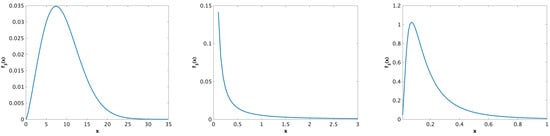
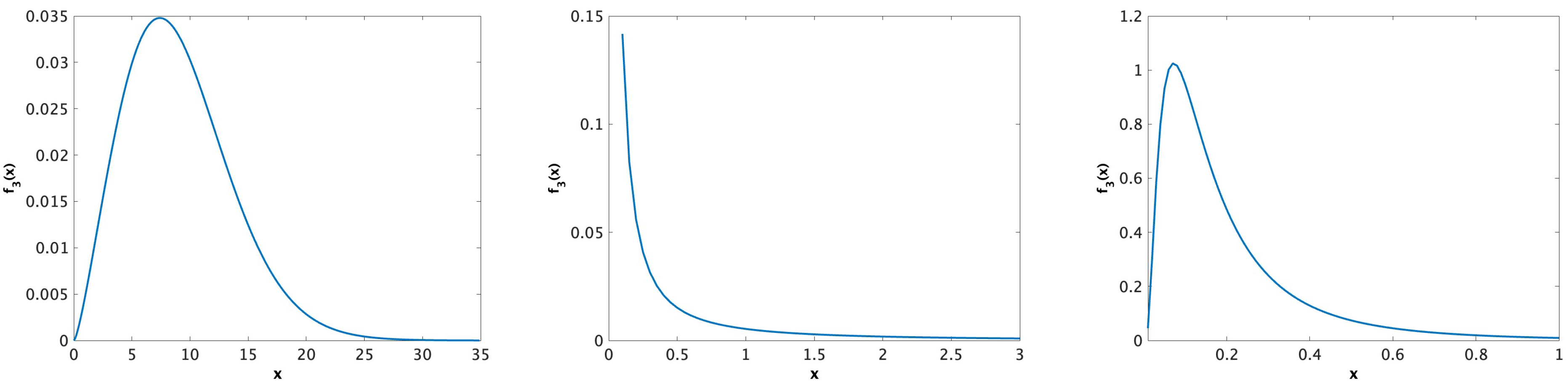
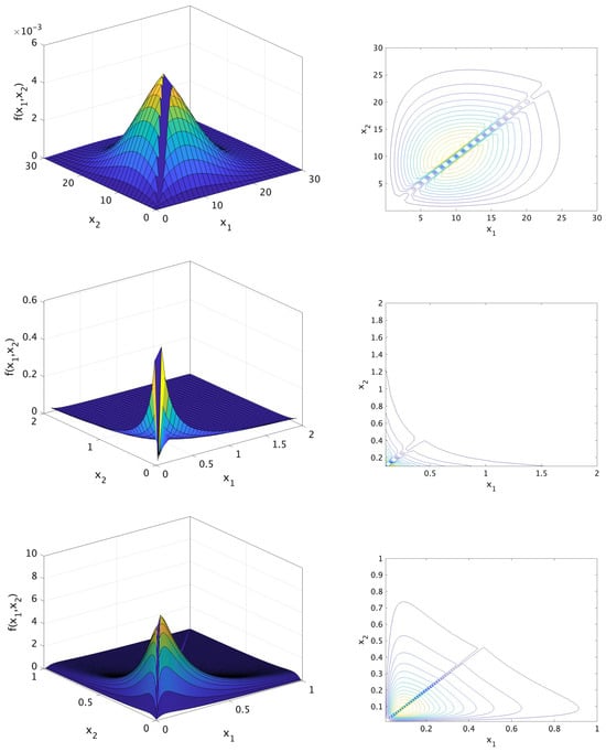
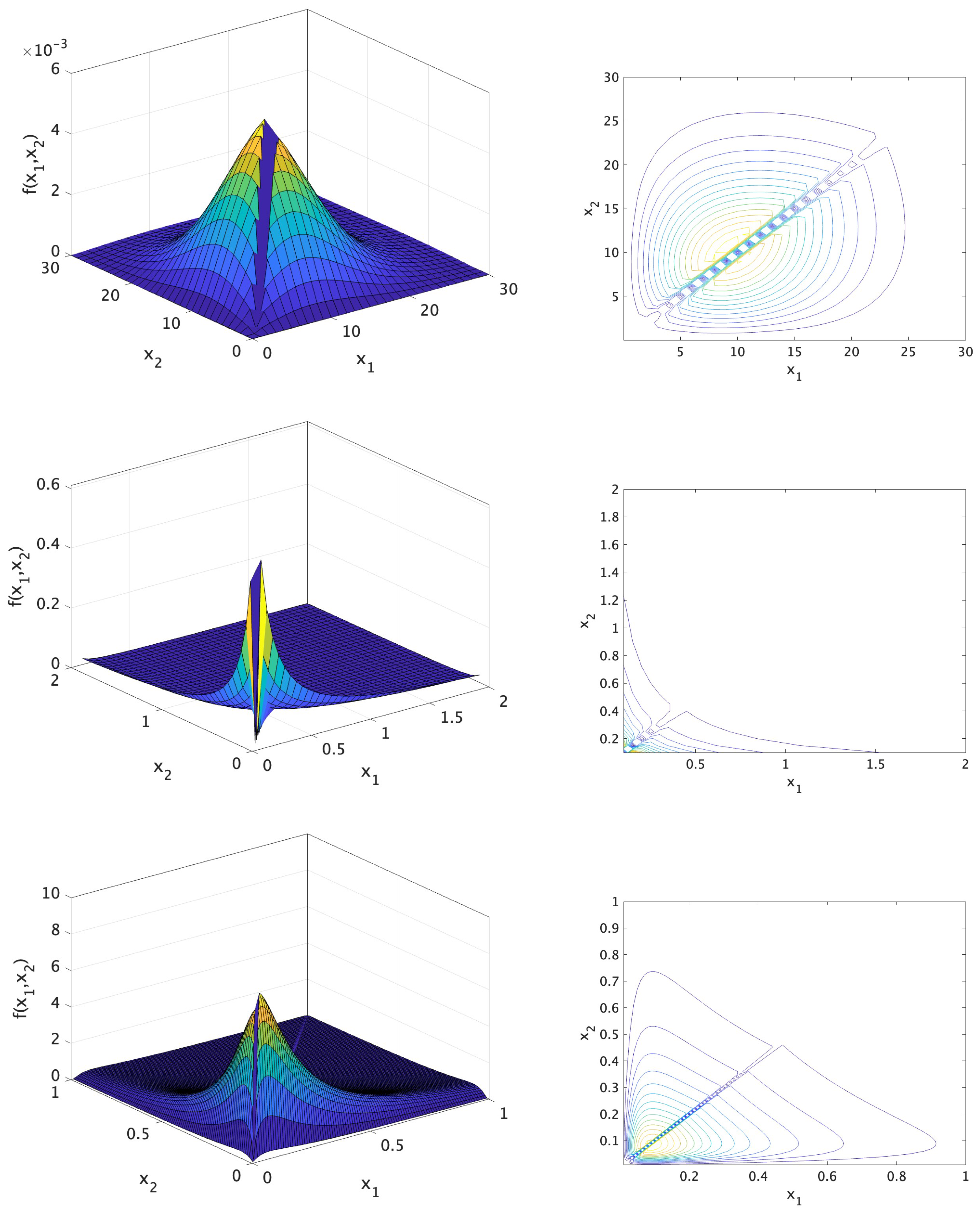
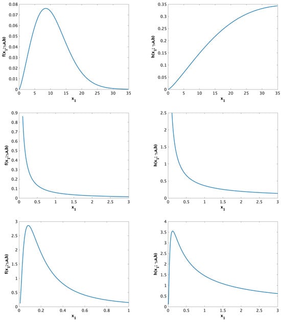
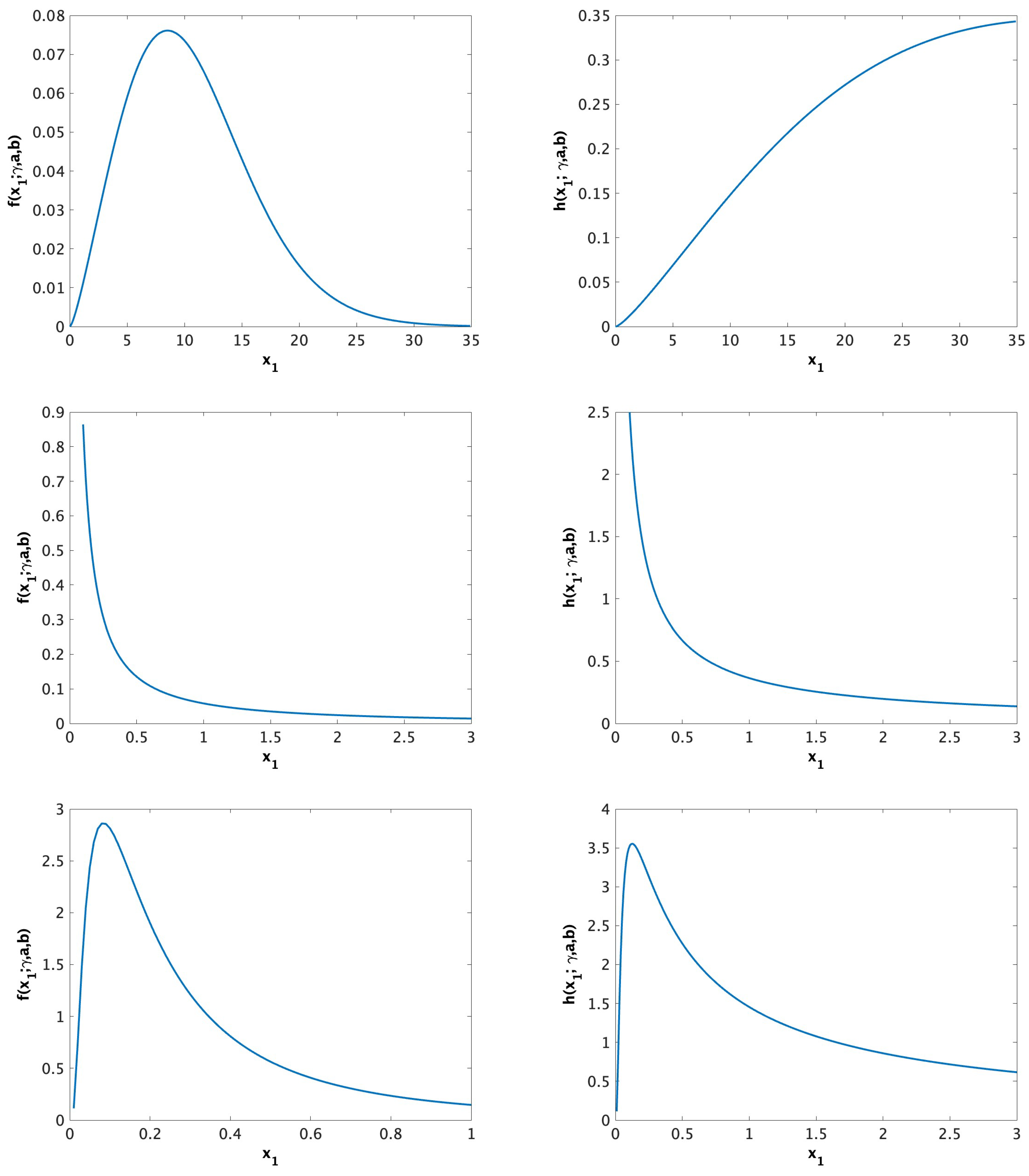
To illustrate the versatility of the new distribution, we generated graphs depicting both the continuous and singular components of the joint probability density function; see Figure 1 and Figure 2. Furthermore, we visualized the marginal probability density function and the marginal hazard rate function of $X_1$ across various sets of values of model parameters, as shown in Figure 3. Figure 3 shows that the marginal hazard rate function can exhibit increasing, decreasing, or unimodal behavior. This characteristic enhances the adaptability of this distribution, enabling it to effectively accommodate diverse sets of real-world data.

Figure 1. The singular part of the BBXII-IW$(\gamma ,a,b_1,b_2,b_3)$ when the following is the case: (1) Set 1: $\gamma =0.1, a=15, b_1=6, b_2=5, b_3=7$; (2) Set 2: $\gamma =0.1, a=1.5, b_1=3, b_2=4, b_3=2$; (3) Set 3: $\gamma =0.5, a=1, b_1=3$, $b_2=4$, $b_3=2$ (from left to right).

Figure 2. The continuous parts of the joint pdf and the corresponding contour plots of the BBXII-IW distribution at different values for the model parameters: (1) Set 1: $\gamma =0.1, a=15, b_1=6, b_2=5, b_3=7$; (2) Set 2: $\gamma =0.1, a=1.5, b_1=3, b_2=4, b_3=2$; (3) Set 3: $\gamma =0.5, a=1, b_1=3, b_2=4, b_3=2$ (from top to bottom).

Figure 3. The pdf and the hrf of the marginal distribution of $X_1$ when the following is the case: (1) Set 1: $\gamma =0.1, a=15, b_1=6, b_2=5, b_3=7$; (2) Set 2: $\gamma =0.1, a=1.5, b_1=3, b_2=4, b_3=2$; (3) Set 3: $\gamma =0.5, a=1$, $b_1=3$, $b_2=4, b_3=2$ (from top to bottom).

Marshall–Olkin Copula Representation

We now describe the dependence structure of the BBXII-IW distribution using the Marshall–Olkin (MO) copula. The BBXII-IW model is constructed by applying the MO copula to two univariate Burr XII Inverse Weibull (BXII-IW) distributions used as marginals. According to Sklar’s theorem, any bivariate survival function $S_{1,2}(x_1,x_2)$ with continuous marginal survival functions $S_{X_1}\left(x_1\right)$ and $S_{X_2}\left(x_2\right)$ can be expressed using a copula function C as follows:

$$S_{1,2}(x_1,x_2)=C(S_{X_1}\left(x_1\right),S_{X_2}\left(x_2\right)),\mathrm{for}\mathrm{all}(x_1,x_2)\in R^2,$$

as established in copula theory (see Nelsen [5]).

The Marshall–Olkin copula employed in this work is defined by

$$C_{{\theta }_1,{\theta }_2}(u_1,u_2)=u_1^{1-{\theta }_1}{u}_2^{1-{\theta }_2}min(u_1^{{\theta }_1},u_2^{{\theta }_2}),$$

where $0<{\theta }_1$ and ${\theta }_2<1$ are dependence parameters. Letting $u_j=S_{X_j}\left(x_j\right)$, where $X_j\sim \mathrm{BXII}-\mathrm{IW}(\gamma ,a,b_j+b_3)$, and defining ${\theta }_j={\displaystyle \frac{b_3}{b_j+b_3}}$ for $j=1,2$, the resulting joint survival function $S(x_1,x_2)$ corresponds to the expression derived in Equation (4).

5. Maximum Likelihood Estimation

The model parameters $\theta =(\gamma ,a,b_1,b_2,b_3)$ are estimated in this section using two different types of data: (1) bivariate data and (2) dependent competing risk data. Below are the details.

5.1. Bivariate Data

The bivariate data consist of n independent and identically distributed pairs of random variables $(X_{i1},X_{i2})$, $i=1,2,\cdots ,n$. In this study, we assume that $(X_{i1},X_{i2})$ follows the BBXII-IW$(\gamma ,a,b_1,b_2,b_3)$, for $i=1,2,\cdots ,n$. Therefore, the likelihood function of the given bivariate data is

$$L\left(\theta \right)=\prod _{i=1}^{n}f(x_{i1},x_{i2})$$

(11)

The likelihood function can be re-expressed as

$$\begin{array}{ccc}\hfill L\left(\theta \right)& =& \prod _{i=1}^n{\left[f_2(x_{1i},x_{2i})\right]}^{I[{\delta }_i=1]}{\left[f_1(x_{1i},x_{2i})\right]}^{I[{\delta }_i=2]}{\left[f_0\left(x_{1i}\right)\right]}^{I[{\delta }_i=0]}\hfill \end{array}$$

(12)

Here, the indicator variables ${\delta }_i,i=1,2,\dots ,n$, is defined as follows:

$${\delta }_i=\left\{\begin{array}{cc}0& \mathrm{if}{X}_{i1}=X_{i2},\\ 1& \mathrm{if}{X}_{i1}<X_{i2},\\ 2& \mathrm{if}{X}_{i1}>X_{i2}.\end{array}\right.$$

Substituting from Equation (5) into (12), we obtain the likelihood function as

$$\begin{array}{ccc}\hfill L\left(\theta \right)& =& {(b_2+b_3)}^{n_1}{a}^{n_1}{\gamma }^{n_1}{b}_1^{n_1}{(b_1+b_3)}^{n_2}{a}^{n_2}{\gamma }^{n_2}{b}_2^{n_1}{a}^{n_0}{\gamma }^{n_0}{b}_3^{n_0}\hfill \end{array}$$

(13)

$$\begin{array}{ccc}\hfill & & \prod _{i=1}^n{\left[1+{(e^{x_{1i}^{-\gamma }}-1)}^{-a}\right]}^{-(b_1+1)I[{\delta }_i=1]}{\left[1+{(-1+e^{x_{2i}^{-\gamma }})}^{-a}\right]}^{-(b_2+b_3+1)I[{\delta }_i=1]}\hfill \\ \hfill & & \prod _{i=1}^n{\left[{\left(x_{1i}{x}_{2i}\right)}^{(\gamma +1)}(e^{x_{1i}^{-\gamma }}-1)(e^{x_{2i}^{-\gamma }}-1)\right]}^{-I[{\delta }_i=1]}{\left[1+{(e^{x_{2i}^{-\gamma }}-1)}^{-a}\right]}^{-(b_2+1)I[{\delta }_i=2]}\hfill \\ \hfill & & \prod _{i=1}^n{\left[1+{(-1+e^{x_{1i}^{-\gamma }})}^{-a}\right]}^{-(b_1+b_3+1)I[{\delta }_i=2]}{\left[{\left(x_{1i}{x}_{2i}\right)}^{(\gamma +1)}(e^{x_{1i}^{-\gamma }}-1)(e^{x_{2i}^{-\gamma }}-1)\right]}^{-I[{\delta }_i=2]}\hfill \\ & & \prod _{i=1}^n{\left[1+{(e^{x_{1i}^{-\gamma }}-1)}^{-a}\right]}^{-(b_1+b_2+b_3+1)I[{\delta }_i=0]}{\left[{\left(x_{1i}\right)}^{(\gamma +1)}(e^{x_{1i}^{-\gamma }}-1)\right]}^{-I[{\delta }_i=0]}.\hfill \end{array}$$

(14)

The log-likelihood function is given by

$$\begin{array}{ccc}\hfill \mathcal{L}\left(\theta \right)& =& n_{1}ln(b_2+b_3)+n_{2}ln(b_1+b_3)+n_{1}ln{b}_1+n_{2}ln{b}_2+n_{0}ln{b}_3\hfill \\ \hfill & & +nln\left(a\gamma \right)-(b_1+1)\sum _{i=1}^{n}I[{\delta }_i=1]ln\left[1+{(e^{x_{1i}^{-\gamma }}-1)}^{-a}\right]\hfill \\ \hfill & & -(b_2+b_3+1)\sum _{i=1}^{n}I[{\delta }_i=1]ln\left[1+{(e^{x_{2i}^{-\gamma }}-1)}^{-a}\right]\hfill \\ \hfill & & -\sum _{i=1}^{n}I[{\delta }_i=1]\left[(\gamma +1)ln\left(x_{1i}{x}_{2i}\right)+ln(e^{x_{1i}^{-\gamma }}-1)+ln(e^{x_{2i}^{-\gamma }}-1)\right]\hfill \\ \hfill & & -(b_2+1)\sum _{i=1}^{n}I[{\delta }_i=2]ln\left[1+{(e^{x_{2i}^{-\gamma }}-1)}^{-a}\right]\hfill \\ \hfill & & -(b_1+b_3+1)\sum _{i=1}^{n}I[{\delta }_i=2]ln\left[1+{(e^{x_{1i}^{-\gamma }}-1)}^{-a}\right]\hfill \\ \hfill & & -\sum _{i=1}^{n}I[{\delta }_i=2]\left[(\gamma +1)ln\left(x_{1i}{x}_{2i}\right)+ln(e^{x_{1i}^{-\gamma }}-1)+ln(e^{x_{2i}^{-\gamma }}-1)\right]\hfill \\ \hfill & & -(b_1+b_2+b_3+1)\sum _{i=1}^{n}I[{\delta }_i=0]ln\left[1+{(e^{x_{1i}^{-\gamma }}-1)}^{-a}\right]\hfill \\ \hfill & & -\sum _{i=1}^{n}I[{\delta }_i=0]\left[(\gamma +1)ln\left(x_{1i}\right)+ln(e^{x_{1i}^{-\gamma }}-1)\right],\hfill \end{array}$$

(15)

where $n_j={\displaystyle \sum _{i=1}^n}I[{\delta }_i=j],j=0,1,2,$ with $I\left(A\right)=1$ if A is true and 0 otherwise.

To obtain the maximum likelihood estimates (MLEs) of the model parameters, we maximize the log-likelihood function with respect to these parameters. This involves the following steps:

• Set the First Partial Derivatives to Zero: Calculate the partial derivatives of the log-likelihood function with respect to each model parameter and set them equal to zero. These resulting equations are known as the likelihood equations.
• Solve the Likelihood Equations: Solve these equations simultaneously to find the MLEs of the model parameters.
• Verify the Solution Using the Fisher Information Matrix: At the solution, the Fisher Information Matrix (FIM), which comprises the second partial derivatives (the Hessian) of the log-likelihood function evaluated at the MLEs, should be positive definite. This ensures that the solution corresponds to a maximum of the log-likelihood function.

Below are the first partial derivatives of the log-likelihood function:

$$\begin{array}{ccc}\hfill {\displaystyle \frac{\partial \mathcal{L}}{\partial b_1}}& =& {\displaystyle \frac{n_1}{b_1}}+{\displaystyle \frac{n_2}{(b_1+b_3)}}-\sum _{j=0}^2\sum _{i=1}^{n}I[{\delta }_i=j]ln\left[1+{(e^{x_{1i}^{-\gamma }}-1)}^{-a}\right],\hfill \end{array}$$

(16)

$$\begin{array}{ccc}\hfill {\displaystyle \frac{\partial \mathcal{L}}{\partial b_2}}& =& {\displaystyle \frac{n_2}{b_2}}+{\displaystyle \frac{n_1}{(b_2+b_3)}}-\sum _{j=1}^2\sum _{i=1}^{n}I[{\delta }_i=j]ln\left[1+{(e^{x_{2i}^{-\gamma }}-1)}^{-a}\right]\hfill \\ \hfill & -& \sum _{i=1}^{n}I[{\delta }_i=0]ln\left[1+{(e^{x_{1i}^{-\gamma }}-1)}^{-a}\right],\hfill \end{array}$$

(17)

$$\begin{array}{ccc}\hfill {\displaystyle \frac{\partial \mathcal{L}}{\partial b_3}}& =& {\displaystyle \frac{n_2}{(b_1+b_3)}}+{\displaystyle \frac{n_1}{(b_2+b_3)}}+{\displaystyle \frac{n_0}{b_3}}-\sum _{i=1}^{n}I[{\delta }_i=2]ln\left[1+{(e^{x_{1i}^{-\gamma }}-1)}^{-a}\right]\hfill \\ \hfill & -& \sum _{i=1}^{n}I[{\delta }_i=1]ln\left[1+{(e^{x_{2i}^{-\gamma }}-1)}^{-a}\right]-\sum _{i=1}^{n}I[{\delta }_i=0]ln\left[1+{(e^{x_{1i}^{-\gamma }}-1)}^{-a}\right],\hfill \end{array}$$

(18)

$$\begin{array}{ccc}\hfill {\displaystyle \frac{\partial \mathcal{L}}{\partial a}}& =& {\displaystyle \frac{n}{a}}+(b_1+1)\sum _{i=1}^{n}I[{\delta }_i=1]{\displaystyle \frac{{(e^{x_{1i}^{-\gamma }}-1)}^{-a}ln(e^{x_{1i}^{-\gamma }}-1)}{1+{(e^{x_{1i}^{-\gamma }}-1)}^{-a}}}\hfill \\ \hfill & +& (b_2+b_3+1)\sum _{i=1}^{n}I[{\delta }_i=1]{\displaystyle \frac{{(e^{x_{2i}^{-\gamma }}-1)}^{-a}ln(e^{x_{2i}^{-\gamma }}-1)}{1+{(e^{x_{2i}^{-\gamma }}-1)}^{-a}}}\hfill \\ \hfill & +& (b_2+1)\sum _{i=1}^{n}I[{\delta }_i=2]{\displaystyle \frac{{(e^{x_{2i}^{-\gamma }}-1)}^{-a}ln(e^{x_{2i}^{-\gamma }}-1)}{1+{(e^{x_{2i}^{-\gamma }}-1)}^{-a}}}\hfill \\ \hfill & +& (b_1+b_3+1)\sum _{i=1}^{n}I[{\delta }_i=2]{\displaystyle \frac{{(e^{x_{1i}^{-\gamma }}-1)}^{-a}ln(e^{x_{1i}^{-\gamma }}-1)}{1+{(e^{x_{1i}^{-\gamma }}-1)}^{-a}}}\hfill \\ \hfill & +& (b_1+b_2+b_3+1)\sum _{i=1}^{n}I[{\delta }_i=0]{\displaystyle \frac{{(e^{x_{1i}^{-\gamma }}-1)}^{-a}ln(e^{x_{1i}^{-\gamma }}-1)}{1+{(e^{x_{1i}^{-\gamma }}-1)}^{-a}}},\hfill \end{array}$$

(19)

and

$$\begin{array}{ccc}\hfill {\displaystyle \frac{\partial \mathcal{L}}{\partial \gamma }}& =& {\displaystyle \frac{n}{\gamma }}-a(b_1+1)\sum _{i=1}^{n}I[{\delta }_i=1]{\displaystyle \frac{{(e^{x_{1i}^{-\gamma }}-1)}^{-a-1}{e}^{x_{1i}^{-\gamma }}ln\left(x_{1i}\right)}{1+{(e^{x_{1i}^{-\gamma }}-1)}^{-a}}}\hfill \\ \hfill & -& a(b_2+b_3+1)\sum _{i=1}^{n}I[{\delta }_i=1]{\displaystyle \frac{{(e^{x_{2i}^{-\gamma }}-1)}^{-a-1}{e}^{x_{2i}^{-\gamma }}ln\left(x_{2i}\right)}{1+{(e^{x_{2i}^{-\gamma }}-1)}^{-a}}}\hfill \\ \hfill & -& \sum _{i=1}^{n}I[{\delta }_i=1]\left(ln\left(x_{1i}{x}_{2i}\right)-{\displaystyle \frac{e^{x_{1i}^{-\gamma }}ln\left(x_{1i}\right)}{(e^{x_{1i}^{-\gamma }}-1)}}-{\displaystyle \frac{e^{x_{2i}^{-\gamma }}ln\left(x_{2i}\right)}{(e^{x_{2i}^{-\gamma }}-1)}}\right)\hfill \\ \hfill & -& a(b_2+1)\sum _{i=1}^{n}I[{\delta }_i=2]{\displaystyle \frac{{(e^{x_{2i}^{-\gamma }}-1)}^{-a-1}{e}^{x_{2i}^{-\gamma }}ln\left(x_{2i}\right)}{1+{(e^{x_{2i}^{-\gamma }}-1)}^{-a}}}\hfill \\ \hfill & -& a(b_1+b_3+1)\sum _{i=1}^{n}I[{\delta }_i=2]{\displaystyle \frac{{(e^{x_{2i}^{-\gamma }}-1)}^{-a-1}{e}^{x_{2i}^{-\gamma }}ln\left(x_{2i}\right)}{1+{(e^{x_{2i}^{-\gamma }}-1)}^{-a}}}\hfill \\ \hfill & -& \sum _{i=1}^{n}I[{\delta }_i=2]\left(ln\left(x_{1i}{x}_{2i}\right)-{\displaystyle \frac{e^{x_{1i}^{-\gamma }}ln\left(x_{1i}\right)}{(e^{x_{1i}^{-\gamma }}-1)}}-{\displaystyle \frac{e^{x_{2i}^{-\gamma }}ln\left(x_{2i}\right)}{(e^{x_{2i}^{-\gamma }}-1)}}\right)\hfill \\ \hfill & +& (b_1+b_2+b_3+1)\sum _{i=1}^{n}I[{\delta }_i=0]{\displaystyle \frac{{(e^{x_{1i}^{-\gamma }}-1)}^{-a-1}{e}^{x_{1i}^{-\gamma }}ln\left(x_{1i}\right)}{1+{(e^{x_{1i}^{-\gamma }}-1)}^{-a}}}\hfill \\ \hfill & -& \sum _{i=1}^{n}I[{\delta }_i=0]\left(ln\left(x_{1i}\right)-{\displaystyle \frac{e^{x_{1i}^{-\gamma }}ln\left(x_{1i}\right)}{(e^{x_{1i}^{-\gamma }}-1)}}\right).\hfill \end{array}$$

(20)

Note: The positive definiteness of the FIM indicates that the log-likelihood function has a local maximum at the estimated parameters.

Due to the complexity of the proposed distribution, the likelihood equations cannot be solved analytically. To address this, we employed numerical optimization techniques in R to estimate the five model parameters by maximizing the log-likelihood function directly rather than solving the traditional system of likelihood equations.

R provides several tools for solving systems of non-linear equations, including the nleqslv package, which implements Broyden’s and Newton’s methods with global strategies such as line search and trust region. The BB package offers Barzilai–Borwein spectral methods, particularly useful for high-dimensional problems, while the pracma package provides the fsolve function for root-finding in non-linear systems.

However, in this study, we used the optim function in R (version 4.4.2) (Appendix A.1) to perform numerical maximization of the log-likelihood. This approach circumvents the need to explicitly solve the non-linear likelihood equations and is well-suited for complex, parameter-rich models such as the one considered here. In the optim function, we used the “BFGS” method (Broyden–Fletcher–Goldfarb–Shanno) because it is efficient for smooth and differentiable likelihood functions. It provides fast convergence by utilizing gradient information to approximate the Hessian matrix, making it well-suited for maximum likelihood estimation problems.

The computational feasibility of the proposed estimation procedure has also been verified. Despite the complexity of the likelihood function, the number of parameters remains modest (five in total), and the use of efficient optimization routines such as the BFGS algorithm ensures that the estimation process scales well. Empirical evaluations in Section 7 confirm that the MLE procedure remains stable and computationally tractable for moderate to large sample sizes, making the method practical for real-world data applications.

5.2. Confidence Intervals

As discussed earlier, the maximum likelihood estimates (MLEs) of the model parameters cannot be derived analytically due to the complexity of the likelihood equations. Consequently, the exact sampling distribution of the MLEs is not available, and exact confidence intervals for the parameters cannot be obtained.

As an alternative, approximate confidence intervals can be constructed using the asymptotic normality of the MLEs. Specifically, under regularity conditions, the MLE $\widehat{\theta }$ is approximately normally distributed as $\widehat{\theta }\sim N(\theta ,\Sigma )$, where $\Sigma$ is the variance–covariance matrix of the estimators. For more details on this approximation, we refer to Cox and Hinkley [28] and Davison [29]. This matrix $\Sigma$ is typically derived from the inverse of the observed Fisher information matrix, which consists of the second-order partial derivatives of the log-likelihood function evaluated at the MLEs. These second derivatives can be obtained from Equations (16)–(20); however, they are omitted here for brevity. Based on this asymptotic result, an approximate $(1-\vartheta )100\%$ confidence interval for the parameter ${\theta }_j$ is given by

$${\widehat{\theta }}_j\pm z_{{\displaystyle \frac{\vartheta }{2}}}\mathrm{SE}\left({\widehat{\theta }}_j\right),j=1,2,3,4,5,$$

where $\mathrm{SE}\left({\widehat{\theta }}_j\right)=\sqrt{{\Sigma }_{jj}}$, and $z_{{\displaystyle \frac{\vartheta }{2}}}$ denotes the upper ${\displaystyle \frac{\vartheta }{2}}$ quantile of the standard normal distribution.

As we can see, it is tedious to obtain the variance–covariance matrix of the MLE estimators. Therefore, we can easily compute the bootstrap confidence intervals (Appendix A.2) of the model parameters without computing such a matrix. Below is the algorithm that can be applied to obtain the percentile confidence intervals (BPCIs):

• Given a simple random sample $(X_{1i},X_{2i})$ along with ${\delta }_i$, $i=1,2,\cdots ,n$, for the bivariate data discussed above, we carry out the steps outlined in points 2–4.
• Compute the MLE of the model parameters as described above. There is no need to compute the corresponding variance–covariance matrix.
• Simulate M samples with replacements from the given sample. For each simulated sample, compute the MLE of the model parameters.
• Use the M values of the MLEs obtained in step 3; we can compute the $(1-\vartheta )100\%$ BPCI as the ${\displaystyle \frac{\vartheta }{2}}{100}^{th}$ and $\left(1-{\displaystyle \frac{\vartheta }{2}}\right){100}^{th}$ percentiles.

6. Dependent Competing Risks Data

For dependent competing risk data, we observe a pair $(T,\delta )$, where T denotes the time to failure or death, and $\delta$ indicates the cause of failure. The procedure for generating such data is described as follows:

• A total of n identical and independent units (e.g., individuals or systems) are placed on a life test.
• Each unit is exposed to two competing fatal risks.
• For each unit i, where $i=1,2,\cdots ,n$, we observe the time to failure $T_i$ and the corresponding cause of failure ${\delta }_i$. The failure indicator ${\delta }_i$ is defined as follows:

  $${\delta }_i=\left\{\begin{array}{cc}1\hfill & \mathrm{if}\mathrm{risk}1\mathrm{causes}\mathrm{the}\mathrm{failure},\hfill \\ 2\hfill & \mathrm{if}\mathrm{risk}2\mathrm{causes}\mathrm{the}\mathrm{failure},\hfill \\ 3\hfill & \mathrm{if}\mathrm{the}\mathrm{cause}\mathrm{of}\mathrm{failure}\mathrm{is}\mathrm{unknown},\hfill \end{array}\right.$$

Given the dependent competing risk data $(T_i,{\delta }_i)$, $i=1,2,\cdots ,n$, the likelihood function is given as

$$L=\prod _{i=1}^n\prod _{j=1}^3{\left[f_j^{*}\left(t_i\right)\right]}^{I({\delta }_i=j)},$$

(21)

where

$$f_j^{*}\left(t\right)={\displaystyle \frac{b_{j}a\gamma e^{t^{-\gamma }}{t}^{-\gamma -1}{\left\{1+{\left(e^{t^{-\gamma }}-1\right)}^{-a}\right\}}^{-(b_1+b_2+b_3)}}{\left(e^{t^{-\gamma }}-1\right)\left[{\left(e^{t^{-\gamma }}-1\right)}^{-a}+1\right]}},j=1,2,3.$$

(22)

Substituting from (22) into (21), we obtain

$$L={\displaystyle \frac{b_1^{n_1}{b}_2^{n_2}{b}_3^{n_3}{\left(a\gamma \right)}^n{e}^{{\sum }_{i=1}^n{t}_i^{-\gamma }}{\prod }_{i=1}^n{t}_i^{-(\gamma +1)}{\prod }_{i=1}^n{\left\{1+{\left(e^{t_i^{-\gamma }}-1\right)}^{-a}\right\}}^{-(b_1+b_2+b_3)}}{{\prod }_{i=1}^n\left(e^{t_i^{-\gamma }}-1\right){\prod }_{i=1}^n\left[{\left(e^{t_i^{-\gamma }}-1\right)}^a+1\right]}}.$$

(23)

The logarithm of the likelihood function can be expressed as

$$\begin{array}{ccc}\hfill \mathcal{L}& =& \sum _{j=1}^3{n}_{j}log{b}_j+nlog\left(a\gamma \right)-(\gamma +1)\sum _{i=1}^{n}log(t_i)+\sum _{i=1}^n{t}_i^{-\gamma }-\sum _{i=1}^{n}log\left(e^{t_i^{-\gamma }}-1\right)+\hfill \\ & & -\sum _{i=1}^{n}log\left[{\left(e^{t_i^{-\gamma }}-1\right)}^a+1\right]-(b_1+b_2+b_3)\sum _{i=1}^{n}log\left\{1+{\left(e^{t_i^{-\gamma }}-1\right)}^{-a}\right\},\hfill \end{array}$$

(24)

where $n_j={\sum }_{i=1}^{n}I({\delta }_i=j)$, $j=1,2,3$.

To obtain the maximum likelihood estimators (MLEs) of the model parameters, we must maximize the likelihood function $\mathcal{L}$ concerning these parameters. This involves setting the first partial derivatives of $\mathcal{L}$ concerning the parameters to zero and subsequently solving the resulting system of five non-linear equations in the unknown parameters. It is worth noting that this system of non-linear equations lacks an analytical solution for the unknown parameters.

However, within this system of non-linear equations, there are three equations derived from the partial derivatives concerning $b_1$, $b_2$, and $b_3$, which can be solved to express $b_j$, where $j=1,2,3$, as functions of the other two parameters, $\gamma$ and a. These relationships are as follows:

$${\widehat{b}}_j=n_j/\sum _{i=1}^{n}log\left\{1+{\left(e^{t_i^{-\gamma }}-1\right)}^{-a}\right\}.$$

(25)

Substituting (25) into (23), we obtain ${\mathcal{L}}^{*}$ as a function in only two parameters $\gamma$ and a:

$$\begin{array}{ccc}\hfill {\mathcal{L}}^{*}(\gamma ,a)& =& \sum _{j=1}^3{n}_{j}log\left[n_j/\sum _{i=1}^{n}log\left\{1+{\left(e^{t_i^{-\gamma }}-1\right)}^{-a}\right\}\right]+nlog\left(a\gamma \right)+\hfill \\ & & -(\gamma +1)\sum _{i=1}^{n}log\left(t_i\right)+\sum _{i=1}^n{t}_i^{-\gamma }-\sum _{i=1}^{n}log\left(e^{t_i^{-\gamma }}-1\right)+\hfill \\ & & -\sum _{i=1}^{n}log\left[{\left(e^{t_i^{-\gamma }}-1\right)}^a+1\right]-n.\hfill \end{array}$$

(26)

To attain the maximum value of ${\mathcal{L}}^{*}$, it is necessary to address a non-linear system encompassing two equations, which can be derived by equating ${\displaystyle \frac{\partial {\mathcal{L}}^{*}}{\partial \gamma }}=0$ and ${\displaystyle \frac{\partial {\mathcal{L}}^{*}}{\partial a}}=0$. Importantly, the solutions to this system must adhere to the condition that the corresponding Fisher information matrix is positive definite. Here, we find the initial partial derivatives of ${\mathcal{L}}^{*}$:

$$\begin{array}{ccc}\hfill {\displaystyle \frac{\partial {\mathcal{L}}^{*}}{\partial \gamma }}& =& {\displaystyle \frac{n}{\gamma }}-{\displaystyle \frac{na\left({\displaystyle \sum _{i=1}^n}\frac{t_i^{-\gamma }log(t_i){\mathrm{e}}^{t_i^{-\gamma }}}{\left({\mathrm{e}}^{t_i^{-\gamma }}-1\right)\left(1+{\left({\mathrm{e}}^{t_i^{-\gamma }}-1\right)}^a\right)}\right)}{{\displaystyle \sum _{i=1}^n}log(1+{\left({\mathrm{e}}^{t_i^{-\gamma }}-1\right)}^{-a})}}-\sum _{i=1}^{n}log(t_i)+\sum _{i=1}^n\left[-t_i^{-\gamma }log\left(t_i\right)\right]+\hfill \\ & & \sum _{i=1}^n\left({\displaystyle \frac{t_i^{-\gamma }log(t_i){\mathrm{e}}^{t_i^{-\gamma }}}{{\mathrm{e}}^{t_i^{-\gamma }}-1}}\right)-a\sum _{i=1}^n\left({\displaystyle \frac{t_i^{-\gamma }log(t_i){\mathrm{e}}^{t_i^{-\gamma }}}{\left({\mathrm{e}}^{t_i^{-\gamma }}-1\right)\left({\left({\mathrm{e}}^{t_i^{-\gamma }}-1\right)}^a+1\right)}}\right),\hfill \end{array}$$

(27)

and

$$\begin{array}{ccc}\hfill {\displaystyle \frac{\partial {\mathcal{L}}^{*}}{\partial a}}& =& {\displaystyle \frac{n}{a}}+\sum _{i=1}^n{\displaystyle \frac{log\left(e^{t_i^{-\gamma }}-1\right)}{{\left(e^{t_i^{-\gamma }}-1\right)}^a+1}}+{\displaystyle \frac{n{\sum }_{i=1}^n{\displaystyle \frac{log\left(e^{t_i^{-\gamma }}-1\right)}{{\left(e^{t_i^{-\gamma }}-1\right)}^a+1}}}{{\sum }_{i=1}^{n}log\left\{1+{\left(e^{t_i^{\gamma }}-1\right)}^{-a}\right\}}}.\hfill \end{array}$$

(28)

Alternatively, we can use the optim function in R to obtain the MLEs of $\gamma$ and a. Once these estimates are obtained, we can use Equation (25) to derive the MLEs of the remaining model parameters.

7. Simulation Study

Random Sample Generation

Below is the algorithm that we can follow to generate bivariate samples from BBXII-IW distribution (Appendix A.3).

• Generate three independent random variate $U_i$ from BXII-IW$(\gamma ,a,b_i)$, $i=1,2,3$, using the following equation:

  $$U_i=exp\left\{-{\displaystyle \frac{1}{\gamma }}loglog\left(1+{\left[{\displaystyle \frac{1}{{(1-q_i)}^{1/b_i}}}-1\right]}^{-1/a}\right)\right\},\mathrm{where} q_i\sim U(0,1)$$
• Define $X_j=min\{U_j,U_3\},j=1,2$. This gives $(X_1,X_2)\sim \mathrm{BBXII-IW}(\gamma ,a,b_1,b_2,b_3)$.

To evaluate the model’s stability and its practical relevance across diverse theoretical frameworks, we execute a simulation experiment of the dual-variable framework employing two separate parameter specifications. The simulation adheres to the following protocol:

• Initialize Parameter Settings: Establish the observation count n and the model coefficients $\gamma ,a,b_1,b_2$, and $b_3$.
• Create Synthetic Datasets: Employing the stochastic generation approach detailed above, produce M artificial samples of $(X_1,X_2)$.
• Compute Statistical Estimates: For each sample from Step 2, calculate the following:
  • The maximum likelihood estimates (MLE) of the five parameters;
  • Their respective 95% confidence intervals.
• Assess Model Performance: Using the M replications from Step 3, calculate the following:

  (a)

  The average of the maximum likelihood point estimate (AMLE);

  (b)

  The estimation variance (the means squared error, MSE);

  (c)

  The interval precision measure by computing the average length of the confidence interval (ALCI);

  (d)

  The empirical containment rate and coverage probability (CP) of the CI.

The CTM and EV are computed as follows:

$$\begin{array}{cccc}\hfill \mathrm{AMLE}& ={\displaystyle \frac{{\sum }_{i=1}^M{\widehat{\theta }}^{\left(i\right)}}{M}},\hfill & \hfill \mathrm{MSE}& ={\displaystyle \frac{{\sum }_{i=1}^M{(\theta -{\widehat{\theta }}^{\left(i\right)})}^2}{M}},\hfill \\ \hfill \mathrm{AMLE}& ={\displaystyle \frac{{\sum }_{i=1}^M\left[{\widehat{\theta }}_U^{\left(i\right)}-{\widehat{\theta }}_L^{\left(i\right)}\right]}{M}},\hfill & \hfill CP& ={\displaystyle \frac{{\sum }_{i=1}^{M}I(\theta \in C{I}_i)}{M}},\hfill \end{array}$$

where ${\widehat{\theta }}^{\left(i\right)}$ represents the MLE of parameter $\theta$ ($\theta =\gamma ,a,b_1,b_2,b_3$). ${\theta }_L^{\left(i\right)}$ and ${\theta }_U^{\left(i\right)}$ are the lower and upper bounds of the confidence interval CI_i for the i-th sample ($i=1,2,\dots ,M$).

Table 1 presents the simulation outcomes for sample sizes $n=30,50,75,100$, and 150, with $M=10,000$, using two distinct parameter combinations. The analysis reveals these key findings:

Table 1. The estimation results for two sets of model parameters: Set I: $\gamma =0.1,a=15,b_1=6,$$b_2=5,$$b_3=7$; Set II: $\gamma =0.1,a=1.5,b_1=3,b_2=4,b_3=2$.

n	Par	AMLE	MSE	ALCI	CP	AMLE	MSE	ALCI	CP
		Set I				Set II
30	$\gamma$	0.103	0.00039	0.0737	95.43	0.1035	$4\times {10}^{-4}$	0.0741	95.4
	a	15.5532	9.11095	11.131	95.06	1.5469	0.08842	1.1071	94.85
	$b_1$	6.2194	1.38701	4.4511	95.38	3.1038	0.35865	2.2213	95.55
	$b_2$	5.1766	0.98169	3.7048	95.27	4.127	0.61926	2.9536	95.02
	$b_3$	7.2414	1.93274	5.1825	95.45	2.0707	0.15454	1.482	95.57
50	$\gamma$	0.1022	0.00022	0.0566	94.93	0.102	0.00022	0.0565	95.08
	a	15.2804	4.86538	8.4709	95.07	1.5325	0.05068	0.8496	95.16
	$b_1$	6.1343	0.80828	3.4006	95.02	3.0621	0.19993	1.6975	95.15
	$b_2$	5.1055	0.55533	2.8303	95.35	4.0831	0.35288	2.2635	94.77
	$b_3$	7.1353	1.08749	3.9555	95.06	2.0407	0.08981	1.1313	94.88
75	$\gamma$	0.1015	0.00015	0.0459	94.62	0.1016	0.00015	0.046	95.29
	a	15.2118	3.27406	6.8854	94.95	1.5212	0.03195	0.6885	95.25
	$b_1$	6.0924	0.51107	2.7576	95.33	3.0419	0.12714	1.3769	95.49
	$b_2$	5.0601	0.3593	2.2904	95.01	4.0498	0.22738	1.8331	95.28
	$b_3$	7.0954	0.70211	3.2116	95.27	2.0289	0.05715	0.9183	94.87
100	$\gamma$	0.1011	0.00011	0.0396	94.74	0.1011	0.00011	0.0396	94.83
	a	15.1504	2.41311	5.9388	94.81	1.5152	0.02338	0.5939	95.02
	$b_1$	6.0603	0.38025	2.3756	95.02	3.0311	0.09382	1.1882	94.99
	$b_2$	5.0506	0.26214	1.9798	94.8	4.0376	0.16765	1.5827	94.93
	$b_3$	7.0641	0.51518	2.7691	94.97	2.0214	0.04154	0.7924	95.28
150	$\gamma$	0.1006	$7\times {10}^{-5}$	0.0322	94.97	0.1008	$7\times {10}^{-5}$	0.0323	95.13
	a	15.119	1.52824	4.839	95.39	1.5087	0.01515	0.4829	95.19
	$b_1$	6.0331	0.24659	1.9309	94.87	3.0216	0.0619	0.9671	95.15
	$b_2$	5.0376	0.17395	1.6123	94.87	4.0248	0.10869	1.2882	95.19
	$b_3$	7.0399	0.3328	2.2532	95.35	2.013	0.02711	0.6443	95.01
200	$\gamma$	0.1006	$5\times {10}^{-5}$	0.0279	95.11	0.1004	$5\times {10}^{-5}$	0.0278	94.59
	a	15.0667	1.15753	4.1762	94.72	1.5085	0.01164	0.4181	95.12
	$b_1$	6.0259	0.18467	1.6703	95	3.0155	0.04565	0.8358	95.33
	$b_2$	5.0285	0.1304	1.3938	94.85	4.024	0.08184	1.1154	95.25
	$b_3$	7.0329	0.25045	1.9494	94.94	2.0072	0.0204	0.5564	95.07

• Parameter Estimate Convergence: The MLE techniques demonstrates progressive alignment with true parameter values as the sample size expands.
• Diminishing Estimation Variance: The EV for MLE shows consistent reduction with larger datasets, signaling enhanced estimation reliability.
• Increasing Interval Precision: The IPM exhibits steady improvement with sample size growth, indicating sharper statistical inference.
• Consistent Coverage Performance: The ECR maintains close proximity to the target 95% benchmark for MLE.

8. Applications

This section examines two distinct real-world datasets: one involving dependent competing risks data and the other comprising bivariate data. The primary objective is to demonstrate the practical applicability and effectiveness of the proposed model in realistic settings. By analyzing these datasets, we aim to illustrate how the proposed approach can be employed to address complex scenarios and provide meaningful insights in applied contexts.

8.1. Bivariate Data

The data used in this study is derived from the UEFA Champions League and is sourced from Meintanis [30]. The dataset consists of soccer matches, including cases where the home team scores at least one goal and instances when a goal is scored directly from a penalty kick, foul kick, or any other direct kick (referred to as kick goals) by any team under consideration. The variable $X_1$ in the dataset represents the time in minutes when the first kick goal is scored by any team, while $X_2$ represents the time in minutes when the first goal of any type is scored by the home team. The details of this data are shown in Table 2.

Table 2. UEFA Champion’s League data.

2005–2006	${\mathit{X}}_1$	${\mathit{X}}_2$	2004–2005	${\mathit{X}}_1$	${\mathit{X}}_2$
Lyon–Real Madrid	26	20	Internazionale–Bremen	34	34
Milan–Fenerbahce	63	18	Real Madrid–Roma	53	39
Chelsea–Anderlecht	19	19	Man. United–Fenerbahce	54	7
Club Brugge–Juventus	66	85	Bayern–Ajax	51	28
Fenerbahce–PSV	40	40	Moscow–PSG	76	64
Internazionale–Rangers	49	49	Barcelona–Shakhtar	64	15
Panathinaikos–Bremen	8	8	Leverkusen–Roma	26	48
Ajax–Arsenal	69	71	Arsenal–Panathinaikos	16	16
Man. United–Benfica	39	39	Dynamo Kyiv–Real Madrid	44	13
Real Madrid–Rosenborg	82	48	Man. United–Sparta	25	14
Villarreal–Benfica	72	72	Bayern–M. Tel Aviv	55	11
Juventus–Bayern	66	62	Bremen–Internazionale	49	49
Club Brugge–Rapid	25	9	Anderlecht–Valencia	24	24
Olympiacos–Lyon	41	3	Panathinaikos–PSV	44	30
Internazionale–Porto	16	75	Arsenal–Rosenborg	42	3
Schalke–PSV	18	18	Liverpool–Olympiacos	27	47
Barcelona–Bremen	22	14	M. Tel Aviv–Juventus	28	28
Milan–Schalke	42	42	Bremen–Panathinaikos	2	2
Rapid–Juventus	36	52

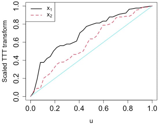
To gain a deeper understanding of why the BBXII-IW model presents a superior fit for this specific dataset, we employ a technique suggested by Aarset [31], known as the scaled TTT-Transform plot. This plot offers insights into the shape of the hazard function associated with a given distribution. For a lifetime distribution with a survival function denoted as $S\left(x\right)=1-F\left(x\right)$, the scaled TTT-transform is calculated as $\varphi \left(u\right)={\displaystyle \frac{H^{-1}\left(u\right)}{\mu }}$, where $H^{-1}\left(u\right)={\int }_0^{F^{-1}\left(u\right)}S\left(x\right)\mathrm{d}x$ is defined for $0<u<1$, and $\mu =H^{-1}\left(1\right)$.

In an empirical context, the scale TTT transform is approximated as ${\widehat{\varphi }}_n(i/n)={\displaystyle \frac{H_n^{-1}(i/n)}{H_n^{-1}\left(1\right)}}=\left[\left({\sum }_{j=1}^i{x}_{j:n}\right)+(n-i)x_{i:n}\right]/\left({\sum }_{j=1}^n{x}_{j:n}\right)$, where i ranges from 1 to n, and $x_{i:n},i=1,\dots ,n$ denotes the i-th order statistics of the sample. A seminal result by Aarset [31] establishes that the scaled TTT transform exhibits convexity (concavity) when the hazard rate decreases or increases. Additionally, for bathtub (unimodal) hazard rates, the scaled TTT-transform demonstrates a convex (concave) pattern followed by a concave (convex) one.

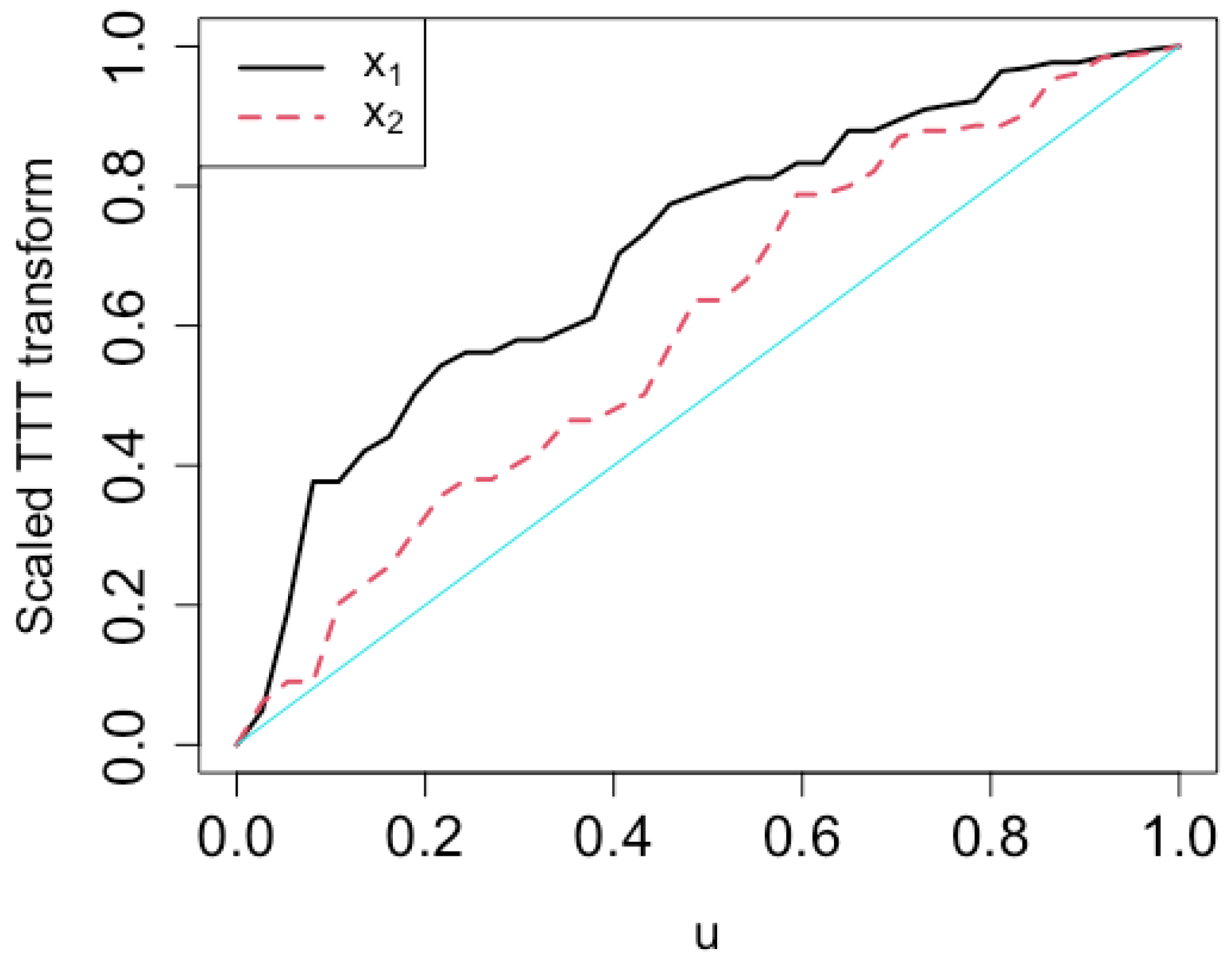
We visualize the scaled TTT transform individually for $X_1$ and $X_2$ in Figure 4. This plot serves as an initial exploratory tool, enabling us to delve into the distributional characteristics and behavior of the marginal data. Through this visualization, we infer that the hazard rate initially follows an ascending trajectory and subsequently transitions into a descending pattern as time advances or aging occurs. Given this discernible hazard rate trend, it is logical to expect that the BXII-IW distribution would emerge as a suitable candidate for modeling the marginal distribution of the data.

Figure 4. The scaled TTT transform plot for the marginal data $X_1$ and $X_2$ for UEFA data.

However, we investigate the applicability of the BXII and IW distributions, as well as their combined form BXII-IW, to determine whether the integration of IW and BXII distributions into the BXII-IW form results in an enhanced distribution. The MLEs of each model parameter, along with their associated log-likelihood values and Akaike Information Criterion (AIC) scores, are presented in Table 3. Additionally, we analyze fitting the marginal data using BXII-IR, BXII-IE, and LIW as sub-models of the BXII-IW distribution. The relevant results are outlined in Table 4, which includes the MLEs of the model parameters, the corresponding likelihood ($\mathcal{L}$), the likelihood ratio test statistic ($\Lambda$), degrees of freedom (df), and the p-value.

Table 3. Statistical analysis of the marginal data values $X_1$ and $X_2$ using the original models.

Model	MLE	$\mathcal{L}$	AIC	MLE	$\mathcal{L}$	AIC
	${\mathbf{X}}_{\mathbf{1}}$			${\mathbf{X}}_{\mathbf{2}}$
IW	$\widehat{\gamma }=0.3790999$	$-226.4274$	454.8548	$\widehat{\gamma }=0.4210359$	$-208.9056$	419.8113
BXII	$\widehat{a}=10.83184$	$-214.5671$	433.1343	$\widehat{a}=13.66833$	$-196.5861$	397.1723
	$\widehat{b}=0.02609962$			$\widehat{b}=0.02312574$
BXII-IW	$\widehat{\gamma }=0.05935803$	$-163.0454$	332.0907	$\widehat{\gamma }=0.0526701$	$-163.3399$	332.6798
	$\widehat{a}=24.76977$			$\widehat{a}=18.2096$
	$\widehat{b}=133.0863$			$\widehat{b}=101.6539$

Table 4. Statistical analysis of the marginal data values $X_1$ and $X_2$ using sub-models.

Model	${\mathit{H}}_0$	MLE	$-\mathcal{L}$	$\mathbf{\Lambda }$	df	p-Value
$X_1$
BXII-IR	$\gamma =2$	7.788442 0.01817231	214.397	102.703	1	0
BXII-IE	$\gamma =1$	21.45143 0.0132683	213.528	100.966	1	0
LIW	$a=1$	7.092002 0.03955422	214.5646	103.038	1	0
Full Mode l	–	0.05935803 24.76977 133.0863	163.045	–	–	–
$X_2$
BXII-IR	$\gamma =2$	8.355803 0.01894421	196.255	65.830	1	$4.44\times {10}^{-16}$
BXII-IE	$\gamma =1$	17.01133 0.01880013	194.835	65.830	1	$4.44\times {10}^{-16}$
LIW	$a=1$	6.251462 0.05051344	196.5939	66.508	1	$3.33\times {10}^{-16}$
Full Model	–	0.0526701 18.2096 101.6539	163.340	–	–	–

Upon reviewing the outcomes presented in Table 3 and Table 4, it becomes apparent that the BXII-IW distribution provides a more favorable fit for both marginal datasets when contrasted with the IW and BXII distributions, as evidenced by its lower AIC value. Moreover, all three examined sub-models (BXII-IR, BXII-IE, and LIW) should be dismissed for fitting the marginal data ($X_1$ and $X_2$) when compared to the BXII-IW distribution at any level of significance.

These findings suggest that the BXII-IW distribution may provide a better fit for the current bivariate dataset. To explore this further, the BBXII-IW distribution is employed and its performance is compared against three existing models: the BEGIE model (Sarhan et al. [22]), the BVGE model (Kundu and Gupta [32]), and the BGLFR model (Sarhan et al. [16]). Table 5 reports the maximum likelihood estimates (MLEs) of the parameters for each model, along with the corresponding log-likelihood values ($\mathcal{L}$) and AIC values. In addition, Table 6 summarizes the estimation results for various sub-models of the BBXII-IW distribution.

Table 5. Statistical analysis of the bivariate data $(X_1,X_2)$.

Model	MLE	$\mathcal{L}$	AIC
BEGIE	$\widehat{\lambda }=70.31$, $\widehat{\gamma }=2.1$, ${\widehat{\alpha }}_1=0.223$, ${\widehat{\alpha }}_2=0.066$, ${\widehat{\alpha }}_3=0.169$	$-315.141$	640.282
BVGE	${\widehat{\alpha }}_1=1.351$, ${\widehat{\alpha }}_2=0.465$, ${\widehat{\alpha }}_3=1.153$, $\widehat{\beta }=0.039$	$-296.94$	601.88
BGLFR	${\widehat{\alpha }}_1=0.492$, ${\widehat{\alpha }}_2=0.166$, ${\widehat{\alpha }}_3=0.411$, $\widehat{\beta }=2.013\times {10}^{-4}$,	$-293.38$	596.76
	$\widehat{\gamma }=8.051\times {10}^{-4}$
BBXII-IW	$\widehat{\gamma }=0.05$, $\widehat{a}=22.8$, ${\widehat{b}}_1=95.6$, ${\widehat{b}}_2=224.0$, ${\widehat{b}}_3=213.5$	$-289.64$	589.28

Table 6. Statistical analysis of the marginal data values $(X_1,X_2)$ using sub-models.

Model	MLE	$\mathcal{L}$	AIC	$\mathbf{\Lambda }$	df	p-Value
BBXII-IR	$\widehat{a}=5.195$, ${\widehat{b}}_1=0.0078$,	$-355.39$	718.78	131.5	1	0
	${\widehat{b}}_2=0.0161$, ${\widehat{b}}_3=0.0215$
BBXII-IE	$\widehat{a}=8.405$, ${\widehat{b}}_1=0.0095$,	$-353.68$	715.36	128.09	1	0
	${\widehat{b}}_2=0.020$, ${\widehat{b}}_3=0.026$
BLIW	$\widehat{\gamma }=6.569$, ${\widehat{b}}_1=0.0123$	$-355.73$	719.46	132.19	1	0
	${\widehat{b}}_2=0.0254$, ${\widehat{b}}_3=0.034$
BBXII-IW	$\widehat{\gamma }=0.05$, $\widehat{a}=22.8$, ${\widehat{b}}_1=95.6$	$-289.64$	589.28	–	–	–
	${\widehat{b}}_2=224.0$, ${\widehat{b}}_3=213.5$

The results presented in Table 5 indicate that the BBXII-IW distribution offers the best fit to the data among the considered models—BEGIE, BVGE, and BGLFR—as evidenced by its lowest AIC value. Furthermore, Table 6 demonstrates that all sub-models of the BBXII-IW distribution, namely BBXII-IR, BBXII-IE, and BLIW, are significantly outperformed by the full BBXII-IW model and thus are statistically rejected in favor of it.

8.2. Diabetic Retinopathy Application

Diabetic retinopathy is a progressive ocular condition that affects the retinal blood vessels and can lead to vision impairment or even complete blindness in individuals with diabetes. To address the risk of blindness—a major concern for diabetic patients—the National Eye Institute in Bethesda, Maryland, conducted a controlled experimental study involving 71 patients. In this study, one eye of each patient was randomly selected to receive laser therapy. Researchers recorded the time to blindness onset and indicated whether the treated eye, the untreated eye, or both became blind.

The primary goal of this experiment was to evaluate whether laser treatment can effectively delay the onset of blindness in diabetic retinopathy patients. The resulting dataset, summarized in Table 7, includes two possible failure events—blindness in either or both eyes—making it well-suited for analysis under a dependent competing risk framework.

Table 7. Diabetic retinopathy data.

i	1	2	3	4	5	6	7	8	9	10	11	12
$t_i$	266	91	154	285	583	547	79	622	707	469	93	1313
${\delta }_i$	1	2	2	0	1	2	1	0	2	2	1	2
i	13	14	15	16	17	18	19	20	21	22	23	24
$t_i$	805	344	790	125	777	306	415	307	637	577	178	517
${\delta }_i$	1	1	2	2	2	1	1	2	2	2	1	2
i	25	26	27	28	29	30	31	32	33	34	35	36
$t_i$	272	1137	1484	315	287	1252	717	642	141	407	356	1653
${\delta }_i$	0	0	1	1	2	1	2	1	2	1	1	0
i	37	38	39	40	41	42	43	44	45	46	47	48
$t_i$	427	699	36	667	588	471	126	350	350	663	567	966
${\delta }_i$	2	1	2	1	2	0	1	2	1	0	2	0
i	49	50	51	52	53	54	55	56	57	58	59	60
$t_i$	203	84	392	1140	901	1247	448	904	276	520	485	248
${\delta }_i$	0	1	1	2	1	0	2	2	1	1	2	2
i	61	62	63	64	65	66	67	68	69	70	71
$t_i$	503	423	285	315	727	210	409	584	355	1302	227
${\delta }_i$	1	2	2	2	2	2	2	1	1	1	2

Sarhan et al. [17] previously analyzed this dataset using the bivariate Chen distribution (BCD), characterized by four parameters: ${\alpha }_1$, ${\alpha }_2$, ${\alpha }_3$, and $\beta$. They obtained maximum likelihood estimates of ${\widehat{\alpha }}_1=0.0012$, ${\widehat{\alpha }}_2=0.0015$, ${\widehat{\alpha }}_3=0.0004$, and $\widehat{\beta }=0.2722$, with a corresponding log-likelihood value of ${\widehat{\mathcal{L}}}_{\mathrm{BCD}}=-581.26$ and AIC = 1170.52. Their findings indicated that the BCD provided a good fit for the data.

In this study, we extend the investigation by applying the BBXII-IW distribution along with its sub-models—BBXII-IR, BBXII-IE, and BLIW—to the same dataset. Through a comparative analysis of model performance, we aim to identify the distribution that best captures the underlying structure of the data. The findings are expected to provide further insight into the effectiveness of laser therapy in delaying vision loss among patients with diabetic retinopathy.

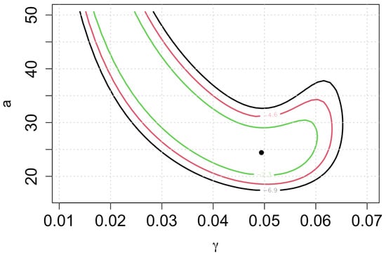
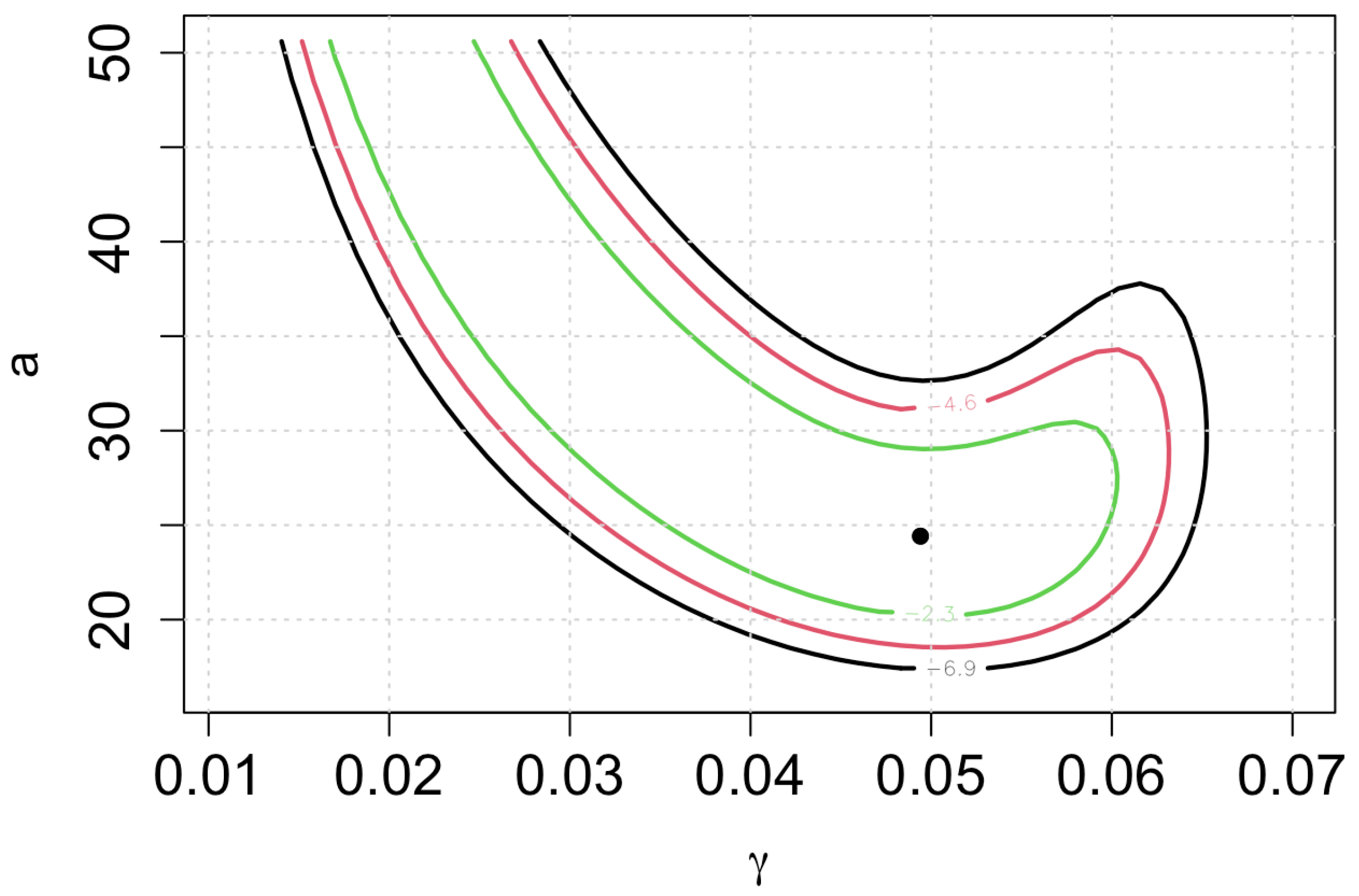
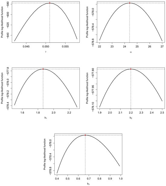
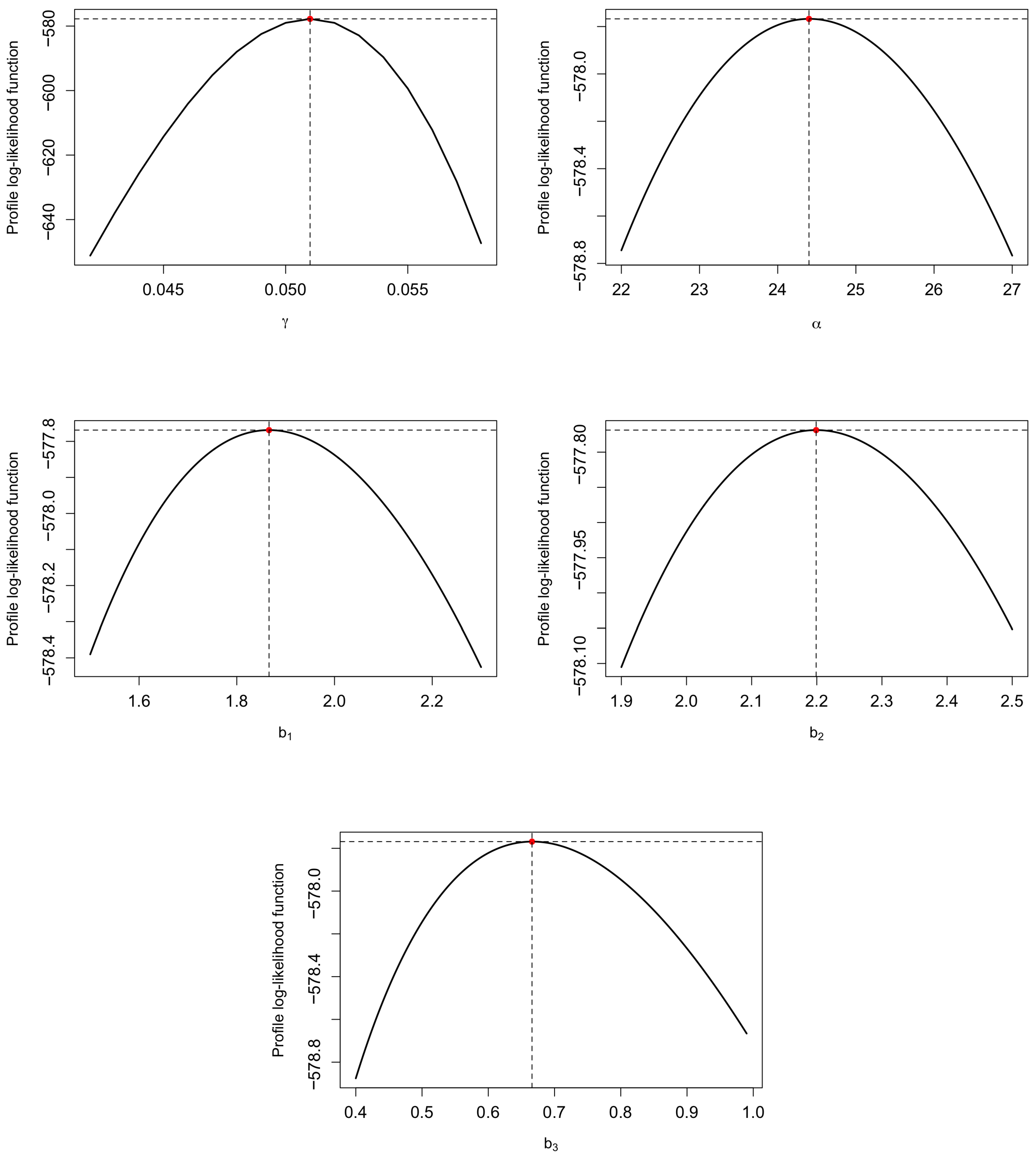
Figure 5 displays the contour plot of the reduced log-likelihood function for $(\gamma ,a)$, as defined in Equation (26). In addition, to illustrate the uniqueness of the maximum likelihood estimates (MLEs), the profile log-likelihood functions for each of the five parameters in the full BBXII-IW model are plotted, as shown in Figure 6.

Figure 5. The contour plot of ${\mathcal{L}}^{*}(\gamma ,a)$ using diabetic retinopathy data.

Figure 6. The profile log-likelihood function of the full model parameters using diabetic retinopathy data.

Table 8 presents the results for the full BBXII-IW model along with its sub-models, BBXII-IR, BBXII-IE, and BLIW, including the MLEs of model parameters, log-likelihood values, AIC scores, likelihood ratio test statistics, degrees of freedom, and corresponding p-values. The findings clearly indicate that all sub-models are significantly outperformed by the full BBXII-IW distribution and should therefore be rejected in its favor for modeling the diabetic retinopathy dataset. Additionally, based on AIC comparisons, the BBXII-IW model demonstrates a superior fit to the current dataset compared to the bivariate Chen distribution (BCD) used by Sarhan et al. [17].

Table 8. Statistical analysis of the diabetic retinopathy data.

Model	MLE	$\mathcal{L}$	AIC	$\mathbf{\Lambda }$	df	p-Value
BBXII-IR	$\widehat{a}=0.899$, ${\widehat{b}}_1=0.036$,	$-697.47$	1402.94	237.17	1	0
	${\widehat{b}}_2=0.043$, ${\widehat{b}}_3=0.013$
BBXII-IE	$\widehat{a}=1.669$, ${\widehat{b}}_1=0.039$,	$-697.34$	1402.67	219.39	1	0
	${\widehat{b}}_2=0.046$, ${\widehat{b}}_3=0.014$
BLIW	$\widehat{\gamma }=0.352$, ${\widehat{b}}_1=0.194$	$-704.08$	1416.16	232.87	1	0
	${\widehat{b}}_2=0.216$, ${\widehat{b}}_3=0.059$
BBXII-IW	$\widehat{\gamma }=0.051$, $\widehat{a}=24.32$, ${\widehat{b}}_1=1.87$	$-577.77$	1165.54	–	–	–
	${\widehat{b}}_2=2.120$, ${\widehat{b}}_3=0.669$

The standard errors (SEs) of the maximum likelihood estimates (MLEs) for the five model parameters are given as follows:

$$\begin{array}{c}\hfill \begin{array}{c}SE\left(\widehat{\gamma }\right)=0.0119,SE\left(\widehat{a}\right)=2.1314,SE\left({\widehat{b}}_1\right)=4.0987,\\ SE\left({\widehat{b}}_2\right)=4.8176,SE\left({\widehat{b}}_3\right)=1.4848.\end{array}\end{array}$$

The asymptotic confidence intervals (ACIs) and the percentile bootstrap confidence intervals (Bootstrap-P CIs) for these parameters are summarized in Table 9.

Table 9. The $95\%$ ACIs and Bootstrap-P CIs) for the parameters $b_1$, $b_2$, $b_3$, $\alpha$, and $\gamma$.

Parameters	MLE	Bootstraps-P CIs
$b_1$	{0.04708, 0.05492}	{0.0496, 0.0589}
$b_2$	{13.18916, 35.45084}	{15.2561, 39.2414}
$b_3$	{1.37304, 2.35696}	{0.8150, 1.7324}
a	{0.96904, 3.42296}	{1.2818, 3.7567}
$\gamma$	{0.44164, 0.89636}	{0.4366, 0.8381}

Finally, to assess the effectiveness of the laser surgery, we conduct the following hypothesis test:

$$\begin{array}{cc}\hfill H_0& :b_1=b_2(\mathrm{laser}\mathrm{surgery}\mathrm{is}\mathrm{ineffective})\hfill \\ \hfill H_1& :b_1\ne b_2(\mathrm{laser}\mathrm{surgery}\mathrm{is}\mathrm{effective})\hfill \end{array}$$

To analyze this test, we employ the likelihood ratio test (LRT) statistic, which follows a chi-square distribution with one degree of freedom. Using the provided data, the estimated parameters under the null hypothesis are as follows:

$$\widehat{\gamma }=0.053,\widehat{a}=25.212,{\widehat{b}}_1={\widehat{b}}_2=1.452,{\widehat{b}}_3=0.489,$$

with a log-likelihood value of $-578.1$. The computed LRT statistic is $0.668$, and the corresponding p-value is $0.414$.

Given this outcome, we do not have sufficient evidence to reject $H_0$, indicating that laser surgery was not significantly effective.

9. Conclusions and Future Work

In this study, we introduced a novel bivariate distribution within the Marshall–Olkin framework by leveraging the competing risks model. The proposed Bivariate Burr XII Inverse Weibull (BBXII-IW) distribution is constructed using three independent univariate random variables following the Burr XII Inverse Weibull (BXII-IW) distribution. Thanks to its ability to capture diverse hazard rate behaviors—including decreasing, upside-down, and increasing forms—the BBXII-IW distribution serves as a flexible generalization of several well-known models, such as the BXII-Inverse Rayleigh (BXII-IR), BXII-Inverse Exponential (BXII-IE), Log-Logistic IW (LogL-IW), and Lomax IW (LIW) distributions.

We derived key statistical properties of the BBXII-IW distribution and demonstrated its applicability in modeling dependent competing risks and bivariate data. Using maximum likelihood estimation, we efficiently estimated the unknown parameters and validated the method’s performance on real-world datasets. Comparative analyses with existing models, including the IW and BXII distributions, were conducted using hypothesis tests, confirming the superior flexibility and fit of the BBXII-IW distribution.

Future Research Directions

To further enhance the applicability and theoretical foundations of the BBXII-IW model, the following research avenues could be explored:

• Scalable Approximations: Recently, distributed data mining frameworks have gained attention for handling massive datasets spread across multiple computing agents. One such method is the Log-Scale Quantization in Distributed First-Order Methods (Doostmohammadian et al. [33]), which achieves scalability by distributing computation and communication efficiently. In contrast, our approach employs a centralized estimation procedure, which benefits from full-data access and yields high-precision estimates but may face limitations in memory or speed with extremely large datasets. A potential extension of our work involves adapting the BBXII-IW estimation framework to distributed environments by developing scalable approximations of the log-likelihood function or leveraging distributed optimization algorithms. This could enable broader applicability of the model to big data scenarios in distributed computing settings.
• Bayesian Inference: Develop Bayesian estimation methods, possibly incorporating Markov Chain Monte Carlo (MCMC) techniques, to improve parameter estimation robustness.
• Censored Data Modeling: Extend the model to accommodate right-censored, left-censored, and interval-censored data, common in survival analysis.
• Regression Extensions: Incorporate covariate effects into the BBXII-IW framework to enable broader applications in medical and engineering studies.
• Multivariate Generalizations: Expand the model to higher dimensions for handling more complex dependence structures in multivariate lifetime data.
• Copula-Based Approaches: Investigate connections between the BBXII-IW model and copula-based methods for dependent competing risks.

The BBXII-IW distribution provides a versatile and powerful tool for modeling complex dependencies in reliability and survival analysis. Future work in these directions could further solidify its theoretical and practical relevance.

Appendix A.1. MLE Estimation Using optim()

• Input: Bivariate data {(X1i, X2i), $\delta$i} for i = 1 to n

• Initialize: $\theta$_init = (gamma0, a0, b1_0, b2_0, b3_0)

• Define: Log-likelihood function l(theta) based on Equation (15)

• Call:

•  optim(par = theta_init,

•     fn = -l(theta),

•     method = "BFGS",

•     control = list(maxit = 1000))

• Output: MLE estimates theta.hat= (gamma.hat, a.hat,b1.hat, b2.hat, b3.hat)

Appendix A.2. Bootstrap Confidence Intervals (BPCIs)

• Input: Original sample {(X1i, X2i), deltai}, number of resamples M,

• confidence level (1 - alpha)

• Step 1: Estimate original parameters theta.hat using MLE

• Step 2: For m = 1 to M:

•   - Sample with replacement n observations from original data

•   - Compute theta^(m) using MLE on resampled data

• Step 3: For each parameter theta_j:

•   - Compute empirical percentiles:

•       CI_j = [theta.hat_j^(alpha/2), theta.hat_j^(1-alpha/2)]

• Output: (1 - alpha)100% Bootstrap CI for each theta_j

Appendix A.3. Data Simulation from BBXII-IW Distribution

• Input: Parameters gamma, a, b1, b2, b3; sample size n

• For i = 1 to n:

•     1. Generate q1, q2, q3 ~ Uniform(0,1)

•     2. For j = 1 to 3:

•       Uj = exp{--(1/gamma)*log[log(1+(1/(1--qj)^(1/bj)-1)^(-1/a))]}

•     3. Set:

•       X1 = min(U1, U3)

•       X2 = min(U2, U3)

•     4. Store (X1, X2)

• Output: Simulated dataset {X1i, X2i} for i = 1 to n

References

- Crowder, M.J. Classical Competing Risks; Chapman & Hall/CRC: Boca Raton, FL, USA, 2001. [Google Scholar]
- Ren, J.; Gui, W. Statistical analysis of adaptive type-II progressively censored competing risks for Weibull models. Appl. Math. Model. 2021, 98, 323–342. [Google Scholar] [CrossRef] [Scilit]
- Wang, L.; Tripathi, Y.M.; Lodhi, C. Inference for Weibull competing risks model with partially observed failure causes under generalized progressive hybrid censoring. J. Comput. Appl. Math. 2020, 368, 112537. [Google Scholar] [CrossRef] [Scilit]
- Mahto, A.K.; Lodhi, C.; Tripathi, Y.M.; Wang, L. Inference for partially observed competing risks model for Kumaraswamy distribution under generalized progressive hybrid censoring. J. Appl. Stat. 2021, 49, 2064–2092. [Google Scholar] [CrossRef] [Scilit]
- Nelsen, R.B. An Introduction to Copulas, 2nd ed.; Springer: New York, NY, USA, 2006. [Google Scholar]
- Duchateau, L.; Janssen, P. The Frailty Model; Springer: Berlin/Heidelberg, Germany, 2008. [Google Scholar]
- Wang, Y.C.; Emura, T.; Fan, T.H.; Lo, S.M.S.; Wilke, R.A. Likelihood-based inference for a frailty-copula model based on competing risks failure time data. Qual. Reliab. Eng. Int. 2020, 36, 1622–1638. [Google Scholar] [CrossRef] [Scilit]
- Gorfine, M.; Hsu, L. Frailty-based competing risks model for multivariate survival data. Biometrics 2011, 67, 415–426. [Google Scholar] [CrossRef] [Scilit]
- Lo, S.M.S.; Wilke, R.A. A copula model for dependent competing risks. J. R. Stat. Soc. C-Appl. 2010, 59, 359–376. [Google Scholar] [CrossRef] [Scilit]
- Fan, T.H.; Wang, Y.F.; Ju, S.K. A competing risks model with multiply censored reliability data under multivariate Weibull distributions. IEEE. Trans. Reliab. 2019, 68, 462–475. [Google Scholar] [CrossRef] [Scilit]
- Xu, A.; Fang, G.; Zhuang, L.; Gu, C. A multivariate student-t process model for dependent tail-weighted degradation data. IISE Trans. 2024, 57, 1071–1087. [Google Scholar] [CrossRef] [Scilit]
- Xu, A.; Wang, R.; Weng, X.; Wu, Q.; Zhuang, L. Strategic integration of adaptive sampling and ensemble techniques in federated learning for aircraft engine remaining useful life prediction. Appl. Soft Comput. 2025, 175, 113067. [Google Scholar] [CrossRef] [Scilit]
- Marshall, A.W.; Olkin, I. A multivariate exponential distribution. J. Am. Stat. Assoc. 1967, 62, 30–44. [Google Scholar] [CrossRef]
- Kotz, S.; Balakrishnan, N.; Johnson, N.L. Continuous Multivariate Distributions; John Wiley and Sons: New York, NY, USA, 2000. [Google Scholar]
- Sarhan, A.M.; Balakrishnan, N. A new class of bivariate distributions and its mixture. J. Multivar. Anal. 2007, 98, 1508–1527. [Google Scholar] [CrossRef] [Scilit]
- Sarhan, A.M.; Hamilton, D.C.; Smith, B.; Kundu, D. The bivariate generalized linear failure rate distribution and its multivariate extension. Comput. Stat. Data Anal. 2011, 55, 644–654. [Google Scholar] [CrossRef] [Scilit]
- Sarhan, A.M.; Apaloo, J.; Kundu, D. A new bivariate lifetime distribution: Properties, estimations and its extension. Commun. Stat.-Simul. Comput. 2024, 53, 879–896. [Google Scholar] [CrossRef] [Scilit]
- Bai, X.; Shi, Y.; Liu, B.; Fu, Q. Statistical inference of Marshall Olkin bivariate Weibull distribution with three shocks based on progressive interval-censored data. Commun. Stat. Simul. Comput. 2019, 48, 637–654. [Google Scholar] [CrossRef] [Scilit]
- Bakouch, A.S.; Moala, F.A.; Saboor, A.; Samad, H. A bivariate Kumaraswamy-exponential distribution with application. Math. Slovaca 2019, 69, 1185–1212. [Google Scholar] [CrossRef] [Scilit]
- Kilany, N.M.; El-Qareb, F.G. Modelling bivariate failure time data via bivariate extended Chen distribution. Stoch. Environ. Res. Risk Assess. 2023, 37, 3517–3525. [Google Scholar] [CrossRef] [Scilit]
- Manshi, T.; Sarhan, A.M.; Smith, B. A new bivariate distribution with applications on dependent competing risks data. Int. J. Stat. Probab. 2023, 12, 1927–7040. [Google Scholar] [CrossRef] [Scilit]
- Sarhan, A.M.; Gomaa, R.S.; Magar, A.M.; Alsadat, N. Bivariate exponentiated generalized inverted exponential distribution with applications on dependent competing risks data. AIMS Math. 2024, 9, 29439–29473. [Google Scholar] [CrossRef] [Scilit]
- Shrahili, M. A generalization of the Inverse Weibull model: Properties and applications. Ain Shams Eng. J. 2021, 12, 2057–2071. [Google Scholar] [CrossRef] [Scilit]
- Yousof, H.M.; Afify, A.Z.; Hamedani, G.G.; Aryal, G. The Burr X generator of distributions for lifetime data. J. Stat. Theory Appl. 2017, 16, 288–305. [Google Scholar] [CrossRef] [Scilit]
- Bhatti, F.A.; Hamedani, G.; Yousof, H.M.; Ali, A.; Ahmad, M. On Modified Burr XII-Inverse Exponential Distribution: Properties, Characterizations, and Applications. J. Biostat. Biom. 2018. Available online: https://epublications.marquette.edu/math_fac/62 (accessed on 22 December 2025).
- Kumar, C.S.; Nair, S.R. On Log-Inverse Weibull Distribution and Its Properties. Am. J. Math. Manag. Sci. 2018, 37, 144–167. [Google Scholar] [CrossRef] [Scilit]
- Goual, H.; Yousof, H.M.; Masoom, A.M. Lomax inverse Weibull model: Properties, applications, and a modified Chi-squared goodness-of-fit test for validation. J. Nonlinear Sci. Appl. 2020, 13, 330–353. [Google Scholar] [CrossRef] [Scilit]
- Cox, D.R.; Hinkley, D.V. Theoretical Statistics; Chapman and Hall: London, UK, 1974. [Google Scholar]
- Davison, A.C. Statistical Models, 1st ed.; Cambridge Series in Statistical and Probabilistic 408 Mathematics; Cambridge University Press: Cambridge, UK, 2008. [Google Scholar]
- Meintanis, S.G. Test of fit for marshall-olkin distributions with applications. J. Stat. Plan. Inference 2007, 137, 3954–3963. [Google Scholar] [CrossRef] [Scilit]
- Aarset, M.V. How to Identify Bathtub Hazard Rate. IEEE Trans. Reliab. 1987, R-36, 106–108. [Google Scholar] [CrossRef] [Scilit]
- Kundu, D.; Gupta, R.D. Bivariate generalized exponential distribution. J. Multivar. Anal. 2009, 100, 581–593. [Google Scholar] [CrossRef] [Scilit]
- Doostmohammadian, M.; Qureshi, M.I.; Khalesi, M.H.; Rabiee, H.R.; Khan, U.A. Log-Scale Quantization in Distributed First-Order Methods: Gradient-Based Learning From Distributed Data. IEEE Trans. Autom. Sci. Eng. 2025, 22, 10948–10959. [Google Scholar] [CrossRef] [Scilit]
Disclaimer/Publisher’s Note: The statements, opinions and data contained in all publications are solely those of the individual author(s) and contributor(s) and not of MDPI and/or the editor(s). MDPI and/or the editor(s) disclaim responsibility for any injury to people or property resulting from any ideas, methods, instructions or products referred to in the content. |
© 2025 by the authors. Licensee MDPI, Basel, Switzerland. This article is an open access article distributed under the terms and conditions of the Creative Commons Attribution (CC BY) license.