Dynamics Behavior of a Predator-Prey Diffusion Model Incorporating Hunting Cooperation and Predator-Taxis

Abstract

In this paper, we consider a predator-prey diffusion model incorporating hunting cooperation and predator-taxis. Firstly, we establish the global existence of a classical solution for the model in any spatial dimension. Secondly, we analyze the stability/instability caused by predator-taxis, and we observe that predator-taxis play a key role in inducing stability changes. Specifically, if the positive equilibrium is stable for the corresponding reaction-diffusion model, the attractive predator-taxis can further stabilize the system, while the repulsive predator-taxis may lead to a change in spatial stability, if the positive equilibrium is unstable for the corresponding reaction-diffusion model, the attractive predator-taxis makes the model remain unstable, while the repulsive predator-taxis has a stabilizing effect. Finally, numerical simulations are employed to validate the obtained results.

1. Introduction

The predator-prey relationship is a common phenomenon in nature and has garnered significant attention in the field of biomathematics research. Through conducting a investigation into the predator-prey model, we can reveal the evolution law of populations.

Hunting cooperation is a prevalent form of species interaction, which refers to the cooperative behavior exhibited by certain predators in the process of capturing prey. Hunting cooperation plays an important role in maintaining ecological diversity and regulating population density. Hunting cooperation can occur between individuals of the same species, such as lions, wild chimpanzees, fish, ants, birds, and so on [1,2,3,4,5]. Additionally, hunting cooperation behavior may also exist between different species, such as cheetahs and jackals preying on deer or badgers and coyotes targeting ground squirrels [6].

To reveal the impact of hunting cooperation by predators on species extinction, Duarte et al. [7] investigated a tri-trophic food chain model incorporative cooperative hunting, and they found that predators were more sensitive to extinction when hunting cooperation increased. Berec [8] considered hunting cooperation in the predator-prey model where the Holling II functional response is employed. Berec found that hunting cooperation exerts a destabilizing influence on predator-prey dynamics. Alves and Hilker [9] proposed that the attack rate of a predator species would increase with the increase in predator density due to foraging promotion. Therefore, they established a series of predator-prey models with hunting cooperation and Holling type functional responses, and concluded that cooperative hunting can improve the persistence of predator populations. Fu and Zhang [10] studied a Holling II type predator-prey diffusion model incorporative hunting cooperation

$$\left\{\begin{array}{cc}{u}_t=d_1\Delta u+\mathit{\sigma }u\left(1-{\displaystyle \frac{u}{\mathit{\kappa }}}\right)-{\displaystyle \frac{(1+\mathit{\alpha }v)uv}{1+h(1+\mathit{\alpha }v)u}},\hfill & x\in \Omega ,t>0,\hfill \\ v_t=d_2\Delta v+{\displaystyle \frac{(1+\mathit{\alpha }v)uv}{1+h(1+\mathit{\alpha }v)u}}-v,\hfill & x\in \Omega ,t>0,\hfill \end{array}\right.$$

(1)

where u, v denote prey and predator population densities, respectively. $\mathit{\sigma }$ and $\mathit{\kappa }$ are the per capita birth rate and carrying capacity for prey species, h designates the average hunting time of a predator for prey, $\mathit{\alpha }$ represents the rate of predator cooperation in hunting. Fu and Zhang [10] investigated linear stability and Turing instability of positive constant steady states, and analyzed the existence and stability for the Hopf bifurcated periodic solutions of this model.

In predator-prey models, the phenomenon of predators moving towards areas with higher prey density, known as prey-taxis, has been extensively studied. In 1987, Kareiva and Odell [11] first proposed an ecological model with prey-taxis to elucidate the directional movement of species. In the following decades, scholars have established numerous models with prey-taxis to investigate the dynamic relationship between predators and prey [12,13,14]. Recently, a novel form of predator-taxis has been developed and distinguished from prey-taxis, in which prey escapes from areas with a high predator density to avoid being captured. This means that the prey is moving in the direction of the predator. Several researchers have also explored and constructed several ecological models involving predator-taxis, see [15,16,17]. These models assumed that prey would move toward a lower density of predators to avoid dangerous situations.

Hunting cooperation and predator-taxis are prevalent in real ecosystems, so to better describe biological phenomena, we discuss the following predator-prey diffusion model that incorporates hunting cooperation and predator-taxis

$$\left\{\begin{array}{cc}{u}_t=d_1\Delta u+\nabla ·(\mathit{\chi }u\nabla v)+\mathit{\sigma }u\left(1-{\displaystyle \frac{u}{\mathit{\kappa }}}\right)-{\displaystyle \frac{(1+\mathit{\alpha }v)uv}{1+h(1+\mathit{\alpha }v)u}},\hfill & x\in \Omega ,t>0,\hfill \\ v_t=d_2\Delta v+{\displaystyle \frac{(1+\mathit{\alpha }v)uv}{1+h(1+\mathit{\alpha }v)u}}-v,\hfill & x\in \Omega ,t>0,\hfill \\ {\mathsf{\partial }}_{\mathit{\nu }}u={\mathsf{\partial }}_{\mathit{\nu }}v=0,\hfill & x\in \mathsf{\partial }\Omega ,t>0,\hfill \\ u(x,0)=u_0\left(x\right),v(x,0)=v_0\left(x\right),\hfill & x\in \Omega ,\hfill \end{array}\right.$$

(2)

where $\Omega$ is a bounded domain in ${\mathbb{R}}^n(n\ge 1)$, $\mathit{\nu }$ represents the outward unit normal vector to $\mathsf{\partial }\Omega$, the homogeneous zero-flux condition ensures that (2) is self-contained for $x\in \mathsf{\partial }\Omega$. Additionally, the initial data $u_0\left(x\right)$, $v_0\left(x\right)$ are smooth non-negative functions that are not identically zero. The term $-\nabla ·(\mathit{\chi }u\nabla v)$ denotes the directional movement of prey, and $\mathit{\chi }$ represent the sensitivity coefficient of predator-taxis. In particular, when $\mathit{\chi }<0$, the prey will move in the direction of the gradient of predators because of group defense when sensing the risk of predation, and then the predator–taxi is attracted; when $\mathit{\chi }>0$, it means that the prey exhibits an opposite movement direction for the gradient of predator, aiming to evade predation, and the predator-taxi is called repulsive. The model (2) well describes the effects of predator-taxis and hunting cooperation on a predator-prey diffusion model. From the perspective of mathematical research, by studying the dynamic behavior of the model (2), we can understand the relationship between species in the ecosystem more clearly so as to provide some theoretical support for maintaining a balance of the ecosystem and preventing species extinction.

The organization of this paper is as follows. Section 2 presents the global existence of a classical solution to model (2). In Section 3, we analyze the instability caused by predator-taxis for positive equilibrium in the model (2). Section 4 uses numerical simulations to verify the theoretical results. Finally, concise conclusions are provided in Section 5.

2. Global Existence of Classical Solution

In this section, we prove the global existence of a solution for the model (2) in any spatial dimensions. Moreover, throughout this section, we denote $C_i(i=1,2,3,\cdots )$ by generic positive constants that may differ from line to line. For simplicity, write ${\int }_{\Omega }wdx$ instead of ${\int }_{\Omega }w$.

2.1. Local Existence and Preliminary

We firstly employ the abstract theorem of the quasilinear parabolic system [18,19] to establish the local existence of a solution for model (2).

Lemma 1. 

Assume the initial data $(u_0\left(x\right),v_0\left(x\right))\in {\left[W^{1,p}(\Omega )\right]}^2$ with $p>n$ and $u_0\left(x\right),v_0\left(x\right)\ge 0(\not\equiv 0)$. Then, we have the following:

(i) 

There exists a positive constant $T_{max}$ such that model (2) admits a unique local-in-time classical solution $\left(u\right(x,t),v(x,t\left)\right)$, which satisfies;

$$(u(x,t),v(x,t))\in {\left(C(\overline{\Omega }\times [0,T_{max}))\cap C^{2,1}(\overline{\Omega }\times (0,T_{max}))\right)}^2.$$

(ii) 

There exists a constant $M_1>0$ such that;

$${\parallel u(·,t)\parallel }_{L^1(\Omega )}+{\parallel v(·,t)\parallel }_{L^1(\Omega )}\le M_{1}forallt\in (0,T_{max}).$$

(3)

(iii) 

There exists a constant $M_2>0$ such that;

$$0<v(x,t)\le M_2,u(x,t)>0forall(x,t)\in \overline{\Omega }\times (0,T_{max}).$$

(4)

(iv) 

If $T_{max}<\infty$, we have.

$$\underset{t\nearrow T_{max}}{lim\; sup}\left({\parallel u(·,t)\parallel }_{L^{\infty }(\Omega )}+{\parallel v(·,t)\parallel }_{W^{1,\infty }(\Omega )}\right)=\infty .$$

(5)

Proof. 

The local existence and uniqueness of the solution to (2) follows from Theorem 7.3 and Corollary 9.3 in [18] or Theorem 14.4 and 14.6 in [19], and the extensibility criterion (5) can be obtained directly from Theorem 15.5 in [19]. By utilizing the strong maximum principle on model (2), it can be find that $u(x,t)>0$ and $v(x,t)>0$ in $\overline{\Omega }\times (0,T_{max})$.

To prove (ii), we integrate the first two equations of (2) over $\Omega$, which implies that

$$\begin{array}{cc}{\displaystyle {\displaystyle \frac{d}{dt}}{\int }_{\Omega }(u+v)}\hfill & {\displaystyle =\mathit{\sigma }{\int }_{\Omega }u\left(1-{\displaystyle \frac{u}{\mathit{\kappa }}}\right)-{\int }_{\Omega }v={\int }_{\Omega }\left((\mathit{\sigma }+1)u-{\displaystyle \frac{\mathit{\sigma }}{\mathit{\kappa }}}{u}^2\right)-{\int }_{\Omega }(u+v)}\hfill \\ \hfill & {\displaystyle \le {\int }_{\Omega }{\displaystyle \frac{\mathit{\kappa }{(\mathit{\sigma }+1)}^2}{4\mathit{\sigma }}}-{\int }_{\Omega }(u+v)\le {\displaystyle \frac{\mathit{\kappa }{(\mathit{\sigma }+1)}^2|\Omega |}{4\mathit{\sigma }}}-{\int }_{\Omega }(u+v).}\hfill \end{array}$$

(6)

By employing the Gronwall inequality, one obtains (3).

Next, we establish the upper bound of $v(x,t)$, by the second equation in (2) and $u,v>0$, we have

$$\left\{\begin{array}{cc}{v}_t-d_2\Delta v={\displaystyle \frac{(1+\mathit{\alpha }v)uv}{1+h(1+\mathit{\alpha }v)u}}-v<{\displaystyle \frac{1}{h}}v,\hfill & x\in \Omega ,t>0,\hfill \\ {\mathsf{\partial }}_{\mathit{\nu }}v=0,\hfill & x\in \mathsf{\partial }\Omega ,t>0,\hfill \\ v(x,0)=v_0\left(x\right),\hfill & x\in \Omega .\hfill \end{array}\right.$$

(7)

Hence, we easily obtain that there exists a constant $M_2>0$ such that $v(x,t)\le M_2$ from Theorem 3.1 in [20] and the comparison principle. □

To establish the global-in-time of the solution, we next recall some preliminary estimates. For $p\in (1,\infty )$, we represent the sectorial operator by A and define it as

$$Az:=-\Delta z\mathrm{for}z\in D\left(A\right):=\left\{z\in W^{2,p}(\Omega ):{\displaystyle \frac{\mathsf{\partial }z}{\mathsf{\partial }\mathit{\nu }}}=0,z\in \mathsf{\partial }\Omega \right\},$$

(8)

similarly, we denote $A_{d_1}u:=-d_1\Delta u,A_{d_2}v:=-d_2\Delta v,$ where $A_{d_1}$ and $A_{d_2}$ possess the same properties as A with a scaling. Here, we will give some properties for A, but applying the properties of $A_{d_1}$ and $A_{d_2}$ in the subsequent discussion.

Lemma 2 

([21]). Let $k\in \{0,1\}$, $p\in [1,\infty ]$, and $q\in (1,\infty )$. Then, for any $z\in D\left({(A+1)}^{\mathit{\vartheta }}\right)$, there exists $C_1>0$ such that

$${\parallel z\parallel }_{W^{k,p}(\Omega )}\le C_1{\parallel {(A+1)}^{\mathit{\vartheta }}z\parallel }_{L^q(\Omega )},$$

(9)

where $\mathit{\vartheta }\in (0,1)$ and satisfies

$$k-{\displaystyle \frac{n}{p}}<2\mathit{\vartheta }-{\displaystyle \frac{n}{q}}.$$

If, in addition $q\ge p$, then for any $u\in L^p(\Omega )$, there exist $C_2>0$ and $\mathit{\beta }>0$ such that

$${\parallel (A+1)}^{\mathit{\vartheta }}{e}^{-t(A+1)}{z\parallel }_{L^q(\Omega )}\le C_2{t}^{-\mathit{\vartheta }-\frac{n}{2}(\frac{1}{p}-\frac{1}{q})}{e}^{-\mathit{\beta }t}{\parallel z\parallel }_{L^p(\Omega )},$$

(10)

with the associated heat semigroup ${\left\{e^{-t(A+1)}\right\}}_{t\ge 0}$ is known to map $L^p(\Omega )$ into $D({(A+1)}^{\mathit{\vartheta }})$. Additionally, for all $p\in (1,\infty )$ and $\mathit{\eta }>0$, there exist $C_3>0$ and $\mathit{\zeta }>0$ such that

$${\parallel (A+1)}^{\mathit{\vartheta }}{e}^{-tA}{\nabla ·z\parallel }_{L^p(\Omega )}\le C_3{t}^{-\mathit{\vartheta }-\frac{1}{2}-\mathit{\eta }}{e}^{-\mathit{\zeta }t}{\parallel z\parallel }_{L^p(\Omega )}$$

(11)

is valid for any ${\mathbb{R}}^n$–valued $z\in L^p(\Omega )$.

Lemma 3 

(Gagliardo-Nirenberg interpolation inequality [22]). Suppose $p,q\in [1,\infty ]$, and $\mathit{\varsigma }\in (0,p)$, where $p<\infty$ for $q=n$, and $p\le \frac{qn}{n-q}$ for $q<n$. Then, for $\mathit{\vartheta }\in (0,1]$ given by: $-\frac{n}{p}=(1-\frac{n}{q})\mathit{\vartheta }-\frac{n}{\mathit{\varsigma }}(1-\mathit{\vartheta })$ and some $C_4>0$, we have

$${\parallel z\parallel }_{L^p(\Omega )}\le C_4{(\parallel \nabla z\parallel }_{L^q(\Omega )}^{\mathit{\vartheta }}{\parallel z\parallel }_{L^{\mathit{\varsigma }}(\Omega )}^{1-\mathit{\vartheta }}+{\parallel z\parallel }_{L^{\mathit{\varsigma }}(\Omega )})$$

(12)

for any $z\in W^{1,q}(\Omega )\cap L^{\mathit{\varsigma }}(\Omega )$.

2.2. Global Existence of Solution

In this section, we study the solution to model (2) and its global existence. To begin with, we provide a bound for ${\parallel v(·,t)\parallel }_{W^{1,\infty }(\Omega )}$.

Lemma 4. 

Assume $\left(u\right(x,t),v(x,t\left)\right)$ to be a classical solution of (2). Then there exists a constant $M_3>0$ such that

$${\parallel v(·,t)\parallel }_{W^{1,\infty }(\Omega )}\le M_{3}forallt\in (0,T_{max}).$$

Proof. 

Let $\mathit{\tau }\in (0,T_{max})$ be chosen, satisfying $\mathit{\tau }<1$, fix $q>n$ and $\mathit{\vartheta }\in (\frac{1}{2}(1+\frac{n}{q}),1)$. Rewrite the equation of v in (2) as follows

$${\displaystyle \frac{\mathsf{\partial }v}{\mathsf{\partial }t}}-d_2\Delta v+v={\displaystyle \frac{(1+\mathit{\alpha }v)uv}{1+h(1+\mathit{\alpha }v)u}},$$

(13)

in view of the variation-of-constants formula, one yields

$${\displaystyle v(·,t)=e^{-t(A_{d_2}+1)}{v}_0+{\int }_0^t{e}^{-(t-s)(A_{d_2}+1)}{\displaystyle \frac{(1+\mathit{\alpha }v)uv}{1+h(1+\mathit{\alpha }v)u}}ds.}$$

From (9) and (10), we find that for any $t\in (\mathit{\tau },T_{max})$,

$$\begin{array}{cc}\hfill & {\parallel v(·,t)\parallel }_{W^{1,\infty }(\Omega )}\hfill \\ \le \hfill & C_1{\parallel {(A_{d_2}+1)}^{\mathit{\vartheta }}v\parallel }_{L^q(\Omega )}\hfill \\ \le \hfill & {\displaystyle C_1{C}_2{t}^{-\mathit{\vartheta }}{e}^{-\mathit{\beta }t}{\parallel v_0\parallel }_{L^q(\Omega )}+C_1{C}_2{\int }_0^t{(t-s)}^{-\mathit{\vartheta }}{e}^{-\mathit{\beta }(t-s)}{∥\frac{(1+\mathit{\alpha }v)uv}{1+h(1+\mathit{\alpha }v)u}∥}_{L^q(\Omega )}ds}\hfill \\ \le \hfill & {\displaystyle C_1{C}_2{t}^{-\mathit{\vartheta }}{e}^{-\mathit{\beta }t}\parallel v_0{\parallel }_{L^q(\Omega )}+{\displaystyle \frac{1}{h}}{C}_1{C}_2{\int }_0^t{(t-s)}^{-\mathit{\vartheta }}{e}^{-\mathit{\beta }(t-s)}{\parallel v\parallel }_{L^q(\Omega )}ds}\hfill \\ \le \hfill & {\displaystyle C_3{t}^{-\mathit{\vartheta }}+C_3{\int }_0^t{(t-s)}^{-\mathit{\vartheta }}{e}^{-\mathit{\beta }(t-s)}ds}\hfill \\ \le \hfill & {\displaystyle C_3{t}^{-\mathit{\vartheta }}+C_3{\int }_0^{\infty }{\mathit{\zeta }}^{-\mathit{\vartheta }}{e}^{-\mathit{\beta }\mathit{\zeta }}d\mathit{\zeta }}\hfill \\ \le \hfill & C_3{\mathit{\tau }}^{-\mathit{\vartheta }}+C_3\Gamma (1-\mathit{\vartheta }),\hfill \end{array}$$

where $\Gamma (·)$ is a Gamma function, then $\Gamma (1-\mathit{\vartheta })>0$ due to $0<\mathit{\vartheta }<1$. Therefore, we can obtain

$${\parallel v(·,t)\parallel }_{W^{1,\infty }(\Omega )}\le M_3.$$

□

Next, we state $u(x,t)$ is uniformly bounded in $L^p(\Omega )$ for any $p\ge 2$

Lemma 5. 

Assume $\left(u\right(x,t),v(x,t\left)\right)$ to be a classical solution of (2). Then for any $p\in [2,\infty )$, there exists a constant $M_4>0$ such that

$${\parallel u(·,t)\parallel }_{L^p(\Omega )}\le M_{4}forallt\in (0,T_{max}).$$

Proof. 

For $p\ge 2$, the equation of u in (2) is multiplied by $u^{p-1}$ and then integrated over $\Omega$, one has

$$\begin{array}{cc}\hfill & {\displaystyle {\displaystyle \frac{1}{p}}{\displaystyle \frac{d}{dt}}{\int }_{\Omega }{u}^p}\hfill \\ =\hfill & {\displaystyle {\int }_{\Omega }{u}^{p-1}\left(d_1\Delta u+\nabla ·(\mathit{\chi }u\nabla v)+\mathit{\sigma }u\left(1-{\displaystyle \frac{u}{\mathit{\kappa }}}\right)-{\displaystyle \frac{(1+\mathit{\alpha }v)uv}{1+h(1+\mathit{\alpha }v)u}}\right)}\hfill \\ \le \hfill & {\displaystyle d_1{\int }_{\Omega }{u}^{p-1}\Delta u+{\int }_{\Omega }{u}^{p-1}\nabla ·(\mathit{\chi }u\nabla v)+\mathit{\sigma }{\int }_{\Omega }{u}^p}\hfill \\ \le \hfill & {\displaystyle -{\displaystyle \frac{4d_1(p-1)}{p^2}}{\int }_{\Omega }|\nabla u^{\frac{p}{2}}{|}^2+M_3|\mathit{\chi }|(p-1){\int }_{\Omega }{u}^{p-1}\nabla u+\mathit{\sigma }{\int }_{\Omega }{u}^p}\hfill \\ \le \hfill & {\displaystyle -{\displaystyle \frac{4d_1(p-1)}{p^2}}{\int }_{\Omega }|\nabla u^{\frac{p}{2}}{|}^2+{\displaystyle \frac{2M_3|\mathit{\chi }|(p-1)}{p}}{\int }_{\Omega }{u}^{\frac{p}{2}}|\nabla u^{\frac{p}{2}}|+\mathit{\sigma }{\int }_{\Omega }{u}^p}\hfill \\ \le \hfill & {\displaystyle -{\displaystyle \frac{4d_1(p-1)}{p^2}}{\int }_{\Omega }|\nabla u^{\frac{p}{2}}{|}^2+\mathit{\sigma }{\int }_{\Omega }{u}^p}\hfill \\ \hfill & +{\displaystyle \frac{M_3|\mathit{\chi }|(p-1)}{p}}\left({\displaystyle {\displaystyle \frac{2d_1}{M_3|\mathit{\chi }|p}}{\int }_{\Omega }|\nabla u^{\frac{p}{2}}{|}^2+{\displaystyle \frac{M_3|\mathit{\chi }|p}{2d_1}}{\int }_{\Omega }{u}^p}\right)\hfill \\ =\hfill & {\displaystyle -{\displaystyle \frac{2d_1(p-1)}{p^2}}{\int }_{\Omega }|\nabla u^{\frac{p}{2}}{|}^2+\left({\displaystyle \frac{M_3^2{\mathit{\chi }}^2(p-1)}{2d_1}}+\mathit{\sigma }\right){\int }_{\Omega }{u}^p,}\hfill \end{array}$$

this implies

$${\displaystyle {\displaystyle \frac{d}{dt}}{\int }_{\Omega }{u}^p+{\int }_{\Omega }{u}^p\le -{\displaystyle \frac{2d_1(p-1)}{p}}{\int }_{\Omega }|\nabla u^{\frac{p}{2}}{|}^2+\left({\displaystyle \frac{M_3^2{\mathit{\chi }}^{2}p(p-1)}{2d_1}}+\mathit{\sigma }p+1\right){\int }_{\Omega }{u}^p.}$$

(14)

From (12), we have

$$\begin{array}{cc}{\displaystyle {\int }_{\Omega }{u}^p}\hfill & =\parallel u^{\frac{p}{2}}{\parallel }_{L^2(\Omega )}^2\hfill \\ \hfill & \le C_1{\left(\parallel \nabla u^{\frac{p}{2}}{\parallel }_{L^2(\Omega )}^{\mathit{\vartheta }}\parallel u^{\frac{p}{2}}{\parallel }_{L^{\frac{2}{p}}(\Omega )}^{1-\mathit{\vartheta }}+\parallel u^{\frac{p}{2}}{\parallel }_{L^{\frac{2}{p}}(\Omega )}\right)}^2\hfill \\ \hfill & \le C_2\left(\parallel \nabla u^{\frac{p}{2}}{\parallel }_{L^2(\Omega )}^{2\mathit{\vartheta }}\parallel u^{\frac{p}{2}}{\parallel }_{L^{\frac{2}{p}}(\Omega )}^{2(1-\mathit{\vartheta })}+\parallel u^{\frac{p}{2}}{\parallel }_{L^{\frac{2}{p}}(\Omega )}^2\right)\hfill \\ \hfill & \le C_2\left(\mathit{ϵ}\mathit{\vartheta }\parallel \nabla u^{\frac{p}{2}}{\parallel }_{L^2(\Omega )}^2+{\mathit{ϵ}}^{\frac{\mathit{\vartheta }}{\mathit{\vartheta }-1}}(1-\mathit{\vartheta })\parallel u^{\frac{p}{2}}{\parallel }_{L^{\frac{2}{p}}(\Omega )}^2+\parallel u^{\frac{p}{2}}{\parallel }_{L^{\frac{2}{p}}(\Omega )}^2\right)\hfill \\ \hfill & =C_2\left(\mathit{ϵ}\mathit{\vartheta }\parallel \nabla u^{\frac{p}{2}}{\parallel }_{L^2(\Omega )}^2+\left({\mathit{ϵ}}^{\frac{\mathit{\vartheta }}{\mathit{\vartheta }-1}}(1-\mathit{\vartheta })+1\right)\parallel u^{\frac{p}{2}}{\parallel }_{L^1(\Omega )}^p\right)\hfill \\ \hfill & \le C_3\left(\parallel \nabla u^{\frac{p}{2}}{\parallel }_{L^2(\Omega )}^2+1\right),\hfill \end{array}$$

(15)

where $0<\mathit{ϵ}<1$ and $\mathit{\vartheta }=\frac{np-n}{2+np-n}\in (0,1)$. Fix $C_3$ with

$$\left({\displaystyle \frac{M_3^2{\mathit{\chi }}^{2}p(p-1)}{2d_1}}+\mathit{\sigma }p+1\right)C_3={\displaystyle \frac{2d_1(p-1)}{p}}.$$

(16)

Combining (14)–(16), we find that

$${\displaystyle {\displaystyle \frac{d}{dt}}{\int }_{\Omega }{u}^p+{\int }_{\Omega }{u}^p\le C_4.}$$

Therefore, we have

$${\displaystyle {\int }_{\Omega }{u}^p\le max\left\{{\displaystyle C_4,{\int }_{\Omega }{u}_0^p}\right\}.}$$

□

Now we prove that ${\parallel u(·,t)\parallel }_{L^{\infty }(\Omega )}$ is uniformly bounded for any $t\in (0,T_{max})$.

Lemma 6. 

Assume $\left(u\right(x,t),v(x,t\left)\right)$ to be a classical solution for (2). Then there exists a constant $M_5>0$ such that

$${\parallel u(·,t)\parallel }_{L^{\infty }(\Omega )}\le M_{5}forallt\in (0,T_{max}).$$

Proof. 

The equation of u in (2) is written as

$$u_t-d_1\Delta u+u=\mathit{\chi }\nabla ·(u\nabla v)+u+\mathit{\sigma }u\left(1-{\displaystyle \frac{u}{\mathit{\kappa }}}\right)-{\displaystyle \frac{(1+\mathit{\alpha }v)uv}{1+h(1+\mathit{\alpha }v)u}}.$$

(17)

The use of the variation-of-constants formula in (17) to obtain

$$\begin{array}{cc}u(·,t)\hfill & {\displaystyle =e^{-t(A_{d_1}+1)}{u}_0+\mathit{\chi }{\int }_0^t{e}^{-(t-s)(A_{d_1}+1)}\nabla ·(u\nabla v)ds}\hfill \\ \hfill & {\displaystyle +{\int }_0^t{e}^{-(t-s)(A_{d_1}+1)}\left(u+\mathit{\sigma }u\left(1-{\displaystyle \frac{u}{\mathit{\kappa }}}\right)-{\displaystyle \frac{(1+\mathit{\alpha }v)uv}{1+h(1+\mathit{\alpha }v)u}}\right)ds}\hfill \\ \hfill & :=w_1(·,t)+w_2(·,t)+w_3(·,t).\hfill \end{array}$$

(18)

Then, we discuss the $L^{\infty }(\Omega )$-bounded of $w_1,w_2$ and $w_3$, respectively.

From the parabolic maximum principle, we have

$$\begin{array}{cc}\parallel w_1{(·,t)\parallel }_{L^{\infty }(\Omega )}\hfill & =\parallel e^{-t(A_{d_1}+1)}{u}_0{\parallel }_{L^{\infty }(\Omega )}\hfill \\ \hfill & \le C_1{\parallel {(A_{d_1}+1)}^{\mathit{\vartheta }}{e}^{-t(A_{d_1}+1)}{u}_0\parallel }_{L^q(\Omega )}\hfill \\ \hfill & \le C_2{t}^{-\mathit{\vartheta }}{e}^{-\mathit{\beta }t}\parallel u_0{\parallel }_{L^q(\Omega )}\le C_3{\parallel u_0\parallel }_{L^{\infty }(\Omega )},\hfill \end{array}$$

(19)

where $\mathit{\tau }\in (0,1)$, $\mathit{\vartheta }\in (\frac{n}{2q},1)$, $q>n$, $\mathit{\beta }>0$.

In Lemma 2, letting $k=0$, $q:=n+2$ and $p=\infty$, taking $\mathit{\vartheta }\in (\frac{n}{2q},\frac{1}{2})$, we can establish that $\mathit{\eta }\in (0,\frac{1}{2}-\mathit{\vartheta })$. Consequently, there exists $C_2>0$ and $\mathit{\zeta }>0$ such that

$$\begin{array}{cc}\parallel w_2{(·,t)\parallel }_{L^{\infty }(\Omega )}\hfill & =\mathit{\chi }{∥{\displaystyle {\int }_0^t{e}^{-(t-s)(A_{d_1}+1)}\nabla ·(u\nabla v)ds}∥}_{L^{\infty }(\Omega )}\hfill \\ \hfill & \le C_1\mathit{\chi }{∥{\displaystyle {(A_{d_1}+1)}^{\mathit{\vartheta }}{\int }_0^t{e}^{-(t-s)(A_{d_1}+1)}\nabla ·(u\nabla v)ds}∥}_{L^q(\Omega )}\hfill \\ \hfill & \le C_1\mathit{\chi }{∥{\displaystyle {\int }_0^t{(A_{d_1}+1)}^{\mathit{\vartheta }}{e}^{-(t-s)(A_{d_1}+1)}\nabla ·(u\nabla v)ds}∥}_{L^q(\Omega )}\hfill \\ \hfill & {\displaystyle \le C_2\mathit{\chi }{\int }_0^t{(t-s)}^{-\mathit{\vartheta }-\frac{1}{2}-\mathit{\eta }}{e}^{-(\mathit{\zeta }+1)(t-s)}{∥u\nabla v∥}_{L^q(\Omega )}ds,}\hfill \end{array}$$

(20)

from Lemmas 4 and 5, we can obtain that

$${\parallel u\nabla v\parallel }_{L^q(\Omega )}\le C_3.$$

Then

$$\begin{array}{cc}\parallel w_2{(·,t)\parallel }_{L^{\infty }(\Omega )}\hfill & {\displaystyle \le C_4{\int }_0^t{(t-s)}^{-\mathit{\vartheta }-\frac{1}{2}-\mathit{\eta }}{e}^{-(\mathit{\zeta }+1)(t-s)}ds}\hfill \\ \hfill & {\displaystyle \le C_4{\int }_0^{\infty }{\mathit{\delta }}^{-\mathit{\vartheta }-\frac{1}{2}-\mathit{\eta }}{e}^{-(\mathit{\zeta }+1)\mathit{\delta }}d\mathit{\delta }}\hfill \\ \hfill & \le C_4\Gamma (\frac{1}{2}-\mathit{\vartheta }-\mathit{\eta }),\hfill \end{array}$$

(21)

where $C_4>0$ and $\frac{1}{2}-\mathit{\vartheta }-\mathit{\epsilon }>0$, then we find that $\Gamma (\frac{1}{2}-\mathit{\vartheta }-\mathit{\eta })$ is positive.

Similarly, for $w_3(·,t)$, one has

$$\begin{array}{cc}\hfill & \parallel w_3{(·,t)\parallel }_{L^{\infty }(\Omega )}\hfill \\ =\hfill & {∥{\displaystyle {\int }_0^t{e}^{-(t-s)(A_{d_1}+1)}\left(u+\mathit{\sigma }u\left(1-{\displaystyle \frac{u}{\mathit{\kappa }}}\right)-{\displaystyle \frac{(1+\mathit{\alpha }v)uv}{1+h(1+\mathit{\alpha }v)u}}\right)ds}∥}_{L^{\infty }(\Omega )}\hfill \\ \le \hfill & C_1{∥{\displaystyle {(A_{d_1}+1)}^{\mathit{\vartheta }}{\int }_0^t{e}^{-(t-s)(A_{d_1}+1)}\left(-{\displaystyle \frac{\mathit{\sigma }}{\mathit{\kappa }}}{u}^2+(1+\mathit{\sigma })u-{\displaystyle \frac{1}{h}}v\right)ds}∥}_{L^q(\Omega )}\hfill \\ \le \hfill & {\displaystyle C_1{\int }_0^t{∥{(A_{d_1}+1)}^{\mathit{\vartheta }}{e}^{-(t-s)(A_{d_1}+1)}\left(-{\displaystyle \frac{\mathit{\sigma }}{\mathit{\kappa }}}{u}^2+(1+\mathit{\sigma })u-{\displaystyle \frac{1}{h}}v\right)∥}_{L^q(\Omega )}ds}\hfill \\ \le \hfill & {\displaystyle C_2{\int }_0^t{(t-s)}^{-\mathit{\vartheta }}{e}^{-(t-s)\mathit{\beta }}{∥-{\displaystyle \frac{\mathit{\sigma }}{\mathit{\kappa }}}{u}^2+(1+\mathit{\sigma })u-{\displaystyle \frac{1}{h}}v∥}_{L^q(\Omega )}ds}\hfill \\ \le \hfill & {\displaystyle C_2{\int }_0^t{(t-s)}^{-\mathit{\vartheta }}{e}^{-(t-s)\mathit{\beta }}\left({\parallel u\parallel }_{L^q(\Omega )}+{\displaystyle \frac{\mathit{\kappa }\mathit{\sigma }}{4}}+{\displaystyle \frac{1}{h}}{\parallel v\parallel }_{L^{\infty }(\Omega )}\right)}\hfill \\ \le \hfill & {\displaystyle C_3{\int }_0^t{(t-s)}^{-\mathit{\vartheta }}{e}^{-(t-s)\mathit{\beta }}ds}\hfill \\ \le \hfill & {\displaystyle C_3{\int }_0^{\infty }{\mathit{\rho }}^{-\mathit{\vartheta }}{e}^{-\mathit{\rho }\mathit{\beta }}d\mathit{\rho }}\hfill \\ \le \hfill & C_4\Gamma (1-\mathit{\vartheta }),\hfill \end{array}$$

(22)

where $\Gamma (1-\mathit{\vartheta })>0$ holds from $0<\mathit{\vartheta }<1$. Hence, by (19), (21) and (22), we get that for any $t\in (0,T_{max})$, $u(·,t)$ is bounded on the $L^{\infty }(\Omega )$. □

Assume that $0<T_{max}<\infty$, where $T_{max}$ is the maximum existence time. From Lemmas 4 and 6 with some $p>2$, we have

$${\parallel u(·,t)\parallel }_{L^{\infty }(\Omega )}+{\parallel v(·,t)\parallel }_{W^{1,\infty }(\Omega )}<\infty forallt\in (0,T_{max}),$$

this is contrary to Lemma 1 (iv), it can be inferred that $T_{max}=\infty$ and, consequently, the solution $\left(u\right(x,t),v(x,t\left)\right)$ remains bounded for all $(x,t)\in \Omega \times (0,\infty )$. On the basis of Lemmas 1, 4 and 6, we have the following conclusion.

Theorem 7. 

Let the initial data $(u_0\left(x\right),v_0\left(x\right))\in {\left[W^{1,p}(\Omega )\right]}^2$ with $p>n$ and $u_0\left(x\right),v_0\left(x\right)\ge 0(\not\equiv 0)$. Then, model (2) admits a unique global-in-time classical solution $(u(x,t),v(x,t))\in (C(\overline{\Omega }\times [0,\infty ))\cap C^{2,1}(\overline{\Omega }\times (0,\infty )){)}^2$ satisfying

$${\parallel u(·,t)\parallel }_{L^{\infty }(\Omega )}+{\parallel v(·,t)\parallel }_{W^{1,\infty }(\Omega )}\le \mathcal{M}forallt\in [0,\infty ),$$

where $\mathcal{M}$ is a positive constant that depends on the initial value, but not on t.

3. Stability/Instability Caused by Predator-Taxis

In this section, the instability of the positive constant steady state for model (2) caused by predator-taxis behaviour is investigated. For convenience, we consider the case of (2) in one-dimensional space and assume $\Omega =(0,l\mathit{\pi })$, then model (2) can be rewritten as

$$\left\{\begin{array}{cc}{u}_t=d_1{u}_{xx}+\mathit{\chi }{\left(u{v}_x\right)}_x+\mathit{\sigma }u(1-{\displaystyle \frac{u}{\mathit{\kappa }}})-{\displaystyle \frac{(1+\mathit{\alpha }v)uv}{1+h(1+\mathit{\alpha }v)u}},\hfill & x\in (0,l\mathit{\pi }),t>0,\hfill \\ v_t=d_2{v}_{xx}+{\displaystyle \frac{(1+\mathit{\alpha }v)uv}{1+h(1+\mathit{\alpha }v)u}}-v,\hfill & x\in (0,l\mathit{\pi }),t>0,\hfill \\ u_x\left(x\right)=v_x\left(x\right)=0,\hfill & x=0,l\mathit{\pi },t>0,\hfill \\ u(x,0)=u_0\left(x\right),v(x,0)=u_0\left(x\right),\hfill & x\in (0,l\mathit{\pi }),\hfill \end{array}\right.$$

(23)

We denote the positive equilibrium of (23) by $E^{*}=(u^{*},v^{*})$, and it can be easily to show that $u^{*}=\frac{1}{(1-h)(1+\mathit{\alpha }{v}^{*})}$, while $v^{*}$ corresponds the positive root of the following equation

$$f\left(v\right):={\mathit{\rho }}_3{v}^3+{\mathit{\rho }}_2{v}^2+{\mathit{\rho }}_{1}v+{\mathit{\rho }}_0=0,$$

where ${\mathit{\rho }}_3={(1-h)}^2{\mathit{\alpha }}^2\mathit{\kappa },{\mathit{\rho }}_2=2{(1-h)}^2\mathit{\alpha }\mathit{\kappa },{\mathit{\rho }}_1=(1-h)(1-h-\mathit{\sigma }\mathit{\alpha })\mathit{\kappa },{\mathit{\rho }}_0=\mathit{\sigma }(1-(1-h)\mathit{\kappa })$.

First, let us assume

$$\left(H_0\right)h<1,\mathit{\kappa }>{\displaystyle \frac{1}{1-h}}.$$

Observing the facts ${\mathit{\rho }}_3>0$ and ${\mathit{\rho }}_2>0$, if $\left(H_0\right)$ is true, then ${\mathit{\rho }}_0<0$ can be obtained, where the sign of the coefficients of $f\left(v\right)$ is $+++-$ or $++--$. In both cases, the symbol changed only once. According to Descartes’ rule of signs [23], $f\left(v\right)=0$ has a unique positive root, which means that model (23) exhibits a unique positive equilibrium when condition $\left(H_0\right)$ holds true. To simplify matters, we will assume condition $\left(H_0\right)$ to hold throughout the remainder of the discussion.

Model (23) linearization at $E^{*}$ has the form

$$\left(\begin{array}{c}{u}_t\hfill \\ v_t\hfill \end{array}\right)=D\left(\begin{array}{c}\Delta u\hfill \\ \Delta v\hfill \end{array}\right)+J_{(u^{*},v^{*})}\left(\begin{array}{c}u\hfill \\ v\hfill \end{array}\right),$$

(24)

where

$$D=\left(\begin{array}{cc}{d}_1& \mathit{\chi }{u}^{*}\\ 0& d_2\end{array}\right),J_{(u^{*},v^{*})}=\left(\begin{array}{cc}{a}_{11}\hfill & a_{12}\hfill \\ a_{21}\hfill & a_{22}\hfill \end{array}\right),$$

and

$$\begin{array}{cc}{a}_{11}=-{\displaystyle \frac{\mathit{\sigma }}{\mathit{\kappa }(1-h)(1+\mathit{\alpha }{v}^{*})}}+h(1-h)(1+\mathit{\alpha }{v}^{*})v^{*},\hfill & a_{12}=-{\displaystyle \frac{1+(2-h)\mathit{\alpha }{v}^{*}}{1+\mathit{\alpha }{v}^{*}}}<0,\hfill \\ a_{21}={(1-h)}^2(1+\mathit{\alpha }{v}^{*})v^{*}>0,\hfill & a_{22}={\displaystyle \frac{(1-h)\mathit{\alpha }{v}^{*}}{1+\mathit{\alpha }{v}^{*}}}>0.\hfill \end{array}$$

By simple calculation, we know that $a_{11}{a}_{22}-a_{12}{a}_{21}>0$. The characteristic equation of (23) is

$${\mathit{\mu }}^2-T_k\mathit{\mu }+D_k(\mathit{\chi })=0,$$

(25)

where

$$\begin{array}{c}{T}_k=-(d_1+d_2)(\frac{k}{l}{)}^2+a_{11}+a_{22},\hfill \\ D_k(\mathit{\chi })=d_1{d}_2(\frac{k}{l}{)}^4-(a_{11}{d}_2+a_{22}{d}_1-\mathit{\chi }{u}^{*}{a}_{21})(\frac{k}{l}{)}^2+a_{11}{a}_{22}-a_{12}{a}_{21},\hfill \end{array}$$

and $(\frac{k}{l}{)}^2,k\in \mathbb{N}=\{0,1,2,\cdots \}$ be the eigenvalues of $-\Delta$ on $\Omega$ subject to the zero-flow boundary condition.

According to the standard linear stability theory, for any non-negative integer k, the positive equilibrium $E^{*}$ is locally asymptotically stable if and only if all the roots of the characteristic equation have negative real parts, $E^{*}$ is unstable if the characteristic equation has at least one root with a positive real part for some non-negative integer k.

Since we are interested in the predator-taxis-driven instability, we take the assumption

$$\left(H_1\right)a_{11}+a_{22}<0,$$

It can be easily shown that the condition $\left(H_1\right)$ guarantees $E^{*}$ is locally asymptotically stable in the corresponding ordinary differential equation model ($d_1=d_2=\mathit{\chi }=0$).

Let

$$\mathit{\chi }\left(k\right):=-{\displaystyle \frac{D_k\left(0\right)}{u^{*}{a}_{21}(\frac{k}{l}{)}^2}}=-{\displaystyle \frac{d_1{d}_2(\frac{k}{l}{)}^4-(a_{11}{d}_2+a_{22}{d}_1)(\frac{k}{l}{)}^2+a_{11}{a}_{22}-a_{12}{a}_{21}}{u^{*}{a}_{21}(\frac{k}{l}{)}^2}},k\in \mathbb{N}.$$

Then, we can deduce the following theorem.

Theorem 8. 

Suppose $\left(H_0\right)$ and $\left(H_1\right)$ hold. For model (23), then we have

(i) 

If $D_k\left(0\right)>0$, then for all $\mathit{\chi }>0$, $E^{*}$ is always locally asymptotically stable;

(ii) 

If $D_k\left(0\right)>0$ and $\mathit{\chi }<0$, then $E^{*}$ is locally asymptotically stable when $\mathit{\chi }>{max}_{k\in \mathbb{N}}\mathit{\chi }\left(k\right)$ and it is unstable when $\mathit{\chi }<{max}_{k\in \mathbb{N}}\mathit{\chi }\left(k\right)$;

(iii) 

If $D_k\left(0\right)<0$, then $E^{*}$ is locally asymptotically stable when $\mathit{\chi }>{max}_{k\in \mathbb{N}}\mathit{\chi }\left(k\right)>0$ and it is unstable when $\mathit{\chi }<0$ or $0<\mathit{\chi }<{max}_{k\in \mathbb{N}}\mathit{\chi }\left(k\right)$.

Proof. 

From the assumption $\left(H_1\right)$, we know that $T_k<0$ for all $k\in \mathbb{N}$, thus, we only discuss the sign of $D_k(\mathit{\chi })$.

(i)

If $D_k\left(0\right)>0$ and $\mathit{\chi }>0$, it is evident that $D_k(\mathit{\chi })>0$ for any $k\in \mathbb{N}$, then $E^{*}$ exhibits locally asymptotically stability;

(ii)

If $D_k\left(0\right)>0$, together with $a_{21}>0$, one has $\mathit{\chi }\left(k\right)<0$ for any $k\in \mathbb{N}$. When ${max}_{k\in \mathbb{N}}\mathit{\chi }\left(k\right)<\mathit{\chi }<0$, then $D_k(\mathit{\chi })>0$ for any $k\in \mathbb{N}$, thus $E^{*}$ is locally asymptotically stability. When $\mathit{\chi }<{max}_{k\in \mathbb{N}}\mathit{\chi }\left(k\right)<0$, we have $D_k(\mathit{\chi })<0$ for some $k\in \mathbb{N}$, which implies $E^{*}$ is unstable;

(iii)

If $D_k\left(0\right)<0$, then $E^{*}$ is unstable for the corresponding reaction–diffusion model. From $a_{21}>0$, it follows that $\mathit{\chi }\left(k\right)>0$ for any $k\in \mathbb{N}$. When $\mathit{\chi }>{max}_{k\in \mathbb{N}}\mathit{\chi }\left(k\right)$, we observe that $D_k(\mathit{\chi })>0$ for any $k\in \mathbb{N}$, and then $E^{*}$ is locally asymptotically stability. When $\mathit{\chi }<0$ and $0<\mathit{\chi }<{max}_{k\in \mathbb{N}}\mathit{\chi }\left(k\right)$, we have $D_k(\mathit{\chi })<0$ for some $k\in \mathbb{N}$, then $E^{*}$ is unstable.

• Next, we show that $\mathit{\chi }\left(k\right)$ can reach its maximum on $k\in \mathbb{N}$. Set

$$\mathrm{Y}\left(m\right)=-{\displaystyle \frac{d_1{d}_2{m}^2-(a_{11}{d}_2+a_{22}{d}_1)m+a_{11}{a}_{22}-a_{12}{a}_{21}}{u^{*}{a}_{21}m}},m>0.$$

A simple calculation gives that ${\mathrm{Y}}^{\prime }\left(m\right)>0$ for $m<m_0$ and ${\mathrm{Y}}^{\prime }\left(m\right)<0$ for $m>m_0$ with

$$m_0=\sqrt{{\displaystyle \frac{a_{11}{a}_{22}-a_{12}{a}_{21}}{d_1{d}_2}}}.$$

Then, there exists $k_0\in \mathbb{N}$ such that when $k_0=max\{\left[\sqrt{m_0}l\right],\left[\sqrt{m_0}l\right]+1\}$, we have ${max}_{k\in \mathbb{N}}\mathit{\chi }\left(k\right)=\mathit{\chi }\left(k_0\right)$. □

Remark 9. 

Theorems 8 (i) and (ii) show that when the positive equilibrium is stable with respect to the reaction-diffusion model, the attractive predator-taxis can further stabilize the system, while the repulsive predator-taxis may lead to a change in spatial stability, which means the formation of the pattern caused by the predator-taxis. Theorem 8 (iii) shows that when the positive equilibrium is unstable with respect to the reaction-diffusion model, the attractive predator-taxis make the model remain unstable, while the repulsive predator-taxis have a stabilizing effect.

Remark 10. 

From an ecological point of view, a stable equilibrium means that over time, predator and prey species will eventually converge at this point, and their numbers will remain constant, thus achieving permanent coexistence. The conclusion of Theorem 8 shows that attractive predator-taxis are beneficial to species coexistence.

4. Numerical Simulations

In this part, we give some numerical simulations in order to verify the above theoretical analysis by utilizing the MATLAB software. We fixed $\Omega =(0,20)$, $dx=0.25$, $dt=0.01$, and set parameter

$$\mathit{\sigma }=1,\mathit{\kappa }=3,\mathit{\alpha }=0.6,h=0.5,d_1=1.$$

(26)

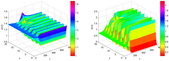
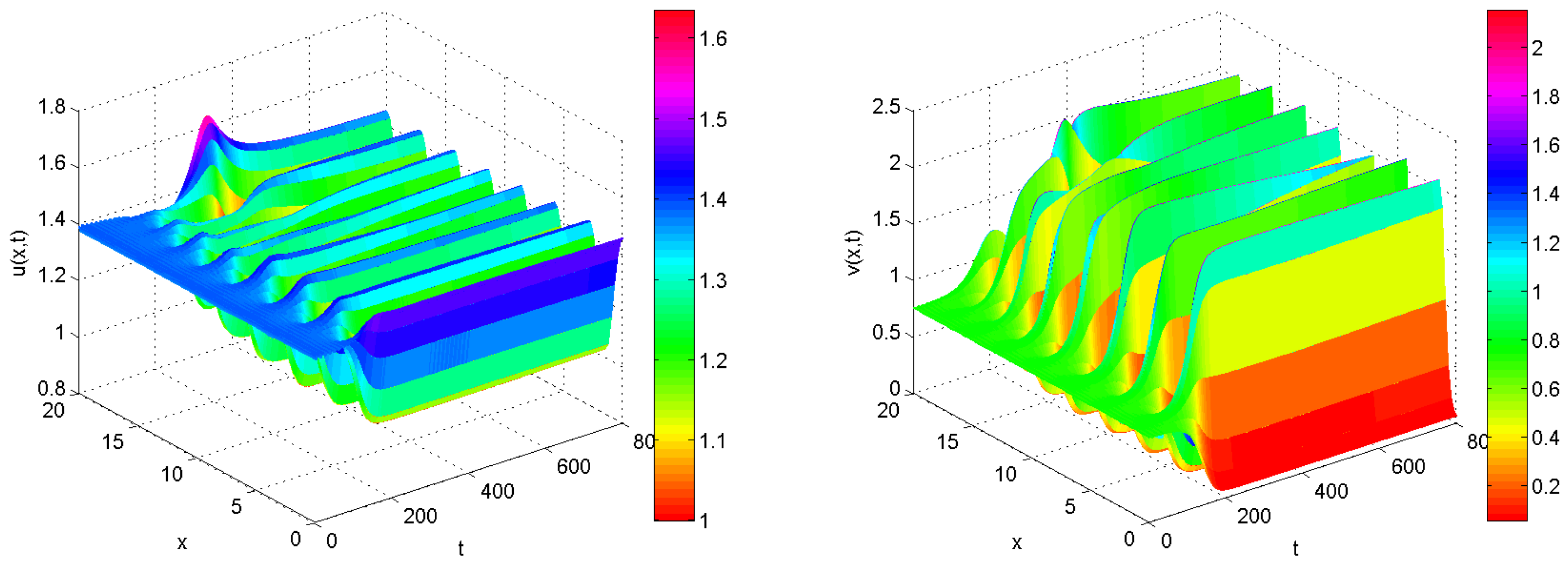
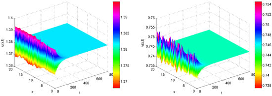
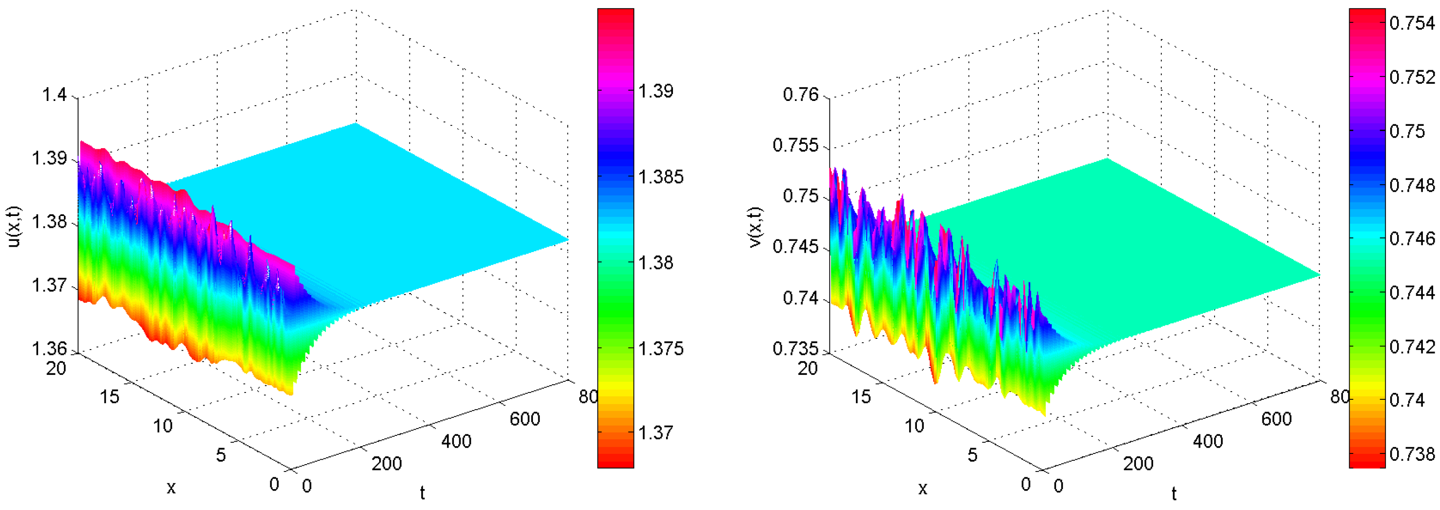
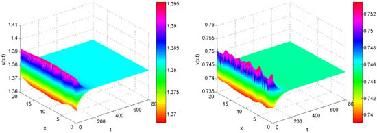
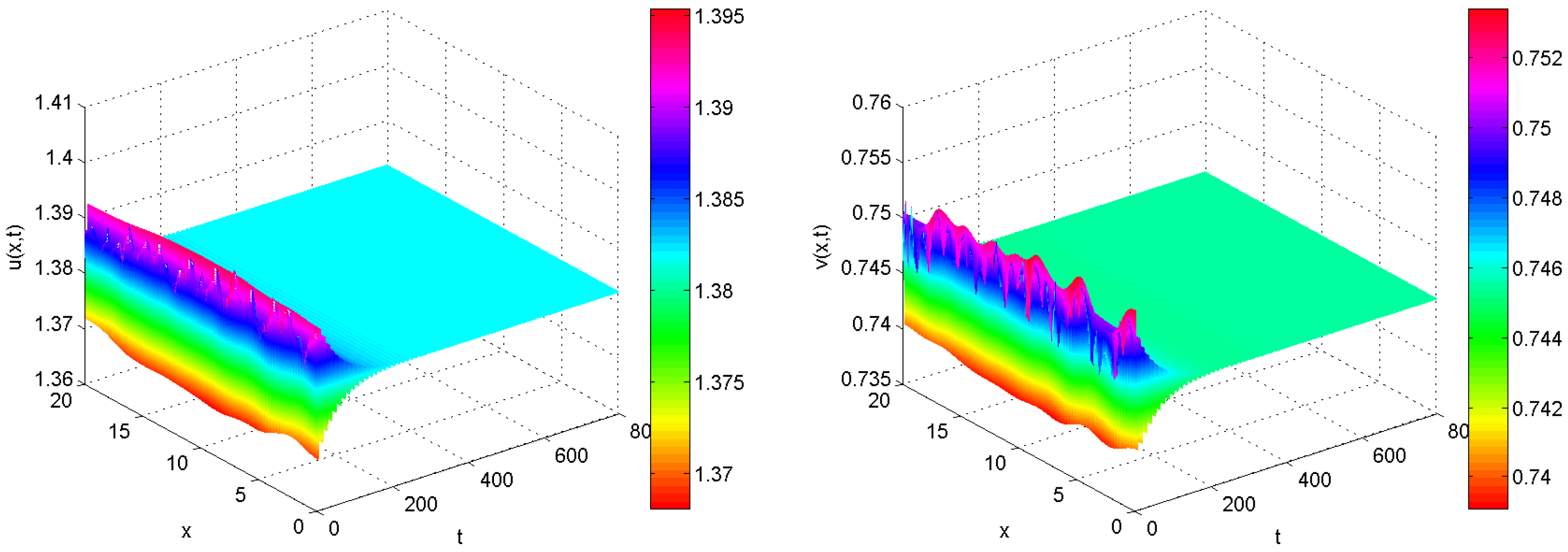
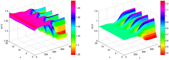
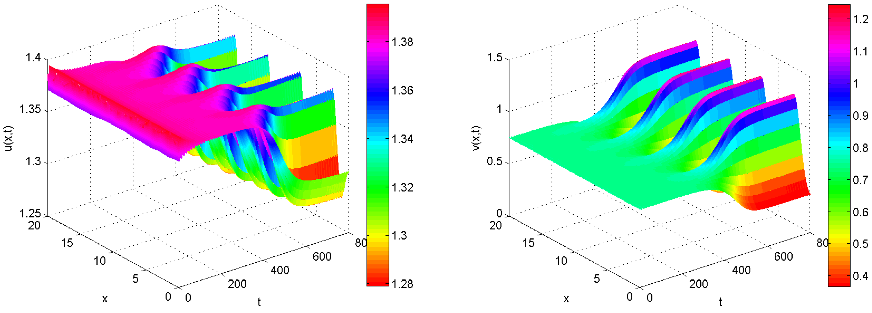
It is evident that model (23) possesses a trivial equilibrium $E_0=(0,0)$, a boundary equilibrium $E_1=(3,0)$, and a unique positive equilibrium $E^{*}=(1.382,0.745)$. Note that under the given parameters (26), both conditions $\left(H_0\right)$ and $\left(H_1\right)$ are satisfied, rendering $E^{*}$ stable with respect to the corresponding ODE model (i.e., $d_1=d_2=\mathit{\chi }=0$). When we choose $d_2=0.01$, the equilibrium $E^{*}$ is unstable with respect to the corresponding reaction-diffusion model (see Figure 1), by performing calculations $\mathit{\chi }\left(k\right)=0.13$, taking $\mathit{\chi }=0.2>0.13$, $E^{*}$ is unstable with respect to model (23), which shows that positive predator-taxis have stabilizing effects (see Figure 2). When we choose $d_2=0.1$, $E^{*}$ is locally asymptotically stable with respect to the corresponding reaction-diffusion model (see Figure 3), the calculation gives that $\mathit{\chi }\left(k\right)=-0.537$, taking $\mathit{\chi }=-0.59<-0.537$, $E^{*}$ is stable with respect to the model (23), indicating that the negative predator-taxis have a destabilizing effect (see Figure 4).

Figure 1. When $d_2=0.01,\mathit{\chi }=0$, $E^{*}$ is unstable for model (23) with (26).

Figure 2. When $d_2=0.01,\mathit{\chi }=0.2>0.13$, $E^{*}$ is local asymptotically stable, which is caused by the predator-taxis for model (23) with (26).

Figure 3. When $d_2=0.1,\mathit{\chi }=0$, $E^{*}$ is local asymptotically stable for model (23) with (26).

Figure 4. When $d_2=0.1,\mathit{\chi }=-0.59<-0.537$, $E^{*}$ is unstable caused by the predator-taxis for model (23) with (26).

5. Concluding Remarks

This paper mainly discusses the dynamics of the predator-prey diffusion model with hunting cooperation and predator-taxis, where hunting cooperation refers to the cooperative behavior of some predator populations in the process of capturing prey. The predator-taxis effect refers to the response of prey to different predator distributions, i.e., the prey may move in the direction of a low predator gradient to avoid being captured by predators, or it may move in the direction of a high density of prey to defend against predator attacks. Hunting cooperation and predator-taxis have far-reaching implications for protecting endangered species and maintaining sustainable ecosystems.

Firstly, the global existence and uniform boundedness of a classical solution of the model are proven strictly. Secondly, the local stability of a positive equilibrium is discussed through linearization analysis. Finally, we use numerical simulations to visualize the results. In addition, it can be seen from [10] that the stability of the reaction-diffusion model depends on the ratio $d_1/d_2$ of diffusion coefficients. Combined with the discussion results of this paper, we found that in the same region, if this ratio is less than a critical value, it means that the predator occupies an advantageous position, which indicates that due to strong predation pressure, the prey should stay away from the predator’s habitat to avoid being predation. On the contrary, if this ratio is greater than a critical value, the situation is more favorable for the prey, which means that in the face of an attack by predators, the prey must collectively gather together and resist to obtain more survival opportunities, which is more conducive to the long-term development of the population.

References

- Scheel, D.; Packer, C. Group hunting behaviour of lions: A search for cooperation. Anim. Behav. 1991, 41, 697–709. [Google Scholar] [CrossRef] [Scilit]
- Boesch, C.; Boesch, H.; Vigilant, L. Cooperation in Primates and Humans: Mechanisms of Evolution; Kappeler, P.M., van Schaik, C.P., Eds.; Springer: New York, NY, USA, 2006. [Google Scholar]
- Cook, W.L.; Streams, F.A. Fish predation on Notonecta (Hemiptera): Relationship between prey risk and habitat utilization. Oecologia 1984, 64, 177–183. [Google Scholar] [CrossRef] [Scilit] [PubMed]
- Hector, D.P. Cooperative hunting and its relationship to foraging success and prey size in an avian predator. Ethology 1986, 73, 247–257. [Google Scholar] [CrossRef] [Scilit]
- Moffett, M.W. Foraging dynamics in the group-hunting myrmicine ant, pheidologeton diversus. J. Insect. Behav. 1988, 1, 309–331. [Google Scholar] [CrossRef] [Scilit]
- Goodale, E.; Beauchamp, G.; Ruxton, G.D. Mixed-Species Groups of Animals: Behavior, Community Structure, and Conservation; Academic Press: Cambridge, MA, USA, 2017. [Google Scholar]
- Duarte, J.; Januario, C.; Martins, N.; Sardanyes, J. Chaos and crises in a model for cooperative hunting: A symbolic dynamics approach. Chaos 2009, 19, 043102. [Google Scholar] [CrossRef] [Scilit]
- Berec, L. Impacts of foraging facilitation among predators on predator-prey dynamics. Bull. Math. Biol. 2010, 72, 94–121. [Google Scholar] [CrossRef] [Scilit] [PubMed]
- Alves, M.T.; Hilker, F.M. Hunting cooperation and Allee effects in predators. J. Theo. Biol. 2017, 419, 13–22. [Google Scholar] [CrossRef] [Scilit] [PubMed]
- Fu, S.M.; Zhang, H.S. Effect of hunting cooperation on the dynamic behavior for a diffusive Holling type II predator-prey model. Commun. Nonlinear Sci. Numer. Simulat. 2021, 99, 105807. [Google Scholar] [CrossRef] [Scilit]
- Kareiva, P.; Odell, G. Swarms of predators exhibit “preytaxis” if individual predators use area-restricted search. Am. Nat. 1987, 130, 233–270. [Google Scholar] [CrossRef] [Scilit]
- Jin, H.Y.; Wang, Z.A. Global stability of prey-taxis systems. J. Differ. Equ. 2017, 262, 1257–1290. [Google Scholar] [CrossRef] [Scilit]
- Choi, W.; Ahn, I. Predator invasion in predator-prey model with prey-taxis in spatially heterogeneous environment. Nonlinear Anal. Real World Appl. 2022, 65, 103495. [Google Scholar] [CrossRef] [Scilit]
- Zuo, W.J.; Song, Y.L. Stability and double-Hopf bifurcations of a Gause-Kolmogorov-type predator-prey system with indirect prey-taxis. J. Dyn. Diff. Equat. 2021, 33, 1917–1957. [Google Scholar] [CrossRef] [Scilit]
- Banda, H.; Chapwanya, M.; Dummani, P. Pattern formation in the Holling-Tanner predator-prey model with predator-taxis. A nonstandard finite difference approach. Math. Compu. Simul. 2022, 196, 336–353. [Google Scholar] [CrossRef] [Scilit]
- Chen, M.X.; Zheng, Q.Q. Predator-taxis creates spatial pattern of a predator-prey model. Chaos Solitons Fractals 2022, 161, 112332. [Google Scholar] [CrossRef] [Scilit]
- Gao, X.Y. Global solution and spatial patterns for a ratio-dependent predator-prey model with predator-taxis. Results Math. 2022, 77, 66. [Google Scholar] [CrossRef] [Scilit]
- Amann, H. Dynamic theory of quasilinear parabolic equations. II. Reaction-diffusion systems. Differ. Integral Equ. 1990, 3, 13–75. [Google Scholar] [CrossRef] [Scilit]
- Amann, H. Nonhomogeneous linear and quasilinear elliptic and parabolic boundary value problems. In Function Spaces, Differential Operators and Nonlinear Analysis; Teubner–Taxte Math: Stuttgart, Germany, 1993; Volume 133, pp. 9–126. [Google Scholar]
- Alikakos, N.D. Lp bounds of solutions of reaction-diffusion equations. Commun. Part. Diff. Equ. 1979, 4, 827–868. [Google Scholar] [CrossRef] [Scilit]
- Horstmann, D.; Winkler, M. Boundedness vs. blow-up in a chemotaxis system. J. Differ. Equ. 2005, 215, 52–107. [Google Scholar] [CrossRef] [Scilit]
- Friedman, A. Patial Differential Equations; Holt Rinehart Winston: New York, NY, USA, 1969. [Google Scholar]
- Burnside, W.S.; Panton, A.W. The Theory of Equations: With an Introduction to the Theory of Binary Algebraic Forms, 2nd ed.; Dublin University Press Series: Dublin, Ireland, 1886. [Google Scholar]
Disclaimer/Publisher’s Note: The statements, opinions and data contained in all publications are solely those of the individual author(s) and contributor(s) and not of MDPI and/or the editor(s). MDPI and/or the editor(s) disclaim responsibility for any injury to people or property resulting from any ideas, methods, instructions or products referred to in the content. |
© 2024 by the author. Licensee MDPI, Basel, Switzerland. This article is an open access article distributed under the terms and conditions of the Creative Commons Attribution (CC BY) license (https://creativecommons.org/licenses/by/4.0/).