A Novel Black-Litterman Model with Time-Varying Covariance for Optimal Asset Allocation of Pension Funds

Abstract

The allocation of pension funds has important theoretical value and practical significance, which improves the level of pension investment income, achieves the maintenance and appreciation of pension funds, and resolves the pension payment risk caused by population aging. The asset allocation of pension funds is a long-term asset allocation problem. Thus, the long-term risk and return of the assets need to be estimated. The covariance matrix is usually adopted to measure the risk of the assets, while calculating the long-term covariance matrix is extremely difficult. Direct calculations suffer from the insufficiency of historical data, and indirect calculations accumulate short-term covariance, which suffers from the dynamic changes of the covariance matrix. Since the returns of main assets are highly autocorrelated, the covariance matrix of main asset returns is time-varying with dramatic dynamic changes, and the errors of indirect calculation cannot be ignored. In this paper, we propose a novel Black–Litterman model with time-varying covariance (TVC-BL) for the optimal asset allocation of pension funds to address the time-varying nature of asset returns and risks. Firstly, the return on assets (ROA) and the covariance of ROA are modeled by VARMA and GARCH, respectively. Secondly, the time-varying covariance estimation of ROA is obtained by introducing an effective transformation of the covariance matrix from short-term to long-term. Finally, the asset allocation decision of pension funds is achieved by the TVC-BL model. The results indicate that the proposed TVC-BL pension asset allocation model outperforms the traditional BL model. When the risk aversion coefficient is 1, 1.5, and 3, the Sharp ratio of pension asset allocation through the TVC-BL pension asset allocation model is 13.0%, 10.5%, and 12.8% higher than that of the traditional BL model. It helps to improve the long-term investment returns of pension funds, realize the preservation and appreciation of pension funds, and resolve the pension payment risks caused by the aging of the population.

1. Introduction

Pensions, or pension insurance funds, are the most important component of the social pension security system. Due to the severe population aging and social, economic, and historical factors, the Chinese pension insurance system has been facing severe difficulties in pension disbursement [1,2]. Pensions also have the characteristics of long saving times and large capital scale. Therefore, it is urgent to make scientific and reasonable investment decisions, effectively prevent investment risks, and improve the return level. Asset allocation is the core of pension investment management and is the decisive factor in long-term pension returns and risks.

Asset allocation is an important part of the investment decision, where the investor usually selects the proper assets to be first allocated, followed by a secondary allocation within each asset class. In the practice of investment allocation, investors classify asset allocation according to different criteria. Strategic asset allocation and tactical asset allocation are divided based on functional differences. Strategic asset allocation is a method set by an investor with a long-term investment objective. It focuses on asset allocation for long-term investments, which can span as long as 5–10 years or even longer. Tactic asset allocation is a plan developed by an investor during strategic asset allocation. It focuses on the specific state and trends of the economy and markets, consistently functioning around strategic asset allocation [3,4,5,6]. The pension system in China is based on a pay-as-you-go method with long funding terms and weak risk tolerance. There are two distinctive features of pension investment management: one is the long-term investment method, with the fundamental goal of achieving stable and better long-term returns; the other is the diversified investment method.

For long-term asset allocation, the long-term risk and return of the assets need to be estimated. Since the returns of main assets are highly autocorrelated (especially those of monetary assets and bonds), the covariance matrix of asset returns is time-varying with dynamic changes [7,8,9]. In most existing studies, the multi-period covariance matrix is calculated by directly modeling the monthly data to obtain the monthly covariance matrix. Afterward, the covariance matrix of the other terms can be obtained by accumulating the monthly covariance matrices. For example, the monthly covariance matrix can be multiplied by 12 to obtain the annual covariance matrix [10,11]. However, this traditional calculation method assumes that the monthly covariance matrix will be constant in the future. For short-term asset allocation, this method has little impact on risk estimation. For long-term asset allocation, the long-term covariance matrix obtained by accumulating monthly covariance matrices causes inaccurate risk estimation due to the intrinsic link between short-term and long-term risks being neglected. Therefore, how to transform the short-term covariance matrix into a long-term covariance matrix by considering the asset autocorrelation needs to be investigated.

The allocation of pension funds is a long-term asset allocation problem. As a result, directly calculating the long-term covariance matrix suffers from problems such as insufficient historical data, and the intrinsic link between short-term and long-term risks might be neglected. Therefore, the long-term covariance matrix usually needs to be obtained by transforming the short-term covariance matrix. The traditional simple transformation approach ignores the autocorrelation of main asset returns, causing errors in the long-term covariance.

In previous studies, the covariance matrix was considered constant in the long-term asset allocation, which neglects the time-varying nature of the covariance matrix. In this study, we develop an effective method to transform the short-term and long-term covariance matrix to address the dynamically changing nature of asset returns and risks. On this basis, we propose a novel Black–Litterman model with time-varying covariance (TVC-BL) for the optimal asset allocation of pension funds. The innovations of this paper are as follows:

• An efficient method for transforming the short-term covariance matrix to the long-term covariance matrix is given.
• The risk estimation in the BL model is improved, and the TVC-BL model is constructed and used in pension asset allocation decisions.
• The validity of the TVC-BL pension asset allocation model is verified through actual data.

The remaining sections are organized as follows: Section 2 reviews the related literature. Section 3 introduces the detail of the proposed model. Section 4 contains the experimental analysis. Section 5 presents the conclusions.

2. Related Literature

The groundbreaking study of asset allocation began with Markowiz’s portfolio selection theory, which proposed a bivariate analysis approach considering return and risk and created the mean-variance model [12,13]. By introducing risk-free assets, Tobin derived the combination of the capital market line and the cut point of the efficient frontier using the mean-variance model [14]. Based on these studies, Sharp, Lintner, and Mossin established the famous capital asset pricing model (CAPM) [15,16,17]. Black and Litterman developed the Black–Litterman (BL) model by integrating the mean-variance model and the CAPM and introducing the subjective view of investors [18,19]. The model adopted Bayesian analysis to estimate the implied risk premiums of assets from an equilibrium market portfolio. Then, a portfolio of investor views was added to derive the optimal allocation weights using an inverse optimization approach.

Asset allocation is the core of pension investment management and the main determinant of long-term benefits and risks of pension. Modern investment theory has laid a solid theoretical foundation for pension asset allocation, accelerated the development of pension asset allocation research, and accumulated many meaningful research results. Dutta et al. used a simple mean-variance model to analyze the risk aversion and return level of pension portfolios [20]. Parra et al. studied the optimal asset allocation of pensions by using a fuzzy multi-objective programming method considering the objectives and constraints of return, risk, and liquidity [21]. Booth and Yakoubov put multiple assets into the mean-variance model of pension investment for analysis and research [22]. Blake studied the investment strategy of enterprise annuity and pointed out that in the long-term investment income, compared with other dynamic strategies, the static strategy with a higher proportion of equity investment has more advantages [23]. Through the use of the VaR method, Steven and Vigna evaluated the portfolio risk and deduced the optimal asset allocation formula of pensions using a dynamic programming method [24]. Sherris outlined the framework and techniques that can be used to determine portfolio selection or asset allocation strategies appropriate for life insurance and pension funds in a multi-period framework [25]. Defau and Moore introduced alternative assets to study the diversified investment trend of pensions [26]. In recent years, many scholars have studied and discussed the problem of the optimal management of pension funds [27,28,29].

The BL model has been widely used in practical allocations. Bevan and Winkelmann applied the BL model to the asset allocation process of Goldman Sachs and presented details such as model calibration [30]. To facilitate investors to express their views regarding volatility and correlation coefficients, Qian and Gorman suggested using conditional estimation methods to estimate the covariance matrix [31]. Many scholars used GARCH models to form investor views [32,33,34,35]. Martellini and Zieman investigated how to apply the BL model to the allocation of hedge funds [36]. Numerous studies have made extensions to the BL model. Cheung combined the BL model with factor analysis and proposed an augmented BL model [37]. O’Toole tried to explain the BL model using the risk budgeting approach in active management [38]. In recent years, many scholars have used the BL model to study pension investment. Miťková and Mlynarovič studied the performance and risk analysis of private pension funds in the Slovak Republic based on the BL model [39]. Park et al. explored a method to construct an optimal alternative portfolio for Korean NPF using the Markowitz mean-variance model and the BL model [40]. Platanakis and Sutcliffe used robust optimization techniques to solve the asset liability management (ALM) problem for pension plans [41]. A comparative analysis of asset allocation performance with the BL model was also performed. Buriticá-Mejía developed an efficient portfolio and frontier for the Colombian Mandatory Pension Funds using support-vector machines and BL models [42]. The results showed that by improving the prior distribution matrix, especially using support-vector regression, the model had a better-diversified portfolio compared to the Markowitz model. In addition, scholars such as Stoilov, Simos, and Barua also incorporated the new subjective view of investors into the BL model [43,44,45]. The BL model was improved from different perspectives by considering the transaction cost and the base constraint. The obtained portfolios exhibited considerable advantages over all benchmark model portfolios. However, research on improving risk estimation was still lacking.

Asset allocation aims to combine an investor’s risk appetite to maximize returns within certain risk constraints. Researchers revealed that risk estimation has a relatively large impact on asset allocation. Most existing studies on risk estimation for major asset classes are still based on sample covariance matrices [46]. However, as described by Ankrim, Fox, and Hensel, the covariance matrix of the sample is valid only if the returns obey a normal distribution with constant mean and constant variance [47]. Due to autocorrelation in broad asset class returns [7], using a sample covariance matrix in short-term asset allocation may ignore the time-varying nature of short-term volatility. If the matrix is transformed to a long-term covariance matrix, the dynamic characteristics of the covariance matrix with term could also be ignored, which further increases the error. In recent years, scholars (e.g., Ding and Martin; Cong and Oosterlee) have applied GARCH models to investigate investment management [48,49,50,51,52]. Although the GARCH model in short-term asset allocation considers the time-varying nature of volatility, its direct and simple transformation to long-term ignores the dynamic characteristics of the covariance matrix over time, making this method questionable.

According to the above literature analysis, asset allocation has a solid theoretical foundation in finance. It takes modern portfolio theory as the classical theoretical framework and features rich research results of theoretical and methodological innovations. In the practical asset allocation of pension funds, a wealth of results has been achieved in practice-oriented research. However, there are fewer studies combining time-varying covariance with BL models for pension asset allocation, and further research is needed.

3. Model

This section focuses on how a TVC-BL pension asset allocation model considering time-varying covariance is constructed.

3.1. VARMA-GARCH Model

In this subsection, the VARMA-GARCH model is constructed by combining the VARMA model and the GARCH model. First, the VARMA-GARCH model was obtained by modeling the mean of return on assets (ROA) with the VARMA model and the variance of ROA with the GARCH model.

To obtain the covariance matrix of the assets, the forecast model of ROA needs to be first established. Considering the autocorrelation of ROA, the VARMA was used to model ROA, which captured the data generation process of ROA based on the guaranteed autocorrelation. For the covariance of ROA, the GARCH was used for modeling.

We make assumptions as follows:

1.

We denote $n$ assets in the market;

2.

$r_t$ is considered as a column vector of asset returns ($n\times 1$ dimension);

3.

The mean of $r_t$ is assumed to obey the VARMA;

4.

The residue of $r_t$ is assumed to obey a normal distribution and the GARCH;

5.

The residue of the return of different assets is independent.

The VARMA model is expressed as Equation (1), and the GARCH model is expressed as Equation (2):

$$r_t=c+{\displaystyle \sum _{i=1}^p{\varphi }_i{r}_{t-i}+u_t-}{\displaystyle \sum _{j=1}^q{\theta }_j{u}_{t-j}}$$

(1)

$$u_t\left|I_{t-1}\right.\sim N(0,{\Sigma }_t)$$

(2)

where ${\varphi }_i$ is the coefficient matrix ($n\times n$ dimension) of the historical data on ROA, $i=1,\cdots ,p$; ${\theta }_j$ is the coefficient matrix ($n\times n$ dimension) of the historical data of ROA residuals, $j=1,\cdots ,q$; $c$ is a vector of constant terms ($n\times 1$ dimension); $u_t$ is white noise ($n\times 1$ dimension) and $u_t$ satisfies $E_{t-1}(u_t)=0$, when $s\ne 0$, $E_{t-1}(u_t{u}_{t-s}{}^T)=0$, indicating that $u_t$ is a variable unaffected by past information; $I_{t-1}$ is the set of all information available at the end of the $t-1$ term; ${\Sigma }_t=E_{t-1}(u_t{u}_t{}^T)$ is the error covariance matrix, and ${\Sigma }_t$ may rely on past information.

3.2. BL Model

Based on the VARMA-GARCH model established above, the BL model was introduced to construct the BL asset allocation model based on VARMA-GARCH. The construction of this model includes the following steps:

Step 1. Mean and variance modeling: constructing the VARMA-GARCH model based on historical data.

Step 2. Long-term covariance calculation: the long-term covariance matrix is obtained by accumulating the short-term covariance matrix.

Step 3. Equilibrium return calculation: performing inverse optimization based on the mean and variance models to obtain market equilibrium returns.

Step 4. Investor view construction: constructing investor views based on the forecasted asset returns.

Step 5. Posteriori estimate calculation: generating new estimates of return and covariance matrix through the BL model based on market equilibrium returns and investor views.

Step 6. Asset allocation decisions: making asset allocation decisions based on the mean and variance models.

The specific calculations for each step are as follows:

Step 1. Mean and variance modeling:

We considered three major asset classes, namely, stock, bond, and monetary assets. Let $r_t$ be the column vector of ROA, and the mean and variance of $r_t$ were modeled using the VARMA and GARCH models, see Equations (1) and (2), respectively.

The VARMA-GARCH model was employed to generate forecasts of the ROA, and the results were used in later steps.

Step 2. Long-term covariance calculation:

We assumed that the covariance matrix for each term ahead was constant. The covariance matrix for one term ahead was forecasted using the VARMA-GARCH model, and the cumulative covariance matrix for $m$ terms ahead was calculated as follows:

$${\sum }_t(m)=m{\sum }_{t+1}$$

(3)

where ${\sum }_t(m)$ is the cumulative return covariance matrix for the $m$ terms ahead, and ${\sum }_{t+1}$ is the covariance matrix for one term ahead.

Step 3. Equilibrium return calculation:

We assumed that the utility function of the investor is:

$$U=w^T\mathsf{\Pi }-\delta w^T\Sigma w$$

(4)

Through inverse optimization, the equilibrium rate of return was calculated by backward derivation based on the asset portfolio weights for the current equilibrium. We then took the derivative on both sides of Equation (4) and made it equal to 0:

$$\frac{dU}{dw}=\mathsf{\Pi }-2\delta \Sigma w_{mkt}=0$$

(5)

Further,

$$\mathsf{\Pi }=2\delta \Sigma w_{mkt}$$

(6)

where $\mathsf{\Pi }$ is the equilibrium return of the asset; $\Sigma ={\Sigma }_t(m)$ is the cumulative return covariance matrix for the $m$ terms ahead; $w_{mkt}$ is the equilibrium rate of return asset portfolio weight vector; and $\delta$ is the risk aversion coefficient.

Step 4. Investor view construction:

Based on the rolling forecast method, the returns of the $1,2,\cdots ,m$ terms ahead were forecasted using the VARMA-GARCH model, and the cumulative return of the $m$ term ahead was calculated using the following method:

$${\widehat{r}}_t^i(m)=\left(1+{\widehat{r}}_{t+1}^i\right)\left(1+{\widehat{r}}_{t+2}^i\right)\cdots \left(1+{\widehat{r}}_{t+m}^i\right)-1$$

(7)

where ${\widehat{r}}_t^i(m)$ is the cumulative return of the asset $i$ in the $m$ terms ahead; ${\widehat{r}}_{t+1}^i,{\widehat{r}}_{t+2}^i,\cdots ,{\widehat{r}}_{t+m}^i$ are the returns of the asset $i$ in the $1,2,\cdots ,m$ term ahead.

Based on the forecasted returns, the investor view matrix can be constructed as follows:

$$\begin{gathered} P=I=\left[\begin{array}{cccc}1& 0& \cdots & 0\\ 0& 1& \cdots & 0\\ ⋮& ⋮& \ddots & ⋮\\ 0& 0& \cdots & 1\end{array}\right] \\ Q={\widehat{r}}_t(m) \\ \mathsf{\Omega }={\sum }_t(m) \end{gathered}$$

(8)

where $P$ is the investor view matrix; $Q$ is the investor view return vector; and $\mathsf{\Omega }$ is the covariance matrix of view errors.

Step 5. Posteriori estimate calculation:

After adding the investor views to the prior distribution of asset returns, the newly synthesized return and covariance matrix can be derived by Bayesian methods as follows:

$${\mu }^{BL}={[{(\tau \Sigma )}^{-1}+P^T{\mathsf{\Omega }}^{-1}P]}^{-1}[{(\tau \Sigma )}^{-1}\mathsf{\Pi }+P^T{\mathsf{\Omega }}^{-1}Q]$$

(9)

$${\Sigma }^{BL}={[{(\tau \Sigma )}^{-1}+P^T{\mathsf{\Omega }}^{-1}P]}^{-1}$$

(10)

where ${\mu }^{BL}$ is the newly synthesized rate of return; ${\Sigma }^{BL}$ is the covariance matrix of $n$ assets; $\mathsf{\Pi }$ is the equilibrium return of assets; $\Sigma ={\Sigma }_t(m)$ is the cumulative return covariance matrix of the $m$ terms ahead; $\tau$ denotes the proportion of the equilibrium rate of the return covariance matrix to the actual covariance matrix; $Q$ is the investor view return vector; $P$ is the investor view matrix; and $\mathsf{\Omega }$ is the covariance matrix of view errors.

Step 6. Asset allocation decisions:

The newly synthesized rate of return ${\mu }^{BL}$ and covariance matrix ${\Sigma }^{BL}$ were brought back into the Markowitz mean-variance model below to generate the asset portfolio decision:

$$\underset{w}{\max }{w}^T\mathsf{\Pi }-\delta w^T\Sigma w$$

(11)

where $\delta$ is the risk aversion coefficient.

3.3. Derivation of the Time-Varying Covariance Matrix

In this section, the time-varying covariance matrix is further derived based on the VARMA-GARCH model to obtain the relationship between the covariance matrices at different terms.

By taking the unconditional expectation for both sides of Equation (1), the following equation can be obtained:

$$\left(I-{\displaystyle \sum _{i=1}^p{\varphi }_i}\right)r=c$$

(12)

where $r$ is the unconditional expectation of $r_t$; $I$ is the unit matrix of $n\times n$.

By substituting Equation (12) into Equation (1), the following equation can be obtained:

$$r_t-r={\displaystyle \sum _{i=1}^p{\varphi }_i(r_{t-i}-r)+u_t-}{\displaystyle \sum _{j=1}^q{\theta }_j{u}_{t-j}}$$

(13)

Equation (13) can be expressed by the lag operator as follows:

$$\varphi (L)(r_t-r)=\theta (L)u_t$$

(14)

where $\varphi (L)=I-{\varphi }_{1}L-\cdots -{\varphi }_p{L}^p$, $\theta (L)=I-{\theta }_{1}L-\cdots -{\theta }_q{L}^q$, and $L$ are the lag operators.

Based on Equation (14), the following equation can be further obtained:

$$r_t-r=\psi (L)u_t$$

(15)

where $\psi (L)=\varphi {(L)}^{-1}\theta (L)$.

According to the study of Dufour et al. [52], it can be obtained that $\psi (L)=I-{\displaystyle \sum _{j=1}^{\infty }{\psi }_j{L}^j}$.

By substituting Equation (12) into Equation (1), the following equation can be obtained:

$$r_t-r=(I-{\displaystyle \sum _{j=1}^{\infty }{\psi }_j{L}^j)u_t}=u_t-{\displaystyle \sum _{j=1}^{\infty }{\psi }_j{L}^j{u}_t}=u_t-{\displaystyle \sum _{j=1}^{\infty }{\psi }_j{u}_{t-j}}$$

(16)

Based on the above analysis, we obtained a new equation for $r_t$.

Further, the unconditional self-covariance of $r_t$ can be calculated according to Equation (16):

$$\begin{gathered} {\Gamma }_r(h)=E\left\{(r_t-r){(r_{t-h}-r)}^T)\right\} \\ =E\{(u_t-{\displaystyle \sum _{j=1}^{\infty }{\psi }_j{u}_{t-j})}(u_{t-h}-{\displaystyle \sum _{j=1}^{\infty }{\psi }_j{u}_{t-h-j}{)}^T}\} \\ \begin{array}{l}=E\left\{\left[u_t\right]{\left[{\psi }_h{u}_t\right]}^T\right\}+E\left\{\left[{\psi }_1{u}_{t-1}\right]{\left[{\psi }_{h+1}{u}_{t-1}\right]}^T\right\}+\\ \\ +E\left\{\left[{\psi }_2{u}_{t-2}\right]{\left[{\psi }_{h+2}{u}_{t-2}\right]}^T\right\}+\cdots \end{array} \\ ={\displaystyle \sum _{j=0}^{\infty }{\psi }_{h+j}\Sigma {\psi }_j{}^T} \end{gathered}$$

(17)

where $\Sigma =E(u_t{u}_t{}^T)$ is the unconditional covariance matrix of the white noise $u_t$.

In Equation (17), ${\psi }_j$ is the parameter set to obtain the relationship between $r_t$ and $u_t$. The value of ${\psi }_j$ is related to ${\varphi }_i$ and ${\theta }_j$, but the exact relationship is not given. The equation for ${\psi }_j$ is derived below.

Since $\psi (L)=\varphi {(L)}^{-1}\theta (L)=I-{\displaystyle \sum _{j=1}^{\infty }{\psi }_j{L}^j}$, which means $\varphi (L)\psi (L)=\theta (L)$, the following equation can be obtained:

$$(I-{\displaystyle \sum _{i=1}^p{\varphi }_i{L}^i)(}I-{\displaystyle \sum _{j=1}^{\infty }{\psi }_j{L}^j})=(I-{\displaystyle \sum _{j=1}^q{\theta }_j{L}^j})$$

(18)

After expanding Equation (18), it can be obtained that:

$$I-{\displaystyle \sum _{j=1}^{\infty }{\psi }_j{L}^j}-{\displaystyle \sum _{i=1}^p{\varphi }_i{L}^i+}{\displaystyle \sum _{i=1}^p{\varphi }_i{L}^i\cdot }{\displaystyle \sum _{j=1}^{\infty }{\psi }_j{L}^j}=I-{\displaystyle \sum _{j=1}^q{\theta }_j{L}^j}$$

(19)

By simplifying Equation (19), it can be obtained that:

$${\displaystyle \sum _{j=1}^q{\theta }_j{L}^j}-{\displaystyle \sum _{j=1}^{\infty }{\psi }_j{L}^j}-{\displaystyle \sum _{i=1}^p{\varphi }_i{L}^i+}{\displaystyle \sum _{i=1}^p{\varphi }_i{L}^i\cdot }{\displaystyle \sum _{j=1}^{\infty }{\psi }_j{L}^j}=0$$

(20)

Based on the above equations, the following equations can be obtained:

$$\begin{gathered} {\psi }_1={\theta }_1-{\varphi }_1, \\ {\psi }_j={\theta }_j-{\varphi }_j+{\displaystyle \sum _{i=1}^{j-1}{\varphi }_i{\psi }_{j-i}} \end{gathered}$$

(21)

where ${\theta }_j=0$ when $j>q$; ${\varphi }_j=0$ when $j>p$.

In summary, ${\psi }_j$ can be calculated using the following recursive equations:

$$\begin{gathered} {\psi }_0=I, \\ {\psi }_1={\theta }_1-{\varphi }_1, \\ {\psi }_j={\theta }_j-{\varphi }_j+{\displaystyle \sum _{i=1}^{j-1}{\varphi }_i{\psi }_{j-i}}, \end{gathered}$$

(22)

where ${\theta }_j=0$ when $j>q$; ${\varphi }_j=0$ when $j>p$.

The asset allocation of pension funds usually requires a long decision time. Taking the annual asset allocation decision as an example, the covariance matrix was first modeled with monthly data to estimate the covariance matrix for the coming month. However, for asset allocation, the covariance matrix for the next year (the cumulative covariance matrix for the next 12 months) needs to be obtained. Therefore, the quantitative relationship between the covariance matrix of a coming term and the cumulative covariance matrices of multiple future terms needs to be obtained. We first derived the covariance matrix of the $h$th term ahead. On this basis, the cumulative covariance matrix for $m$ terms ahead was derived.

The covariance matrix of the h th term ahead

Assuming that $r_t$ undergoes the VARMA process, the forecasted return of 1 term ahead is

$${\widehat{r}}_{t+1}={\displaystyle \sum _{i=0}^{p-1}{\varphi }_{i+1}{r}_{t-i}-}{\displaystyle \sum _{j=0}^{q-1}{\theta }_{j+1}{u}_{t-j}}$$

(23)

The forecast error for the return of 1 term ahead is $u_{t+1}$.

The covariance matrix for the return of 1 term ahead is ${\sum }_{t+1}$.

By recursive calculation, we can obtain the forecasted return of the $h$th term ahead as

$${\widehat{r}}_{t+h}={\displaystyle \sum _{i=1-h}^{p-h}{\varphi }_{i+h}E(r_{t-i})-}{\displaystyle \sum _{j=1-h}^{q-h}{\theta }_{j+h}E(u_{t-j})}$$

(24)

where $E(r_{t-i})=\left\{\begin{array}{c}{r}_{t-i},i\ge 0\\ {\widehat{r}}_{t-i},i<0\end{array}\right.$, and $E(u_{t-j})=\left\{\begin{array}{c}{u}_{t-j},j\ge 0\\ {\widehat{u}}_{t-j},j<0\end{array}\right.$.

When performing multi-step forecasting, the forecasted value of the previous step needs to be brought into Equation (24) for the forecast of the next step. Therefore, the forecast errors before the $h$th term are accumulated into the forecast error for the $h$th term. That is, all forecast errors up to the $h$th term need to be considered when calculating the covariance matrix for the returns of the $h$th term ahead.

Based on the previously derived Equation (16), the formula for $r_{t+h}$ can be obtained as follows:

$$r_{t+h}-E(r_{t+h})=\left\{\begin{array}{c}{u}_{t+h}, h=1\\ u_{t+h}-{\displaystyle \sum _{j=1}^{h-1}{\psi }_j{u}_{t-j+h}}, h\ge 2\end{array}\right.$$

(25)

According to Equation (25), the formula for $r_{t+h}$ changes depending on $h$. Therefore, we analyze the covariance matrix for the $h$th term ahead in two scenarios.

When $h=1$, the covariance matrix for the $h$th term ahead is calculated as follows:

$$\begin{array}{ll}{\sum }_{t,h}& =E\left\{\left[r_{t+h}-E(r_{t+h})\right]{\left[r_{t+h}-E(r_{t+h})\right]}^T\right\}\\ & =E\left\{\left[u_{t+h}\right]{\left[u_{t+h}\right]}^T\right\}\\ & ={\Sigma }_{t+h}\end{array}$$

(26)

When $h\ge 2$, the covariance matrix for the $h$th term ahead is calculated as follows:

$$\begin{array}{l}{\sum }_{t,h}=E\left\{\left[r_{t+h}-E(r_{t+h})\right]{\left[r_{t+h}-E(r_{t+h})\right]}^T\right\}\\ =E\left\{\left[u_{t+h}-{\displaystyle \sum _{j=1}^{h-1}{\psi }_j{u}_{t-j+h}}\right]{\left[u_{t+h}-{\displaystyle \sum _{j=1}^{h-1}{\psi }_j{u}_{t-j+h}}\right]}^T\right\}\\ =E\left\{\left[u_{t+h}\right]{\left[u_{t+h}\right]}^T\right\}+E\left\{\left[{\psi }_1{u}_{t+h-1}\right]{\left[{\psi }_1{u}_{t+h-1}\right]}^T\right\}+\dots \\ +E\left\{\left[{\psi }_{h-1}{u}_{t+1}\right]{\left[{\psi }_{h-1}{u}_{t+1}\right]}^T\right\}\\ ={\Sigma }_{t+h}+{\psi }_1{\Sigma }_{t+h-1}{\psi }_1{}^T+\dots +{\psi }_{h-1}{\Sigma }_{t+1}{\psi }_{h-1}{}^T\\ ={\psi }_0{\Sigma }_{t+h}{\psi }_0{}^T+{\psi }_1{\Sigma }_{t+h-1}{\psi }_1{}^T+\dots +{\psi }_{h-1}{\Sigma }_{t+1}{\psi }_{h-1}{}^T\\ ={\displaystyle \sum _{j=0}^{h-1}{\psi }_j{\Sigma }_{t+h-j}{\psi }_j{}^T}\end{array}$$

(27)

It is easy to verify that ${\sum }_{t,h}$ still satisfies Equation (27) when $h=1$, i.e.:

$$\begin{array}{l}{\sum }_{t,h}={\displaystyle \sum _{j=0}^{h-1}{\psi }_j{\Sigma }_{t+h-j}{\psi }_j{}^T}\\ ={\displaystyle \sum _{j=0}^0{\psi }_j{\Sigma }_{t+h-j}{\psi }_j{}^T}\\ ={\psi }_0{\Sigma }_{t+h}{\psi }_0{}^T\\ ={\Sigma }_{t+h}\end{array}$$

In summary, the covariance matrix for the $h$ term ahead is:

$${\sum }_{t,h}={\displaystyle \sum _{j=0}^{h-1}{\psi }_j{\Sigma }_{t+h-j}{\psi }_j{}^T}$$

(28)

The covariance matrix for the cumulative return of m terms ahead

Assuming that $r_{t,m}^{}$ is the cumulative return of $m$ terms ahead, we have:

$$r_{t,m}^{}=r_{t+1}+r_{t+2}+\dots +r_{t+m}$$

(29)

According to Equation (16) derived in the previous section, the formula for $r_{t,m}^{}$ can be obtained as follows:

$$r_{t,m}-E(r_{t,m})=\left\{\begin{array}{c}{u}_{t+1}, m=1\\ u_{t+1}+{\displaystyle \sum _{i=2}^m(u_{t+i}-{\displaystyle \sum _{j=1}^{i-1}{\psi }_j{u}_{t-j+i}})}, m\ge 2\end{array}\right.$$

(30)

where $r_{t+h}-E(r_{t+h})=\left\{\begin{array}{c}{u}_{t+h}, h=1\\ u_{t+h}-{\displaystyle \sum _{j=1}^{h-1}{\psi }_j{u}_{t-j+h}}, h\ge 2\end{array}\right.$.

According to Equation (30), the formula for $r_{t,m}^{}$ changes depending on $m$. Therefore, we analyze the covariance matrix for the cumulative return of $m$ terms ahead in two scenarios.

When $m=1$, the covariance matrix for the cumulative return of $m=1$ terms ahead can be calculated directly according to Equation (28).

$$\begin{array}{l}{\sum }_t(m)=E\left\{\left[r_{t,m}-E(r_{t,m})\right]{\left[r_{t,m}-E(r_{t,m})\right]}^T\right\}\\ =E\left\{\left[u_{t+1}\right]{\left[u_{t+1}\right]}^T\right\}\\ ={\Sigma }_{t+1}\end{array}$$

(31)

When $m\ge 2$, the covariance matrix for the cumulative return of $m$ terms ahead is calculated as follows:

$$\begin{array}{l}{\sum }_t(m)=E\left\{\left[r_{t,m}-E(r_{t,m})\right]{\left[r_{t,m}-E(r_{t,m})\right]}^T\right\}\cdots \\ =E\left\{\left[u_{t+1}+{\displaystyle \sum _{i=2}^m\left(u_{t+i}-{\displaystyle \sum _{j=1}^{i-1}{\psi }_j{u}_{t-j+i}}\right)}\right]{\left[u_{t+1}+{\displaystyle \sum _{i=2}^m\left(u_{t+i}-{\displaystyle \sum _{j=1}^{i-1}{\psi }_j{u}_{t-j+i}}\right)}\right]}^T\right\}\\ =E\left\{\left[\left({\displaystyle \sum _{j=1}^m{\psi }_{j-1}}\right)u_{t+1}+\left({\displaystyle \sum _{j=1}^m{\psi }_{j-2}}\right)u_{t+2}+\cdots +\left({\displaystyle \sum _{j=1}^m{\psi }_{j-m}}\right)u_{t+m}\right]\right.\\ \cdot \left.{\left[\left({\displaystyle \sum _{j=1}^m{\psi }_{j-1}}\right)u_{t+1}+\left({\displaystyle \sum _{j=1}^m{\psi }_{j-2}}\right)u_{t+2}+\cdots +\left({\displaystyle \sum _{j=1}^m{\psi }_{j-m}}\right)u_{t+m}\right]}^T\right\}\\ =E\left\{\left[{\displaystyle \sum _{i=1}^m\left({\displaystyle \sum _{j=1}^m{\psi }_{j-i}}\right)u_{t+i}}\right]{\left[{\displaystyle \sum _{i=1}^m\left({\displaystyle \sum _{j=1}^m{\psi }_{j-i}}\right)u_{t+i}}\right]}^T\right\}\\ ={\displaystyle \sum _{i=1}^m\left[\left({\displaystyle \sum _{j=1}^m{\psi }_{j-i}}\right)E\left(u_{t+i}\right)\right]{\left[\left({\displaystyle \sum _{j=1}^m{\psi }_{j-i}}\right)E\left(u_{t+i}\right)\right]}^T}\\ ={\displaystyle \sum _{i=1}^m\left[\left({\displaystyle \sum _{j=1}^m{\psi }_{j-i}}\right){\sum }_{t+i}{\left({\displaystyle \sum _{j=1}^m{\psi }_{j-i}}\right)}^T\right]}\end{array}$$

(32)

We can derive that Equation (32) still holds when $m=1$, i.e.,:

$$\begin{array}{ll}{\sum }_t(m)& ={\displaystyle \sum _{i=1}^m\left[\left({\displaystyle \sum _{j=1}^m{\psi }_{j-i}}\right){\sum }_{t+i}{\left({\displaystyle \sum _{j=1}^m{\psi }_{j-i}}\right)}^T\right]}\\ & ={\displaystyle \sum _{i=1}^1\left[\left({\displaystyle \sum _{j=1}^1{\psi }_{j-i}}\right){\sum }_{t+i}{\left({\displaystyle \sum _{j=1}^1{\psi }_{j-i}}\right)}^T\right]}\\ & ={\psi }_0{\sum }_{t+1}{\left({\psi }_0\right)}^T\\ & ={\sum }_{t+1}\end{array}$$

In summary, the covariance matrix for the cumulative return of $m$ terms ahead is:

$${\sum }_t(m)={\displaystyle \sum _{i=1}^m\left[\left({\displaystyle \sum _{j=1}^m{\psi }_{j-i}}\right){\sum }_{t+i}{\left({\displaystyle \sum _{j=1}^m{\psi }_{j-i}}\right)}^T\right]}$$

(33)

3.4. The Proposed TVC-BL Model

In the previous subsections, we first constructed the VARMA-GARCH model to capture the mean and variance of asset returns. Then, the VARMA-GARCH model and BL model were combined to produce a BL asset allocation model based on the VARMA-GARCH model. Finally, the calculation of time-varying covariance was provided based on the VARMA-GARCH model. Based on the findings in the previous sections, this subsection provides the modeling and solving steps of the TVC-BL pension asset allocation model.

The TVC-BL pension asset allocation model includes the following steps.

Step 1. Mean and variance modeling: constructing the VARMA-GARCH model based on historical data.

Step 2. Long-term covariance calculations: calculating the long-term covariance matrix based on the time-varying covariance formula.

Step 3. Equilibrium return calculation: performing inverse optimization based on the mean and variance models to obtain market equilibrium returns.

Step 4. Investor view construction: constructing investor views based on the forecasted asset returns.

Step 5. Posteriori estimate calculation: generating new estimates of return and covariance matrix through the BL model based on market equilibrium returns and investor views.

Step 6. Asset allocation decisions: making asset allocation decisions based on the mean and variance models.

The specific calculations for each step are as follows.

Step 1. Mean and variance modeling:

We considered three major asset classes, namely, stock, bond, and monetary assets. Let $r_t$ be the column vector of ROA; the mean and variance of $r_t$ were modeled using the VARMA and GARCH models, see Equations (1) and (2), respectively.

The VARMA-GARCH model was employed to generate forecasts of the ROAs, and the results were used in later steps.

Step 2. Long-term covariance calculations:

We assumed that the covariance matrix for each term ahead was time-varying. The covariance matrix for the $1,2,\cdots ,m$ terms ahead was forecasted using the VARMA-GARCH model, and the cumulative return covariance matrix for the $m$ terms ahead was further calculated as follows:

$${\sum }_t(m)={\displaystyle \sum _{i=1}^m\left[\left({\displaystyle \sum _{j=1}^m{\psi }_{j-i}}\right){\sum }_{t+i}{\left({\displaystyle \sum _{j=1}^m{\psi }_{j-i}}\right)}^T\right]}$$

(34)

where ${\sum }_t(m)$ is the cumulative return covariance matrix for the $m$ terms ahead, and ${\Sigma }_{t+1},{\Sigma }_{t+2},\cdots ,{\Sigma }_{t+m}$ is the covariance matrix for the $1,2,\cdots ,m$ term ahead.

Step 3. Equilibrium return calculation:

Assuming that the utility function of the investor is as Equation (4).

Through inverse optimization, the equilibrium rate of return was calculated by backward derivation based on the asset portfolio weights for the current equilibrium. See Equation (6).

Step 4. Investor view construction:

Based on the rolling forecast method, the returns of the $1,2,\cdots ,m$ terms ahead were forecasted using the VARMA-GARCH model, and the cumulative return of the $m$ term ahead was calculated using the following method:

$${\widehat{r}}_t^i(m)=\left(1+{\widehat{r}}_{t+1}^i\right)\left(1+{\widehat{r}}_{t+2}^i\right)\cdots \left(1+{\widehat{r}}_{t+m}^i\right)-1$$

(35)

where ${\widehat{r}}_t^i(m)$ is the cumulative return of asset $i$ in the $m$ terms ahead, and ${\widehat{r}}_{t+1}^i,{\widehat{r}}_{t+2}^i,\cdots ,{\widehat{r}}_{t+m}^i$ are the returns of asset $i$ in the $1,2,\cdots ,m$ term ahead.

Based on the forecasted returns, the investor view matrix can be constructed as follows:

$$\begin{gathered} P=I=\left[\begin{array}{cccc}1& 0& \cdots & 0\\ 0& 1& \cdots & 0\\ ⋮& ⋮& \ddots & ⋮\\ 0& 0& \cdots & 1\end{array}\right] \\ Q={\widehat{r}}_t(m) \end{gathered}$$

(36)

$$\mathsf{\Omega }={\sum }_t(m)$$

(37)

where $Q$ is the investor view return vector; $P$ is the investor view matrix; and $\mathsf{\Omega }$ is the covariance matrix of view errors.

Step 5. Posteriori estimate calculation:

After adding the investor views to the a priori distribution of asset returns, the newly synthesized return and covariance matrix can be derived by Bayesian methods as Equations (9) and (10).

Step 6. Asset allocation decisions:

The newly synthesized rate of return ${\mu }^{BL}$ and covariance matrix ${\Sigma }^{BL}$ were brought back into the Markowitz mean-variance model below to generate the asset portfolio decision. See Equation (11).

4. Experimental analysis

4.1. Data Selection and Description

The investment of pension funds is essentially a long-term asset allocation decision. Meanwhile, it is diversified. In addition to complying with national regulations, it follows the principle of safety first. Although China’s regulations on the investment management of pension funds have expanded the investment scope, the main investment categories of pension funds are currently dominated by stocks, equity, bonds, and cash. Despite their high risks, stocks can increase the level of long-term returns, making the stock market a very important investment channel for pension funds. Bonds, on the other hand, have relatively low returns and risks, thus satisfying the capital preservation, value preservation, and appreciation requirements of pension investments through stable returns. Cash has good liquidity. In addition, China’s relevant regulatory policies allow the conversion of a portion of assets into cash during pension investments without changing the total amount of pension assets. Thus, cash was considered as well [20].

We selected three major asset classes: stocks, bonds, and monetary assets. The CSI All Share Index, CSI All Bond Index, and CSI Monetary Fund Index were selected as the subject matter indexes for the three assets. The indexes were obtained from the Choice financial terminal, and the sample interval was monthly data from February 2005 to February 2021. The original data selected were the monthly closing prices of stocks, bonds, and monetary assets, which required preparatory processing.

The selection of basic data involved the monthly closing price of stocks, bonds, and monetary assets, so it was necessary to prepare the data. The monthly returns of each asset were calculated according to the price data of each asset. After obtaining the time series data of three types of asset returns, we carried out descriptive statistical analysis on the historical return data of three types of assets. The statistical analysis results are shown in Table 1.

Table 1. The descriptive statistical results of historical returns data of three types of assets.

	Stocks	Bonds	Cash
Index	CSI All Share Index	CSI All Bond Index	CSI Monetary Fund Index
Date sources	Choice	Choice	Choice
Sample interval	February 2005–February 2021	February 2005–February 2021	February 2005–February 2021
Sample size	194	194	194
Mean	1.295	0.373	0.251
Min	−25.910	−2.040	0.091
Max	29.535	4.124	0.538
Median	1.268	0.383	0.236
Variance	73.060	0.662	0.008
Skewness	1.133	3.563	−0.490
Kurtosis	−0.185	0.750	0.368

4.2. Time-Varying Properties of the Covariance Matrix

We calculated the covariance matrices for 1, 2, 3, 6, and 12 months from the historical data and transformed the sample covariance matrices for 1, 2, 3, and 6 months into a 12-month covariance matrix (annualized covariance matrix) by cumulative addition. The sample covariance matrices and annualized covariance matrices for stocks, bonds, and monetary assets at different terms are shown in Table 2. The annualized covariance matrices for stock, bond, and monetary assets are shown under different terms. Since the values in the covariance matrices were small, the data in Table 2 and Table 3 were the results of expanding the original data by a factor of 10,000.

Table 2. The sample covariance matrices of stock, bond, and monetary assets under different terms.

Covariance Matrix Entries	Investment Terms
	1 Month	2 Months	3 Months	6 Months	12 Months
Stock asset variance	73.439	178.483	318.448	908.031	2340.420
Bond asset variance	0.665	1.810	3.144	9.203	22.656
Monetary asset variance	0.008	0.028	0.062	0.242	0.866
Stock-bond asset covariance	−1.459	−5.486	−12.362	−41.173	−106.991
Stock-monetary asset covariance	−0.080	−0.401	−0.762	−3.940	−14.060
Bond-monetary asset covariance	0.011	0.035	0.056	0.270	0.711

Table 3. The annualized covariance matrices for stock, bond, and monetary assets under different terms.

Covariance Matrix Entries	Investment Terms
	1 Month	2 Months	3 Months	6 Months	12 Months
Stock asset variance	881.266	1070.898	1273.792	1816.062	2340.420
Bond asset variance	7.982	10.857	12.574	18.406	22.656
Monetary asset variance	0.094	0.170	0.247	0.484	0.866
Stock-bond asset covariance	−17.509	−32.918	−49.446	−82.347	−106.991
Stock-monetary asset covariance	−0.960	−2.407	−3.047	−7.880	−14.060
Bond-monetary asset covariance	0.137	0.211	0.225	0.539	0.711

According to Table 3, a comparison between the annualized covariance matrices obtained from the sample covariance matrices of different terms reveals that the sample variances of stocks, bonds, and monetary assets all gradually increase with the increase in investment term. Taken together, long-term covariance matrices based on the accumulation of short-term covariance matrices are underestimated due to the autocorrelation of the assets. That is, the risk calculated by direct accrual increases progressively as the investment term increases.

Considering the strong autocorrelation of major asset classes, the dynamic nature of the covariance matrix cannot be ignored in asset allocations. The traditional direct accumulation method ignores the dynamic nature of the covariance matrix, making the estimate of the covariance matrix lower than the actual value. Effectively transforming short-term covariance matrices into long-term covariance matrices has important implications for asset allocation.

4.3. Time-Varying Properties of the Covariance Matrix

Based on historical data on asset returns, the VARMA model was first constructed as Equation (1).

To identify the best VARMA ($p,q$) model, we based the model selection on the Akaike information criterion (AIC) and Bayesian information criterion (BIC).

By setting the range of $p$ and $q$ as {1, 2, 3, 4}, different VARMA ($p,q$) models were obtained.

The AIC and BIC of the VARMA models with different parameters were calculated, and the VARMA (1, 1) model was selected for the final VARMA model parameters based on the AIC and BIC minimization principles and the model fitting parameters.

Furthermore, the parameters obtained from the model are as follows.

The parameters of the VARMA (1, 1) model are as follows:

$$\begin{array}{r}\left[\begin{array}{c}{r}_{1t}\\ r_{2t}\\ r_{3t}\end{array}\right]=\left[\begin{array}{c}4.011\\ 0.115\\ 0.071\end{array}\right]+\left[\begin{array}{rrr}0.143& -1.047& -9.841\\ -0.033& 0.512& 0.441\\ -0.010& -0.061& 0.857\end{array}\right]\left[\begin{array}{c}{r}_{1t-1}\\ r_{2t-1}\\ r_{3t-1}\end{array}\right]\\ +\left[\begin{array}{rrr}-0.024& -0.637& 4.686\\ 0.024& -0.186& -1.461\\ 0.010& 0.061& -0.330\end{array}\right]\left[\begin{array}{c}{u}_{1t-1}\\ u_{2t-1}\\ u_{3t-1}\end{array}\right]+\left[\begin{array}{c}{u}_{1t}\\ u_{2t}\\ u_{3t}\end{array}\right]\end{array}$$

(38)

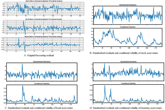
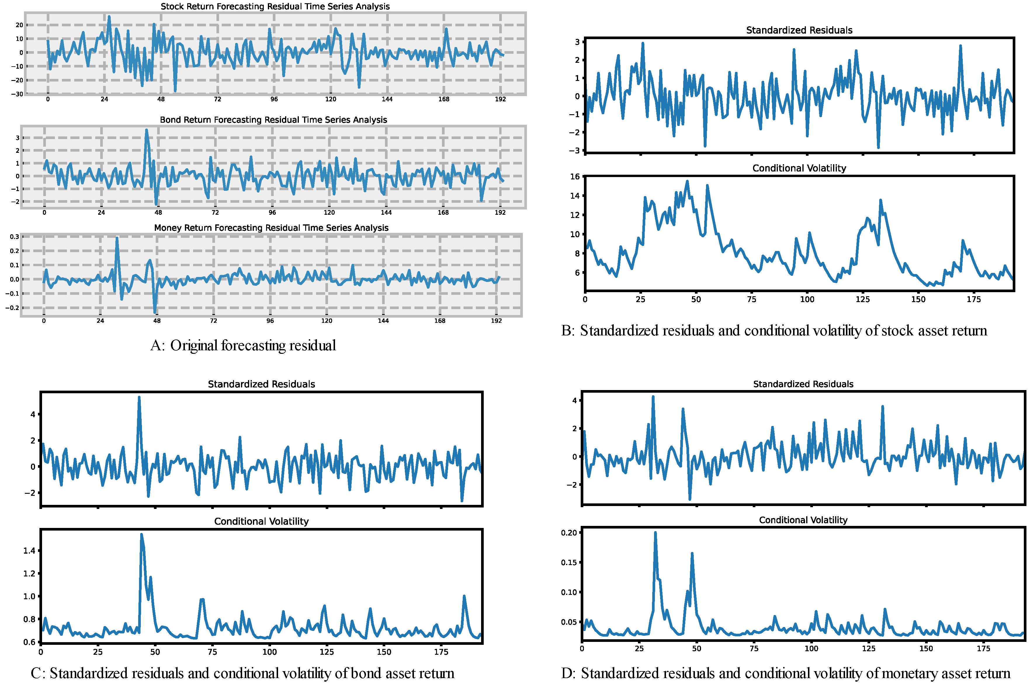
Based on the forecasts of the VARMA (1, 1) model, we obtained the time series of the residual for the three asset classes. The residual series of the three asset classes are shown in Figure 1A.

Figure 1. Asset return residual and conditional volatility.

Further, we constructed multivariate GARCH models for stocks, bonds, and monetary assets. The Constant Conditional Correlation GARCH (CCC-GARCH) model was adopted for modeling, which first estimated the variance of each asset before generating the multivariate GARCH model based on the correlation coefficients between each asset.

To determine the best GARCH model, the model selection was based on AIC and BIC. By setting the range of $p$ and $q$ as {1, 2, 3, 4}, different GARCH ($p,q$) models were obtained. By calculating the AIC and BIC of the GARCH model for each asset with different parameters, the optimal GARCH model for the stock residual series was selected as GARCH (1, 1). Similarly, we obtained the optimal GARCH model for the bond residual series as GARCH (1, 1) and the optimal GARCH model for the monetary asset residual series as GARCH (1, 1).

The estimated parameters of the GARCH (1, 1) model for the stock residual series are as follows:

$$h_{s,t}=3.678+0.188{\epsilon }_{s,t-1}^2+0.767h_{s,t-1}$$

(39)

where $h_{s,t}$ is the variance of stock assets in the term $t$, ${\epsilon }_{s,t-1}^2$ is the square of the residuals of stock assets returns in the term $t-1$ (ARCH term), and $h_{s,t-1}$ is the variance of stock assets in the term $t-1$ (GARCH term).

The estimated parameters of the GARCH (1, 1) model for the bond residual series are as follows:

$$h_{b,t}=0.228+0.149{\epsilon }_{b,t-1}^2+0.419h_{b,t-1}$$

(40)

where $h_{b,t}$ is the variance of bond assets in term $t$, ${\epsilon }_{b,t-1}^2$ is the square of the residuals of bond assets returns in term $t-1$ (ARCH term), and $h_{b,t-1}$ is the variance of bond assets in term $t-1$ (GARCH term).

The estimated parameters of the GARCH (1, 1) model for the monetary assets residual series are as follows:

$$h_{m,t}=0.001+0.452{\epsilon }_{m,t-1}^2+0.314h_{m,t-1}$$

(41)

where $h_{m,t}$ is the variance of monetary assets in term $t$, ${\epsilon }_{m,t-1}^2$ is the square of the residuals of monetary assets returns in term $t-1$ (ARCH term), and $h_{m,t-1}$ is the variance of monetary assets in term $t-1$ (GARCH term).

After obtaining the parameter estimates of the GARCH model for the different assets, we can calculate the covariance of the assets based on the correlation coefficients among them. The covariances among the different assets are calculated as follows:

$$\begin{gathered} h_{sb,t}={\rho }_{sb,t}\sqrt{h_{s,t}}\sqrt{h_{b,t}} \\ {h}_{sm,t}={\rho }_{sm,t}\sqrt{h_{s,t}}\sqrt{h_{m,t}} \\ {h}_{bm,t}={\rho }_{bm,t}\sqrt{h_{b,t}}\sqrt{h_{m,t}} \end{gathered}$$

(42)

where $h_{sb,t}$ is the covariance between stocks and bonds for the term $t$, $h_{sm,t}$ is the covariance between stocks and monetary assets for the term $t$, $h_{bm,t}$ is the covariance between bonds and monetary assets for the term $t$, ${\rho }_{sb}$ is the correlation coefficient between stocks and bonds, ${\rho }_{sm}$ is the covariance between stocks and monetary assets, and $h_{bm}$ is the covariance between bonds and monetary assets.

Based on the above calculations, we can obtain the final covariance matrix as follows:

$${\Sigma }_t=\left[\begin{array}{ccc}{h}_{s,t}& h_{sb,t}& h_{sm,t}\\ h_{sb,t}& h_{b,t}& h_{bm,t}\\ h_{sm,t}& h_{bm,t}& h_{m,t}\end{array}\right]$$

(43)

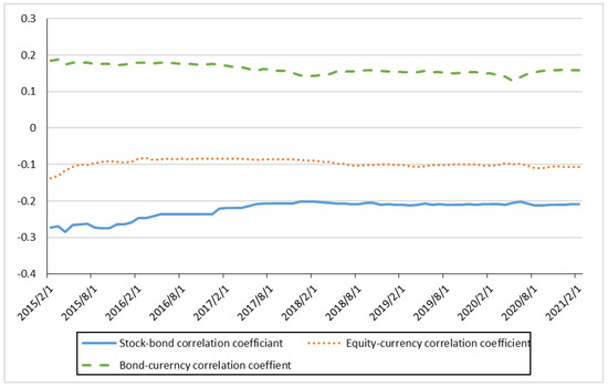
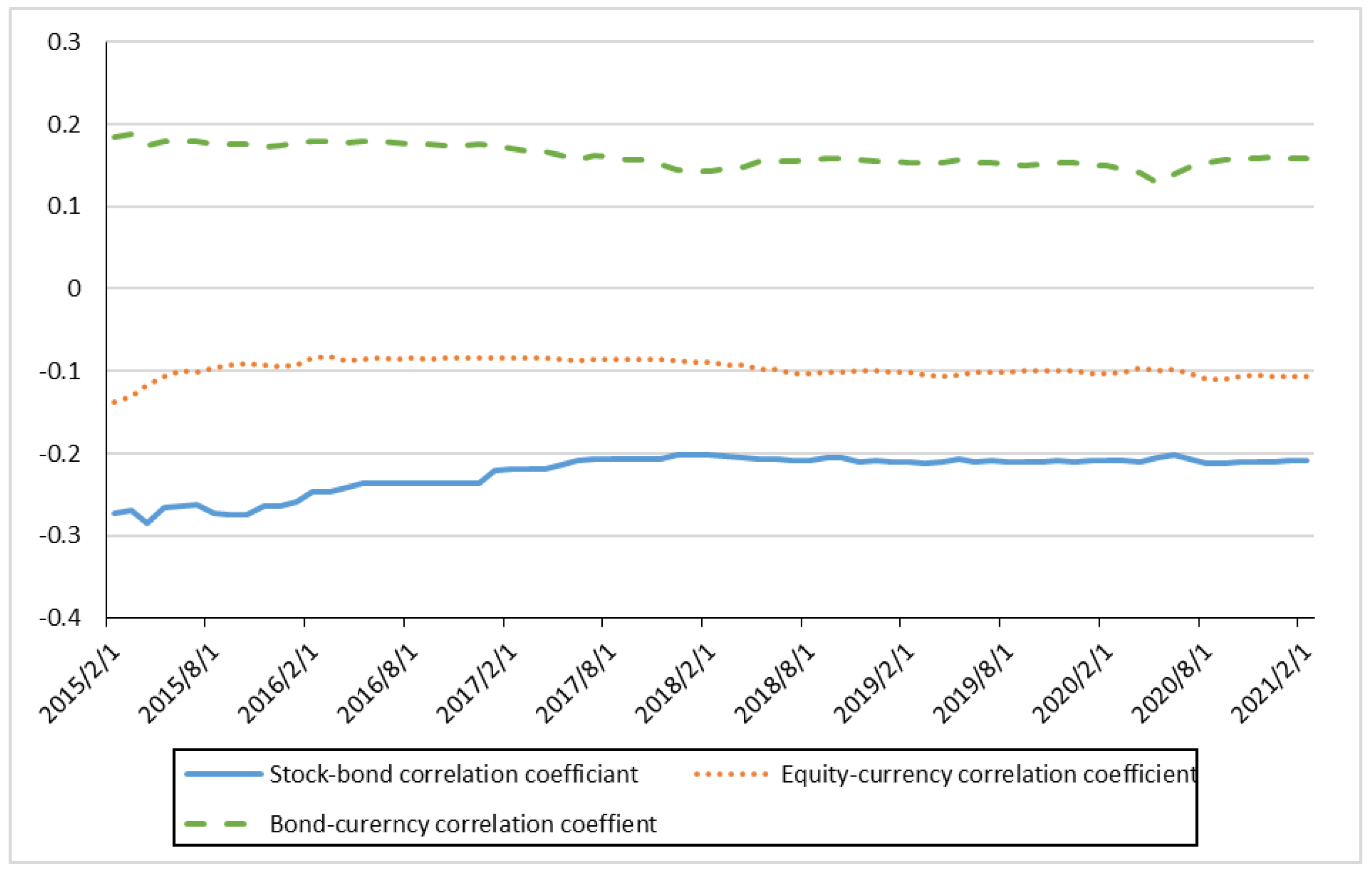
The correlation coefficient changes for the returns of the three asset classes, stocks, bonds, and monetary assets, are presented in Figure 2.

Figure 2. Correlation coefficient changes of the three types of assets.

4.4. Effectiveness Analysis for the TVC-BL Pension Asset Allocation Model

In this subsection, the proposed TVC-BL model considering the time-varying covariance was applied to pension asset allocation to further analyze its effectiveness in pension asset allocation.

In order to analyze the effectiveness of the proposed TVC-BL pension asset allocation model considering the time-varying covariance, we compared it with the traditional BL asset allocation model without considering the time-varying covariances (i.e., producing long-term covariances by accumulating short-term covariances) in terms of their advantages and disadvantages in asset allocation. Specifically, the performance of the two models in pension asset allocation was evaluated.

To ensure the safety of pension funds, China’s policy on pension investment and operation is relatively cautious. Currently, the restrictions on pension investments are as follows:

• No more than 30% of assets may be invested in stocks;
• No more than 135% of assets may be invested in bonds;
• The investments in monetary assets should account for 5% at least.

Based on the above conditions, the following constraints were added when solving the final mean and variance models.

$$\begin{array}{l}0\le w_1\le 0.3;\\ 0\le w_2\le 1;\\ 0.05\le w_3\le 1;\end{array}$$

(44)

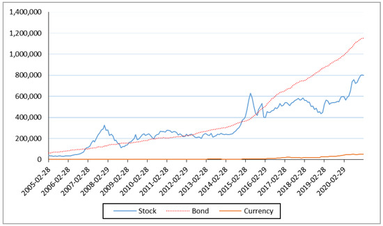
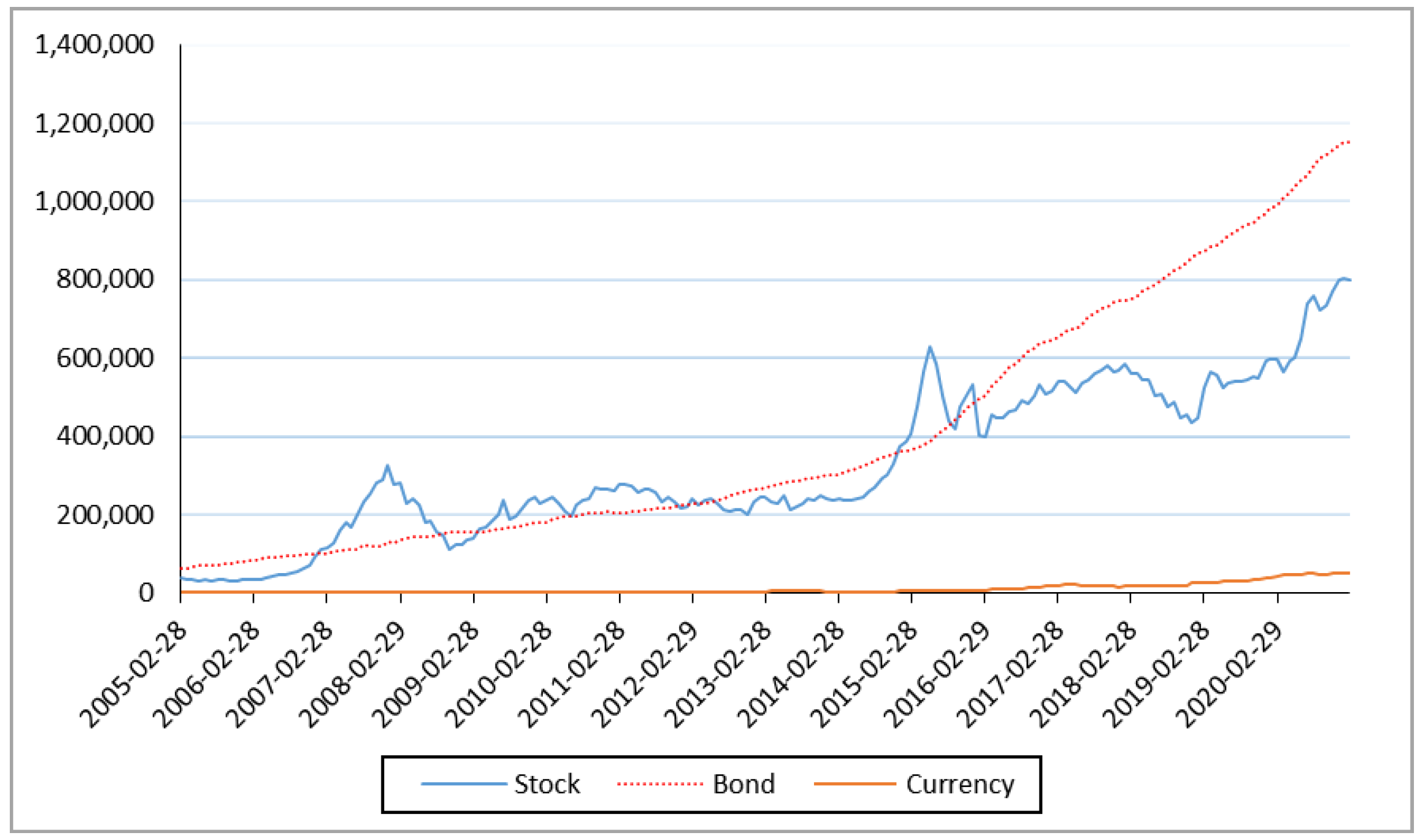
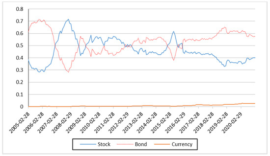
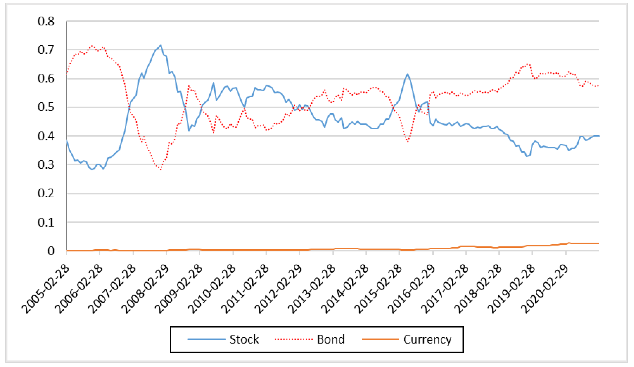
The final equilibrium returns were obtained through the market values of the three asset classes as follows, see Figure 3 and Figure 4.

Figure 3. Market value changes of the three types of assets.

Figure 4. Equilibrium return changes of the three types of assets.

We selected the annualized rate of return, annualized volatility, and Sharpe ratio as the indexes for comparative analysis.

The actual data from February 2016 to February 2021 were used as the backtesting interval for asset allocation. The annualized rate of return of the final portfolio decision was derived based on different risk aversion coefficients for pension asset allocation. The annualized volatility and Sharpe ratio are listed in Table 4.

Table 4. The annualized rate of return and annualized volatility of the proposed model and the models for comparison.

Risk Aversion Coefficient	Models	Annualized Rate of Return (%)	Annualized Volatility (%)	Sharpe Ratio
1	Traditional BL model	4.77	5.05	0.69
	TVC-BL	4.78	4.45	0.78
1.5	Traditional BL model	4.76	4.56	0.76
	TVC-BL	4.70	4.03	0.84
2.5	Traditional BL model	4.68	4.32	0.78
	TVC-BL	4.66	3.83	0.88

According to Table 4, the TVC-BL pension asset allocation model with time-varying covariance as the risk estimate outperforms the traditional BL pension asset allocation model in terms of asset allocation effectiveness. In terms of the annualized rate of return, the difference between the two models is not significant, but in terms of annualized volatility, the TVC-BL model achieves a significantly lower value than the traditional BL model. In terms of the Sharpe ratio, the TVC-BL model achieves a significantly higher value than that of the traditional BL model. The results indicate that the proposed TVC-BL pension asset allocation model outperforms the traditional BL model. When the risk aversion coefficient is 1, 1.5, and 2.5, the Sharp ratio of pension asset allocation through the TVC-BL pension asset allocation model is 13.0%, 10.5%, and 12.8% higher than that of the traditional BL model.

4.5. Discussion

In this subsection, we further analyze the effectiveness of the proposed TVC-BL model.

Ma et.al. proposed a mean-variance with forecasting (MVF) model for portfolio optimization, and the mean-variance with random forests (RF-MV) model outperformed the benchmark models [53].

We extended the RF-MV model to the RF-BL model by replacing the MV method with the BL method. Furthermore, we added TVC into the RF-MV model and obtained the RF-BL-TVC model. The annualized volatility and Sharpe ratio of the RF-BL model and RF-BL-TVC model are listed in Table 5.

Table 5. The annualized rate of return and annualized volatility of RF-BL model and RF-BL-TVC model.

Risk Aversion Coefficient	Model	Annualized Rate of Return (%)	Annualized Volatility (%)	Sharpe Ratio
1	RF-BL	4.90	5.07	0.71
	RF-BL-TVC	4.91	4.52	0.80
1.5	RF-BL	4.82	4.62	0.76
	RF-BL-TVC	4.83	4.13	0.85
2.5	RF-BL	4.75	4.42	0.78
	RF-BL-TVC	4.78	3.91	0.89

According to Table 5, the RF-BL-TVC model with time-varying covariance as the risk estimate outperforms the RF-BL model in terms of asset allocation effectiveness. In terms of the Sharpe ratio, the RF-BL-TVC model achieves a significantly higher value than the RF-BL model. The results indicate that the RF-BL-TVC model outperforms the RF-BL model. When the risk aversion coefficient is 1, 1.5, and 2.5, the Sharp ratio of pension asset allocation through the RF-BL-TVC pension asset allocation model is 12.7%, 11.8%, and 14.1% higher than that of the RF-BL model.

Based on the analysis of the results in Table 4 and Table 5, we found that the models with TVC outperform consistently for optimal pension asset allocation.

5. Conclusions

Due to the long term of pension asset allocation decisions and the insufficiency of asset history data, calculating the long-term covariance matrix directly from historical data faces the problem of insufficient sample data, leading to the failure of covariance matrix estimations. The commonly used solution is directly modeling the monthly ROA data to obtain the monthly covariance matrices and accumulating them to produce the covariance matrices of other terms. However, the covariance matrix of asset returns tends to exhibit dynamic changes due to the relatively strong autocorrelation of major asset class returns. Therefore, the long-term covariance matrix obtained directly by accumulating monthly covariance matrices tends to be somewhat problematic.

In this paper, we first modeled ROA and the covariance of ROA by VARMA and GARCH and studied the effective conversion method from a short-term covariance matrix to a long-term covariance matrix. On that basis, a TVC-BL pension asset allocation model with time-varying covariance as the risk estimate was constructed and applied to pension asset allocation to produce the asset allocation decisions. A performance comparison revealed that the proposed TVC-BL pension asset allocation model outperformed the traditional BL pension asset allocation model in terms of asset allocation effectiveness after considering the time-varying covariance.

References

- Yan, Y.P.; Huang, M.X.; Zheng, Y.R. Study on the Change and Trend of Age Structure of Chinese Population. Dongyue Trib. 2021, 1, 148–163. [Google Scholar]
- Hui, H.; Sun, H. A Research on the Contradiction between Private and Public Pension Industries in China—Take Chongqing as an Example. J. Serv. Sci. Manag. 2021, 14, 151–159. [Google Scholar] [CrossRef]
- Brennan, M.J.; Schwartz, E.S.; Lagnado, R. Strategic Asset Allocation. J. Econ. Dyn. Control. 1997, 21, 1377–1403. [Google Scholar] [CrossRef] [Scilit]
- Campbell, J.Y.; Viceira, L.M. Appendix for "Strategic Asset Allocation: Portfolio Choice for Long-Term Investors"; Oxford University Press: Oxford, UK, 2002. [Google Scholar]
- Rey, D. Current Research Topics-Stock Market Predictability: Is it There? Financ. Mark. Portf. Manag. 2003, 17, 379–387. [Google Scholar]
- Farrell, J.L.; Reinhart, W.J. Portfolio Management: Theory and Application, 2nd ed.; Mc Graw-Hill Companies. Inc.: New York, NY, USA, 1997. [Google Scholar]
- Chowdhury, S.S.H.; Rahman, M.A.; Sadique, M.S. Stock return autocorrelation, day of the week and volatility: An empirical investigation on the Saudi Arabian stock market. Rev. Account. Financ. 2017, 16, 218–238. [Google Scholar] [CrossRef] [Scilit]
- Sim, N. Estimating the Correlation of Asset Returns: A Quantile Dependence Perspective; Handbook of Financil Economerics and Statistics; Springer: New York, NY, USA, 2015; pp. 1829–1855. [Google Scholar]
- Stoll, H.R.; Whaley, R.E. The Dynamics of Stock Index and Stock Index Futures Returns. J. Financ. Quant. Anal. 1990, 25, 441–468. [Google Scholar] [CrossRef] [Scilit]
- Ding, Z.; Engle, R.F. Large Scale Conditional Covariance Matrix Modeling, Estimation and Testing. Acad. Econ. Pap. 2001, 2. Available online: http://hdl.handle.net/2451/26888 (accessed on 1 January 2023).
- Campbell, J.Y.; Viceira, L.M. Strategic Asset Allocation; Oxford University Press: Oxford, UK, 2002. [Google Scholar]
- Markowitz, H.M. Portfolio Selection. J. Financ. 1952, 7, 77–91. [Google Scholar]
- Markowitz, H.M. Portfolio Selection: Efficient Diversification of Investment; Basil Blackwell: New York, NY, USA, 1959. [Google Scholar]
- Tobin, J. Liquidity Preference as Behavior towards Risk. Rev. Econ. Studies. 1958, 25, 68–85. [Google Scholar] [CrossRef] [Scilit]
- Sharpe, W.F. Capital Asset Prices: A Theory of Market Equilibrium Under Conditions of Risk. J. Financ. 1964, 19, 425–442. [Google Scholar]
- Lintner, J. The Valuation of Risk Assets and The Selection of Risky Investments in Stock Portfolios and Capital Budgets. Rev. Econ. Stat. 1965, 47, 13–37. [Google Scholar] [CrossRef] [Scilit]
- Mossin, J. Equilibrium in a Capital Asset Market. Econometrica 1966, 34, 768–783. [Google Scholar] [CrossRef] [Scilit]
- Black, F.; Litterman, R. Global portfolio optimization. Financ. Anal. J. 1992, 48, 28–42. [Google Scholar] [CrossRef] [Scilit]
- Black, F.; Litterman, R. Asset allocation: Combining investor views with market quilibrium. J. Fixed Lncome. 1991, 1, 7–18. [Google Scholar] [CrossRef] [Scilit]
- Dutta, J.; Kapur, S.; Orszag, J.M. A portfolio approach to the optimal funding of pensions. Econ. Lett. 2000, 69, 201–206. [Google Scholar] [CrossRef] [Scilit]
- Parra, M.A.; Terol, A.B.; Uria, M.R. A fuzzy goal programming approach to portfolio selection. Eur. J. Oper. Res. 2001, 133, 287–297. [Google Scholar] [CrossRef] [Scilit]
- Booth, P.; Yakoubov, Y. Investment policy for defined-contribution pension scheme members close to retirement: An analysis of the “lifestyle” concept. North Am. Actuar. J. 2000, 4, 1–19. [Google Scholar] [CrossRef] [Scilit]
- Blake, D.; Cairns, A.J.; Dowd, K. Pensionmetrics: Stochastic pension plan design and value-at-risk during the accumulation phase. Insur. Math. Econ. 2001, 29, 187–215. [Google Scholar] [CrossRef] [Scilit]
- Haberman, S.; Vigna, E. Optimal investment strategies and risk measures in defined contribution pension schemes. Insur. Math. Econ. 2002, 31, 35–69. [Google Scholar] [CrossRef] [Scilit]
- Sherris, M. Portfolio Selection Models for Life Insurance and Pension Funds. 3rd AFIR Int. Colloq. 2022, 119, 87–105. [Google Scholar]
- Defau, L.; Moor, L.D. The investment behaviour of pension funds in alternative assets: Interest rates and portfolio diversification. Int. J. Financ. Econ. 2021, 26, 1424–1434. [Google Scholar] [CrossRef] [Scilit]
- Lin, C.W.; Zeng, L.; Wu, H.L. Multi-Period Portfolio Optimization in a Defined Contribution Pension Plan during the Decumulation Phase. J. Ind. Manag. Optim. 2019, 15, 401–427. [Google Scholar] [CrossRef] [Scilit]
- Luchko, M.; Lew, G.; Ruska, R.; Vovk, I. Modelling the optimal size of investment portfolio in a non-state pension fund. Cent. Sociol. Res. NGO 2019, 12, 239–253. [Google Scholar] [CrossRef] [Scilit]
- Tiro, K.; Basimanebotlhe, O.; Offen, E.R. Stochastic Analysis on Optimal Portfolio Selection for DC Pension Plan with Stochastic Interest and Inflation Rate. J. Math. Financ. 2021, 11, 579–596. [Google Scholar] [CrossRef]
- Bevan; Winkelmann, K. Using the Black-Litterman Globa1 Asset Allocation Model: Three Years of Practica1 Experience; Fixed Income Research; Goldman, Sachs& Company: New York, NY, USA, 1998. [Google Scholar]
- Qian, E.; Gorman, S. Conditional Distribution in Portfolio Theory. Financ. Anal. J. 2001, 57, 44–51. [Google Scholar] [CrossRef] [Scilit]
- Beach, S.L.; Orlov, A.G. An Application of the Black-Litterman Model with EGARCH-M-Derived views for International Portfolio Management. Financ. Mark. Portf. Manag. 2006, 21, 147–166. [Google Scholar] [CrossRef] [Scilit]
- Ta, B.Q.; Vuong, T. The Black-Litterman model for portfolio optimization on Vietnam stock market. Int. J. Uncertain. Fuzziness Knowl.-Based Syst 2020, 28 (Suppl. 1), 99–111. [Google Scholar] [CrossRef] [Scilit]
- Lin, W.H.; Teng, H.W.; Yang, C.C. A Heteroskedastic Black–Litterman Portfolio Optimization Model with Views Derived from a Predictive Regression. Handb. Financ. Econom. Math. Stat. Mach. Learn. 2020, 563–581. [Google Scholar] [CrossRef] [Scilit]
- Teplova, T.; Evgeniia, M.; Munir, Q.; Pivnitskaya, N. Black-Litterman model with copula-based views in mean-CVaR portfolio optimization framework with weight constraints. Econ. Change Restruct. 2022, 56, 515–535. [Google Scholar] [CrossRef] [Scilit]
- Martellini, L.; Ziemann, V. Extending Black-Littermman Analysis Beyond the Mean-Variance Framework. J. Portf. Manag. 2007, 33, 33–44. [Google Scholar] [CrossRef] [Scilit]
- Cheung, W. The Augmented Black-Litterman Model: A ranking-free approach to factou-based portfolio construction and beyond. Quant. Financ. 2013, 13, 301–316. [Google Scholar] [CrossRef] [Scilit]
- O'Toole, R. The Black–Litterman model: A Risk Budgeting Perspective. J. Asset Manag. 2013, 14, 2–13. [Google Scholar] [CrossRef] [Scilit]
- Miťková, V.; Mlynarovič, V. A performance and risk analysis on the Slovak private pension funds market. J. Econ. 2007, 3, 232–249. [Google Scholar]
- Park, Y.K.; Kim, H.; Joo, H. Alternative Investment Portfolio Analysis for the Korean National Pension Fund. Asian Rev. Financ. Res. 2015, 28, 235–267. [Google Scholar]
- Platanakis, E.; Sutcliffe, C. Asset–liability modelling and pension schemes: The application of robust optimization to USS. Eur. J. Financ. 2017, 23, 324–352. [Google Scholar] [CrossRef] [Scilit]
- Buriticá-Mejía, J.A. Modelo Black-Litterman con Support Vector Regression: Una alternativa para los fondos de pensiones obligatorios colombianos (Black-Litterman Model with Support Vector Regression: An Alternative for Colombian Pension Funds). ODEON 2020, 18, 205–257. [Google Scholar] [CrossRef] [Scilit]
- Stoilov, T.; Stoilova, K.; Vladimirov, M. Application of modified Black-Litterman model for active portfolio management. Expert Syst. Appl. 2021, 186, 115719. [Google Scholar] [CrossRef] [Scilit]
- Simos, T.E.; Mourtas, S.D.; Katsikis, V.N. Time-varying Black–Litterman portfolio optimization using a bio-inspired approach and neuronets. Appl. Soft Comput. 2021, 112, 107767. [Google Scholar] [CrossRef] [Scilit]
- Barua, R.; Sharma, A.K. Dynamic Black Litterman portfolios with views derived via CNN-BiLSTM predictions. Financ. Res. Lett. 2022, 49, 103111. [Google Scholar] [CrossRef] [Scilit]
- Klein, R.W.; Bawa, V.S. The effect of estimation risk on optimal portfolio choice. J. Financ. Econ. 1976, 3, 215–231. [Google Scholar] [CrossRef] [Scilit]
- Ankrim, E.; Fox, S.; Hensel, C. Commodities in Asset Allocation: A Real-Asset Alternative to Real Estate. Financ. Anal. J. 1993, 49, 20–29. [Google Scholar] [CrossRef] [Scilit]
- Ding, Z.; Martin, R.D. The Fundamental Law of Active Management: Redux. J. Empir. Financ. 2017, 43, 91–114. [Google Scholar] [CrossRef] [Scilit]
- Cong, F.; Oosterlee, C.W. Multi-period mean-variance portfolio optimization based on monte-carlo simulation. J. Econ. Dyn. Control. 2016, 64, 23–38. [Google Scholar] [CrossRef] [Scilit]
- De la Torre-Torres, O.V.; Venegas-Martínez, F.; Martínez-Torre-Enciso, M.I. Enhancing portfolio performance and VIX futures trading timing with markov-switching GARCH models. Mathematics 2021, 9, 185. [Google Scholar] [CrossRef] [Scilit]
- Escobar-Anel, M.; Gollart, M.; Zagst, R. Closed-form portfolio optimization under GARCH models. Oper. Res. Perspect. 2022, 9, 100216. [Google Scholar] [CrossRef] [Scilit]
- Dufour, J.M.; Pelletier, D. Practical methods for modeling weak VARMA processes: Identification, estimation and specification with a macroeconomic application. J. Bus. Econ. Stat. 2021, 40, 1140–1152. [Google Scholar] [CrossRef] [Scilit]
- Yilin, M.; Han, R.; Wang, W. Portfolio optimization with return prediction using deep learning and machine learning. Expert Syst. Appl. 2021, 165, 113973. [Google Scholar]
Disclaimer/Publisher’s Note: The statements, opinions and data contained in all publications are solely those of the individual author(s) and contributor(s) and not of MDPI and/or the editor(s). MDPI and/or the editor(s) disclaim responsibility for any injury to people or property resulting from any ideas, methods, instructions or products referred to in the content. |
© 2023 by the authors. Licensee MDPI, Basel, Switzerland. This article is an open access article distributed under the terms and conditions of the Creative Commons Attribution (CC BY) license (https://creativecommons.org/licenses/by/4.0/).