On Consistency of the Nearest Neighbor Estimator of the Density Function for m-AANA Samples

Abstract

In this paper, by establishing a Bernstein inequality for m-asymptotically almost negatively associated random variables, some results on consistency for the nearest neighbor estimator of the density function are further established. The results generalize some existing ones in the literature. Some numerical simulations are also provided to support the results.

1. Introduction

Nearest neighbor estimators can be used for many flexible questions and data types. Let X be a random variable whose density function $f\left(x\right)$ is unknown and needs to be estimated. Let $X_1,X_2,\cdots ,X_n$ be the sample drawn from population X. To estimate $f\left(x\right)$, Loftsgarden and Quesenberry [1] raised the nearest neighbour estimator $f_n\left(x\right)$ as follows:

$$\begin{array}{c}\hfill f_n\left(x\right)=\frac{k_n}{2n{a}_n\left(x\right)},\end{array}$$

(1)

where $1\le k_n\le n$ and

$$a_n\left(x\right)=min\{\alpha :\mathrm{the}\mathrm{number}\mathrm{of}{X}_i\in [x-\alpha ,x+\alpha ]\mathrm{is}\mathrm{no}\mathrm{less}\mathrm{than}{k}_n\}.$$

Since Loftsgarden and Quesenberry [1] put forward the method of estimating the density function, many scholars showed their interest in this field. For some recent examples, Liu and Wu [2] established the Bernstein inequality to deal with the consistency results under negatively dependent samples; Lu et al. [3] investigated some results on consistency and convergence rate for this estimator based on $\phi$-mixing samples; Liu and Zhang [4] established the consistency and asymptotic normality of the estimator based on $\alpha$-mixing samples; Yang [5] established various results on the consistency of the estimator based on negatively associated (NA, in short) samples; Wang and Hu [6] obtained the corresponding results for widely orthant dependent (WOD, in short) samples, which extend and improve those of Yang [5] for NA samples and further proved the rates of strong consistency and uniformly strong consistency; Lan and Wu [7] investigated the rate of uniform strong consistency for the estimator under extended negatively dependent (END, in short) samples; and Wang and Wu [8] extended and improved the results of Lan and Wu [7] from END samles to m-extended negatively dependent (m-END, in short) samples and obtained the same rates as that of END samples.

This paper will further study this topic and extend those aforementioned results to a more general setting. Now, we are at a position to recall some concepts of dependent random variables, of which the first one is that of asymptotically almost negatively associated (AANA, in short) random variables, which was first raised by Chandra and Ghosal [9] as follows.

Definition 1.

We call a sequence $\{Z_n,n\ge 1\}$ of random variables to be AANA if there is a nonnegative sequence satisfying ${lim}_{n\to \infty }q\left(n\right)=0$ such that for all $n,l\ge 1$ and for all coordinatewise nondecreasing functions $f_1$ and $f_2$,

$$Cov(f_1\left(Z_n\right),f_2(Z_{n+1},Z_{n+2},\cdots ,Z_{n+l}))\le q\left(n\right){\left[Var\left(f_1\left(Z_n\right)\right)Var\left(f_2(Z_{n+1},Z_{n+2},\cdots ,Z_{n+l})\right)\right]}^{1/2}$$

whenever the variances above exist.

Since the concept of AANA random variables was put forward by Chandra and Ghosal [9], plenty of results have been established concerning this dependence structure. For instance, Kim and Ko [10] developed the Hajeck–Renyi inequality for these dependent random variables; Yuan and An [11] established some moment inequalities for maximum sums; Chandra and Ghosal [12] as well as Shen and Wu [13] proved the strong law of large numbers for weighted sums; Yuan and An [14] investigated the laws of large numbers for this dependent random variables satisfying the Cesàro alpha-integrability condition; and Wu and Wang [15] studied some results on the nearest neighbor estimator of the density function under AANA samples.

As an extension of AANA random variables, the concept of m-AANA random variables was raised by Nam et al. [16] as follows.

Definition 2.

Let m be a positive integer. We say that a sequence $\{Z_n,n\ge 1\}$ of random variables is m-AANA if there exists a nonnegative sequence $q\left(n\right)\to 0$ as $n\to \infty$ such that for all $n,l\ge m$ and for all coordinatewise nondecreasing functions $f_1$ and $f_2$,

$$Cov(f_1\left(Z_n\right),f_2(Z_{n+m},\cdots ,Z_{n+l}))\le q\left(n\right){\left[Var\left(f_1\left(Z_n\right)\right)Var\left(f_2(Z_{n+m},\cdots ,Z_{n+l})\right)\right]}^{1/2}$$

whenever the variances exist.

It is known that many multivariate distributions satisfy the NA property. The concept of AANA random variables will degenerate to that of NA random variables by taking $q\left(n\right)=0$. It is easy to see that the m-AANA sequence is equivalent to AANA with $m=1$. Therefore, the structure of m-AANA random variables includes AANA random variables, m-NA random variables, NA random variables, moving average processes, and independent random variables as special cases, and thus it is a more plausible assumption in realistic applications. Now, we present an example of m-AANA random variables that are not necessarily AANA.

Example 1.

Let $\{Y_n,n\ge 1\}$ be independent and identically distributed $N(0,1)$ random variables and define $X_n={(1+a_n^2)}^{-1/2}(Y_n+a_n{Y}_{n+1})$, where $a_n>0$ and $a_n\to 0$. It follows from Chandra and Ghosal [9] that $\{X_n,n\ge 1\}$ is a sequence of AANA random variables that is not NA. Now, we define for each $n\ge 1$ that $Z_{m(n-1)+1}=\cdots =Z_{mn}=X_n$ with $m\ge 2$. Then, it is easy to check that the sequence $\{Z_n,n\ge 1\}$ is m-AANA. However, it is not AANA since the condition ${lim}_{n\to \infty }q\left(n\right)=0$ is not satisfied if we take $l=1$, for example.

In this paper, motivated by the literature above, we first establish a Bernstein inequality for m-asymptotically almost negatively associated (m-AANA, in short) random variables, which is of interest itself. By using this inequality, we further investigate some results on the consistency of the nearest neighbor estimator under m-AANA samples. These results are generalizations of the corresponding ones of Wu and Wang [15] from AANA samples to m-AANA samples.

The layout of this paper is as follows. Some preliminary lemmas are stated in Section 2. Section 3 includes the main results, while the numerical simulations are given in Section 4 to support the theoretical results. The proofs of our main results are postponed in Section 5. The paper is concluded in Section 6. Throughout this paper, $\lfloor x\rfloor$ stands for the integer part of x. Let $logx=max\{1,lnx\}$. Indicator function $I\left(A\right)=1$ if the set A occurs or $I\left(A\right)=0$ otherwise. $C\left(f\right)=\{x:f\mathrm{is}\mathrm{continuous}\mathrm{at}x\}$. C and $c_0$ stand for positive constants whose values are not necessarily the same in each appearance. All limits are taken as $n\to \infty$ unless specified otherwise.

2. Preliminary Lemmas

To prove the main results, we first provide several important lemmas in this section.

Lemma 1

(cf. [14]). Suppose that $\{X_n,n\ge 1\}$ is a sequence of AANA random variables with mixing coefficients $\left\{q\right(n),n\ge 1\}$. If $f_n(·),n\ge 1$ are all nondecreasing or all nonincreasing, then $\{f_n\left(X_n\right),n\ge 1\}$ is still a sequence of AANA random variables with the same mixing coefficients.

A combination of Lemma 1 and Definition 2 yields the following lemma, which is obvious, and thus the proof is omitted.

Lemma 2.

Suppose that $\{X_n,n\ge 1\}$ is a sequence of m-AANA random variables with mixing coefficients $\left\{q\right(n),n\ge 1\}$. If $f_n(·),n\ge 1$ are all nondecreasing or all nonincreasing; then, $\{f_n\left(X_n\right),n\ge 1\}$ is still a sequence of m-AANA random variables with the same mixing coefficients.

Lemma 3

(cf. [15]). Let $\{X_n,n\ge 1\}$ be a sequence of AANA random variables with zero means and mixing coefficients $\left\{q\right(n),n\ge 1\}$. Assume that $|X_n|$ is bounded by a positive number b for each $n\ge 1$. Then, a positive constant C exists such that for all $n\ge 1$ and $\epsilon >0$,

$$\begin{array}{c}\hfill P\left(\left|\sum _{i=1}^n{X}_i\right|\ge \epsilon \right)\le C\left[\sum _{k=1}^{n-1}q\left(k\right)+1\right]·exp\left\{-\frac{{\epsilon }^2}{2{\sum }_{i=1}^{n}E{X}_i^2+\frac{2}{3}b\epsilon }\right\}.\end{array}$$

(2)

By virtue of Lemma 3, we can further prove the Bernstein inequality for m-AANA random variables. The lemma will play a significant role in the proof of the main results.

Lemma 4.

Let $\{X_n,n\ge 1\}$ be a sequence of m-AANA random variables with zero means and mixing coefficients $\left\{q\right(n),n\ge 1\}$. Assume that $|X_n|$ is bounded by a positive number b for each $n\ge 1$. Then, a positive constant C exists such that for all $n\ge 1$ and $\epsilon >0$,

$$\begin{array}{c}\hfill P\left(\left|\sum _{i=1}^n{X}_i\right|\ge \epsilon \right)\le Cm\left[\sum _{k=1}^{n-1}q\left(k\right)+1\right]·exp\left\{-\frac{\frac{{\epsilon }^2}{m^2}}{2{\sum }_{i=1}^n{X}_i+\frac{2}{3m}b\epsilon }\right\}.\end{array}$$

Proof. 

For all sufficiently large n, positive integers $j\ge 0$ and $1\le l\le m$ always exist satisfying $n=mj+l$. Without a loss of generality, we may define that $X_i=0$ for all $n<i\le m(j+1)$. Thus, ${\sum }_{i=1}^n{X}_i$ can be decomposed as

$$\begin{array}{c}\hfill \sum _{i=1}^n{X}_i=\sum _{l=1}^m\sum _{i=0}^j{X}_{mi+l}\end{array}$$

where $\{X_{mi+l},0\le i\le j\}$ are AANA for each given $l=1,2,\cdots ,m$. Thus, we can obtain from Lemma 3 that

$$\begin{array}{ccc}\hfill P\left(\left|S_n\right|\ge \epsilon \right)& =& P\left(\left|\sum _{l=1}^m\sum _{i=0}^j{X}_{mi+l}\right|\ge \epsilon \right)\hfill \\ & \le & P\left(\bigcup _{l=1}^m\left|\sum _{i=0}^j{X}_{mi+l}\right|\ge \frac{\epsilon }{m}\right)\hfill \\ & \le & \sum _{l=1}^{m}P\left(\left|\sum _{i=0}^j{X}_{mi+l}\right|\ge \frac{\epsilon }{m}\right)\hfill \\ & \le & C\sum _{l=1}^m\left[\sum _{k=1}^{j-1}q\left(k\right)+1\right]·exp\left\{-\frac{\frac{{\epsilon }^2}{m^2}}{2\times {\sum }_{i=0}^{j}E{\left(X_{mi+l}\right)}^2+\frac{2}{3m}b\epsilon }\right\}\hfill \\ & \le & Cm\left[\sum _{k=1}^{n-1}q\left(k\right)+1\right]·exp\left\{-\frac{\frac{{\epsilon }^2}{m^2}}{2B_n^2+\frac{2}{3m}b\epsilon }\right\}\hfill \end{array}$$

This completes the proof of the lemma. □

Lemma 5

(cf. [5]). Let $Z_1,Z_2,\cdots ,Z_n$ follow a common distribution $F\left(z\right)$, which is continuous. For $n\ge 3$, assume that $z_{ni}$ satisfies $F\left(z_{ni}\right)=i/n$ for each $1\le i\le n-1$. Then,

$$\begin{array}{c}\hfill \underset{-\infty <z<\infty }{sup}|F_n\left(z\right)-F\left(z\right)|\le \underset{1\le i\le n-1}{max}|F_n\left(z_{ni}\right)-F\left(z_{ni}\right)|+2/n,\end{array}$$

where $F_n\left(z\right)=n^{-1}{\sum }_{j=1}^{n}I(Z_j<z)$ is the empirical distribution function.

Lemma 6.

Let $\{Z_n,n\ge 1\}$ be a sequence of m-AANA random variables, with $F\left(z\right)$ and $f\left(z\right)$ being the distribution function and density function, respectively. Let $\{{\kappa }_n,n\ge 1\}$ be a sequence of positive numbers satisfying ${\kappa }_n\to 0$ such that ${lim\; inf}_{n\to \infty }n{\kappa }_n^2/logn\ge c_0>0$. Then, for any $D_0>0$ large enough,

$$\begin{array}{c}\hfill \sum _{n=1}^{\infty }P\left(\underset{z}{sup}|F_n\left(z\right)-F\left(z\right)|>D_0{\kappa }_n\right)<\infty .\end{array}$$

In particular,

$$\begin{array}{c}\hfill \sum _{n=1}^{\infty }P\left(\underset{z}{sup}|F_n\left(z\right)-F\left(z\right)|>D_0{(logn/n)}^{1/2}\right)<\infty .\end{array}$$

Proof. 

Observing that $n{\kappa }_n\to \infty$, we have that $2/n<D_0{\kappa }_n/2$ for all sufficiently large n and any positive constant $D_0$, the value of which will be specified later. It follows from Lemma 5 that

$$\begin{array}{ccc}\hfill P\left(\underset{x}{sup}|F_n\left(x\right)-F\left(x\right)|>D_0{\kappa }_n\right)& \le & P\left(\underset{1\le i\le n-1}{max}|F_n\left(x_{ni}\right)-F\left(x_{ni}\right)|>D_0{\kappa }_n/2\right)\hfill \\ & \le & \sum _{i=1}^{n-1}P\left(\right|F_n\left(z_{ni}\right)-F\left(z_{ni}\right)|>D_0{\kappa }_n/2).\hfill \end{array}$$

(3)

Let $Z_j\left(z_{ni}\right)=I(Z_j<z_{ni})-EI(Z_j<z_{ni})$. By Lemma 2, we know that $\{Z_j\left(z_{ni}\right),j\ge 1\}$ is still a sequence of m-AANA random variables with $E{Z}_j\left(z_{ni}\right)=0$, $|Z_j\left(z_{ni}\right)|\le 1$ and $E{\left(Z_j\left(z_{ni}\right)\right)}^2\le 1$. Thus, by Lemma 4 we have that for all n adequately large,

$$\begin{array}{ccc}\hfill P\left(\right|F_n\left(z_{ni}\right)-F\left(z_{ni}\right)|>D_0{\kappa }_n/2)& =& P\left(\left|\sum _{j=1}^n{Z}_j\left(z_{ni}\right)\right|>D_{0}n{\kappa }_n/2\right)\hfill \\ & \le & C_m\left[\sum _{k=1}^{n-1}q\left(k\right)+1\right]·exp\left\{\frac{-\frac{D_0^2{n}^2{\kappa }_n^2}{m^2}}{8B_n^2+\frac{4}{3m}{D}_{0}n{\kappa }_n}\right\}\hfill \\ & \le & Cnexp\left\{-\frac{D_0^2}{9m^2}n{\kappa }_n^2\right\}\hfill \\ & \le & Cnexp\left\{-\frac{c_0{D}_0^2}{18m^2}logn\right\}\hfill \\ & \le & C{n}^{1-\frac{c_0{D}_0^2}{18m^2}}.\hfill \end{array}$$

(4)

Taking $D_0$ sufficiently large such that $1-\frac{c_0{D}_0^2}{18m^2}<-2$, by (3) and (4) we have

$$\begin{array}{ccc}\hfill \sum _{n=1}^{\infty }P\left(\underset{z}{sup}|F_n\left(z\right)-F\left(z\right)|>D_0{\kappa }_n\right)& \le & C\sum _{n=1}^{\infty }\sum _{j=1}^{n-1}{n}^{1-\frac{c_0{D}_0^2}{18m^2}}<\infty .\hfill \end{array}$$

This completes the proof of the lemma. □

3. Main Results

Now, we state our results one by one as follows. Denote ${\chi }_n={\sum }_{k=1}^{n-1}q\left(k\right)+1$. The first one concerns the weak consistency of the nearest neighbor density estimator.

Theorem 1.

Suppose that $\{X_n,n\ge 1\}$ is a sequence of m-AANA samples and $k_n/n\to 0$, $k_n^2/n\to \infty$. If

$$\begin{array}{c}\hfill \underset{n\to \infty }{lim}{\chi }_n·exp\left\{-\frac{\gamma k_n^2}{n}\right\}=0\end{array}$$

(5)

for all $\gamma >0$, then for all $x\in c\left(f\right)$,

$$\begin{array}{c}\hfill f_n\left(x\right)\stackrel{P}{\to }f\left(x\right).\end{array}$$

Remark 1.

We point out that (5) is easy to verify. For example, if ${\sum }_{n=1}^{\infty }q\left(n\right)<\infty$, which is frequently adopted in the literature, we have ${\chi }_n\le 1+{\sum }_{n=1}^{\infty }q\left(n\right)<\infty$ and thus (5) follows. Moreover, if $k_n^2/(nlogn)\to \infty$, (5) also holds without any restriction on the mixing coefficients. We give it in the following corollary.

Corollary 1.

Let $\{X_n,n\ge 1\}$ be a sequence of m-AANA samples and $k_n/n\to 0$, $k_n^2/(nlogn)\to \infty$. Then, for all $x\in c\left(f\right)$,

$$\begin{array}{c}\hfill f_n\left(x\right)\stackrel{P}{\to }f\left(x\right).\end{array}$$

Under some slightly stronger conditions, one can obtain the following results on complete consistency.

Theorem 2.

Let $\{X_n,n\ge 1\}$ be a sequence of m-AANA samples and $k_n/n\to 0$, $k_n^2/n\to \infty$. If

$$\begin{array}{c}\hfill \sum _{n=1}^{\infty }{\chi }_{n}exp\left\{-\frac{\gamma k_n^2}{n}\right\}<\infty \end{array}$$

(6)

for all $\gamma >0$, then for all $x\in c\left(f\right)$,

$$\begin{array}{c}\hfill \sum _{n=1}^{\infty }P\left(\right|f_n\left(x\right)-f\left(x\right)|>\epsilon )<\infty \end{array}$$

for all $\epsilon >0$, and hence

$$\begin{array}{c}\hfill f_n\left(x\right)\to f\left(x\right)a.s.\end{array}$$

By some analogous argument to that of Corollary 1, the following conclusion can also be obtained.

Corollary 2.

Let $\{X_n,n\ge 1\}$ be a sequence of m-AANA samples and $k_n/n\to 0$, $k_n^2/(nlogn)\to \infty$. Then, for all $x\in c\left(f\right)$,

$$\begin{array}{c}\hfill \sum _{n=1}^{\infty }P\left(\right|f_n\left(x\right)-f\left(x\right)|>\epsilon )<\infty \end{array}$$

for all $\epsilon >0$, and hence

$$\begin{array}{c}\hfill f_n\left(x\right)\to f\left(x\right)a.s.\end{array}$$

Moreover, we can further obtain the rate of complete consistency for the nearest neighbor density estimator as follows.

Theorem 3.

Let $\{X_n,n\ge 1\}$ be a sequence of m-AANA samples and $f\left(x\right)$ satisfy the local Lipschitz condition at x and $f\left(x\right)>0$. If $k_n=O\left(n^{3/4}{log}^{1/4}n\right)$ and ${\tau }_n=:\sqrt{nlogn}/k_n\to 0$; then, for all sufficiently large $D>0$,

$$\begin{array}{c}\hfill \sum _{n=1}^{\infty }P\left(\right|f_n\left(x\right)-f\left(x\right)|>D{\tau }_n)<\infty ,\end{array}$$

and hence

$$\begin{array}{c}\hfill |f_n\left(x\right)-f\left(x\right)|\le D{\tau }_{n}a.s.\end{array}$$

By choosing $k_n=\lfloor n^{3/4}{log}^{1/4}n\rfloor$ in Theorem 3, the following result follows immediately.

Corollary 3.

Let $\{X_n,n\ge 1\}$ be a sequence of m-AANA samples, and let $f\left(x\right)$ satisfy the local Lipschitz condition at x and $f\left(x\right)>0$. If $k_n=\lfloor n^{3/4}{log}^{1/4}n\rfloor$, then for all sufficiently large $D>0$,

$$\begin{array}{c}\hfill \sum _{n=1}^{\infty }P\left(|f_n\left(x\right)-f\left(x\right)|>D{n}^{-1/4}{log}^{1/4}n\right)<\infty ,\end{array}$$

and hence

$$\begin{array}{c}\hfill |f_n\left(x\right)-f\left(x\right)|\le D{n}^{-1/4}{log}^{1/4}na.s.\end{array}$$

At last, we also obtain some achievements concerning uniform consistency and the corresponding convergence rate for the estimator as follows.

Theorem 4.

Let $\{X_n,n\ge 1\}$ be a sequence of m-AANA samples and $f\left(x\right)$ be uniformly continuous. If $k_n/n\to 0$, $k_n^2/(nlogn)\to \infty$, then for all $\epsilon >0$,

$$\begin{array}{c}\hfill \sum _{n=1}^{\infty }P\left(\underset{x}{sup}|f_n\left(x\right)-f\left(x\right)|>\epsilon \right)<\infty ,\end{array}$$

and hence

$$\begin{array}{c}\hfill \underset{x}{sup}|f_n\left(x\right)-f\left(x\right)|\to 0a.s.\end{array}$$

Theorem 5.

Let $\{X_n,n\ge 1\}$ be a sequence of m-AANA samples and let $f\left(x\right)$ satisfy the Lipschitz condition on $\mathbb{R}$. If $k_n=O\left(n^{2/3}{log}^{1/3}n\right)$ and ${\tau }_n=:\sqrt{nlogn}/k_n\to 0$; then, for any sufficiently large $D>0$,

$$\begin{array}{c}\hfill \sum _{n=1}^{\infty }P\left(\underset{x}{sup}|f_n\left(x\right)-f\left(x\right)|>D{\tau }_n\right)<\infty ,\end{array}$$

and hence

$$\begin{array}{c}\hfill \underset{x}{sup}|f_n\left(x\right)-f\left(x\right)|\le D{\tau }_{n}a.s.\end{array}$$

By choosing $k_n=\lfloor n^{2/3}{log}^{1/3}n\rfloor$ in Theorem 5, one can further obtain the corollary as follows.

Corollary 4.

Let $\{X_n,n\ge 1\}$ be a sequence of m-AANA samples, and let $f\left(x\right)$ satisfy the Lipschitz condition on $\mathbb{R}$. If $k_n=\lfloor n^{2/3}{log}^{1/3}n\rfloor$, then for any sufficiently large $D>0$,

$$\begin{array}{c}\hfill \sum _{n=1}^{\infty }P\left(\underset{x}{sup}|f_n\left(x\right)-f\left(x\right)|>D{n}^{-1/6}{log}^{1/6}n\right)<\infty ,\end{array}$$

and hence

$$\begin{array}{c}\hfill \underset{x}{sup}|f_n\left(x\right)-f\left(x\right)|\le D{n}^{-1/6}{log}^{1/6}na.s.\end{array}$$

Remark 2.

Yang [5], as well as Wang and Hu [6], obtained the rates $o(n^{-1/4}{log}^{1/4}nloglogn)$ $a.s.$ of strong consistency and $o(n^{-1/6}{log}^{1/6}nloglogn)$ $a.s.$ of uniformly strong consistency for NA samples and WOD samples, respectively. Wu and Wang [15] extended their results to AANA samples with the same rates presented in Theorems 3 and 5. Noting that the rates are sharper than those of Yang [5] and Wang and Hu [6], and AANA implies m-AANA, our results extend or improve the corresponding ones in Yang [5], Wang and Hu [6], and Wu and Wang [15].

4. Numerical Simulation

In this section, some simple numerical simulations are carried out to verify the performance of $f_n\left(x\right)$ with a finite sample. First, we generate the AANA and m-dependent data, both of which are special cases of m-AANA, according to the following two cases, respectively.

Case 1.

Let $\{Y_n,n\ge 1\}$ be independent and identically distributed with a standard normal variable, and let $X_n={(1+a_n^2)}^{-1/2}(Y_n+a_n{Y}_{n+1})$ for each $n\ge 1$, where $a_n>0$ and $a_n\to 0$. It is easy to check that $X_1,X_2,\cdots ,X_n$ are AANA random variables with $X_i\sim N(0,1)$ for each $i=1,2,\cdots ,n$.

Case 2.

For $m\ge 2$, let $Y_n,n\ge 1$ be independent and identically distributed with a common ${\chi }_{\left(1\right)}^2$ variable. Let $X_n={\sum }_{i=1}^m{Y}_{n+i-1}$ for each $n\ge 1$. Obviously, $X_1,X_2,\cdots ,X_n$ are m-dependent and thus m-AANA random variables with $X_n\sim {\chi }_{\left(m\right)}^2$.

Case 3.

For $m\ge 2$, let $\{Y_n,n\ge 1\}$ be independent and identically distributed $N(0,1)$ random variables and define $Z_n={(1+a_n^2)}^{-1/2}(Y_n+a_n{Y}_{n+1})$, where $a_n>0$ and $a_n\to 0$. Now, let $X_{m(n-1)+1}=\cdots =X_{mn}=Z_n$ for each $n\ge 1$. From Example 1, one knows that $\{X_n,n\ge 1\}$ is m-AANA rather than AANA.

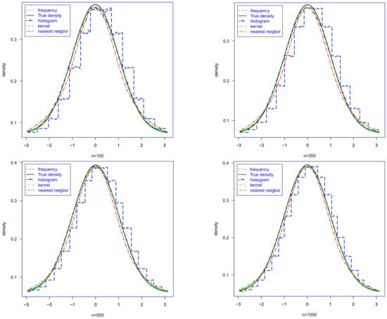
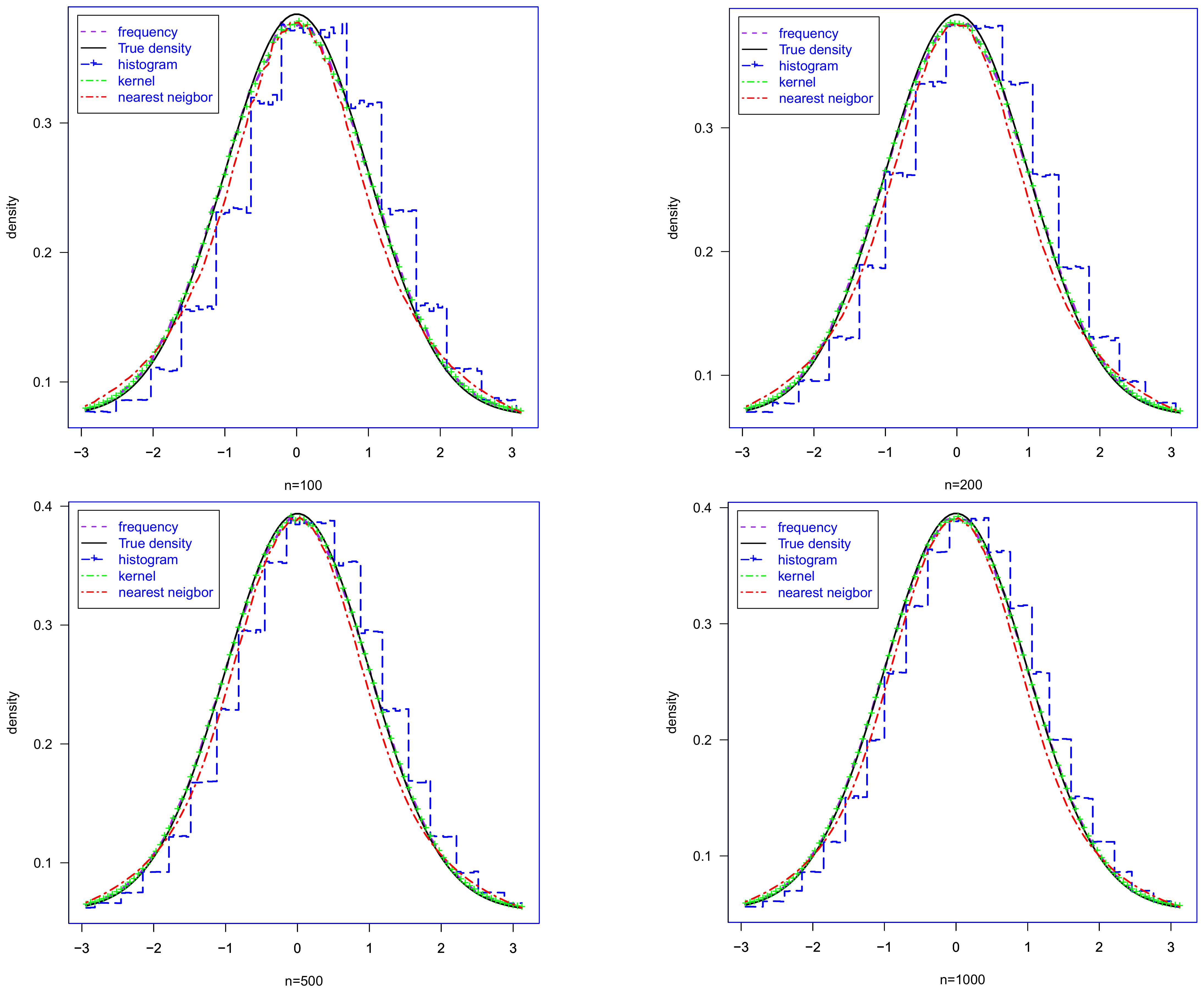
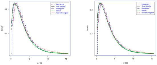
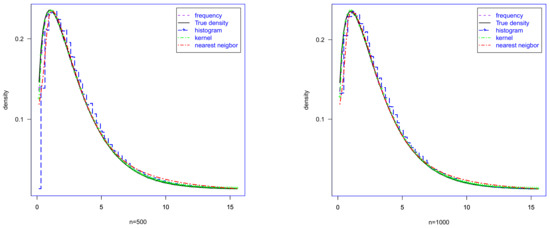
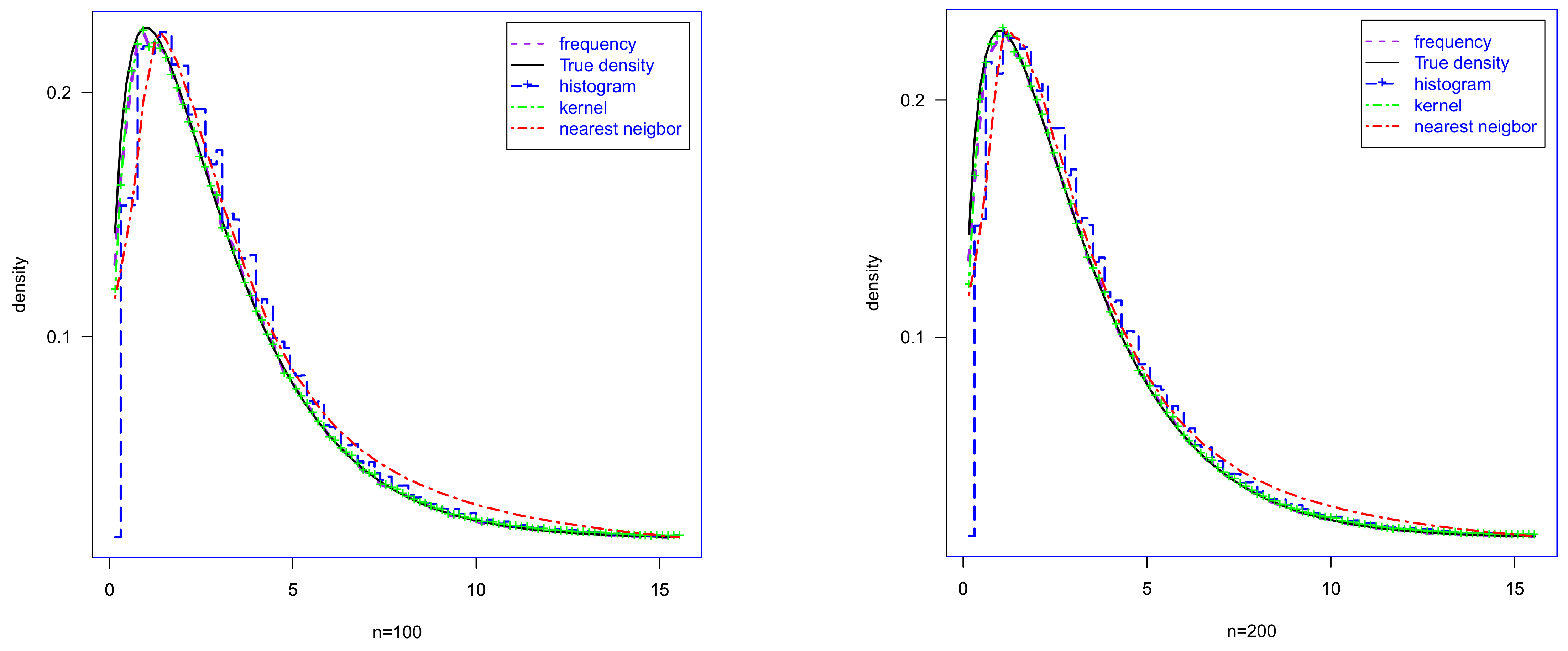
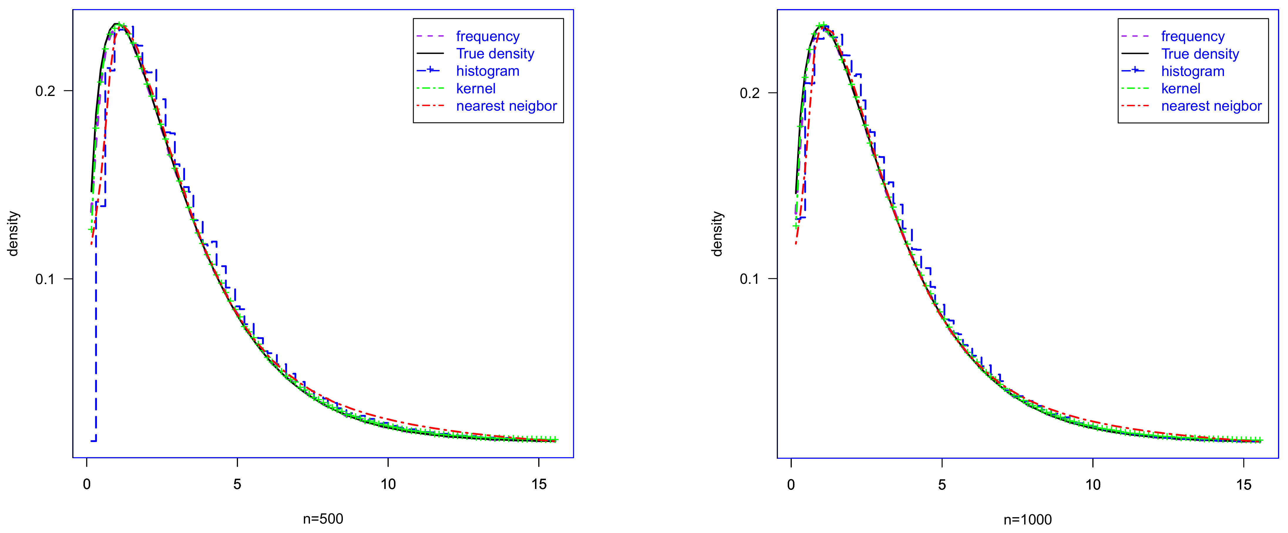
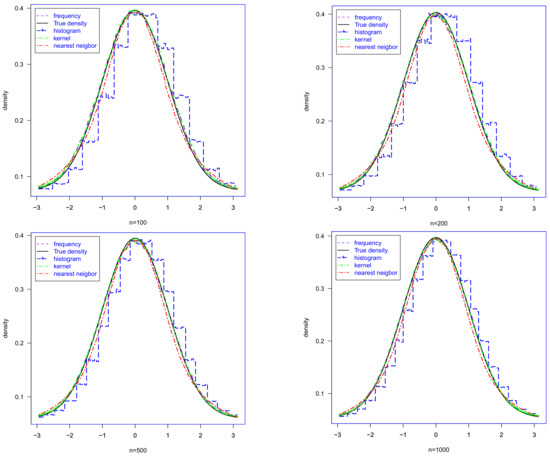
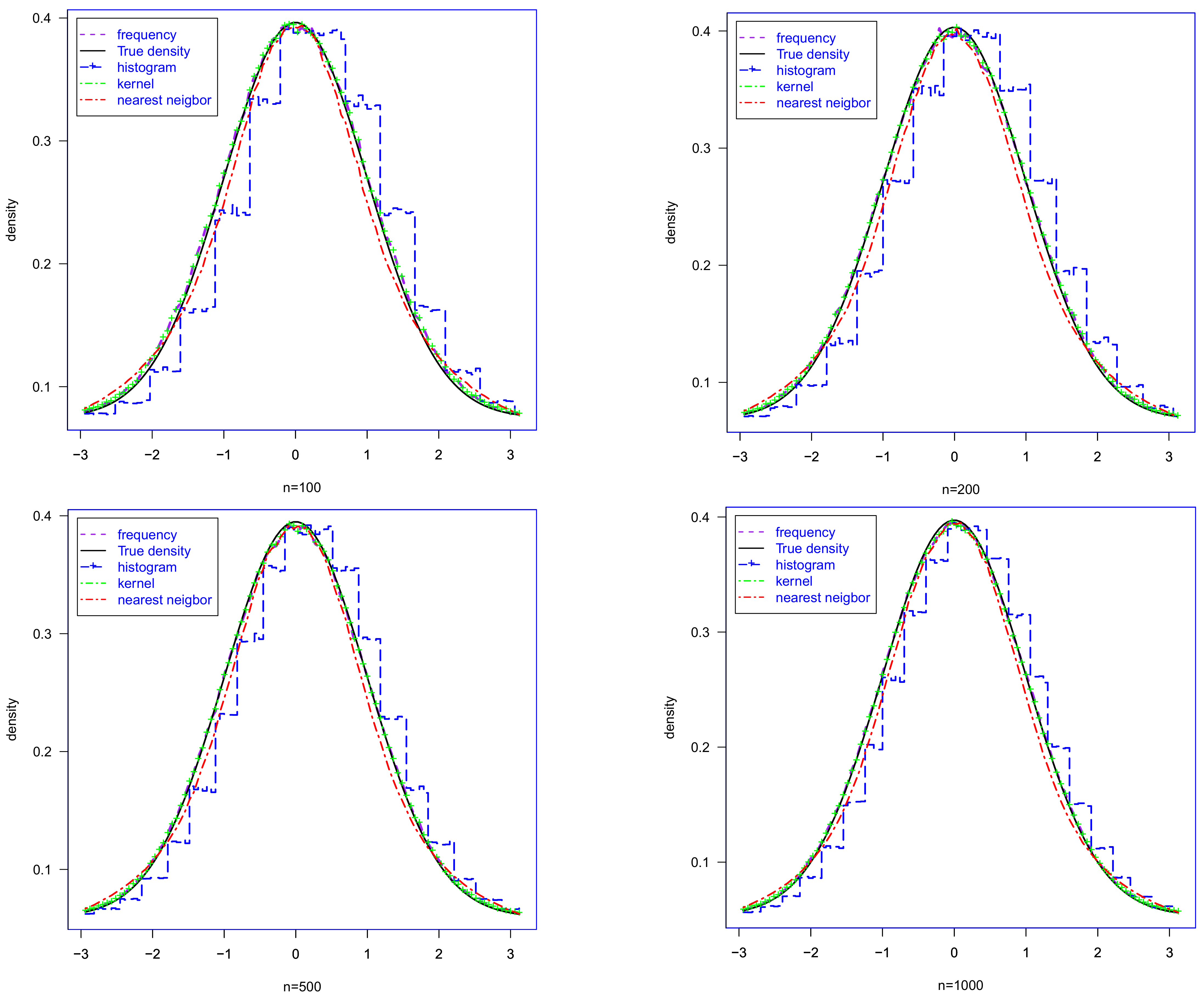
In this section, we will compare the frequency polygon estimator, Epanechnikov kernel estimator (that is, the kernel $K\left(u\right)=0.75(1-u^2)I\left(\right|u|\le 1)$), and histogram estimation with the nearest neighbor estimator. In the sequel, we take $m=3$, $k_n=n^{3/4}{(logn)}^{1/4}$ for the nearest neighbor estimator, the bin-width $b_n={(log\left(n\right)/n)}^{0.25}$ for the frequency polygon estimator and the histogram estimator, and the bandwidth by cross validation (CV, in short) method for the Epanechnikov kernel estimator. It is deserved to mention that $k_n$ and $b_n$ are chosen to achieve the optimal convergence rates. According to the above three cases, we take $n=100,200,500,1000$ and different x-values such as the peak and tail, respectively. For different x and n, we adopt the R software to calculate the four estimators for 1000 times to obtain the the absolute bias (ABias, in short) and the root mean squared error (RMSE, in short) of the four estimators. The conclusions obtained are exhibited in Table 1, Table 2 and Table 3 and Figure 1, Figure 2 and Figure 3.

Table 1. Absolute bias and RMSE of the estimators for different x and n under Case 1.

	Estimators	$\mathit{n}=100$		$\mathit{n}=200$		$\mathit{n}=500$		$\mathit{n}=1000$
		ABias	RMSE	ABias	RMSE	ABias	RMSE	ABias	RMSE
$x=-3$	nearest neighbor	0.07513	0.07521	0.06881	0.06884	0.06062	0.06064	0.05455	0.05456
	frequency	0.00996	0.05338	0.00073	0.00681	0.00049	0.00421	0.00021	0.00345
	kernel	0.00102	0.00827	0.00062	0.00597	0.00055	0.00435	0.00023	0.00306
	histogram	0.00048	0.01018	0.00026	0.00720	0.00170	0.00436	0.00028	0.00377
$x=-2$	nearest neighbor	0.06779	0.06823	0.06132	0.06162	0.05254	0.05268	0.04602	0.04612
	frequency	0.00362	0.02606	0.00361	0.01935	0.00326	0.01296	0.00232	0.01059
	kernel	0.00303	0.02625	0.00232	0.02022	0.00177	0.01357	0.00160	0.01109
	histogram	0.07034	0.03137	0.01985	0.02798	−0.01545	0.02166	0.01523	0.01837
$x=-1$	nearest neighbor	0.00113	0.02717	0.00081	0.02108	0.00053	0.01543	0.00053	0.01263
	frequency	0.00252	0.04723	0.00081	0.04873	0.00067	0.02424	0.00032	0.02708
	kernel	0.00119	0.05112	0.00238	0.03798	0.00161	0.02682	0.00136	0.02187
	histogram	0.03560	0.07545	0.00353	0.053270	0.04199	0.05295	0.00349	0.02816
$x=0$	nearest neighbor	0.02042	0.05259	0.01371	0.04031	0.00963	0.02860	0.00854	0.02147
	frequency	0.01325	0.05293	0.01086	0.04271	0.00658	0.03040	0.00584	0.02284
	kernel	0.00741	0.06047	0.00504	0.04741	0.00359	0.03413	0.00336	0.02526
	histogram	0.01467	0.08489	0.01040	0.06492	0.00689	0.04507	0.00633	0.03474
$x=1$	nearest neighbor	0.00106	0.02738	0.00042	0.02209	0.00015	0.01542	0.00011	0.01206
	frequency	0.00055	0.04615	0.00045	0.04985	0.00040	0.02470	0.00041	0.02743
	kernel	0.00147	0.05031	0.00066	0.03776	0.00044	0.02680	0.00035	0.02131
	histogram	0.07177	0.10530	0.08878	0.10489	0.03915	0.05692	0.06573	0.07274
$x=2$	nearest neighbor	0.06767	0.06812	0.06132	0.06158	0.05256	0.05270	0.04601	0.04610
	frequency	0.00413	0.02620	0.00444	0.01990	0.00340	0.01307	0.00181	0.01024
	kernel	0.00377	0.02602	0.00269	0.02079	0.00214	0.01401	0.00105	0.010646
	histogram	0.05344	0.07064	0.02396	0.03920	0.02081	0.02901	0.01517	0.02162
$x=3$	nearest neighbor	0.07521	0.07528	0.06886	0.06891	0.06056	0.06058	0.05463	0.05464
	frequency	0.00031	0.00954	0.00037	0.00685	0.00073	0.00400	0.00010	0.00338
	kernel	0.00055	0.00775	0.00052	0.00582	0.00050	0.00418	0.00018	0.00306
	histogram	0.01169	0.02231	0.00880	0.01486	0.00289	0.00709	0.00482	0.00742

Table 2. Absolute bias and RMSE of the estimators for different x and n under Case 2.

	Estimators	$\mathit{n}=100$		$\mathit{n}=200$		$\mathit{n}=500$		$\mathit{n}=1000$
		ABias	RMSE	ABias	RMSE	ABias	RMSE	ABias	RMSE
$x=0.5$	nearest neighbor	0.07937	0.08512	0.07047	0.07557	0.06200	0.06529	0.05413	0.05700
	frequency	0.05327	0.06563	0.04324	0.05447	0.03510	0.04427	0.02271	0.02801
	kernel	0.05503	0.06888	0.04300	0.05439	0.02891	0.03614	0.02245	0.02760
	histogram	0.08357	0.09896	0.07807	0.09017	0.07992	0.08971	0.02819	0.03487
$x=1.5$	nearest neighbor	0.03234	0.04047	0.02504	0.03128	0.01759	0.02166	0.01335	0.01664
	frequency	0.04927	0.06188	0.04007	0.05044	0.03334	0.04124	0.01986	0.02491
	kernel	0.04893	0.06156	0.03944	0.04890	0.02663	0.03332	0.02040	0.02552
	histogram	0.06777	0.08469	0.04864	0.06130	0.03455	0.04433	0.02638	0.03333
$x=3.5$	nearest neighbor	0.01586	0.01996	0.01234	0.01603	0.00910	0.01165	0.00705	0.00898
	frequency	0.04376	0.05452	0.03050	0.03800	0.02394	0.02996	0.01349	0.01714
	kernel	0.03614	0.04503	0.02806	0.03482	0.01943	0.02416	0.01475	0.01833
	histogram	0.04599	0.05764	0.03562	0.04456	0.02888	0.03656	0.02029	0.02558
$x=5.5$	nearest neighbor	0.01592	0.01860	0.01238	0.01427	0.00930	0.01061	0.00733	0.00832
	frequency	0.02479	0.03077	0.02090	0.02603	0.01604	0.020318	0.00909	0.01148
	kernel	0.02559	0.03209	0.01918	0.02377	0.01320	0.01662	0.00985	0.01238
	histogram	0.03294	0.04127	0.02325	0.02916	0.01824	0.02381	0.01302	0.01638
$x=7.5$	nearest neighbor	0.02162	0.02211	0.01833	0.01864	0.01465	0.01483	0.01221	0.01235
	frequency	0.01690	0.02115	0.01460	0.01878	0.01023	0.01286	0.00621	0.00784
	kernel	0.01717	0.02170	0.01262	0.01621	0.00861	0.01073	0.00669	0.00840
	histogram	0.02260	0.02991	0.01564	0.02034	0.01209	0.01539	0.00849	0.01072
$x=9.5$	nearest neighbor	0.02283	0.02293	0.02012	0.02019	0.01680	0.01684	0.01441	0.01444
	frequency	0.01327	0.01601	0.00923	0.01197	0.00666	0.00838	0.00386	0.00495
	kernel	0.01026	0.01298	0.00823	0.01044	0.00562	0.00708	0.00416	0.00534
	histogram	0.01335	0.01611	0.00962	0.01247	0.00720	0.00915	0.00518	0.00666

Table 3. Absolute bias and RMSE of the estimators for different x and n under Case 3.

	Estimators	$\mathit{n}=100$		$\mathit{n}=200$		$\mathit{n}=500$		$\mathit{n}=1000$
		ABias	RMSE	ABias	RMSE	ABias	RMSE	ABias	RMSE
$x=-3$	nearest neighbor	0.07610	0.07633	0.06950	0.06971	0.06052	0.06056	0.05461	0.05464
	frequency	0.00930	0.01622	0.00652	0.01128	0.00645	0.00749	0.00496	0.00588
	kernel	0.00832	0.01284	0.00710	0.01021	0.00684	0.00807	0.00444	0.00536
	histogram	0.00815	0.01663	0.00757	0.01188	0.00703	0.00814	0.00563	0.00635
$x=-2$	nearest neighbor	0.06923	0.07070	0.06118	0.06196	0.05715	0.05762	0.04669	0.04682
	frequency	0.03861	0.04881	0.02607	0.03371	0.01926	0.02511	0.01853	0.02361
	kernel	0.03808	0.04823	0.02820	0.03432	0.02276	0.03059	0.01802	0.02188
	histogram	0.04937	0.05914	0.03343	0.03839	0.02003	0.02545	0.01756	0.02350
$x=-1$	nearest neighbor	0.03631	0.04775	0.03392	0.04506	0.01997	0.02303	0.00912	0.00912
	frequency	0.06229	0.07671	0.07247	0.08903	0.02984	0.03644	0.03866	0.03866
	kernel	0.06957	0.08409	0.05274	0.06531	0.02978	0.03729	0.01678	0.01678
	histogram	0.09321	0.08409	0.07434	0.09125	0.05200	0.05696	0.03899	0.03899
$x=0$	nearest neighbor	0.07075	0.08889	0.04916	0.06248	0.04165	0.04875	0.03089	0.03813
	frequency	0.07385	0.09206	0.05638	0.06542	0.05210	0.06610	0.03407	0.04322
	kernel	0.08064	0.10095	0.06331	0.07623	0.06388	0.08090	0.03431	0.04535
	histogram	0.11434	0.14591	0.08077	0.09885	0.06366	0.07957	0.04986	0.06241
$x=1$	nearest neighbor	0.03835	0.05063	0.03149	0.04136	0.02109	0.02732	0.01697	0.02093
	frequency	0.06490	0.08186	0.07414	0.08815	0.03691	0.04265	0.03429	0.04344
	kernel	0.07212	0.09097	0.05512	0.06931	0.03643	0.04574	0.02777	0.03529
	histogram	0.11180	0.14016	0.10962	0.13703	0.06845	0.08603	0.06755	0.08356
$x=2$	nearest neighbor	0.06930	0.07076	0.06486	0.06573	0.05061	0.05079	0.04127	0.04130
	frequency	0.03604	0.04665	0.02133	0.02786	0.01916	0.02315	0.01822	0.01687
	kernel	0.03724	0.04655	0.02060	0.02754	0.01864	0.02148	0.01502	0.01845
	histogram	0.08088	0.10331	0.04690	0.06046	0.02693	0.02977	0.02277	0.02503
$x=3$	nearest neighbor	0.07593	0.07617	0.06940	0.06952	0.06054	0.06056	0.05479	0.05480
	frequency	0.00771	0.01406	0.00754	0.01303	0.00444	0.00444	0.00354	0.00390
	kernel	0.00831	0.01153	0.00781	0.01102	0.00511	0.00576	0.00350	0.00388
	histogram	0.02136	0.03534	0.01559	0.02350	0.00573	0.00655	0.01239	0.01605

Figure 1. Comparison of different estimators for $n=100,200,500,1000$ under case 1.

Figure 2. Comparison of different estimators for $n=100,200,500,1000$ under case 2.

Figure 3. Comparison of different estimators for $n=100,200,500,1000$ under case 3.

In view of Table 1, Table 2 and Table 3 and Figure 1, Figure 2 and Figure 3, we can see the same conclusion under the three cases. Firstly, as the sample size increases, the error of all estimators decreases. The nearest neighbour estimator performs a little better than the kernel estimator and histogram estimation at most points, while at the points distributed on the tail, the nearest neighbour estimator performs worse than the later ones. In summary, the nearest neighbour estimator performs better than others near the peak but worse near the tail. These results show that the estimator considered in this paper also has some superiority to other classical estimators under dependent settings.

5. Proof of the Main Results

The proofs are similar to those of Wu and Wang [15]. Therefore, we only present the differences in the sequel.

Proof of Theorem 1.

Similar to the proof of Wu and Wang [15], we have

$$\begin{array}{c}\hfill \left\{\right|f_n\left(x\right)-f\left(x\right)|>\epsilon \}\subset A_{11x}\bigcup A_{12x}\bigcup A_{21x}\bigcup A_{22x},\end{array}$$

(7)

where

$$\begin{array}{c}\hfill A_{11x}=\left\{|F_n(x+b_n\left(x\right))-F(x+b_n\left(x\right))|\ge \frac{k_n}{n}\delta \left(x\right)\right\},\end{array}$$

$$\begin{array}{c}\hfill A_{12x}=\left\{|F_n(x-b_n\left(x\right))-F(x-b_n\left(x\right))|\ge \frac{k_n}{n}\delta \left(x\right)\right\},\end{array}$$

$$\begin{array}{c}\hfill A_{21x}=\left\{|F_n(x+c_n\left(x\right))-F(x+c_n\left(x\right))|\ge \frac{k_n}{n}\delta \left(x\right)\right\},\end{array}$$

and

$$\begin{array}{c}\hfill A_{22x}=\left\{|F_n(x-c_n\left(x\right))-F(x-c_n\left(x\right))|\ge \frac{k_n}{n}\delta \left(x\right)\right\}\end{array}$$

with $\delta \left(x\right)=\frac{\epsilon }{8\left(f\right(x)+\epsilon )}$.

For given x, define for each $1\le i\le n,n\ge 1$ that

$$\begin{array}{c}\hfill {\xi }_{ni}=I(X_i<x+b_n\left(x\right))-EI(X_i<x+b_n\left(x\right)).\end{array}$$

From Lemma 2, it is easy to see that ${\xi }_{n1},{\xi }_{n2},\dots ,{\xi }_{nn}$ are still m-AANA random variables with $E{\xi }_{ni}=0$ and $|{\xi }_{ni}|\le 1$. Observe that $k_n\le n$ and $\delta \left(x\right)\le \frac{1}{8}$. Using Lemma 4, we have that

$$\begin{array}{ccc}\hfill P\left(A_{11x}\right)& =& P\left(|F_n(x+b_n\left(x\right))-F(x+b_n\left(x\right))|\ge \frac{k_n}{n}\delta \left(x\right)\right)\hfill \\ & =& P\left(\left|\sum _{k=1}^n{\xi }_{ni}\right|>k_n\delta \left(x\right)\right)\hfill \\ & \le & C{\chi }_n·exp\left\{-\frac{k_n^2{\delta }^2\left(x\right)/m^2}{2B_n^2+\frac{2}{3}{k}_n\delta \left(x\right)/m}\right\}\hfill \\ & \le & C{\chi }_n·exp\left\{-\frac{k_n^2{\delta }^2\left(x\right)/m^2}{2n+\frac{1}{12}n/m}\right\}\hfill \\ & =& C{\chi }_n·exp\left\{-\frac{12{\delta }^2\left(x\right)/m}{24m+1}\frac{k_n^2}{n}\right\}.\hfill \end{array}$$

(8)

Analogously, we can also obtain the same upper bounds as in (8) for the probability of events $A_{12x}$, $A_{21x}$, and $A_{22x}$, respectively. Therefore, we further obtain by (5) and (7) that

$$\begin{array}{ccc}\hfill P\left(\right|f_n\left(x\right)-f\left(x\right)|>\epsilon )& \le & P\left(A_{11x}\right)+P\left(A_{12x}\right)+P\left(A_{21x}\right)+P\left(A_{22x}\right)\hfill \\ & \le & 4C{\chi }_n·exp\left\{-\frac{12{\delta }^2\left(x\right)/m}{24m+1}\frac{k_n^2}{n}\right\}\to 0.\hfill \end{array}$$

The proof is finished. □

Proof of Corollary 1.

In view of Theorem 1, we only need to verify that (5) holds. By $k_n^2/(nlogn)\to \infty$, one can obtain that

$$\begin{array}{c}\hfill exp\left\{-\frac{\gamma k_n^2}{n}\right\}\le exp\{-3logn\}=n^{-3}\end{array}$$

(9)

for any $\gamma >0$ and any sufficiently large n. Moreover, noticing that $q\left(n\right)\to 0$, $n_0>0$ exists such that $q\left(n\right)\le 1$ for all $n>n_0$, and thus

$$\begin{array}{c}\hfill {\chi }_n=\sum _{k=1}^{n-1}q\left(k\right)+1=O\left(n\right).\end{array}$$

Therefore, we have by (9) that

$$\begin{array}{c}\hfill {\chi }_{n}exp\left\{-\frac{\gamma k_n^2}{n}\right\}\le C{n}^{-2}\to 0,\end{array}$$

(10)

which finishes the proof. □

Proof of Theorem 2.

The proof is analogous to that of Theorem 1. In view of (6), one has that

$$\begin{array}{c}\hfill \sum _{n=1}^{\infty }P\left(\right|f_n\left(x\right)-f\left(x\right)|>\epsilon )\le 4C\sum _{n=1}^{\infty }{\chi }_n·exp\left\{-\frac{12{\delta }^2\left(x\right)/m}{24m+1}\frac{k_n^2}{n}\right\}<\infty .\end{array}$$

Hence, the desired result follows from the Borel–Cantelli lemma and the formula above immediately. □

Proof of Corollary 2.

Similar to the proof of Corollary 1, we have by (10) that

$$\begin{array}{c}\hfill \sum _{n=1}^{\infty }\left[\sum _{k=1}^{n-1}q\left(k\right)+1\right]·exp\left\{-\frac{\gamma k_n^2}{n}\right\}\le C\sum _{n=1}^{\infty }{n}^{-2}<\infty .\end{array}$$

The proof is thus finished. □

Proof of Theorem 3.

Analogous to the proof of Theorem 2.6 in Wu and Wang [15], we also have that

$$\begin{array}{c}\hfill \left\{\right|f_n\left(x\right)-f\left(x\right)|>D{\tau }_n\}\subset B_{11x}\bigcup B_{12x}\bigcup B_{21x}\bigcup B_{22x},\end{array}$$

(11)

where

$$\begin{array}{c}\hfill B_{11x}=\left\{|F_n(x+{\mu }_n\left(x\right))-F(x+{\mu }_n\left(x\right))|\ge \frac{k_n{\tau }_n}{n}·\frac{D}{8T}\right\},\end{array}$$

$$\begin{array}{c}\hfill B_{12x}=\left\{|F_n(x-{\mu }_n\left(x\right))-F(x-{\mu }_n\left(x\right))|\ge \frac{k_n{\tau }_n}{n}·\frac{D}{8T}\right\},\end{array}$$

$$\begin{array}{c}\hfill B_{21x}=\left\{|F_n(x+{\nu }_n\left(x\right))-F(x+{\nu }_n\left(x\right))|\ge \frac{k_n{\tau }_n}{n}·\frac{D}{8T}\right\},\end{array}$$

and

$$\begin{array}{c}\hfill B_{22x}=\left\{|F_n(x-{\nu }_n\left(x\right))-F(x-{\nu }_n\left(x\right))|\ge \frac{k_n{\tau }_n}{n}·\frac{D}{8T}\right\}\end{array}$$

with $T=:{sup}_{x}f\left(x\right)<\infty$, $D>\frac{c_1^{2}L\left(x\right)}{f\left(x\right)}$ and $L\left(x\right)>0$ depending only on x.

For each given x and $1\le i\le n,n\ge 1$, we define

$$\begin{array}{c}\hfill {\eta }_{ni}=I(X_i<x+{\mu }_n\left(x\right))-EI(X_i<x+{\mu }_n\left(x\right)).\end{array}$$

From Lemma 2, it is easy to see that ${\eta }_{n1},{\eta }_{n2},\dots ,{\eta }_{nn}$ are still m-AANA random variables with $E{\eta }_{ni}=0$ and $|{\eta }_{ni}|\le 1$. Applying Lemma 4 and noticing that $k_n\le n$, ${\tau }_n\to 0$, we obtain that for all sufficiently large n,

$$\begin{array}{ccc}\hfill P\left(B_{11x}\right)& =& P\left(|F_n(x+{\mu }_n\left(x\right))-F(x+{\mu }_n\left(x\right))|\ge \frac{k_n{\tau }_n}{n}·\frac{D}{8T}\right)\hfill \\ & =& P\left(\left|\sum _{i=1}^n{\eta }_{ni}\right|>k_n{\tau }_n·\frac{D}{8T}\right)\hfill \\ & \le & C{\chi }_n·exp\left\{-\frac{k_n^2{\tau }_n^2{D}^2/\left(64T^2{m}^2\right)}{2B_n^2+\frac{D}{12Tm}{k}_n{\tau }_n}\right\}\hfill \\ & \le & Cnexp\left\{-\frac{k_n^2{\tau }_n^2}{n}·\frac{D^2}{128m^2{T}^2+\frac{16}{3}DmT}\right\}\hfill \\ & =& Cnexp\left\{-\frac{D^2}{128m^2{T}^2+\frac{16}{3}DmT}logn\right\}\hfill \\ & \le & C{n}^{1-\frac{D^2}{128m^2{T}^2+\frac{16}{3}DmT}}.\hfill \end{array}$$

(12)

Analogously, the probabilities of $B_{12x}$, $B_{21x}$, and $B_{22x}$ also have the same upper bounds as in (12). Therefore, taking $D>\frac{c_0^{2}L\left(x\right)}{f\left(x\right)}$ such that $1-\frac{D^2}{128m^2{T}^2+\frac{16}{3}DmT}<-1$, one can obtain by (11) that

$$\begin{array}{ccc}\hfill \sum _{n=1}^{\infty }P\left(\right|f_n\left(x\right)-f\left(x\right)|>D{\tau }_n)& \le & \sum _{n=1}^{\infty }(P\left(B_{11x}\right)+P\left(B_{12x}\right)+P\left(B_{21x}\right)+P\left(B_{22x}\right))\hfill \\ & \le & 4C\sum _{n=1}^{\infty }{n}^{1-\frac{D^2}{128m^2{T}^2+\frac{16}{3}DmT}}<\infty .\hfill \end{array}$$

This completes the proof of the theorem. □

Proof of Theorem 4.

It follows from the proof of Theorem 2.9 in Wu and Wang [15] that

$$\begin{array}{c}\hfill \left(\underset{x}{sup}|f_n\left(x\right)-f\left(x\right)|>\epsilon \right)\subset \left(\underset{x}{sup}|F_n\left(x\right)-F\left(x\right)|\ge \frac{\epsilon }{8(T+\epsilon )}\frac{k_n}{n}\right),\end{array}$$

(13)

where $T={sup}_{x}f\left(x\right)<\infty$.

On the other hand, by $k_n^2/(nlogn)\to \infty$ we have that for all sufficiently large n, $\frac{\epsilon }{8(T+\epsilon )}\frac{k_n}{n}\ge D_0{(logn/n)}^{1/2}$. Hence, taking ${\kappa }_n={(logn/n)}^{1/2}$ in Lemma 6, one has by (13) that

$$\begin{array}{ccc}\hfill \sum _{n=1}^{\infty }P\left(\underset{x}{sup}|f_n\left(x\right)-f\left(x\right)|>\epsilon \right)& \le & \sum _{n=1}^{\infty }P\left(\underset{x}{sup}|F_n\left(x\right)-F\left(x\right)|\ge \frac{\epsilon }{8(T+\epsilon )}\frac{k_n}{n}\right)\hfill \\ & \le & \sum _{n=1}^{\infty }P\left(\underset{x}{sup}|F_n\left(x\right)-F\left(x\right)|\ge D_0{(logn/n)}^{1/2}\right)<\infty .\hfill \end{array}$$

The proof is hence finished. □

Proof of Theorem 5.

It follows from the proof of Theorem 2.10 in Wu and Wang [15] that

$$\begin{array}{c}\hfill \left(\underset{x}{sup}|f_n\left(x\right)-f\left(x\right)|>D{\tau }_n\right)\subset \left(\underset{x}{sup}|F_n\left(x\right)-F\left(x\right)|\ge \frac{k_n{\tau }_n}{n}·\frac{D}{8T}\right),\end{array}$$

(14)

where $D>max\{\sqrt{4c_2^{3}L},8T{D}_0\}$, $T={sup}_{x}f\left(x\right)<\infty$, and $L>0$ is independent of x.

Consequently, on can apply Lemma 6 with ${\kappa }_n=\frac{k_n{\tau }_n}{n}={(logn/n)}^{1/2}$ to obtain that

$$\begin{array}{ccc}\hfill \sum _{n=1}^{\infty }P\left(\underset{x}{sup}|f_n\left(x\right)-f\left(x\right)|>D{\tau }_n\right)& \le & \sum _{n=1}^{\infty }P\left(\underset{x}{sup}|F_n\left(x\right)-F\left(x\right)|\ge \frac{k_n{\tau }_n}{n}·\frac{D}{8T}\right)\hfill \\ & \le & \sum _{n=1}^{\infty }P\left(\underset{x}{sup}|F_n\left(x\right)-F\left(x\right)|\ge D_0{(logn/n)}^{1/2}\right)<\infty .\hfill \end{array}$$

This completes the proof of the theorem. □

6. Conclusions

In this paper, a Bernstein inequality for m-asymptotically almost negatively associated random variables is established based on that of asymptotically almost negatively associated random variables. By virtue of this inequality, some results on consistency for the nearest neighbor estimator of the density function are further obtained. The results are further extensions of existing ones in the literature. From the simulation study, we find that the nearest neighbour estimator performs better than others on the peak but worse on the tail, which encourages us to consider whether we can combine the superiorities of these estimators to construct a better method.

References

- Loftsgarden, D.O.; Quesenberry, C.P. A nonparametric estimate of a multivariate density function. Ann. Math. Stat. 1965, 36, 1049–1051. [Google Scholar] [CrossRef] [Scilit]
- Liu, Y.H.; Wu, Q.Y. Consistency of nearest neighbor estimator of density function for negatively dependent samples. J. Jilin Univ. 2012, 50, 1142–1145. [Google Scholar]
- Lu, Z.L.; Ding, S.N.; Zhang, F.; Wang, R.; Wang, X.J. The consistency and convergence rate for the nearest neighbor density estimator based on φ-mixing random samples. Commun. Stat.-Theory Methods 2022, 51, 669–684. [Google Scholar] [CrossRef] [Scilit]
- Liu, Y.; Zhang, Y. The consistency and asymptotic normality of nearest neighbor density estimator under φ-mixing condition. Acta Math. Sin. 2010, 30, 733–738. [Google Scholar]
- Yang, S.C. Consistency of nearest neighbor estimator of density function for negative associated samples. Acta Math. Appl. Sin. 2003, 26, 385–395. [Google Scholar]
- Wang, X.J.; Hu, H.S. The consistency of the nearest neighbor estimator of the density function based on WOD samples. J. Math. Anal. Appl. 2015, 429, 497–512. [Google Scholar] [CrossRef] [Scilit]
- Lan, C.F.; Wu, Q.Y. Uniform Strong Consistency Rate of Nearest Neighbor Estimator of Density Function for END Samples. J. Jilin Univ. 2014, 52, 495–498. [Google Scholar]
- Wang, W.; Wu, Y. Consistency of nearest neighbor estimator of density function for m-END samples. Braz. J. Probab. Stat. 2022, 36, 369–384. [Google Scholar] [CrossRef] [Scilit]
- Chandra, T.K.; Ghosal, S. Extensions of the strong law of large numbers of Marcinkiewicz and Zygmund for dependent variables. Acta Math. Hung. 1996, 71, 327–336. [Google Scholar] [CrossRef] [Scilit]
- Kim, T.; Ko, M.; Lee, I. On the strong law for asymptotically almost negatively associated random variables. Rocky Mt. J. Math. 2004, 34, 979–989. [Google Scholar] [CrossRef] [Scilit]
- Yuan, D.M.; An, J. Rosenthal type inequalities for asymptotically almost negatively associated random variables and applications. Sci. China Ser. A Math. 2009, 52, 1887–1904. [Google Scholar] [CrossRef] [Scilit]
- Chandra, T.K.; Ghosal, S. The strong law of large numbers for weighted averages under dependence assumptions. J. Theor. Probab. 1996, 9, 797–809. [Google Scholar] [CrossRef] [Scilit]
- Shen, A.T.; Wu, R.C. Strong convergence for sequences of asymptotically almost negatively associated random variables. Stochastics-Int. J. Probab. Stoch. Process. 2014, 86, 291–303. [Google Scholar] [CrossRef] [Scilit]
- Yuan, D.M.; An, J. Laws of large numbers for Cesàro alpha-integrable random variables under dependence condition AANA or AQSI. Acta Math. Sin. 2012, 28, 1103–1118. [Google Scholar] [CrossRef] [Scilit]
- Wu, Y.; Wang, X.J. On Consistency of the Nearest Neighbor Estimator of the Density Function and Its Applications. Acta Math. Sin. 2019, 35, 703–720. [Google Scholar] [CrossRef] [Scilit]
- Nam, T.H.; Thuy, N.T.; Hu, T.C.; Volodin, A. Maximal inequalities and strong law of large numbers for sequences of m-asymptotically almost negatively associated random variables. Commun. Stat.-Theory Methods 2016, 46, 2696–2707. [Google Scholar] [CrossRef] [Scilit]
Disclaimer/Publisher’s Note: The statements, opinions and data contained in all publications are solely those of the individual author(s) and contributor(s) and not of MDPI and/or the editor(s). MDPI and/or the editor(s) disclaim responsibility for any injury to people or property resulting from any ideas, methods, instructions or products referred to in the content. |
© 2023 by the authors. Licensee MDPI, Basel, Switzerland. This article is an open access article distributed under the terms and conditions of the Creative Commons Attribution (CC BY) license (https://creativecommons.org/licenses/by/4.0/).