General Odd and Even Central Factorial Polynomial Sequences

Abstract

The ${\delta }^2(·)$ operator, where $\delta (·)$ is the known central difference operator, is considered. The associated odd and even polynomial sequences are determined and their generalizations studied. Particularly, matrix and determinant forms, recurrence formulas, generating functions and an algorithm for effective calculation are provided. An interesting property of biorthogonality is also demonstrated. New examples of odd and even central polynomial sequences are given.

1. Introduction

Polynomials are very useful mathematical tools, as they are defined in a simple way and they can be easily differentiated and integrated. Moreover, they can be quickly calculated on a computer system and are used to form spline functions.

One of the main problems in applied mathematics is the computation of real functions. In general, functions that are given as integro-differential equations cannot be explicitly expressed in terms of the so-called elementary functions. In addition, even elementary functions can take real values that cannot be explicitly given.

For these reasons, we often need to approximate a given function using simpler functions. In 1885, Weierstass [1] proved the approximation theorem according to which any continuous function defined on a closed and bounded interval can be uniformly approximated by a polynomial function. After this theorem, sets or sequences of polynomials were increasingly studied (see, for example, Refs. [2,3]).

Therefore, we find classes of polynomials in different sciences. For example, orthogonal polynomials are frequently used in physics, in the approximation theory [4,5,6] and also in the solution of differential equations. Hermite polynomials are used in statistics—umbral polynomials in algebra and combinatorics. Particularly, binomial, Appell and Sheffer polynomials are widely used, including more important families as Bernoulli, Euler, Boile, falling factorials, etc. (see [7,8,9,10,11,12] and the references therein).

In [13], Lidstone generalized an Aitken theorem on interpolation and proposed a two-point expansion of polynomials, in which the polynomial basis, called Lidstone polynomials, is expressed in powers of odd and, respectively, even canonical monomials. After, in [14,15], the authors generalized Lidstone polynomials, introduced odd and even special polynomial sequences and gave some applications to approximation functions, boundary value problems and cubature formulas.

In this paper, we consider other odd and even special polynomial sequences that are connected to the ${\delta }^2(·)$ operator, with $\delta (·)$ being the central factorial difference operator ([16], p. 7). These polynomials can be the basis for generalized interpolation Everett-type formulas.

The outline of this paper is as follows. In Section 2, we give some preliminary definitions, results and characterizations, and we formalize the problem; in Section 3, we consider general odd central factorial polynomial sequences and, in Section 4, we consider general even central factorial polynomial sequences. For each kind of sequence (odd and even), we give the matrix form, the conjugate polynomials, recurrence relations and the related determinant forms, the generating function. Finally, we give some examples of new odd and even polynomial sequences. Concluding remarks close the paper.

We will adopt the following abbreviations:

p.s. polynomial sequence
OLPS: odd Lidstone-type p.s.,	ELPS: even Lidstone-type p.s.,
GOCPS: general odd central factorial p.s.,	GECPS: general even central factorial p.s.,
$\widetilde{GOCPS}$: the algebra $\left(GOCPS,+,·,\circ \right),$	$\widetilde{GECPS}$: the algebra $\left(GECPS,+,·,\circ \right)$.

2. Preliminaries and Problem’s Position

In order to make the work as autonomous as possible, we give some preliminary definitions and propositions.

Let ${\left\{p_n\right\}}_{n\in \mathrm{I}\mathrm{N}}$ be a polynomial sequence (p.s. in the following) [17], such that $p_0\left(x\right)=1$ and, for $n\ge 1$, $p_n$ is a polynomial of degree n on a field $\mathrm{I}\mathrm{K}$ of characteristic 0 (typically $\mathrm{I}\mathrm{K}=\mathrm{I}\mathrm{R}$ or $\mathrm{I}\mathrm{K}=ℂ$).

Definition 1.

A polynomial sequence is called symmetric if and only if

$$\forall n\in \mathrm{I}\mathrm{N},\forall x\in \mathrm{I}\mathrm{K},p_n\left(-x\right)={\left(-1\right)}^n{p}_n\left(x\right).$$

(1)

Proposition 1.

Let ${\left\{p_n\right\}}_{n\in \mathrm{I}\mathrm{N}}$ be a symmetric p.s. Then, for all $n\in \mathrm{I}\mathrm{N}$, $p_n$ has the decomposition in classical monomial basis only with powers $x^{n-2k},k=0,1,\dots ,\lfloor \frac{n}{2}\rfloor$.

Proof. 

If we set

$$p_n\left(x\right)=\sum _{k=0}^n{t}_{n,k}{x}^k,t_{n,k}\in \mathrm{I}\mathrm{K},t_{n,n}\ne 0,k=0,\dots ,n,$$

the result follows from (1). □

This suggests us to give the following definition.

Definition 2.

An odd (resp. even) polynomial sequence is a polynomial sequence whose elements have only odd (resp. even) powers in the canonical decomposition.

Of course, a symmetric polynomial involves lower computational costs than a polynomial of the same degree. Moreover, every polynomial of an odd (resp. even) p.s. is an odd (resp. even) function.

In [14,15], the authors consider the so-called odd and, respectively, even Lidstone-type polynomial sequences.

We remember that

(a)

${\left\{p_n\right\}}_{n\in \mathrm{I}\mathrm{N}}$ is an odd Lidstone-type p.s. (OLPS) if and only if

$$\left\{\begin{array}{c}{p}_n^{″}\left(x\right)=2n\left(2n+1\right)p_{n-1}\left(x\right)\hfill \\ p_n\left(0\right)=0,deg\left(p_n\right)=2n+1,n\ge 0.\hfill \end{array}\right.$$

(2)

(b)

${\left\{p_n\right\}}_{n\in \mathrm{I}\mathrm{N}}$ is an even Lidstone-type p.s. (ELPS) if and only if

$$\left\{\begin{array}{c}{p}_n^{″}\left(x\right)=2n\left(2n-1\right)p_{n-1}\left(x\right)\hfill \\ p_n^{\prime }\left(0\right)=0,deg\left(p_n\right)=2n,n\ge 0.\hfill \end{array}\right.$$

(3)

In [15], some applications of OLPS and ELPS were proposed.

Now, we observe that the central factorial polynomials ([17], p. 67), ([18], p. 212), Refs. [19,20], ([16], p. 6) are classically denoted by $x^{\left[n\right]}$ and are defined as

$$\begin{array}{ll}\hfill x^{\left[0\right]}& =1,\hfill \\ \hfill x^{\left[n\right]}& =x\prod _{j=1}^{n-1}\left(x+\frac{n}{2}-j\right),n\ge 1.\hfill \end{array}$$

They satisfy the identity

$$\delta x^{\left[n\right]}=n{x}^{[n-1]},n\ge 1,$$

where $\delta$ is the central operator ([16], p. 7) defined by

$$\delta f\left(x\right)=f\left(x+\frac{1}{2}\right)-f\left(x-\frac{1}{2}\right),$$

with f being a real function of a real variable.

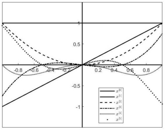
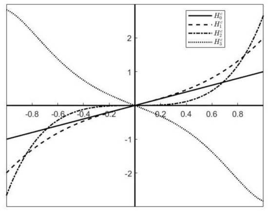
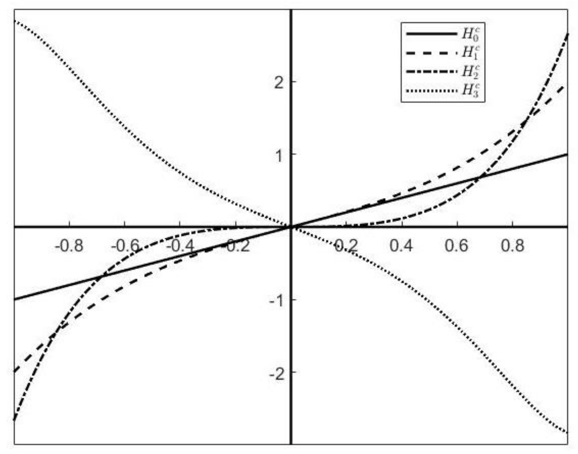
The first of these polynomials are

$$\begin{array}{cc}{x}^{\left[0\right]}=1,\hfill & x^{\left[1\right]}=x,\hfill \\ x^{\left[2\right]}=x^2,\hfill & {\displaystyle x^{\left[3\right]}=x^3-\frac{1}{4}x,}\hfill \\ x^{\left[4\right]}=x^4-x^2,\hfill & {\displaystyle x^{\left[5\right]}=x^5-\frac{5}{2}{x}^3+\frac{9}{16}x.}\hfill \end{array}$$

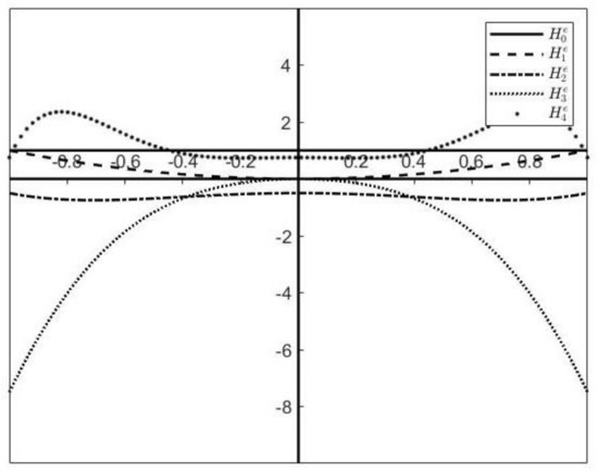
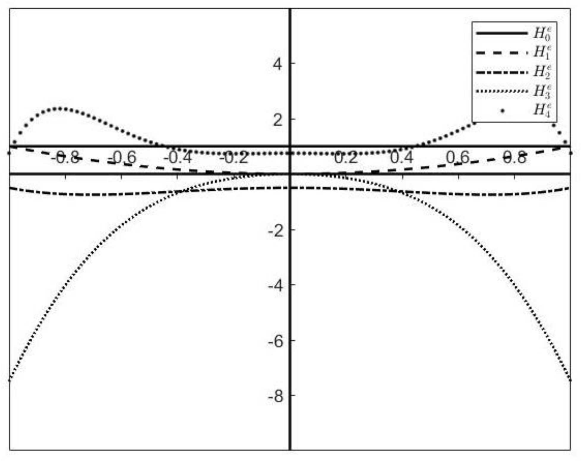
Their plots are shown in Figure 1. The figure was made using Matlab/Octave software.

Figure 1. Central factorial polynomials.

In general, it results in ([16], p. 9)

$${\displaystyle x^{[2\nu +1]}=x\left(x^2-\frac{1}{4}\right)\left(x^2-\frac{9}{4}\right)\dots \left(x^2-\frac{{\left(2\nu -1\right)}^2}{4}\right),}$$

(4a)

$${\displaystyle x^{\left[2\nu \right]}=x^2\left(x^2-1\right)\dots \left(x^2-{\left(\nu -1\right)}^2\right).}$$

(4b)

Remark 1.

It is known that ${\left\{x^{\left[\nu \right]}\right\}}_{\nu \in \mathrm{I}\mathrm{N}}$ is a binomial type sequence ([17], p. 66). It has the following decomposition:

$$x^{\left[\nu \right]}=\sum _{k=0}^{\nu }{b}_{\nu ,k}{x}^k,\forall \nu \in \mathrm{I}\mathrm{N},$$

where the $b_{\nu ,k}$ are calculated by Algorithm 2.1.1 in ([17], p. 7).

In the literature (see for example [17,18,19] and references therein), the numbers $b_{\nu ,k}$ are denoted by $t(\nu ,k)$ and are called central factorial numbers of the first kind. There is a wide amount of literature on these numbers (see, for example, [17,21,22,23,24,25,26] and references therein).

We note that the elements of the subsequence ${\left\{x^{[2\nu +1]}\right\}}_{\nu \in \mathrm{I}\mathrm{N}}$ satisfy the following properties:

(1o)

$x^{[2\nu +1]}$ contains only odd powers of the variable x and $deg{x}^{[2\nu +1]}=2\nu +1$;

(2o)

${\displaystyle {\delta }^2{x}^{[2\nu +1]}=\delta \left(\delta x^{[2\nu +1]}\right)=2\nu (2\nu +1)x^{[2\nu -1]}}$;

(3o)

${\displaystyle x^{[2\nu +1]}\left(0\right)=0,x^{[2\nu +1]}\left(\frac{1}{2}\right)=0,\nu \ge 1}$.

Similarly, the elements of the subsequence ${\left\{x^{\left[2\nu \right]}\right\}}_{\nu \in \mathrm{I}\mathrm{N}}$ satisfy:

(1e)

$x^{\left[2\nu \right]}$ contains only even powers of the variable x and $deg{x}^{\left[2\nu \right]}=2\nu$;

(2e)

${\displaystyle {\delta }^2{x}^{\left[2\nu \right]}=\delta \left(\delta x^{\left[2\nu \right]}\right)=2\nu \delta x^{[2\nu -1]}=2\nu (2\nu -1)x^{[2\nu -2]}}$;

(3e)

${\displaystyle x^{\left[2\nu \right]}\left(0\right)=0,{\left(x^{\left[2\nu \right]}\right)}^{\prime }\left(0\right)=0,x^{\left[2\nu \right]}\left(1\right)=0,\nu \ge 1}$.

Hence, the subsequences ${\left\{x^{[2\nu +1]}\right\}}_{\nu \in \mathrm{I}\mathrm{N}}$ and ${\left\{x^{\left[2\nu \right]}\right\}}_{\nu \in \mathrm{I}\mathrm{N}}$ are respectively an odd and an even p.s. We call the subsequences ${\left\{x^{[2\nu +1]}\right\}}_{\nu \in \mathrm{I}\mathrm{N}}$ and ${\left\{x^{\left[2\nu \right]}\right\}}_{\nu \in \mathrm{I}\mathrm{N}}$ odd and even central factorial p.s., respectively.

The previous considerations suggest generalizing the problem: we look for, if there exists, the odd p.s. ${\left\{d_n\right\}}_{n\in \mathrm{I}\mathrm{N}}$ such that

$$\left\{\begin{array}{c}{\delta }^2{d}_n\left(x\right)=2n\left(2n+1\right)d_{n-1}\left(x\right),n\ge 1,\hfill \\ d_n\left(0\right)=0,deg\left(d_n\right)=2n+1,n\ge 0.\hfill \end{array}\right.$$

(5)

Analogously, we look for, if there exists, the even p.s. ${\left\{e_n\right\}}_{n\in \mathrm{I}\mathrm{N}}$ such that

$$\left\{\begin{array}{c}{\delta }^2{e}_n\left(x\right)=2n\left(2n-1\right)e_{n-1}\left(x\right),n\ge 1,\hfill \\ e_n^{\prime }\left(0\right)=0,deg\left(e_n\right)=2n,n\ge 0.\hfill \end{array}\right.$$

(6)

If these polynomial sequences exist, we call ${\left\{d_n\right\}}_{n\in \mathrm{I}\mathrm{N}}$ general odd central factorial p.s. (GOCPS) and ${\left\{e_n\right\}}_{n\in \mathrm{I}\mathrm{N}}$ general even central factorial p.s. (GECPS).

Remark 2.

Note that (5) and (6) differ from (2) and (3) in the operator: in (5) and (6), there is the discrete central finite difference operator ${\delta }^2$, while, in (2) and (3), there is the differential operator ${\displaystyle \frac{d^2}{d{x}^2}\equiv D^2}$.

3. General Odd Central Factorial Polynomial Sequences

To study problem (5), proceeding by induction, we note that every term $d_n$ of the sequence ${\left\{d_n\right\}}_{n\in \mathrm{I}\mathrm{N}}$ is determined by the previous term $d_{n-1}$ and a constant. The following proposition provides an explicit expression for $d_n$ in terms of central factorial polynomials.

Proposition 2.

Let ${\left\{d_n\right\}}_{n\in \mathrm{I}\mathrm{N}}$ be an odd p.s. It is a GOCPS, that is, it satisfies (5) if and only if there exists a numerical sequence ${\left({\alpha }_{2n}\right)}_{n\in \mathrm{I}\mathrm{N}}$, with ${\alpha }_0\ne 0$, such that

$$d_n\left(x\right)=\sum _{k=0}^n\left(\genfrac{}{}{0pt}{}{2n+1}{2k+1}\right)\frac{{\alpha }_{2(n-k)}}{2(n-k)+1}{x}^{[2k+1]}.$$

(7)

Proof. 

If (7) holds, from the linearity of the operator ${\delta }^2(·)$ and from property (2o), $d_n$ satisfies

$${\delta }^2{d}_n\left(x\right)=2n(2n+1)d_{n-1}\left(x\right).$$

Moreover, it results in $d_n\left(0\right)=0$, $d_0\left(x\right)={\alpha }_{0}x$ and $deg\left(d_n\right)$ is $2n+1$.

Vice versa, we can obtain the result by mathematical induction, taking into account that every odd polynomial can be expressed as a linear combination of $x^{[2i+1]}$, $i\ge 0$. □

Remark 3.

From (4a), for $k>0$,

$${\left(x^{[2k+1]}\right)}^{\prime }\left(0\right)={(-1)}^k\prod _{i=1}^k\frac{{(2i-1)}^2}{4}.$$

Hence, from (7), for $n>0$ it results in

$$d_n^{\prime }\left(0\right)=\sum _{k=0}^n\left(\genfrac{}{}{0pt}{}{2n+1}{2k+1}\right)\frac{{\alpha }_{2(n-k)}}{2(n-k)+1}{(-1)}^k\prod _{i=1}^k\frac{{(2i-1)}^2}{4}.$$

(8)

Proposition 3.

Let ${\left\{d_n\right\}}_{n\in \mathrm{I}\mathrm{N}}$ be a GOCPS. Then, for $j=0,\dots ,n$, we obtain

(1) 

${\displaystyle {\delta }^{2j}{d}_n\left(x\right)=\frac{(2n+1)!}{\left(2\right(n-j)+1)!}{d}_{n-j}\left(x\right)}$;

(2) 

${\displaystyle {\delta }^{2j+1}{d}_n\left(x\right)=\frac{(2n+1)!}{\left(2\right(n-j)+1)!}\delta d_{n-j}\left(x\right)}$;

(3) 

${\displaystyle {\delta }^{2j}{d}_n\left(0\right)=0,{\delta }^{2j+1}{d}_n\left(0\right)=\frac{(2n+1)!}{\left(2\right(n-j)+1)!}\delta d_{n-j}\left(0\right)}$.

Proof. 

The proof follows easily from (5) after some calculations. □

Corollary 1.

Let ${\left\{d_n\right\}}_{n\in \mathrm{I}\mathrm{N}}$ be a GOCPS. Then, $\forall n,j\in \mathrm{I}\mathrm{N}$ with $j<n$, and we obtain

$$\sum _{k=0}^{2j}\left(\genfrac{}{}{0pt}{}{2j}{k}\right){\left(-1\right)}^k{d}_n(x+j-k)=\frac{(2n+1)!}{\left(2\right(n-j)+1)!}{d}_{n-j}\left(x\right),$$

$$\sum _{k=0}^{2j+1}\left(\genfrac{}{}{0pt}{}{2j+1}{k}\right){\left(-1\right)}^k{d}_n\left(x+j-k+\frac{1}{2}\right)=\frac{(2n+1)!}{\left(2\right(n-j)+1)!}\delta d_{n-j}\left(x\right).$$

Proof. 

The proof follows from Proposition 3 and the known identities on operator $\delta$. □

3.1. Matrix Form

Let ${\left\{d_n\right\}}_{n\in \mathrm{I}\mathrm{N}}$ be the GOCPS related to the numerical sequence ${\left({\alpha }_{2n}\right)}_{n\in \mathrm{I}\mathrm{N}}$, ${\alpha }_0\ne 0$, that is, a p.s. as in Proposition 2. The relation (7) suggests to consider the lower infinite triangular matrix ${\mathbf{V}}_{\infty }=\left(v_{i,j}\right)$ with

$$v_{i,j}=\left\{\begin{array}{lll}\left(\genfrac{}{}{0pt}{}{2i+1}{2j+1}\right)\frac{{\alpha }_{2(i-j)}}{2(i-j)+1},\hfill & & i\ge 0,j=0,1,\dots ,i,\\ 0\hfill & & i<j.\end{array}\right.$$

(9)

We note that ${\mathbf{V}}_{\infty }$ is a Lidstone-type matrix as defined in [14].

Let ${\stackrel{\neg }{\mathbf{X}}}_{\infty }$ and ${\mathbf{D}}_{\infty }$ be the infinite vectors

$${\stackrel{\neg }{\mathbf{X}}}_{\infty }={\left[x^{\left[1\right]},x^{\left[3\right]},\dots ,x^{[2\nu +1]},\dots \right]}^T,{\mathbf{D}}_{\infty }={\left[d_0\left(x\right),d_1\left(x\right),\dots ,d_{\nu }\left(x\right),\dots \right]}^T.$$

Then, from (7), we obtain ${\mathbf{D}}_{\infty }={\mathbf{V}}_{\infty }{\stackrel{\neg }{\mathbf{X}}}_{\infty }$, or, for simplicity,

$$\mathbf{D}=\mathbf{V}\stackrel{\neg }{\mathbf{X}},$$

(10)

where, of course, $\mathbf{D}={\mathbf{D}}_{\infty }$, $\mathbf{V}={\mathbf{V}}_{\infty }$, $\stackrel{\neg }{\mathbf{X}}={\stackrel{\neg }{\mathbf{X}}}_{\infty }$.

If, in (9), we consider $i=0,\dots ,n$, $n\in \mathrm{I}\mathrm{N}$, we obtain the principal submatrix of order $n+1$ of $\mathbf{V}$ that we denote by ${\mathbf{V}}_{\mathbf{n}}$. Analogously, ${\stackrel{\neg }{\mathbf{X}}}_{\mathbf{n}}$ and ${\mathbf{D}}_{\mathbf{n}}$ are the principal subvectors with $n+1$ components of ${\stackrel{\neg }{\mathbf{X}}}_{\infty }$ and ${\mathbf{D}}_{\infty }$, respectively.

Then, from (10),

$${\mathbf{D}}_{\mathbf{n}}={\mathbf{V}}_{\mathbf{n}}{\stackrel{\neg }{\mathbf{X}}}_{\mathbf{n}}.$$

(11)

We call the relation (11) (or (10)) the first matrix form of the GOCPS ${\left\{d_n\right\}}_{n\in \mathrm{I}\mathrm{N}}$.

It is known [14] that the matrix $\mathbf{V}$ can be factorized as

$$\mathbf{V}=\mathbf{W}{\mathbf{T}}_{\mathbf{\alpha }}{\mathbf{W}}^{-\mathbf{1}},$$

where $\mathbf{W}=diag\left\{(2i+1)!|i\ge 0\right\}$ and ${\mathbf{T}}_{\mathbf{\alpha }}$ is the lower triangular Toepliz matrix with elements ${\displaystyle t_{i,j}^{\alpha }=\frac{{\alpha }_{2(i-j)}}{\left(2\right(i-j)+1)!}}$.

The matrix $\mathbf{V}$ is invertible and ${\mathbf{V}}^{-\mathbf{1}}={\left(v_{i,j}^{-1}\right)}_{i,j\in \mathrm{I}\mathrm{N}}$, with

$$v_{i,j}^{-1}=\left\{\begin{array}{lll}\left(\genfrac{}{}{0pt}{}{2i+1}{2j+1}\right)\frac{{\beta }_{2(i-j)}}{2(i-j)+1},\hfill & & i\ge 0,j=0,1,\dots ,i,\\ 0\hfill & & i<j,\end{array}\right.$$

${\left({\beta }_{2n}\right)}_{n\in \mathrm{I}\mathrm{N}}$ being the numerical sequence implicitly defined by [14]

$$\sum _{j=0}^i\frac{{\beta }_{2j}{\alpha }_{2(i-j)}}{(2j+1)!\left(2\right(i-j)+1)!}={\delta }_{i0},i\ge 0,$$

(12)

and ${\delta }_{ij}$ is the Kronecker symbol.

Remark 4.

The (12) is as an infinite linear system for the calculation of the numerical sequence ${\left({\beta }_{2k}\right)}_{k\in \mathrm{I}\mathrm{N}}$. By applying Cramer’s rule, the first $n+1$ equations in (12) give

$$\begin{array}{c}{\displaystyle {\beta }_0=\frac{1}{{\alpha }_0}}\hfill \\ {\displaystyle {\beta }_{2i}=\frac{3!5!\dots (2i+1)!}{{(-1)}^i{\alpha }_0^{i+1}}\left|\begin{array}{cccccc}\frac{{\alpha }_2}{3!}& \frac{{\alpha }_0}{3!}& 0& \dots & \dots & 0\\ \frac{{\alpha }_4}{5!}& \frac{{\alpha }_2}{3!3!}& \frac{{\alpha }_0}{5!}& 0& \dots & 0\\ ⋮& ⋮& ⋮& \ddots & & ⋮\\ ⋮& ⋮& ⋮& \ddots & \ddots & ⋮\\ \frac{{\alpha }_{2(i-1)}}{(2i-1)!}& \frac{{\alpha }_{2(i-2)}}{(2i-3)!3!}& \frac{{\alpha }_{2(i-3)}}{(2i-5)!5!}& \dots & & \frac{{\alpha }_0}{(2i-1)!}\\ \frac{{\alpha }_{2i}}{(2i+1)!}& \frac{{\alpha }_{2(i-1)}}{(2i-1)!3!}& \frac{{\alpha }_{2(i-2)}}{(2i-3)!5!}& \dots & \dots & \frac{{\alpha }_2}{3!(2i-1)!}\end{array}\right|,i=1,\dots ,n.}\hfill \end{array}$$

(13)

Furthermore,

$${\mathbf{V}}^{-\mathbf{1}}=\mathbf{W}{\mathbf{T}}_{\mathbf{\beta }}{\mathbf{W}}^{-\mathbf{1}},$$

where ${\mathbf{T}}_{\mathbf{\beta }}$ is the lower triangular Toepliz matrix with elements ${\displaystyle t_{i,j}^{\beta }=\frac{{\beta }_{2(i-j)}}{\left(2\right(i-j)+1)!}}$.

3.2. Conjugate Polynomials

Let ${\left({\alpha }_{2n}\right)}_{n\in \mathrm{I}\mathrm{N}}$, ${\alpha }_0\ne 0$ be an assigned numerical sequence and ${\left({\beta }_{2n}\right)}_{n\in \mathrm{I}\mathrm{N}}$ the sequence related to ${\left({\alpha }_{2n}\right)}_{n\in \mathrm{I}\mathrm{N}}$ by (12). Let ${\left\{d_n\right\}}_{n\in \mathrm{I}\mathrm{N}}$ be the GOCPS related to the sequence ${\left({\alpha }_{2n}\right)}_{n\in \mathrm{I}\mathrm{N}}$. For any $k\in \mathrm{I}\mathrm{N}$, we can consider the polynomial

$${\widehat{d}}_k\left(x\right)=\sum _{j=0}^k\left(\genfrac{}{}{0pt}{}{2k+1}{2j+1}\right)\frac{{\beta }_{2j}}{2(k-j)+1}{x}^{\left[2\right(k-j)+1]}=\sum _{j=0}^k\left(\genfrac{}{}{0pt}{}{2k+1}{2j+1}\right)\frac{{\beta }_{2(k-j)}}{2(k-j)+1}{x}^{[2j+1]}.$$

(14)

From (14) and Proposition 2, the sequence ${\left\{{\widehat{d}}_k\right\}}_{k\in \mathrm{I}\mathrm{N}}$ is a GOCPS. We call the sequences ${\left\{d_k\right\}}_{k\in \mathrm{I}\mathrm{N}}$, ${\left\{{\widehat{d}}_k\right\}}_{k\in \mathrm{I}\mathrm{N}}$ conjugate odd central polynomial sequences.

By setting ${\displaystyle \widehat{\mathbf{D}}={\widehat{\mathbf{D}}}_{\infty }={\left[{\widehat{d}}_0\left(x\right),{\widehat{d}}_1\left(x\right),\dots ,{\widehat{d}}_{\nu }\left(x\right),\dots \right]}^T}$ and $\mathbf{A}={\mathbf{V}}^{-\mathbf{1}}=\left(a_{i,j}\right)$ with

$$a_{i,j}=\left\{\begin{array}{llll}& \left(\genfrac{}{}{0pt}{}{2i+1}{2j+1}\right)\frac{{\beta }_{2(i-j)}}{2(i-j)+1},\hfill & & i\ge 0,j=0,1,\dots ,i,\\ & 0\hfill & & i<j,\end{array}\right.$$

from (14), we have

$$\widehat{\mathbf{D}}=\mathbf{A}\stackrel{\neg }{\mathbf{X}}$$

and ${\widehat{\mathbf{D}}}_{\mathbf{n}}={\mathbf{A}}_{\mathbf{n}}{\stackrel{\neg }{\mathbf{X}}}_{\mathbf{n}}$, $\forall n\in \mathrm{I}\mathrm{N}$.

If we set ${\mathbf{V}}^{\mathbf{2}}=\mathbf{V}\mathbf{V}=\left(v_{i,j}^{*}\right)$, and ${\mathbf{A}}^{\mathbf{2}}=\mathbf{A}\mathbf{A}=\left(a_{i,j}^{*}\right)$, after easy calculations, we obtain

$$\left\{\begin{array}{l}\hfill \mathbf{D}={\mathbf{V}}^{\mathbf{2}}\widehat{\mathbf{D}}\\ \hfill \widehat{\mathbf{D}}={\mathbf{A}}^{\mathbf{2}}\mathbf{D}\end{array}\right.\mathrm{and},\forall n\in \mathrm{I}\mathrm{N},\left\{\begin{array}{l}\hfill {\mathbf{D}}_{\mathbf{n}}={\mathbf{V}}_{\mathbf{n}}^{\mathbf{2}}{\widehat{\mathbf{D}}}_{\mathbf{n}}\\ \hfill {\widehat{\mathbf{D}}}_{\mathbf{n}}={\mathbf{A}}_{\mathbf{n}}^{\mathbf{2}}{\mathbf{D}}_{\mathbf{n}}.\end{array}\right.$$

Moreover,

$$d_n\left(x\right)=\sum _{j=0}^n{v}_{n,j}^{*}{\widehat{d}}_j\left(x\right),{\widehat{d}}_n\left(x\right)=\sum _{j=0}^n{a}_{n,j}^{*}{d}_j\left(x\right),\forall n\in \mathrm{I}\mathrm{N}.$$

3.3. Recurrence Relation and Related Determinant Form

The elements of a GOCPS satisfy some recurrence relations. In addition, they can be represented as Hessenberg determinants. From the identity (11), being ${\mathbf{A}}_{\mathbf{n}}={\mathbf{V}}_{\mathbf{n}}^{-\mathbf{1}}$, we obtain

$${\stackrel{\neg }{\mathbf{X}}}_{\mathbf{n}}={\mathbf{A}}_{\mathbf{n}}{\mathbf{D}}_{\mathbf{n}}$$

and

$$x^{[2k+1]}=\sum _{j=0}^k\left(\genfrac{}{}{0pt}{}{2k+1}{2j+1}\right)\frac{{\beta }_{2(k-j)}}{2(k-j)+1}{d}_j\left(x\right),k=0,\dots ,n.$$

(15)

Theorem 1

( Recurrence relation). Let ${\left\{d_n\right\}}_{n\in \mathrm{I}\mathrm{N}}$ be an odd p.s. It is a GOCPS if and only if there exist numerical sequences ${\left({\alpha }_{2n}\right)}_{n\in \mathrm{I}\mathrm{N}}$, ${\left({\beta }_{2n}\right)}_{n\in \mathrm{I}\mathrm{N}}$, with ${\alpha }_0\ne 0$, ${\beta }_0\ne 0$, satisfying the relation (12), such that

$$d_k\left(x\right)=\frac{1}{{\beta }_0}\left[x^{[2k+1]}-\sum _{j=0}^{k-1}\left(\genfrac{}{}{0pt}{}{2k+1}{2j+1}\right)\frac{{\beta }_{2(k-j)}}{2(k-j)+1}{d}_j\left(x\right)\right],\forall k\ge 1.$$

Proof. 

The proof follows from (15). □

Theorem 2

(Determinant form). Let ${\left\{d_n\right\}}_{n\in \mathrm{I}\mathrm{N}}$ be a GOCPS as in Theorem 1. Then,

$$\begin{array}{c}{\displaystyle d_0\left(x\right)=\frac{1}{{\beta }_0}x,}\hfill \\ {\displaystyle d_k\left(x\right)=\frac{{\left(-1\right)}^k}{{\displaystyle {\beta }_0^{k+1}\prod _{i=1}^k(2i-1)!}}\left|\begin{array}{ccccc}{x}^{\left[1\right]}& x^{\left[3\right]}& \dots & x^{[2k-1]}& x^{[2k+1]}\\ {\beta }_0& {\beta }_2& \dots & {\beta }_{2(k-1)}& {\beta }_{2k}\\ 0& 3!{\beta }_0& \dots & \frac{(2k-1)!}{(2k-3)!}{\beta }_{2(k-2)}& \frac{(2k+1)!}{(2k-1)!}{\beta }_{2(k-1)}\\ ⋮& \ddots & \ddots & ⋮& ⋮\\ ⋮& \ddots & & ⋮& ⋮\\ 0& \dots & \dots & (2k-1)!{\beta }_0& \frac{(2k+1)!}{3!}{\beta }_2\end{array}\right|,k\ge 1.}\hfill \end{array}$$

(16)

Proof. 

The relation (15), for $k=0,\dots ,n$, can be considered as a linear system in the unknowns $d_j\left(x\right)$, $j=0,\dots ,n$. Solving this system by Cramer’s rule provides the result. □

By means of the determinant form (16), we can prove some properties using elementary linear algebra tools. One of these is the following orthogonality conditions.

Proposition 4.

Let X be a linear space of regular real value functions and L be a linear functional on X such that $L\left[x\right]\ne 0$ (by normalization $L\left[x\right]=1$). Moreover, let $L\left(\left[x^{[2k+1]}\right]\right)={\beta }_{2k}$, $k\ge 0$. If ${\left\{d_k^L\right\}}_{k\in \mathrm{I}\mathrm{N}}$ is the GOPS defined as in (16), then the following orthogonality conditions hold

$$L\left(\left[{\delta }^{\left(2i\right)}{d}_k^L\right]\right)=(2k+1)!{\delta }_{ik},i=0,\dots ,k.$$

Proof. 

The proof follows from the linearity of the functional L and from Theorem 2. □

Remark 5.

Proposition 4 expresses the biorthogonality of the system $\left({\left\{d_k^L\right\}}_{k\in \mathrm{I}\mathrm{N}},{\left\{L_k\right\}}_{k\in \mathrm{I}\mathrm{N}}\right)$, where

$$L_i(·)=L\left({\delta }^{2i}(·)\right),\forall i\in \mathrm{I}\mathrm{N}\cup \left\{0\right\}.$$

With the same techniques used to prove Theorems 1 and 2, we can prove the following relations for the conjugate sequence ${\left\{{\widehat{d}}_n\right\}}_{n\in \mathrm{I}\mathrm{N}}$:

$${\widehat{d}}_n\left(x\right)=\frac{1}{{\alpha }_0}\left[x^{[2k+1]}-\sum _{j=0}^{k-1}\left(\genfrac{}{}{0pt}{}{2k+1}{2j+1}\right)\frac{{\alpha }_{2(k-j)}}{2(k-j)+1}{\widehat{d}}_j\left(x\right)\right]$$

and

$$\begin{array}{c}{\displaystyle {\widehat{d}}_0\left(x\right)=\frac{1}{{\alpha }_0}x,}\hfill \\ {\displaystyle {\widehat{d}}_k\left(x\right)=\frac{{\left(-1\right)}^k}{{\displaystyle {\alpha }_0^{k+1}\prod _{i=1}^k(2i-1)!}}\left|\begin{array}{ccccc}{x}^{\left[1\right]}& x^{\left[3\right]}& \dots & x^{[2k-1]}& x^{[2k+1]}\\ {\alpha }_0& {\alpha }_2& \dots & {\alpha }_{2(k-1)}& {\alpha }_{2k}\\ 0& 3!{\alpha }_0& \dots & \frac{(2k-1)!}{(2k-3)!}{\alpha }_{2(k-2)}& \frac{(2k+1)!}{(2k-1)!}{\alpha }_{2(k-1)}\\ ⋮& \ddots & \ddots & ⋮& ⋮\\ ⋮& & \ddots & ⋮& ⋮\\ 0& \dots & \dots & (2k-1)!{\alpha }_0& \frac{(2k+1)!}{3!}{\alpha }_2\end{array}\right|,k\ge 1.}\hfill \end{array}$$

(17)

Remark 6.

We note that the determinants in (16) and (17) are Hessenberg determinants. It is known [17] that, for their numerical calculation, the Gaussian elimination without pivoting is stable. Furthermore, Proposition 4 shows that (16) is also used for theoretical tools.

3.4. The Linear Space $\widetilde{GOCPS}$

We can extend the classical umbral composition [14,17,19,20] to the set of general odd central factorial polynomial sequences.

Definition 3.

Let ${\left\{d_k\right\}}_{k\in \mathrm{I}\mathrm{N}}$ and ${\left\{d_k^{*}\right\}}_{k\in \mathrm{I}\mathrm{N}}$ be the general central polynomial sequences related to the numerical sequences ${\left({\rho }_{2k}\right)}_{k\in \mathrm{I}\mathrm{N}}$ and ${\left({\sigma }_{2k}\right)}_{k\in \mathrm{I}\mathrm{N}}$, respectively. That is,

$$\begin{array}{l}\hfill d_k\left(x\right)=\sum _{j=0}^k\left(\genfrac{}{}{0pt}{}{2k+1}{2j+1}\right)\frac{{\rho }_{2(k-j)}}{2(k-j)+1}{x}^{[2j+1]},\forall k\in \mathrm{I}\mathrm{N},\\ \hfill d_k^{*}\left(x\right)=\sum _{j=0}^k\left(\genfrac{}{}{0pt}{}{2k+1}{2j+1}\right)\frac{{\sigma }_{2(k-j)}}{2(k-j)+1}{x}^{[2j+1]},\forall k\in \mathrm{I}\mathrm{N}.\end{array}$$

The umbral composition of $d_k\left(x\right)$ and $d_k^{*}\left(x\right)$ is defined as

$$z_k\left(x\right):=\left(d_k\circ d_k^{*}\right)\left(x\right)=\sum _{j=0}^k\left(\genfrac{}{}{0pt}{}{2k+1}{2j+1}\right)\frac{{\rho }_{2(k-j)}}{2(k-j)+1}{d}_j^{*}\left(x\right),\forall k\in \mathrm{I}\mathrm{N}.$$

(18)

Remark 7.

It’s easy to verify that

1. 

${\left\{z_k\right\}}_{k\in \mathrm{I}\mathrm{N}}={\left\{d_k\circ d_k^{*}\right\}}_{k\in \mathrm{I}\mathrm{N}}$ is a GOCPS;

2. 

$\forall k\in \mathrm{I}\mathrm{N},\left(d_k\circ {\widehat{d}}_k\right)\left(x\right)=x^{[2k+1]}$.

Theorem 3.

Let "+" and "·" be, respectively, the usual sum and product for a scalar on the set of odd polynomial sequences and "∘" the umbral composition defined in (18). The algebraic structure $\widetilde{GOCPS}=\left(GOCPS,+,·,\circ \right)$ is an algebra.

Proof. 

The sequence ${\left\{i_k\right\}}_{k\in \mathrm{I}\mathrm{N}}$ with $i_k=x^{[2k+1]}$ is a GOCPS and, for every ${\left\{d_k\right\}}_{k\in \mathrm{I}\mathrm{N}}\in GOCPS$, we obtain $d_k\circ i_k=d_k$. Moreover, if ${\left\{d_k\right\}}_{k\in \mathrm{I}\mathrm{N}}$ and ${\left\{{\widehat{d}}_k\right\}}_{k\in \mathrm{I}\mathrm{N}}$ are conjugate central factorial polynomial sequences, then $d_k\circ {\widehat{d}}_k=i_k$. Hence, we can consider the algebraic structure $\widetilde{GOCPS}$. It is endowed with the identity ${\left\{i_k\right\}}_{k\in \mathrm{I}\mathrm{N}}$ and the inverse ${\left\{{\widehat{d}}_k\right\}}_{k\in \mathrm{I}\mathrm{N}}$. This concludes the proof. □

3.5. Generating Function

In order to determine a generating function for a GOCPS, we begin by considering the generating function for odd central polynomial sequences.

Let $H\left(t\right)$ be the power series

$$H\left(t\right)=\sum _{n=0}^{\infty }{(-1)}^n\left(\prod _{k=1}^n\frac{{(2k-1)}^2}{4}\right)\frac{t^{2n+1}}{(2n+1)!}.$$

Theorem 4.

The following identity is true:

$$sinh\left(xH\left(t\right)\right)=\sum _{\nu =0}^{\infty }{x}^{[2\nu +1]}\frac{t^{2\nu +1}}{(2\nu +1)!}.$$

Proof. 

Taking into account that

$$sinh\left(xH\left(t\right)\right)=\sum _{k=0}^{\infty }\frac{{\left(xH\left(t\right)\right)}^{2k+1}}{(2k+1)!},$$

after some calculations (see also Proposition 2.1 in ([17], p. 8) and ([17], pp. 69–71)), we obtain the polynomials $x^{[2k+1]}$ as expressed in (4a). □

After this theorem, we can say that the function

$$g(x,t)=sinh\left(xH\left(t\right)\right)$$

is the generating function of the odd central factorial p.s. ${\left\{x^{[2\nu +1]}\right\}}_{\nu \in \mathrm{I}\mathrm{N}}$.

In order to determine the generating function of the GOCPS ${\left\{d_k\right\}}_{k\in \mathrm{I}\mathrm{N}}$ related to the numerical sequence ${\left({\alpha }_{2k}\right)}_{k\in \mathrm{I}\mathrm{N}}$, we set

$$l\left(t\right)=\sum _{k=0}^{\infty }{\alpha }_{2k}\frac{t^{2k}}{(2k+1)!}.$$

(19)

Theorem 5.

Let ${\left\{d_k\right\}}_{k\in \mathrm{I}\mathrm{N}}$ be the GOCPS related to ${\left({\alpha }_{2k}\right)}_{k\in \mathrm{I}\mathrm{N}}$. Then, the function

$$F(x,t)=l\left(t\right)g(x,t)$$

is its generating function, that is,

$$l\left(t\right)sinh\left(xH\left(t\right)\right)=\sum _{k=0}^{\infty }{d}_k\left(x\right)\frac{t^{2k+1}}{(2k+1)!}.$$

Proof. 

Taking into account the previous theorem, relations (19) and (7), the proof follows by standard calculations. □

3.6. Connection to the Basic Monomials $x^{2i+1}$

In order to write a GOCPS as a linear combination of odd monomials $x^{2i+1}$, we observe that, from Remark 1,

$$x^{\left[k\right]}=\sum _{i=0}^{k}t(k,i)x^i.$$

(20)

Then,

$$x^{[2k+1]}=\sum _{i=0}^{k}t(2k+1,i)x^{2i+1}.$$

By setting ${\mathbf{W}}^{\mathbf{t}}={\left(w_{i,j}^t\right)}_{i,j\in \mathrm{I}\mathrm{N}}$, with

$$w_{i,j}^t=\left\{\begin{array}{ccc}t\left(2i+1,j\right)\hfill & & i\ge j\hfill \\ 0\hfill & & i<j,\hfill \end{array}\right.$$

we have

$$\stackrel{\neg }{\mathbf{X}}={\mathbf{W}}^{\mathbf{t}}\tilde{\mathbf{X}},$$

(21)

where $\tilde{X}={\left[x,x^3,\dots ,x^{2\nu +1},\dots \right]}^T$.

Let ${\left\{d_k\right\}}_{k\in \mathrm{I}\mathrm{N}}$ be the GOCPS related to the numerical sequence ${\left({\alpha }_{2k}\right)}_{k\in \mathrm{I}\mathrm{N}}$ and $\mathbf{D}$ as in (10). Then, by substituting the relation (21) in (10), we obtain

$$\mathbf{D}=\left(\mathbf{V}{\mathbf{W}}^{\mathbf{t}}\right)\tilde{\mathbf{X}},$$

that is,

$$d_n\left(x\right)=\sum _{j=0}^n{z}_{n,j}{x}^{2j+1},\forall n\in \mathrm{I}\mathrm{N},$$

(22)

with ${\displaystyle z_{n,j}=\sum _{k=0}^n{v}_{n,k}{w}_{k,j}^t}$.

Remark 8.

Observe that $d_n^{\prime }\left(0\right)=z_{n,0}$, $\forall n\in \mathrm{I}\mathrm{N}$.

For the calculation of the coefficients $z_{n,j}$, $j=0,\dots ,n$, in (22), a direct algorithm can be applied. It is described in the following theorem.

Theorem 6.

Let ${\left(z_{n,0}\right)}_{n\in \mathrm{I}\mathrm{N}}$ be an assigned numerical sequence. Then, the sequence ${\left\{d_n\right\}}_{n\in \mathrm{I}\mathrm{N}}$ with $d_n$ as in (22) is a GOCPS if and only if the coefficients $z_{n,j},j=0,1,\dots ,n$ are the solution of the upper triangular linear system

$$\sum _{i=j+1}^n\left(\genfrac{}{}{0pt}{}{2i+1}{2j+1}\right)z_{n,i}=n(2n+1)z_{n-1,j},\forall n\ge 1,j=0,\dots ,n-1.$$

(23)

Proof. 

The polynomial $d_n$ as in (22) satisfies the first of (5) if and only if

$$\sum _{j=0}^{n-1}{x}^{2j+1}\sum _{i=j+1}^n\left(\genfrac{}{}{0pt}{}{2i+1}{2j+1}\right)z_{n,i}=n(2n+1)\sum _{j=0}^{n-1}{z}_{n-1,j}{x}^{2j+1}.$$

Relation (23) follows by applying the principle of identity of polynomials, observing that $z_{n,n}=z_{n-1,n-1}=\cdots =z_{0,0}=1$. □

Remark 9.

From Theorem 6, by means of backward substitutions, we have

$$z_{n,j}=\frac{n(2n+1)}{j(2j+1)}{z}_{n-1,j-1}-\frac{1}{j(2j+1)}\sum _{i=j+1}^n\left(\genfrac{}{}{0pt}{}{2i+1}{2j-1}\right)z_{n,i},j=n-1,\dots ,1.$$

(24)

If $\mathbf{V}{\mathbf{W}}^{\mathbf{t}}=\mathbf{Z}={\left(z_{i,j}\right)}_{i,j\in \mathrm{I}\mathrm{N}}$, then, from (22), we obtain the second matrix form for the sequence ${\left\{d_n\right\}}_{n\in \mathrm{I}\mathrm{N}}$:

$$\mathbf{D}=\mathbf{Z}\tilde{\mathbf{X}}.$$

(25)

From (25), Z being invertible,

$$\tilde{\mathbf{X}}={\mathbf{Z}}^{-\mathbf{1}}\mathbf{D}={\left({\mathbf{W}}^{\mathbf{t}}\right)}^{-\mathbf{1}}{\mathbf{V}}^{-\mathbf{1}}\mathbf{D}.$$

If ${\mathbf{Z}}^{-\mathbf{1}}={\left(z_{i,j}^{-1}\right)}_{i,j\in \mathrm{I}\mathrm{N}}$, then

$$x^{2j+1}=\sum _{i=0}^j{z}_{j,i}^{-1}{d}_i\left(x\right).$$

3.7. Examples

Now, we give some examples of general odd central factorial polynomial sequences.

Given a numerical sequence ${\left({\alpha }_{2n}\right)}_{n\in \mathrm{I}\mathrm{N}}$, ${\alpha }_0\ne 0$, we determine the related GOCPS ${\left\{d_n\right\}}_{n\in \mathrm{I}\mathrm{N}}$. From Proposition 2, the elements of ${\left\{d_n\right\}}_{n\in \mathrm{I}\mathrm{N}}$ are such that

$$d_n\left(x\right)=\sum _{k=0}^n\left(\genfrac{}{}{0pt}{}{2n+1}{2k+1}\right)\frac{{\alpha }_{2(n-k)}}{2(n-k)+1}{x}^{[2k+1]},\forall n\in \mathrm{I}\mathrm{N}.$$

In order to write the odd central factorial p.s. in terms of the monomials $x^{2j+1}$, given a numerical sequence ${\left(z_{n,0}\right)}_{n\in \mathrm{I}\mathrm{N}}$, from Theorem 6, we obtain the sequence ${\left\{d_n\right\}}_{n\in \mathrm{I}\mathrm{N}}$. For all $n\in \mathrm{I}\mathrm{N}$, the elements of ${\left\{d_n\right\}}_{n\in \mathrm{I}\mathrm{N}}$ have the form

$$d_n\left(x\right)=\sum _{j=0}^n{z}_{n,j}{x}^{2j+1},$$

(26)

where the coefficients $z_{n,j}$, $n\ge 1$, $j=0,\dots ,n-1$ can be calculated by the recurrence relations (24).

Example 1

(Odd Fibonacci-central factorial p.s.). We will determine the GOCPS ${\left\{d_n\right\}}_{n\in \mathrm{I}\mathrm{N}}$ such that

$$d_n^{\prime }\left(0\right)=F_n,\forall n\in \mathrm{I}\mathrm{N},$$

(27)

where ${\left(F_n\right)}_{n\in \mathrm{I}\mathrm{N}}$ is the well-known Fibonacci [27,28] numerical sequence given by

$$F_0=F_1=1,F_k=F_{k-1}+F_{k-2},k\ge 2.$$

Hence, the elements of this p.s. satisfy

$$\left\{\begin{array}{c}{\delta }^2{d}_n\left(x\right)=2n\left(2n+1\right)d_{n-1}\left(x\right)\hfill \\ d_n\left(0\right)=0,d_n^{\prime }\left(0\right)=F_n.\hfill \end{array}\right.$$

We call${\left\{d_n\right\}}_{n\in \mathrm{I}\mathrm{N}}$ odd Fibonacci-central factorial p.s., and we denote it by ${\left\{F_n^c\right\}}_{n\in \mathrm{I}\mathrm{N}}$.

The conditions (8) and (27) give

$$\sum _{k=0}^n\left(\genfrac{}{}{0pt}{}{2n+1}{2k+1}\right)\frac{{\alpha }_{2(n-k)}}{2(n-k)+1}{(-1)}^k\prod _{i=1}^k\frac{{(2i-1)}^2}{4}=F_n,n\ge 0.$$

From this, we obtain the coefficients ${\alpha }_{2k}$, $k=0,\dots ,n$.

For example, for $n=4$, we obtain

$${\alpha }_0=1,{\alpha }_2=\frac{5}{4},{\alpha }_4=\frac{119}{48},{\alpha }_6=\frac{1139}{192},{\alpha }_8=-\frac{3427}{1280}.$$

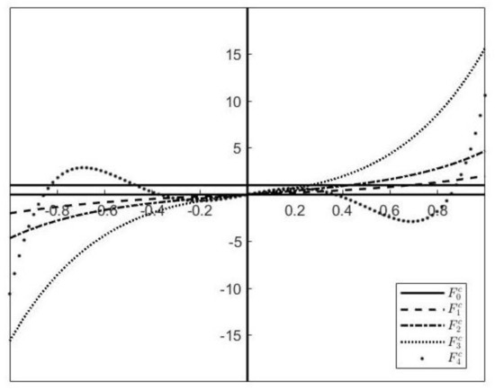
Hence, the first five odd Fibonacci-central factorial polynomials in the basis $x^{[2k+1]}$ are

$$\begin{array}{c}{\displaystyle F_0^c\left(x\right)=x^{\left[1\right]},F_1^c\left(x\right)=x^{\left[3\right]}+\frac{5}{4}{x}^{\left[1\right]},F_2^c\left(x\right)=x^{\left[5\right]}+\frac{25}{6}{x}^{\left[3\right]}+\frac{119}{48}{x}^{\left[1\right]},}\hfill \\ {\displaystyle F_3^c\left(x\right)=x^{\left[7\right]}+\frac{35}{4}{x}^{\left[5\right]}+\frac{833}{48}{x}^{\left[3\right]}+\frac{1139}{192}{x}^{\left[1\right]},}\hfill \\ {\displaystyle F_4^c\left(x\right)=x^{\left[9\right]}+15x^{\left[7\right]}+\frac{2499}{16}{x}^{\left[5\right]}+\frac{1139}{16}{x}^{\left[3\right]}-\frac{3427}{1280}{x}^{\left[1\right]}.}\hfill \end{array}$$

Figure 2 shows the plot of these polynomials.

Figure 2. Odd Fibonacci-central factorial polynomials.

The conditions

$$z_{n,0}=F_n,n=0,1,\dots ,$$

and the relation (24) allow for obtaining the polynomials written in the monomial basis.

For example, for $n=0,\dots ,5$, we have

$$\begin{array}{c}{\displaystyle F_0^c\left(x\right)=x,F_1^c\left(x\right)=x^3+x,F_2^c\left(x\right)=x^5+\frac{5}{3}{x}^3+2x,}\hfill \\ {\displaystyle F_3^c\left(x\right)=x^7+\frac{35}{3}{x}^3+3x,}\hfill \\ {\displaystyle F_4^c\left(x\right)=x^9-6x^7+\frac{273}{5}{x}^5-44x^3+5x,}\hfill \\ {\displaystyle F_5^c\left(x\right)=x^{11}-\frac{55}{3}{x}^9+231x^7-913x^5+\frac{3377}{3}{x}^3+8x.}\hfill \end{array}$$

In [27], the Fibonacci p.s. ${\left\{f_n\right\}}_{n\in \mathrm{I}\mathrm{N}}$ was analyzed. Note that the p.s. ${\left\{f_n\right\}}_{n\in \mathrm{I}\mathrm{N}}$ has an odd polynomial subsequence ${\left\{f_{2n+1}\right\}}_{n\in \mathrm{I}\mathrm{N}}$. This subsequence differs from ${\left\{F_n^c\right\}}_{n\in \mathrm{I}\mathrm{N}}$.

Example 2

(Odd Hermite-central factorial polynomial sequence). Let ${\left\{{\mathcal{H}}_n\right\}}_{n\in \mathrm{I}\mathrm{N}}$ be the well-known Hermite p.s. ([17], p. 135), ([29], p. 187). We consider the monic Hermite p.s. ${\left\{H_n\right\}}_{n\in \mathrm{I}\mathrm{N}}$ and determine the GOCPS ${\left\{d_n\right\}}_{n\in \mathrm{I}\mathrm{N}}$ such that

$$d_0^{\prime }\left(0\right)=1,d_n^{\prime }\left(0\right)=H_n^{\prime }\left(0\right)=\left\{\begin{array}{ll}{(-1)}^n{\left(\frac{3}{2}\right)}_n\hfill & \mathit{for}\mathit{even}n>0\\ 0\hfill & \mathit{for}\mathit{odd}n>0.\end{array}\right.$$

(28)

The elements of this p.s. satisfy

$$\left\{\begin{array}{c}{\delta }^2{d}_n\left(x\right)=2n\left(2n+1\right)d_{n-1}\left(x\right)\hfill \\ d_n\left(0\right)=0,d_n^{\prime }\left(0\right)=H_n^{\prime }\left(0\right),n>0.\hfill \end{array}\right.$$

We call this sequence odd Hermite-central factorial p.s., and we denote it by ${\left\{H_n^c\right\}}_{n\in \mathrm{I}\mathrm{N}}$.

From (8) and (28), for any $n\in \mathrm{I}\mathrm{N}$, we obtain ${\alpha }_{2k}$, $k=0,\dots ,n$.

For example, for $n=4$, we have

$${\alpha }_0=1,{\alpha }_2=\frac{5}{4},{\alpha }_4=\frac{23}{48},{\alpha }_6=-\frac{397}{192},{\alpha }_8=-\frac{4259}{1280}.$$

The first five odd Hermite-central factorial polynomials are

$$\begin{array}{c}{\displaystyle H_0^c\left(x\right)=x^{\left[1\right]},H_1^c\left(x\right)=x^{\left[3\right]}+\frac{5}{4}{x}^{\left[1\right]},H_2^c\left(x\right)=x^{\left[5\right]}+\frac{25}{6}{x}^{\left[3\right]}+\frac{23}{48}{x}^{\left[1\right]},}\hfill \\ {\displaystyle H_3^c\left(x\right)=x^{\left[7\right]}+\frac{35}{4}{x}^{\left[5\right]}+\frac{161}{48}{x}^{\left[3\right]}-\frac{397}{192}{x}^{\left[1\right]},}\hfill \\ {\displaystyle H_4^c\left(x\right)=x^{\left[9\right]}+15x^{\left[7\right]}+\frac{483}{40}{x}^{\left[5\right]}-\frac{397}{16}{x}^{\left[3\right]}-\frac{4259}{1280}{x}^{\left[1\right]}.}\hfill \end{array}$$

Figure 3 shows the plot of these polynomials.

Figure 3. Odd Hermite-central factorial polynomials.

By the relations (24) and (26), we obtain the polynomials written in the monomial basis.

For example, for $n=0,\dots ,5$, they are

$$\begin{array}{c}{\displaystyle H_0^c\left(x\right)=x,H_1^c\left(x\right)=x^3+x,H_2^c\left(x\right)=x^5+\frac{5}{3}{x}^3,}\hfill \\ {\displaystyle H_3^c\left(x\right)=x^7-\frac{7}{3}{x}^3-\frac{3}{2}x,}\hfill \\ {\displaystyle H_4^c\left(x\right)=x^9-6x^7+\frac{21}{5}{x}^5-14x^3,}\hfill \\ {\displaystyle H_5^c\left(x\right)=x^{11}-\frac{55}{3}{x}^9+99x^7-286x^5+297x^3+\frac{15}{4}x.}\hfill \end{array}$$

4. General Even Central Factorial Polynomial Sequences

Now, analogous with the odd case, we consider the general even central factorial polynomial sequences, that is, the polynomial sequences ${\left\{e_n\right\}}_{n\in \mathrm{I}\mathrm{N}}$ whose elements are polynomials of degree $2n$ satisfying

$$\left\{\begin{array}{c}{\delta }^2{e}_n\left(x\right)=2n\left(2n-1\right)e_{n-1}\left(x\right)\hfill \\ e_n^{\prime }\left(0\right)=0,e_0\left(x\right)=1.\hfill \end{array}\right.$$

(29)

Since all the proofs of the results concerning this type of polynomial sequences are similar to those of the odd case, we omit them.

Proposition 5.

Let ${\left\{e_n\right\}}_{n\in \mathrm{I}\mathrm{N}}$ be an even p.s. It is a GECPS, that is, it satisfies (29) if and only if a numerical sequence ${\left({\gamma }_{2n}\right)}_{n\in \mathrm{I}\mathrm{N}}$, with ${\gamma }_0\ne 0$, exists such that $\forall n\in \mathrm{I}\mathrm{N}$, $\forall x\in \mathrm{I}\mathrm{K}$,

$$e_n\left(x\right)=\sum _{k=0}^n\left(\genfrac{}{}{0pt}{}{2n}{2k}\right){\gamma }_{2(n-k)}{x}^{\left[2k\right]}.$$

Proposition 6.

Let ${\left\{e_n\right\}}_{n\in \mathrm{I}\mathrm{N}}$ be a GECPS. Then, for $j=0,\dots ,n$, we obtain

(1) 

${\displaystyle {\delta }^{2j}{e}_n\left(x\right)=\frac{\left(2n\right)!}{\left(2\right(n-j\left)\right)!}{e}_{n-j}\left(x\right)}$;

(2) 

${\displaystyle {\delta }^{2j+1}{e}_n\left(x\right)=\frac{\left(2n\right)!}{\left(2\right(n-j\left)\right)!}\delta e_{n-j}\left(x\right)}$;

(3) 

${\displaystyle {\delta }^{2j+1}{e}_n\left(0\right)=0,{\delta }^{2j}{e}_n\left(0\right)=\frac{\left(2n\right)!}{\left(2\right(n-j\left)\right)!}\delta e_{n-j}\left(0\right)}$.

Corollary 2.

For a GECPS ${\left\{e_n\right\}}_{n\in \mathrm{I}\mathrm{N}}$, $\forall n,j\in \mathrm{I}\mathrm{N}$ with $j<n$, the following identities hold:

$$\sum _{k=0}^{2j}\left(\genfrac{}{}{0pt}{}{2j}{k}\right){\left(-1\right)}^k{e}_n(x+j-k)=\frac{\left(2n\right)!}{\left(2\right(n-j\left)\right)!}{e}_{n-j}\left(x\right);$$

$$\sum _{k=0}^{2j+1}\left(\genfrac{}{}{0pt}{}{2j+1}{k}\right){\left(-1\right)}^k{e}_n\left(x+j-k+\frac{1}{2}\right)=\frac{\left(2n\right)!}{\left(2\right(n-j\left)\right)!}\delta e_{n-j}\left(x\right).$$

4.1. Matrix Form

Given a numerical sequence ${\left({\gamma }_{2k}\right)}_{k\in \mathrm{I}\mathrm{N}}$, ${\gamma }_0\ne 0$, let us consider the lower infinite triangular matrix $U_{\infty }=\left(u_{i,j}\right)$ with

$$u_{i,j}=\left\{\begin{array}{llll}& \left(\genfrac{}{}{0pt}{}{2i}{2j}\right){\gamma }_{2(i-j)},\hfill & & i\ge 0,j=0,1,\dots ,i\\ & 0\hfill & & i<j\end{array}\right.$$

The first matrix form of a GECPS is:

$${\mathbf{E}}_{\infty }={\mathbf{U}}_{\infty }{\stackrel{⌐}{\mathbf{X}}}_{\infty },\mathrm{or}\mathbf{E}=\mathbf{U}\stackrel{⌐}{\mathbf{X}},$$

(30)

where $\mathbf{U}={\mathbf{U}}_{\infty }$,

$$\stackrel{⌐}{\mathbf{X}}={\stackrel{⌐}{\mathbf{X}}}_{\infty }={\left[1,x^{\left[2\right]},\dots ,x^{\left[2\nu \right]},\dots \right]}^T,\mathbf{E}={\mathbf{E}}_{\infty }={\left[e_0\left(x\right),e_1\left(x\right),\dots ,e_{\nu }\left(x\right),\dots \right]}^T.$$

The matrix $\mathbf{U}$ can be factorized [14] as ${\displaystyle \mathbf{U}=\mathbf{G}{\mathbf{T}}_{\mathbf{f}\mathbf{l}}{\mathbf{G}}^{-\mathbf{1}}}$, where $\mathbf{G}=diag\left\{\left(2i\right)!|i\ge 0\right\}$ and ${\mathbf{T}}_{\mathbf{\gamma }}$ is a lower triangular Toepliz matrix with elements ${\displaystyle t_{i,j}^{\gamma }=\frac{{\gamma }_{2(i-j)}}{\left(2\right(i-j\left)\right)!}}$.

$\mathbf{U}$ is invertible and ${\displaystyle {\mathbf{U}}^{-\mathbf{1}}=\mathbf{G}{\mathbf{T}}_{\mathbf{1}}{\mathbf{G}}^{-\mathbf{1}}}$, where ${\mathbf{T}}_{\mathbf{1}}$ is a lower triangular Toepliz matrix with elements ${\displaystyle t_{i,j}^{\beta }=\frac{{\zeta }_{2(i-j)}}{\left(2\right(i-j\left)\right)!}}$, ${\left({\zeta }_{2k}\right)}_{k\in \mathrm{I}\mathrm{N}}$ being the numerical sequence defined by

$$\sum _{j=0}^i\frac{{\gamma }_{2j}{\zeta }_{2(i-j)}}{\left(2j\right)!\left(2\right(i-j\left)\right)!}={\delta }_{i0},i\ge 0.$$

(31)

Let ${\mathbf{U}}_{\mathbf{n}}$ be the principal submatrix of order $n+1$ of $\mathbf{U}$ and let ${\stackrel{⌐}{\mathbf{X}}}_{\mathbf{n}}$ and ${\mathbf{E}}_{\mathbf{n}}$ be the principal subvectors with $n+1$ components of ${\stackrel{⌐}{\mathbf{X}}}_{\infty }$ and ${\mathbf{E}}_{\infty }$, respectively. Then, from (30),

$${\mathbf{E}}_{\mathbf{n}}={\mathbf{U}}_{\mathbf{n}}{\stackrel{⌐}{\mathbf{X}}}_{\mathbf{n}}.$$

(32)

4.2. Conjugate Even Polynomials

Let ${\left({\gamma }_{2k}\right)}_{k\in \mathrm{I}\mathrm{N}}$, ${\gamma }_0\ne 0$, be a given numerical sequence and ${\left({\zeta }_{2k}\right)}_{k\in \mathrm{I}\mathrm{N}}$ the related sequence defined as in (31). For any $k\in \mathrm{I}\mathrm{N}$, we can consider the polynomial

$${\widehat{e}}_k\left(x\right)=\sum _{j=0}^k\left(\genfrac{}{}{0pt}{}{2k}{2j}\right){\zeta }_{2j}{x}^{\left[2\right(k-j\left)\right]}=\sum _{j=0}^k\left(\genfrac{}{}{0pt}{}{2k}{2j}\right){\zeta }_{2(k-j)}{x}^{\left[2j\right]}.$$

(33)

From this identity and Proposition 5, the sequence ${\left\{{\widehat{e}}_k\right\}}_{k\in \mathrm{I}\mathrm{N}}$ is a GECPS. We call the sequences ${\left\{e_k\right\}}_{k\in \mathrm{I}\mathrm{N}}$, ${\left\{{\widehat{e}}_k\right\}}_{k\in \mathrm{I}\mathrm{N}}$ conjugate even central polynomial sequences.

By setting $\mathbf{B}=\left(b_{i,j}\right)$, with

$$b_{i,j}=\left\{\begin{array}{llll}& \left(\genfrac{}{}{0pt}{}{2i}{2j}\right){\zeta }_{2(i-j)},\hfill & & i\ge 0,j=0,1,\dots ,i\\ & 0\hfill & & i<j,\end{array}\right.$$

and $\widehat{\mathbf{E}}={\widehat{\mathbf{E}}}_{\infty }=\left[{\widehat{e}}_0\left(x\right),{\widehat{e}}_1\left(x\right),\dots ,{\widehat{e}}_{\nu }\left(x\right),\dots \right]$, from (33), we have

$$\widehat{\mathbf{E}}=\mathbf{B}\stackrel{}{\mathbf{X}}\mathrm{and}{\widehat{\mathbf{E}}}_{\mathbf{n}}={\mathbf{B}}_{\mathbf{n}}{\stackrel{}{\mathbf{X}}}_{\mathbf{n}},\forall n\in \mathrm{I}\mathrm{N}.$$

Moreover,

$$\left\{\begin{array}{l}\hfill \mathbf{E}={\mathbf{U}}^{\mathbf{2}}\widehat{\mathbf{E}}\\ \hfill \widehat{\mathbf{E}}={\mathbf{B}}^{\mathbf{2}}\mathbf{E}\end{array}\right.\mathrm{and}\left\{\begin{array}{l}\hfill {\mathbf{E}}_{\mathbf{n}}={\mathbf{U}}_{\mathbf{n}}^{\mathbf{2}}{\widehat{\mathbf{E}}}_{\mathbf{n}}\\ \hfill {\widehat{\mathbf{E}}}_{\mathbf{n}}={\mathbf{B}}_{\mathbf{n}}^{\mathbf{2}}{\mathbf{E}}_{\mathbf{n}},\end{array}\right.\forall n\in \mathrm{I}\mathrm{N},$$

where ${\mathbf{U}}^{\mathbf{2}}=\mathbf{U}\mathbf{U}=\left({\mathbf{u}}_{\mathbf{i},\mathbf{j}}^{*}\right)$, and ${\mathbf{B}}^{\mathbf{2}}=\mathbf{B}\mathbf{B}=\left(b_{i,j}^{*}\right)$. Finally, $\forall n\in \mathrm{I}\mathrm{N}$,

$$e_n\left(x\right)=\sum _{j=0}^n{u}_{n,j}^{*}{\widehat{e}}_j\left(x\right),{\widehat{e}}_n\left(x\right)=\sum _{j=0}^n{b}_{n,j}^{*}{e}_j\left(x\right).$$

4.3. Recurrence Relation and Related Determinant Form

From the identity (32), we have

$${\stackrel{⌐}{\mathbf{X}}}_{\mathbf{n}}={\mathbf{U}}_{\mathbf{n}}^{-\mathbf{1}}{\mathbf{E}}_{\mathbf{n}},$$

and, for $k=0,\dots ,n$,

$$x^{\left[2k\right]}=\sum _{j=0}^k\left(\genfrac{}{}{0pt}{}{2k}{2j}\right){\zeta }_{2(k-j)}{e}_j\left(x\right).$$

Theorem 7

(Recurrence relation). Let ${\left\{e_n\right\}}_{n\in \mathrm{I}\mathrm{N}}$ be an even p.s. It is a GECPS if and only if there exist numerical sequences ${\left({\gamma }_{2k}\right)}_{k\in \mathrm{I}\mathrm{N}}$, ${\left({\zeta }_{2k}\right)}_{k\in \mathrm{I}\mathrm{N}}$, with ${\gamma }_0\ne 0$, ${\zeta }_0\ne 0$, satisfying the relation (31), such that, $\forall k\ge 1$,

$$e_k\left(x\right)=\frac{1}{{\zeta }_0}\left[x^{\left[2k\right]}-\sum _{j=0}^{k-1}\left(\genfrac{}{}{0pt}{}{2k}{2j}\right){\zeta }_{2(k-j)}{e}_j\left(x\right)\right].$$

Remark 10.

For the elements of the conjugate sequence ${\left\{{\widehat{e}}_n\right\}}_{n\in \mathrm{I}\mathrm{N}}$, the first recurrence relation is

$${\widehat{e}}_n\left(x\right)=\frac{1}{{\gamma }_0}\left[x^{\left[2k\right]}-\sum _{j=0}^{k-1}\left(\genfrac{}{}{0pt}{}{2k}{2j}\right){\gamma }_{2(k-j)}{\widehat{e}}_j\left(x\right)\right].$$

Theorem 8

(Determinant form). Let ${\left\{e_n\right\}}_{n\in \mathrm{I}\mathrm{N}}$ be a GECPS as in Theorem 7. Then,

$$\begin{array}{c}{\displaystyle e_0\left(x\right)=\frac{1}{{\zeta }_0},}\hfill \\ {\displaystyle e_k\left(x\right)=\frac{{\left(-1\right)}^k}{{\zeta }_0^{k+1}}\left|\begin{array}{cccccc}1& x^{\left[2\right]}& x^{\left[4\right]}& \dots & x^{[2k-2]}& x^{\left[2k\right]}\\ {\zeta }_0& {\zeta }_2& {\zeta }_4& \dots & {\zeta }_{2(k-1)}& {\zeta }_{2k}\\ 0& {\zeta }_0& \left(\genfrac{}{}{0pt}{}{4}{2}\right){\zeta }_2& \dots & \left(\genfrac{}{}{0pt}{}{2k-2}{2}\right){\zeta }_{2(k-2)}& \left(\genfrac{}{}{0pt}{}{2k}{2}\right){\zeta }_{2(k-1)}\\ ⋮& \ddots & \ddots & & ⋮& ⋮\\ ⋮& & \ddots & & ⋮& ⋮\\ ⋮& & & & ⋮& ⋮\\ 0& \dots & \dots & & {\zeta }_0& \left(\genfrac{}{}{0pt}{}{2k}{2(k-1)}\right){\zeta }_2\end{array}\right|,k\ge 1.}\hfill \end{array}$$

The elements of the conjugate sequence ${\left\{{\widehat{e}}_n\right\}}_{n\in \mathrm{I}\mathrm{N}}$ are such that

$$\begin{array}{c}{\displaystyle {\widehat{e}}_0\left(x\right)=\frac{1}{{\gamma }_0},}\hfill \\ {\displaystyle {\widehat{e}}_k\left(x\right)=\frac{{\left(-1\right)}^k}{{\gamma }_0^{k+1}}\left|\begin{array}{cccccc}1& x^{\left[2\right]}& x^{\left[4\right]}& \dots & x^{[2k-2]}& x^{\left[2k\right]}\\ {\gamma }_0& {\gamma }_2& {\gamma }_4& \dots & {\gamma }_{2(k-1)}& {\gamma }_{2k}\\ 0& {\gamma }_0& \left(\genfrac{}{}{0pt}{}{4}{2}\right){\gamma }_2& \dots & \left(\genfrac{}{}{0pt}{}{2k-2}{2}\right){\gamma }_{2(k-2)}& \left(\genfrac{}{}{0pt}{}{2k}{2}\right){\gamma }_{2(k-1)}\\ ⋮& \ddots & \ddots & & ⋮& ⋮\\ ⋮& & \ddots & & ⋮& ⋮\\ ⋮& & & & ⋮& ⋮\\ 0& \dots & \dots & & {\gamma }_0& \left(\genfrac{}{}{0pt}{}{2k}{2(k-1)}\right){\gamma }_2\end{array}\right|,k\ge 1.}\hfill \end{array}$$

4.4. The Linear Space $\widetilde{GECPS}$

Definition 4.

Let ${\left\{e_k\right\}}_{k\in \mathrm{I}\mathrm{N}}$ and ${\left\{e_k^{*}\right\}}_{k\in \mathrm{I}\mathrm{N}}$ be the general central polynomial sequences related to the numerical sequences ${\left({\eta }_{2k}\right)}_{k\in \mathrm{I}\mathrm{N}}$ and ${\left({\upsilon }_{2k}\right)}_{k\in \mathrm{I}\mathrm{N}}$, respectively. That is, $\forall k\in \mathrm{I}\mathrm{N}$,

$$e_k\left(x\right)=\sum _{j=0}^k\left(\genfrac{}{}{0pt}{}{2k}{2j}\right){\eta }_{2(k-j)}{x}^{\left[2j\right]},e_k^{*}\left(x\right)=\sum _{j=0}^k\left(\genfrac{}{}{0pt}{}{2k}{2j}\right){\upsilon }_{2(k-j)}{x}^{\left[2j\right]}.$$

For all $k\in \mathrm{I}\mathrm{N}$, the umbral composition of $e_k\left(x\right)$ and $e_k^{*}\left(x\right)$ is

$$w_k\left(x\right):=\left(e_k\circ e_k^{*}\right)\left(x\right)=\sum _{j=0}^k\left(\genfrac{}{}{0pt}{}{2k}{2j}\right){\eta }_{2(k-j)}{e}_j^{*}\left(x\right).$$

It is easy to verify that

• ${\left\{w_k\right\}}_{k\in \mathrm{I}\mathrm{N}}={\left\{e_k\circ e_k^{*}\right\}}_{k\in \mathrm{I}\mathrm{N}}$ is a GECPS;
• $\forall k\in \mathrm{I}\mathrm{N},\left(e_k\circ {\widehat{e}}_k\right)\left(x\right)=x^{\left[2k\right]}$.

Moreover, if "+" and "·" are, respectively, the usual sum and product for a scalar on the set of even polynomial sequences, then $\widetilde{GECPS}=\left(GECPS,+,·,\circ \right)$ is an algebra.

4.5. Generating Function

Let $G\left(t\right)$ be the power series

$$G\left(t\right)=t+\sum _{n=1}^{\infty }{(-1)}^n\left(\prod _{k=1}^n\frac{{(2k-1)}^2}{4}\right)\frac{t^{2n+1}}{(2n+1)!}.$$

Then, taking into account that

$$coshx\left(xG\left(t\right)\right)=\sum _{k=0}^{\infty }\frac{{\left(xG\left(t\right)\right)}^{2k}}{\left(2k\right)!},$$

we have

$$cosh\left(xG\left(t\right)\right)=\sum _{\nu =0}^{\infty }{x}^{\left[2\nu \right]}\frac{t^{2\nu }}{\left(2\nu \right)!}.$$

Hence, the function

$$g\left(x,t\right)=cosh\left(xG\left(t\right)\right)$$

is the generating function of even central factorial polynomials $x^{\left[2\nu \right]}$.

Theorem 9.

The generating function of a GECPS related to the numerical sequence ${\left({\gamma }_{2k}\right)}_{k\in \mathrm{I}\mathrm{N}}$ is

$$F\left(x,t\right)=l\left(t\right)g(x,t),$$

with

$$l\left(t\right)=\sum _{k=0}^{\infty }{\gamma }_{2k}\frac{t^{2k}}{\left(2k\right)!}.$$

4.6. Connection to the Basic Monomials $x^{2i}$

From (20),

$$x^{\left[2k\right]}=\sum _{i=0}^{k}t\left(2k,i\right)x^{2i}.$$

If ${\Omega }^{\mathbf{t}}={\left({\omega }_{i,j}^t\right)}_{i,j\in \mathrm{I}\mathrm{N}}$, with

$${\omega }_{i,j}^t=\left\{\begin{array}{cc}t\left(2i,j\right)\hfill & i\ge j\hfill \\ 0\hfill & i<j,\hfill \end{array}\right.$$

then

$$\stackrel{⌐}{\mathbf{X}}={\Omega }^{\mathbf{t}}\tilde{\mathbf{X}},$$

(34)

where $\tilde{\mathbf{X}}={\left[1,x^2,\dots ,x^{2\nu },\dots \right]}^T$.

Let ${\left\{e_k\right\}}_{k\in \mathrm{I}\mathrm{N}}$ be the GECPS related to the numerical sequence ${\left({\gamma }_{2k}\right)}_{k\in \mathrm{I}\mathrm{N}}$. Let $\mathbf{E}$ be as in (30). Then, by substituting (34) in (30), we obtain

$$\mathbf{E}=\left(\mathbf{U}{\mathbf{W}}^{\mathbf{t}}\right)\tilde{\mathbf{X}},$$

that is,

$$e_n\left(x\right)=\sum _{j=0}^i{s}_{n,j}{x}^{2j}\mathrm{with}{s}_{n,j}=\sum _{k=0}^n{u}_{n,k}{w}_{k,j}^t.$$

(35)

Remark 11.

The following identity holds

$$e_n\left(0\right)=s_{n,0},n\ge 0.$$

(36)

Theorem 10.

Let ${\left(s_{n,0}\right)}_{n\in \mathrm{I}\mathrm{N}}$ be an assigned numerical sequence. Then, the sequence ${\left\{e_n\right\}}_{n\in \mathrm{I}\mathrm{N}}$ with $e_n$ as (35) is a GECPS if and only if the coefficients, $s_{n,j},j=0,1,\dots ,n$, are the solution of the system

$$\sum _{i=j+1}^n\left(\genfrac{}{}{0pt}{}{2i}{2j}\right)s_{n,i}=n(2n-1)s_{n-1,j},j=0,\dots ,n-1.$$

Remark 12.

From backward substitutions,

$$s_{n,j}=\frac{n(2n-1)}{j(2j-1)}{s}_{n-1,j-1}-\frac{1}{j(2j-1)}\sum _{i=j+1}^n\left(\genfrac{}{}{0pt}{}{2i}{2j-2}\right)s_{n,i},j=n-1,\dots ,1.$$

(37)

4.7. Examples

Now, we give some examples of general even central factorial polynomial sequences.

Firstly, from Proposition 5, if ${\left({\gamma }_{2k}\right)}_{k\in \mathrm{I}\mathrm{N}}$, ${\gamma }_0\ne 0$, is an assigned numerical sequence, we determine the related GECPS, that is, the p.s. ${\left\{e_n\right\}}_{n\in \mathrm{I}\mathrm{N}}$ such that

$$e_n\left(x\right)=\sum _{k=0}^n\left(\genfrac{}{}{0pt}{}{2n}{2k}\right){\gamma }_{2(n-k)}{x}^{\left[2k\right]},\forall n\in \mathrm{I}\mathrm{N},\forall x\in \mathrm{I}\mathrm{K}.$$

Then, we write $e_n$ in the monomial basis $x^{2i}$, according to (35). It satisfies (36).

Example 3

(Even Fibonacci-central factorial p.s.). We will determine the GECPS ${\left\{e_n\right\}}_{n\in \mathrm{I}\mathrm{N}}$ such that

$$e_n\left(0\right)=F_n,\forall n\in \mathrm{I}\mathrm{N},$$

(38)

where ${\left(F_n\right)}_{n\in \mathrm{I}\mathrm{N}}$ is the Fibonacci numerical sequence.

The elements of this p.s. satisfy

$$\left\{\begin{array}{c}{\delta }^2{e}_n\left(x\right)=2n\left(2n-1\right)e_{n-1}\left(x\right)\hfill \\ e_n^{\prime }\left(0\right)=0,e_n\left(0\right)=F_n.\hfill \end{array}\right.$$

In this case, we call${\left\{e_n\right\}}_{n\in \mathrm{I}\mathrm{N}}$ even Fibonacci-central factorial p.s. and we denote it by ${\left\{F_n^e\right\}}_{n\in \mathrm{I}\mathrm{N}}$.

For every $n\in \mathrm{I}\mathrm{N}$, the conditions (38) give the coefficients ${\gamma }_{2k}=F_k$, $k=0,\dots ,n$.

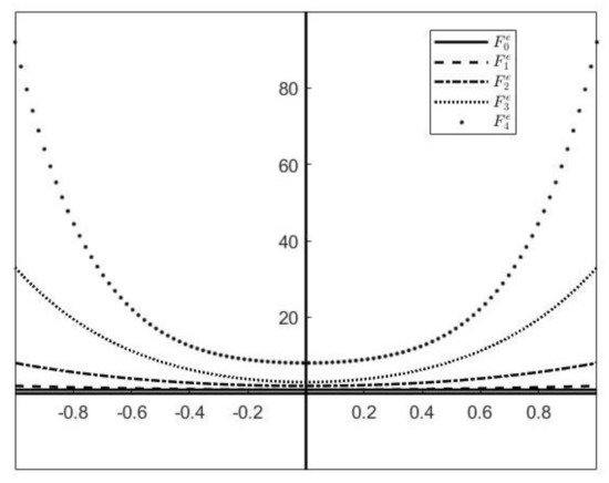
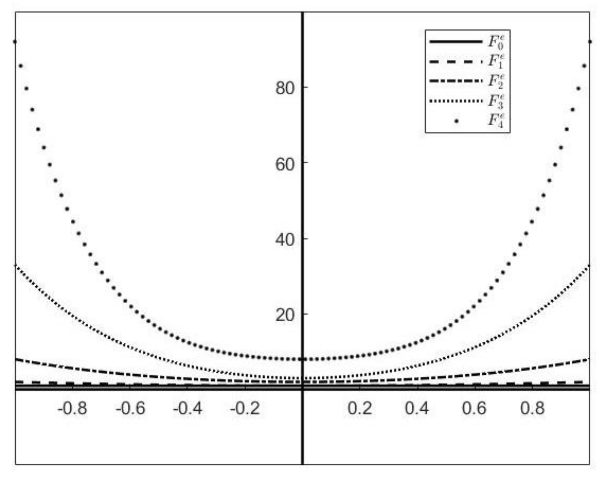
For example, for $n=0,\dots ,4$, we obtain the polynomials

$$\begin{array}{c}{\displaystyle F_0^e\left(x\right)=x^{\left[0\right]},F_1^e\left(x\right)=x^{\left[2\right]}+x^{\left[0\right]},F_2^e\left(x\right)=x^{\left[4\right]}+6x^{\left[2\right]}+2x^{\left[0\right]},}\hfill \\ {\displaystyle F_3^e\left(x\right)=x^{\left[6\right]}+15x^{\left[4\right]}+30x^{\left[2\right]}+3x^{\left[0\right]},}\hfill \\ {\displaystyle F_4^e\left(x\right)=x^{\left[8\right]}+28x^{\left[6\right]}+140x^{\left[4\right]}+84x^{\left[2\right]}+5x^{\left[0\right]}.}\hfill \end{array}$$

Figure 4 shows the plot of these polynomials.

Figure 4. Even Fibonacci-central factorial polynomials.

From the relations (36) and the conditions

$$F_n^e\left(0\right)=s_{n,0}=F_n,n=0,1,\dots ,$$

we obtain the polynomials $F_n^e$ written into the even monomial basis.

For example, for $n=5$, we have

$$\begin{array}{c}{F}_0^e\left(x\right)=1,e_1\left(x\right)=x^2+1,F_2^e\left(x\right)=x^4+5x^2+2,\hfill \\ F_3^e\left(x\right)=x^6+10x^4+19x^2+3,\hfill \\ F_4^e\left(x\right)=x^8+14x^6+49x^4+20x^2+5,\hfill \\ F_5^e\left(x\right)=x^{10}+15x^8+63x^6-85x^4+231x^2+8.\hfill \end{array}$$

Example 4

(Even Hermite-central factorial p.s.). Now, we determine the GECPS ${\left\{e_n\right\}}_{n\in \mathrm{I}\mathrm{N}}$ such that

$$e_0\left(0\right)=1,e_n\left(0\right)=H_n\left(0\right)=\left\{\begin{array}{ll}{(-1)}^n{\left(\frac{1}{2}\right)}_n\hfill & \mathit{for}\mathit{even}n>0\\ 0\hfill & \mathit{for}\mathit{odd}n>0,\end{array}\right.$$

(39)

${\left\{H_n\right\}}_{n\in \mathrm{I}\mathrm{N}}$ being the monic Hermite p.s. ([17], p. 135).

The elements of ${\left\{e_n\right\}}_{n\in \mathrm{I}\mathrm{N}}$ satisfy

$$\left\{\begin{array}{c}{\delta }^2{e}_n\left(x\right)=2n\left(2n+1\right)e_{n-1}\left(x\right)\hfill \\ e_n\left(0\right)=0,e_n\left(0\right)=H_n\left(0\right).\hfill \end{array}\right.$$

We call${\left\{e_n\right\}}_{n\in \mathrm{I}\mathrm{N}}$ even Hermite-central factorial p.s., and we denote it by ${\left\{H_n^e\right\}}_{n\in \mathrm{I}\mathrm{N}}$.

From (39), for any $n\in \mathrm{I}\mathrm{N}$, we obtain ${\gamma }_{2n}=H_n\left(0\right)$.

The first five odd Hermite-central factorial polynomials are

$$\begin{array}{c}{\displaystyle H_0^e\left(x\right)=x^{\left[0\right]},H_1^e\left(x\right)=x^{\left[2\right]},H_2^e\left(x\right)=x^{\left[4\right]}-\frac{1}{2}{x}^{\left[0\right]},}\hfill \\ {\displaystyle H_3^e\left(x\right)=x^{\left[6\right]}-\frac{15}{2}{x}^{\left[2\right]},}\hfill \\ {\displaystyle H_4^e\left(x\right)=x^{\left[8\right]}-35x^{\left[4\right]}+\frac{3}{4}{x}^{\left[0\right]}.}\hfill \end{array}$$

Figure 5 shows the plot of these polynomials.

Figure 5. Even Hermite-central factorial polynomials.

Written in the monomial basis, they become

$$\begin{array}{c}{\displaystyle H_0^e\left(x\right)=1,H_1^e\left(x\right)=x^2,H_2^e\left(x\right)=x^4-x^2-\frac{1}{2},}\hfill \\ {\displaystyle H_3^e\left(x\right)=x^6-5x^4-\frac{7}{2}{x}^2,}\hfill \\ {\displaystyle H_4^e\left(x\right)=x^8-14x^6+14x^4-x^2+\frac{3}{4}.}\hfill \end{array}$$

5. Conclusions

In this paper, we considered the operator ${\delta }^2(·)$, where $\delta (·)$ is the known central difference operator. The general polynomial solutions of the following two problems

$$\left\{\begin{array}{c}{\delta }^2{d}_n\left(x\right)=2n\left(2n+1\right)d_{n-1}\left(x\right),n\ge 1\hfill \\ d_n\left(0\right)=0,deg\left(d_n\right)=2n+1,n\ge 0\hfill \end{array}\right.$$

and

$$\left\{\begin{array}{c}{\delta }^2{e}_n\left(x\right)=2n\left(2n-1\right)e_{n-1}\left(x\right),n\ge 1\hfill \\ e_n^{\prime }\left(0\right)=0,deg\left(e_n\right)=2n,n\ge 0,\hfill \end{array}\right.$$

have been studied.

These solutions were called general odd (respectively, even) central factorial polynomial sequences and denoted by GOCPS and GECPS, respectively. Each polynomial has been written both in the basis $x^{[2i+1]}$ (resp. $x^{\left[2i\right]}$) and in the basis $x^{2i+1}$ (resp. $x^{2i}$). The matrix and determinant forms and a recurrence formula have been provided. The generating functions for the two kinds of polynomial sequences have also been obtained. An interesting property of biorthogonality has been demonstrated. Finally, two new general odd (even) central factorial p.s., called Fibonacci central factorial and Hermite central factorial p.s., have been given.

Future research in this direction, both theoretical and computational, is possible. For example, the general operator of the type $Qy={\sum }_{k=1}^{\infty }{c}_k{y}^{\left(2k\right)}$, $c_1\ne 0$ can be considered and the associated odd and even polynomial sequences can be determined. Computational applications, such as linear interpolation, quadrature formulas and approximation functions, can be studied. Boundary and initial value problems for difference equations can also be considered.

References

- Weierstrass, K. Über die analytische Darstellbarkeit sogenannter willkürlicher Funktionen einer reellen Veränderlichen. Sitzungsberichte der Königlich Preussischen Akademie der Wissenschaften zu Berlin 1885, 633–639, 789–805. [Google Scholar]
- Chen, X.; Tan, J.; Liu, Z.; Xie, J. Approximation of functions by a new family of generalized Bernstein operators. J. Math. Anal. Appl. 2017, 450, 244–261. [Google Scholar] [CrossRef] [Scilit]
- Srivastava, H.M.; Ansari, K.J.; Özger, F.; Özger, Z.Ö. A link between approximation theory and summability methods via four-dimensional infinite matrices. Mathematics 2021, 9, 1895. [Google Scholar] [CrossRef] [Scilit]
- Steffens, K. The History of Approximation Theory: From Euler to BErnstein; Springer Science Business Media: Berlin, Germany, 2007. [Google Scholar]
- Szegô, G. Orthogonal Polynomials; American Mathematical Society: Providence, RI, USA, 1939; Volume 23. [Google Scholar]
- Whittaker, J.M. Interpolatory Function Theory; The University Press: Cambridge/London, UK, 1935; Volume 33. [Google Scholar]
- Costabile, F.A.; Gualtieri, M.I.; Napoli, A. Recurrence relations and determinant forms for general polynomial sequences. Application to Genocchi polynomials. Integral Transform. Spec. Funct. 2019, 30, 112–127. [Google Scholar] [CrossRef] [Scilit]
- Costabile, F.A.; Longo, E. A determinantal approach to Appell polynomials. J. Comput. Appl. Math. 2010, 234, 1528–1542. [Google Scholar] [CrossRef] [Scilit]
- Costabile, F.A.; Longo, E. The Appell interpolation problem. J. Comput. Appl. Math. 2011, 236, 1024–1032. [Google Scholar] [CrossRef] [Scilit]
- Costabile, F.A.; Longo, E. δh-Appell sequences and related interpolation problem. Numer. Algorithms 2013, 63, 165–186. [Google Scholar] [CrossRef] [Scilit]
- Costabile, F.A.; Longo, E. An algebraic approach to Sheffer polynomial sequences. Integral Transform. Spec. Funct. 2014, 25, 295–311. [Google Scholar] [CrossRef] [Scilit]
- Costabile, F.A.; Longo, E. An algebraic exposition of umbral calculus with application to general linear interpolation problem: A survey. Publ. L’Inst. Math. 2014, 96, 67–83. [Google Scholar] [CrossRef] [Scilit]
- Lidstone, G.J. Notes on the Extension of Aitken’s Theorem (for Polynomial Interpolation) to the Everett Types. Proc. Edinb. Math. Soc. 1930, 2, 16–19. [Google Scholar] [CrossRef] [Scilit]
- Costabile, F.A.; Gualtieri, M.I.; Napoli, A. Odd and even Lidstone-type polynomial sequences. Part 1: Basic topics. Adv. Differ. Equation 2018, 2018, 299. [Google Scholar] [CrossRef] [Scilit]
- Costabile, F.A.; Gualtieri, M.I.; Napoli, A. Odd and even Lidstone-type polynomial sequences. Part 2: Applications. Calcolo 2020, 57, 1–35. [Google Scholar] [CrossRef] [Scilit]
- Steffensen, J.F. Interpolation; Courier Corporation: Chelmsford, MA, USA, 2006. [Google Scholar]
- Costabile, F.A. Modern Umbral Calculus. An Elementary Introduction with Applications to Linear Interpolation and Operator Approximation Theory; Walter de Gruyter GmbH & Co. KG: Berlin, Germany, 2019; Volume 72. [Google Scholar]
- Riordan, J. Combinatorial Identities; Wiley: Hoboken, NJ, USA, 1968. [Google Scholar]
- Roman, S. The Umbral Calculus; Academic Press: New York, NY, USA, 1984. [Google Scholar]
- Roman, S.M.; Rota, G.C. The umbral calculus. Adv. Math. 1978, 27, 95–188. [Google Scholar] [CrossRef] [Scilit]
- Butzer, P.L.; Schmidt, K.; Stark, E.L.; Vogt, L. Central factorial numbers; their main properties and some applications. Numer. Funct. Anal. Optim. 1989, 10, 419–488. [Google Scholar] [CrossRef] [Scilit]
- Butzer, P.L.; Schmidt, M. Central factorial numbers and their role in finite difference calculus and approximation. Colloq. Math. Soc. 1990, 58, 127–150. [Google Scholar]
- Gelineau, Y.; Zeng, J. Combinatorial interpretations of the Jacobi-Stirling numbers. arXiv 2009, arXiv:0905.2899. [Google Scholar] [CrossRef] [Scilit]
- Kang, J.Y.; Ryoo, C.S. A research on a certain family of numbers and polynomials related to Stirling numbers, central factorial numbers, and Euler numbers. J. Appl. Math. 2013, 2013, 158130. [Google Scholar] [CrossRef] [Scilit]
- Merca, M. Connections between central factorial numbers and Bernoulli polynomials. Period. Math. Hungar. 2016, 73, 259–264. [Google Scholar] [CrossRef] [Scilit]
- Zaid, Y.H.; Shiha, F.A.; El-Desouky, B.S. Generalized central factorial numbers with odd arguments. Open J. Model. Simul. 2020, 8, 61–72. [Google Scholar] [CrossRef]
- Costabile, F.A.; Gualtieri, M.I.; Napoli, A. Polynomial sequences: Elementary basic methods and application hints. A survey. Rev. Real Acad. Cienc. Exactas, FíSicas Nat. Ser. MatemáTicas 2019, 113, 3829–3862. [Google Scholar] [CrossRef] [Scilit]
- Vorobiev, N.N. Fibonacci Numbers; Springer Science & Business Media: Berlin, Germany, 2002. [Google Scholar]
- Rainville, E.D. Special Functions; Chelsea Publishing Company: New York, NY, USA, 1960; Volume 5. [Google Scholar]
Publisher’s Note: MDPI stays neutral with regard to jurisdictional claims in published maps and institutional affiliations. |
© 2022 by the authors. Licensee MDPI, Basel, Switzerland. This article is an open access article distributed under the terms and conditions of the Creative Commons Attribution (CC BY) license (https://creativecommons.org/licenses/by/4.0/).