Mean-Square Strong Stability and Stabilization of Discrete-Time Markov Jump Systems with Multiplicative Noises

Abstract

In this paper, the mean-square strong stability and stabilization of discrete-time Markov jump systems are studied. Firstly, the definition of mean-square strong stability is given, and the necessary and sufficient conditions for mean-square strong stability are derived. Secondly, several necessary and sufficient conditions for mean-square strong stabilization via a state feedback controller and an output feedback controller are obtained. Furthermore, explicit expressions for the state feedback controller and static output feedback controller are obtained. Finally, two examples are given to illustrate the validity of the above results.

1. Introduction

As one of the most basic dynamic models, the Markov jump system has been studied extensively. This is mainly because these system models have many applications in engineering and finance, such as nuclear fission and population models, immunology, and portfolio optimization [1,2,3]. Therefore, research on the stability and control of these systems has gradually become a hot topic in the field of control theory and application. For example, the authors in [4,5] discussed the continuous-time Markov jump system and studied its stability and stabilization. In [6], the adaptive tracking problem of stochastic nonlinear systems with Markov switching was studied. Robust $H_{\infty }$ control for uncertain discrete stochastic bilinear systems was studied in [7]. Output tracking control problems for a class of switched linear systems were studied in [8]. In addition, the authors in [9,10] discussed the stability analysis of different Markovian jump systems, as well as some applications.

In practical engineering applications, the system is often required to have good transient performance and stability performance, which to a large extent limits the traditional meaning of the mean-square stability in engineering applications. For example, excessive equipment voltage in the power system may lead to irreversible damage to the power equipment [11]. A large overshoot indicates that the state of the system fluctuates greatly within a short period of time, indicating that the transient energy of the system may be too large and causing serious consequences. Therefore, it is of great significance to study how to restrain the overshoot response that a large overshoot indicates. Many scholars have made considerable achievements in this field. For instance, the authors in [12] presented the specification of optimal overshoot controllers when the controller order is fixed and the closed-loop system poles are at a fixed location. In [13,14,15], the notion of strong stability was introduced to restrain the overshoot response in different systems. The authors in [16] studied the problem of overcoming overshoot performance limitations for a class of minimum-phase linear time-invariant systems with relative degree one. The authors in [17] proposed a secondary frequency control approach to solve the problem of overshoot in the power-imbalance allocation control of power systems. Moreover, in recent years, the strong stability of systems with double and multiple delays has been studied [18,19]. Other relevant studies can be referred to [20,21]. However, there are few studies involving restricting the overshoot in discrete-time Markov jump systems.

Research on the sufficient and necessary conditions for the mean-square stability of the discrete-time Markov jump system can be traced back to 1993. The sufficient and necessary conditions for the mean-square stability of the discrete-time Markov jump systems were given, and these conditions could be transformed into a form suitable for solving for the existence of a unique solution of a set of Lyapunov equations [22]. In [23], the $l^2$ stability of discrete-time Markov jump systems was studied, and the sufficient and necessary conditions for $l^2$ stability were given, which is essentially equivalent to the mean-square stability. In [24], the classical theories of Markov jump systems were systematically introduced and studied. However, in the classical study of mean-square stability, the stability and stability problems are usually transformed into the form for solving a set of linear matrix inequalities (LMI), which can be solved using the LMI toolbox. Although this method is effective, it cannot give the explicit solution for the controller.

The key difficulty in solving these problems that have not been previously solved is twofold. On the one hand, the controller should be designed so that the system produces as little overshoot as possible under the premise of stability. On the other hand, there is the problem of finding the analytical solution of the controller without using the LMI toolbox. To sum up, we introduce the definition of mean-square strong stability in the discrete-time Markov jump system for the first time. As a stronger definition, mean-square strong stability can suppress the generation of overshoot well in the stochastic system and can improve the transient performance of the system. The main contributions of this paper are as follows. (i) The concept of mean-square strong stability of the discrete-time Markov jump system with multiplicative noise is proposed, and the necessary and sufficient condition for mean-square strong stability of the system is obtained. (ii) The design of a state feedback controller and static output feedback controller for the discrete-time Markov jump system is studied. Furthermore, two necessary and sufficient conditions are obtained to solve the controller. Finally, the analytical expressions of state feedback controllers and static output feedback controllers are given, using Finsler’s theorem.

The specific notations used in this paper are as follows. $R^n$: the set of all real n-dimensional vectors. $\mathcal{C}$: the set of all complex numbers. ${\mathbf{N}}_0$: ${\mathbf{N}}_0=\mathbf{N}\cup \left\{0\right\}$. $R^{n\times m}$: the set of all $n\times m$ matrices. $A^T$: the transpose of A. $\lambda \left(A\right)$: the eigenvalue of A. $\parallel x\parallel$: the Euclidean norm of x, where x is a vector. $\parallel A\parallel$: the Euclidean norm of A, where A is a matrix. $E(·)$: the operation of taking the mathematical expectation. A>0 $(A\ge 0,A<0,A\le 0)$: A is a real symmetric positive definite (positive semi-definite, negative definite, negative semi-definite, respectively) matrix. $B^{\perp }$: the left annihilator of B is a matrix of maximal rank such that $B^{\perp }B=0$.

2. Mean-Square Strong Stability Analysis

As important random switching systems, Markov jump systems are widely used in system control, including in motor systems, image enhancement, medical study, etc. [25,26]. In this paper, we consider the following discrete-time Markov jump systems:

$$\left\{\begin{array}{c}\begin{array}{cc}\hfill x(k+1)& =A_0\left(r_k\right)x\left(k\right)+B_0\left(r_k\right)u\left(k\right)+\sum _{n=1}^N(A_n\left(r_k\right)x\left(k\right)+B_n\left(r_k\right)u\left(k\right)){\omega }_n\left(k\right)\hfill \end{array}\hfill \\ y\left(k\right)=C\left(r_k\right)x\left(k\right),\hfill \end{array}\right.$$

(1)

where $x\left(k\right)$ is a n-dimensional state vector, $u\left(k\right)$ is the control input, and $y\left(k\right)$ is the output. The definition of multiplicative noises is that ${\omega }_n\left(k\right)\in R,n=1,2,\cdots$, N are sequences of real random variables defined on a complete probability space $(\Omega$, $\mathcal{F}$, $\mathcal{P})$ and are independent wide-sense, stationary, second-order processes with $E\left[{\omega }_n\left(k\right)\right]=0$, $E\left[{\omega }_m\left(s\right){\omega }_n\left(t\right)\right]={\delta }_{mn}$, where ${\delta }_{mn}$ is a Kronecker function defined by ${\delta }_{mn}=1$ if $m=n$ or ${\delta }_{mn}$$=0$ if $m\ne n$. Furthermore, for $r_k=i$, $A_n\left(r_k\right)$, $B_n\left(r_k\right)$, and $C\left(r_k\right)$, $n=1,2,\cdots$, N are constant matrices of appropriate dimension, denoted by $A_{n,i}$, $B_{n,i}$, and $C_i$, respectively, for simplicity. $r_k$ represents a discrete-time, discrete-state ergodic Markov chain taking values in $\mathcal{S}$ with the transition probability ${\pi }_{ij}$, ${\pi }_{ij}>0$ and ${\sum }_{j=1}^s{\pi }_{ij}=1$, $\forall i\in \mathcal{S}$, $\mathcal{S}=\{1,2,\cdots$, $s\}$. The initial distribution of the Markov chain is $q_i$ with $q_i\ne 0$, for the case where $\forall i\in \mathcal{S}$. ${\omega }_n\left(k\right)$ and $r_k$ are mutually independent.

Next, we introduce the concept of the mean-square strong stability of the discrete-time Markov jump system.

Definition 1.

The discrete-time Markov jump system (1) is said to be mean-square strongly stable, if it satisfies the following condition:

$${E\parallel x(k+1)\parallel }^2<E{\parallel x\left(k\right)\parallel }^2,$$

(2)

for all $k\in {\mathbf{N}}_0$ when $x\left(k\right)\ne 0$ [14].

Remark 1.

Definition 1 shows that the norm of the state vector in system (1) monotonically decreases from ${E\parallel x\left(0\right)\parallel }^2$≠0 to $E\parallel x\left(k_0\right){\parallel }^2$=0. Clearly, the mean-square strong stability prohibits the overshoot behavior of the system (1) for arbitrary initial conditions in the state space.

Remark 2.

According to the definition in [22,24], mean-square stability cannot guarantee that systems have good performance in a short time. This is because mean-square stability only limits the changing trend of the state when time tends to infinity, but not the state during the change process, which may cause the system to have large overshoots in a short time. Compared with the mean-square stable system, the mean-square strongly stable system has smaller overshoots.

First, we introduce the following useful lemma. It is a corollary of Finsler’s theorem and is quoted from [27].

Lemma 1.

Suppose that matrices B and symmetric matrices Q are given. Then the following two descriptions are equivalent:

• There is a symmetric matrix X such that

  $$Q+BX{B}^T>0.$$

  (3)
• One of the following two conditions is true

  $$B^{\perp }Q{B}^{\perp T}>0orB{B}^T>0.$$

  (4)

In the following theorem, we aim to give a sufficient and necessary condition for the mean-square strongly stable open-loop system (1) with $u\left(k\right)\equiv 0$.

Theorem 1.

The discrete-time Markov jump system (1) is mean-square strongly stable if and only if

$$\parallel {\mathcal{A}}_i\parallel <1,$$

(5)

where

$${\mathcal{A}}_i=\left[\begin{array}{c}{A}_{0,i}\\ A_{1,i}\\ ⋮\\ A_{N,i}\end{array}\right]$$

for each $i\in \mathcal{S}$.

Proof. 

Necessity: From Definition 1, we can obtain the result that the mean-square strong stability of a discrete-time Markov jump system (1) is equivalent to

$${E\parallel x(k+1)\parallel }^2-E{\parallel x\left(k\right)\parallel }^2<0.$$

(6)

Furthermore, it is also equivalent to the following sequences of inequalities:

$$\begin{array}{cc}\hfill & \sum _{j=1}^{s}E\left[x{(k+1)}^{T}x(k+1){\mathbf{1}}_{r(k+1)=j}\right]-\sum _{i=1}^{s}E\left[x{\left(k\right)}^{T}x\left(k\right){\mathbf{1}}_{r\left(k\right)=i}\right]<0.\hfill \\ \hfill \iff & {E[x\left(k\right)}^T\sum _{j=1}^s\sum _{i=1}^s{\pi }_{ij}(A_{0,i}^T{A}_{0,i}+A_{0,i}^T\sum _{n=1}^N{A}_{n,i}{\omega }_n\left(k\right)+\sum _{n=1}^N{A}_{n,i}^T{\omega }_n\left(k\right)A_{0,i}+\hfill \\ \hfill & \sum _{n=1}^N{A}_{n,i}^T{\omega }_n\left(k\right)\sum _{n=1}^N{A}_{n,i}{\omega }_n\left(k\right)\left)x\left(k\right){\mathbf{1}}_{r\left(k\right)=i}\right]-\sum _{i=1}^{s}E\left[x{\left(k\right)}^{T}x\left(k\right){\mathbf{1}}_{r\left(k\right)=i}\right]<0.\hfill \\ \hfill \iff & {E[x\left(k\right)}^T\sum _{i=1}^s(\sum _{j=1}^s{\pi }_{ij}(A_{0,i}^T{A}_{0,i}+A_{0,i}^T\sum _{n=1}^N{A}_{n,i}{\omega }_n\left(k\right)+\sum _{n=1}^N{A}_{n,i}^T{\omega }_n\left(k\right)A_{0,i}+\hfill \\ \hfill & \sum _{n=1}^N{A}_{n,i}^T{\omega }_n\left(k\right)\sum _{n=1}^N{A}_{n,i}{\omega }_n\left(k\right))-I)x\left(k\right){\mathbf{1}}_{r(k+1)=j}{\mathbf{1}}_{r\left(k\right)=i}]<0\hfill \end{array}$$

(7)

for each $i,j\in \mathcal{S}$, where the indicator function ${\mathbf{1}}_{r\left(k\right)=i}$ is defined in the usual way, that is

$${\mathbf{1}}_{r\left(k\right)}=\left\{\begin{array}{cc}1\hfill & \mathrm{if}{r}_k=i\hfill \\ 0\hfill & \mathrm{otherwise},\hfill \end{array}\right.$$

for $\forall r_k\in \mathcal{S}$. Then, based on the assumptions $\sum _{j=1}^s{\pi }_{ij},i,j\in \mathcal{S}$, (7) is equivalent to

$$\begin{array}{cc}\hfill & {E[x\left(k\right)}^T\sum _{i=1}^s(A_{0,i}^T{A}_{0,i}+A_{0,i}^T\sum _{n=1}^N{A}_{n,i}{\omega }_n\left(k\right)+\sum _{n=1}^N{A}_{n,i}^T{\omega }_n\left(k\right)A_{0,i}+\sum _{n=1}^N{A}_{n,i}^T{\omega }_n\left(k\right)\hfill \\ \hfill & ·\sum _{n=1}^N{A}_{n,i}{\omega }_n\left(k\right)-I\left)x\left(k\right){\mathbf{1}}_{r\left(k\right)=i}\right]<0.\hfill \end{array}$$

(8)

According to the previous assumption, $E\left[{\omega }_n\left(k\right)\right]=0$, $E\left[{\omega }_m\left(s\right){\omega }_n\left(t\right)\right]={\delta }_{mn}$ (8) is equivalent to

$$\begin{array}{cc}\hfill & E[x{\left(k\right)}^T\sum _{i=1}^s(A_{0,i}^T{A}_{0,i}+\sum _{n=1}^N{A}_{n,i}^T{A}_{n,i}-I)x\left(k\right){\mathbf{1}}_{r\left(k\right)=i}]<0.\hfill \end{array}$$

(9)

Since (9) holds for $\forall k\in N$, one obtains

$$\begin{array}{cc}\hfill & E[x{\left(0\right)}^T\sum _{i=1}^s(A_{0,i}^T{A}_{0,i}+\sum _{n=1}^N{A}_{n,i}^T{A}_{n,i}-I)x\left(0\right){\mathbf{1}}_{r\left(0\right)=i}]<0.\hfill \end{array}$$

(10)

when k= 0. Because $x\left(0\right)$ is not a random variable, one obtains

$$\begin{array}{cc}\hfill & x{\left(0\right)}^T\sum _{i=1}^s(A_{0,i}^T{A}_{0,i}+\sum _{n=1}^N{A}_{n,i}^T{A}_{n,i}-I){\mathbf{1}}_{r\left(0\right)=i}x\left(0\right)<0.\hfill \end{array}$$

(11)

Due to the arbitrariness of $x\left(0\right)$, (11) can be written as:

$$\begin{array}{cc}\hfill & \sum _{i=1}^s(A_{0,i}^T{A}_{0,i}+\sum _{n=1}^N{A}_{n,i}^T{A}_{n,i}-I){\mathbf{1}}_{r\left(0\right)=i}<0.\hfill \\ \hfill \iff & \sum _{i=1}^s(\left[\begin{array}{cccc}{A}_{0,i}^T& A_{1,i}^T& \cdots & A_{N,i}^T\end{array}\right]\left[\begin{array}{c}{A}_{0,i}\\ A_{1,i}\\ ⋮\\ A_{N,i}\end{array}\right]-I){\mathbf{1}}_{r\left(0\right)=i}<0.\hfill \\ \hfill \iff & \sum _{i=1}^s({\mathcal{A}}_i^T{\mathcal{A}}_i-I){\mathbf{1}}_{r\left(0\right)=i}<0.\hfill \\ \hfill \iff & \sum _{i=1}^s{\mathcal{A}}_i^T{\mathcal{A}}_i{\mathbf{1}}_{r\left(0\right)=i}-\sum _{i=1}^{s}I{\mathbf{1}}_{r\left(0\right)=i}<0.\hfill \\ \hfill \iff & \sum _{i=1}^s{\mathcal{A}}_i^T{\mathcal{A}}_i{\mathbf{1}}_{r\left(0\right)=i}-I<0.\hfill \\ \hfill \iff & \sum _{i=1}^s\parallel {\mathcal{A}}_i\parallel {\mathbf{1}}_{r\left(0\right)=i}<1,\hfill \end{array}$$

(12)

which is equivalent to the condition in (5), assuming the initial distribution $q_i\ne 0$, $i\in \mathcal{S}$.

Sufficiency: From Schur’s complement and (12), which gives a set of inequalities that are equivalent to each other, we obtain that (5) is equivalent to the following inequality:

$$\sum _{i=1}^s(A_{0,i}^T{A}_{0,i}+\sum _{n=1}^N{A}_{n,i}^T{A}_{n,i}-I){\mathbf{1}}_{r\left(k\right)=i}<0$$

(13)

For any k∈N, if $x\left(k\right)$≠0, then (9) holds. The following proof requires only the reverse derivation of (8) and (7), which are sets of inequalities that are equivalent to each other. Therefore, one obtains

$$\begin{array}{cc}\hfill & \sum _{j=1}^{s}E[x{(k+1)}^{T}x(k+1){\mathbf{1}}_{r(k+1)=j}]-\sum _{i=1}^{s}E[x{\left(k\right)}^{T}x\left(k\right){\mathbf{1}}_{r\left(k\right)=i}]<0,\hfill \end{array}$$

(14)

which is also equivalent to the definition of the mean-square strong stability. □

3. Mean-Square Strong Stabilization via State Feedback

In this section, we aim to design a state feedback controller such that the resulting closed-loop system is mean-square strongly stable.

Definition 2.

The system in (1) is said to show mean-square strong stabilization if there are state feedback controllers $u\left(k\right)=K\left(r_k\right)x\left(k\right)$ which are denoted by $K_i$, while $r_k=i$ for simplicity, such that

$$\begin{array}{cc}\hfill & x(k+1)=A_0\left(r_k\right)x\left(k\right)+B_0\left(r_k\right)K_{i}x\left(k\right)+\sum _{n=1}^N(A_n\left(r_k\right)x\left(k\right)+B_n\left(r_k\right)K_{i}x\left(k\right)){\omega }_n\left(k\right)\hfill \end{array}$$

(15)

satisfies Definition 1 [14].

Next, a necessary and sufficient condition for the mean-square strong stabilization of the system (15) is given.

Theorem 2.

System (15) shows mean-square strong stabilization if and only if there are state feedback matrices $K_i$ such that

$$\parallel {\mathcal{A}}_i+{\mathcal{B}}_i{K}_i\parallel <1,$$

(16)

where

$${\mathcal{A}}_i=\left[\begin{array}{c}{A}_{0,i}\\ A_{1,i}\\ ⋮\\ A_{N,i}\end{array}\right],{\mathcal{B}}_i=\left[\begin{array}{c}{B}_{0,i}\\ B_{1,i}\\ ⋮\\ B_{N,i}\end{array}\right]$$

for each $i\in \mathcal{S}$.

Proof. 

The proof of this theorem can be obtained directly from the proof of Theorem 1. □

Next, the following theorem gives the necessary and sufficient condition for the system in (15) to show mean-square strong stabilization, and the design of its state feedback controller can also be obtained.

Theorem 3.

Suppose that, for each $i\in \mathcal{S}$, ${\mathcal{B}}_i$ has full column rank. Then, system (15) shows mean-square strong stabilization via a state feedback controller if and only if the following equations are true:

$$\left\{\begin{array}{cc}\hfill & {\mathcal{B}}_i^{\perp }(I-{\mathcal{A}}_i{\mathcal{A}}_i^T){\mathcal{B}}_i^{\perp T}>0(\mathrm{if}{\mathcal{B}}_{\mathrm{i}}\notin {\mathrm{R}}^{\mathrm{n}\times \mathrm{n}}),\hfill \\ \hfill & {\mathcal{B}}_i{\mathcal{B}}_i^T>0(\mathrm{if}{\mathcal{B}}_{\mathrm{i}}\in {\mathrm{R}}^{\mathrm{n}\times \mathrm{n}}).\hfill \end{array}\right.$$

(17)

The explicit form of the state feedback matrix $K_i$ when $r_k=i$ can be obtained as follows:

$$K_i=-{\left({\mathcal{B}}_i^T{\mathcal{B}}_i\right)}^{-1}{\mathcal{B}}_i^T{\mathcal{A}}_i+{\left({\mathcal{B}}_i^T{\mathcal{B}}_i\right)}^{-1/2}{P}_i{\Theta }_i^{1/2},$$

(18)

where

$${\Theta }_i=I-{\mathcal{A}}_i^T{\mathcal{A}}_i+{\mathcal{A}}_i^T{\mathcal{B}}_i{\left({\mathcal{B}}_i^T{\mathcal{B}}_i\right)}^{-1}{\mathcal{B}}_i^T{\mathcal{A}}_i,$$

(19)

and $P_i$ is an arbitrary matrix where $\parallel P_i\parallel <1$ for each $i\in \mathcal{S}$.

Proof. 

The following is divided into two steps for proving the feasibility of this theorem.

Step 1: In the first step, let us prove that condition (17) is equivalent to ${\Theta }_i>0$. First, ${\Theta }_i>0$ is equivalent to there being a $U_i>0$ such that the following inequality sequence holds:

$$\begin{array}{cc}\hfill & I-{\mathcal{A}}_i^T{\mathcal{A}}_i+{\mathcal{A}}_i^T{\mathcal{B}}_i{({\mathcal{B}}_i^T{\mathcal{B}}_i+U_i)}^{-1}{\mathcal{B}}_i^T{\mathcal{A}}_i>0\hfill \\ \hfill \iff & I-{\mathcal{A}}_i^T(I-{\mathcal{B}}_i{({\mathcal{B}}_i^T{\mathcal{B}}_i+U_i)}^{-1}{\mathcal{B}}_i^T){\mathcal{A}}_i>0.\hfill \end{array}$$

(20)

Using the matrix inversion lemma, we find that there is a $U_i>0$ such that

$$I-{\mathcal{A}}_i^T{(I+{\mathcal{B}}_i{U}_i^{-1}{\mathcal{B}}_i^T)}^{-1}{\mathcal{A}}_i>0.$$

(21)

Then, using the Shur complement lemma, we find that it is also equivalent to there being a $U_i>0$ such that

$$I+{\mathcal{B}}_i{U}_i^{-1}{\mathcal{B}}_i^T-{\mathcal{A}}_i{\mathcal{A}}_i^T>0.$$

(22)

Finally, according to Lemma 1, this is equivalent to

$${\mathcal{B}}_i^{\perp }(I-{\mathcal{A}}_i{\mathcal{A}}_i^T){\mathcal{B}}_i^{\perp T}>0or{\mathcal{B}}_i{\mathcal{B}}_i^T>0.$$

(23)

Step 2: In the second step of the proof, we only need to prove that ${\Theta }_i>0$ is equivalent to the result that the system (15) can be strongly stabilized by Theorem 2.

Necessity: First, to prove the necessity, we only need to prove that the condition in (16) implies ${\Theta }_i>0$. Hence, we consider the following sequences of inequalities:

$$\begin{array}{cc}\hfill & \parallel {\mathcal{A}}_i+{\mathcal{B}}_i{K}_i\parallel <1.\hfill \\ \hfill \iff & {({\mathcal{A}}_i+{\mathcal{B}}_i{K}_i)}^T({\mathcal{A}}_i+{\mathcal{B}}_i{K}_i)<I.\hfill \\ \hfill \iff & {\mathcal{A}}_i^T{\mathcal{A}}_i+{\mathcal{A}}_i^T{\mathcal{B}}_i{K}_i+K_i^T{\mathcal{B}}_i^T{\mathcal{A}}_i+K_i^T{\mathcal{B}}_i^T{\mathcal{B}}_i{K}_i<I.\hfill \\ \hfill \iff & {\mathcal{A}}_i^T{\mathcal{B}}_i{\left({\mathcal{B}}_i^T{\mathcal{B}}_i\right)}^{-1}{\mathcal{B}}_i^T{\mathcal{A}}_i+{\mathcal{A}}_i^T{\mathcal{B}}_i{K}_i+K_i^T{\mathcal{B}}_i^T{\mathcal{A}}_i+K_i^T{\mathcal{B}}_i^T{\mathcal{B}}_i{K}_i\hfill \\ \hfill <& I-{\mathcal{A}}_i^T{\mathcal{A}}_i+{\mathcal{A}}_i^T{\mathcal{B}}_i{\left({\mathcal{B}}_i^T{\mathcal{B}}_i\right)}^{-1}{\mathcal{B}}_i^T{\mathcal{A}}_i.\hfill \\ \hfill \iff & {(K_i+{\left({\mathcal{B}}_i^T{\mathcal{B}}_i\right)}^{-1}{\mathcal{B}}_i^T{\mathcal{A}}_i)}^T\left({\mathcal{B}}_i^T{\mathcal{B}}_i\right)(K_i+{\left({\mathcal{B}}_i^T{\mathcal{B}}_i\right)}^{-1}{\mathcal{B}}_i^T{\mathcal{A}}_i)\hfill \\ \hfill <& I-{\mathcal{A}}_i^T{\mathcal{A}}_i+{\mathcal{A}}_i^T{\mathcal{B}}_i{\left({\mathcal{B}}_i^T{\mathcal{B}}_i\right)}^{-1}{\mathcal{B}}_i^T{\mathcal{A}}_i={\Theta }_i.\hfill \end{array}$$

(24)

Then, since ${\mathcal{B}}_i$ has full column rank, we have ${\mathcal{B}}_i^T{\mathcal{B}}_i>0$ and ${\left({\mathcal{B}}_i^T{\mathcal{B}}_i\right)}^{-1}>0$. Furthermore, since the left side of the above inequality is non-negative, ${\Theta }_i>0$ can be obtained.

Sufficiency: Since ${\Theta }_i>0$, one obtains that there are values of ${\Theta }_i^{-\frac{1}{2}}$ and $K_i$ such that

$$\begin{array}{cc}\hfill & \parallel P_i\parallel <1,\hfill \\ \hfill & P_i\triangleq {\left({\mathcal{B}}_i^T{\mathcal{B}}_i\right)}^{-\frac{1}{2}}(K_i+{\left({\mathcal{B}}_i^T{\mathcal{B}}_i\right)}^{-1}{\mathcal{B}}_i^T{\mathcal{A}}_i){\Theta }_i^{-\frac{1}{2}}.\hfill \end{array}$$

(25)

Hence, the solution can be obtained that:

$$\begin{array}{c}\hfill K_i=-{\left({\mathcal{B}}_i^T{\mathcal{B}}_i\right)}^{-1}{\mathcal{B}}_i^T{\mathcal{A}}_i+{\left({\mathcal{B}}_i^T{\mathcal{B}}_i\right)}^{-1/2}{P}_i{\Theta }_i^{1/2},\end{array}$$

(26)

which proves the theorem. □

Remark 3.

According to the assumption of Theorem 3, matrix ${\mathcal{B}}_i$ is full column rank and ${\mathcal{B}}_i^T{\mathcal{B}}_i$ is non-singular. Therefore, the inverse and square root of matrix ${\mathcal{B}}_i^T{\mathcal{B}}_i$ in (16) and (17) both exist and are both unique.

Remark 4.

The matrix ${\mathcal{B}}^{\perp }$ can be obtained by singular value decomposition. Let $\mathcal{B}$ have a singular value decomposition as follow:

$$\mathcal{B}=\left[\begin{array}{cc}{U}_1& U_2\end{array}\right]\left[\begin{array}{c}\Sigma \\ 0\end{array}\right]V^T,$$

(27)

where $\Sigma \in R^{m\times m}$ is a diagonal matrix composed of a singular value and $U_1\in R^{n\times m}$, $U_2\in R^{n\times n-m}$, and $V\in R^{m\times n}$ are unitary matrices. Since all left annihilators of $\mathcal{B}$ can be written as $X{U}_2^T$, with X representing arbitrary nonsingular matrices, ${\mathcal{B}}^{\perp }$ can be taken as $U_2^T$.

Remark 5.

Compared with the traditional controller for mean-square stabilization, which requires a set of LMIs to be solved [22,24], Theorem 3 gives the explicit expression of the controller $K_i$ that makes the system mean-square strongly stabilized.

4. Mean-Square Strong Stabilization via Output Feedback

Although state feedback can improve the system performance more effectively than output feedback, the state variables cannot be measured directly from outside the system, which often makes the technical implementation of state feedback more complicated than output feedback. In contrast, output feedback has significant advantages in technical implementation.

In this section, we consider the output feedback problem for the discrete-time Markov jump system (1). The system (1) is said to be mean-square strongly stabilized via an output feedback controller if there are output feedback matrices

$$u\left(k\right)=F\left(r_k\right)y\left(k\right)=F\left(r_k\right)Cx\left(k\right),$$

denoted by $F_i$, while $r_k=i$ for simplicity, such that

$$\left\{\begin{array}{c}\begin{array}{cc}\hfill x(k+1)& =A_0\left(r_k\right)x\left(k\right)+B_0\left(r_k\right)F\left(r_k\right)C\left(r_k\right)x\left(k\right)+\sum _{n=1}^N(A_n\left(r_k\right)x\left(k\right)+\hfill \\ \hfill & B_n\left(r_k\right)F\left(r_k\right)C\left(r_k\right)x\left(k\right)){\omega }_n\left(k\right)\hfill \end{array}\hfill \\ y\left(k\right)=C\left(r_k\right)x\left(k\right)\hfill \end{array}\right.$$

(28)

satisfies Definition 1.

The following theorem gives a necessary and sufficient condition for the system to show mean-square strong stabilization.

Theorem 4.

System (28) is mean-square strongly stabilized if and only if there are output feedback matrices $F_i$ such that

$$\parallel {\mathcal{A}}_i+{\mathcal{B}}_{i}F{C}_i\parallel <1,$$

(29)

where

$${\mathcal{A}}_i=\left[\begin{array}{c}{A}_{0,i}\\ A_{1,i}\\ ⋮\\ A_{N,i}\end{array}\right],{\mathcal{B}}_i=\left[\begin{array}{c}{B}_{0,i}\\ B_{1,i}\\ ⋮\\ B_{N,i}\end{array}\right]$$

for each $i\in \mathcal{S}$.

Proof. 

The proof of this theorem can be obtained directly from the proof of Theorem 1. □

The following theorem gives a necessary and sufficient condition for mean-square strong stabilization via an output feedback controller and the explicit expressions of the output feedback matrix $F_i$.

Theorem 5.

Suppose that for each $i\in \mathcal{S}$, ${\mathcal{B}}_i$ has full column rank and that $C_i$ has full row rank. Then, the system in (28) shows mean-square strong stabilization via an output feedback controller if and only if the following two equations are true:

$$\left(\mathrm{i}\right)\left\{\begin{array}{cc}\hfill & {\mathcal{B}}_i^{\perp }(I-{\mathcal{A}}_i{\mathcal{A}}_i^T){\mathcal{B}}_i^{\perp T}>0(\mathrm{if}{\mathcal{B}}_{\mathrm{i}}\notin {\mathrm{R}}^{\mathrm{n}\times \mathrm{n}})\hfill \\ \hfill & {\mathcal{B}}_i{\mathcal{B}}_i^T>0(\mathrm{if}{\mathcal{B}}_{\mathrm{i}}\in {\mathrm{R}}^{\mathrm{n}\times \mathrm{n}}),\hfill \end{array}\right.$$

(30)

and

$$\left(\mathrm{ii}\right)\left\{\begin{array}{cc}\hfill & C_i^{T\perp }(I-{\mathcal{A}}_i^T{\mathcal{A}}_i)C_i^{T\perp T}>0(\mathrm{if}{\mathrm{C}}_{\mathrm{i}}\notin {\mathrm{R}}^{\mathrm{n}\times \mathrm{n}})\hfill \\ \hfill & C_i^T{C}_i>0(\mathrm{if}{\mathrm{C}}_{\mathrm{i}}\in {\mathrm{R}}^{\mathrm{n}\times \mathrm{n}}).\hfill \end{array}\right.$$

(31)

The explicit expression for the output feedback matrix $F_i$, when $r_k=i$, can be obtained as follows:

$$\begin{array}{cc}\hfill F_i=& -{\left({\mathcal{B}}_i^T{\Phi }_i{\mathcal{B}}_i\right)}^{-1}{\mathcal{B}}_i^T{\Phi }_i{\mathcal{A}}_i{C}_i^T{\left(C_i{C}_i^T\right)}^{-1}+{\left({\mathcal{B}}_i^T{\Phi }_i{\mathcal{B}}_i\right)}^{-1/2}{L}_i{\Psi }_i^{1/2},\hfill \end{array}$$

(32)

where

$${\Phi }_i={(I-{\mathcal{A}}_i{\mathcal{A}}_i^T+{\mathcal{A}}_i{C}_i^T{\left(C_i{C}_i^T\right)}^{-1}{C}_i{\mathcal{A}}_i^T)}^{-1},$$

(33)

$$\begin{array}{cc}\hfill {\Psi }_i=& {\left(C_i{C}_i^T\right)}^{-1}-\left\{{\left(C_i{C}_i^T\right)}^{-1}{C}_i{\mathcal{A}}_i^T({\Phi }_i-{\Phi }_i{\mathcal{B}}_i{\left({\mathcal{B}}_i^T{\Phi }_i{\mathcal{B}}_i\right)}^{-1}{\mathcal{B}}_i^T{\Phi }_i){\mathcal{A}}_i{C}_i^T{\left(C_i{C}_i^T\right)}^{-1}\right\}\hfill \end{array}$$

(34)

and $L_i$ is an arbitrary matrix with $\parallel L_i\parallel <1$.

Proof. 

The following is divided into two steps to prove the feasibility of this theorem.

Step 1: In the first step, let us prove that conditions (30) and (31) are equivalent to ${\Phi }_i>0$ and ${\Psi }_i>0$, respectively. First, ${\Phi }_i>0$ is equivalent to there being a $V_i>0$ such that

$$I-{\mathcal{A}}_i{\mathcal{A}}_i^T+{\mathcal{A}}_i{C}_i^T{(C_i{C}_i^T+V_i)}^{-1}{C}_i{\mathcal{A}}_i^T>0.$$

(35)

Next, according to the matrix inversion lemma, this is equivalent to there being a $V_i>0$ such that

$$I-{\mathcal{A}}_i{(I+C_i^T{V}_i^{-1}{C}_i)}^{-1}{\mathcal{A}}_i^T>0.$$

(36)

Using the Shur complement lemma, it is also equivalent to there being a $V_i>0$ such that

$$I+C_i^T{V}_i^{-1}{C}_i-{\mathcal{A}}_i^T{\mathcal{A}}_i>0.$$

(37)

Finally, according to Lemma 1, this is equivalent to (30). The proof of (31) is similar to the above procedure.

Step 2: In the second step, we only need to prove that ${\Phi }_i>0$ and ${\Psi }_i>0$ are the same things as in (29).

Necessity: To prove the necessity, we only need to prove that the following inequality

$$\parallel {({\mathcal{A}}_i+{\mathcal{B}}_i{F}_i{C}_i)}^T\parallel <1$$

(38)

implies ${\Phi }_i>0$ and ${\Psi }_i>0$ for $\forall i\in \mathcal{S}$ by Theorem 4 and the properties of singular values. Hence, let us consider the following sequences of inequalities:

$$\begin{array}{cc}\hfill & ({\mathcal{A}}_i+{\mathcal{B}}_i{F}_i{C}_i){({\mathcal{A}}_i+{\mathcal{B}}_i{F}_i{C}_i)}^T<I.\hfill \\ \hfill \iff & {\mathcal{A}}_i{\mathcal{A}}_i^T+{\mathcal{A}}_i{C}_i^T{F}_i^T{\mathcal{B}}_i^T+{\mathcal{B}}_i{F}_i{C}_i{\mathcal{A}}_i^T+{\mathcal{B}}_i{F}_i{C}_i{C}_i^T{F}_i^T{\mathcal{B}}_i^T<I.\hfill \\ \hfill \iff & {\mathcal{B}}_i{F}_i{C}_i{C}_i^T{F}_i^T{\mathcal{B}}_i^T+{\mathcal{B}}_i{F}_i{C}_i{\mathcal{A}}_i^T+{\mathcal{A}}_i{C}_i^T{F}_i^T{\mathcal{B}}_i^T+{\mathcal{A}}_i{C}_i^T{\left(C_i{C}_i^T\right)}^{-1}{C}_i{\mathcal{A}}_i^T\hfill \\ \hfill <& I-{\mathcal{A}}_i{\mathcal{A}}_i^T+{\mathcal{A}}_i{C}_i^T{\left(C_i{C}_i^T\right)}^{-1}{C}_i{\mathcal{A}}_i^T.\hfill \\ \hfill \iff & ({\mathcal{B}}_i{F}_i+{\mathcal{A}}_i{C}_i^T{\left(C_i{C}_i^T\right)}^{-1})\left(C_i{C}_i^T\right){({\mathcal{B}}_i{F}_i+{\mathcal{A}}_i{C}_i^T{\left(C_i{C}_i^T\right)}^{-1})}^T\hfill \\ \hfill <& I-{\mathcal{A}}_i{\mathcal{A}}_i^T+{\mathcal{A}}_i{C}_i^T{\left(C_i{C}_i^T\right)}^{-1}{C}_i{\mathcal{A}}_i^T={\Phi }_i^{-1}.\hfill \end{array}$$

(39)

Next, since $C_i$ has full row rank, we have $C_i{C}_i^T>0$ and ${\left(C_i{C}_i^T\right)}^{-1}>0$. Then, according to the Schur complement lemma, (39) and ${\left(C_i{C}_i^T\right)}^{-1}>0$ are equivalent to

$$\begin{array}{cc}\hfill & {({\mathcal{B}}_i{F}_i+{\mathcal{A}}_i{C}_i^T{\left(C_i{C}_i^T\right)}^{-1})}^T{\Phi }_i({\mathcal{B}}_i{F}_i+{\mathcal{A}}_i{C}_i^T{\left(C_i{C}_i^T\right)}^{-1})<{\left(C_i{C}_i^T\right)}^{-1}\hfill \end{array}$$

(40)

and ${\Phi }_i>0$. Once again, we can compute this formula in a similar way to the previous procedure in (38), and we obtain that (40) is equivalent to

$$\begin{array}{cc}\hfill & {(F_i+{\left({\mathcal{B}}_i^T{\Phi }_i{\mathcal{B}}_i\right)}^{-1}{\mathcal{B}}_i^T{\Phi }_i{\mathcal{A}}_i{C}_i^T{\left(C_i{C}_i^T\right)}^{-1})}^T\left({\mathcal{B}}_i^T{\Phi }_i{\mathcal{B}}_i\right)\hfill \\ \hfill & ·(F_i+{\left({\mathcal{B}}_i^T{\Phi }_i{\mathcal{B}}_i\right)}^{-1}{\mathcal{B}}_i^T{\Phi }_i{\mathcal{A}}_i{C}_i^T{\left(C_i{C}_i^T\right)}^{-1})<{\Psi }_i.\hfill \end{array}$$

(41)

Thus, ${\Phi }_i>0$ and ${\Psi }_i>0$ are true for the existing $F_i$ satisfying (38).

Sufficiency: We suppose that ${\Phi }_i>0$ and ${\Psi }_i>0$. Hence, (41) can be written as

$$\begin{array}{cc}\hfill \parallel L_i\parallel & <1,\hfill \\ \hfill L_i=& {\left({\mathcal{B}}_i^T{\Phi }_i{\mathcal{B}}_i\right)}^{-\frac{1}{2}}(F_i+{\left({\mathcal{B}}_i^T{\Phi }_i{\mathcal{B}}_i\right)}^{-1}{\mathcal{B}}_i^T{\Phi }_i{\mathcal{A}}_i{C}_i^T{\left(C_i{C}_i^T\right)}^{-1}){\Psi }_i^{-\frac{1}{2}}.\hfill \end{array}$$

(42)

Then, one obtains

$$\begin{array}{cc}\hfill F_i=& -{\left({\mathcal{B}}_i^T{\Phi }_i{\mathcal{B}}_i\right)}^{-1}{\mathcal{B}}_i^T{\Phi }_i{\mathcal{A}}_i{C}_i^T{\left(C_i{C}_i^T\right)}^{-1}+{\left({\mathcal{B}}_i^T{\Phi }_i{\mathcal{B}}_i\right)}^{-\frac{1}{2}}{L}_i{\Psi }_i^{-\frac{1}{2}},\hfill \end{array}$$

(43)

which proves the sufficiency. □

Remark 6.

The study of mean-square strong stability in Markov jump systems is still ongoing. For example, the conclusion of this paper can be extended to a broader context such as semi-Markov jump systems [28], monotone evolutions for the state vectors [29], and so on. In addition, the conditions of Theorems 3 and 5 can also be optimized for different aspects, in order to obtain a broader conclusion. These directions will be studied in the future.

5. Simulation

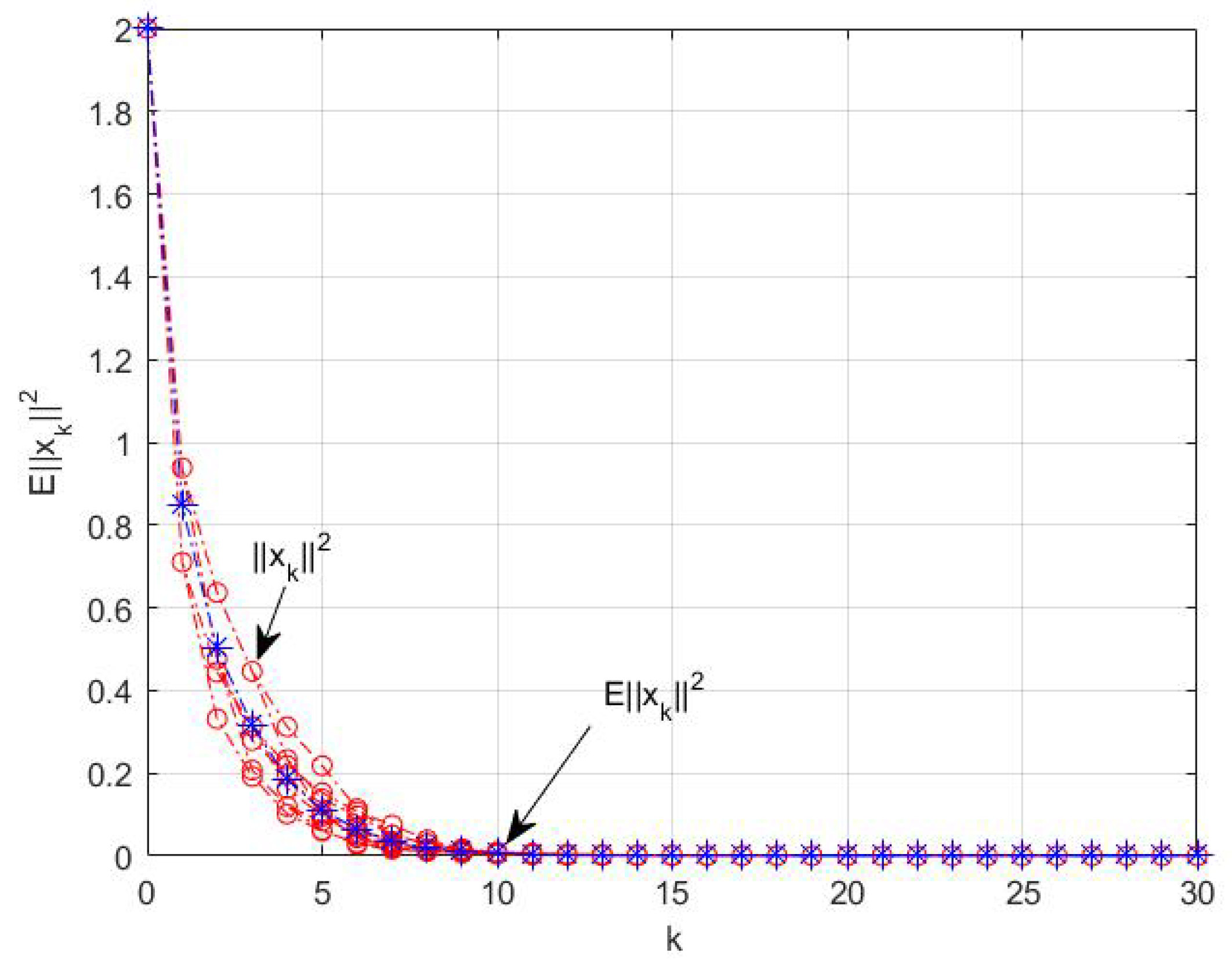
First, a mean-square strongly stable system is given, which can be verified by Theorem 1.

Example 1.

Consider a discrete-time Markov jump system (1) with two modes. The system parameters are given by

$$A_{0,1}=\left[\begin{array}{cc}0.2& -0.2\\ 0& -0.5\end{array}\right],A_{1,1}=\left[\begin{array}{cc}0.8& -0.2\\ 0& 0.4\end{array}\right],A_{2,1}=\left[\begin{array}{cc}0.1& 0.3\\ 0& 0.2\end{array}\right],$$

$$A_{0,2}=\left[\begin{array}{cc}0.2& -0.2\\ 0.2& -0.4\end{array}\right],A_{1,2}=\left[\begin{array}{cc}0.5& -0.2\\ -0.1& 0.4\end{array}\right],A_{2,2}=\left[\begin{array}{cc}0.2& 0.3\\ 0.1& 0.2\end{array}\right],$$

with initial distribution $q_1=0.5$, $q_2=0.5$, and the transition probability matrix

$${\left({\pi }_{ij}\right)}_{2\times 2}=\left[\begin{array}{cc}0.3& 0.7\\ 0.5& 0.5\end{array}\right].$$

According to Theorem 1, the following can be obtained:

$$\parallel {\mathcal{A}}_1\parallel =∥\begin{array}{c}{A}_{0,1}\\ A_{1,1}\\ A_{2,1}\end{array}∥=0.91<1,$$

and

$$\parallel {\mathcal{A}}_2\parallel =∥\begin{array}{c}{A}_{0,2}\\ A_{1,2}\\ A_{2,2}\end{array}∥=0.81<1.$$

Therefore, the system is mean-square strongly stable.

Taking $x\left(0\right)={[1-1]}^T$, the system state curves are shown in Figure 1. It can be seen that the norm of the system state is convergent.

Next, a system that is not mean-square strongly stable is given, and the design problems of the state feedback controller and output feedback controller are discussed.

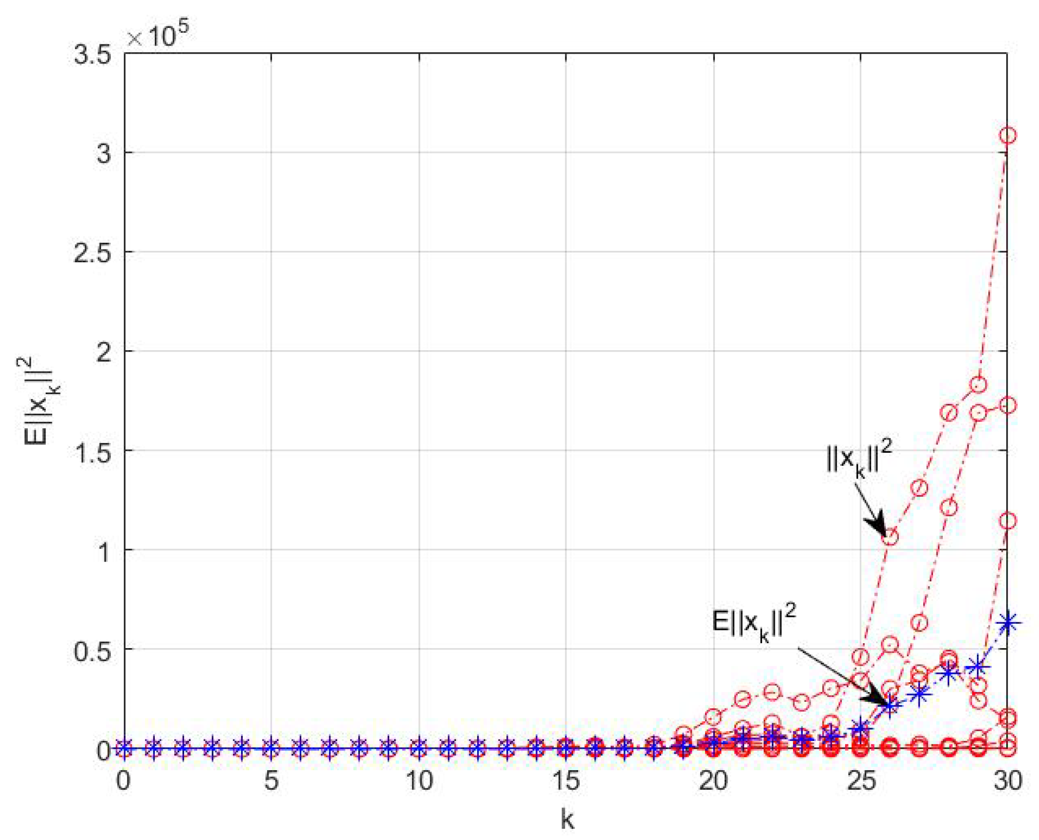
Example 2.

Consider a discrete-time Markov jump system (1) with two modes, where the parameters of the system are given by

$$A_{0,1}=\left[\begin{array}{cc}0.8& -0.5\\ 0.15& 0.9\end{array}\right],A_{1,1}=\left[\begin{array}{cc}0.2& -0.5\\ 0& 0.2\end{array}\right],A_{2,1}=\left[\begin{array}{cc}0.1& -0.8\\ 0& 0.1\end{array}\right],$$

$$B_{0,1}=\left[\begin{array}{ccc}0.6& -0.2& 0.5\\ -0.6& 0& 0.3\end{array}\right],B_{1,1}=\left[\begin{array}{ccc}0.3& 0.1& 0.3\\ 0& 0.5& 0\end{array}\right],B_{2,1}=\left[\begin{array}{ccc}0.2& 0.2& 0\\ 0& 0.8& 0.1\end{array}\right],$$

$$A_{0,2}=\left[\begin{array}{cc}0.85& -0.3\\ 0& 0.8\end{array}\right],A_{1,2}=\left[\begin{array}{cc}0.1& -0.5\\ 0.3& 0.1\end{array}\right],A_{2,2}=\left[\begin{array}{cc}0.1& 0.5\\ 0.5& 0.2\end{array}\right],$$

$$B_{0,2}=\left[\begin{array}{ccc}0.6& -0.2& 0.5\\ -0.6& 0& 0.3\end{array}\right],B_{1,2}=\left[\begin{array}{ccc}0.5& -0.1& 0.3\\ 0.1& 0.5& 0.1\end{array}\right],B_{2,2}=\left[\begin{array}{ccc}0.7& 0.2& 0.1\\ 0.1& 0.5& 0.1\end{array}\right],$$

with initial distribution $q_1=0.5$, $q_2=0.5$, and the transition probability matrix

$${\left({\pi }_{ij}\right)}_{2\times 2}=\left[\begin{array}{cc}0.3& 0.7\\ 0.5& 0.5\end{array}\right].$$

According to Theorem 1, the following can be obtained:

$$\parallel {\mathcal{A}}_1\parallel =∥\begin{array}{c}{A}_{0,1}\\ A_{1,1}\\ A_{2,1}\end{array}∥=1.46>1,$$

and

$$\parallel {\mathcal{A}}_2\parallel =∥\begin{array}{c}{A}_{0,2}\\ A_{1,2}\\ A_{2,2}\end{array}∥=1.16>1.$$

Therefore, the system is not mean-square strongly stable.

Taking $x\left(0\right)={[1-1]}^T$, the system state curves are shown in Figure 2. It can be seen that the norm of the system state is divergent.

Next, we consider the problems of mean-square strong stabilization by state feedback and output feedback with respect to Example 2.

Firstly, to consider the problems of state feedback controller design, the preconditions of (17) of Theorem 2 should be satisfied, and then the verification process is as follows.

According to Remark 4, the singular decomposition of ${\mathcal{B}}_i$ is as follows.

In mode 1:

$$U_{1,1}=\left[\begin{array}{ccc}& 0.55& 0.56\\ & -0.25& -0.38\\ & 0.11& 0.41\\ & -0.42& 0.27\\ & -0.07& 0.27\\ & -0.66& 0.47\end{array}\right],U_{1,2}=\left[\begin{array}{ccccc}& -0.40& 0.27& -0.05& 0.39\\ & -0.86& 0.07& 0.22& 0\\ & -0.26& -0.39& -0.08& -0.77\\ & 0.04& 0.79& -0.11& -0.32\\ & 0.15& -0.01& 0.95& -0.01\\ & -0.09& -0.38& -0.17& 0.39\end{array}\right],$$

$${\Sigma }_1=\left[\begin{array}{ccc}1& 0& 0\\ 0& 0.96& 0\\ 0& 0& 0.59\\ 0& 0& 0\\ 0& 0& 0\\ 0& 0& 0\end{array}\right],V_1=\left[\begin{array}{cccc}& 0.5& 0.78& 0.39\\ & -0.85& 0.52& 0.05\\ & 0.17& 0.36& -0.92\end{array}\right].$$

Then, we take

$${\mathcal{B}}_1^{\perp }=U_{1,2}^T,$$

and obtain

$${\mathcal{B}}_1^{\perp }(I-{\mathcal{A}}_1{\mathcal{A}}_1^T){\mathcal{B}}_1^{\perp T}=\left[\begin{array}{ccccc}& 0.44& 0.21& -0.27& 0.17\\ & 0.21& 0.91& 0.12& -0.07\\ & -0.27& 0.12& 0.71& 0.08\\ & 0.17& -0.07& 0.08& 0.95\end{array}\right],$$

which is a positive definite matrix because

$$\lambda \left({\mathcal{B}}_1^{\perp }(I-{\mathcal{A}}_1{\mathcal{A}}_1^T){\mathcal{B}}_1^{\perp T}\right)=\{0.15,0.87,1,1\}.$$

Hence, by testing the conditions that ${\mathcal{B}}_1$ has full column rank and

$${\mathcal{B}}_1^{\perp }(I-{\mathcal{A}}_1{\mathcal{A}}_1^T){\mathcal{B}}_1^{\perp T}>0$$

in Theorem 3, mode 1 satisfies the conditions of mean-square strong stabilization. Then, we can take

$$P_1=\left[\begin{array}{cc}0.5& 0\\ 0& 0.4\\ 0& 0.6\end{array}\right]$$

without loss of generality, and hence

$${\Theta }_1=\left[\begin{array}{cc}0.95& -0.03\\ -0.03& 0.63\end{array}\right],K_1=\left[\begin{array}{ccc}& 0.26& 1.35\\ & 0.13& 0.32\\ & -1.14& 0.33\end{array}\right]$$

from (18) and (19) in Theorem 3. According to Theorem 2, one obtains

$$\parallel {\mathcal{A}}_1+{\mathcal{B}}_1{K}_1\parallel =0.84<1.$$

In mode 2:

$$U_{2,1}=\left[\begin{array}{ccc}& -0.56& 0.36\\ & 0.38& 0.04\\ & -0.44& 0.2\\ & -0.12& -0.62\\ & -0.56& -0.22\\ & -0.12& -0.62\end{array}\right],U_{2,2}=\left[\begin{array}{ccccc}& -0.45& 0.35& -0.32& 0.35\\ & -0.8& -0.01& 0.46& -0.01\\ & -0.20& -0.6& -0.03& -0.60\\ & -0.22& 0.49& -0.22& -0.51\\ & 0.16& 0.12& 0.76& 0.12\\ & -0.22& -0.51& -0.22& 0.49\end{array}\right],$$

$${\Sigma }_2=\left[\begin{array}{ccc}1.26& 0& 0\\ 0& 0.77& 0\\ 0& 0& 0.58\\ 0& 0& 0\\ 0& 0& 0\\ 0& 0& 0\end{array}\right],V_2=\left[\begin{array}{cccc}& -0.95& 0.02& 0.31\\ & -0.06& -0.99& -0.12\\ & -0.30& 0.14& -0.94\end{array}\right].$$

Then, we take

$${\mathcal{B}}_2^{\perp }=U_{2,2}^T,$$

and obtain

$${\mathcal{B}}_2^{\perp }(I-{\mathcal{A}}_2{\mathcal{A}}_2^T){\mathcal{B}}_2^{\perp T}=\left[\begin{array}{ccccc}& 0.54& 0.15& 0.1& 0.3\\ & 0.15& 0.94& -0.1& -0.1\\ & 0.1& -0.1& 0.22& -0.1\\ & 0.3& -0.1& -0.11& 0.8\end{array}\right],$$

which is a positive definite matrix because

$$\lambda \left({\mathcal{B}}_2^{\perp }(I-{\mathcal{A}}_1{\mathcal{A}}_1^T){\mathcal{B}}_1^{\perp T}\right)=\{0.08,0.41,1,1\}.$$

Hence, by testing the conditions that ${\mathcal{B}}_2$ has full column rank and

$${\mathcal{B}}_2^{\perp }(I-{\mathcal{A}}_2{\mathcal{A}}_2^T){\mathcal{B}}_2^{\perp T}>0$$

in Theorem 3, mode 2 satisfies the conditions for mean-square strong stabilization. Then, we can take

$$P_2=\left[\begin{array}{cc}0.4& 0\\ 0& 0.7\\ 0.4& 0.1\end{array}\right]$$

without loss of generality, and hence

$${\Theta }_2=\left[\begin{array}{cc}0.72& 0.18\\ 0.18& 0.24\end{array}\right],K_2=\left[\begin{array}{ccc}& -0.01& 0.51\\ & -0.28& -0.25\\ & -0.55& -0.29\end{array}\right]$$

from (18) and (19) in Theorem 3. According to Theorem 2, one obtains

$$\parallel {\mathcal{A}}_2+{\mathcal{B}}_2{K}_2\parallel =0.95<1.$$

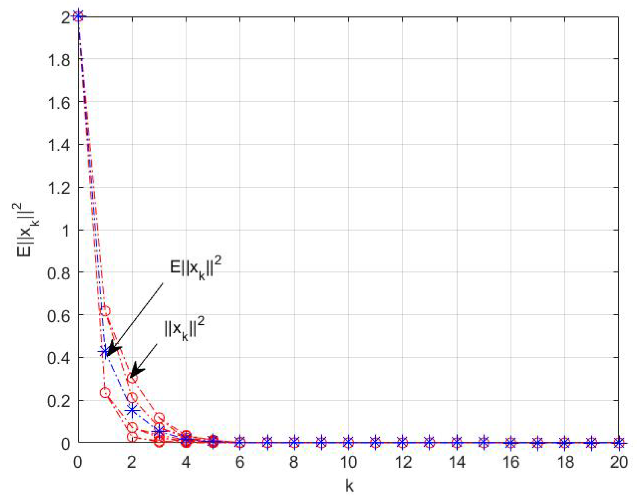
Taking $x\left(0\right)={[1-1]}^T$, the closed-loop system state curves are shown in Figure 3. It can be seen that the system is mean-square strongly stabilized via state feedback control.

Next, we consider the problem of designing the static output feedback controller in the above example. First, we consider Example 2 with the output matrices $C_i$ as follows:

$$C_1=\left[\begin{array}{cc}1& 1\\ 0& 1\end{array}\right],C_2=\left[\begin{array}{cc}0.2& 0.8\\ 1& 0.1\end{array}\right].$$

According to the above analysis, the system in Example 2 also satisfies the condition of (30) in Theorem 5. Hence, we only need to verify condition (31) in Theorem 5. As C and $\widehat{C}$ are square matrices, we consider the following procedure:

$$C_1^T{C}_1=\left[\begin{array}{cc}1& 1\\ 1& 2\end{array}\right],C_2^T{C}_2=\left[\begin{array}{cc}1& 1\\ 1& 2\end{array}\right],$$

The eigenvalues of the above matrices are $\{0.38,2.62\}$ $,\{0.52,1.17\}$, respectively, and $C_1^T{C}_1>0$, $C_2^T{C}_2>0$. Hence we can design the output feedback controller for this system using Theorem 5, according to (32)–(34), and taking matrices $L_i$ as

$$L_1=\left[\begin{array}{cc}0.5& -0.2\\ -0.1& 0\\ 0.3& 0.3\end{array}\right],L_2=\left[\begin{array}{cc}0.5& 0.1\\ 0.2& 0.2\\ 0.4& -0.1\end{array}\right],$$

without loss of generality. The explicit expressions for output feedback controllers can be obtained as follows:

$${\Psi }_1=\left[\begin{array}{cc}0.95& -0.98\\ -0.98& 1.63\end{array}\right],F_1=\left[\begin{array}{cc}0.26& 1.17\\ 0.05& -0.08\\ -0.98& 1.63\end{array}\right],$$

$${\Psi }_2=\left[\begin{array}{cc}0.24& 0.66\\ 0.66& 0.68\end{array}\right],F_2=\left[\begin{array}{cc}0.86& -0.24\\ -0.66& -0.02\\ -0.15& -1.06\end{array}\right].$$

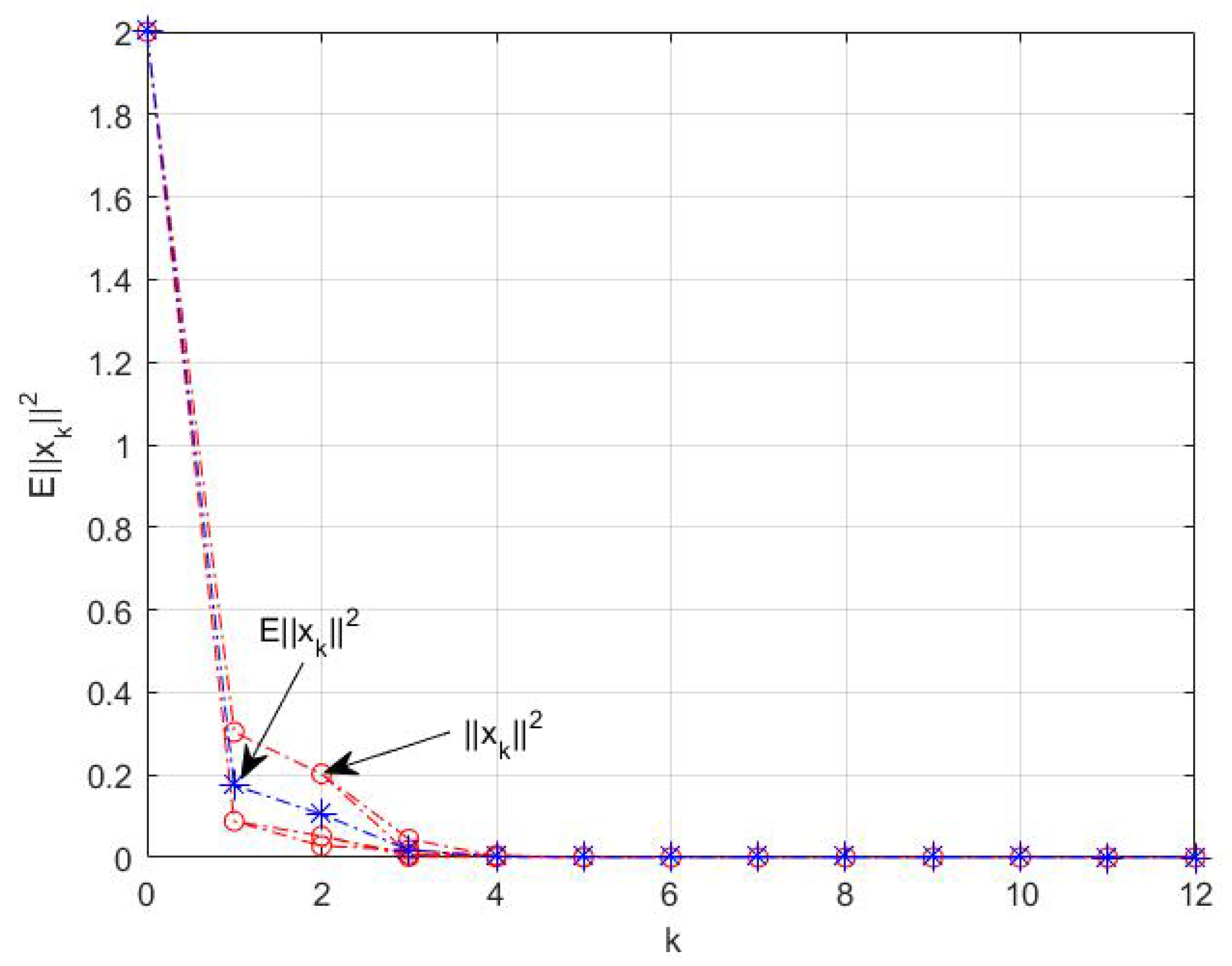
Taking $x\left(0\right)={[1-1]}^T$, the closed-loop system curves are shown in Figure 4. It can be seen that the system is mean-square strongly stabilized via output feedback control.

6. Conclusions

In this paper, the definition of the mean-square strong stability of discrete-time Markov jump systems was proposed, and the necessary and sufficient conditions for mean-square strong stability were obtained. Furthermore, several necessary and sufficient conditions guaranteeing mean-square strong stabilization via a state feedback controller and a static output feedback controller were derived. Moreover, the explicit expressions for the state feedback controller and static output feedback controller were provided. In future work, the conclusions of this paper could be extended to a broader context such as semi-Markov jump systems, monotone evolutions for the state vectors, and so on. In addition, Theorems 3 and 5 can also be optimized for some aspects, in order to obtain a broader conclusion.