Advanced Study on the Delay Differential Equation y′(t) = ay(t) + by(ct)

Abstract

Many real-world problems have been modeled via delay differential equations. The pantograph delay differential equation $y^{\prime }\left(t\right)=ay\left(t\right)+by\left(ct\right)$ belongs to such a set of delay differential equations. To the authors’ knowledge, there are no standard methods to solve the delay differential equations, i.e., unlike the ordinary differential equations, for which numerous and standard methods are well-known. In this paper, the Adomian decomposition method is suggested to analyze the pantograph delay differential equation utilizing two different canonical forms. A power series solution is obtained through the first canonical form, while the second canonical form leads to the exponential function solution. The obtained power series solution coincides with the corresponding ones in the literature for special cases. Moreover, several exact solutions are derived from the present power series solution at a specific restriction of the proportional delay parameter c in terms of the parameters a and b. The exponential function solution is successfully obtained in a closed form and then compared with the available exact solutions (derived from the power series solution). The obtained results reveal that the present analysis is efficient and effective in dealing with pantograph delay differential equations.

1. Introduction

The device that maintains electrical contact with the contact wire and transfers power from the wire to the traction unit used in electric locomotives and trams is also called a pantograph [1]. Although the pantograph problem has been addressed by many authors [2,3,4,5,6,7,8,9,10,11], it still needs a considerable effort to search for further/undiscovered properties, which will be revealed through the present study. Indeed, the ordinary differential equations (ODEs) are used to describe numerous physical phenomena; however, the actual behavior of other phenomena can be accurately modeled via imposing nonlocal components such as delays. For this reason, the delay differential equations (DDEs) have become an ideal alternative to ODEs for formulating many mathematical models [10]. Finding solutions for the DDEs is not an easy task, in contrast to the ODEs. Perhaps the reason is that there are no specific methods to solve DDEs, and consequently, it becomes a challenge for mathematicians. Certainly, such a challenge increases if our goal is to reach the exact or the closed-form solution for DDEs. This is the main incentive for re-examining the PDDE [2,3,4,5,6,7,8,9,10,11]:

$$y^{\prime }\left(t\right)=ay\left(t\right)+by\left(ct\right),y\left(0\right)=\lambda ,b\ne 0,c\ne 1.$$

(1)

In Refs. [2,3,4,5,6,7,8,9,10,11], PDDE (1) has been studied using differential analysis. However, PDDE (1) still needs further efforts to determine its exact/closed-form solution for all possible real values of the proportional delay parameter c. A special case of the PDDE is called the Ambartsumian delay differential equation (ADDE) when $a=-1$ and $b=c=\frac{1}{q}$ ($q>1$). The ADDE, in both classical and generalized forms, describes the surface brightness in the Milky Way [12,13,14,15,16,17,18,19,20,21].

Very recently, the authors in Ref. [22] determined the exact solution for the PDDE when $c=-1$. They showed that the solution is periodic and hyperbolic if $b>a$ and $a>b$, respectively. Additionally, they derived a truncated series solution in the case $a=b$ ($c=-1$). The objective of this paper is to obtain two different analytic forms for the solution of the PDDE. This target can be achieved by using a relatively recent series method such as the Adomian decomposition method (ADM) [23,24,25,26,27,28,29,30,31,32,33,34,35,36,37]. Additionally, other techniques were found to be effective in solving integral and differential equations as discussed by the authors [38,39,40] and for the nonlinear structures of the pantograph models in Refs. [41,42]. However, the ADM is chosen in this paper as an effective tool to treat the PDDE where two different canonical forms are constructed. We declare in this paper that the first canonical form leads to the standard power series solution (PSS), while the second is the exponential function solution (EFS), which is determined in a closed form. The characteristics of both the PSS and the EFS are addressed in detail. In addition, the efficiency of the EFS is validated through various comparisons with the exact solutions, which are derived from the PSS via a basic theorem in this paper.

The paper is structured as follows. In Section 2, the PSS is analyzed via the first canonical form. Some known results in the literature are recovered in Section 2 as special cases of the PSS. Section 3 is devoted to obtaining the EFS using the second canonical form. The properties of the EFS components are addressed in Section 4. A unified formula for the general component is derived in Section 5 through a theorem. The validity of such a unified formula is proved in Section 6. Accordingly, a closed form is determined for the EFS in Section 7. In addition, the exact solutions for some special cases are evaluated in Section 8. Finally, the results are discussed in detail in Section 9 and concluded in Section 10.

2. The PSS Canonical Form

In order to apply the ADM to solve Equation (1), we first integrate both sides with respect to t which yields

$${\int }_0^t{y}^{\prime }\left(\tau \right)d\tau ={\int }_0^t\left[ay\left(\tau \right)+by\left(c\tau \right)\right]d\tau ,$$

(2)

i.e.,

$$y\left(t\right)-y\left(0\right)={\int }_0^t\left[ay\left(\tau \right)+by\left(c\tau \right)\right]d\tau ,$$

(3)

or

$$y\left(t\right)=y\left(0\right)+{\int }_0^t\left[ay\left(\tau \right)+by\left(c\tau \right)\right]d\tau .$$

(4)

Utilizing the initial condition $y\left(0\right)=\lambda$, Equation (4) then takes the canonical form:

$$y\left(t\right)=\lambda +{\int }_0^t\left[ay\left(\tau \right)+by\left(c\tau \right)\right]d\tau .$$

(5)

The ADM assumes $y\left(t\right)$ in the form:

$$y\left(t\right)=\sum _{i=0}^{\infty }{y}_i\left(t\right).$$

(6)

The convergence of the series in Equation (6) was extensively discussed by the authors in Refs. [23,33,34]. Inserting (6) into (5) yields

$$\sum _{i=0}^{\infty }{y}_i\left(t\right)=\lambda +{\int }_0^t\left[a\sum _{i=0}^{\infty }{y}_i\left(\tau \right)+b\sum _{i=0}^{\infty }{y}_i\left(c\tau \right)\right]d\tau ,$$

(7)

or

$$y_0\left(t\right)+\sum _{i=1}^{\infty }{y}_i\left(t\right)=\lambda +\sum _{i=0}^{\infty }{\int }_0^t\left[a{y}_i\left(\tau \right)+b{y}_i\left(c\tau \right)\right]d\tau .$$

(8)

In Equations (7) and (8), the order of integration and series is changed under the assumptions that all $y_i$ are continuous and non-negative functions, i.e.,

$$y_0\left(t\right)+\sum _{i=1}^{\infty }{y}_i\left(t\right)=\lambda +\sum _{i=1}^{\infty }{\int }_0^t\left[a{y}_{i-1}\left(\tau \right)+b{y}_{i-1}\left(c\tau \right)\right]d\tau .$$

(9)

Hence,

$$\begin{array}{cc}\hfill y_0\left(t\right)& =\lambda ,\hfill \\ \hfill y_i\left(t\right)& ={\int }_0^t\left[a{y}_{i-1}\left(\tau \right)+b{y}_{i-1}\left(c\tau \right)\right]d\tau ,i\ge 1.\hfill \end{array}$$

(10)

Therefore,

$$\begin{array}{cc}\hfill y_1& ={\int }_0^t\left[a{y}_0\left(\tau \right)+b{y}_0\left(c\tau \right)\right]d\tau ={\int }_0^t\left(a\lambda +b\lambda \right)d\tau =\lambda (a+b)t,\hfill \end{array}$$

(11)

$$\begin{array}{cc}\hfill y_2& ={\int }_0^t\left[a{y}_1\left(\tau \right)+b{y}_1\left(c\tau \right)\right]d\tau ={\int }_0^t\left[a\lambda (a+b)\tau +b\lambda (a+b)c\tau \right]d\tau \hfill \\ \hfill & =\lambda (a+b)(a+bc){\displaystyle \frac{t^2}{2!}}=\lambda \prod _{k=1}^2\left(a+b{c}^{k-1}\right){\displaystyle \frac{t^2}{2!}}.\hfill \end{array}$$

(12)

Similarly, we obtain

$$\begin{array}{cc}\hfill y_3& =\lambda (a+b)(a+bc)(a+b{c}^2){\displaystyle \frac{t^3}{3!}}=\lambda \prod _{k=1}^3\left(a+b{c}^{k-1}\right){\displaystyle \frac{t^3}{3!}},\hfill \end{array}$$

(13)

$$\begin{array}{cc}\hfill y_4& =\lambda (a+b)(a+bc)(a+b{c}^2)(a+b{c}^3){\displaystyle \frac{t^4}{4!}}=\lambda \prod _{k=1}^4\left(a+b{c}^{k-1}\right){\displaystyle \frac{t^4}{4!}},\hfill \\ \hfill ⋮\end{array}$$

(14)

$$\begin{array}{cc}\hfill y_i& =\lambda (a+b)(a+bc)(a+b{c}^2)\cdots (a+b{c}^{i-1}){\displaystyle \frac{t^i}{i!}}=\lambda \prod _{k=1}^i\left(a+b{c}^{k-1}\right){\displaystyle \frac{t^i}{i!}}.\hfill \end{array}$$

(15)

Thus,

$$\begin{array}{cc}\hfill y\left(t\right)& =y_0+\sum _{i=1}^{\infty }{y}_i,\hfill \\ \hfill & =\lambda +\lambda \sum _{i=1}^{\infty }\prod _{k=1}^i\left(a+b{c}^{k-1}\right){\displaystyle \frac{t^i}{i!}},\hfill \\ \hfill & =\lambda \left[1+\sum _{i=1}^{\infty }\left(\prod _{k=1}^i\left(a+b{c}^{k-1}\right)\right){\displaystyle \frac{t^i}{i!}}\right].\hfill \end{array}$$

(16)

At $\lambda =1$, the solution to (16) becomes

$$y\left(t\right)=1+\sum _{i=1}^{\infty }\left(\prod _{k=1}^i\left(a+b{c}^{k-1}\right)\right){\displaystyle \frac{t^i}{i!}},$$

(17)

which is the same closed-form series solution obtained by Fox et al. [11]. In addition, if $a=-1$ and $b=c=\frac{1}{q}$, $q>1$, the IVP (1) becomes

$$y^{\prime }\left(t\right)=-y\left(t\right)+\frac{1}{q}y\left(\frac{t}{q}\right),y\left(0\right)=\lambda ,$$

(18)

which is the ADDE in Refs. [12,13,14,15,16,17,43]. Substituting $a=-1$ and $b=c=\frac{1}{q}$ into (17) gives

$$y\left(t\right)=\lambda \left[1+\sum _{i=1}^{\infty }\left(\prod _{k=1}^i\left(-1+q^{-k}\right)\right){\displaystyle \frac{t^i}{i!}}\right],$$

(19)

i.e.,

$$y\left(t\right)=\lambda \left[1+\sum _{i=1}^{\infty }\left(\prod _{k=1}^i\left(q^{-k}-1\right)\right){\displaystyle \frac{t^i}{i!}}\right],$$

(20)

which is the corresponding PSS obtained in Refs. [12,15].

3. The EFS Canonical Form

Equation (1) can be rewritten in the following canonical form:

$$y\left(t\right)=\lambda e^{at}+b{e}^{at}{\int }_0^t{e}^{-a\tau }y\left(c\tau \right)d\tau .$$

(21)

The method of obtaining Equation (21) is to transform Equation (1) to an equivalent integral form. This task can be achieved by solving Equation (1) as a first-order linear ODE by means of the integrating factor. On inserting (6) into (21), we obtain

$$\sum _{i=0}^{\infty }{y}_i\left(t\right)=\lambda e^{at}+b{e}^{at}{\int }_0^t{e}^{-a\tau }\sum _{i=0}^{\infty }{y}_i\left(c\tau \right)d\tau ,$$

(22)

or

$$y_0\left(t\right)+\sum _{i=1}^{\infty }{y}_i\left(t\right)=\lambda e^{at}+\sum _{i=1}^{\infty }b{e}^{at}{\int }_0^t{e}^{-a\tau }{y}_{i-1}\left(c\tau \right)d\tau ,$$

(23)

and hence, we have the following recurrence scheme:

$$\begin{array}{ccc}& & y_0\left(t\right)=\lambda e^{at},\hfill \\ & & y_i\left(t\right)=b{e}^{at}{\int }_0^t{e}^{-a\tau }{y}_{i-1}\left(c\tau \right)d\tau ,i\ge 1.\hfill \end{array}$$

(24)

For $i=1$, Equation (24) gives

$$y_1\left(t\right)=b{e}^{at}{\int }_0^t{e}^{-a\tau }{y}_0\left(c\tau \right)d\tau =\lambda b{e}^{at}{\int }_0^t{e}^{a(c-1)\tau }d\tau ,$$

(25)

where $y_0\left(c\tau \right)=\lambda e^{ac\tau }$. Performing the integral in (25), we obtain

$$y_1\left(t\right)=\frac{\lambda b}{a(c-1)}\left(e^{act}-e^{at}\right),a\ne 0,c\ne 1.$$

(26)

Similarly, at $i=2$, we have

$$y_2\left(t\right)=b{e}^{at}{\int }_0^t{e}^{-a\tau }{y}_1\left(c\tau \right)d\tau =\frac{\lambda b^2}{a(c-1)}{e}^{at}{\int }_0^t\left(e^{a(c^2-1)\tau }-e^{a(c-1)\tau }\right)d\tau ,$$

(27)

which implies

$$y_2\left(t\right)=\frac{\lambda b^2}{a(c-1)}{e}^{at}\left(\frac{e^{a(c^2-1)t}}{a(c^2-1)}-\frac{e^{a(c-1)t}}{a(c-1)}-\left(\frac{1}{a(c^2-1)}-\frac{1}{a(c-1)}\right)\right).$$

(28)

Simplifying (28) yields

$$y_2\left(t\right)=\frac{\lambda b^2}{a^2(c-1)(c^2-1)}\left(e^{a{c}^{2}t}-(c+1)e^{act}+c{e}^{at}\right),a\ne 0,c\ne \pm 1.$$

(29)

Repeating the procedure above for $i=3$, then

$$\begin{array}{cc}\hfill y_3\left(t\right)& =b{e}^{at}{\int }_0^t{e}^{-a\tau }{y}_2\left(c\tau \right)d\tau \hfill \\ \hfill & =\frac{\lambda b^3}{a^2(c-1)(c^2-1)}{\int }_0^t\left(e^{a(c^3-1)\tau }-(c+1)e^{a(c^2-1)\tau }+c{e}^{a(c-1)\tau }\right)d\tau .\hfill \end{array}$$

(30)

Evaluating this integral and simplifying, we then get

$$y_3\left(t\right)=\frac{\lambda b^3}{a^3(c-1)(c^2-1)(c^3-1)}\left(e^{a{c}^{3}t}-(c^2+c+1)e^{a{c}^{2}t}+(c^3+c^2+c)e^{act}-c^3{e}^{at}\right).$$

(31)

The higher-order components of Adomian’s series can also be calculated through any software such as Mathematica. Moreover, a general formula for finding the $i\mathrm{th}$-component $y_i$, $\forall i\ge 1$ will be obtained in a subsequent section. Before doing so, it may be reasonable to address some observations about the properties of the components $y_1$, $y_2$, and $y_3$. Such properties are to be analyzed in the next section, and hence, we will have the opportunity to obtain a general formula for the $y_i$ component $\forall i\ge 1$.

4. Properties of the EFS

From the analysis of the previous section, it is observed that

• The number of terms involved in each component exceeds the order of such component by one. For example, the components $y_1\left(t\right)$, $y_2\left(t\right)$, and $y_3\left(t\right)$ contain two terms, three terms, and four terms, respectively;
• The two terms contained in $y_1\left(t\right)$ are in the forms ${\sigma }_{1,0}{e}^{at}$ and ${\sigma }_{1,1}{e}^{act}$, where ${\sigma }_{1,0}$ and ${\sigma }_{1,1}$ are the coefficients of $e^{at}$ and $e^{act}$ given by ${\sigma }_{1,0}=-\frac{\lambda b}{a(c-1)}$ and ${\sigma }_{1,1}=\frac{\lambda b}{a(c-1)}$, respectively. This means that $y_1\left(t\right)$ can be written as $y_1\left(t\right)={\sum }_{m=0}^1{\sigma }_{1,m}{e}^{a{c}^{m}t}$. Similarly, $y_2\left(t\right)$ can be written as $y_2\left(t\right)={\sum }_{m=0}^2{\sigma }_{2,m}{e}^{a{c}^{m}t}={\sigma }_{2,0}{e}^{at}+{\sigma }_{2,1}{e}^{act}+{\sigma }_{2,2}{e}^{a{c}^{2}t}$, where ${\sigma }_{2,0}=\frac{\lambda b^{2}c}{a^2(c-1)(c^2-1)}$, ${\sigma }_{2,1}=-\frac{\lambda b^2(c+1)}{a^2(c-1)(c^2-1)}=-\frac{\lambda b^2}{a^2{(c-1)}^2}$, and ${\sigma }_{2,2}=\frac{\lambda b^2}{a^2(c-1)(c^2-1)}$. Additionally, we have $y_3\left(t\right)={\sum }_{m=0}^3{\sigma }_{3,m}{e}^{a{c}^{m}t}={\sigma }_{3,0}{e}^{at}+{\sigma }_{3,1}{e}^{act}+{\sigma }_{3,2}{e}^{a{c}^{2}t}+{\sigma }_{3,3}{e}^{a{c}^{3}t}$, where ${\sigma }_{3,0}=-\frac{\lambda b^3{c}^3}{a^3(c-1)(c^2-1)(c^3-1)}$, ${\sigma }_{3,1}=\frac{\lambda b^3{c}^3(c^3+c^2+c)}{a^3(c-1)(c^2-1)(c^3-1)}=\frac{\lambda b^3{c}^4}{a^3{(c-1)}^2(c^2-1)}$, ${\sigma }_{3,2}=-\frac{\lambda b^3{c}^3(c^2+c+1)}{a^3(c-1)(c^2-1)(c^3-1)}=-\frac{\lambda b^3{c}^3}{a^3{(c-1)}^2(c^2-1)}$, and ${\sigma }_{3,3}=\frac{\lambda b^3}{a^3(c-1)(c^2-1)(c^3-1)}$;
• It is noted from the above that the sum of the coefficients of any of these components vanishes. For example, we have ${\sigma }_{1,0}+{\sigma }_{1,1}=0$ for the component $y_1\left(t\right)$, ${\sigma }_{2,0}+{\sigma }_{2,1}+{\sigma }_{2,2}=0$ for $y_2\left(t\right)$, and ${\sigma }_{3,0}+{\sigma }_{3,1}+{\sigma }_{3,2}+{\sigma }_{3,3}=0$ for $y_3\left(t\right)$;
• Based on these observations, the general component $y_i\left(t\right)$ takes the form $y_i\left(t\right)={\sum }_{m=0}^i{\sigma }_{i,m}{e}^{a{c}^{m}t}$$\forall i\ge 1$. Additionally, note that the initial component $y_0\left(t\right)={\sum }_{m=0}^0{\sigma }_{0,m}{e}^{a{c}^{m}t}={\sigma }_{0,0}{e}^{at}$ with ${\sigma }_{0,0}=\lambda$. The next section considers an attempt to determine a general form of the coefficients ${\sigma }_{i,m}$; hence, a closed-form solution is expected. It will also be proved that the sum of the coefficients of any component $y_i\left(t\right)$ vanishes, i.e., ${\sum }_{m=0}^i{\sigma }_{i,m}=0$$\forall i\ge 1$.

5. General-Component Formula for the EFS

Theorem 1.

The general component $y_i\left(t\right)$ of Adomian’s series is given by

$$y_i\left(t\right)=\sum _{m=0}^i{\sigma }_{i,m}{e}^{a{c}^{m}t},$$

(32)

where

$${\sigma }_{i,m+1}=\frac{b{\sigma }_{i-1,m}}{a(c^{m+1}-1)},{\sigma }_{i,0}=-\sum _{m=0}^{i-1}\frac{b{\sigma }_{i-1,m}}{a(c^{m+1}-1)},m\ge 0,i\ge 1,$$

(33)

and the following property holds $\forall m\ge 0,i\ge 1$:

$$\sum _{m=0}^i{\sigma }_{i,m}=0.$$

(34)

Proof. 

In view of the above properties, discussed in the previous section, the component $y_i\left(t\right)$ can be assumed in the form:

$$y_i\left(t\right)=\sum _{m=0}^i{\sigma }_{i,m}{e}^{a{c}^{m}t}.$$

(35)

Substituting (35) into the canonical form (24) yields

$$\sum _{m=0}^i{\sigma }_{i,m}{e}^{a{c}^{m}t}=b{e}^{at}{\int }_0^t{e}^{-a\tau }\sum _{m=0}^{i-1}{\sigma }_{i-1,m}{e}^{a{c}^{m+1}\tau }d\tau ,i\ge 1,$$

(36)

or

$${\sigma }_{i,0}{e}^{at}+\sum _{m=1}^i{\sigma }_{i,m}{e}^{a{c}^{m}t}=\sum _{m=0}^{i-1}b{\sigma }_{i-1,m}{e}^{at}{\int }_0^t{e}^{a(c^{m+1}-1)\tau }d\tau ,$$

(37)

i.e.,

$${\sigma }_{i,0}{e}^{at}+\sum _{m=0}^i{\sigma }_{i,m}{e}^{a{c}^{m+1}t}=\sum _{m=0}^{i-1}\frac{b{\sigma }_{i-1,m}}{a(c^{m+1}-1)}\left(e^{a{c}^{m+1}t}-e^{at}\right),$$

(38)

and hence,

$${\sigma }_{i,0}{e}^{at}+\sum _{m=0}^i{\sigma }_{i,m}{e}^{a{c}^{m+1}t}=\sum _{m=0}^{i-1}\frac{b{\sigma }_{i-1,m}}{a(c^{m+1}-1)}{e}^{a{c}^{m+1}t}-e^{at}\sum _{m=0}^{i-1}\frac{b{\sigma }_{i-1,m}}{a(c^{m+1}-1)}.$$

(39)

Comparing both sides, we obtain

$${\sigma }_{i,m+1}=\frac{b{\sigma }_{i-1,m}}{a(c^{m+1}-1)},{\sigma }_{i,0}=-\sum _{m=0}^{i-1}\frac{b{\sigma }_{i-1,m}}{a(c^{m+1}-1)}.$$

(40)

Combining the relations in (40) gives

$${\sigma }_{i,0}=-\sum _{m=0}^{i-1}{\sigma }_{i,m+1},$$

(41)

or

$${\sigma }_{i,0}+\sum _{m=1}^i{\sigma }_{i,m}=0,$$

(42)

and thus

$$\sum _{m=0}^i{\sigma }_{i,m}=0,\forall i\ge 1,$$

(43)

which completes the proof. □

6. Verification

Here, the general form of $y_i\left(t\right)$ is to be verified. For $i=1$, we have from (32) that

$$y_1\left(t\right)={\sigma }_{1,0}{e}^{at}+{\sigma }_{1,1}{e}^{act},$$

(44)

where ${\sigma }_{1,0}$ and ${\sigma }_{1,1}$ are to be determined using (33) as follows. Let $i=1$ and $m=0$; then

$${\sigma }_{1,1}=\frac{b{\sigma }_{0,0}}{a(c-1)},{\sigma }_{1,0}=-\frac{b{\sigma }_{0,0}}{a(c-1)},$$

(45)

i.e.,

$${\sigma }_{1,1}=\frac{b\lambda }{a(c-1)},{\sigma }_{1,0}=-\frac{b\lambda }{a(c-1)}.$$

(46)

Inserting (46) yields the same expression of the first component $y_1\left(t\right)$ given in (26). Similarly, at $i=2$, we have

$$y_2\left(t\right)={\sigma }_{2,0}{e}^{at}+{\sigma }_{2,1}{e}^{act}+{\sigma }_{2,2}{e}^{a{c}^{2}t}.$$

(47)

From the second relation in (33), we have at $i=2$ that

$${\sigma }_{2,0}=-\sum _{m=0}^1\frac{b{\sigma }_{1,m}}{a(c^{m+1}-1)}=-\frac{b{\sigma }_{1,0}}{a(c^{}-1)}-\frac{b{\sigma }_{1,1}}{a(c^2-1)},$$

(48)

where ${\sigma }_{1,0}$ and ${\sigma }_{1,1}$ were already obtained in (46); hence,

$${\sigma }_{2,0}=\frac{\lambda b^{2}c}{a^2(c-1)(c^2-1)}.$$

(49)

Moreover, at $i=2$ and $m=0$, the first relation in (33) gives

$${\sigma }_{2,1}=\frac{b{\sigma }_{1,0}}{a(c^{}-1)}=-\frac{\lambda b^2}{a^2{(c-1)}^2},$$

(50)

and for $i=2$ and $m=1$, we have

$${\sigma }_{2,2}=\frac{b{\sigma }_{1,1}}{a(c^2-1)}=-\frac{\lambda b^2}{a^2{(c-1)}^2}=\frac{\lambda b^2}{a^2(c-1)(c^2-1)}.$$

(51)

Substituting (49)–(51) into (47), we obtain the same $y_2\left(t\right)$ in (29). Following the above analysis, other components of higher order can be evaluated. Furthermore, the relations (33) can be easily programmed through any software.

7. The Closed-Form EFS

The objective of this section is to obtain the solution of Equation (1) in a closed form. Regarding this, we begin by rewriting Equation (32) in the form:

$$\begin{array}{cc}\hfill y_i\left(t\right)& ={\sigma }_{i,0}{e}^{at}+\sum _{m=1}^i{\sigma }_{i,m}{e}^{a{c}^{m}t}\hfill \\ \hfill & ={\sigma }_{i,0}{e}^{at}+\sum _{m=0}^{i-1}{\sigma }_{i,m+1}{e}^{a{c}^{m+1}t}.\hfill \end{array}$$

(52)

Implementing the relations (33) provided by Theorem 1 yields

$$y_i\left(t\right)=-\sum _{m=0}^{i-1}\frac{b{\sigma }_{i-1,m}}{a(c^{m+1}-1)}{e}^{at}+\sum _{m=0}^{i-1}\frac{b{\sigma }_{i-1,m}}{a(c^{m+1}-1)}{e}^{a{c}^{m+1}t}.$$

(53)

Therefore,

$$y_i\left(t\right)=\sum _{m=0}^{i-1}\frac{b{\sigma }_{i-1,m}}{a(c^{m+1}-1)}\left(e^{a{c}^{m+1}t}-e^{at}\right),$$

(54)

or

$$y_i\left(t\right)=\sum _{m=1}^i\frac{b{\sigma }_{i-1,m-1}}{a(c^m-1)}\left(e^{a{c}^{m}t}-e^{at}\right),i\ge 1.$$

(55)

Thus,

$$\begin{array}{cc}\hfill y\left(t\right)& =y_0\left(t\right)+\sum _{i=1}^{\infty }{y}_i\left(t\right)\hfill \\ \hfill & =\lambda e^{at}+\sum _{i=1}^{\infty }\sum _{m=1}^i\frac{b{\sigma }_{i-1,m-1}}{a(c^m-1)}\left(e^{a{c}^{m}t}-e^{at}\right),\hfill \end{array}$$

(56)

which is equivalent to

$$y\left(t\right)=\left(\lambda -\sum _{i=1}^{\infty }\sum _{m=1}^i\frac{b{\sigma }_{i-1,m-1}}{a(c^m-1)}\right)e^{at}+\sum _{i=1}^{\infty }\sum _{m=1}^i\frac{b{\sigma }_{i-1,m-1}}{a(c^m-1)}{e}^{a{c}^{m}t}.$$

(57)

8. Exact Solutions: Special Cases of the PSS

In this section, it is shown that the closed-form PSS (16) reduces to exact solutions at special cases of the parameters a, b, and c. The following theorem addresses this point.

Theorem 2.

For $r\in {\mathbb{N}}^{+}$ such that $(a+b{c}^r)=0$ (i.e., $c=\sqrt[r]{-\frac{a}{b}}$), the non-trivial exact solution of Equation (1) is given by

$$y\left(t\right)=\lambda \left[1+\sum _{i=1}^r\left(\prod _{k=1}^i\left(a+b{\left(-\frac{a}{b}\right)}^{\frac{k-1}{r}}\right)\right){\displaystyle \frac{t^i}{i!}}\right].$$

(58)

Proof. 

From (16), we can write

$$y\left(t\right)=\lambda \left[1+(a+b)t+(a+b)(a+bc)\frac{t^2}{2!}+(a+b)(a+bc)(a+b{c}^2)\frac{t^3}{3!}+\dots \right].$$

(59)

If $a+b=0$, then Equation (59) gives the trivial solution $y\left(t\right)=\lambda$. For $a+bc=0$ ($c=-\frac{a}{b}$), the infinite series (59) reduces to the exact solution

$$y\left(t\right)=\lambda \left[1+(a+b)t\right]=\lambda \left[1+\sum _{i=1}^1\left(\prod _{k=1}^1\left(a+b{\left(-\frac{a}{b}\right)}^{\frac{k-1}{1}}\right)\right){\displaystyle \frac{t^i}{i!}}\right].$$

(60)

Additionally, for $a+b{c}^2=0$ ($c=\sqrt{-\frac{a}{b}}$), the infinite series (59) reduces to

$$\begin{array}{cc}\hfill y\left(t\right)& =\lambda \left[1+(a+b)t+(a+b)(a+bc)\frac{t^2}{2!}\right]\hfill \\ \hfill & =\lambda \left[1+(a+b)t+(a+b)\left(a+b{\left(-\frac{a}{b}\right)}^{\frac{1}{2}}\right)\frac{t^2}{2!}\right]\hfill \\ \hfill & =\lambda \left[1+\sum _{i=1}^2\left(\prod _{k=1}^i\left(a+b{\left(-\frac{a}{b}\right)}^{\frac{k-1}{2}}\right)\right){\displaystyle \frac{t^i}{i!}}\right].\hfill \end{array}$$

(61)

Similarly, for $a+b{c}^3=0$ ($c=\sqrt[3]{-\frac{a}{b}}$), we have

$$\begin{array}{cc}\hfill y\left(t\right)& =\lambda \left[1+(a+b)t+(a+b)(a+bc)\frac{t^2}{2!}++(a+b)(a+bc)(a+b{c}^2)\frac{t^3}{3!}\right]\hfill \\ \hfill & =\lambda [1+(a+b)t+(a+b)\left(a+b{\left(-\frac{a}{b}\right)}^{\frac{1}{2}}\right)\frac{t^2}{2!}+\hfill \\ \hfill & (a+b)\left(a+b{\left(-\frac{a}{b}\right)}^{\frac{1}{3}}\right)\left(a+b{\left(-\frac{a}{b}\right)}^{\frac{2}{3}}\right)\frac{t^3}{3!}]\hfill \\ \hfill & =\lambda \left[1+\sum _{i=1}^3\left(\prod _{k=1}^i\left(a+b{\left(-\frac{a}{b}\right)}^{\frac{k-1}{3}}\right)\right){\displaystyle \frac{t^i}{i!}}\right].\hfill \end{array}$$

(62)

Repeating the above procedure, we obtain

$$y\left(t\right)=\lambda \left[1+\sum _{i=1}^r\left(\prod _{k=1}^i\left(a+b{\left(-\frac{a}{b}\right)}^{\frac{k-1}{r}}\right)\right){\displaystyle \frac{t^i}{i!}}\right],r\in {\mathbb{N}}^{+}$$

(63)

which satisfies Equation (1) when $c=\sqrt[r]{-\frac{a}{b}}$, and in these cases, System (1) becomes

$$y^{\prime }\left(t\right)=ay\left(t\right)+by\left(\sqrt[r]{-\frac{a}{b}}t\right),y\left(t\right)=\lambda ,r\in {\mathbb{N}}^{+}.$$

(64)

□

9. Discussion

The previous sections constructed two types of closed-form solutions for Equation (1). The behaviors of these two types of solutions are investigated in this discussion to stand on their validity and the domains of applicability. For simplicity, we consider a fixed value $\lambda =1$. Additionally, in this discussion, we restrict ourselves to only considering the cases for which the exact solutions are available. Regarding this, it was shown in Section 8 that the infinite PSS reduces to exact forms at specific values of the proportional delay parameter c. In order to compare between the PSS and the EFS, we have to construct the n-term approximation ${\Phi }_n\left(t\right)$ of the EFS as

$${\Phi }_n\left(t\right)=\sum _{i=0}^{n-1}{y}_i\left(t\right)=y_0\left(t\right)+\sum _{i=1}^{n-1}{y}_i\left(t\right),n\ge 2,$$

(65)

where $y_i\left(t\right)$ is the general component (55). Therefore,

$${\Phi }_n\left(t\right)=\lambda e^{at}+\sum _{i=1}^{n-1}\sum _{m=1}^i\frac{b{\sigma }_{i-1,m-1}}{a(c^m-1)}\left(e^{a{c}^{m}t}-e^{at}\right),n\ge 2,$$

(66)

or equivalently,

$${\Phi }_n\left(t\right)=\left(\lambda -\sum _{i=1}^{n-1}\sum _{m=1}^i\frac{b{\sigma }_{i-1,m-1}}{a(c^m-1)}\right)e^{at}+\sum _{i=1}^{n-1}\sum _{m=1}^i\frac{b{\sigma }_{i-1,m-1}}{a(c^m-1)}{e}^{a{c}^{m}t},n\ge 2.$$

(67)

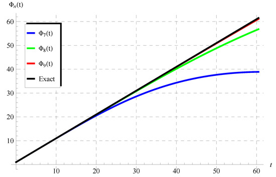
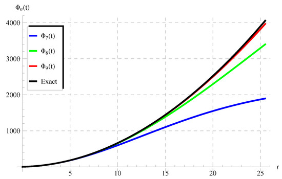
In the first case, we consider $c=-\frac{a}{b}$, and hence, the exact solution is available in Equation (60), given by

$$y\left(t\right)=\lambda \left[1+(a+b)t\right].$$

(68)

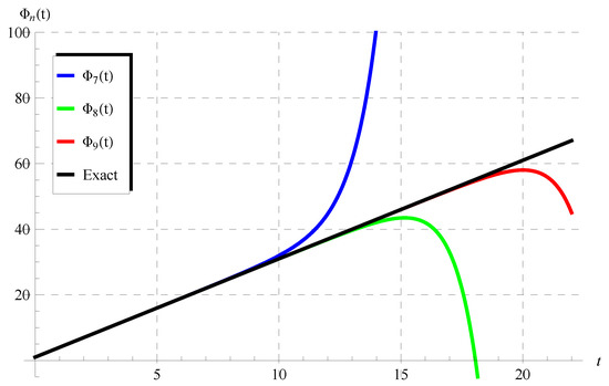
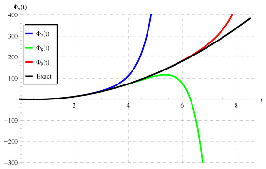
In Figure 1 and Figure 2, comparisons are performed between the approximations ${\Phi }_7\left(t\right)$, ${\Phi }_8\left(t\right)$, ${\Phi }_9\left(t\right)$ and the exact solution (68) when $a=-1$, $b=2$, $c=1/2$ (Figure 1) and $a=1$, $b=2$, $c=-1/2$ (Figure 2).

Figure 1. Comparisons between the approximate solutions ${\Phi }_n\left(t\right),n=7,8,9$ in Equation (67) and the exact solution in Equation (68) at $a=-1$, $b=2$, $c=1/2$.

Figure 2. Comparisons between the approximate solutions ${\Phi }_n\left(t\right),n=7,8,9$ in Equation (67) and the exact solution in Equation (68) at $a=1$, $b=2$, $c=-1/2$.

It can be seen from these figures that the approximation ${\Phi }_9\left(t\right)$ coincides with the exact solution in a wide range. However, such a domain of coincidence can be further enlarged by increasing the number of terms n taken in the EFS. To confirm this point, we consider an additional example for the case $c=\sqrt{-\frac{a}{b}}$ in which the exact solution is available in Equation (61), given by

$$y\left(t\right)=\lambda \left[1+(a+b)t+(a+b)\left(a+b{\left(-\frac{a}{b}\right)}^{\frac{1}{2}}\right)\frac{t^2}{2!}\right].$$

(69)

The comparisons are depicted in Figure 3 and Figure 4 between the approximations ${\Phi }_7\left(t\right)$, ${\Phi }_8\left(t\right)$, ${\Phi }_9\left(t\right)$ and the exact solution (69) at $a=-2$, $b=8$, $c=1/2$ (Figure 3) and $a=2$, $b=-8$, $c=1/2$ (Figure 4). It is also observed from these figures that ${\Phi }_9\left(t\right)$ is also close to the exact solution.

Figure 3. Comparisons between the approximate solutions ${\Phi }_n\left(t\right),n=7,8,9$ in Equation (67) and the exact solution in Equation (69) at $a=-2$, $b=8$, $c=1/2$.

Figure 4. Comparisons between the approximate solutions ${\Phi }_n\left(t\right),n=7,8,9$ in Equation (67) and the exact solution in Equation (69) at $a=2$, $b=-8$, $c=1/2$.

10. Conclusions

In this paper, two different canonical forms of the ADM were applied to solve the PDDE. The present approach lead to two types of closed-form solutions by which the PSS and the EFS were established. The solutions in the literature [12,15] were recovered as special cases of the obtained PSS for the ADDE. Several exact solutions were derived from the present PSS. The EFS was given in a closed form and compared with several exact solutions, which were determined from the PSS. Therefore, the advantages of the present method are explained in detail in the discussion section and also through the paper. Moreover, the obtained results reflect the efficiency and the effectiveness of the current approaches. Finally, the present method may deserve further extension to include a generalized class of delay differential equations such as $y^{\prime }\left(t\right)=ay\left(t\right)+by(ct-\tau )$.

References

- Available online: https://en.wikipedia.org/wiki/Pantograph (accessed on 9 November 2022).
- Andrews, H.I. Third paper: Calculating the behaviour of an overhead catenary system for rail-way electrification. Proc. Inst. Mech. Eng. 1964, 179, 809–846. [Google Scholar] [CrossRef] [Scilit]
- Abbott, M.R. Numerical method for calculating the dynamic behaviour of a trolley wire over-head contact system for electric railways. Comput. J. 1970, 13, 363–368. [Google Scholar] [CrossRef] [Scilit]
- Gilbert, G.; Davtcs, H.E.H. Pantograph motion on a nearly uniform railway overhead line. Proc. Inst. Electr. Eng. 1966, 113, 485–492. [Google Scholar] [CrossRef] [Scilit]
- Caine, P.M.; Scott, P.R. Single-wire railway overhead system. Proc. Inst. Electr. Eng. 1969, 116, 1217–1221. [Google Scholar] [CrossRef] [Scilit]
- Ockendon, J.; Tayler, A.B. The dynamics of a current collection system for an electric locomotive. Proc. R. Soc. Lond. A Math. Phys. Eng. Sci. 1971, 322, 447–468. [Google Scholar]
- Kato, T.; McLeod, J.B. The functional-differential equation y′(x) = ay(λx) + by(x). Bull. Am. Math. Soc. 1971, 77, 891–935. [Google Scholar]
- Iserles, A. On the generalized pantograph functional-differential equation. Eur. J. Appl. Math. 1993, 4, 1–38. [Google Scholar] [CrossRef] [Scilit]
- Derfel, G.; Iserles, A. The pantograph equation in the complex plane. J. Math. Anal. Appl. 1997, 213, 117–132. [Google Scholar] [CrossRef] [Scilit]
- Patade, J.; Bhalekar, S. Analytical Solution of Pantograph Equation with Incommensurate Delay. Phys. Sci. Rev. 2017, 2. [Google Scholar] [CrossRef] [Scilit]
- Fox, L.; Mayers, D.; Ockendon, J.R.; Tayler, A.B. On a functional differential equation. IMA J. Appl. Math. 1971, 8, 271–307. [Google Scholar] [CrossRef] [Scilit]
- Patade, J.; Bhalekar, S. On Analytical Solution of Ambartsumian Equation. Natl. Acad. Sci. Lett. 2017, 40, 291–293. [Google Scholar] [CrossRef] [Scilit]
- Alharbi, F.M.; Ebaid, A. New Analytic Solution for Ambartsumian Equation. J. Math. Syst. Sci. 2018, 8, 182–186. [Google Scholar] [CrossRef] [Scilit]
- Bakodah, H.O.; Ebaid, A. Exact solution of Ambartsumian delay differential equation and comparison with Daftardar-Gejji and Jafari approximate method. Mathematics 2018, 6, 331. [Google Scholar] [CrossRef] [Scilit]
- Alatawi, N.O.; Ebaid, A. Solving a delay differential equation by two direct approaches. J. Math. Syst. Sci. 2019, 9, 54–56. [Google Scholar] [CrossRef] [Scilit]
- Ebaid, A.; Al-Enazi, A.; Albalawi, B.Z.; Aljoufi, M.D. Accurate Approximate Solution of Am-bartsumian Delay Differential Equation via Decomposition Method. Math. Comput. Appl. 2019, 24, 7. [Google Scholar]
- Alatawi, A.A.; Aljoufi, M.; Alharbi, F.M.; Ebaid, A. Investigation of the Surface Brightness Model in the Milky Way via Homotopy Perturbation Method. J. Appl. Math. Phys. 2020, 8, 434–442. [Google Scholar] [CrossRef]
- Algehyne, E.A.; El-Zahar, E.R.; Alharbi, F.M.; Ebaid, A. Development of analytical solution for a generalized Ambartsumian equation. AIMS Math. 2019, 5, 249–258. [Google Scholar] [CrossRef] [Scilit]
- Khaled, S.M.; El-Zahar, E.R.; Ebaid, A. Solution of Ambartsumian delay differential equation with conformable derivative. Mathematics 2019, 7, 425. [Google Scholar] [CrossRef] [Scilit]
- Kumar, D.; Singh, J.; Baleanu, D.; Rathore, S. Analysis of a fractional model of the Ambartsumian equation. Eur. Phys. J. Plus 2018, 133, 133–259. [Google Scholar] [CrossRef] [Scilit]
- Ebaid, A.; Cattani, C.; Juhani, A.S.A.; El-Zahar, E.R. A novel exact solution for the fractional Ambartsumian equation. Adv. Differ. Equ. 2021, 2021, 88. [Google Scholar] [CrossRef] [Scilit]
- Ebaid, A.; Al-Jeaid, H.K. On the exact solution of the functional differential equation y′(t) = ay(t) + by(−t). Adv. Differ. Equ. Control Process. 2022, 26, 39–49. [Google Scholar] [CrossRef] [Scilit]
- Adomian, G. Solving Frontier Problems of Physics: The Decomposition Method; Kluwer Acad: Boston, MA, USA, 1994. [Google Scholar]
- Wazwaz, A.M. Adomian decomposition method for a reliable treatment of the Bratu-type equations. Appl. Math. Comput. 2005, 166, 652–663. [Google Scholar] [CrossRef] [Scilit]
- Ebaid, A. Approximate analytical solution of a nonlinear boundary value problem and its appli-cation in fluid mechanics. Z. Naturforschung A 2011, 66, 423–426. [Google Scholar] [CrossRef] [Scilit]
- Duan, J.S.; Rach, R. A new modification of the Adomian decomposition method for solving boundary value problems for higher order nonlinear differential equations. Appl. Math. Comput. 2011, 218, 4090–4118. [Google Scholar] [CrossRef] [Scilit]
- Ebaid, A. A new analytical and numerical treatment for singular two-point boundary value problems via the Adomian decomposition method. J. Comput. Appl. Math. 2011, 235, 1914–1924. [Google Scholar]
- Ali, E.H.; Ebaid, A.; Rach, R. Advances in the Adomian decomposition method for solving two-point nonlinear boundary value problems with Neumann boundary conditions. Comput. Math. Appl. 2012, 63, 1056–1065. [Google Scholar] [CrossRef] [Scilit]
- Chun, C.; Ebaid, A.; Lee, M.; Aly, E.H. An approach for solving singular two point boundary value problems: Analytical and numerical treatment. ANZIAM J. 2012, 53, 21–43. [Google Scholar] [CrossRef] [Scilit]
- Ebaid, A.; Aljoufi, M.D.; Wazwaz, A.-M. An advanced study on the solution of nanofluid flow problems via Adomian’s method. Appl. Math. Lett. 2015, 46, 117–122. [Google Scholar] [CrossRef] [Scilit]
- Bhalekar, S.; Patade, J. An analytical solution of fishers equation using decomposition Method. Am. J. Comput. Appl. Math. 2016, 6, 123–127. [Google Scholar]
- Diblík, J.; Kúdelcíková, M. Two classes of positive solutions of first order func-tional differential equations of delayed type. Nonlinear Anal. 2012, 75, 4807–4820. [Google Scholar] [CrossRef] [Scilit]
- Abbaoui, K.; Cherruault, Y. Convergence of Adomian’s method applied to nonlinear equations. Math. Comput. Model. 1994, 20, 69–73. [Google Scholar] [CrossRef] [Scilit]
- Cherruault, Y.; Adomian, G. Decomposition Methods: A new proof of convergence. Math. Comput. Model. 1993, 18, 103–106. [Google Scholar] [CrossRef] [Scilit]
- Alshaery, A.; Ebaid, A. Accurate analytical periodic solution of the elliptical Kepler equation using the Adomian decomposition method. Acta Astronaut. 2017, 140, 27–33. [Google Scholar] [CrossRef] [Scilit]
- Bakodah, H.O.; Ebaid, A. The Adomian decomposition method for the slip flow and heat transfer of nanofluids over a stretching/shrinking sheet. Rom. Rep. Phys. 2018, 70, 115. [Google Scholar]
- Li, W.; Pang, Y. Application of Adomian decomposition method to nonlinear systems. Adv. Differ. Equ. 2020, 2020, 67. [Google Scholar] [CrossRef] [Scilit]
- Ashpazzadeh, E.; Chu, Y.-M.; Hashemi, M.S.; Moharrami, M.; Inc, M. Hermite multiwavelets representation for the sparse solution of nonlinear Abel’s integral equation. Appl. Math. Comput. 2022, 427, 127171. [Google Scholar] [CrossRef] [Scilit]
- Hashemi, M.S.; Atangana, A.; Hajikhah, S. Solving fractional pantograph delay equations by an effective computational method. Math. Comput. Simul. 2020, 177, 295–305. [Google Scholar] [CrossRef] [Scilit]
- Hashemi, M.S.; Abbasbandy, S. A Geometric Approach for Solving Troesch’s Problem. Bull. Malays. Math. Sci. Soc. 2017, 40, 97–116. [Google Scholar] [CrossRef] [Scilit]
- Thabet, S.T.M.; Etemad, S.; Rezapour, S. On a coupled Caputo conformable sys-tem of pantograph problems. Turk. J. Math. 2021, 45, 496–519. [Google Scholar] [CrossRef] [Scilit]
- Thabet, S.T.M.; Etemad, S.; Rezapour, S. On a new structure of the pantograph inclusion prob-lem in the Caputo conformable setting. Bound. Value Probl. 2020, 2020, 171. [Google Scholar] [CrossRef] [Scilit]
- Ambartsumian, V.A. On the fluctuation of the brightness of the milky way. Dokl. Akad Nauk. USSR 1994, 44, 223–226. [Google Scholar]
Publisher’s Note: MDPI stays neutral with regard to jurisdictional claims in published maps and institutional affiliations. |
© 2022 by the authors. Licensee MDPI, Basel, Switzerland. This article is an open access article distributed under the terms and conditions of the Creative Commons Attribution (CC BY) license (https://creativecommons.org/licenses/by/4.0/).