Article

On Methods for Merging Mixture Model Components Suitable for Unsupervised Image Segmentation Tasks

Faculty of Mechanical Engineering, University of Ljubljana, Aškerčeva Ulica 6, 1000 Ljubljana, Slovenia
*
Author to whom correspondence should be addressed.
Mathematics 2022, 10(22), 4301; https://doi.org/10.3390/math10224301
Submission received: 11 October 2022 / Revised: 3 November 2022 / Accepted: 14 November 2022 / Published: 16 November 2022

Abstract

:
Unsupervised image segmentation is one of the most important and fundamental tasks in many computer vision systems. Mixture model is a compelling framework for unsupervised image segmentation. A segmented image is obtained by clustering the pixel color values of the image with an estimated mixture model. Problems arise when the selected optimal mixture model contains a large number of mixture components. Then, multiple components of the estimated mixture model are better suited to describe individual segments of the image. We investigate methods for merging the components of the mixture model and their usefulness for unsupervised image segmentation. We define a simple heuristic for optimal segmentation with merging of the components of the mixture model. The experiments were performed with gray-scale and color images. The reported results and the performed comparisons with popular clustering approaches show clear benefits of merging components of the mixture model for unsupervised image segmentation.
MSC:
68U10; 94A08; 62H35; 68T45

1. Introduction and Background

Intelligent computer vision systems are becoming increasingly popular. They are very useful tool in many applications that aid the decision making process, for example, agriculture [1], structural health monitoring [2], robotics [3], surveillance [4], product quality and manufacturing [5], self-driving-vehicles [6], medicine [7], and so on.
Image segmentation can be viewed as a useful partitioning of the image. As such, it is a central task in many computer vision systems, and one of most difficult ones [8,9,10,11]. It can be supervised or unsupervised, as pointed out by Refs. [12,13]. In supervised image segmentation, we want to partition the image into semantically coherent regions on the image. This can also be referred to as semantic segmentation [3,14]. As such, it is usually based on classification methods [13,15,16]. In unsupervised image segmentation, we are interested in extracting similar segments based on pixel positions and color intensity values with respect to a criterion [17]. As such, clustering algorithms are mostly used [11,12,17,18].
For supervised image segmentation, we usually need very large datasets for training a classification model, e.g., a deep neural network [2,14]. In unsupervised image segmentation, we perform a clustering algorithm directly on the image under consideration [12,17]. Consequently, unsupervised image segmentation based on a clustering algorithm is weaker in performance than classification. However, they do not require large training datasets, are faster, require less computational power, and, most importantly, can be used in conjunction with newer classification methods [3,12,13]. They are also much more useful than their supervised counterparts for certain domain-specific tasks where prior knowledge is lacking, whether due to a lack of plausible training images or other factors [12,13,19,20].
A mixture model is a compelling framework for many pattern recognition tasks [21,22,23,24]. Traditionally, it is used in machine learning as a clustering tool and, therefore, in computer vision for unsupervised image segmentation [22,25,26,27]. Mixture models can be seen as blob detectors, aimed at detecting regions of interest with similar colors or intensities in an image [9,25,28]. In this respect, similar to the fuzzy clustering algorithms [10,12,29], they are very promising for unsupervised image segmentation and as such can be useful for further feature extraction and detection of region of interests [8,19].
Obtaining a useful segmentation with the mixture models is a delicate process. First, the right mixture model must be chosen, i.e., Gaussian, Gamma, Weibul, or another that can capture the detail correctly [11,25,30,31]. Next is the choice of model selection criterion [32]. Finally, the algorithm for estimation can be problematic [9]. All of the above-mentioned can result in either under-segmentation problems (too few regions detected) or over-segmentation (too many segments detected) [9,28,33]. An over-segmented image can be regarded as noisy, while an under-segmented image as incomplete and thus inappropriate for use. To tackle this issue, in this paper, we investigate the usefulness of a clearly over-segmented solution, provided by the estimated mixture model, and the methods for merging different detected regions to obtain a more useful segmentation.
Every component of the estimated mixture model represents a segment of the image, in order to reduce the number of unwanted segments. We are interested in merging different components of the mixture model [33]. By doing so, we are remedying the problems that arose as a result of an inappropriate type of mixture model, the deficiency of model selection criteria, and, to some extent, drawbacks of the estimation algorithm [33,34,35]. We are investigating if many-to-one mapping as a one-to-one relationship between a mixture model component and a cluster may be insufficient [9,33].
This paper is summarized as follows. We start with an explanation of mixture models and their application in clustering and image segmentation in Section 2. Section 3 is reserved for the derivation of merging procedures and criteria for merging. Section 4 describes the estimation algorithm. Section 5 discuses the optimal segmentation. Section 6 introduces the needed constants for evaluation and in Section 7 we provide the experimental results. In Section 8 we provide some fruitful discussions of the experimental results, and Section 9 finalizes our work and concludes this paper.

2. Mixture Models

Let Y = { y 1 , y 2 , , y n } be a d-dimensional observed dataset of n continuous observations y j = { y 1 , y 2 , , y d } . Each observation y j is assumed to follow the probability density function (PDF):
f ( y j | c , w , Θ ) = l = 1 c w l f l ( y j | Θ l ) .
Equation (1) gives the PDF of a mixture model. The PDF of a mixture model consists of weighted c components that follow simple parametric probability distribution, such as Gaussian distribution, Weibull distribution, and similar [36,37]. Component distribution PDF is given by the f l and has the parameters Θ l . For example, PDF of multivariate Gaussian distribution is
f l ( y j | Θ l ) = 1 ( 2 π ) d det ( Σ l ) exp 1 2 ( y j μ l . ) Σ l 1 ( y j μ l ) T .
Component parameters Θ l are distribution specific. For the Gaussian mixtures, those are the mean vector μ l and covariance matrix Σ l . Weights w l have the properties of the convex combination w l 0 l = 1 c w l = 1 [38]. Thus, we can arrange the mixture model parameters in a set Θ
Θ = { w 1 , w 2 , , w c , Θ 1 , Θ 2 , , Θ c } ,
or concisely and more conveniently
Θ = { w , Θ } .
The estimation of the parameters involves estimation of component weights w and component parameters Θ . Usually, we denote the estimations as Θ ^ . The easiest way to estimate the mixture model parameters is via the maximum likelihood. In other words, the parameters Θ ^ yielding the maximum of
L ( Y | Θ = Θ ^ ) = j = 1 n f ( y j | c ^ , w ^ , Θ ^ ) .
It is often more convenient to maximize the log-likelihood function
log L ( Y | Θ ) = j = 1 n log l = 1 c w l f l ( y j | Θ l ) ,
and, the estimation can be written as
Θ ^ = argmax Θ log L ( Y | Θ ) .
The maximization problem described with Equation (7) has many inconvenient aspects, mainly because the number of components c in the mixture model is not known in advance. First, it is known that the likelihood value increases with the increase in the number of components due to the overall better fit [28,39]. Second, without knowing the number of components, it is impossible to derive the (6) to obtain the solution to the maximization problem. Lastly, the use of global optimization algorithm is not convenient due to the large number of optimization parameters involved in a mixture model [38]. Thus, some type of model selection procedure is commonly involved in the estimation process [38].

2.1. Model Selection

Usually, we are interested in estimating the number of components c ^ and the accompanying parameters Θ ^ ; however, in some cases, the number of components is known [38], in which case the model selection procedure is not needed—this occurs in the minority of cases. In the majority of cases, we are faced with a ubiquitous problem of the maximization of (6) when the number of components is unknown. Nonetheless, to derive Equation (6), we need to know the number of components c. Therefore, it is a common practice to try out different numbers of components and estimate the fit. Thus, it is quite common and justified to denote the mixture model in relation to the number of components c,
Θ ( c ) = { w ( c ) , Θ ( c ) } .
Additionally, because the likelihood function increases with the increase in the number of components, the selection of the optimal model based solely on maximum likelihood can be misleading. Therefore, there is a need to introduce different model criteria to choose the best fit. Generally, those are called information criteria [38]. We will denote those as I C . The model selection procedure is described with Algorithm 1 [28,39].
In summary, we estimate the optimal mixture model Θ ^ for different numbers of components c. If the number of components is known, we can solve Equation (7) using, for example, the algorithm EM (expectation–maximization) denoted by the EM function in line 4 of the Algorithm 1. EM is a local optimization algorithm mainly used to estimate the maximum likelihood parameters of mixture models when some initial parameter estimates are known in advance [38]. The optimal model is obtained for each number of components, and the best model is selected from among them. The model giving the optimal selected I C opt is thus the best model available. ICF in line 5 of Algorithm 1 represents the generic function for estimating the chosen information criterion.
Algorithm 1: Model selection procedure
Input: dataset Y and initialize set C = { c 1 , c 2 , } ;
Output: optimal mixture model parameters w opt , Θ opt ;
  •     I C opt = , w opt = { } , Θ opt = { } , c opt = 0 ;
  •    foreach   c C do:
  •         Initialize w ini ( c ) , Θ ini n i ( c ) ;
  •          w ( c ) , Θ ( c ) = EM( Y , w ini ( c ) , Θ i n i ( c ) );
  •         Estimate criterion I C = ICF ( Y , w ( c ) , Θ ( c ) ) ;
  •         if  IC   <   I C opt :
  •              I C opt = I C , c opt = c , w opt = w ( c ) , Θ opt = Θ ( c ) ;
  •         end
  •    end
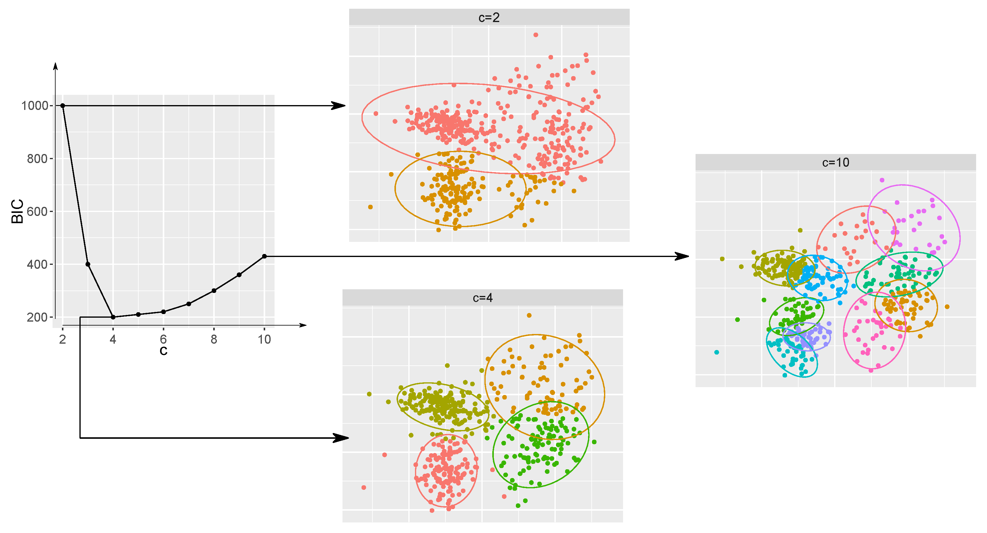
The importance of using a model selection procedure is illustrated in Figure 1. Different models were estimated for different numbers of components c. For each model, a Bayesian information criterion (BIC) was calculated [40]. The BIC is defined as
BIC = 2 log L + M log n ,
where M is the number of parameters in the model. It is quite obvious that the term M log n , given that the M increases with the number of components c, is a balance factor to compensate for the increase in log-likelihood value with the increase in number of components c.
BIC is also one of the most commonly used information criteria [41]. Choosing the model with the optimal value of BIC should provide the best solution [33,34]. Although every estimated model yields one of the local optima of log-likelihood function from (6), different models provide less or more of the information needed. For example, a model with two components clearly is an under-fit, while a model with ten components gives an over-fit. In contrast, a model with five components seems to be the best selection, at least when the BIC criterion is used.

2.2. Mixture Model-Based Clustering and Image Segmentation

In a mixture model framework, it is generally considered that each component in a model represents one homogeneous unit [42]. In other words, that homogeneous unit represents a sub-population of the whole population. In a clustering sense, that homogeneous unit represents the cluster. A cluster is a group of observations from a dataset that share similar characteristics. Thus, every observation that arose from a certain component in a mixture model is considered to form a cluster. For every observation y j in dataset Y , we can estimate the posterior probability
τ j l = w l f l ( y j | Θ l ) l ˜ = 1 c w l ˜ f l ˜ ( y j | Θ l ˜ ) ,
that it arose from the lth mixture model component. The cluster assignment is made according to the maximum a posteriori (MAP) rule
l j = argmax l ˜ = 1 , , c τ j l ˜ j { 1 , , n } .
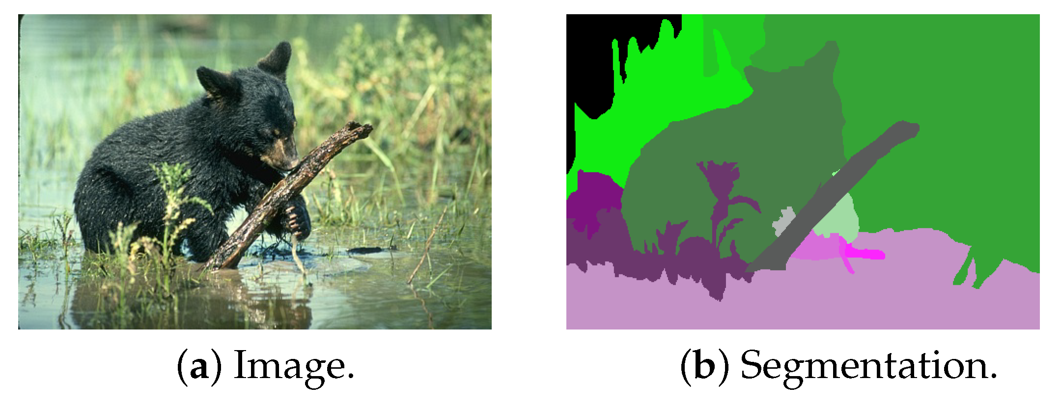
We are interested in labeling all of the observations in dataset Y : ergo, a clustering scheme or simply clustering. Image segmentation is a similar process. We want to identify k partitions of the image, which are coherent in some way. This is illustrated in Figure 2. The original image in Figure 2a comes from the Berkeley dataset [43] and the second image (Figure 2b) is the human segmentation provided by the participants in study.
Many clustering algorithms are used for image segmentation [44]. Image segmentation with a mixture model can be conducted using pixel intensity and position; however, using the pixel position values in the estimation of the mixture model often degrades the results, due to their non-random nature. Thus, we are interested only in modeling the PDF of pixel intensity; accordingly, we produce a clustering (scheme). Additionally, for the component distribution, the Gaussian distribution is usually used [9,31]. This is a popular choice because the multivariate extension is straightforward; thus, images with multiple channels (color images opposed to monochrome images) can be segmented. Furthermore, the mixtures of Gaussian distributions are the easiest and most straightforward to estimate. However, using Gaussian distribution as the component distribution brings many problems. The first is that the pixel intensity is bounded, while the Gaussian distribution is not. The second problem arises from the fact that the Gaussian PDF is symmetric around the mode. Because of the non-symetricity of the mode (i.e., the left and right tails are not equal), multiple Gaussian components are estimated to compensate for this. This leads to many clusters, which then leads to many segments, which are not actually present. Although these problems generally arise with the Gaussian mixture model, the problem of estimating too many components in other mixture models is also present, especially when estimating the PDF of an image.

3. Merging of Redundant Components in Mixture Model-Based Clustering

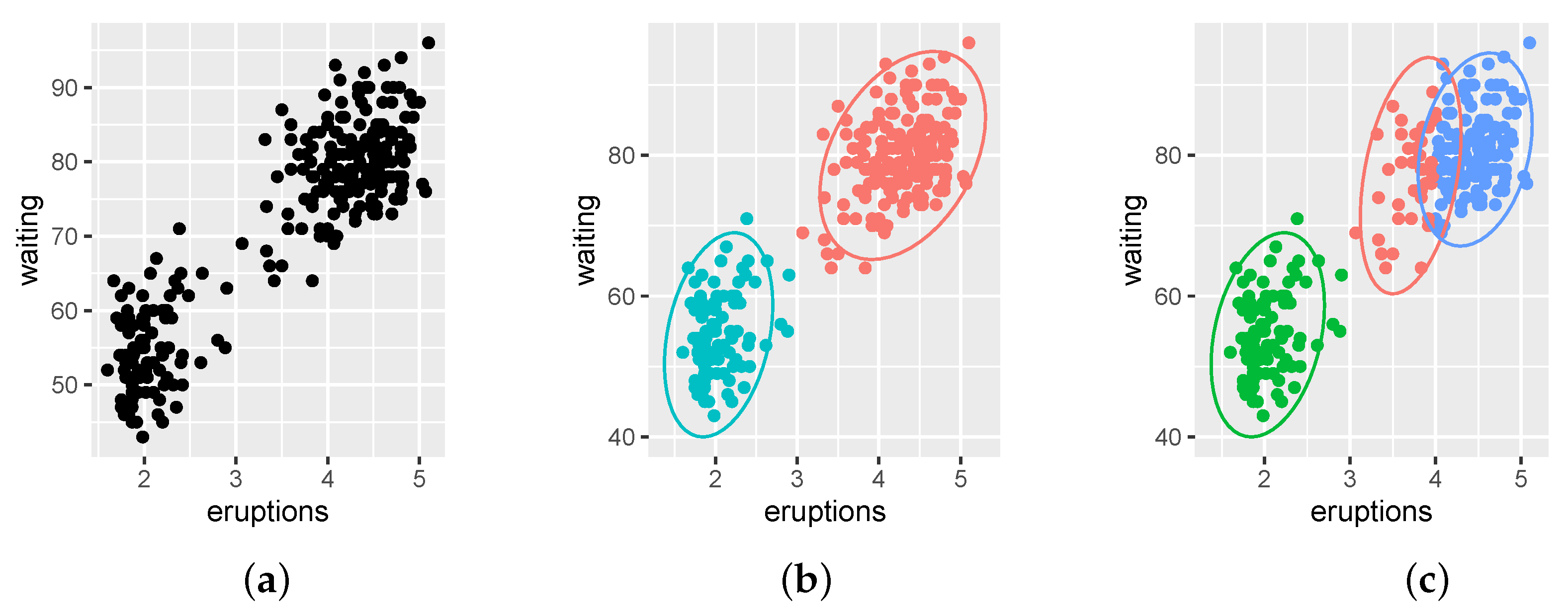
Let us look at the quite famous old faithful geyser dataset [45]. The dataset contains 272 observations on two continuous variables, the first named eruptions and the second named waiting, as illustrated on plots in Figure 3. The first variable, eruptions, gives the geyser eruption time in minutes, whilst the second one, waiting, gives the waiting time to next eruption, also in minutes. Figure 3a gives the visualization of the dataset without identified clusters while Figure 3b,c give the clustering solution obtained from the estimated two-component Gaussian mixture model and the three-component Gaussian mixture model.
It occurs quite naturally that the two-component clustering solution is true. Not even by looking at the solution on plot Figure 3b and only by observing non-colored points in plot Figure 3a there is some convincing evidence that there are two groups of points. However, let us examine the obtained values of the IC criteria in Table 1. Even though the difference in IC values is not so dramatic, the three-component solution is the optimal solution judging by two different IC, namely AIC (Akaike information criterion [46]) and BIC. Judging by their value, the three-component solution seems to be a preferred solution. In contrast, the ICL (integrated classification likelihood [42]) criterion had a lower value for the two-component mixture, meaning that this model would be selected as optimal. This is expected because the ICL criterion favors the solution that is more probable to be the optimal clustering solution. The sole reason for the derivation of the ICL criterion is to bypass the somewhat tricky nature of BIC to favor the model that is not an optimal clustering solution.

3.1. Entropy-Based Merging

While the ICL criterion seems to be sufficient for the old geyser dataset and gives an optimal clustering solution, it is far from bulletproof. Mainly, the problem is that it can provide a clustering solution with too few clusters in highly overlapping situations [34]. In image segmentation, such situations are frequent. Another point is provided in [34]. Although the number of components in the mixture model is well met by, e.g., the BIC criterion, the number of components in that scenario is well suited for the underlying PDF of a dataset but not necessarily for clustering. That may well mean that some clusters in the clustering are not well-presented with only one component of the mixture model, meaning that a one-to-one scenario is not practical. This goes hand in hand with many density-based clustering approaches, especially the likes of mean-shift or modal-based EM algorithm [47].
To propose a solution, Baudry et al. [34] developed a merging procedure based on the estimation of entropy of soft clustering: in other words, posterior probabilities. Starting with a number of components c in the mixture model that fits the dataset well and an equal number of clusters k = c as the number of components in the mixture model, the idea is to build a sequence of clusterings with merged pairs of clusters. Thus, the newly created clustering schemes contain k 1 clusters. At each stage, merging happens between each and every pair of clusters and the most promising pair for creating the k 1 clustering scheme is the one for which the newly obtained k 1 clustering scheme maximizes a criterion
E l l ˜ = j = 1 n τ j l log τ j l + τ j l ˜ log τ j l ˜ + j = 1 n τ j l l ˜ log τ j l l ˜ ,
where the τ j l gives the posterior that the j th observation belongs to lth component/cluster, τ j l ˜ gives the posterior that the j th observation belongs to l ˜ th component/cluster, and the τ j l l ˜ is the posterior of the merged cluster combined from components/clusters l and l ˜ . The posterior τ j l l ˜ can be simply calculated as
τ j l l ˜ = τ j l + τ j l ˜ ,
and obvious condition l l ˜ should be met. The number of combinations is therefore equal to
k 2 = k ! 2 ( k 2 ) ! = k ( k 1 ) 2 ,
when the current number of components/clusters is k.
The final selected merged clustering scheme fits the data as well as the first solution provided by the c mixture model components, since it is based on the same mixture model and the likelihood does not change. Only the number and definition of clusters are different. In contrast, the likelihood of the mixture model selected by the ICL criterion can be worse. The method described above yields just one suggested set of clusters for each k, and the user can choose between them on substantive grounds. For example, the number of clusters in the final clustering scheme can be selected to match the number of components in the mixture model selected with the ICL criterion. Otherwise, because in each merging step we obtain the entropy of merged pair of clusters from the previous clustering scheme, the elbow method can be employed on graphical results of the entropy variation against the number of clusters to select the final number of clusters k [34].

3.2. Merging Based on Directly Estimated Mis-Classification Probabilities

The second method is described by [35]. As the previous method described, this method depends on soft clustering or, in other words, posterior probabilities τ l j and hard clustering or indicator value 1 l j . Indicator value 1 l j is a binary variable giving the indicator if the observation y j belongs to lth component/cluster. However, we are not interested in the probability of observation being clustered to the lth component/cluster but the misclassification probability between two components of the mixture model p l l ˜ . The misclassification probability p l l ˜ can be summarized as the distance between two probability distributions, e.g., for two Gaussian distributions, a Bhattacharyya distance [35], but in a more generalized fashion and additionally more focused on clustering application. The misclassification probability can be estimated as
p ^ l l ˜ = j = 1 n τ l j 1 ( l ˜ j ) j = 1 n τ l j ,
where the τ l j is the soft clustering for the lth component/cluster and 1 ( l ˜ j ) is the hard clustering for the l ˜ th component. It is also important to say that the p ^ l l ˜ is not symmetric, meaning that p ^ l l ˜ p ^ l ˜ l ; however, this can be violated. Thus, the most optimistic criterion is the
q = max p ^ l l ˜ , p ^ l ˜ l ,
and should be used to select the merging pair of components/clusters. Again, it is quite obvious that the merged pair will result in equal posterior probabilities τ j l l ˜ as for the previous described method (Equation (13)).
Merely by observing the merging criteria in both methods, it is sufficient to say that both procedures will results in different final clustering schemes. Nonetheless, they share several similarities, given that the l = 1 k τ l j = 1 must hold for any number of clusters k c . The most important similarity, at least for the image segmentation task, is the obvious merging of overlapping components. Namely, two components, not overlapped significantly, will obey the rule of τ l j > > τ l ˜ j j { 1 , , n } or vice versa. In other words, one component will have posterior probabilities close to 1, while the other will have close to 0. Thus, both criteria (Equations (12) and (16)) will be close to 0, suggesting the component should not be merged. Otherwise, if the significant overlap between components exists, both criteria will yield significantly higher values, suggesting that the components should be merged. Simply, the methods will progress to the solution that will minimize the overlap between the posterior probabilities. If the overlap between the mixture model components is not high both methods will yield similar solutions; however, in the presence of high overlap between the components of the mixture model, both methods will give different results.

3.3. Component Merging Mechanism Inside Mixture Model

An advantage of both selected merging methods and criteria is in the fact that they can be used for any component distribution in the mixture model, as they both are distribution parameter independent [35]. Instead of recalculating the best possible merging pair based on distribution component parameters, we are calculating the best possible merging pair based on posterior probabilities τ l j and clustering labels (indicator values) 1 l j . Thus, both methods have a wider range of application. Furthermore, instead of recalculating new component parameters for new merged pairs, we simply store the merging tree, and only update the posterior probabilities with Equation (13) to reflect the current/desirable number of clusters. Cluster indicator values for new merged clusters can be obtained merely by summing the indicator values of previously merged pair of clusters:
1 j l l ˜ = 1 j l + 1 j l ˜ ,
and cluster labels by the union of cluster labels of cluster pairs to be merged. Essentially, we are performing a form of hierarchical clustering on mixture model components. By doing so, we maintain the flexibility of a merged cluster being defined by multiple mixture model components.

4. REBMIX Algorithm and Connection with Image Segmentation

This section develops the connection of the REBMIX (Rough-Enhanced-Bayes mixture estimation) algorithm and its usefulness in image segmentation. We will not cover details about the REBMIX algorithm already described in many papers [24,36,37,48,49]. As already indicated by [28], the REBMIX algorithm is a heuristic useful for the estimation of mixture model parameters based on empirical density estimation. The first step in the multi-step procedure employed is the pre-processing step in which the empirical density estimation is carried out. This empirical density estimate can be made with different techniques; however, we are interested in the histogram, which is, in essence, how the pixel density values in an image can be naturally compressed. Given that the digital images are represented by single (gray scale) or multiple channels (color, RGB or otherwise), which are vectors of integers, the input parameter for the REBMIX algorithm pre-processing step is known in advance. For the different bit depths of digital image, this parameter varies; e.g., for 4-bit images this parameter is K = 2 4 = 16 and for the 8-bit it is K = 2 8 = 256 and so on. Given that the 8-bit digital images are predominantly used, K = 256 can be adopted most of the time, because the pixel intensity is an integer value between 0 and 255. However, as pointed out in [28], this parameter can lead to the overflowing of estimated mixture model components, which again emphasizes the merging of components in the mixture model.

5. Optimal Image Segmentation

In revising the merging criteria, we have already given some of the heuristics mentioned in [34,35] that indicate when is optimal to stop merging the mixture components and yield final clustering solution. We will revise them here and propose some more practical ones, especially with respect to image segmentation. As mentioned before, one could aim that the final number of clusters after merging is equal to the number of components of the mixture model selected with the ICL criterion. On the other hand, the merging process could be stopped if the merging criterion is lower than a predetermined lower bound for that specific merging criterion. For example, [35] gives the lower bound for the DEMP merging criterion q * = 0.05 in his experiments. The introduction of new hyperparameters seems, at least to us, somewhat problematic. They might work in one situation and not in another. Their values vary considerably for different examples, leaving a lot of leeway to the user. This can be encouraging and annoying at the same time. We would like to avoid this. In addition, they are usually difficult to automate. The best we can do is to use the elbow method to determine the optimal value. In other words, the heuristic here is the knee of a curve obtained by plotting the values of the merging criterion and the number of clusters. In clustering, we justify this with the notion of loss of explanation due to subsequent merging. We further note that using the elbow method for our purposes leads to the following problem. The digitized nature of the image intensities may result in multiple elbows (or knees), leading to multiple plausible stops, making this heuristic unappealing. Finally, we may also want to use a different metric that does not depend on the mixture model and is more focused on the current application, namely image segmentation.
Measuring entropy has proven to be a useful metric in many artificial intelligence image applications [50,51,52,53]. The entropy of an image is simply defined as
H = j p j log p j ,
where j is the unique color in the image and p j is the probability of its occurrence. Segmenting the image using the mixture model with c components yields the entropy estimate
H = l = 1 c w l log w l .
It is trivial to see that subsequently merging the mixture components reduces the estimated entropy, since H ^ 0 when c 1 due to the property of mixture components weights is l = 1 c w l = 1 . Therefore, to approach a practical solution, we propose an average of the image segmentation entropy of the form
E ( H ) = l = 1 c w l 2 log w l .
Finally, it should be noted that this average of the image segmentation entropy is in no way related to the average entropy of [54], where the goal is the average entropy estimate of a continuous random variable. The optimal image segmentation can therefore be chosen to maximize the average of the image segmentation entropy or max E ( H ) .

6. Experimental Setup

In this section, we further describe the experiments, experimental algorithm settings, different algorithms used, and metrics used for the results evaluation. Experiments are conducted on digital images. Digital images can have multiple channels. Usually, color digital images have three or more channels. Each channel represents one of the primary colors and its intensity. However, monochrome digital images (gray-scale) have only one channel, which contains only the amount of light, i.e., the intensity.
Color digital images carry much more information; thus, they are more demanding for processing. In contrast, monochrome images are easier to process, as they have less information. Some algorithms used for image processing are also only capable of processing gray-scale images. Therefore, color images need to be transformed into gray-scale. A mixture model-based approach is capable of handling color images and, therefore, also gray-scale images. Because gray-scale processing requires fewer parameters to be estimated, it has a better prognosis on gray-scale images. Nonetheless, the results for color images can be promising, as seen in [28].
Thus, the mixture model approach for clustering to both gray-scale and color images will be used to obtain segmentation. For the mixture model, we will use the Gaussian mixture model. For the information criterion, we will use BIC; for the model selection estimation strategy, we will use single REBMX and EM from rebmix R package. The strategy is fully described in [39]. In essence, we are combining both REBMIX and EM algorithms to obtain the best possible estimations while keeping the computation overhead minimal, by providing the smoothing parameter K to the REBMIX pre-processing step. The value of parameter K = 256 is described in the previous section. The maximum number components to consider in model selection procedure is c max = 15 . The merging of mixture model components with the entropy criterion, explained in Section 3.1, is referred to as ENT, and the merging of mixture model components with directly estimated misclassification probabilities, explained in Section 3.2, is referred to as DEMP. In addition, a single REBMX and EM strategy with ICL criterion is used as a baseline approach for optimal image segmentation with Gaussian mixture models. We refer to this as ICL.
We will use several useful external clustering metrics to quantitatively evaluate various image segmentation results.
 Remark 1. 
For completeness, we reiterate that the terms segmentation and clustering are used interchangeably, as they are equivalent in this context and refer to the same thing. For aesthetic reasons, we use the term segmentation when we want to emphasize the clustering application of image partitioning.
We use precision P, recall R, Dice score F 1 , Jaccard score, adjusted rand index A R I , and adjusted mutual information A M I . Precision and recall are self-explanatory. The former is the frequency of correctly predicted positives among all predicted positives and the latter is the frequency of correctly predicted positives among all correctly predicted positives. The Dice score is the harmonic mean between Precision and Recall, and the Jaccard score or better known as Intersection over Union is the frequency of correctly predicted positives among all true positives and predicted positives. Formally we define them with following equations
P = T P T P + F P
R = T P T P + F N
F 1 = 2 · T P 2 · T P + F P + F N
F = T P T P + F P + F N
where in clustering
  • True positives ( T P ) is the number of pairs of points belonging to the same cluster in predicted and true clustering;
  • False positives ( F P ) is the number of pairs of points belonging to the same cluster in true clustering but they are in different clusters in predicted clustering;
  • False negatives ( F N ) is the number of pairs of points belonging to the same cluster in predicted clustering but they are in different clusters in true clustering;
  • True negatives ( T N ) is the number of pairs of points that do not belong to the same cluster in predicted and true clustering.
These four metrics give several meaningful aspects of segmentation quality with different clustering algorithms compared to ground truth (i.e., perfect or true segmentation). On the other hand, we use A R I and A M I to provide a measure of agreement between two clustering solutions, i.e., predicted and true clustering, that takes into account the randomness of cluster assignments. This is especially important when the number of clusters in the predicted and true clustering is different and when the number of predicted clusters is large. A R I is defined in the range 1 , 1 , with values less than 0 indicate that clustering is worse than performing clustering at random, while values greater than zero generally define the degree of agreement between clusters. A M I is defined in the range 0 , 1 , with values closer to 0 indicating largely independent clusters between the predicted and true clustering, and values closer to 1 indicating stronger agreement between clusters in the predicted and true clustering. The equations for A R I and A M I are somewhat unwieldy, and to avoid further repetition and unnecessary lengthening of the text, we omit them here. Interested readers may wish to consult them in [55], for example.
Finally, a note on clustering algorithms used alongside mixture modeling. There are many clustering algorithms, but the most popular ones, and thus the ones we use for comparison here, are discussed in more detail in the following two groups.
  • EM algorithm with Gaussian mixtures denoted as GMM [38], K-means denoted as KMEANS [56], and Fuzzy C-means denoted as FCMEANS [57],
  • and Meanshift denoted as MS [58], Density-based clustering denoted as DBSCAN [59], and Ordering Points To Identify the Clustering Structure denoted as OPTICS [60].
In the first group of clustering algorithms, the number of clusters must be determined in advance. We will use these algorithms for the experiments if we want to obtain the clustering solution with the desired number of clusters (segments). The second group of clustering algorithms estimates the optimal number of clusters based on internal criteria, providing the optimal clustering. We will use these algorithms for optimal segmentation of images. For their implementation, we use the scikit-learn library for the Python programming language [61]. To use them in the context of image segmentation, we followed the procedure of [44]. First, we used the SEEDS (Superpixels Extracted via Energy-Driven Sampling) superpixel algorithm [62] (from OpenCV library) and reduced the number of pixels in the image. In addition, we tried different values of the required parameters to obtain the best possible segmentation on several images. Once we were satisfied, we kept these values for further evaluation.

7. Experiments

In this section, we further report the results obtained by applying different clustering algorithms to digital images from different datasets. We use these for comparative studies of the discussed merging criteria and the optimal clustering obtained based on the heuristics we proposed in Section 5.

7.1. Crack Image Segmentation

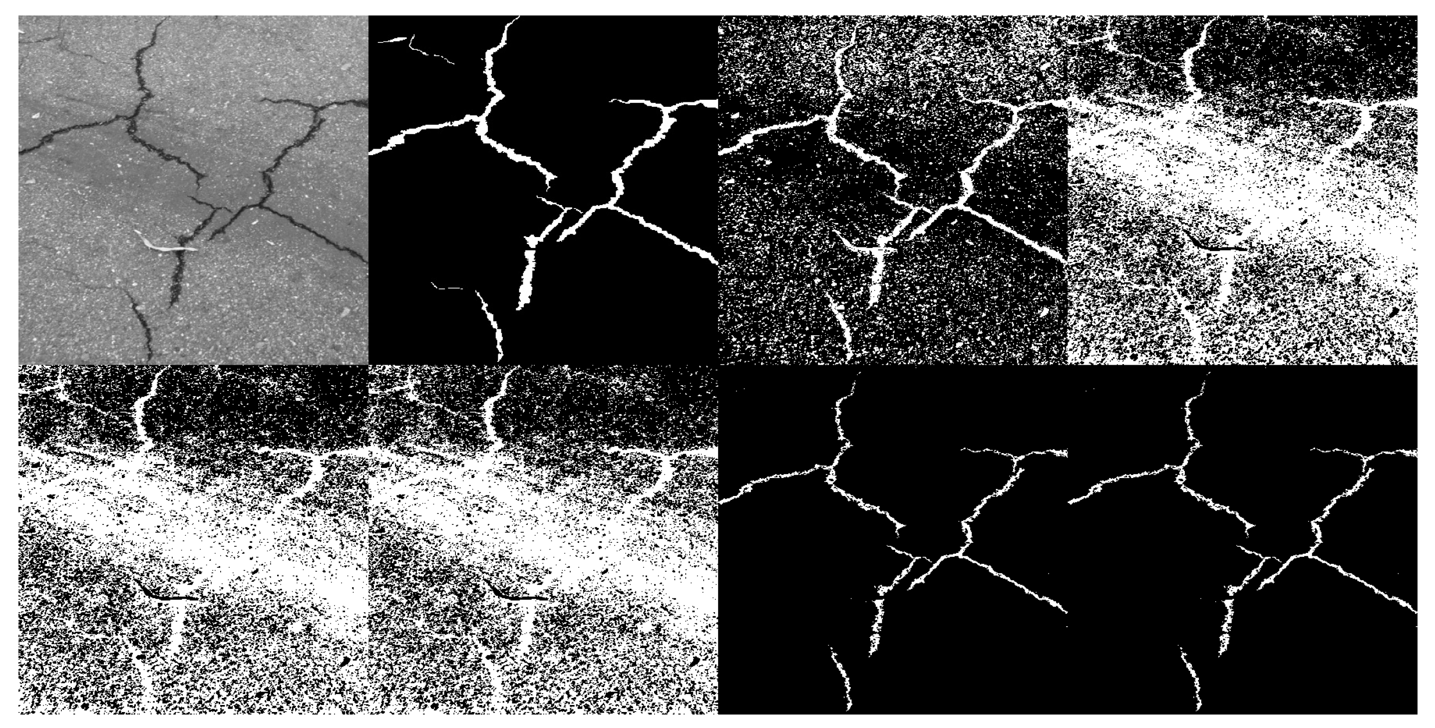
In the first experiment, we will investigate the usefulness of our proposal for the problem of segmenting crack images (see Figure 4). This is a widely known and studied problem in the literature [63]. The goal is to extract the pixels from the digital images that belong to the observed crack on the digital image, essentially a foreground/background segmentation. The images examined are monochromatic (gray-scale) because the crack on the image usually manifests as an area of lower intensity (darker). Many thresholding methods commonly used for this problem fail because the gray density distributions representing the background and foreground are not normal or appear as quasi-unimodal functions [64]. In addition to thresholding methods, a clustering approach is also useful. It can be considered as a two-cluster problem, but may fail because the background and/or foreground object are not optimally estimated with a single distribution and thus require subsequent merging.
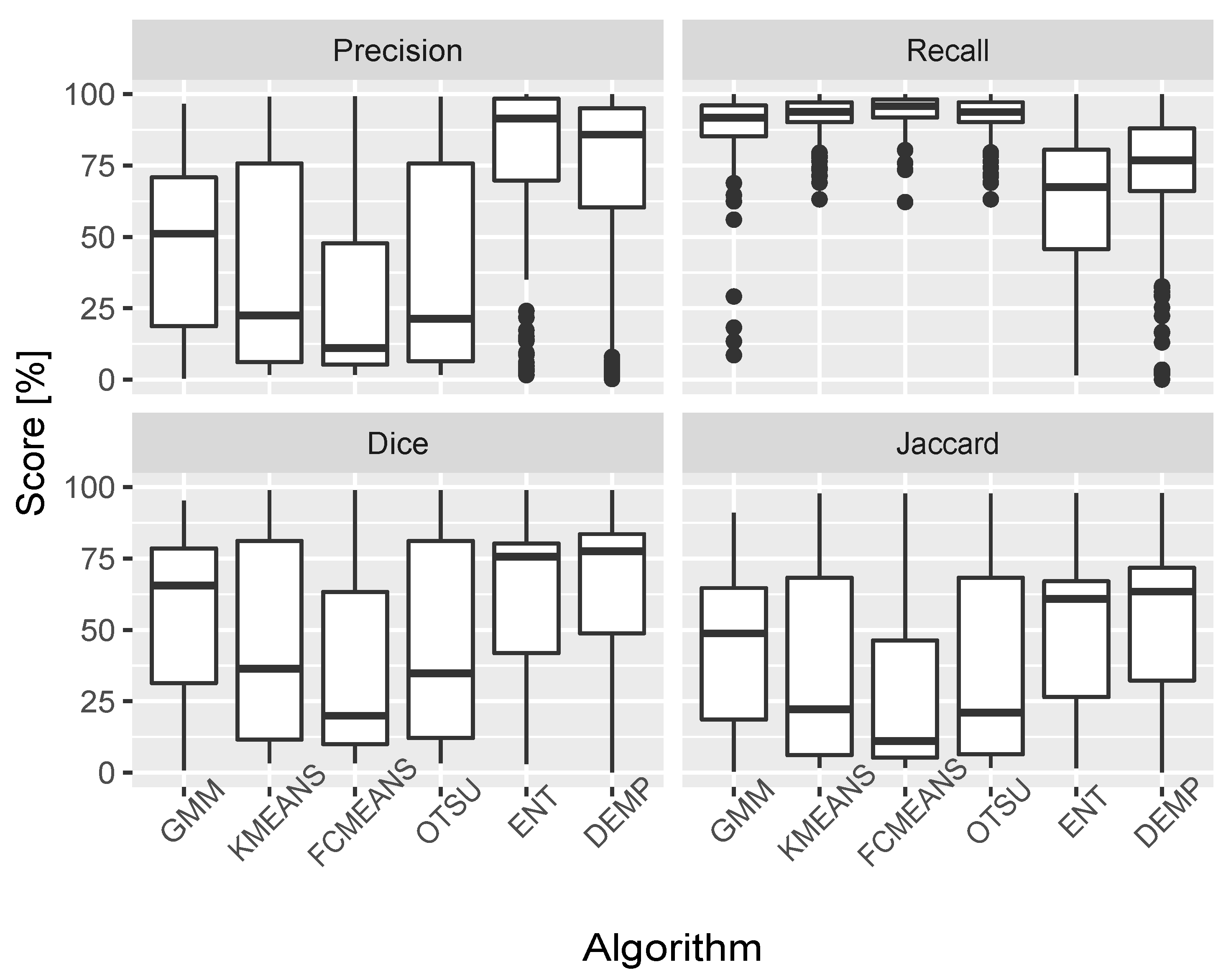
For this task, we examined 250 different images that can be found on online dataset repositories. Most of them are from previous studies of crack image segmentation, such as Ref. [63]. The qualitative results can be found in Figure 4. The quantitative results are presented in Figure 5 in the form of boxplots, and the summary average values of the four metrics studied can be found in Table 2. We chose to examine only Precision, Recall, Dice, and Jaccard score because we knew exactly how many segments the optimal segmentation should contain, namely two segments.
From the reported results, it is clear that merging the components with either ENT or DEMP criteria results in much better segmentation than the compared algorithms. For clarity, we have also included the famous Otsu thresholding method (OTSU), although it is not a clustering method. It is also worth noting that we are dealing with an unbalanced problem, which is why the recall value is slightly exaggerated. This is because the cracks only occupy a small portion of the image. Even if the returned segmentation contained only one segment (i.e., no crack was detected), the percentage of correctly returned pixels out of all positively returned segments is still high. On the other hand, the precision is low because the false-positive pixels may exceed the true-positive ones. Judging by the Dice and Jaccard score, the ENT and DEMP algorithms that use mixture merging are far superior.

7.2. Natural Image Segmentation

The second experiment is natural image segmentation. This is the most common application of image segmentation methods. The goal is to obtain a meaningful segmentation of the image that indicates the different coherent regions in the image. The first experiment is considered a simpler task, so we used only gray-scale variants of the images. The second experiment is much more challenging, as the variations of the different objects on the natural image are harder to distinguish. Therefore, we are forced to use all three RGB channels of a digital color image. All images used are available as a part of the Berkeley image segmentation dataset [43].

7.2.1. Recovering the True Segmentation by Manually Selecting Optimal Number of Segments

We will first present the comparative results of segmentation with merging the components of the mixture model versus estimating one mixture component per segment. In other words, we are interested in whether merging multiple components of the mixture model per segment proves to be better. To extend the comparisons a bit, we added other clustering algorithms from the first group, where we also need to choose the desired number of components (number of clusters in KMEANS and FCMEANS). To make these comparisons more illustrative and also more fair, we selected five simple images from the Berkeley image segmentation dataset and relabeled them so that their true segmentation is more homogeneous in color. This was necessary because first, the true segmentation from the Berkeley image segmentation dataset is more semantically oriented. Second, it lets us know how many segments should be included in the resulting segmentation so that we can specify the desired number of segments for each algorithm to be compared. Selected images are provided in Figure 6.
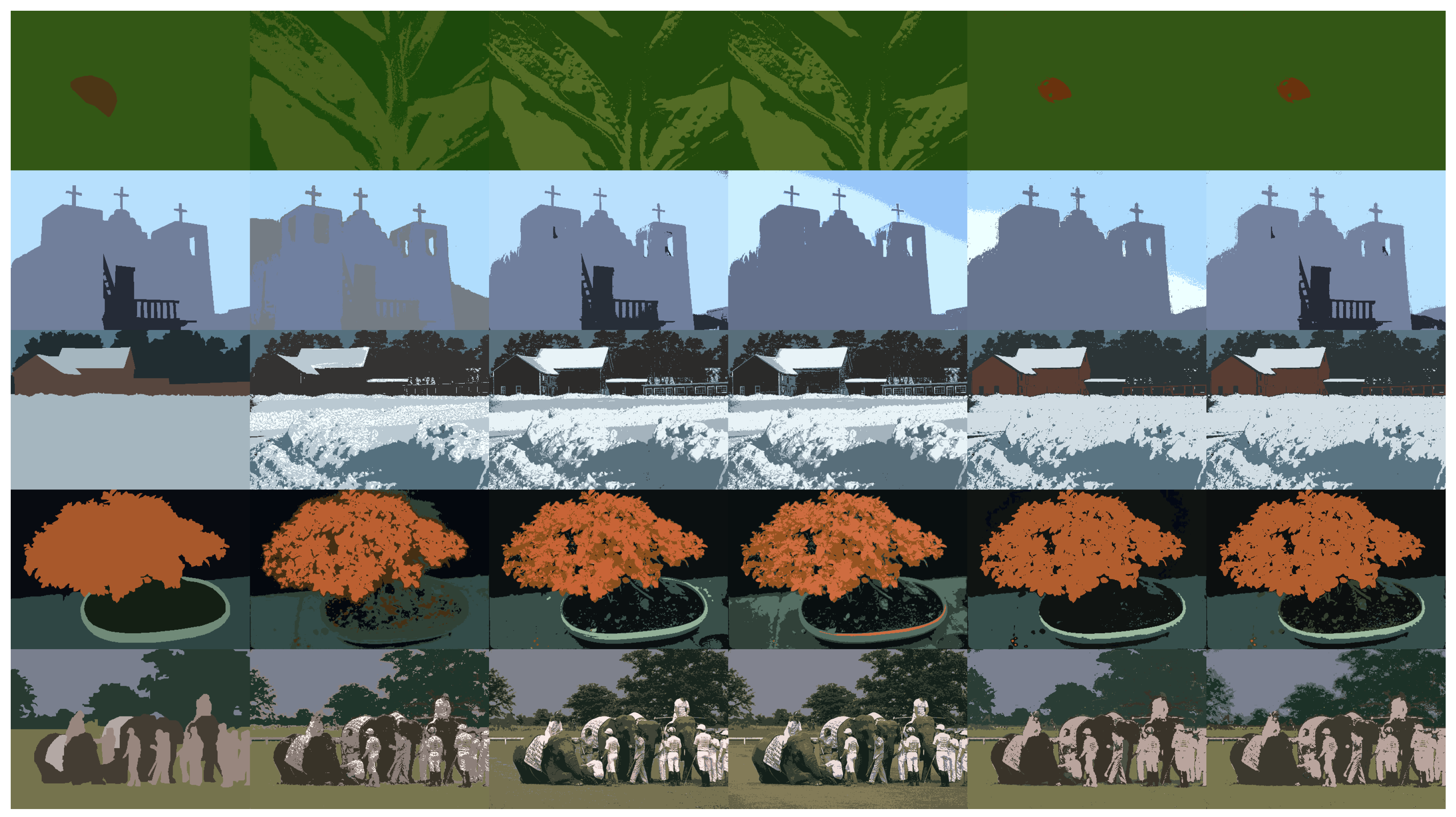
In the first image, we target two segments, a green background and a red ladybug. In the second image, 24063, we target three segments: house (white), door and balcony (brown), and sky (blue). The third image, 97033, would ideally have four segments, house (brown), snow (white), forest (green), and sky (blue). In the fourth image, 353013, there are five distinguishable colors (table, flowerpot, earth, flower, and background), so five segments, and in the fifth image there are six (earth, elephants, jockeys, blankets, forest, and sky). We summarized all qualitative results in Figure 7 and quantitative results in Table 3. For the quantitative results, we only report Precision P, Recall R, Dice score F 1 , and Jaccard score J because the true segmentation and the predicted segmentation contain the same number of segments. They seem to be sufficiently informative.
From the reported qualitative and quantitative results, it is evident that the merging of the mixture components leads to a better segmentation of the image, both by the highest obtained metric value and by the visual inspection of the segmentation. Moreover, it is clear that the merging of numerous components circumvents the problems caused by the representation of the segment by one component (or cluster for KMEANS and FCMEANS), which are mostly caused by obtaining the locally optimal cluster solution. The algorithms used here would inevitably find a more suitable local clustering solution if we further perturb the initial parameters. However, this could become impractical and computationally infeasible.

7.2.2. Optimal Segmentation Results on Berkley Image Segmetation Dataset

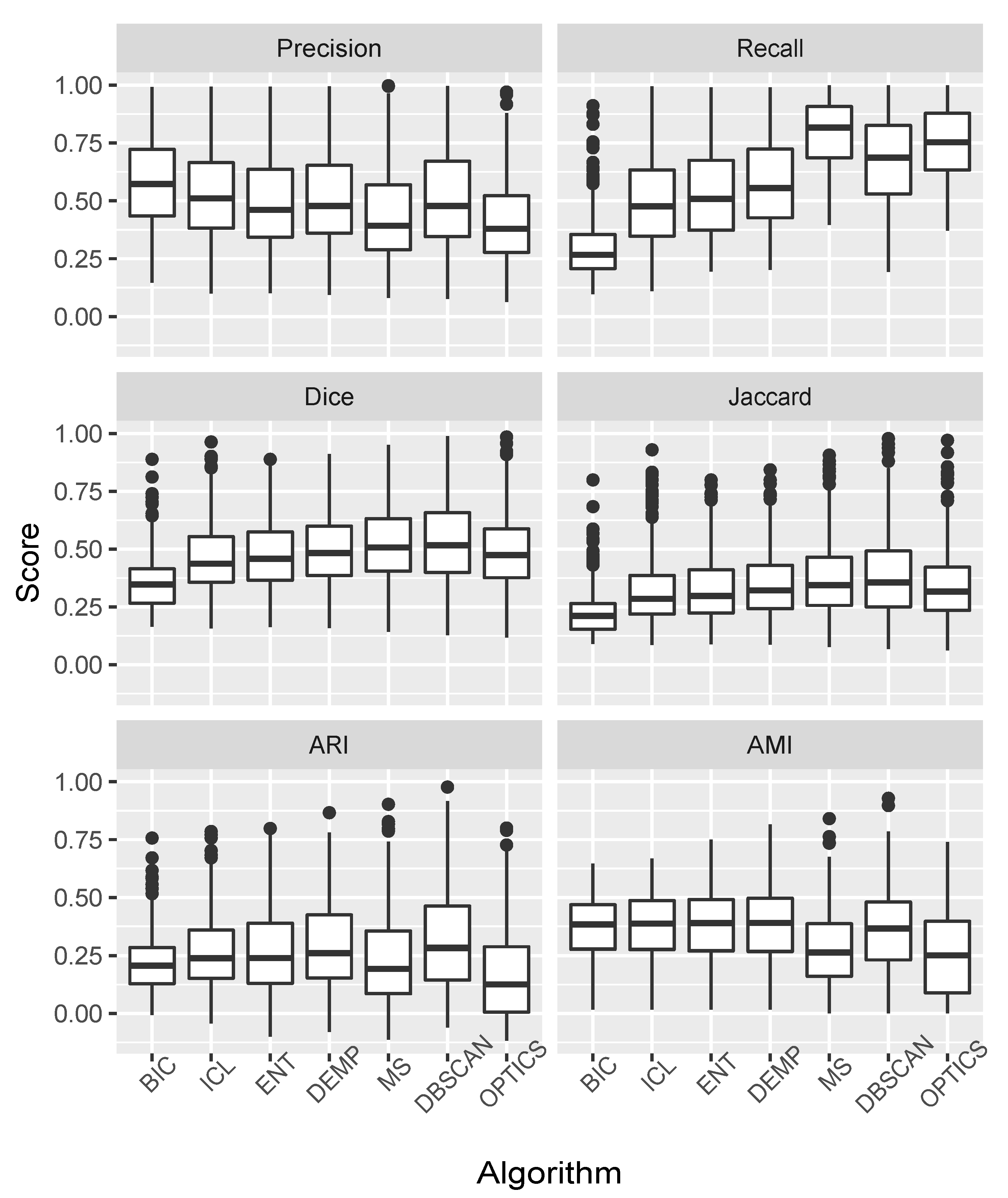
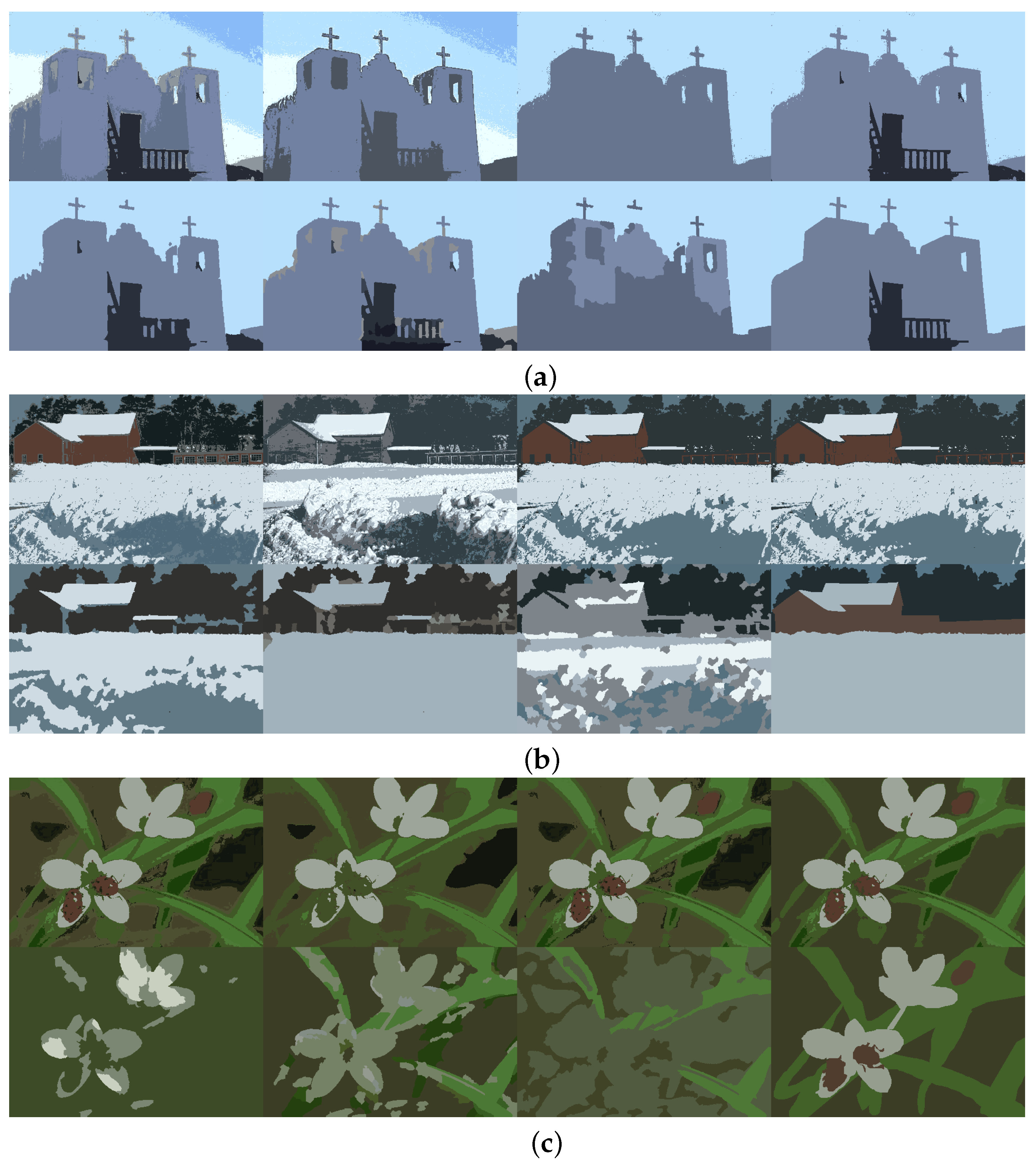
In the second part of the experiment, we are interested in empirically investigating the optimal segmentation that results from the heuristic described in Section 5. In the first part of the experiment, we manually determined the optimal number of segments based on the image under study. Thus, we limited ourselves to a smaller number of images for comparison. Here, the heuristic selects the optimal segmentation, i.e., the number of segments is determined automatically; therefore, it is plausible to analyze it on the entire dataset. The empirical study was enriched by comparisons with, in addition to the segmentation results obtained with the ICL criterion and the BIC criterion without subsequent merging, the clustering algorithms of the second group (MS, DBSCAN, and OPTICS), which can also provide optimal segmentation.The qualitative results of segmentation by using different algorithms is provided in Figure 8 and Table 4. We have also added some qualitative results in Figure 9 to further illustrate the segmentation of different algorithms. Table 4 shows the averaged metrics for each algorithm over the entire dataset. A better representation is provided by the boxplots for each algorithm and metric in Figure 8, which we can also use to examine scatter.
The results reported here are similar and mostly better than the values in [44]. This could be due to the different setting of the experimental parameters and the different implementation of the algorithm, but we find it interesting. Since the BIC and ICL algorithms returned many segments, and generally more than the other methods studied, which can be further verified in Figure 9, the precision value was high and the recall value was low, as expected. Since the clustering algorithms MS, DBSCAN, and OPTICS preferred a smaller number of segments, the recall value was high and the precision was low. This clustering was also highly dependent on the superpixels obtained. First, the superpixels greatly reduced the number of pixels (we chose about 1000 superpixels), reducing the color variations of small objects while preserving the variations of larger objects. This can also be seen in Figure 9. The ladybugs in Figure 9c or the house in Figure 9b, or rather, their respective segments are missing and were merged with others. The merging algorithms were mostly in the middle, with DEMP consistently better than ENT. The AMI value was the best of all with the DEMP algorithm. ARI’s slightly higher scores with the DBSCAN algorithm than with DEMP are due to the fact that many images contain a large portion of the scene with background that was correctly segmented in most cases. Again, both the merging algorithms and the heuristics were inadequate because the optimal segmentation favored more than one segment for the background. Finally, examination of the scatter of the metric values from Figure 8 suggests that the BIC algorithm has the least variation (i.e., the box with the lowest height). This, in turn, could be related to the fact that the BIC algorithm always had the highest number of segments. Therefore, it is expected that the values of the metrics obtained for different images would vary less. On the other hand, with fewer segments, the values may vary greatly from the expected values, resulting in very different metric values for different images.

7.3. Comparisons of Computational Times

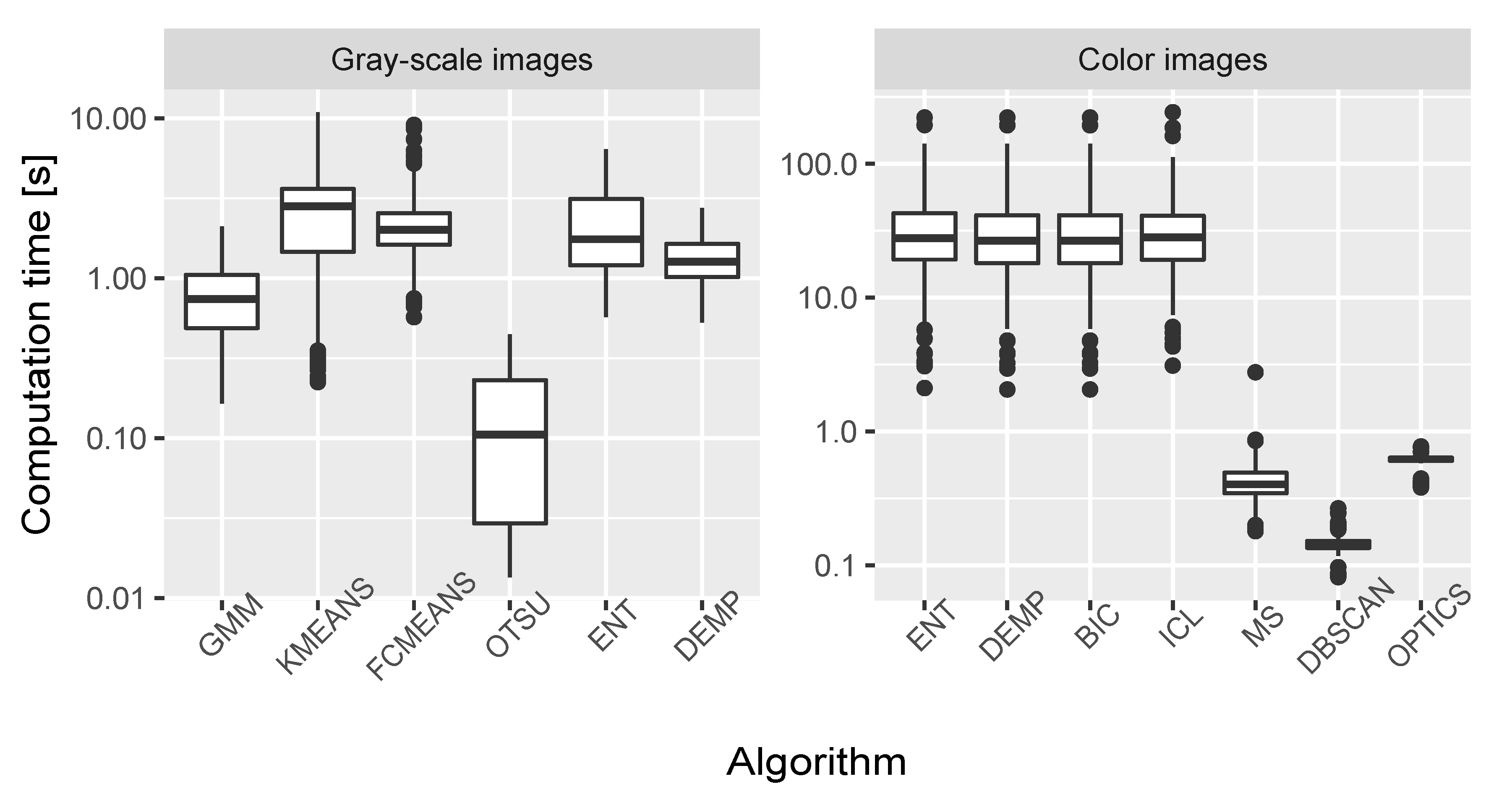
The final reports address the computation time required for each algorithm. Theoretically, the algorithms used here should be evaluated until the maximum number of iterations is exhausted, as noted in Refs. [28,39]. In this case, their time complexity is polynomial. Empirically, however, it turns out that these algorithms perform differently due to their slightly different implementations or approximations used, etc. Here, we focus on the empirical results obtained during runtime. Since the gray-scale images have only one value per pixel and the color images have three, we split the results to obtain a better understanding of the differences.
We provide the results again in the form of boxplots of the computation times for each algorithm and both datasets, one representing the gray-scale images and the other the color images, in Figure 10 and the average computation times over both datasets in Table 5. For the gray-scale images, it can be seen that the single REBMIX and EM strategy with K = 256 used for mixture estimation in the R package rebmix yields similarly fast results as the Gaussian mixture implementation of sklearn, although it estimates at least 15 more candidate mixture models, as indicated by the parameter cmax. This is also true for the KMEANS and FCMEANS algorithms used. OTSU was significantly faster, but this was to be expected due to its simple calculations. On the other hand, when comparing the color images, it looks like the mixture model approaches are abundantly exhaustive compared to their counterparts MS, DBSCAN, and OPTICS. It should be noted that the MS, DBSCAN, and OPTICS algorithms ran on largely shrunken data sets with only 1000 values obtained by SEEDS superpixel, as opposed to the mixture approach which ran on the full image resolution. The image resolution was 480 × 320, giving 153,600 pixel values, which means that the data sets for the mixture model were 150 times larger. One of the main reasons why the superpixels are used at all is that the MS, DBSCAN and OPTICS algorithms would not provide segmentation in an acceptable time to even consider them here. Therefore, the direct comparison of the computation times obtained is somewhat unfair, yet the time performance of the mixture model for color images is definitely not pleasing. Finally, ENT merging seems to be somewhat slower, at least for the gray-scale images. This is somewhat unexpected, since the number of operations is the same for DEMP and ENT merging. The only difference we think is plausible is that ENT merging requires repeated log calculation, which could cause this overhead.

8. Discussion

Merging components of a mixture model based on entropy or misclassification criteria seems to be a very useful approach to quickly improve image segmentation. Indeed, using a model selection procedure and a non-clustering information criterion such as BIC allows greater flexibility in image segmentation than simply using a clustering information criterion, e.g., ICL. The explanation for this lies in the fact that the segment-wise distribution differs from the Gaussian distribution for many images. However, the Gaussian distribution is interesting because of its simple definition and straightforward application. The segment color distribution of a given image may be multimodal or skewed, and the BIC criterion would be sufficient to model the underlying PDF of the image, but the cost is the large number of components. ICL reduces the number of components by penalizing highly overlapping components. The price, however, is that such components may not be well suited for modeling individual segments. We have seen that neither of them is capable of handling image segmentation on its own. Merging components fixes this problem and improves image segmentation and thus the application of the mixture model.
However, upon visual inspection of the segmentation, we noticed that the two merge criteria introduced seem to suffer from the obvious drawback of hierarchical merging of components. More precisely, only one pair of components is merged in each stage of the merging process. In this way, the merge estimation is simplified because in each stage the merge criterion is recalculated for the remaining untouched and merged components. However, this presents an obvious problem when the final clustering solution is not just a few stages away from the original clustering solution. Both criteria clearly focus on merging smaller components with larger ones, and likewise on merging smaller clusters with larger ones. At each stage, they increase the size of the already large cluster, so to speak. For example, if the final merge is 10 stages away from the original solution, the smaller but informative cluster has already been merged because of its size. The smaller cluster will not be merged with the larger one only if its centroid is far apart in the feature space. The optimal segmentation heuristic presented here naively fixes this, as the maximum value of Equation (20) favors more clusters of equal size. However, by using multiple merges in each stage, the problem could be circumvented. This should be considered more critically, however, as it could lead to further undesirable artifacts.
Here we have dealt with unsupervised segmentation of images using only color pixel values. It is also known that using the spatial information, i.e., pixel positions, can enrich the segmentation, especially when the image is contaminated with a lot of noise, see [12] for example. However, including this information as two additional vectors does not lead to better results, since pixel positions are not random variables. They must be explored through well-defined neighborhood systems with spatial interactions. As a starting point, we decided to explore merging only for the color pixel values, since the additional inclusion of the spatial information through a well-defined theory, such as the hidden Markov random fields [38], can only improve the results.
Finally, we would like to discuss the high computational cost of estimating the mixture model. Using the predefined value K = 256 for the pre-processing step does not reduce the size of the dataset, but only makes it more compact. We obtained sufficiently fast results for gray-scale images, but the speed was not satisfactory for color images. The value K = 256 for three-dimensional space results in 16,777,216 bins. Most of these are empty and we always obtain a smaller number of non-empty bins than the number of pixels in the image. However, most bins contain only one pixel. Decreasing the value of K also decreases the size of the dataset and affects the mixture estimation, especially with the algorithm EM. On the other hand, if we reduce the value of K to K = 50 , we obtain significantly better computation times than all other algorithms. Nevertheless, the reduction should be critically evaluated and some guidelines need to be given, which we will further focus on in the future.
9. Conclusions

The mixture model is a compelling framework for unsupervised image segmentation. The introduction of merging components of the mixture model further improves segmentation results. Moreover, the introduction of the optimal segmentation heuristic preserves the most relevant segments. We have conducted a series of experiments on gray-scale and color images, which confirm the above statements. Table 2, Table 3 and Table 4 and the Figure 5 and Figure 8 show that the reported metrics do indeed indicate better image segmentation, which can be further evidenced by looking at the qualitative segmentation in Figure 4, Figure 7 and Figure 9. Further improvements should also be carefully considered in the future. First, the inadequacy of the hierarchical merging process discussed in the previous section could be improved. Second, pixel positions should also be included in the segmentation process in an appropriate framework. Thus, the similarity of two mixture components can be further increased or decreased by introducing spatial relationships, enriching the merging process.

Author Contributions

Conceptualization, B.P., M.N., J.K., S.O.; methodology, B.P., M.N., J.K., S.O.; investigation, B.P., M.N., J.K., S.O.; software, B.P., M.N., J.K., S.O.; writing—original draft preparation, B.P., M.N., J.K., S.O.; writing—review and editing, B.P., M.N., J.K., S.O. All authors have read and agreed to the published version of the manuscript.

Funding

The authors acknowledge financial support from the Slovenian Research Agency (research core funding No. P2-0182 entitled Development Evaluation).

Conflicts of Interest

The authors declare no conflict of interest.

References

  1. Bellocchio, E.; Crocetti, F.; Costante, G.; Fravolini, M.L.; Valigi, P. A novel vision-based weakly supervised framework for autonomous yield estimation in agricultural applications. Eng. Appl. Artif. Intell. 2022, 109, 104615. [Google Scholar] [CrossRef]
  2. Alipour, M.; Harris, D.K. Increasing the robustness of material-specific deep learning models for crack detection across different materials. Eng. Struct. 2020, 206, 110157. [Google Scholar] [CrossRef]
  3. Antonello, M.; Chiesurin, S.; Ghidoni, S. Enhancing semantic segmentation with detection priors and iterated graph cuts for robotics. Eng. Appl. Artif. Intell. 2020, 90, 103467. [Google Scholar] [CrossRef]
  4. Fernández-Sanjurjo, M.; Bosquet, B.; Mucientes, M.; Brea, V.M. Real-time visual detection and tracking system for traffic monitoring. Eng. Appl. Artif. Intell. 2019, 85, 410–420. [Google Scholar] [CrossRef]
  5. He, W.; Jiang, Z.; Ming, W.; Zhang, G.; Yuan, J.; Yin, L. A critical review for machining positioning based on computer vision. Measurement 2021, 184, 109973. [Google Scholar] [CrossRef]
  6. Gupta, A.; Anpalagan, A.; Guan, L.; Khwaja, A.S. Deep learning for object detection and scene perception in self-driving cars: Survey, challenges, and open issues. Array 2021, 10, 100057. [Google Scholar] [CrossRef]
  7. Victória Matias, A.; Atkinson Amorim, J.G.; Buschetto Macarini, L.A.; Cerentini, A.; Casimiro Onofre, A.S.; De Miranda Onofre, F.B.; Daltoé, F.P.; Stemmer, M.R.; von Wangenheim, A. What is the state of the art of computer vision-assisted cytology? A Systematic Literature Review. Comput. Med Imaging Graph. 2021, 91, 101934. [Google Scholar] [CrossRef]
  8. Sefidpour, A.; Bouguila, N. Spatial color image segmentation based on finite non-Gaussian mixture models. Expert Syst. Appl. 2012, 39, 8993–9001. [Google Scholar] [CrossRef]
  9. Shi, X.; Li, Y.; Zhao, Q. Flexible Hierarchical Gaussian Mixture Model for High-Resolution Remote Sensing Image Segmentation. Remote Sens. 2020, 12, 1219. [Google Scholar] [CrossRef] [Green Version]
  10. Wei, D.; Wang, Z.; Si, L.; Tan, C.; Lu, X. An image segmentation method based on a modified local-information weighted intuitionistic Fuzzy C-means clustering and Gold-panning Algorithm. Eng. Appl. Artif. Intell. 2021, 101, 104209. [Google Scholar] [CrossRef]
  11. Chen, Y.; Cheng, N.; Cai, M.; Cao, C.; Yang, J.; Zhang, Z. A spatially constrained asymmetric Gaussian mixture model for image segmentation. Inf. Sci. 2021, 575, 41–65. [Google Scholar] [CrossRef]
  12. Wei, T.; Wang, X.; Li, X.; Zhu, S. Fuzzy subspace clustering noisy image segmentation algorithm with adaptive local variance & non-local information and mean membership linking. Eng. Appl. Artif. Intell. 2022, 110, 104672. [Google Scholar]
  13. Ji, Z.; Huang, Y.; Xia, Y.; Zheng, Y. A robust modified Gaussian mixture model with rough set for image segmentation. Neurocomputing 2017, 266, 550–565. [Google Scholar] [CrossRef]
  14. Long, J.; Shelhamer, E.; Darrell, T. Fully convolutional networks for semantic segmentation. In Proceedings of the IEEE Conference on Computer Vision and Pattern Recognition, Boston, MA, USA, 7–12 June 2015; pp. 3431–3440. [Google Scholar]
  15. Yang, H.Y.; Wang, X.Y.; Zhang, X.Y.; Bu, J. Color texture segmentation based on image pixel classification. Eng. Appl. Artif. Intell. 2012, 25, 1656–1669. [Google Scholar] [CrossRef]
  16. Li, S.; Fevens, T.; Krzyżak, A.; Li, S. Automatic clinical image segmentation using pathological modeling, PCA and SVM. Eng. Appl. Artif. Intell. 2006, 19, 403–410. [Google Scholar] [CrossRef]
  17. Chen, J.; Zheng, H.; Lin, X.; Wu, Y.; Su, M. A novel image segmentation method based on fast density clustering algorithm. Eng. Appl. Artif. Intell. 2018, 73, 92–110. [Google Scholar] [CrossRef]
  18. Kumar, V.; Chhabra, J.K.; Kumar, D. Automatic cluster evolution using gravitational search algorithm and its application on image segmentation. Eng. Appl. Artif. Intell. 2014, 29, 93–103. [Google Scholar] [CrossRef]
  19. Katunin, A.; Nagode, M.; Oman, S.; Cholewa, A.; Dragan, K. Monitoring of Hidden Corrosion Growth in Aircraft Structures Based on D-Sight Inspections and Image Processing. Sensors 2022, 22, 7616. [Google Scholar] [CrossRef]
  20. Wronkowicz-Katunin, A.; Katunin, A.; Nagode, M.; Klemenc, J. Classification of Cracks in Composite Structures Subjected to Low-Velocity Impact Using Distribution-Based Segmentation and Wavelet Analysis of X-ray Tomograms. Sensors 2021, 21, 8342. [Google Scholar] [CrossRef]
  21. Panić, B.; Klemenc, J.; Nagode, M. Gaussian Mixture Model Based Classification Revisited: Application to the Bearing Fault Classification. Stroj. Vestnik/J. Mech. Eng. 2020, 66, 215–226. [Google Scholar] [CrossRef] [Green Version]
  22. Santos, A.M.; de Carvalho Filho, A.O.; Silva, A.C.; de Paiva, A.C.; Nunes, R.A.; Gattass, M. Automatic detection of small lung nodules in 3D CT data using Gaussian mixture models, Tsallis entropy and SVM. Eng. Appl. Artif. Intell. 2014, 36, 27–39. [Google Scholar] [CrossRef]
  23. Celeux, G.; Govaert, G. Gaussian parsimonious clustering models. Pattern Recognit. 1995, 28, 781–793. [Google Scholar] [CrossRef] [Green Version]
  24. Ye, X.; Xi, P.; Nagode, M. Extension of REBMIX algorithm to von Mises parametric family for modeling joint distribution of wind speed and direction. Eng. Struct. 2019, 183, 1134–1145. [Google Scholar] [CrossRef]
  25. Vacher, J.; Launay, C.; Coen-Cagli, R. Flexibly regularized mixture models and application to image segmentation. Neural Netw. 2022, 149, 107–123. [Google Scholar] [CrossRef] [PubMed]
  26. Cheng, N.; Cao, C.; Yang, J.; Zhang, Z.; Chen, Y. A spatially constrained skew Student’st mixture model for brain MR image segmentation and bias field correction. Pattern Recognit. 2022, 128, 108658. [Google Scholar] [CrossRef]
  27. Nguyen, T.M.; Wu, Q.J. Dirichlet Gaussian mixture model: Application to image segmentation. Image Vis. Comput. 2011, 29, 818–828. [Google Scholar] [CrossRef]
  28. Panić, B.; Klemenc, J.; Nagode, M. Improved initialization of the EM algorithm for mixture model parameter estimation. Mathematics 2020, 8, 373. [Google Scholar] [CrossRef] [Green Version]
  29. Son, L.H.; Tuan, T.M. Dental segmentation from X-ray images using semi-supervised fuzzy clustering with spatial constraints. Eng. Appl. Artif. Intell. 2017, 59, 186–195. [Google Scholar] [CrossRef]
  30. Stosic, D.; Stosic, D.; Ludermir, T.B.; Ren, T.I. Natural image segmentation with non-extensive mixture models. J. Vis. Commun. Image Represent. 2019, 63, 102598. [Google Scholar] [CrossRef]
  31. Sun, H.; Yang, X.; Gao, H. A spatially constrained shifted asymmetric Laplace mixture model for the grayscale image segmentation. Neurocomputing 2019, 331, 50–57. [Google Scholar] [CrossRef]
  32. Do, T.M.T.; Artières, T. Learning mixture models with support vector machines for sequence classification and segmentation. Pattern Recognit. 2009, 42, 3224–3230. [Google Scholar] [CrossRef]
  33. Zeng, S.; Huang, R.; Kang, Z.; Sang, N. Image segmentation using spectral clustering of Gaussian mixture models. Neurocomputing 2014, 144, 346–356. [Google Scholar] [CrossRef]
  34. Baudry, J.P.; Raftery, A.E.; Celeux, G.; Lo, K.; Gottardo, R. Combining Mixture Components for Clustering. J. Comput. Graph. Stat. 2010, 19, 332–353. [Google Scholar] [CrossRef] [PubMed] [Green Version]
  35. Hennig, C. Methods for merging Gaussian mixture components. Adv. Data Anal. Classif. 2010, 4, 3–34. [Google Scholar] [CrossRef]
  36. Nagode, M.; Fajdiga, M. The REBMIX Algorithm for the Univariate Finite Mixture Estimation. Commun. Stat. Theory Methods 2011, 40, 876–892. [Google Scholar] [CrossRef]
  37. Nagode, M.; Fajdiga, M. The REBMIX Algorithm for the Multivariate Finite Mixture Estimation. Commun. Stat. Theory Methods 2011, 40, 2022–2034. [Google Scholar] [CrossRef]
  38. McLachlan, G.; Peel, D. Finite Mixture Models, 1st ed.; John Wiley & Sons: Hoboken, NJ, USA, 2000. [Google Scholar]
  39. Panić, B.; Klemenc, J.; Nagode, M. Optimizing the Estimation of a Histogram-Bin Width—Application to the Multivariate Mixture-Model Estimation. Mathematics 2020, 8, 1090. [Google Scholar] [CrossRef]
  40. Schwarz, G. Estimating the Dimension of a Model. Ann. Stat. 1978, 6, 461–464. [Google Scholar] [CrossRef]
  41. Zhao, J.; Jin, L.; Shi, L. Mixture model selection via hierarchical BIC. Comput. Stat. Data Anal. 2015, 88, 139–153. [Google Scholar] [CrossRef]
  42. Biernacki, C.; Celeux, G.; Govaert, G. Assessing a mixture model for clustering with the integrated completed likelihood. IEEE Trans. Pattern Anal. Mach. Intell. 2000, 22, 719–725. [Google Scholar] [CrossRef]
  43. Martin, D.; Fowlkes, C.; Tal, D.; Malik, J. A Database of Human Segmented Natural Images and its Application to Evaluating Segmentation Algorithms and Measuring Ecological Statistics. In Proceedings of the 8th Int’l Conference Computer Vision, Vancouver, BC, Canada, 7–14 July 2001; Voume 2; pp. 416–423. [Google Scholar]
  44. Aksac, A.; Özyer, T.; Alhajj, R. CutESC: Cutting edge spatial clustering technique based on proximity graphs. Pattern Recognit. 2019, 96, 106948. [Google Scholar] [CrossRef]
  45. Azzalini, A.; Bowman, A.W. A Look at Some Data on the Old Faithful Geyser. J. R. Stat. Society. Ser. C Appl. Stat. 1990, 39, 357–365. [Google Scholar] [CrossRef]
  46. Akaike, H. A new look at the statistical model identification. IEEE Trans. Autom. Control 1974, 19, 716–723. [Google Scholar] [CrossRef]
  47. Scrucca, L. A fast and efficient Modal EM algorithm for Gaussian mixtures. Stat. Anal. Data Min. ASA Data Sci. J. 2021, 14, 305–314. [Google Scholar] [CrossRef]
  48. Nagode, M.; Klemenc, J. Modelling of Load Spectra Containing Clusters of Less Probable Load Cycles. Int. J. Fatigue 2021, 143, 106006. [Google Scholar] [CrossRef]
  49. Nagode, M. Finite Mixture Modeling via REBMIX. J. Algorithms Optim. 2015, 3, 14–28. [Google Scholar] [CrossRef]
  50. Swain, M.; Tripathy, T.T.; Panda, R.; Agrawal, S.; Abraham, A. Differential exponential entropy-based multilevel threshold selection methodology for colour satellite images using equilibrium-cuckoo search optimizer. Eng. Appl. Artif. Intell. 2022, 109, 104599. [Google Scholar] [CrossRef]
  51. Mamta; Hanmandlu, M. A new entropy function and a classifier for thermal face recognition. Eng. Appl. Artif. Intell. 2014, 36, 269–286. [Google Scholar] [CrossRef]
  52. Kurban, R.; Durmus, A.; Karakose, E. A comparison of novel metaheuristic algorithms on color aerial image multilevel thresholding. Eng. Appl. Artif. Intell. 2021, 105, 104410. [Google Scholar] [CrossRef]
  53. Robin, S.; Scrucca, L. Mixture-based estimation of entropy. Comput. Stat. Data Anal. 2023, 177, 107582. [Google Scholar] [CrossRef]
  54. Kittaneh, O.A.; Khan, M.A.U.; Akbar, M.; Bayoud, H.A. Average Entropy: A New Uncertainty Measure with Application to Image Segmentation. Am. Stat. 2016, 70, 18–24. [Google Scholar] [CrossRef]
  55. Vinh, N.X.; Epps, J.; Bailey, J. Information theoretic measures for clusterings comparison: Variants, properties, normalization and correction for chance. J. Mach. Learn. Res. 2010, 11, 2837–2854. [Google Scholar]
  56. Franti, P.; Sieranoja, S. How much can k-means be improved by using better initialization and repeats? Pattern Recognit. 2019, 93, 95–112. [Google Scholar] [CrossRef]
  57. Peizhuang, W. Pattern Recognition with Fuzzy Objective Function Algorithms (James C. Bezdek). SIAM Rev. 1983, 25, 442. [Google Scholar] [CrossRef]
  58. Comaniciu, D.; Meer, P. Mean shift: A robust approach toward feature space analysis. IEEE Trans. Pattern Anal. Mach. Intell. 2002, 24, 603–619. [Google Scholar] [CrossRef] [Green Version]
  59. Schubert, E.; Sander, J.; Ester, M.; Kriegel, H.P.; Xu, X. DBSCAN Revisited, Revisited: Why and How You Should (Still) Use DBSCAN. Acm Trans. Database Syst. (TODS) 2017, 42, 1–21. [Google Scholar] [CrossRef]
  60. Schubert, E.; Gertz, M. Improving the Cluster Structure Extracted from OPTICS Plots. In Proceedings of the Conference “Lernen, Wissen, Daten, Analysen”, LWDA 2018. Mannheim, Germany, 22–24 August 2018; Gemulla, R., Ponzetto, S.P., Bizer, C., Keuper, M., Stuckenschmidt, H., Eds.; 2018; Volume 2191, pp. 318–329. [Google Scholar]
  61. Pedregosa, F.; Varoquaux, G.; Gramfort, A.; Michel, V.; Thirion, B.; Grisel, O.; Blondel, M.; Prettenhofer, P.; Weiss, R.; Dubourg, V.; et al. Scikit-learn: Machine Learning in Python. J. Mach. Learn. Res. 2011, 12, 2825–2830. [Google Scholar]
  62. Bergh, M.V.D.; Boix, X.; Roig, G.; Capitani, B.D.; Gool, L.V. Seeds: Superpixels extracted via energy-driven sampling. In European Conference on Computer Vision; Springer: Berlin/Heidelberg, Germany, 2012; pp. 13–26. [Google Scholar]
  63. Liu, Y.; Yao, J.; Lu, X.; Xie, R.; Li, L. DeepCrack: A deep hierarchical feature learning architecture for crack segmentation. Neurocomputing 2019, 338, 139–153. [Google Scholar] [CrossRef]
  64. Munoz-Minjares, J.; Vite-Chavez, O.; Flores-Troncoso, J.; Cruz-Duarte, J.M. Alternative Thresholding Technique for Image Segmentation Based on Cuckoo Search and Generalized Gaussians. Mathematics 2021, 9, 2287. [Google Scholar] [CrossRef]
Figure 1. Model selection illustrated.
Mathematics 10 04301 g001
Figure 2. Image segmentation task.
Mathematics 10 04301 g002
Figure 3. Old faithful dataset with two and three clustering schemes from estimated two- and three component Gaussian mixture models (GMM). (a) Old faithful dataset. (b) Two-component GMM. (c) Three-component GMM.
Mathematics 10 04301 g003
Figure 4. Segmentation of crack images with different clustering algorithms. First row: gray-scale image; true segmentation; GMM; KMEANS. Second row: FCMEANS; OTSU; ENT; DEMP.
Mathematics 10 04301 g004
Figure 5. Boxplots of the metric distribution using different clustering algorithms for the crack image segmentation dataset.
Mathematics 10 04301 g005
Figure 6. Selected images from the Berkley image segmentation dataset. Image identifiers are: 35058, 24063, 97033, 353013, 361084.
Mathematics 10 04301 g006
Figure 7. Image segmentation with different clustering algorithms. First column: True segmentation; Second column: GMM; Third column: KMEANS; Fourth column: FCMEANS; Fifth column: ENT; Sixth column: DEMP.
Mathematics 10 04301 g007
Figure 8. Boxplots of the metric distribution using different clustering algorithms for the Berkley image segmentation dataset.
Mathematics 10 04301 g008
Figure 9. Segmentation results on different images from Berkley image segmentation dataset. First row: BIC, ICL, DEMP, and ENT algorithm. Second row: MS, DBSCAN, and OPTICS algorithm. Last image in second row is true segmentation. (a) Segmentation results of different algorithms on image 24063. (b) Segmentation results of different algorithms on image 97033. (c) Segmentation results of different algorithms on image 35008.
Mathematics 10 04301 g009
Figure 10. Boxplots of the distribution of computational time using different clustering algorithms for the two datasets used (the dataset for crack segmentation is referred to as gray-scale images and the dataset for Berkley image segmentation is referred to as color images).
Mathematics 10 04301 g010
Table 1. Values of BIC for estimated Gaussian mixture model with different numbers of components.
Gaussian Mixture ModelTwo Component SolutionThree Component Solution
AIC22842274
BIC23202314
ICL23202357
Table 2. Averaged metric values obtained on crack segmentation dataset. The best values are in bold.
Metric↓/Algorithm→GMMKMEANSFCMEANSOTSUENTDEMP
Precision (P)45.639.028.238.978.470.9
Recall (R)88.592.694.492.663.473.7
Dice ( F 1 )54.445.334.845.261.965.3
Jaccard (J)42.636.126.636.049.754.1
Table 3. Quantitative results of segmentation quality of selected images with different clustering algorithms. The best values are in bold.
Precision score (P)
AlgorithmGMMKMEANSFCMEANSENTDEMP
Image
35058 9494.294.296.896.8
24063 91.195.780.381.796.4
97033 73.468.767.983.783.7
353013 77.058.458.465.769
361084 76.653.151.180.975.7
Recall score (R)
AlgorithmGMMKMEANSFCMEANSENTDEMP
Image
35058 50.454.454.399.999.9
24063 91.195.780.381.796.4
97033 73.468.767.983.783.7
353013 64.863.756.884.785.1
361084 73.057.045.876.569.4
Dice score (F1)
AlgorithmGMMKMEANSFCMEANSENTDEMP
Image
35058 65.669.068.998.398.3
24063 81.893.978.984.895.7
97033 55.749.448.867.067.0
353013 70.460.957.674.076.2
361084 74.755.048.378.672.4
Jaccard score (J)
AlgorithmGMMKMEANSFCMEANSENTDEMP
Image
35058 48.852.652.596.796.7
24063 69.388.565.273.691.8
97033 38.632.832.350.350.3
353013 54.343.840.458.761.6
361084 59.737.931.964.856.7
Table 4. Averaged metrics obtained with the Berkley image segmentation dataset. The best values are in bold.
Metric↓/Algorithm→BICICLENTDEMPMSDBSCANOPTICS
Precision (P)58.353.650.251.444.451.141.6
Recall (R)30.250.153.857.478.966.875.7
Dice (F1)36.146.747.549.852.753.749.5
Jaccard (J)22.932.232.834.938.439.535.1
ARI2226.826.829.324.731.417.3
AMI36.937.237.938.428.136.225.2
Table 5. Average value of computation time over for each algorithm.
Gray-scale images
AlgorithmGMMKMEANSFCMEANSOTSUENTDEMP
Computation time (s)0.7862.6712.2720.1392.2671.375
Color images
AlgorithmBICICLENTDEMPMSDBSCANOPTICS
Computation time (s)32.8233.7533.8632.830.4290.1450.591
Publisher’s Note: MDPI stays neutral with regard to jurisdictional claims in published maps and institutional affiliations.