


Abstract
This study examines whether daily machine learning stock rankings based on technical information contain out-of-sample ordering information and whether that information can be converted into economically implementable returns. Using a dynamically screened Nasdaq source universe from 2021 to 2026, four XGBoost objectives are evaluated in a chronological walk-forward design. Test NDCG converges to 0.495–0.504, but permutation analysis places the corresponding random-ranking mean near 0.45, indicating statistically detectable but modest cross-sectional ordering information. Economic performance is substantially weaker. Under the execution convention implied by the next-day open-to-close target, every invested portfolio is bought at the open and liquidated at the close, so round-trip turnover equals two. Pseudo-Huber Top-1, treated as an ex-post concentration diagnostic, produces a 34.9% gross annual geometric return with 89.5% volatility and an 86.5% maximum drawdown; the Newey–West mean-return test is not significant (p = 0.106). At five basis points per trading leg, its zero-cash net CAGR falls to 4.8%; crediting idle capital with the daily risk-free rate raises total-return CAGR to 9.3%, but the excess-return inference is unchanged (p = 0.297). A matched-horizon regression on SPY open-to-close returns yields a statistically insignificant net annualized alpha (p = 0.436). Hansen’s SPA test across the synchronized 12-strategy family gives p = 0.207, and the Deflated Sharpe Ratio probability for Pseudo-Huber Top-1 is 0.462. The result is also highly time- and tail-dependent. The evidence therefore supports a distinction between statistically detectable ranking information and robust implementable abnormal performance rather than a persistent trading anomaly.
Keywords:
AI; machine learning; stock ranking; technical indicators; transaction costs; out-of-sample evaluation; portfolio implementation JEL Classification:
C45; G11; G17
1. Introduction
Machine learning has become an important tool for studying the cross-section of expected stock returns. Flexible nonlinear methods can capture interactions and threshold effects that are difficult to represent with conventional linear specifications (Gu et al., 2020; Freyberger et al., 2020; Leippold et al., 2022). Yet, predictive ordering and investable abnormal performance are distinct empirical objects. A ranking can contain statistically detectable information while still failing economically because the signal is unstable, concentrated in extreme observations, or too costly to trade. This distinction is especially important at daily horizons, where the effective time-series sample is measured in trading dates, and portfolio turnover can dominate modest expected-return differences.
This paper studies that tension in daily cross-sectional equity selection using technical information. Technical variables summarize recent price dynamics, volatility, reversal, trading activity, and market context, but technical strategies are also especially exposed to specification search and data-snooping concerns (Brock et al., 1992; Sullivan et al., 1999; Harvey et al., 2016). We therefore ask two sequential questions: do the models rank the subsequent cross-section better than a random ordering, and, if so, does that ranking information survive realistic implementation, risk adjustment, temporal instability, and multiplicity?
The empirical design compares four XGBoost objectives—Pseudo-Huber regression, downside-penalized regression, pairwise ranking, and NDCG-oriented ranking—using the same information set and chronological walk-forward protocol. The models use 196 technical predictors and are evaluated over 1094 out-of-sample test iterations. The effective independent time dimension is therefore the sequence of test dates rather than the much larger number of stock date observations. This distinction is important when interpreting high-dimensional estimation with 105 training dates and 196 raw or 392 combined inputs.
Portfolio implementation is evaluated after model scoring and configuration selection. Because the dependent variable is the next-day open-to-close return, the revised accounting adopts a consistent intraday execution convention: positions are entered at the next open and liquidated at that close. A fully invested trading day therefore has round-trip turnover equal to two, irrespective of whether the same security is selected on adjacent dates. The earlier transition-overlap turnover convention was inconsistent with the return horizon and has been removed from all revised net-performance calculations. With a constant round-trip cost across fully invested candidate configurations, trading cost does not discriminate among candidates within a date; the finance component of the adaptive rule is therefore ranked by validation return rather than by overlap-based transition turnover.
We additionally report a Top-1 concentration diagnostic derived from the retained upper-tail model rankings. This diagnostic was introduced after examination of the broader concentration results and is therefore not treated as a pre-specified validation choice. Its purpose is to assess whether unusually large realized outcomes are concentrated at the extreme upper tail of the long-only ranking, while the subsequent inference explicitly accounts for strategy multiplicity.
The largest gross point estimate occurs for Pseudo-Huber Top-1. Under the corrected intraday accounting, its annual geometric return is 34.9%, annual volatility is 89.5%, and maximum drawdown is 86.5%. The mean-return Newey–West statistic is 1.62 (p = 0.106), however, and the result is highly time-dependent: the first half of the test period has a gross geometric return of 154.9%, whereas the second half is −28.9%. Calendar year performance is positive and extremely large early in the sample but negative in 2024, 2025, and 2026 on a geometric basis. We therefore treat Top-1 as an unstable concentration episode rather than evidence of a persistent expected-return anomaly.
Implementation further weakens the concentration result. At five basis points per trading leg, Pseudo-Huber Top-1 falls from a 34.9% gross CAGR to a 4.8% zero-cash net CAGR. When idle capital is credited with the daily risk-free rate, total-return CAGR is 9.3%, but the excess-return Sharpe and Newey–West inference are unchanged because the risk-free accrual is removed when excess returns are formed. The net mean-return p-value is 0.297. A matched-horizon SPY open-to-close regression gives an annualized net alpha of 33.3% with p = 0.436, while close-to-close CAPM/FF3/FF5 estimates are retained only as secondary, horizon-mismatched robustness checks. Hansen’s SPA test across the synchronized 12-strategy family gives p = 0.207, and the Deflated Sharpe Ratio probability for Pseudo-Huber Top-1 is 0.462. These diagnostics reinforce the conclusion that the economically large gross point estimate is not robust evidence of abnormal performance.
High turnover is distinct from market participation. At a $50,000 capital level, a Pseudo-Huber Top-1 one-way trade has median participation of approximately 0.103% of contemporaneous ADV20; the 95th percentile is 0.899%, and 95.8% of one-way trade legs remain below 1% of ADV20. These figures show that the tested retail-scale notional is generally small relative to the observed dollar volume. They are not spread estimates, do not model market-on-open slippage, and do not constitute an institutional capacity analysis.
The paper contributes by separating three questions that are often conflated in short-horizon machine learning studies. First, a permutation benchmark establishes that test NDCG around 0.50 is above the random-ranking null for the paper’s relevance transformation; the models therefore contain measurable, though modest, cross-sectional ordering information. Second, economic tests show that ranking information does not translate into robust abnormal performance after round-trip costs, factor adjustment, subperiod instability, naive technical benchmarks, and multiple-testing controls. Third, the revised analysis distinguishes execution turnover from liquidity participation and reports all liquidity gates, including the $50 million and $100 million thresholds, with invested-day diagnostics.
Overall, the evidence supports a negative implementability result rather than a headline backtest. Daily technical machine learning rankings contain statistically detectable cross-sectional information, but the observed portfolio gains are unstable, tail-sensitive, and not robustly distinguishable from zero after realistic intraday accounting and multiple-testing controls. The economically relevant contribution is therefore the gap between ranking information and the tradable abnormal return.
The remainder of the paper proceeds as follows. Section 2 reviews the related literature and develops the research motivation. Section 3 describes the data, features, models, and walk-forward selection procedure. Section 4 reports predictive, portfolio, implementation, and inference results. Section 5 discusses implementation implications and extensions, and Section 6 concludes.
2. Literature Review
2.1. Machine Learning and Cross-Sectional Return Prediction
Machine learning has expanded empirical asset pricing by allowing expected returns to depend on high-dimensional and nonlinear functions of observable information. Gu et al. (2020) show that tree-based methods and neural networks improve out-of-sample return prediction relative to conventional linear approaches, with much of the gain arising from nonlinear interactions among predictors. Freyberger et al. (2020) similarly document nonlinearities in the cross-section of expected returns. Using nearly 12,000 European stocks, Fieberg et al. (2023) further show that nonlinear machine learning methods can improve both statistical and portfolio performance relative to linear benchmarks, while emphasizing that these gains vary with the market segment and liquidity. Together, this literature establishes that flexible models can improve cross-sectional return prediction, but that their economic value must be assessed through the portfolios and trading required to exploit the forecasts.
Our setting differs from the standard characteristic-based asset-pricing problem in two respects. First, the prediction horizon is one trading day rather than monthly or longer. Second, the information set consists entirely of variables observable from prices and trading activity. Technical rules have a long empirical history (Brock et al., 1992), and nonparametric technical patterns have been studied at the individual stock level (Lo et al., 2000). Neely et al. (2014) provide complementary evidence for technical indicators in aggregate equity-premium forecasting. These studies in the literature motivate the information set but do not establish that technical indicators predict the daily cross-section; that question is tested here.
These concerns motivate the chronological structure of the empirical design. Technical variables are not interpreted as standalone trading rules, and no full-sample search selects a preferred indicator. A large set of short-horizon signals enters the nonlinear models jointly, while feature representation and portfolio size are chosen only from the preceding validation window. Because the design nevertheless evaluates multiple models, hyperparameters, feature representations, and portfolio sizes, strict chronology does not by itself eliminate research-design multiplicity or backtest overfitting (Harvey et al., 2016; A. Y. Chen & Zimmermann, 2022; Anghel, 2021; Bailey et al., 2014; López de Prado, 2018; McLean & Pontiff, 2016).
2.2. Prediction Versus Ranking at the Upper Tail
Most empirical return prediction methods minimize an error defined over the entire cross-section. That objective need not coincide with the investor’s decision problem. If capital is allocated only to a few securities, accurately distinguishing the strongest opportunities may be more important than correctly ordering stocks near the middle or bottom of the predicted distribution. This difference motivates our comparison of return regression and learning-to-rank objectives.
The regression specifications estimate return magnitudes, whereas the ranking specifications target relative ordering. Pairwise ranking emphasizes whether one security is ordered above another; the NDCG-oriented specification uses a ranking surrogate intended to improve top-weighted ordering. Learning-to-rank methods have previously been applied to cross-sectional systematic strategies and stock selection (Poh et al., 2021; Song et al., 2017). The comparison is conducted within a common XGBoost framework so that differences can be interpreted primarily in terms of the learning objective rather than unrelated model classes.
This distinction is economically important because weak full-cross-sectional prediction need not imply an absence of useful information in the extreme tail. Gu et al. (2020) emphasize that the economic assessment of forecasts ultimately depends on the portfolios formed from them, rather than predictive fit alone. More broadly, flexible models can uncover nonlinear return relationships that are not well summarized by average linear associations (Freyberger et al., 2020). We extend this reasoning to a much shorter horizon by separating broad ranking accuracy from performance among the model’s highest-ranked observations.
The Top-1 portfolio is therefore treated as an ex-post concentration diagnostic rather than as a pre-specified validation choice. It was introduced to examine whether the economic results are concentrated in the highest-ranked security. The Top-1 diagnostic is not part of the adaptive K-selection grid and is not interpreted as confirmatory evidence.
2.3. Turnover, Transaction Costs, and Investor Scale
A central lesson from the portfolio implementation literature is that gross predictability can be economically misleading when it requires substantial trading. Korajczyk and Sadka (2004) show that market frictions and price impact materially affect momentum profitability and capacity, while Novy-Marx and Velikov (2016), DeMiguel et al. (2020), and Patton and Weller (2020) show more broadly that transaction costs can materially alter the apparent profitability and construction of return predictive strategies.
Transaction costs can also change the portfolio itself rather than simply reduce its realized return. DeMiguel et al. (2020) show that incorporating transaction costs alters the set of characteristics that matter for optimal portfolio construction because combining signals can reduce required trading. More recently, Jensen et al. (2026) argue that machine learning strategies should be evaluated on an implementable efficient frontier defined in terms of return net of trading costs for each level of risk. Li et al. (2026) provide a complementary approach in which portfolio generation and transaction-cost management are separated, and trades are executed only when expected gains justify their costs. This distinction is closely related to the present design, which preserves a separate prediction layer and incorporates trading costs when deciding whether a candidate portfolio configuration is economically attractive.
Our framework incorporates this issue at the configuration selection stage rather than inside the XGBoost loss. Candidate portfolios are first generated from model scores. For each candidate configuration c on decision date t, validation performance is evaluated net of the turnover required to move from the currently implemented portfolio to the candidate portfolio:
Here, denotes the candidate validation portfolio return, is the turnover required to move from the currently implemented portfolio to candidate c, and λ is the proportional cost per unit of turnover. Under the turnover convention defined formally in Section 3.6, λ = 0.0005 corresponds to five basis points per one-way dollar traded; complete replacement of a fully invested portfolio has τ = 2 and therefore costs 10 basis points. Section 4.6 evaluates a wider cost frontier.
Turnover and market participation capture different implementation frictions. Turnover measures the amount of portfolio capital reallocated, whereas trade participation compares a required trade with contemporaneous market volume. A concentrated portfolio can therefore experience near-complete daily replacement while still representing a small fraction of normal trading volume at modest capital levels (Korajczyk & Sadka, 2004; Novy-Marx & Velikov, 2016).
We consequently report both transaction-cost sensitivity and retail-scale trade participation. Required buy and sell trades are compared with contemporaneous 20-day median dollar volume. This exercise does not estimate a complete capacity curve; it separates whether the tested $50,000 portfolio requires large market participation from whether repeated execution costs can absorb its predicted return.
2.4. Research Motivation
Our analysis brings together three strands of the literature that are usually evaluated separately: nonlinear cross-sectional return prediction, rank-based security selection, and portfolio implementability. Relative to the machine learning asset pricing literature, the focus is not on maximizing broad predictive fit but on identifying where within the predicted cross-section economically useful information is concentrated. Relative to the technical trading literature, technical variables enter an out-of-sample nonlinear ranking framework rather than being evaluated individually as trading rules. Relative to the transaction cost literature, turnover enters the configuration decision before the next test portfolio is implemented, while a separate retail-scale trade participation analysis distinguishes frequent rebalancing from market volume constraints.
The resulting empirical question is deliberately narrow: can localized short-horizon predictability among the highest-ranked securities survive the trading required to exploit it, and does that answer depend on portfolio concentration and investor scale? This question provides the organizing structure for the empirical analysis that follows.
3. Data, Feature Engineering and Research Methodology
3.1. Data Collection and Investment Universe
The analysis uses daily open, high, low, close, adjusted close, and trading volume data downloaded through the yfinance interface with automatic price adjustment enabled. In Table 1 presents the timelines starting with the raw market data period runs from 2 August 2021 to 31 July 2026. After feature construction and rolling-window requirements, the out-of-sample test period runs from 21 March 2022 to 30 July 2026. The original walk-forward export contains 1094 test iterations; after alignment to realized next-trading-day benchmark and factor dates, 1093 observations are available for the revised portfolio comparisons. Security metadata correspond to Nasdaq exchange codes NMS, NGM, and NCM.
Table 1.
Study timeline and walk-forward windows.
The source-level candidate file retained for the study contains 5138 symbols assembled from Nasdaq listings and provider metadata at the 2026 collection date; a separate retained metadata file contains 454 tickers for which the required security metadata and market data workflow were available. Daily history, price, feature availability, and liquidity screens then determine the investable cross-section on each date. This source construction is not a historical point-in-time constituent database: securities that disappeared before the collection date may be absent, and the dynamic screens cannot repair that omission. No delisting-return reconstruction is claimed. All return estimates are therefore conditional on the collected source universe, and survivorship/delisting selection can affect the magnitude of the reported returns (Shumway, 1997).
For each trading day t, the eligible universe contains the securities from the source candidate set that satisfy the contemporaneous history, price, and liquidity screens. The dynamic screen allows securities to enter or leave the investable cross-section as these conditions change. All feature construction and daily eligibility decisions use information available no later than t.
where is the number of securities satisfying the point-in-time eligibility rules on date t.
The prediction panel is defined by observations () for i in , where:
Here, is the p-dimensional technical predictor vector observed by the close of date t. The dependent variable is the next-day open-to-close return, so all predictors are known before the return used for evaluation is realized.
The resulting panel is unbalanced because daily eligibility changes through time. The point-in-time screens determine whether a security from the collected source list is eligible on a given date, but they do not solve source-universe survivorship bias. In the next section presents and describes the screened panel conditional on that source list which is rather than the full historical Nasdaq stock listing population.
3.2. Sample Screening and Liquidity Filtering
A security enters the investable cross-section on day t only if it satisfies three point-in-time conditions. First, at least 35 daily observations must be available, allowing construction of predictors with lookbacks of up to 30 trading days. Second, the closing price must be at least $5. Third, the trailing 20-day median dollar volume must exceed the contemporaneous 10th percentile of the eligible cross-sectional distribution. Table 2 summarizes these screens.
Table 2.
Sample screening criteria.
Dollar volume and the screening liquidity variable are defined as:
The trailing liquidity measure is:
is the median of the most recent 20 daily dollar-volume observations available by date t. The eligibility cutoff is the contemporaneous 10th percentile of ADV20 across the available cross-section. The threshold therefore changes with market conditions and removes only the least liquid tail. ADV20 is used as a transparent liquidity and participation proxy rather than as a structural estimate of price impact (Amihud, 2002; Korajczyk & Sadka, 2004).
Table 3 summarizes the dynamic universe from the first date on which the feature and screen calculations are available. Its N = 1220 therefore refers to all dates used to characterize the eligible-universe process, whereas the walk-forward out-of-sample analysis contains 1094 test iterations (1093 after realized-date alignment in the revised benchmark and factor comparisons). These counts refer to different windows and are not competing sample sizes.
Table 3.
Dynamic investment universe after eligibility begins.
The time variation in universe size and the liquidity threshold is reported in Appendix A Figure A1 and Figure A2, respectively. Those figures are useful as diagnostics but do not need to remain in the main text.
3.3. Feature Engineering
Raw daily market data are transformed into 196 technical predictors spanning intraday structure, return continuation and reversal, trend and price displacement, volatility and downside risk, oscillators, volume and liquidity, and market context. Supplementary Table S1 reports the complete predictor catalogue and identifies the 14 market aggregate predictors that are constant across securities within a given date. Supplementary Table S2 reports the hyperparameter search specification, random seeds, retuning schedule, and regression-target scaling. Exact historical package-version strings were not preserved and are therefore not reconstructed retrospectively.
For stock i on date t, define the raw technical predictor vector as:
The model maps into either a predicted next-day return or a ranking score, depending on the learning objective, and the resulting scores are used only for the subsequent day t + 1.
The predictors are grouped into economically interpretable families to summarize model attribution and stability. These groupings do not impose restrictions on estimation; all predictors enter the corresponding XGBoost specification jointly.
In Table 4 shows the structure of all 196 predictors which are available by the close of day t, while the target is the open-to-close return on day t + 1. This horizon intentionally excludes the close-to-open gap. The revised implementation is therefore strictly intraday: positions are established at the next open and closed at the same day’s close. The study does not estimate a close-to-close alternative because that change would define a different prediction target and require model re-estimation; this limitation is stated explicitly rather than approximated with incompatible returns.
Table 4.
Technical predictor families.
Most predictors use lookback windows of 1, 2, 3, 5, 10, and 20 trading days, with selected 30-day measures providing broader context. These windows are a design choice intended to emphasize recent market information; their usefulness is evaluated out of sample rather than assumed from the one-day target horizon.
The technical indicators are not interpreted as independent trading rules. They enter nonlinear models jointly so that the fitted trees can use interactions among momentum, reversal, volatility, volume, liquidity, and market conditions. This treatment is motivated by technical pattern evidence in individual stocks and aggregate-market forecasting, while the incremental value of the full predictor set is determined by the present out-of-sample experiment (Lo et al., 2000; Neely et al., 2014). High-dimensional predictor redundancy is a further reason to rely on regularized out-of-sample estimation rather than isolated in-sample indicator tests (Kozak et al., 2020).
The analysis evaluates three representations of the predictor set. The raw representation retains the original 196 numerical features. The ranked representation maps each feature to its cross-sectional percentile position within the eligible universe on the same date:
The transformation maps the lowest observed value to zero and the highest to one, preserving within-date ordering but not numerical distances between raw values.
The combined representation contains the 196 raw predictors and their 196 ranked counterparts, yielding 392 inputs. Cross-sectional ranking is computed only after applying the daily eligibility screen, and no future observations or test outcomes enter the transformation. Raw, ranked, and combined representations are evaluated independently in each validation window.
Feature representation is therefore selected dynamically rather than fixed globally. This flexibility is evaluated explicitly in Section 4.3 because repeated changes in representation can themselves contribute to instability and portfolio turnover.
3.4. Walk-Forward Validation Framework
The empirical design uses rolling walk-forward evaluation to preserve chronological order (Bergmeir & Benitez, 2012; Tashman, 2000; Cerqueira et al., 2020). Each iteration contains 105 training dates, 21 subsequent validation dates, and one next test date. Although the cross-section contains hundreds of securities per date, the effective time-series sample for generalization is the number of dates. The 105-date training window is therefore short relative to the 196 raw predictors and especially the 392 combined inputs. We retain the original pre-specified model fits and do not present unperformed 252- or 504-day re-estimations; the resulting feature-to-date ratio and its potential contribution to instability are treated as limitations.
For walk-forward iteration k, let Tk denote the 105-date training block, Vk the subsequent 21-date validation block, and tk the single test date. Their ordering and lengths are shown below.
The notation enforces the chronological ordering of the three blocks: every training date precedes the validation window and the single test date. Hyperparameters are tuned only inside the 105-day training block using an inner chronological split. The 21-day outer validation block is reserved for selecting the feature representation and portfolio size. After that choice is fixed, the model is re-estimated on all 126 preceding dates and evaluated on the one unseen test date.
The window then advances by one trading day, and the procedure is repeated through 30 July 2026, producing 1094 test observations. Test-day realized returns are never used to select that day’s model configuration.
3.5. Machine Learning Models and Hyperparameter Optimization
We compare four XGBoost specifications within a common tree-boosting framework: Pseudo-Huber regression, downside-penalized regression, pairwise ranking, and NDCG-oriented ranking (Friedman, 2001; T. Chen & Guestrin, 2016). Holding the underlying learner fixed isolates differences associated with robust return regression, asymmetric false-positive penalization, and relative-ranking objectives.
For the two regression specifications, the target is the continuous next-day open-to-close return. For the two ranking specifications, next-day returns are converted within each date into five ordinal relevance grades, from 0 to 4, using cross-sectional quintiles. XGBRanker is then fitted with the rank:pairwise or rank:ndcg objective and date-specific group sizes.
Across specifications, XGBoost minimizes a regularized tree-ensemble objective of the form:
In Equation (5), n is the number of training observations, M is the number of boosted trees, ℓ(·) is the model-specific loss or ranking surrogate, yi is the realized target, and ŷi is the fitted return or ranking score. Ω(fm) denotes the XGBoost regularization term for tree m. Tree depth, boosting length, subsampling rates, and L1/L2 regularization are tuned only within the chronological training sample.
The four specifications therefore share the same boosting machinery but differ in the objective used to learn the cross-sectional signal.
Pseudo-Huber regression uses XGBoost’s reg pseudo Huber error objective. In the final estimation code, decimal daily returns are multiplied by 100 before fitting the two regression models, and predictions are divided by 100 before evaluation. The Pseudo-Huber parameter δ = 1 therefore corresponds to a residual scale of approximately one percentage point, not a unit decimal return. Let e = ŷ − y denote the residual on this percentage point fitting scale. Equation (6) is approximately quadratic for small residuals and approaches linear growth in |e| for larger residuals, reducing the influence of sufficiently large return errors without trimming or winsorizing the target (Huber, 1964; Hampel et al., 1986).
The Pseudo-Huber specification therefore limits the contribution of extreme forecast errors while retaining all realized returns in estimation.
The downside-penalized regression uses the custom objective implemented in the estimation code. With e = ŷ − y, the squared error receives weight five only when the realized next-day return is negative and the model predicts a positive return; all other observations receive unit weight. The asymmetry therefore targets false-positive long signals rather than all negative residuals.
For the implemented objective, the gradient with respect to ŷ is 2a(ŷ − y), and the Hessian is 2a, where a is the observation-specific penalty in Equation (7).
For the ranking specifications, realized next-day returns are converted within each date into five ordinal relevance grades, q ∈ {0, 1, 2, 3, 4}. Pairwise ranking learns a relative ordering: a stock with a higher relevance grade should receive a higher model score. Equation (8) represents the logistic pairwise surrogate over stock pairs for which qi > qj.
The model is fitted with XGBoost’s rank pairwise objective using date-specific group sizes. The equation is a representation of the pairwise learning-to-rank criterion rather than a claim that return magnitudes themselves are forecast by the ranking model (Burges et al., 2005; Burges, 2010; Liu, 2009; Poh et al., 2021; Song et al., 2017).
The NDCG-oriented specification is fitted with XGBoost’s rank ndcg objective. Training uses the same within-date ordinal relevance grades as the other ranking model. For evaluation, however, realized next-day returns are converted to within-date percentile relevance values in [0, 1], and NDCG@K is calculated from the securities ordered by the model score. Equation (9) reproduces the evaluation statistic used in the code.
In Equation (9), j indexes the predicted rank position, and the summation runs from j = 1 to K. The numerator uses the percentile relevance of the security placed at predicted rank j on date t, while the denominator uses the relevance at the same rank under the ideal ordering. The logarithmic discount assigns greater weight to observations near the top of the ranking.
Table 5 summarizes the four objectives. Feature importance reported later is interpreted as model attribution within the fitted tree ensemble, not as a structural or causal estimate of a predictor’s economic effect.
Table 5.
Candidate machine learning models.
Hyperparameters are tuned independently for each model and walk-forward iteration using an inner chronological split contained entirely within the 105-day outer training sample: the first 84 dates form the inner estimation block, and the final 21 dates form the inner tuning block. The tuned parameters include boosting iterations, learning rate, maximum depth, minimum child weight, minimum loss reduction, row and column subsampling, and L1/L2 regularization.
Hyperparameter candidates are evaluated on the 21-date inner tuning block using an equal-weight average of two machine learning quantities: the mean daily Spearman information coefficient, first mapped from [−1, 1] to [0, 1], and mean daily NDCG@10. Financial returns are not used in hyperparameter tuning; they enter only at the later configuration selection stage.
After hyperparameter tuning, the model is estimated on the 105-day outer training sample and evaluated on the subsequent 21-day validation sample for configuration selection. Once the feature representation and portfolio size are chosen, the model is re-estimated on all 126 preceding dates before producing the next test-day score.
The one-day test observation is therefore unseen during hyperparameter tuning and configuration selection. Each of the four model objectives completes the full walk-forward experiment independently; no model ensemble or ex-post global winner is imposed on the test sample.
3.6. Adaptive Validation and Portfolio Configuration Selection
For each optimized model and test date, the outer validation sample evaluates twelve candidate portfolio configurations: three predictor representations (raw, ranked, combined) crossed with K in {5, 10, 20, 30}. Securities are ordered by the model score, and the highest-ranked K stocks form an equal-weight candidate portfolio.
Configuration selection combines validation ranking quality, train-validation stability, and validation Top-K return. For each model and test date, C = 12 candidate configurations are compared. Each component is transformed to a [0, 1] rank score so that one denotes the preferred candidate and zero the least preferred candidate.
Let rank(·) denote the ascending rank of a candidate value among the C = 12 configurations. Equation (10) converts each validation criterion to a common [0, 1] scale: the preferred candidate receives one, and the least preferred candidate receives zero. The higher-is-better transformation is used for NDCG and net validation return, whereas the lower-is-better transformation is used for the train-validation IC gap.
The machine learning component is the higher-is-better rank score of validation NDCG@K for candidate c on date t:
The stability component uses the absolute difference between the mean training and validation Spearman information coefficients for the same candidate:
Smaller gaps receive higher stability scores:
A smaller GapIC receives a larger stability score. This is an operational generalization criterion used inside validation; it is not a formal multiple-testing correction (Harvey et al., 2016; Anghel, 2021).
For reproducibility, Equation (13) records the overlap-based transition measure used by the original adaptive selection rule. The original finance component deducted a candidate-specific charge based on changes in equal-weight holdings relative to the previously selected portfolio. This quantity is informative about portfolio persistence, but it is not the realized execution turnover of an open-to-close strategy because all positions are liquidated at each close.
For this original overlap diagnostic, an unchanged selected set has τ = 0, entry from cash has τ = 1, and complete replacement has τ = 2. Under the corrected intraday implementation, however, every fully invested candidate is bought at the next open and sold at that close, so realized round-trip turnover equals two regardless of overlap with the preceding day. At five basis points per trading leg, this implies a ten-basis-point round-trip charge on every invested day.
The original implementation ranked validation return after subtracting the overlap-based candidate-specific charge. The corrected intraday selection rule instead recognizes that every fully invested candidate incurs the same opening purchase and closing sale, so the finance component is equivalently ranked by validation Top-K return. This correction affects configuration selection relative to the original rule and can therefore alter the selected feature representation, K, and gross return path. The extent of this change is reported as part of the configuration-stability analysis; the underlying fitted model scores are unchanged.
The correction is entirely post-estimation with respect to the predictive models: no XGBoost loss function, fitted score, or hyperparameter is changed. It revises the mapping from validation results to the implemented portfolio configuration and then applies execution-consistent round-trip transaction-cost accounting (DeMiguel et al., 2020; Jensen et al., 2026; Li et al., 2026).
The adaptive selection criterion retains three equally weighted rank-normalized components: validation NDCG, the absolute train–validation IC gap, and validation Top-K return. In the original export, the finance component deducted overlap-based transition turnover. The revised implementation removes that inconsistency because an open-to-close strategy liquidates at every close, making round-trip turnover equal to two for every fully invested candidate on a given day. Subtracting the same round-trip cost from every candidate does not change their within-date ranking, so the finance component is equivalently ranked by validation Top-K return. The predictive models themselves are unchanged.
The candidate with the highest AdaptiveScore is selected for the next unseen test observation. Ties are resolved sequentially by higher net validation return, higher validation NDCG, lower GapIC, lower candidate turnover, and finally lower K. The realized return on the current test date is never used in this ordering.
After the maximizing configuration c*t is selected, its feature representation and K are fixed for the next unseen test day. The procedure is repeated independently for every model and walk-forward iteration. Table 6 summarizes the three primary configuration selection components.
Table 6.
Validation metrics for configuration selection.
4. Empirical Results
4.1. Machine Learning Performance
Table 7 reports training, validation, and test NDCG, together with a permutation benchmark for the unseen test period. The train-to-test deterioration remains substantial, but the revised permutation analysis changes the interpretation of a test NDCG near 0.50: for the paper’s within-date percentile relevance and exponential gain, the random-ordering mean is approximately 0.45 rather than 0.50.
Table 7.
NDCG performance across training, validation, and test samples.
Training performance differs considerably across learning objectives. Pairwise Ranking records the highest training NDCG, at 0.773, followed by NDCG Ranking at 0.694 and the downside-penalized model at 0.642. Pseudo-Huber produces the lowest training value, 0.561. These differences narrow sharply in validation. Validation NDCG ranges only from 0.524 for NDCG Ranking to 0.535 for Pairwise Ranking, indicating that the large differences observed during estimation do not persist once the models are evaluated on subsequent observations.
Test NDCG ranges from 0.495 for NDCG Ranking to 0.504 for the downside-penalized model. Across 2000 Monte Carlo random-ranking experiments, the selected adaptive paths have null means of approximately 0.453–0.454, and each observed mean exceeds the null at the Monte Carlo resolution (one-sided p ≤ 0.0005). A fixed combined-feature NDCG@10 comparison leads to the same conclusion: observed means range from 0.492 to 0.501 against a random-null mean near 0.450. Thus, the models contain statistically detectable but economically modest cross-sectional ranking information.
The generalization gaps reinforce this result. Pairwise Ranking exhibits the largest training-to-test decline, from 0.773 to 0.501, followed by NDCG Ranking, from 0.694 to 0.495. The corresponding deterioration is smaller for the downside-penalized model, from 0.642 to 0.504, and substantially smaller for Pseudo-Huber, from 0.561 to 0.503. Pseudo-Huber consequently provides the most stable ranking performance across the three samples, despite having the weakest training NDCG.
The revised conclusion is not that NDCG around 0.50 is random. Rather, stronger training fit fails to preserve its relative advantage out of sample, while all four models retain only a small amount of ordering information above a random ranking. The remainder of the analysis asks whether this modest statistical information survives portfolio implementation, risk adjustment, naive technical benchmarks, temporal instability, and multiplicity.
4.2. Feature Importance and Stability
Table 8 reports predictor persistence and the distribution of fitted feature importance across technical families. Panel A identifies the five predictors that most frequently appear among the 20 highest-importance variables for each model, while Panel B reports the four largest feature family shares. These quantities describe the fitted models; they are not causal estimates of economic importance.
Table 8.
Predictor persistence and feature family importance.
The downside-penalized specification exhibits the most concentrated predictor structure. atr_pct_10 appears among the Top-20 predictors on 90.7% of out-of-sample dates, followed by mean_range_30, atr_pct_20, atr_pct_5, and mean_range_20. Consistent with these individual rankings, volatility and downside-risk variables account for 67.2% of total importance. The model therefore assigns most of its fitted importance to recent price dispersion and range-based volatility.
Pseudo-Huber assigns substantial gain-based importance to market-wide variables. A direct examination of the complete modeling panel identifies 14 predictors that are constant across securities within a given date. Such variables cannot directly discriminate among securities at that date; any contribution to a pooled tree model must arise through variation across dates or through interactions with security-level predictors. Along the selected out-of-sample configuration path, these 14 variables account on average for 38.1% of the retained Top-20 XGBoost gain importance for Pseudo-Huber, compared with 14.0% for the downside-penalized model, 6.3% for Pairwise Ranking, and 1.1% for NDCG Ranking. These quantities are descriptive measures of fitted-model importance and should not be interpreted as direct within-date ranking effects. Accordingly, the earlier interpretation of market aggregates as direct cross-sectional discriminators is withdrawn.
NDCG Ranking again exhibits substantial dependence on volatility-related characteristics. Volatility and downside-risk variables account for 54.4% of total importance, and each of its five most persistent predictors belongs to this family. Pairwise Ranking is considerably less concentrated. Its largest feature family accounts for only 28.8% of importance, with trend and displacement, intraday structure, and return and reversal variables also receiving substantial weight. No individual Pairwise predictor appears among the Top-20 on more than 27.6% of test dates. The model therefore exhibits a substantially more dispersed and less persistent importance profile.
Figure 1 summarizes these differences across feature families. The main distinction is between the strong volatility concentration of the downside-penalized and NDCG specifications and the broader fitted importance profiles of Pseudo-Huber and Pairwise Ranking.
Figure 1.
Technical feature family importance by model.
Persistence over the full sample does not establish that the same predictors remain influential from one estimation window to the next. Table 9 therefore evaluates the stability of model importance across consecutive out-of-sample dates. We report Jaccard similarity for the canonical Top-10 and Top-20 predictor sets, cosine similarity of the complete normalized importance vectors, and persistence of the highest-importance predictor. Raw and cross-sectionally ranked versions of the same technical indicator are combined into a single canonical predictor when constructing these measures.
Table 9.
Feature-importance stability across consecutive out-of-sample dates.
The downside-penalized model displays the strongest local stability. Its Top-10 Jaccard similarity is 0.359, and its complete importance vectors have a mean cosine similarity of 0.638 across consecutive dates. Its dominant predictor also remains unchanged in 36.1% of transitions. Pseudo-Huber exhibits somewhat weaker stability at the top of the importance ranking but the highest Top-20 Jaccard similarity, at 0.328. This pattern suggests that its broader information set remains relatively persistent even when the ordering of its most influential predictors changes.
The two ranking objectives are materially less stable. NDCG Ranking records a Top-10 Jaccard similarity of 0.185 and Top-1 persistence of 8.3%, while the corresponding values for Pairwise Ranking fall to 0.068 and 2.7%. Cosine similarity produces the same ordering, declining from 0.638 for the downside-penalized specification to 0.182 for Pairwise Ranking. The instability of the ranking models is therefore not restricted to changes around the Top-10 cutoff; their overall importance distributions also vary considerably between adjacent estimation windows.
Figure 2 summarizes the stability measures. The regression-based specifications display materially greater persistence, while Pairwise Ranking is consistently the least stable.
Figure 2.
Feature-importance stability across consecutive out-of-sample dates.
Taken together, the feature-importance and stability results require a cautious interpretation. Within-date-constant market aggregates cannot directly determine the ordering of securities on a given date, even when they receive substantial gain importance in a pooled model. Excluding these variables or redefining the target relative to the contemporaneous cross-section would constitute a new estimation specification and was not undertaken in this revision. The revised analysis therefore identifies and reclassifies the 14 variables, reports their descriptive gain-importance contribution, and limits the interpretation to what the existing specification can support.
4.3. Model and Configuration Stability
The adaptive procedure allows both portfolio size and feature representation to vary through time. Table 10 examines whether the resulting choices concentrate around a small set of configurations or change frequently across out-of-sample windows. Panels A and B report the selection frequencies of (K) and the feature representation, while Panel C reports transition-based measures of configuration stability.
Table 10.
Adaptive configuration selection and stability.
The corrected intraday-consistent adaptive path continues to select all candidate portfolio sizes and representations. The median AdaptiveScore margin between the selected and runner-up configuration is 0.0606 (=2/33) for every model, the second-smallest positive margin generated by averaging three rank-normalized components over 12 candidates. Exact zero-margin ties occur on 15.2–18.8% of dates, and 57.9–61.9% of selections have a margin no larger than 2/33. The adaptive layer should therefore be interpreted as a noisy configuration selection device rather than evidence that daily adaptation itself creates value.
The analysis confirms that the adaptive layer does not generate a robust economic advantage. Single-component ML, stability, and finance rules and combined variants all produce weak or negative net results for most models, and the selected-versus-runner-up score margins are small. The equal weighting of the three components is therefore retained as a transparent design choice rather than defended as an empirically optimal weighting.
Figure 3 and Figure 4 visualize the portfolio size and feature representation frequencies. Neither dimension converges to a single configuration over the test period.
Figure 3.
Portfolio size selection frequency.
Figure 4.
Feature representation selection frequency.
Configuration selection remains highly dynamic, but the revised interpretation is deliberately cautious. Frequent switching and small score margins indicate that several validation candidates are often weakly separated. Because alternative weighting schemes for the adaptive criterion were not subjected to a new model estimation exercise beyond the available candidate-grid ablations, the paper does not claim that the equal-weight combination is optimal.
The source of this instability differs across models. Pseudo-Huber and the downside-penalized specification change feature representation on approximately 44–46% of transitions, whereas the corresponding rates rise to 54.3% for NDCG Ranking and 58.4% for Pairwise Ranking. Portfolio size changes are even more frequent, particularly for Pairwise Ranking, for which (K) changes on 63.9% of consecutive dates. Hyperparameter switching follows the same ordering, increasing from 30.5% for Pseudo-Huber to 45.2% for Pairwise Ranking. Moreover, all four specifications select each of the 12 possible feature representation and portfolio size combinations at least once during the out-of-sample period.
These results qualify the apparent preference for K = 5 and ranked predictors. Although each is the modal choice individually, neither generates a persistent joint configuration. Frequent adaptation may reflect changing validation evidence, but it also creates a direct channel from statistical instability to portfolio replacement. The next section therefore evaluates realized gross performance before Section 4.6 prices the associated turnover.
4.4. Financial Performance of the Adaptive Top-K Portfolios
Table 11 reports the gross performance for the corrected adaptive paths over the 1093 realized-return dates common to the revised portfolio comparisons. Downside-Penalized Adaptive has the strongest gross compounded outcome, with a 9.5% annual geometric return, 43.0% annualized volatility and a Sharpe ratio of 0.425. Pseudo-Huber Adaptive compounds at 4.5% with 40.5% volatility and a Sharpe ratio of 0.311. NDCG Adaptive has a positive arithmetic return of 12.3% but a negative geometric return of 1.0%, while Pairwise Adaptive compounds at −15.9%.
Table 11.
Gross out-of-sample performance of adaptive Top-K portfolios.
None of the positive adaptive point estimates is statistically established. Newey–West p-values for the gross mean returns are 0.347 for Downside-Penalized Adaptive and 0.483 for Pseudo-Huber Adaptive. The equal-weight eligible-universe benchmark, evaluated on 1093 matched dates, has a 5.1% gross CAGR, 19.8% volatility, a Sharpe ratio of 0.350 and a −24.5% maximum drawdown. The adaptive strategies therefore add substantial risk without establishing a reliable incremental return.
The arithmetic-versus-compounded distinction is especially important for NDCG Adaptive. Its 12.3% annual arithmetic return becomes a −1.0% annual geometric return because annualized volatility is 51.6%, and the maximum drawdown reaches −72.9%. This is a volatility-drag result rather than a numerical inconsistency.
Pairwise Adaptive is economically weak under both arithmetic and compounded measures, with negative gross geometric performance before transaction costs. Its later net mean-return significance is interpreted symmetrically with the paper’s multiplicity controls rather than as a stand-alone discovery.
Overall, the adaptive results do not identify a stable economically attractive specification. The strongest gross adaptive CAGR is modest relative to its risk, and all positive mean-return estimates are statistically imprecise.
Figure 5 plots the corresponding gross wealth processes. It makes clear that arithmetic average returns can overstate the investor’s compounded experience when volatility is high: NDCG Ranking, for example, has a positive arithmetic return but negative terminal wealth.
Figure 5.
Gross wealth of the adaptive Top-K portfolios.
Figure 5 reinforces the same conclusion: high volatility materially separates arithmetic average returns from the investor’s compounded wealth path.
4.5. Concentrated Top-1 Portfolio
Because K = 5 is frequently selected in the adaptive results, we examine the extreme upper tail of the available model ranking as an ex-post concentration diagnostic. Table 12 reports a Top-1 portfolio formed from the highest-scoring security within the K = 5 prediction records for the feature representation selected by the adaptive procedure. The test return is not used to select the security. However, because the diagnostic was introduced after examination of the broader concentration results, it is not characterized as pre-specified confirmatory evidence.
Table 12.
Gross out-of-sample performance of the Top-1 portfolios.
The concentration diagnostics reveal much larger point estimates but also substantially greater risk and temporal instability. Pseudo-Huber Top-1 has the largest gross compounded outcome, with a 34.9% annual geometric return, 89.5% annual volatility, and an 86.5% maximum drawdown. Its mean-return Newey–West statistic is 1.62 (p = 0.106), so the large point estimate is not statistically distinguishable from zero at conventional levels.
NDCG Top-1 does not produce positive compounding in the corrected table. Its gross annual geometric return is −6.6%, cumulative return is −25.6%, annualized volatility is approximately 99.6%, and maximum drawdown is −87.5%. The earlier positive figures in the running text were retained from Version 1 and are removed here.
Downside-Penalized Top-1 illustrates the same arithmetic-versus-geometric tension. Its gross annual arithmetic return is 48.7%, but its annual geometric return is −7.6% and cumulative return is −29.0% because annualized volatility exceeds 106%.
Pairwise Top-1 also remains economically weak after concentration, with a gross annual geometric return of −8.6% and cumulative return of −32.3%. Concentration therefore does not rescue the ranking objectives once compounding and risk are considered.
The Top-1 path is strongly concentrated in the earlier sample. Its gross geometric return is 154.9% in the first half of the OOS period but −28.9% in the second half. By calendar year, the strategy is exceptionally strong in 2022 and 2023 but has negative geometric returns in 2024, 2025, and 2026. This temporal reversal is central to the revised interpretation: the full-sample CAGR is not evidence of a stable expected-return process.
The concentration exercise therefore does not overturn the broader result. It shows that extreme ranks can coincide with large realized outcomes, but those outcomes are volatile, episode-dependent, and statistically imprecise. Top-1 is consequently retained as an ex-post concentration diagnostic and not as the headline investment strategy.
Figure 6 presents the gross compounded wealth trajectories of the Top-1 portfolios generated by each modeling approach over the out-of-sample period. The figure highlights the substantial variation in realized performance across methods and over time, particularly the pronounced but temporary gains associated with the Pseudo-Huber specification.
Figure 6.
Gross wealth of the Top-1 portfolios.
4.6. Turnover and Transaction Costs
Because the realized strategy return is open-to-close, turnover is defined by the actual intraday round trip rather than the overlap between consecutive selected portfolios. Each invested portfolio is purchased at the next open and liquidated at that close, so daily round-trip turnover equals 2. The previous transition-overlap measure is retained only as a diagnostic of ranking persistence and is not used for transaction cost accounting.
At five basis points per trading leg, the round-trip cost is 10 basis points on every invested day. This convention is intentionally simple and should be interpreted as a sensitivity floor rather than a complete execution model: quoted and effective spreads, market-on-open slippage, price impact, and order-size effects are not directly observed. The key conclusion does not rely on five basis points being an exact cost estimate; the cost frontier shows how rapidly high-frequency portfolio economics deteriorate as per-leg costs rise.
Table 13 summarizes corrected gross and five-basis-point-per-leg performance under the zero-cash convention. Pseudo-Huber Top-1 falls from a 34.9% gross CAGR to a 4.8% net CAGR, with a −92.8% maximum drawdown and Newey–West p = 0.297. Crediting idle capital with the matched daily risk-free return raises its total-return net CAGR to 9.3%, but the excess-return Sharpe remains 0.514, and the Newey–West excess-return inference remains p = 0.297. Later robust section presnts, the same zero-cash and RF-cash conventions are reported for all eight main model–strategy combinations.
Table 13.
Turnover and transaction cost sensitivity.
Under corrected open-to-close accounting, Pseudo-Huber Top-1 has a 34.9% gross annual geometric return, but its high volatility and mandatory daily round trip make the net result fragile. At five basis points per trading leg, the annual geometric return falls to 4.8%, with Newey–West t = 1.04 (p = 0.297). The appropriate interpretation is therefore not a precise break-even threshold, but limited economic room for unobserved spreads and slippage.
The remaining Top-1 diagnostics provide still weaker economic evidence after consistent round-trip costs. Their gross point estimates are lower or negative and do not yield robust positive inference. The corrected analysis therefore avoids emphasizing an overlap-based geometric break-even calculation that is inconsistent with daily liquidation.
Figure 7 plots the corrected transaction cost frontier using cost per trading leg and round-trip turnover of two on every invested day. Pseudo-Huber Top-1 has the strongest gross point estimate, but its compounded performance declines rapidly as per-leg costs increase, while the other paths show little positive cost capacity.
Figure 7.
Transaction cost frontier for adaptive and Top-1 portfolios.
The transaction cost analysis materially changes the economic interpretation. Even where gross point estimates are positive, the combination of daily round-trip trading, high return volatility, and weak statistical precision leaves little evidence of a stable implementable abnormal return. Five basis points per leg is not presented as a universal cost estimate; rather, it demonstrates that the strategies have limited room for spreads and slippage before their already imprecise gross performance deteriorates further.
4.7. Market Liquidity and Retail Trading Activity
The transaction cost results raise a separate question: are the required trades large relative to the market volume of the selected securities? We evaluate point-in-time 20-day median dollar volume (ADV20) and realized trade participation, defined as dollar value traded divided by contemporaneous ADV20. These diagnostics measure retail-scale market participation; they are not a full capacity model or a price impact function.
Table 14, Panel A reports the liquidity of the securities selected by the adaptive and Top-1 strategies. The selected stocks are generally liquid. Median ADV20 ranges from $32.3 million to $66.9 million across the eight model–strategy combinations, while even the fifth percentile ranges from approximately $4.9 million to $7.0 million. The adaptive portfolios tend to select somewhat more liquid securities than their concentrated Top-1 counterparts. Pairwise Ranking has the highest median ADV20 in both cases, whereas NDCG Ranking selects the least liquid stocks on average.
Table 14.
Liquidity and retail-scale trade participation.
Pseudo-Huber Top-1 selects securities with median ADV20 of $48.6 million. Approximately 88.0% of its selected stock days have ADV20 above $10 million, and 49.4% exceed $50 million. Thus, the strongest gross concentrated result is not confined to very low-volume stocks within the screened universe.
Figure 8 shows the distribution of ADV20 among selected stock days. Selected securities are generally liquid in dollar-volume terms, but this descriptive evidence does not establish frictionless execution or eliminate the effect of a complete daily round trip.
Figure 8.
Distribution of ADV20 for selected securities.
Panel B evaluates one-way trade size relative to ADV20 for a $50,000 portfolio. Under the corrected intraday convention, every invested name generates an opening purchase and a closing sale. Participation is therefore calculated per trading leg as portfolio capital multiplied by the portfolio weight and divided by contemporaneous ADV20; it is not based on the change in weight from the previous day.
For the adaptive portfolios, median one-way participation is below 0.008% of ADV20 for every model and the 99th percentile remains below 0.18%. At the tested $50,000 scale, every adaptive one-way trade leg remains below 1% of contemporaneous ADV20. These figures indicate low measured participation, not frictionless execution.
Concentration materially increases participation. For Pseudo-Huber Top-1, median one-way participation is 0.103% of ADV20, the 95th percentile is 0.899%, and 95.8% of trade legs remain below 1% of ADV20. Comparable Top-1 medians range from approximately 0.092% to 0.150% across models. These diagnostics do not observe bid-ask spreads or market-on-open slippage and therefore cannot be interpreted as transaction cost estimates.
Figure 9 summarizes one-way trade participation for a $50,000 portfolio. Concentration raises participation materially relative to adaptive Top-K portfolios, although most tested trade legs remain small relative to contemporaneous ADV20.
Figure 9.
Trade participation relative to ADV20 for a $50,000 portfolio.
The participation results qualify, rather than overturn, the transaction cost evidence. The tested retail-scale notional is generally small relative to ADV20, but the strategy still requires a full opening and closing transaction every invested day. Low participation therefore does not imply low total implementation cost.
4.8. Robustness Analysis
We report implementation robustness using the retained prediction and portfolio results without re-estimating the machine learning models. The revised analysis emphasizes liquidity gating and adaptive rule ablation. The earlier rank retention exercise is retained only as a signal-persistence diagnostic because retaining the same security across dates does not reduce transaction costs when every position is liquidated at the close.
- Adaptive-Rule and Fixed-Configuration Robustness
Panel A of Table 15 reports adaptive rule ablations based on the available validation candidate grid together with a fixed ranked-feature K = 5 benchmark. No ablation establishes a stable positive net advantage. For the equal three-component rule, net CAGRs are negative for all four models; the fixed ranked K = 5 benchmark is also negative after five basis points per leg for every model. The AdaptiveScore margin distribution further indicates weak separation among daily candidates: exact ties occur on 15.2–18.8% of dates.
Table 15.
Implementation robustness.
Because an intraday strategy closes all positions each day, the previously reported reduction in transition turnover from a retention buffer is not an execution-cost saving. We therefore remove the earlier interpretation that retention mechanically reduces transaction costs. The retention output can still be read as a ranking persistence diagnostic, but it is not used in the revised net-performance claims.
This correction is substantive: consecutive-day overlap describes persistence of the selected names, whereas transaction cost follows the actual open and close trades. The revised paper keeps these concepts separate throughout.
The robustness interpretation consequently focuses on whether the economic conclusions persist under alternative liquidity requirements and selection rules, not on an overlap-based turnover reduction that is incompatible with the return horizon.
- Liquidity-Gated Robustness
Panel B imposes point-in-time minimum ADV20 requirements of $10 million, $25 million, $50 million, and $100 million. A strategy is invested only when all desired holdings meet the threshold. On invested dates, turnover is fixed at two and the five-basis-point-per-leg cost is deducted. On gated-out dates we report both zero cash return and a daily risk-free cash specification; the discussion below uses the risk-free cash version.
For Pseudo-Huber Top-1, the $10 million gate leaves the strategy invested on about 88.0% of dates and produces an RF-cash annual geometric return of approximately 2.4%, with no significant mean-return evidence (p ≈ 0.35). The $25 million gate leaves it invested on about two-thirds of dates and produces a higher point estimate, but the result remains statistically insignificant. At $50 million and $100 million the strategy is invested much less often and performance deteriorates. These stricter gates are reported rather than omitted.
The other models show similarly unstable threshold sensitivity. Because the tighter gates sharply reduce the number of invested days, their annualized returns are not interpreted as directly comparable optimized strategies. We report fraction invested, mean return per invested day, invested day inference, and both cash return conventions so that the effect of selective market exposure is transparent.
The liquidity-gated results do not establish an optimal liquidity cutoff. They show instead that the observed return patterns are sensitive to which dates remain investable and that the apparent improvements at intermediate thresholds are statistically imprecise. The $10 m, $25 m, $50 m, and $100 m gates are therefore included as robustness diagnostics and incorporated into the broader multiple-testing interpretation.
Overall, the robustness analysis strengthens the negative implementability conclusion. Alternative adaptive rules do not produce a stable improvement, score margins are small, and liquidity gates materially alter both market exposure and point estimates without yielding robust positive inference.
4.9. Statistical Inference
Table 16 reports Newey–West inference for corrected gross and five-basis-point-per-leg net daily returns. The reported t-statistics test the arithmetic mean daily return, not the compounded CAGR or terminal wealth. This distinction matters because several highly volatile strategies have a positive arithmetic mean but negative compounded performance. Stationary-bootstrap confidence intervals for CAGR and terminal wealth are therefore reported separately in later analysis.
Table 16.
Newey–West inference for gross and 5 bps net returns.
Pseudo-Huber Top-1 has the largest positive gross t-statistic, 1.62 (p = 0.106), and its net statistic falls to 1.04 (p = 0.297). A matched-horizon regression on SPY open-to-close returns gives a gross annualized alpha of 58.5% (p = 0.171) and a net alpha of 33.3% (p = 0.436). Close-to-close CAPM/FF3/FF5 regressions are retained in Supplementary Table S4 only as secondary robustness checks because their daily factors include the overnight return component that the strategy does not hold. The mismatch can attenuate factor loadings and shift unexplained mean return into the intercept, so those alphas are not used as the primary risk-adjusted evidence.
4.10. Subperiods, Benchmarks, Risk Adjustment, and Multiplicity
Table 17 shows that Pseudo-Huber Top-1 is dominated by the early test period: gross CAGR is 646.8% over the 197 observations in 2022 and 75.9% in 2023, but it is negative in 2024, 2025, and 2026. The first-half CAGR is 154.9% versus −28.9% in the second half. Table 18 reports zero-cash and RF-cash accounting together with matched-horizon SPY alpha, Table 19 reports multiplicity and compounded-return inference, and Table 20 reports naive/passive benchmarks. Hansen’s SPA test against the equal-weight eligible-universe benchmark across the synchronized 12-strategy family yields p = 0.207. For Pseudo-Huber Top-1, the Deflated Sharpe Ratio probability is 0.462 and the stationary-bootstrap 95% interval for the five-basis-point net CAGR is approximately −58.1% to 147.5%. No benchmark, risk-adjustment, or multiplicity exercise establishes a stable net abnormal-return effect.
Table 17.
Pseudo-Huber Top-1 subperiod diagnostics.
Table 18.
Cash-conventions and matched-horizon risk adjustment.
Table 19.
Multiplicity and compounded-return inference.
Table 20.
Naive and passive benchmark performance.
5. Discussion, Implementation Implications, and Extensions
The empirical evidence points to a sharp distinction between statistically detectable ranking information and economically implementable abnormal performance. The permutation analysis rejects random within-date ordering, but the portfolio evidence weakens after execution-consistent transaction costs, risk-free cash accounting, matched-horizon market adjustment, subperiod analysis, stationary bootstrap uncertainty for compounded returns, and multiplicity controls. The feature-importance analysis provides an additional qualification: several market aggregates that receive substantial fitted importance are constant across securities within a date and therefore cannot directly generate cross-sectional discrimination.
The result complements the machine learning asset-pricing literature without implying that daily technical ranking is the same problem as monthly characteristic prediction. Gu et al. (2020), Freyberger et al. (2020), and Leippold et al. (2022) show that nonlinear methods can extract cross-sectional return information in broader characteristic-based settings. Here, the additional finding is that a stronger training ranking objective does not necessarily produce a more stable attribution profile, configuration path, or implementable portfolio.
Pairwise Ranking provides the clearest generalization failure: it records the highest training NDCG but one of the weakest test outcomes and poor portfolio performance. Pseudo-Huber has the smallest training-to-test NDCG gap and the largest Top-1 gross point estimate, yet that result is concentrated in the first half of the sample and is not robust to costs, factor adjustment, or multiple-testing controls.
Feature stability provides a complementary diagnostic. The regression-based specifications preserve substantially more stable fitted importance profiles than the learning-to-rank alternatives. Because feature importance can be affected by correlated predictors, representation, and the model objective, these statistics should be interpreted as persistence of the fitted model rather than structural evidence about expected-return determinants.
5.1. Implementation Implications
Transaction costs are a central implementation constraint, but the revised evidence is broader than a single cost threshold. Correct open-to-close accounting requires a full opening and closing transaction on each invested day. At five basis points per leg, Pseudo-Huber Top-1 remains positive on a compounded point-estimate basis but is statistically insignificant, has a 92.8% maximum drawdown, and has no significant FF5 alpha. Higher cost assumptions deteriorate the result further. The paper therefore does not describe five basis points as a break-even “knife edge” or as a realistic universal spread; it is one point on a cost-sensitivity frontier.
The earlier retention buffer interpretation is revised. Consecutive-day overlap can describe the persistence of a selected name, but it does not reduce the actual transaction cost when every position is sold at the close. Future work could instead evaluate an explicitly overnight strategy or a cost-benefit execution rule with a return definition consistent with the holding period (Li et al., 2026).
Liquidity leads to a narrower conclusion. For the tested $50,000 portfolio, realized trades are generally small relative to contemporaneous ADV20. Repeated turnover therefore appears more restrictive than the measured market-participation requirement at this retail scale. This finding does not establish institutional capacity, does not estimate price impact, and should not be extrapolated to larger capital levels or different execution protocols.
The concentration results should not be read as a recommendation to hold a single stock. Top-1 is an ex-post diagnostic of the score distribution. Its high volatility, severe drawdowns, temporal reversal, tail dependence, and lack of robust alpha are precisely why the revised paper does not present the gross CAGR as an investable anomaly.
The study was designed ex ante as a long-only Top-K stock selection exercise, and the stored portfolio records contain only the highest-ranked securities for K ∈ {5, 10, 20, 30}; the lower tail of the daily cross-sectional ranking was not retained. Accordingly, the present study confines its inference to long-only selection. A future extension should retain the complete ranking ex ante and evaluate short-side and long–short portfolios within the original experimental design.
5.2. Extensions
Future work should be pre-specified and designed to preserve the information needed for direct diagnostics rather than reconstructed after the fact. Three extensions are especially relevant: storing the complete daily score vector to evaluate Bottom-K and long–short spreads; re-estimating models after excluding the 14 within-date-constant market aggregates or using a within-date demeaned target; and separating slower fundamental screening from daily technical ranking and risk-aware allocation. These are new designs that require fresh model estimation and are not presented as robustness tests of the current long-only results. Related two-stage evidence motivates the general separation of selection and allocation (Kottas, 2026; Safari et al., 2025), but whether these extensions improve net out-of-sample performance remains an open empirical question.
6. Conclusions
This study evaluates whether short-horizon machine learning rankings can generate economically meaningful equity selection strategies once generalization, model stability, concentration, turnover, transaction costs, and retail-scale market participation are considered. Four XGBoost objectives are compared in a chronological walk-forward design across raw, ranked, and combined technical predictors and adaptive Top-K portfolio sizes.
Training NDCG differs substantially across objectives, but test NDCG converges to a narrow range around 0.50. The learning-to-rank specifications have stronger training fit but materially weaker feature and configuration stability. Pseudo-Huber has the smallest training-to-test NDCG gap, while the downside-penalized model records the strongest adaptive gross compounded performance.
The strongest gross concentration result is Pseudo-Huber Top-1, with a 34.9% gross CAGR and a 266.4% cumulative return over the aligned revised sample. The point estimate is economically large but statistically imprecise and extremely risky: annualized volatility is 89.5%, maximum drawdown is −86.5%, and the Newey–West mean-return test does not reject zero (p = 0.106). Its performance is also sharply concentrated in 2022–2023 and sensitive to extreme days, so it is treated as an ex-post concentration diagnostic rather than a validated strategy.
Implementation materially weakens the gross evidence. At five basis points per trading leg, Pseudo-Huber Top-1 has a 4.8% zero-cash net CAGR and a 9.3% RF-cash total-return CAGR, but its excess-return inference remains p = 0.297. The matched SPY open-to-close net alpha is statistically insignificant (p = 0.436), Hansen’s SPA test gives p = 0.207, and the Deflated Sharpe Ratio probability is 0.462. A stationary-bootstrap 95% interval for the net CAGR spans roughly −58% to +148%. These results do not support a persistent implementable abnormal-return claim.
For the tested $50,000 portfolio, realized trade participation is generally small relative to contemporaneous ADV20, but the strategy still requires a complete daily round trip. This low-participation result does not remove spread/slippage risk. In addition, all return estimates are conditional on a 2026-vintage collected source universe, so survivorship and delisting selection can affect the magnitude of the reported returns.
Taken together, the results show that statistical ranking quality, gross portfolio performance, and implementable net performance are distinct objects. Model assessment in short-horizon equity selection should therefore report out-of-sample ranking metrics, attribution stability, compounded wealth, turnover, and cost sensitivity rather than relying on training fit or arithmetic average returns alone.
Future research should store complete daily rankings and prospectively test short-side/long-short spreads, re-estimate specifications without within-date-constant market aggregates, and evaluate slower fundamental screening or risk-aware allocation only as new out-of-sample designs rather than post hoc robustness exercises.
The central challenge is therefore not simply to maximize a ranking metric, but to establish that any incremental ordering information is persistent, risk-adjusted, and sufficiently large to survive the trading protocol required to realize it.
Supplementary Materials
The following supporting information can be downloaded at: https://www.mdpi.com/article/10.3390/economies14090393/s1. Table S1: Complete Technical-Indicator Catalogue; Table S2: Reproducibility and XGBoost Hyperparameter Search Specification; Table S3: Twenty Largest Realized Daily Returns by Main Model–Strategy Path; Table S4. CAPM, Fama–French 3-Factor, and Fama–French 5-Factor Regressions. https://doi.org/10.1093/rfs/hhag022.
Funding
This research received no external funding.
Institutional Review Board Statement
Not applicable; the study uses public market and security-level data and involves no human participants or personal data.
Data Availability Statement
Market prices and volumes were obtained from Yahoo Finance through the yfinance interface. The code used to generate the empirical results reported in this study is available from the author upon reasonable request. A complete reproducible version of the codebase, including data-processing, modeling, walk-forward evaluation, and portfolio analysis scripts, will be made publicly available through GitHub in a future release. The running of the code used Python 3 colab with G4 High-RAM.
Conflicts of Interest
The author declares no conflicts of interest.
Appendix A
Figure A1.
Number of eligible stocks through time.
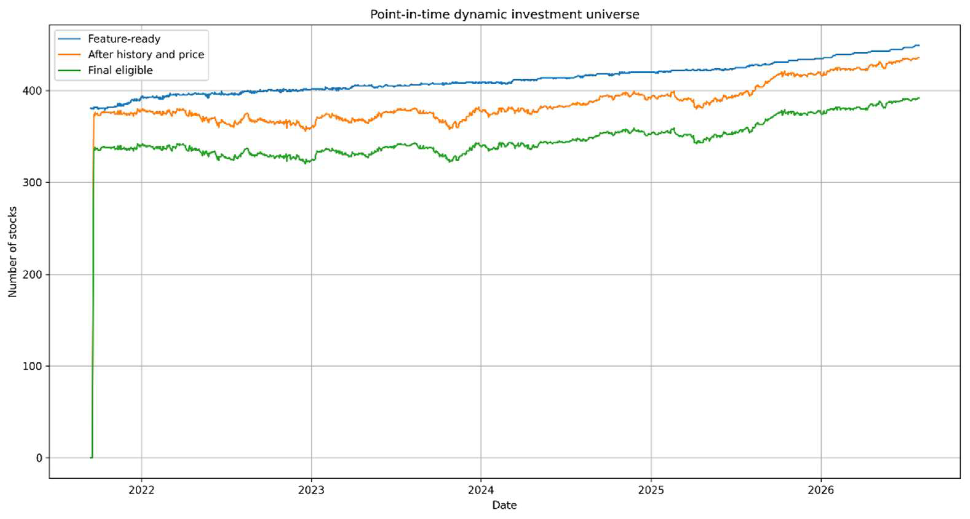
Figure A2.
Time-varying liquidity threshold.
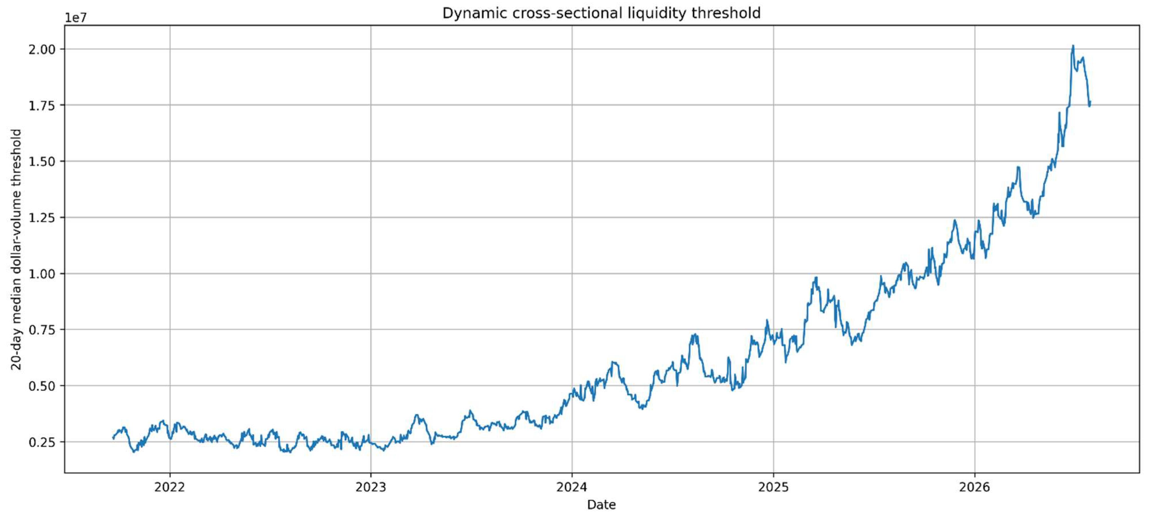
Table A1.
Sensitivity of the dynamic investment universe to alternative screening rules.
Table A2.
Newey–West lag sensitivity for selected main strategies.
Figure A3.
Liquidity-gated annual geometric returns.
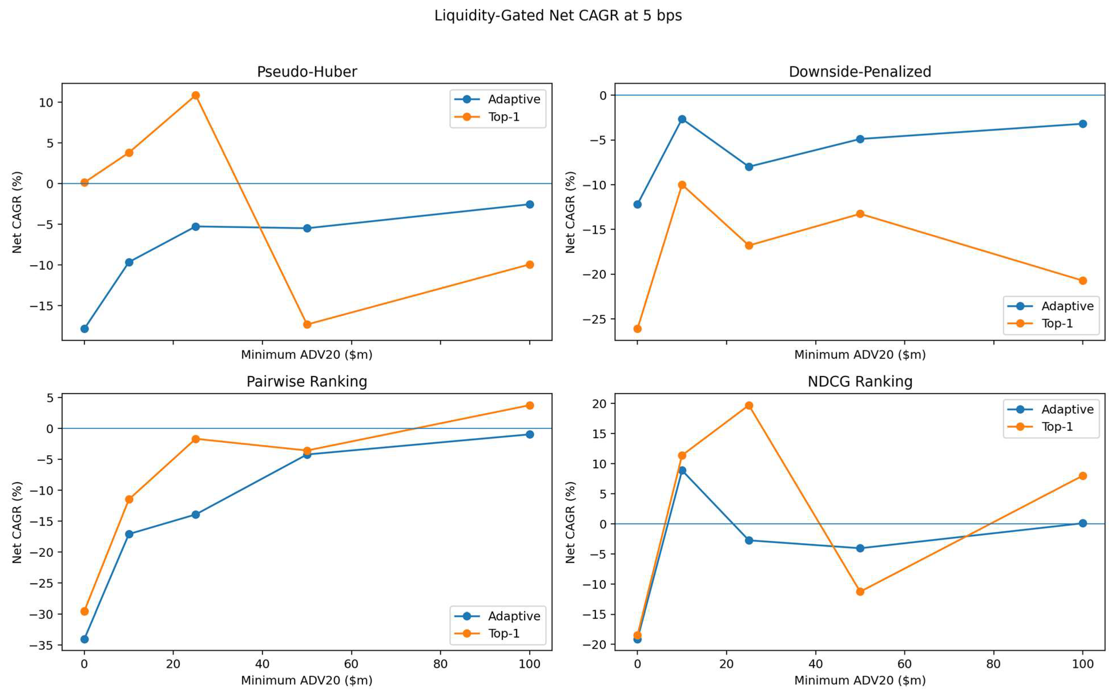
References
- Amihud, Y. (2002). Illiquidity and stock returns: Cross-section and time-series effects. Journal of Financial Markets, 5(1), 31–56. [Google Scholar] [CrossRef] [Scilit]
- Anghel, D. G. (2021). Data snooping bias in tests of the relative performance of multiple forecasting models. Journal of Banking & Finance, 126, 106113. [Google Scholar] [CrossRef] [Scilit]
- Bailey, D. H., Borwein, J. M., López de Prado, M., & Zhu, Q. J. (2014). Pseudo-mathematics and financial charlatanism: The effects of backtest overfitting on out-of-sample performance. Notices of the American Mathematical Society, 61(5), 458–471. Available online: https://www.ams.org/notices/201405/rnoti-p458.pdf (accessed on 26 August 2026). [CrossRef] [Scilit]
- Bergmeir, C., & Benitez, J. M. (2012). On the use of cross-validation for time series predictor evaluation. Information Sciences, 191, 192–213. [Google Scholar] [CrossRef] [Scilit]
- Brock, W., Lakonishok, J., & LeBaron, B. (1992). Simple technical trading rules and the stochastic properties of stock returns. Journal of Finance, 47(5), 1731–1764. [Google Scholar] [CrossRef]
- Burges, C. J. C. (2010). From RankNet to LambdaRank to LambdaMART: An overview. Microsoft research technical report. Available online: https://www.microsoft.com/en-us/research/publication/from-ranknet-to-lambdarank-to-lambdamart-an-overview/ (accessed on 26 August 2026).
- Burges, C. J. C., Shaked, T., Renshaw, E., Lazier, A., Deeds, M., Hamilton, N., & Hullender, G. (2005). Learning to rank using gradient descent. In Proceedings of the 22nd international conference on machine learning (pp. 89–96). Association for Computing Machinery. Available online: https://icml.cc/Conferences/2005/proceedings/papers/012_LearningToRank_BurgesEtAl.pdf (accessed on 26 August 2026).
- Cerqueira, V., Torgo, L., & Mozetic, I. (2020). Evaluating time series forecasting models: An empirical study on performance estimation methods. Machine Learning, 109(11), 1997–2028. [Google Scholar] [CrossRef] [Scilit]
- Chen, A. Y., & Zimmermann, T. (2022). Open source cross-sectional asset pricing. Critical Finance Review, 11(2), 207–264. [Google Scholar] [CrossRef] [Scilit]
- Chen, T., & Guestrin, C. (2016). XGBoost: A scalable tree boosting system. In Proceedings of the 22nd ACM SIGKDD international conference on knowledge discovery and data mining (pp. 785–794). Association for Computing Machinery. [Google Scholar] [CrossRef] [Scilit]
- DeMiguel, V., Martin-Utrera, A., Nogales, F. J., & Uppal, R. (2020). A transaction-cost perspective on the multitude of firm characteristics. Review of Financial Studies, 33(5), 2180–2222. [Google Scholar] [CrossRef] [Scilit]
- Fieberg, C., Metko, D., Poddig, T., & Loy, T. (2023). Machine learning techniques for cross-sectional equity returns’ prediction. OR Spectrum, 45, 289–323. [Google Scholar] [CrossRef] [Scilit]
- Freyberger, J., Neuhierl, A., & Weber, M. (2020). Dissecting characteristics nonparametrically. Review of Financial Studies, 33(5), 2326–2377. [Google Scholar] [CrossRef] [Scilit]
- Friedman, J. H. (2001). Greedy function approximation: A gradient boosting machine. Annals of Statistics, 29(5), 1189–1232. [Google Scholar] [CrossRef] [Scilit]
- Gu, S., Kelly, B., & Xiu, D. (2020). Empirical asset pricing via machine learning. Review of Financial Studies, 33(5), 2223–2273. [Google Scholar] [CrossRef] [Scilit]
- Hampel, F. R., Ronchetti, E. M., Rousseeuw, P. J., & Stahel, W. A. (1986). Robust statistics: The approach based on influence functions. Wiley. [Google Scholar] [CrossRef] [Scilit]
- Harvey, C. R., Liu, Y., & Zhu, H. (2016). … and the cross-section of expected returns. Review of Financial Studies, 29(1), 5–68. [Google Scholar] [CrossRef] [Scilit]
- Huber, P. J. (1964). Robust estimation of a location parameter. Annals of Mathematical Statistics, 35(1), 73–101. [Google Scholar] [CrossRef] [Scilit]
- Jensen, T. I., Kelly, B., Malamud, S., & Pedersen, L. H. (2026). Machine learning and the implementable efficient frontier. Review of Financial Studies, hhag022. [Google Scholar] [CrossRef] [Scilit]
- Korajczyk, R. A., & Sadka, R. (2004). Are momentum profits robust to trading costs? Journal of Finance, 59(3), 1039–1082. [Google Scholar] [CrossRef] [Scilit]
- Kottas, F. (2026). A hybrid genetic algorithm with learning-to-rank-to-optimization for US equity portfolio construction. International Journal of Financial Studies, 14(4), 95. [Google Scholar] [CrossRef] [Scilit]
- Kozak, S., Nagel, S., & Santosh, S. (2020). Shrinking the cross-section. Journal of Financial Economics, 135(2), 271–292. [Google Scholar] [CrossRef] [Scilit]
- Leippold, M., Wang, Q., & Zhou, W. (2022). Machine learning in the Chinese stock market. Journal of Financial Economics, 145(2), 64–82. [Google Scholar] [CrossRef] [Scilit]
- Li, S., Mulvey, J. M., & Fabozzi, F. J. (2026). Smart trading rule: A modular machine learning framework for portfolio optimization with transaction costs. Journal of Financial Data Science, 8(2), 145–175. [Google Scholar] [CrossRef] [Scilit]
- Liu, T.-Y. (2009). Learning to rank for information retrieval. Foundations and Trends in Information Retrieval, 3(3), 225–331. [Google Scholar] [CrossRef] [Scilit]
- Lo, A. W., Mamaysky, H., & Wang, J. (2000). Foundations of technical analysis: Computational algorithms, statistical inference, and empirical implementation. Journal of Finance, 55(4), 1705–1765. [Google Scholar] [CrossRef] [Scilit]
- López de Prado, M. (2018). Advances in financial machine learning. Wiley. [Google Scholar]
- McLean, R. D., & Pontiff, J. (2016). Does academic research destroy stock return predictability? Journal of Finance, 71(1), 5–32. [Google Scholar] [CrossRef] [Scilit]
- Neely, C. J., Rapach, D. E., Tu, J., & Zhou, G. (2014). Forecasting the equity risk premium: The role of technical indicators. Management Science, 60(7), 1772–1791. [Google Scholar] [CrossRef] [Scilit]
- Novy-Marx, R., & Velikov, M. (2016). A taxonomy of anomalies and their trading costs. Review of Financial Studies, 29(1), 104–147. [Google Scholar] [CrossRef] [Scilit]
- Patton, A. J., & Weller, B. M. (2020). What you see is not what you get: The costs of trading market anomalies. Journal of Financial Economics, 137(2), 515–549. [Google Scholar] [CrossRef] [Scilit]
- Poh, D., Lim, B., Zohren, S., & Roberts, S. (2021). Building cross-sectional systematic strategies by learning to rank. Journal of Financial Data Science, 3(2), 70–86. [Google Scholar] [CrossRef] [Scilit]
- Safari, M., Nakharutai, N., Chiawkhun, P., & Phetpradap, P. (2025). Dynamic portfolio optimization: A two-stage hybrid approach integrating selection and allocation. Risk and Decision Analysis, 12(1), 49–64. [Google Scholar] [CrossRef] [Scilit]
- Shumway, T. (1997). The delisting bias in CRSP data. Journal of Finance, 52(1), 327–340. [Google Scholar] [CrossRef]
- Song, Q., Liu, A., & Yang, S. Y. (2017). Stock portfolio selection using learning-to-rank algorithms with news sentiment. Neurocomputing, 264, 20–28. [Google Scholar] [CrossRef] [Scilit]
- Sullivan, R., Timmermann, A., & White, H. (1999). Data-snooping, technical trading rule performance, and the bootstrap. Journal of Finance, 54(5), 1647–1691. [Google Scholar] [CrossRef] [Scilit]
- Tashman, L. J. (2000). Out-of-sample tests of forecasting accuracy: An analysis and review. International Journal of Forecasting, 16(4), 437–450. [Google Scholar] [CrossRef] [Scilit]
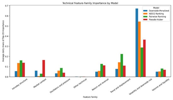
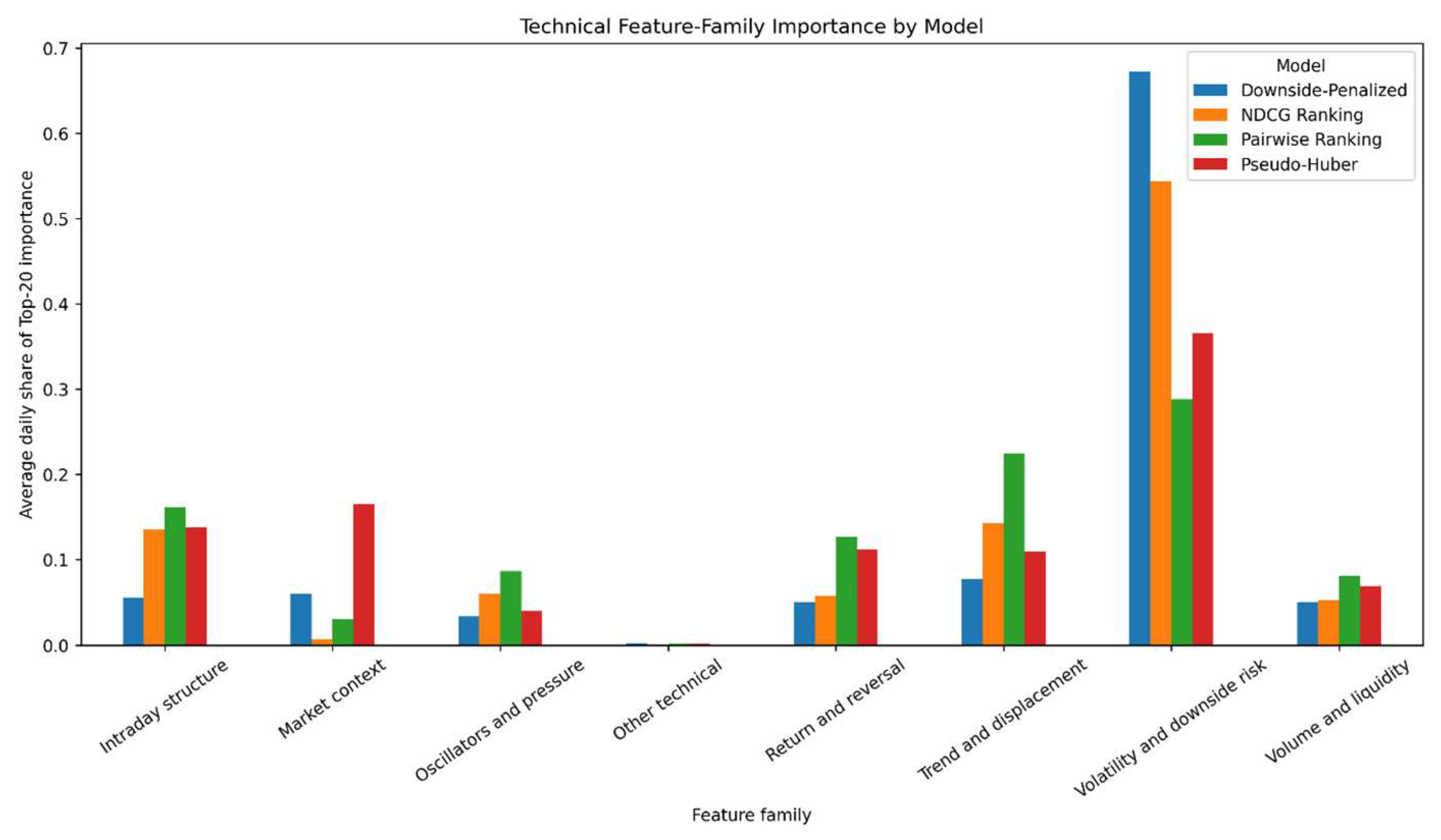
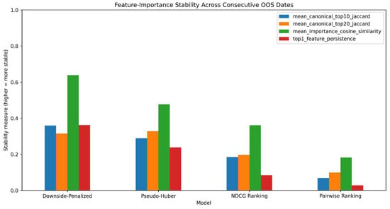
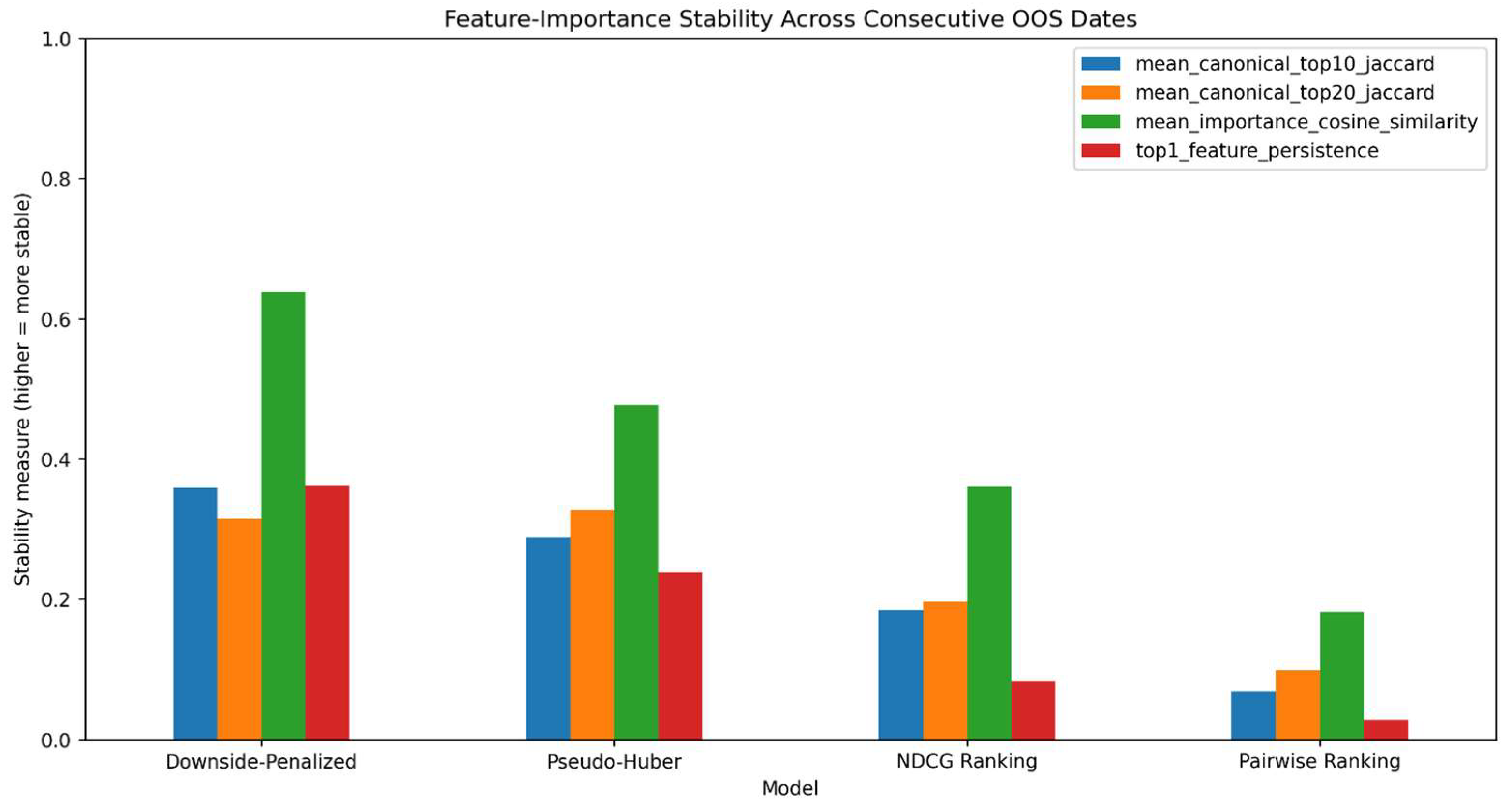
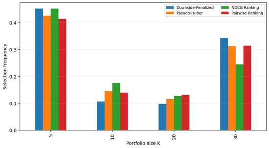
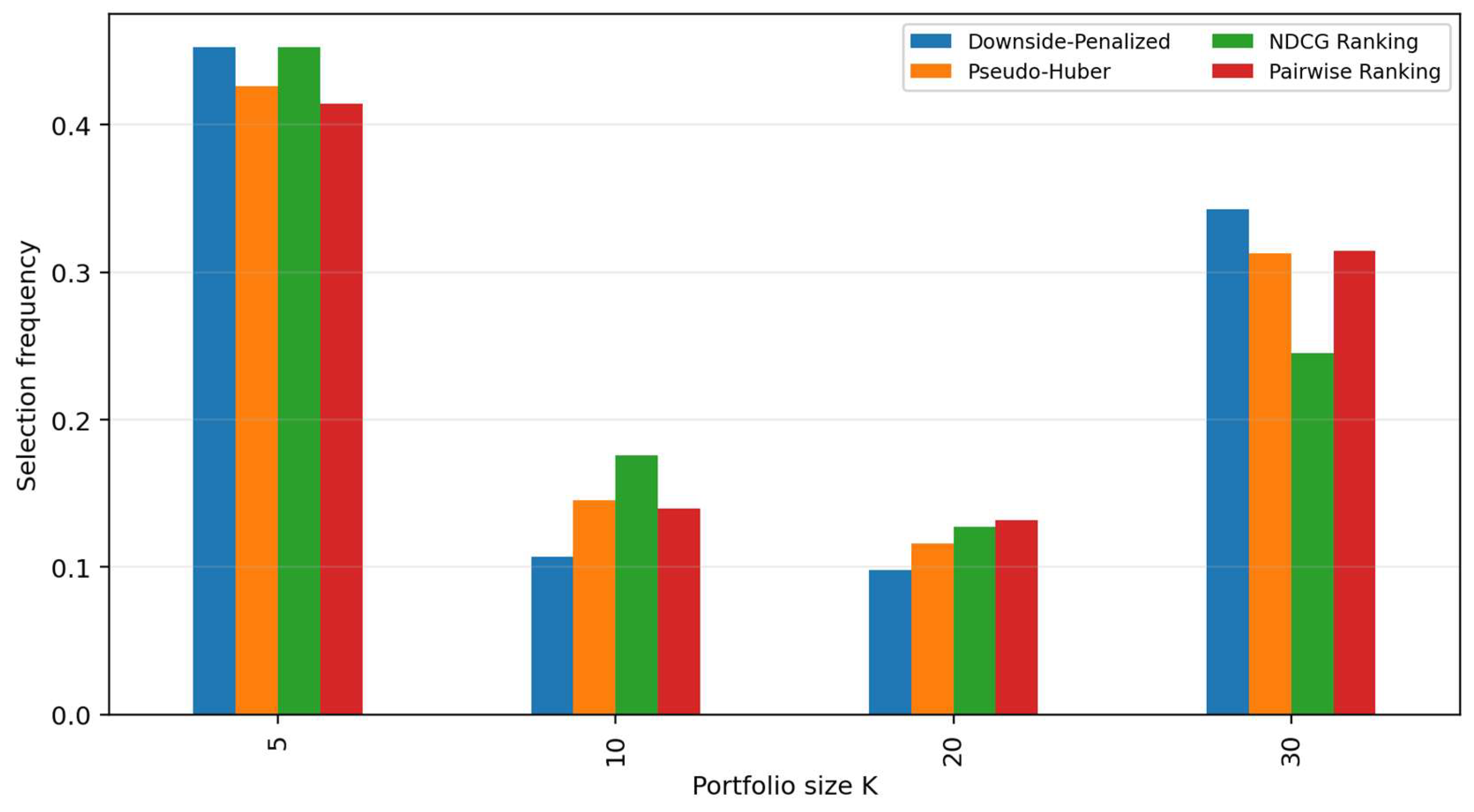
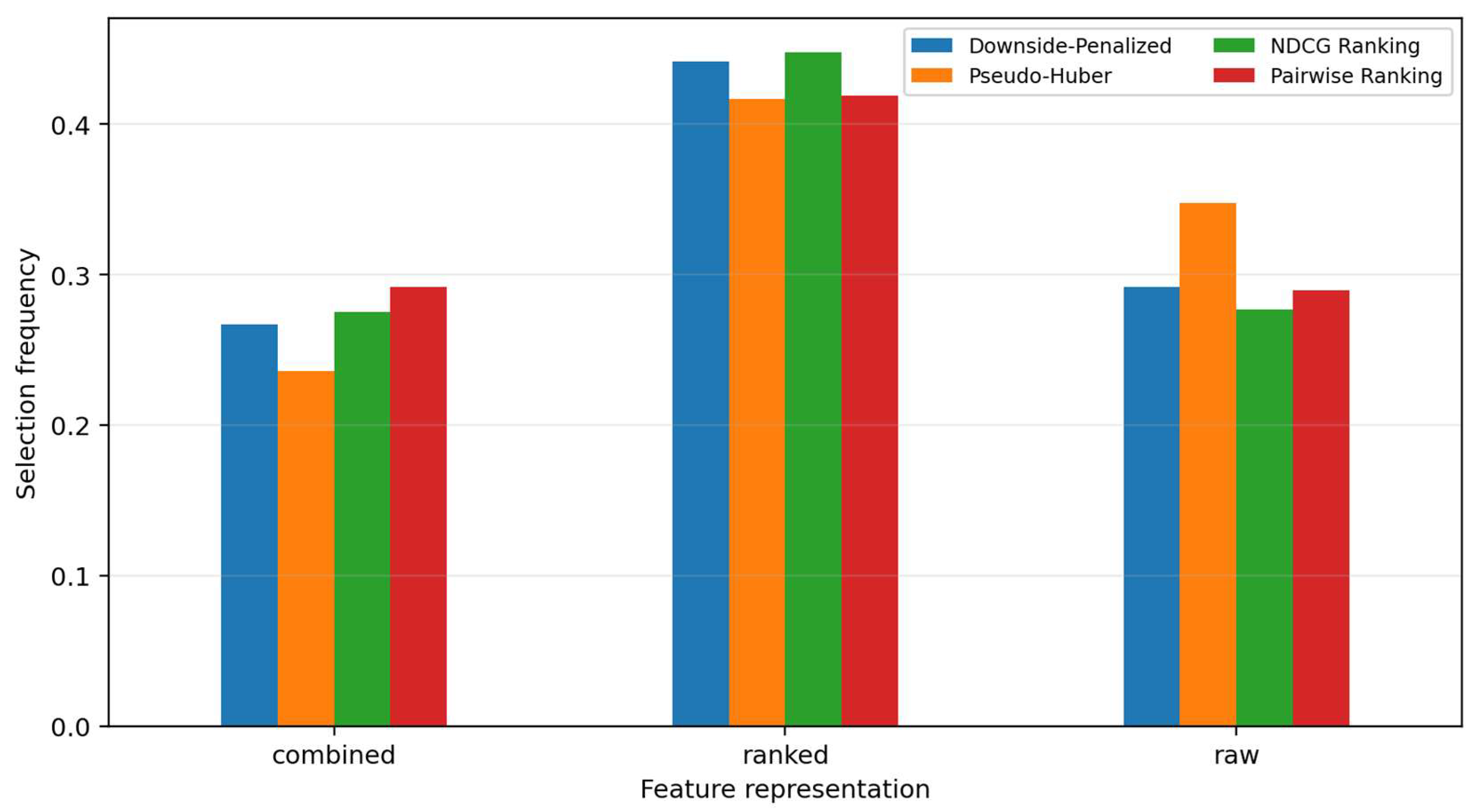
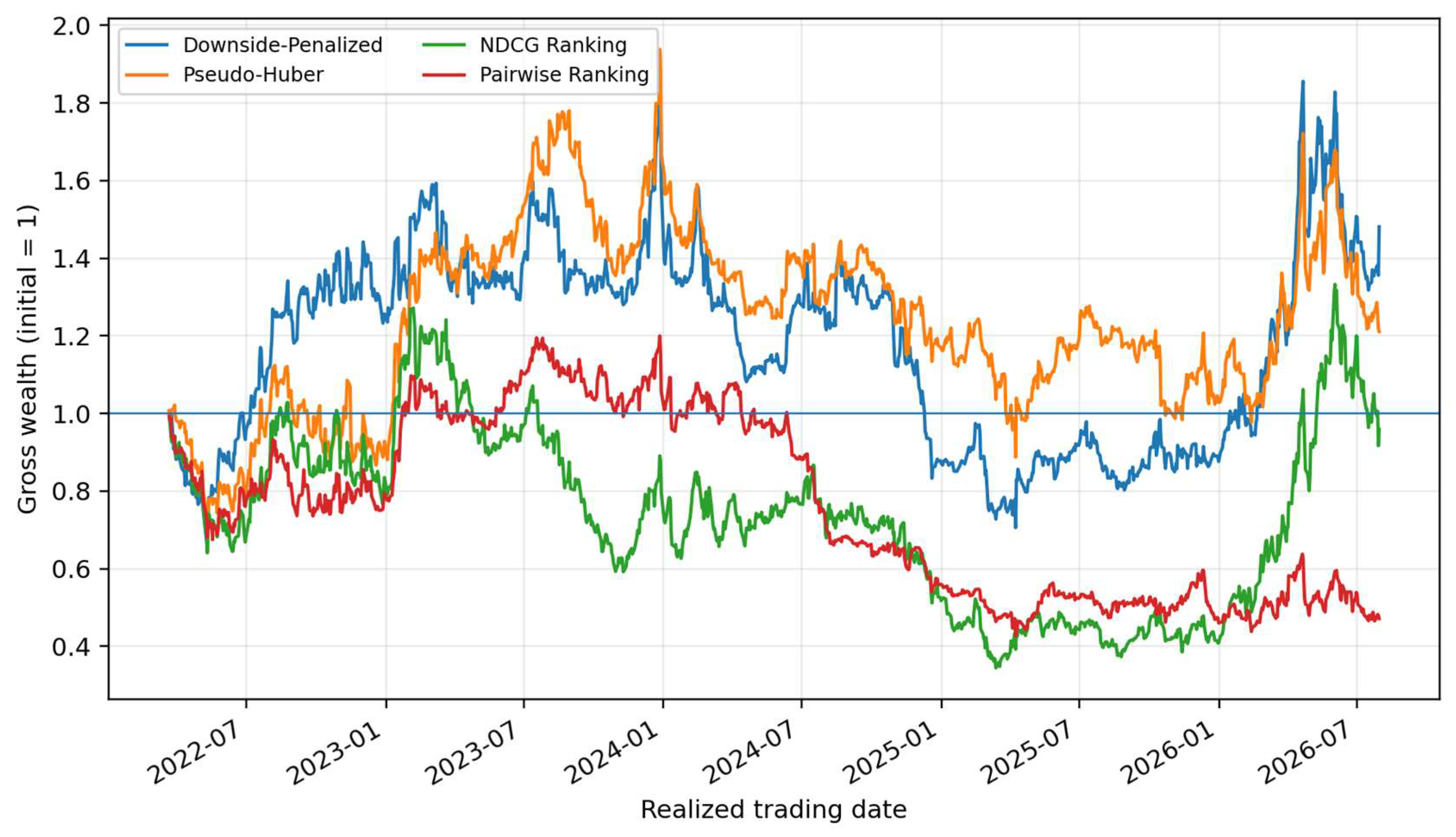
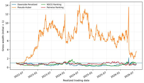
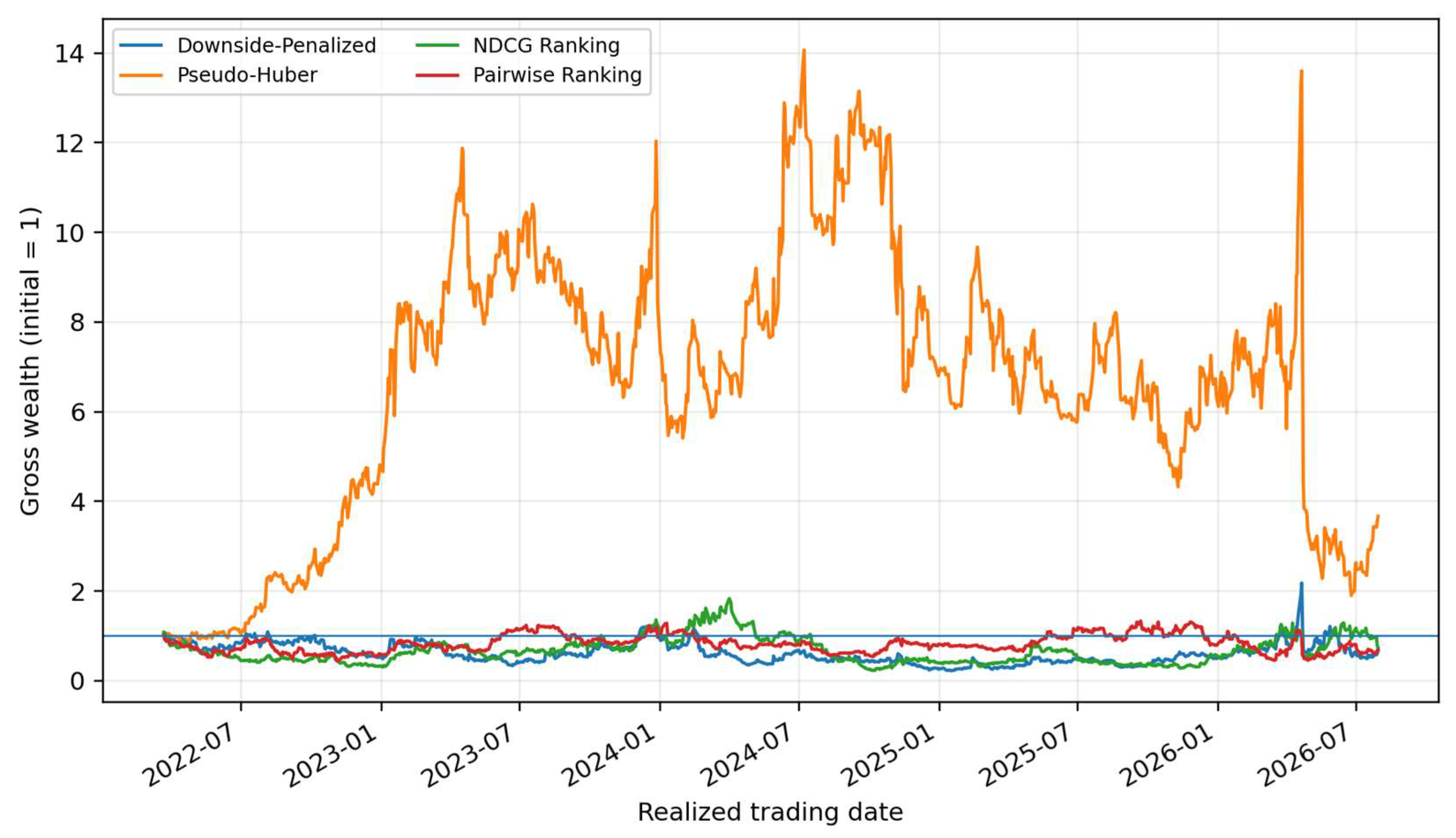
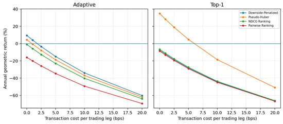
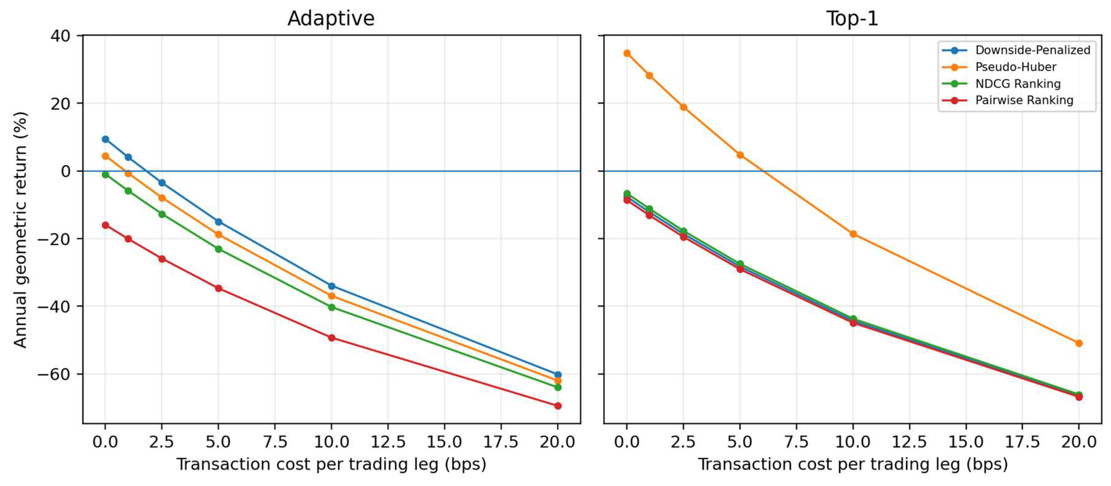
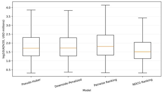
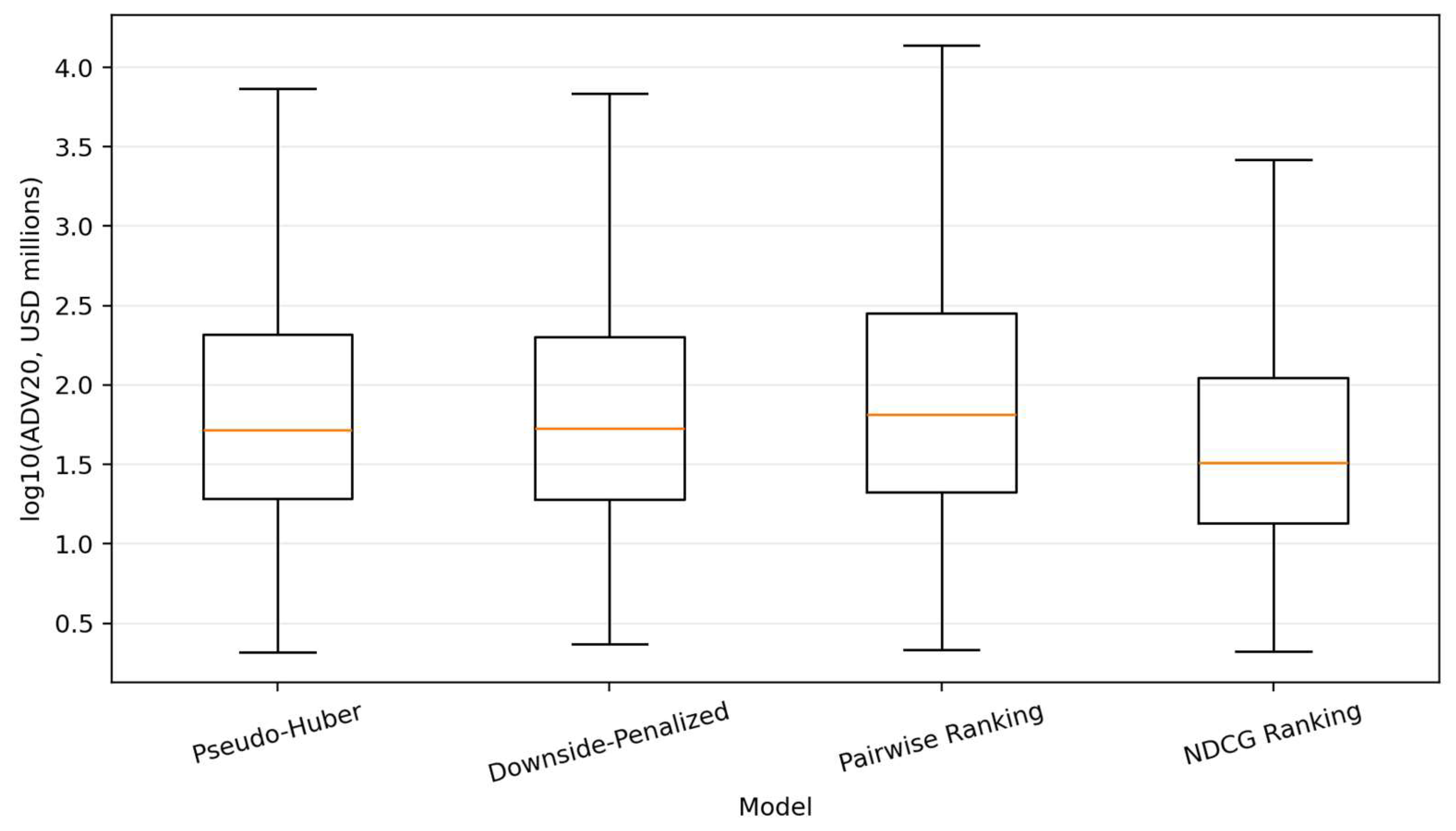
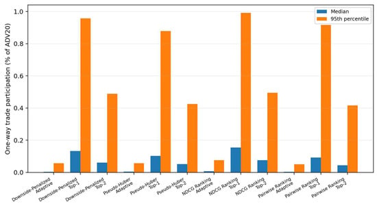
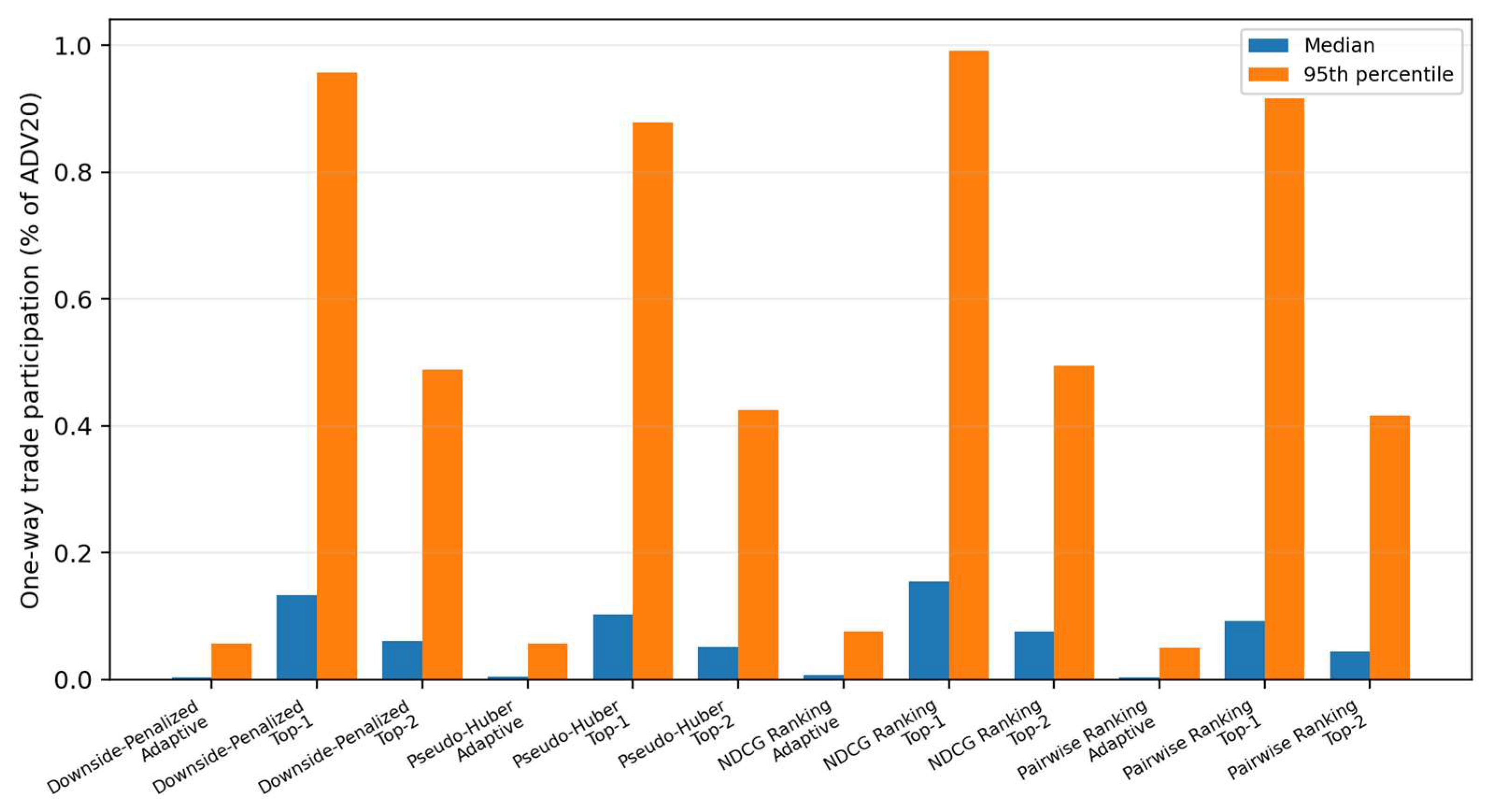

Disclaimer/Publisher’s Note: The statements, opinions and data contained in all publications are solely those of the individual author(s) and contributor(s) and not of MDPI and/or the editor(s). MDPI and/or the editor(s) disclaim responsibility for any injury to people or property resulting from any ideas, methods, instructions or products referred to in the content. |
© 2026 by the author. Licensee MDPI, Basel, Switzerland. This article is an open access article distributed under the terms and conditions of the Creative Commons Attribution (CC BY) license.