


Abstract
This paper examines how Croatia’s transition from monetary sovereignty to euro adoption reshaped the structure of inflation transmission between 2000 and 2025. The analysis employs a two-stage empirical framework grounded in Modern Monetary Theory (MMT). In the first stage, the study tests the Decoupling Axiom through a Panel ARDL model across Croatia and comparable CEE economies, finding that pre-euro policy interest rates were governed by their own inertia rather than by the fiscal stance—evidence of functional monetary sovereignty—while the sovereign-yield evidence indicates that markets price the fiscal flow (the deficit) but not the accumulated debt stock. In the second stage, a Hybrid Bayesian Structural Time Series (BSTS) model constructs model-based counterfactuals to estimate the association between euro adoption and sectoral inflation dynamics. The results reveal a sharp, treatment-timed cooling of new-housing inflation relative to consumption and services, concentrated at the 2023 adoption date and fading substantially by 2025—a shock-and-fade pulse rather than a permanent realignment. Falsification tests and a Causal Impact prior-sensitivity check support this reading, while a Generalized Synthetic Control, which rebuilds the counterfactual from an actual donor pool, does not reproduce the aggregate sign-asymmetry: what survives as genuinely cross-method is a narrower durables-versus-services divergence, anchored by the computer-versus-hotels spread inflation and reinforced by a furnishings-based contrast. Because inference rests on only three post-adoption years coinciding with the post-pandemic inflation surge, the energy shock, and ECB tightening, the design cannot fully isolate the currency changeover from contemporaneous disturbances. The findings should therefore be read as consistent with, rather than as conclusive proof of, MMT’s prediction of a sectoral reconfiguration of inflation under a shared monetary regime.
Keywords:
monetary sovereignty; MMT; BSTS; Causal Impact; Gsynth; euro adoption; Croatia; inflation transmission 1. Introduction
The introduction of the euro marked a fundamental transformation in the institutional architecture of European monetary governance. For small open economies such as Croatia, the euro adoption entailed not only a nominal currency change but a structural redefinition of macroeconomic sovereignty. Under sovereign monetary regimes, fiscal and monetary authorities retain the capacity to coordinate liquidity management, debt issuance, and domestic stabilization. By contrast, euro adoption substitutes domestic discretion with external anchoring—monetary policy becomes exogenous, and inflation transmission mechanisms are reshaped by supranational financial and policy structures.
Within the state institutional framework, Croatia’s 2023 accession to the euro monetary area constitutes a pivotal milestone in its long trajectory of monetary integration. Although the transition enhanced the institutional credibility and stability, and eliminated exchange rate risks, it simultaneously constrained the country capacity for autonomous macroeconomic adjustment. This trade-off reflects a structural problem of vulnerability long observed in the eurozone peripheral members. Earlier studies suggest that monetary convergence amplifies asymmetric shocks (Honohan & Lane, 2003), constrain fiscal responsiveness (Nenovsky, 2020), and foster core–periphery inflation divergence (Gibson et al., 2014). These dynamics are particularly relevant for small economies where domestic sterilization capacity and credit multipliers are structurally limited.
Modern Monetary Theory (MMT) provides a conceptual framework for interpreting these transformations. Rather than defining monetary sovereignty solely in terms of the legal authority to issue a national currency, MMT conceptualizes it as the state’s institutional capacity to issue, tax, and regulate it (Wray, 2012; Kelton, 2020). Within this framework, inflation reflects the interaction between fiscal capacity, productive constraints, and institutional autonomy. Once monetary authority is surrendered, as through euro adoption, a country loses its ability to sterilize liquidity or offset external shocks through endogenous policy coordination. Inflation then ceases to be a domestic variable—it becomes a derivative of cross-border financial flows and imported cost structures.
Croatia’s post-2021 inflation trajectory provides an illustrative case of this institutional transition. The initial surge, driven by pandemic-related supply disruptions (2021), energy shocks (2022), and government-mandated wage adjustments (CBS; Croatian Bureau of Statistics, 2022), was structurally amplified by euro adoption. However, these transitory factors elevated prices temporarily, while the currency transition produced a deeper regime shift: a rechanneling of inflation pressure from asset-based to consumption-based sectors. This dynamic validates MMT’s prediction that monetary integration redistributes inflationary burdens toward consumption goods and household demand (Wray, 2015; Cesaratto, 2015, Zimmermann, 2014).
Empirically, this study employs a two-stage framework. The first stage tests the Decoupling Axiom: the proposition that sovereign monetary systems exhibit independence between fiscal stance and policy interest rates using a Panel ARDL model across Croatia and comparable CEEs (Central European Economies). The second stage applies a Hybrid Bayesian Structural Time Series (BSTS) model, validated through Causal Impact and Generalized Synthetic Control (Gsynth) frameworks, to identify how the loss of monetary sovereignty reshaped inflation transmission following euro adoption.
The empirical findings indicate a marked inversion in inflation dynamics: asset-based price growth, particularly in new housing and investment categories, contracted after euro adoption, while consumption-related inflation accelerated. This emergent reallocation of inflationary pressure points to an early-stage transition of inflation from a policy-anchored toward a more market-driven process, consistent with MMT’s theoretical proposition that the erosion of monetary sovereignty redefines both the composition and propagation of price dynamics.
This paper makes three contributions. First, whereas the Modern Monetary Theory literature characterizes monetary sovereignty largely in conceptual or narrative terms (Wray, 2012, 2015; Kelton, 2020), we provide a formal, falsifiable test of its central Decoupling Axiom—the proposed independence of the policy interest rate from the fiscal stance—using a Panel ARDL framework across Croatia and comparable CEE economies. Second, in contrast to the euro-area inflation literature, which typically evaluates convergence at the level of aggregate or headline inflation (Honohan & Lane, 2003; Gibson et al., 2014; Lane, 2023), we exploit recent counterfactual machinery (BSTS, Causal Impact, Gsynth) to measure the effect of a currency-regime switch at the sectoral level, documenting a redistribution of price pressure from asset-based toward consumption-based channels that aggregate measures conceal. Third, Croatia’s 2023 accession offers the most recent and institutionally cleanest euro-adoption episode available, providing fresh evidence for the core–periphery and critical macro-finance debates on how hierarchical liquidity structures (Gabor, 2021) and persistent structural asymmetries (Stiglitz, 2016) condition inflation in small open economies.
This paper bridges theoretical and empirical perspectives on monetary integration, suggesting how the euro’s stabilizing credibility coexists with the structural weakening of domestic transmission autonomy. The results have broader implications for understanding inflation asymmetries in peripheral Eurozone members and for evaluating the policy trade-offs between nominal stability, fiscal flexibility, and inflation resilience.
The remainder of the paper is organized as follows. Section 2 reviews the theoretical and methodological literature on monetary sovereignty and inflation transmission. Section 3 describes the data and the two-stage empirical framework. Section 4 sets out the Panel ARDL stage, and Section 5 reports the results—the model framework and preliminary diagnostics, cointegration and the error-correction evidence, the optimal ARDL estimation on the preferred instrument, and the short-rate robustness analysis—together with the Hybrid BSTS stage, its placebo testing, and the Causal Impact and Gsynth validation. Section 6 discusses the findings in light of the MMT framework, and Section 7 concludes.
2. Literature Review
The literature on monetary sovereignty and inflation transmission has evolved through two distinct paradigms. Traditional models, rooted in New Keynesian and DSGE frameworks, emphasize price stability as a function of nominal anchors and external credibility (Blanchard & Galí, 2007; Clarida et al., 1999).
Within this paradigm, monetary integration enhances macroeconomic stability by eliminating the exchange rate uncertainty, strengthening policy credibility and constraining inflationary bias through a common monetary authority. These models view monetary integration as a stabilizing mechanism that disciplines fiscal policy and anchors expectations. More recent findings (Blanchard & Pisani-Ferry, 2022; Borio et al., 2019) highlighted the post-pandemic inflation dynamics in the eurozone, and exposed the fragility of this framework, demonstrating that credibility-based stabilization can coexist with persistent structural asymmetries.
However, recent distinct paradigms, particularly from the Modern Monetary Theory (MMT) provide an alternative perspective, disputing that integration erodes domestic policy autonomy and redistributes inflationary pressure across sectors (Wray, 2015; Kelton, 2020). Within the MMT framework, inflation reflects the interaction between fiscal capacity, productive constraints, and institutional sovereignty. Empirical studies on post-sovereignty regimes show that the loss of currency control often shifts inflation transmission from asset and investment channels toward consumer and import-dependent sectors (Goodhart & Pradhan, 2020; Cesaratto, 2015). Complementing this perspective, critical macro-financial approaches emphasize that euro-area integration embeds hierarchical liquidity structures, limiting peripheral states’ ability to manage domestic credit cycles and price formation (Gabor, 2021).
This realignment implies that monetary integration stabilizes expectations but weakens the internal capacity to absorb liquidity shocks, especially in small open economies. Lane (2023) further shows that persistent productivity differentials and supply-side rigidities within the Eurozone continue to generate asymmetric inflation responses despite common monetary conditions, reinforcing MMT’s claim that structural divergence endures beyond nominal convergence.
Complementary arguments have been advanced by Stiglitz (2016), who, from a neo-Keynesian standpoint, highlights the structural unsustainability of the euro project arising from persistent productivity and fiscal asymmetries across member states. According to these arguments, the absence of a fiscal union and limited adjustment mechanisms amplify cyclical divergence and constrain national responses to inflationary pressures. Furthermore, Stiglitz’s critique aligns with MMT insights: both suggest that the erosion of monetary sovereignty reduces macroeconomic flexibility and exposes peripheral economies to externally transmitted inflation dynamics.
Parallel methodological developments have substantially expanded the toolkit for analyzing such regime shifts and institutional transitions. The Bayesian Structural Time Series (BSTS) framework (Scott & Varian, 2014) enables causal inference in the presence of latent structural components, while the Causal Impact extension (Brodersen et al., 2015) and Generalized Synthetic Control (Xu, 2017) approaches enhance counterfactual credibility in policy evaluation. Recent advances in macroeconometric modeling, such as high-dimensional dynamic factor structures (Bańbura & Modugno, 2014) and refined Bayesian convergence diagnostics (Vehtari et al., 2021), have strengthened the empirical reliability of hierarchical and synthetic inference methods, allowing for robust estimation of policy effects in small samples. Applied to the euro context, these methods permit the decomposition of inflation responses into structural, sectoral, and regime-specific effects.
Building on these theoretical and methodological foundations, this study applies a two-stage empirical framework to the Croatian case, using the Modern Monetary Theory (MMT) perspective as an interpretive lens for understanding how the loss of currency sovereignty reconfigures inflation transmission under euro adoption.
3. Theoretical Framework
Croatia’s adoption of the euro in 2023 marked not merely the completion of Croatia’s monetary integration into the eurozone, it marked an institutional transition with potentially important implications for the mechanisms through which inflation is generated and transmitted. Within the perspective of Modern Monetary Theory (MMT), this change can be interpreted as an early-stage transition from a sovereignly managed system, where the state could channel inflation between asset and consumer sectors toward an externally anchored regime where such discretion is lost (Wray, 2012).
A conceptual clarification is necessary before proceeding. The study distinguishes formal (de jure) monetary sovereignty, legal control over an independent currency and the associated policy instruments, which Croatia retained until 2023 from functional sovereignty, and the de facto capacity to exercise autonomous monetary policy. The latter was already materially constrained well before euro adoption: the kuna operated under a tightly managed exchange-rate regime, and deposits accounted approximately 80% of the banking system, leaving the central bank with limited space for genuinely independent actions. Consequently, our analysis therefore concerns the loss of the residual functional autonomy “sterilization capacity” that the CNB still commanded under the sovereign kuna regime, rather than a transition from full monetary sovereignty to none. The pre/post contrast we document is accordingly one of degree rather than kind, and, as we argue below, this is precisely what renders the already heavily euroized CEE economies appropriate counterfactual units (see Section 4.4).
3.1. Dual Inflation Channels Under Croatian Sovereign Monetary Conditions
During the sovereign kuna regime, Croatia exhibited a dual-channel inflation structure, reflecting deliberate monetary management consistent with MMT’s notion of functional sovereignty. The Croatian National Bank (CNB) maintained control over liquidity through sterilized interventions, which enabled selective inflation channeling between asset markets and the consumer economy.
- Asset-based inflation channel: inflation pressures were directed primarily into asset-intensive sectors, notably new housing and real estate, where capital absorption acted as a stabilizer for broader price levels. This process reflected a quasi-Keynesian use of asset inflation as a containment mechanism for excess liquidity (Palley, 2013), whereby monetary authorities deliberately redirected inflationary pressures toward real estate markets—transforming housing into a “liquidity sink” that partially absorbed excess liquidity, without generating proportionate increases in consumer prices and collateral-driven demand. The resulting appreciation in real estate values benefited asset holders, developers, and foreign investors, while leaving consumer price inflation relatively subdued.
- Consumption-based inflation channel: inflation in everyday goods, i.e., food, transport, and utilities, remained stable due to the CNB’s sterilization of tourism-driven forex inflows, a mechanism that functioned as a liquidity tax (Wray, 2012; Bell, 2000). By issuing domestic bonds to absorb excess kuna liquidity, the CNB directed monetary contraction disproportionately toward consumption channels, compressing household purchasing power while asset-market liquidity remained comparatively insulated (Reinhart & Reinhart, 2011). This asymmetric containment explains the divergence between Croatia’s soaring real estate prices and subdued CPI.
This two-tiered structure demonstrates MMT’s core claim: under sovereign conditions, inflation can be distributed rather than uniformly transmitted. The capacity to direct inflation into asset markets, while insulating consumer prices, sustained social and macroeconomic stability at the cost of rising wealth inequality (for formal expressions of this framework, see Appendix A: Formal MMT Transmission Framework).
3.2. Croatian Regime Transition: From Sovereign Control to Euro Externalization
Croatia’s adoption of the euro in 2023 fundamentally altered monetary structure by surrendering control over interest rates, exchange interventions, and sterilization mechanisms. As De Grauwe (2020) accentuates, joining a monetary union entails the irreversible loss of national monetary policy instruments, binding members to a one size fits all framework, an aggregate monetary space within which peripheral economies like Croatia face even less autonomy than certain U.S. states. Consequently, Croatia now faces liquidity and inflation dynamics externally determined by the European Central Bank (ECB), with reduced monetary sovereignty and constrained monetary and fiscal autonomy. The transition can be characterized as “the abandonment of functional sovereignty in inflation management” Wray (2012, p. 189). This emerging shift exposes Croatia to the ECB’s policy priorities, which may misalign with domestic economic conditions, as evidenced by divergent inflation trajectories across small eurozone economies (Honohan & Lane, 2003; Gibson et al., 2014).
The Croatian monetary transition framework consists of three key outcomes:
- Loss of monetary sovereignty: membership in the euro area eliminates the CNB capability to conduct sterilization of euro inflows, leading to direct liquidity injection into the domestic economy. As a result, this exposes households to higher consumption-based inflation as euros circulate unmediated through demand channels.
- Persistence: transformation of asset inflation: asset markets, particularly residential real estates (houses), continue to benefit due to eurozone credit integration and cross-border portfolio flows. Yet, without autonomous policy instruments, these inflows cannot be offset domestically, turning real estate (housing) into a speculative rather than stabilizing channel.
- Emerging spread divergence: the inflation spread (Spread(A − C) = π(Assets) − π(Consumables)) shifts from near-zero/positive under sovereign conditions (where targeted sterilization contained ) to decisively negative post-euro. This reversal reflects MMT’s prediction that currency unions force inflation convergence onto consumption baskets via unmediated liquidity injection (Wray, 2012; Bell, 2000), a pattern empirically observed in Eurozone periphery economies where outpaces by 2–5 pp (Honohan & Lane, 2003; Gibson et al., 2014).
Taken together, this framework suggests a financialization of inflation transmission: rather than channeling excess liquidity into asset buffers, the system now amplifies consumption volatility while asset inflation persists at high but uneven levels.
3.3. Distributional and Structural Implications
The institutional changes associated with the euro adoption also have important distributional implications, by altering the sectoral incidence and the allocation of adjustment costs. From the MMT perspective, the changes in the mechanisms of inflation transmission are not equally distributed; they altered inflation dynamics across different socioeconomic population groups, redistributing losses to middle- and low-income households while entrenching gains for asset holders.
During the sovereign kuna regime, the sterilization policies shielded consumers (Stiglitz, 2016, p. 213), largely protecting low-/middle-income households from essentials inflation, while deliberate liquidity channeling enriched asset holders through managed real estate and equity appreciation (Piketty, 2014, p. 335).
Under these conditions, in the post-euro period, unmediated liquidity floods consumption channels impoverished households unevenly, via uncontained inflation in essential consumption categories, i.e., food and utilities, (Fitoussi & Saraceno, 2010). Simultaneously, asset holders captured gains from speculative capital inflows, now detached from stabilization logic, deepening wealth inequality (Stockhammer, 2015).
During the Croatian shift from functional monetary sovereignty toward non-sovereign EU monetary policy, in relative terms, asset holders were comparatively better insulated and positioned to absorb inflation shocks, while the households with average incomes took over the greater adjustment of the burden. Consistent with the arguments of Blyth (2013, p. 76), the imposed euro membership and loss of monetary autonomy reduces states to “rule-takers”, redistributing inflation burdens to the socially vulnerable. Croatia’s inflation now mirrors external governance, its transmission channels structurally favoring capital over labor (Wray, 2012, p. 204), thereby amplifying social transmission asymmetries: around one-fifth of the population remains at risk of poverty or social exclusion, and over a third of those aged 65+ face the same risk (Croatian Bureau of Statistics, 2024).
4. Materials and Methods—The Methodological Design and Data Framework
The methodological design of this study is structured to examine empirically whether the surrender of monetary sovereignty, exemplified by Croatia’s 2023 euro adoption, has altered the mechanisms through which inflation and asset prices interact. The analysis follows the logic of Modern Monetary Theory (MMT), in which the capacity to direct inflation through distinct channels depends on the institutional autonomy of the monetary authority.
To situate this framework for readers less accustomed to the MMT literature, it is worth noting where its predictions converge with, and diverge from, those of conventional New Keynesian (NK) and DSGE models. Both traditions agree that relinquishing an independent monetary instrument alters inflation dynamics: in the open-economy NK tradition (Galí & Monacelli, 2005; Farhi & Werning, 2019), a country that abandons autonomous interest-rate and exchange-rate policy loses the capacity to stabilize asymmetric shocks, so that adjustment is displaced onto relative prices and the real exchange rate under nominal rigidities. The two frameworks diverge mainly in emphasis: NK/DSGE models attribute the shift to the loss of a stabilization instrument and the resulting real-exchange-rate adjustment, whereas MMT locates it in the loss of currency-issuing capacity and the associated breakdown of fiscal–monetary decoupling. Crucially, both perspectives yield the same qualitative prediction for Croatia: a reallocation of price pressure across sectors following euro adoption, so that the empirical results reported below do not depend on accepting MMT’s specific interpretive vocabulary. The distinction between formal and functional sovereignty is central in this respect: because the Kuna was already tightly managed against the euro and the economy was highly euroized, both traditions would anticipate that the formal 2023 transition contributes only a modest marginal effect, with much of the relevant policy autonomy having been surrendered de facto well before.
Accordingly, this research proceeds in two stages, reflecting the transition from theoretical preconditions (sovereign control, sterilization, FX buffering) to empirically observable post-euro dynamics (spread divergence and inflation reallocation).
4.1. Stage 1: Pre-Euro Analysis—MMT Decoupling Precondition Test
Stage 1 serves as a structural precondition test for the MMT Decoupling Axiom (Wray, 2012), which posits that monetarily sovereign regimes exhibit institutional independence between policy interest rates and fiscal stance, particularly government debt dynamics (Mitchell & Fazi, 2017). Testing this decoupling empirically requires a rate that would actually register fiscal risk if the link were present—which makes the choice of dependent rate central to the exercise. The long yield (irt_lt_mcby_a) is the appropriate instrument for a fiscal pass-through question: unlike a short-term money-market rate—which for a currency-board economy such as Bulgaria is mechanically imported from the euro area, and for inflation-targeters reflects the policy reaction function rather than market risk pricing—the long yield is not set by the central bank, which sharply weakens the reverse-causality concern that plagues short-rate specifications. The short-rate re-estimation (int_rt) is retained precisely because it is administered or externally pegged rather than market-priced; it serves as a deliberate counterpoint that sharpens, rather than replaces, the long-yield results. To confirm Croatia’s pre-euro sovereignty, we implement a Panel ARDL framework (1) and (2) testing for dynamic separation between fiscal and monetary variables. This follows Bell’s (2000) sterilization-based sovereignty criterion and Tymoigne and Wray’s (2013) empirical identification of decoupling, establishing the structural foundation for Bayesian counterfactual analysis in Stage 2.
Specification and Lag Selection
For each fiscal measure, we estimate a dynamic fixed-effects (within) autoregressive distributed-lag model:
where yit is the dependent rate—the 10-year Maastricht yield in the baseline specification and the short-term money-market rate (int_rt) in the comparison specification; F is the fiscal regressor (the debt stock to GDP or the fiscal balance to GDP, each entered in a separate model), τ denotes tourism-related foreign exchange inflows as a share of GDP (external buffer), αi are country fixed effects, and εi,t is the error term.
The long-run coefficient is recovered as:
with standard errors obtained by the delta method. The lag orders (p, qF, qτ) are selected by BIC on the common maximum-lag sample, independently for each instrument, so that the short-rate models are chosen by the same criterion and on the same observations as their long-yield counterparts.
The ARDL framework captures both short-run adjustments and long-run equilibrium relationships between monetary and fiscal dynamics, while allowing for cross-country heterogeneity.
The Panel ARDL approach is particularly suitable for this pretest stage because it:
- Accommodates variables of mixed integration orders (I(0) and I(1));
- Distinguishes between short-run fiscal adjustments and long-run monetary equilibrium;
- Allows for country-specific dynamics through fixed effects (αi).
The estimation procedure proceeds as follows;
Stationarity testing: using the Im–Pesaran–Shin (IPS) test for heterogeneous panels (Im et al., 2003), the Levin–Lin–Chu (LLC) test for common unit roots (Levin et al., 2002), and the Cross-sectionally Augmented IPS (CIPS) test to account for cross-sectional dependence (Pesaran, 2007); this comprehensive approach ensures robust diagnosis of integration orders while correcting for finite-sample distortions (De Hoyos & Sarafidis, 2006).
Cointegration testing was executed by applying Pedroni’s (2004) residual-based cointegration tests for heterogeneous panels and Kao’s (1999) cointegration test for homogeneous panels. These tests accommodate varying cointegration vectors across countries, which is critical for sovereignty analysis where fiscal–monetary dynamics may differ (Westerlund, 2007).
Model estimation: estimating both short-run and long-run coefficients via the ARDL (p, qF, qτ) specification, with Driscoll–Kraay standard errors to correct for spatial correlation and heteroskedasticity (Driscoll & Kraay, 1998; Hoechle, 2007).
Robustness design: the decoupling inference is evaluated through a multi-layered robustness strategy rather than a single test. The fiscal stance is operationalized through two alternative indicators: government debt-to-GDP and the fiscal balance-to-GDP, so that no conclusion depends on the choice of fiscal measure. All coefficients were estimated with Driscoll–Kraay standard errors, robust to heteroskedasticity, serial correlation, and cross-sectional dependence. The long-run relationship was then cross-validated across three independent sources of evidence: the sign and significance of the error-correction term, alternative ARDL lag structures, and per-country bounds tests benchmarked against conservative small-sample critical values. Inference is treated as robust only where it converges across these layers; isolated or specification-dependent results are flagged as regime-dependent rather than structural.
This model empirically tests the MMT Decoupling Axiom, which posits that under monetary sovereignty the long-run fiscal coefficient is statistically indistinguishable from zero:
or, equivalently, for the alternative fiscal measure:
meaning that changes in the government debt or fiscal-balance ratio do not systematically influence policy interest rates in sovereign-currency regimes.
The MMT decoupling precondition is supported when fiscal variables do not exhibit robust statistical significance across contemporaneous and lagged specification, validating that Croatia operated under effective monetary sovereignty prior to euro adoption.
In parallel, the inclusion of the Tourism FX variable serves to evaluate whether foreign exchange buffers functioned as stabilizing channels, channels within the monetary transmission mechanism. Tourism-related foreign exchange inflows were incorporated as an external liquidity indicator reflecting Croatia’s capacity to absorb balance-of-payments pressures through non-debt channels. Within the MMT framework, such inflows may mitigate exchange-rate and liquidity constraints, thereby reducing the need for monetary policy adjustments in response to external shocks.
A statistically significant relationship between Tourism FX and policy interest rates would therefore indicate that external foreign exchange buffers played a measurable role in monetary stabilization. This interpretation is consistent with the theoretical transmission mechanism formalized in Appendix A: Formal MMT Transmission Framework, where tourism-generated FX inflows operate as supplementary liquidity buffers within a sovereign monetary regime (Reinhart & Reinhart, 2011, p. 5).
The model intentionally excludes broader macroeconomic controls (i.e., unemployment, GDP growth) to maintain direct correspondence with the MMT decoupling axiom. Extraneous variables would obscure the core fiscal–monetary independence test (Mitchell & Fazi, 2017, pp. 162–163). These covariates, along with the primary outcome variable (the asset–consumption inflation spread), are instead incorporated in the Stage 2 counterfactual analysis. Having thus confirmed Croatia’s pre-euro operational autonomy, the analysis proceeds to Stage 2, where Bayesian Structural Time Series (BSTS; Brodersen et al., 2015) and Generalized Synthetic Control (GSC; Xu, 2017) methods quantify how euro adoption reconfigured inflation transmission through externally governed channels.
4.2. Stage 2: Post-Euro Analysis—Modeling Structural Inflation Spread Dynamics via BSTS
Following the confirmation of MMT’s Decoupling Axiom in Stage 1, the second analytical stage examines how Croatia’s euro adoption in 2023 reshaped the inflation spread between asset and consumption sectors, a key indicator of structural transmission shifts (Goodhart & Hofmann, 2008; Cecchetti et al., 2000).
The primary goal of Stage 2 is to identify how the transition to the euro altered the structural composition of inflation, using inflation spreads (5) as quantitative indicators of transmission shifts:
where is in inflation in asset-based goods (e.g., new housing, vehicles), and inflation in consumption sectors (food, restaurants, transport, etc.) A narrowing or negative Spreadt(A − C) indicates an emerging inversion: consumer inflation overtaking asset inflation, a pattern of externally constrained monetary regimes (Aoki, 2001).
The Hybrid Bayesian Structural Time Series (BSTS) framework forms the central analytical model (6), estimating posterior impacts of euro adoption on inflation spreads across sectoral pairs for the period 2000–2025.
The generic form of each BSTS model is:
where μi,t is the local trend, τi,t is the autoregressive component, and Xi,t collects two distinct sets of regressors: (i) the donor-country spreads (including Croatia across the pre- and post-treatment periods), which construct the counterfactual, and (ii) treated-unit covariates for Croatia—the MMT-related indicators and macroeconomic controls, summarized via principal components (see Section 4.4). The term εi,t denotes the error. Equation (6) states the generic form; the retention of the local level and the regression term and the omission of the autoregressive and seasonal state components are specified in the Section Prior Specification, Estimation, and Convergence Diagnostics.
Spreadi,t = μi,t + τi,t + β Xi,t + εi,t
BSTS posterior results yield the impact mean (expected regime shift) and 90% credible intervals (impact_lo, impact_hi). Following Gelman et al.’s (2013) Bayesian principles, these intervals represent the posterior probability distribution of the treatment effect, where values excluding zero indicate statistically significant regime shifts. Negative posteriors signify consumer inflation dominance; positive posteriors denote asset inflation persistence (Brodersen et al., 2015).
The posterior impact map visualizes this emerging divergence through color-coded distributions, operationalizing the theoretical transition from sovereignty (λ, ω → 0) to spread inversion. As Vehtari et al. (2021) emphasize, such visualizations translate Bayesian posterior analytics into actionable policy intelligence (p. 103).
If results confirm negative posterior impacts in the asset–consumption spread, this will support the hypothesis that euro adoption cooled asset markets while amplifying consumer inflation, consistent with the MMT prediction that reduced monetary sovereignty externalizes inflation transmission. Sectorally resolved posterior maps will then visualize heterogeneous transmission channels, distinguishing systemic euro-adoption effects from idiosyncratic market dynamics.
Prior Specification, Estimation, and Convergence Diagnostics
- State-Space Specification
Each sectoral spread is modeled as an observed series generated by a latent structural process. The observation in Equation (7) links the spread to a local level and a static regression on the control set Xi,t defined in (6):
The local level evolves as a random walk, μi,t+1 = μi,t + ηi,t with , capturing slow-moving trend shifts in the spread. Relative to the generic form (6), the estimated specification retains the local level and the regression term but omits the autoregressive component τi,t and any seasonal state: with only 12–14 pre-treatment observations per window, these additional latent dynamics were weakly identified and inflated posterior uncertainty without improving pre-treatment fit.
Within the control set Xi,t, the treated-unit covariates (set (ii) in Section 4.2) enter through their first k = 2 principal components, which explain between 75% and 81% of the covariate variance across the three pre-treatment windows. This dimension reduction avoids the near-collinearity that would otherwise destabilise the spike-and-slab selection step in the short pre-treatment sample (Appendix C, Table A6 and Table A7).
Prior distributions: All priors were weakly informative and scaled to the data following the default BSTS/Causal Impacts architecture (Brodersen et al., 2015; Scott & Varian, 2014).
Observation and state variances: The inverse of each variance is given a Gamma prior, 1/σ2 ∼ Gamma(ν/2, νs2/2), elicited through a prior guess at the standard deviation s and a prior sample size ν. For the level-innovation SD, we set the guess to 0.01 × sd(Spread) with prior sample size ν = 0.01, expressing the belief that trend movements are small relative to observed variation, and bound the innovation SD above by sd(Spread). The observation-variance guess is tied to the slab’s expected fit: with an expected R2 of 0.5, the implied residual-SD guess equals √(1 − R2) × sd(Spread) = √0.5 × sd(Spread) ≈ 0.71 × sd(Spread), also carrying a prior sample size of ν = 0.01. Both variance priors thus contribute negligible prior information (a single fractional pseudo-observation), letting the short pre-treatment sample dominate the posterior.
Regression coefficients: A spike-and-slab prior performs simultaneous variable selection and shrinkage. Each coefficient is written βj = γjbj, where the inclusion indicator γj ∼ Bernoulli(πj) is governed by an expected model size of 3 out of the available regressors, and the slab is a Zellner g-prior:
with expected R2 set to 0.5 and prior degrees of freedom of 0.01. This prior encodes a preference for parsimonious counterfactual models and prevents overfitting of the pre-treatment fit.
Estimation: Posterior draws were obtained by a Gibbs sampler that alternates between the Kalman-smoother simulation of the latent states and the spike-and-slab regression update. We draw 50,000 MCMC iterations, discarded the first 5000 as burn-in (the BSTS default of 10%), and retained the remaining 45,000 draws for inference; the sampler’s random-number stream was initialized once via set.seed(123) prior to estimation, ensuring exact reproducibility of the full run when executed in the reported order. Treatment effects were computed as the pointwise difference between the observed post-2023 spread and the posterior-predictive counterfactual, and are summarized by the posterior mean and the 90% central credible interval.
Convergence diagnostics: Across all 147 treatment-effect posteriors (49 spreads × 3 pre-treatment windows), the minimum effective sample size was 269 (median approximately 1700). Geweke diagnostics rejected stationarity in only 10 posteriors (6.8%), consistent with the expected false-rejection rate at α = 0.05. Critically, none of these rejections coincided with low effective sample sizes (all such cases retained ESS > 400), indicating adequate convergence throughout. Full per-spread ESS and Geweke statistics, together with representative trace plots, are reported in the technical appendix (Appendix E).
Prior-sensitivity analysis: Because Bayesian counterfactuals can be sensitive to prior tightness, we conducted a structured sensitivity analysis in addition to the Causal Impact prior-stripping check reported in Section 4.3.1. Three prior dimensions were perturbed independently around the baseline: the expected model size of the spike-and-slab prior (1/3/5), the level-innovation prior SD (0.1×/1×/10× the baseline guess), and the expected R2 of the slab (0.3/0.5/0.8). To keep the grid computationally tractable, the sensitivity analysis was conducted on the 2011 pre-treatment window, which is the longest of the three and therefore the most demanding for prior identification; results for this window are representative of the prior-robustness of the full estimation.
For each configuration, we re-estimated the full universe of spreads and recorded the sign, the posterior mean, and the 90% interval of the headline effects. Sign stability held for all 49 spreads across all seven configurations, and the significance classification was invariant for 46 of them (94%). Of the three exceptions, two (COMPUT−HOTEL and hpi_new−HOTEL) were borderline cases whose posterior means remain stable in sign and magnitude but whose 90% intervals lie immediately adjacent to zero, so the reclassification reflects proximity to the significance threshold rather than genuine prior sensitivity. The third (CARS−HOTEL) was significant in six of seven configurations; the sole exception arises under the most diffuse model-size prior (expected model size = 5), where the effective sample size collapses from 1712 to 50 and is therefore excluded as non-converged under the same ESS ≥ 269 criterion applied throughout (Prior Specification, Estimation, and Convergence Diagnostics, Convergence diagnostics). The full sensitivity heatmap and per-spread tables appear in Appendix D (Figure A2, Table A8).
4.3. Robustness and Validation Strategy
To ensure the credibility and internal coherence of the BSTS Hybrid estimates, a structured, multi-layer robustness validation was performed. This strategy combines Bayesian counterfactual testing, external synthetic validation, and internal placebo simulations. Each stage provides a complementary perspective on the reliability of post-euro inflation spread dynamics.
4.3.1. CausalImpact Validation (Primary Bayesian Counterfactual)
The CausalImpact framework (Brodersen et al., 2015) is itself a Bayesian structural time-series (BSTS) model. We therefore do not present it as an independent identification strategy, but as a prior-sensitivity check on the Hybrid BSTS: it re-estimates the post-treatment spreads using the same observation equation and the same covariate set, while substituting the package’s default priors for the two hyperpriors we specify in the Hybrid model. The purpose is narrow and explicit—to establish whether the headline spread effects are robust to the choice of prior, holding the identifying structure fixed.
To make the comparison transparent, the two implementations are deliberately aligned on all components except the priors. Both use the same adopter series (Croatia) as the response. Both draw on the same two regressor blocks defined in Prior Specification, Estimation, and Convergence Diagnostics, each with a distinct role. The first block—the cross-sectional donor-country inflation spreads—enters as exogenous covariates spanning the full 2000–2025 horizon and supplies the covariate path over the prediction period that generates the post-treatment counterfactual. The second block—the localized principal components PC1 and PC2—is derived exclusively from Croatia’s own pre-2023 macroeconomic series (government debt/GDP, fiscal balance/GDP, unemployment, GDP per capita, the policy rate, and the sterilized FX change) and encodes Croatia’s historical monetary–sovereignty dynamics. Consistent with subs “Prior Specification, Estimation, and Convergence Diagnostics” and the treatment set out above, PC1 and PC2 are held fixed at their deactivated (zero) level over 2023–2025 rather than forecast forward, in both engines. Both implementations use a local-level state equation with no seasonal component, the same pre-/post-treatment windows, the same MCMC sample size and burn-in rule (50,000 draws, 5000 burn-in; see the subsection “Prior Specification, Estimation, and Convergence”), the same 90% credible level, and unstandardized inputs. The two models differ in exactly two respects. First, the regression component: the Hybrid BSTS imposes a spike-and-slab inclusion prior with an expected model size of three, whereas CausalImpact uses its default inclusion prior over the regressors. Second, the state component: the Hybrid BSTS uses a data-driven prior on the local-level innovation variance, whereas CausalImpact applies its default (tighter) prior on the level standard deviation. No other components, covariates, state equations, or estimation settings differ between the two implementations.
4.3.2. Generalized Synthetic Control (GSC) Validation (Secondary Cross-Check)
The Generalized Synthetic Control method (Gsynth; Xu, 2017) was applied as a secondary robustness check, providing an external, frequentist benchmark for the BSTS Hybrid results. Rather than extrapolating Croatia’s own pre-treatment dynamics, the GSC reconstructs Croatia’s counterfactual inflation path by optimally weighting donor economies with comparable pre-2023 characteristics, thereby subjecting the BSTS findings to a stricter test based on an actual donor sample.
The model was estimated in the standard baseline specification without covariates. The macroeconomic transmission (MMT) and auxiliary controls used in the BSTS Hybrid cannot enter the GSC framework: the control series in the panel vary by year but not by country, so after two-way (unit + time) fixed-effects removal they are perfectly collinear with the time effects and are correctly dropped as time-invariant.
Cross-method robustness is assessed by whether the direction and significance of the BSTS spreads survive under this alternative counterfactual, with particular attention to spreads that remain significant-negative across pre-treatment windows. Sensitivity to the choice of pre-treatment window (2009, 2010, 2011) is examined directly.
4.3.3. Placebo/Falsification Test (Fake Intervention Years)
To verify that the estimated negative posteriors reflect the 2023 euro changeover itself rather than a mechanical property of the BSTS counterfactual, the baseline pipeline was re-estimated under fake intervention years, counterfactual treatment dates at which no monetary-regime change occurred. The identical specification is applied to each fake year, so that the model reconstructs a post-“treatment” path and quantifies spreads exactly as in the real analysis.
Under the null of no effect, the share of negative spreads should sit near 0.50 and the false-positive significance rate should track the nominal level implied by the 90% credible intervals. The test was interpreted directionally: because the substantive hypothesis concerns a negative pole, a genuine method bias would surface as an excess of significant negative placebo spreads, so the false-positive rate is decomposed by sign. The test passes only if the negative, treatment-timed inversion appears at the true adoption date and in the negative direction alone. Full results are reported in Section 5.3.3.
4.3.4. Calibration of the 90% Credible-Interval Threshold
All posterior inference in Stage 2 is summarized using 90% central credible intervals (α = 0.10), applied uniformly across the BSTS Hybrid, CausalImpact, Gsynth, and placebo analyses. This choice reflects the statistical character of the target quantity. Sectoral inflation differentials within an integrated monetary area are highly volatile and subject to strong mean-reversion and transitory measurement noise, and are here estimated from short pre-treatment windows of only 12–14 observations. Under these conditions, a 95% threshold materially widens the posterior interval and raises the Type II error rate, which can mask a genuine macro-institutional regime shift of the kind this study seeks to detect. Given the exploratory aim of identifying such a shift, the 90% level provides a more appropriate balance between Type I and Type II error than the conventional 95% threshold.
We note explicitly that the 90% level is more liberal than the 95% convention. To guard against over-interpretation, the count of significant spreads (n_signif) is treated throughout as a descriptive robustness indicator rather than as a confirmatory significance test, and substantive conclusions rest on the convergent sign and magnitude of effects across the BSTS, CausalImpact, and Gsynth engines rather than on any single interval-exclusion criterion.
Crucially, the placebo analysis (Section 5.3.3) provides a direct empirical calibration of this choice: under fake intervention years, the sign-decomposed false-positive significance rate tracks the nominal 0.10 level implied by the 90% interval, confirming that the chosen threshold is well-calibrated rather than artificially permissive.
4.3.5. Aggregate Sign Test Across Frameworks
Because the three estimation frameworks (BSTS, Causal Impact, GSC) produce posteriors and point estimates on different scales, the directional consistency of the euro-adoption effect was assessed through a common, scale-free instrument: a binomial sign test applied to the full universe of estimated spreads. For each framework and each pre-treatment window, every adopter-minus-comparator spread is classified by the sign of its estimated effect, and the count of negative spreads is evaluated against the number that would be expected under the null of no directional tendency.
Formally, the number of negative spreads (k) observed among n estimated pairs is assumed to follow a binomial distribution under the null hypothesis H0, which states that the probability of a negative spread is 0.5. The substantive hypothesis is one-sided, the MMT-externalization mechanism predicts a systematic tilt toward negative spreads, so the alternative is specified as H1: the share of negative spreads exceeds 0.5. The exact binomial test (binom.test) is used throughout rather than the normal approximation, since the latter is anti-conservative at these sample sizes and would overstate evidential strength.
The sign test is deliberately conservative by design: it discards magnitude entirely, treating a large, precisely estimated effect identically to a marginal one near zero. It therefore functions as a lower bound on evidential strength and is reported alongside, not in place of, the magnitude-based posterior analysis. Its value lies in two properties. First, it is directionally symmetric: it would register an excess of positive spreads as readily as an excess of negative ones, so any observed asymmetry is a property of the data rather than of the test. Second, it is comparable across frameworks, allowing the same null to be evaluated under the BSTS own-series counterfactual, the Causal Impact reduced-form re-estimation, and the donor-pool GSC, so that agreement on the sign test constitutes genuine cross-method evidence rather than a single-model artefact.
The same test was applied to the placebo configurations of Section 4.3.3, where the prediction is reversed: under fake interventions the share of negative spreads should not exceed 0.5, so high p-values constitute evidence in favor of method validity. A valid result therefore requires the sign test to separate the true adoption date, a low p-value under H1, from its placebo analogues, which should return p-values on the opposite side of 0.5.
4.4. Data and Sources
The empirical analysis relies on a balanced panel dataset covering eleven Central and Eastern European (CEE) economies over the period 2000–2025. The donor pool comprises ten economies spanning both the non-euro CEE group: Bulgaria (BG), the Czech Republic (CZ), Hungary (HU), Poland (PL), and Romania (RO); and the euro-adopting CEE group: Slovakia (SK), Slovenia (SI), Estonia (EE), Latvia (LV), and Lithuania (LT), with Croatia (HR) serving as the treated unit. Croatia’s 2023 euro adoption provides a natural experiment that anchors the post-treatment phase of the analysis.
The inclusion of the euro-adopting CEE economies in the baseline donor pool was motivated by Croatia’s own monetary history; since 2000, Croatia has been characterized by a high and institutionally entrenched degree of de facto euroization, pervasive foreign-currency indexation of deposits and loans, a currency-clause regime, and a tightly anchored exchange rate. Croatia therefore operated under quasi-euro conditions long before formal adoption, which makes economies already living under euro-area monetary conditions the most structurally comparable counterfactual units, rather than a source of contamination. This configuration forms a comparative donor–treated structure, where Croatia serves as the intervention (treated) unit and the remaining ten economies constitute the donor pool used for counterfactual construction under the BSTS Synthetic Control framework, with the Generalized Synthetic Control (GSC) and Causal Impact models subsequently employed for cross-validation and robustness testing.
As an auxiliary check, we additionally re-estimate the counterfactual using a restricted donor pool limited to the four non-euro CEE economies operating floating exchange-rate regimes (PL, HU, CZ, RO). Bulgaria, although formally outside the euro area throughout the sample period (it adopted the euro only in January 2026, after the close of our estimation window), is deliberately excluded from this restricted pool: its long-standing currency-board arrangement pegs the lev to the euro, so its monetary transmission is hard-anchored rather than floating. On the exchange-rate-regime criterion that motivates this auxiliary specification, Bulgaria therefore belongs with the euro-anchored units rather than with the floating non-euro group. Selected results from this specification are reported in Appendix F, alongside Section 5.3.4.
4.4.1. Variable Overview
The dataset integrates fiscal, real, and financial indicators commonly used to assess Modern Monetary Theory (MMT) conditions and monetary transmission structures. The core variables are summarized below (Table 1):
Table 1.
Core variables, sources, and model mapping.
- Stage 1 (ARDL—Decoupling Test) examines the pre-euro regime (2000–2022), focusing on the dynamic relationship between interest rates, government debt, and tourism FX inflows as external buffers. The dependent variable is the 10-year Maastricht-criterion government-bond yield (Eurostat series irt_lt_mcby_a), the market-priced sovereign rate at which fiscal risk, if present, should be capitalized. As a robustness comparison, all specifications are additionally estimated on the short-term money-market rate (int_rt).
- Stage 2 (BSTS—Inflation Transmission) extends the analysis to 2025 and replaces fx with fx_after_steril, capturing the sterilization-adjusted liquidity effect, while expanding the model to include sectoral inflation spreads as dependent variables.
- Both datasets are harmonized to maintain a balanced panel structure, with variables transformed to ensure stationarity where required.
4.4.2. Sterilization Data Treatment
The sterilization-adjusted liquidity variable (fx_after_steril) was constructed for Croatia, where it enters the pre-treatment confounder set (2000–2022) feeding the PCA-reduced control components used in BSTS and CausalImpact (see following Section 4.4.3). Detailed quantitative sterilization records are systematically available from 2015 onward; consistent reserve-requirement structures and policy parameters were used to extend a comparable series back to 2000. This proxy approach follows IMF and CNB balance-sheet liquidity-adjustment methodology and ensures temporal comparability across the full estimation window.
The variable does not enter any of the three counterfactual approaches through the donor units: the BSTS state-space model (and its CausalImpact wrapper) draws its controls exclusively from Croatia’s own pre-treatment series via PC1/PC2 (following Section 4.4.3), while the GSC estimator uses no covariates at all, building the counterfactual purely from donor outcome trajectories. The sterilization adjustment is therefore a Croatia-specific construct, not a cross-country regressor.
Because Croatian tourism FX inflows are predominantly euro-denominated, sterilization operated only on the marginal net inflow entering domestic circulation rather than on the gross tourism receipt. Euro adoption in January 2023 renders this marginal sterilization conceptually void—the inflow currency is now the domestic currency, so that fx_after_steril ceases to measure a discretionary central-bank policy action at the treatment date. For this reason, the variable enters the BSTS/Causal Impact control set only with its pre-2023 values; its post-2023 path is treated as a transmission channel in the discussion, not as a regressor in counterfactual construction.
4.4.3. Dimensionality Reduction of the Pre-Treatment Control Set
The counterfactual stages rely on six pre-treatment confounders: government_debt_gdp, fiscal_balance_gdp, unemployment, gdp_per_capita, int_rt, and fx_after_steril, which jointly capture Croatia’s fiscal stance, real-economy conditions, and external–monetary environment prior to euro adoption.
The dimensionality problem these six confounders pose is addressed at the pre-treatment stage, which also fixes the temporal scope discussed above: all reduction was performed on the 2000–2022 matrix, so that variables such as fx_after_steril contribute only their pre-intervention information by construction.
These six confounders were partially collinear and, given the short pre-treatment window of 12–14 annual observations, cannot all enter the BSTS control set without exhausting the degrees of freedom available to the spike-and-slab prior. We therefore reduced them to a small set of orthogonal components via principal component analysis (PCA) on the standardized pre-treatment confounder matrix, and supply these components, rather than the raw series, as candidate regressors to the BSTS state-space model. The analysis is repeated across three alternative pre-treatment start years (2009, 2010, and 2011, each running to 2022, yielding n_pre = 14, 13, 12) as a robustness check on window length; the reported component structure is stable across these windows.
We fix the number of retained components at k = 2. The first component (PC1) was rotationally stable across all pre-treatment windows and is interpretable as a real–fiscal strength dimension, loading positively on fiscal balance and income and negatively on unemployment and interest rates. The second (PC2) captures a debt and external–monetary dimension, high public debt, suppressed rates, and sterilized foreign exchange conditions, which is precisely the regime relevant to the MMT decoupling hypothesis. Together the two components explain 75–81% of confounder variance across windows.
Crucially, k = 2 is not a discretionary modeling preference but a direct consequence of the pre-treatment sample dimension. With only 12–14 annual observations and a donor block already occupying part of the regressor budget, the spike-and-slab prior cannot sustain a high candidate-to-observation ratio: the posterior inclusion probabilities collapse toward their prior and the counterfactual variance inflates. Retaining two orthogonal components rather than the six raw confounders, or even the three that the Kaiser criterion would admit in two of the windows, keeps the effective number of candidate predictors within the range the pre-treatment sample can actually identify. Parsimony here is imposed by the data, not chosen for elegance.
This same parsimony serves the post-intervention inference. A minimal, stable control set avoids overfitting the short pre-period, which would otherwise propagate as spuriously narrow counterfactual bands over the three post-euro years (2023–2025) and overstate the precision of the estimated spreads. The full justification for k = 2, the Kaiser-criterion comparison, the parsimony-versus-stability trade-off, explained-variance figures, component loadings, and the caveat regarding the migration of PC2’s secondary loadings across windows are reported in Appendix A (Appendix A.1 and Appendix A.2 accompanying discussion).
4.4.4. Data Construction and Harmonization
All macroeconomic and financial variables are expressed in annual frequency and harmonized across countries to ensure cross-sectional comparability.
Fiscal variables follow ESA 2010 definitions, while inflation measures adhere to Eurostat’s HICP methodology.
The variable fx_after_steril, constructed for Croatia only (Section 4.4.2), was derived by adjusting net tourism-related foreign exchange inflows (from the IMF Balance of Payments database) for annual changes in reserve accumulation, approximating the effective liquidity sterilized by the Croatian central bank.
Sectoral inflation indices were reclassified into three functional categories: Asset-based, Consumption-based, and Utilities, allowing the computation of asset–consumption spreads used in the Bayesian Structural Time Series (BSTS) and Generalized Synthetic Control (GSC) analyses.
4.4.5. Temporal Scope and Data Quality
The temporal focus on 2000–2022 corresponds to the sovereign currency phase preceding Croatia’s euro adoption, encompassing the post-transition stabilization period, EU accession (2013), and pre-eurozone convergence years.
This interval is particularly relevant because it reflects the period of functional monetary sovereignty, during which fiscal and monetary instruments could still interact autonomously—a necessary precondition for testing the MMT Decoupling Axiom.
To ensure data robustness and internal consistency:
- Missing observations were linearly interpolated only for the non-sectoral macro-financial series (fiscal, debt, unemployment, income, interest rates) and only when gaps were ≤2 years, while longer gaps were left unimputed. All series were cross-validated against IMF World Economic Outlook (WEO) and Eurostat Annual Macroeconomic Database (AMECO) (European Commission, 2023)
- to minimize potential source bias.
For the sectoral inflation indices, however, coverage over 2000–2008 was substantially incomplete across several donor economies, with gaps too large and too systematic to justify interpolation. Imputing them would have fabricated the very asset–consumption spreads on which the BSTS and GSC analyses depend. We therefore did not extend the sectoral series backwards; instead, this data limitation directly determined the pre-treatment window used in the counterfactual stage. The analysis begun from 2009–2011 (see Section 4.4.3) not as a discretionary robustness choice, but because that was the earliest point from which a consistent, fully observed sectoral inflation panel was available across all units. The ≤2-year interpolation rule thus applies in practice only to the non-sectoral confounders; the sectoral spreads enter the model entirely as observed data.
4.4.6. Data Treatment and Model Alignment
The treatment of liquidity variables differs across the two analytical stages, reflecting their distinct theoretical roles.
To ensure consistency between theoretical premises and empirical implementation, variable treatment differs across the two analytical stages.
In Stage 1 (Panel ARDL), the objective is to test the MMT Decoupling Axiom under sovereign monetary conditions. For this reason, the variable tourism_fx is included in its unadjusted form, representing raw tourism-related foreign exchange inflows as a share of GDP, to capture the natural external liquidity buffer independent of central-bank interventions.
In Stage 2 (BSTS, CausalImpact), the Croatia-specific fx_after_steril (see Section 4.4.2) replaces the raw inflow, reflecting effective post-sterilization liquidity. This allows the second-stage counterfactuals to trace how the loss of sterilization capacity at euro adoption altered inflation transmission. As established in Section 4.4.2 and Section 4.4.3, this variable contributes only its pre-2023 values, and only through Croatia’s own PCA-reduced control components.
5. Results—Empirical Analysis
The empirical analysis is structured around two interlinked stages that together trace the transition from monetary sovereignty to euro-denominated dependence. The first stage serves as a pretextual test of the MMT Decoupling Axiom, examining whether policy interest rates in Croatia and comparable sovereign-currency economies operated independently of fiscal stance—thus verifying the presence of functional monetary sovereignty. The second stage extends this foundation by analyzing how euro adoption reconfigured the structure and magnitude of sectoral inflation spreads. Taken together, the two sections provide a continuous empirical narrative—from validating MMT’s theoretical premises to quantifying the post-euro transformation in inflation transmission dynamics.
5.1. Panel ARDL Analysis Results: Testing the MMT Decoupling Axiom
The relationship is estimated under two alternative measures of the fiscal stance, the fiscal balance to GDP (baseline) and government debt to GDP (robustness), to ensure that the inference does not depend on the choice of fiscal indicator. The fiscal balance was treated as the primary measure, since it captures the fiscal stance (flow), whereas the debt ratio reflects the fiscal stock (inertia) and is retained as a robustness check.
The analysis investigates whether short-term interest rates in Croatia and comparable CEE economies were determined autonomously from government debt dynamics, thereby providing an empirical test of functional monetary sovereignty.
5.1.1. Model Framework and Preliminary Diagnostics
A baseline fixed-effects (FE) specification (Model 1) was first estimated to verify the existence of a stable long-run fiscal–monetary relationship. Stationarity and cointegration were assessed using standard panel unit-root tests and the cross-sectionally robust CIPS statistic (Im et al., 2003; Levin et al., 2002; Pesaran, 2007; Pedroni, 2004). The series are integrated of mixed order: all are I(0) or at most I(1), with none integrated of order I(2), and the CD-robust CIPS statistics confirm this ordering, so no series requires second differencing. This satisfies the central pre-condition of the ARDL framework. The long-run relationship was established through the conditional error-correction representation and per-country bounds tests; residual-based Pedroni statistics were computed but proved inconclusive at this cross-sectional dimension and are reported for completeness only (Appendix B). The diagnostics thus confirm the appropriateness of the panel ARDL framework.
Inference under cross-sectional dependence: Residual cross-sectional dependence (CD) is strong under both instruments and—as the instrument-choice argument anticipates—more pronounced for the short rate than for the long yield: the Pesaran CD statistic rises from z = 7.3 on the 10-year Maastricht yield to z ≈ 8.95 on the short-term money-market rate (p ≈ 0 in both cases). This ordering is exactly what the specification predicts. The short rate is more tightly bound to the common global and euro-area monetary cycle—mechanically imported under Bulgaria’s currency board and anchored to the shared ECB stance under the inflation-targeters—so its residuals share more common variation than those of the market-priced long yield, which the central bank does not set.
This pervasive dependence dictates the inference strategy. In both specifications we therefore report Driscoll–Kraay (SCC) standard errors as the baseline—appropriate for a small-N, moderate-T panel with pervasive CD—alongside pooled and Beck–Katz PCSE errors for comparison (Driscoll & Kraay, 1998; Hoechle, 2007). The same consideration motivates the central diagnostic role of the CCEMG estimator under both instruments: it purges the common factor before the fiscal signal is assessed, an issue taken up in Section 5.1.4.
Given this pervasive cross-sectional dependence (CD z ≈ 7.3–8.95) and the strongly significant common-factor loadings recovered by the CCEMG (p < 0.001), the pooled homogeneity restriction is untenable; the CCEMG is therefore adopted as the preferred estimator for the long-run fiscal coefficient, while the mean group (MG) estimates are retained as a heterogeneity benchmark.
5.1.2. Cointegration
Evidence of a long-run relationship is established through the conditional error-correction representation, and it differs systematically across the two interest-rate instruments. The error-correction estimates reported in Table 2 are obtained from the dynamic fixed-effects (within) ARDL.
Table 2.
Panel error-correction estimates (conditional ECM representation).
Under the short-term policy rate (int_rt), the panel error-correction term is negative, sizeable, and strongly significant in both specifications (ECT = −0.40, t = −3.68 for the fiscal-balance model; ECT = −0.33, t = −4.72 for the debt model; Driscoll–Kraay standard errors), confirming a stable and relatively rapid adjustment toward long-run equilibrium. Under the market-priced 10-year yield, by contrast, the corresponding error-correction terms are smaller and only marginally significant (ECT = −0.34, t = −2.55 for the fiscal-balance model; ECT = −0.25, t = −2.44 for the debt model). The long-run channel is therefore attenuated rather than severed at the panel level: it operates clearly through the domestic policy instrument but adjusts weakly through the yield, which is set by markets rather than by the fiscal position. This asymmetry is consistent with the decoupling thesis and corroborates the per-country pattern reported in Table A3, where the two polar peg regimes fail to reject no-cointegration precisely under the yield. In the yield specification, the second autoregressive lag is significant for the fiscal-balance model (t = −2.89) but not for the debt model (t = −1.18), where an ARDL(1) dynamic would suffice; the reported ECT retains the ARDL(2) order for comparability across instruments.
Residual-based panel cointegration tests (Pedroni, 1999, 2004) were also computed but proved inconclusive: across all four fiscal-regressor × interest-rate specifications, none of the standardized statistics rejected the no-cointegration null (Table A4), behavior consistent with the well-documented low power of these tests at small cross-sectional dimension (N = 6). They are reported for completeness only, and no inference rests upon them. Primary cointegration inference is drawn from the error-correction term and from the per-country bounds tests in Table A3.
5.1.3. Optimal ARDL Estimation on the Preferred Instrument (Driscoll–Kraay SE)
The preferred specification estimates the conditional error-correction ARDL on the 10-year Maastricht yield—the market-priced rate the central bank does not set, and therefore the object into which fiscal risk, if priced at all, should be capitalized. BIC selects an ARDL(1,0,0) for the debt model and an ARDL(2,2,0) for the fiscal-balance model on the common maximum-lag sample; inference throughout uses Driscoll–Kraay standard errors robust to heteroskedasticity, autocorrelation, and cross-sectional dependence, with the tourism control and country fixed effects entering in every specification.
The debt stock: no premium once the common factor is purged. On the long yield, the pooled debt coefficient is significantly negative—a wrong-signed result that cannot represent a risk premium, since a higher debt stock lowering the yield is economically incoherent. The resolution is the common-factor filter. The DFE Driscoll–Kraay estimate of −0.044 (t = −4.84) and the mean group estimate of −0.082 are both artefacts of the shared QE-era monetary cycle: once common correlated effects are purged, the CCEMG coefficient collapses to −0.0006 (p = 0.988), economically and statistically zero. The long-run coefficient is −0.159 with a delta-method interval of [−0.275, −0.044]. The reading is unambiguous: the accumulated debt stock commands no independent sovereign-yield premium in this region.
The fiscal deficit: a genuine but marginal premium. The deficit behaves qualitatively differently under the same filter. The short-run deficit lags in the ARDL(2,2,0) are individually collinear, so the relevant object is the joint short-run test, which is significant (χ2 = 6.76, p = 0.009). The long-run coefficient is −0.776 with an interval of [−1.086, −0.467] lying entirely below zero—a correctly-signed premium in which a wider deficit raises the long yield. Crucially, this effect survives the common-factor filter where the debt stock does not: the CCEMG estimate is −0.070 (p = 0.050), sitting exactly on the conventional threshold. The premium is additionally sign-uniform—all six per-country long-run coefficients are negative—and insensitive to single-country deletion, persisting at −0.099 (t = −1.93) when Romania is excluded.
The debt–deficit contrast in one comparison: The paper’s central result is the juxtaposition of the two common-correlated-effects estimates. The same common-factor filter that annihilates the debt-stock coefficient leaves the deficit coefficient intact and correctly signed. This is not a matter of degree but a qualitative divergence, and it is what licenses the flow-versus-stock interpretation: markets in this region capitalize the flow of new borrowing into long yields while attaching no independent premium to the accumulated stock.
5.1.4. Robustness: The Short-Term Money-Market Rate as a Comparison Instrument
Section 4.1 and Section 4.4 justified the 10-year Maastricht yield on a priori grounds.
The short-term money-market rate fails that test on two counts: for a currency-board economy such as Bulgaria it is mechanically imported from the euro area and carries no domestic information, while for the inflation-targeters it is the policy instrument itself, so any correlation with the fiscal stance conflates market risk pricing with the central bank’s reaction function and re-introduces exactly the reverse-causality the long yield was chosen to avoid. That argument is theoretical; this section makes it empirical. We re-estimate the entire framework on the short rate as a comparison instrument—a placebo in the strict sense that a fiscal-pricing signal ought to be weaker, noisier, and more contaminated here than on the long yield—and ask whether the stock-versus-flow asymmetry survives the change of dependent variable, and if so, in what degraded form.
Re-estimating on the short rate serves two purposes. First, it is a discriminating validity check: if the debt-versus-deficit contrast documented on the long yield were a numerical accident of one series, it should not reappear on an economically distinct rate. Second, because an earlier version of this study reported its headline result on the money-market rate, the comparison documents precisely what is gained by moving to the market-priced instrument, and it identifies the single economy—Romania—whose behavior drove the earlier short-rate finding. All specification choices are held fixed across the two instruments; only the dependent variable changes.
The debt stock is absent under both instruments (Table 3). The debt stock returns the same verdict on the short rate as on the long yield—no premium—but it reaches that verdict by a cleaner route. On the short rate, the coefficient never attains significance in the first place: the Driscoll–Kraay estimate is −0.026 (t = −1.30), the mean group estimate drifts to −0.110, and CCEMG returns +0.0002—economically zero and, if anything, faintly the “correct” sign. The long-run coefficient is −0.092 with a delta-method interval of [−0.218, 0.034] that straddles zero. Where the long yield required the common-factor filter to expose the debt coefficient as an artefact, the short rate shows no artefact to expose.
Table 3.
The debt stock across the two instruments—no premium under either.
The substantive conclusion is invariant to the choice of dependent variable: whether one looks at the rate the central bank sets or the rate the market sets, the accumulated debt stock commands no independent premium. On the market-priced long yield, this is a genuine, CCEMG-purged null rather than the mechanical absence one might attribute to an imported short rate. On the short rate, the result is more than an absent premium—it is a rate governed by its own internal dynamics: the lagged policy rate is the dominant driver of the contemporaneous rate (p ≤ 0.001), while the fiscal-stance variables fall short of conventional significance under both indicators (fiscal balance p = 0.095, government debt p = 0.074). We characterize this deliberately as the absence of a robust fiscal-to-policy-rate channel rather than a strictly zero effect: the coefficients are marginal, not null, but they fail conventional thresholds under both measures, and no lag structure restores stable fiscal effects. This is precisely the empirical signature of the MMT Decoupling Axiom—the pre-euro central bank set the price of money without being disciplined by the accumulated debt stock, which is functional monetary sovereignty in operational terms.
The fiscal deficit: a premium under both, but regime-contaminated on the short rate. The deficit is where the two instruments part company, and the divergence is one of quality rather than of existence. The premium is present on both rates (Table 4). On the short rate, the contemporaneous Driscoll–Kraay coefficient is −0.140 (t = −3.03), the long-run estimate is −0.508 with an interval of [−0.861, −0.155] lying entirely below zero, and—strikingly—the effect not only survives CCEMG but strengthens to −0.152. Read in isolation, this looks like a robust deficit premium. Read against the long-yield column, and against the per-country evidence, it reveals its contamination.
Table 4.
The fiscal deficit across the two instruments—a premium under both, sign-uniform and Romania-robust only on the long yield.
Three features distinguish the short-rate premium from its long-yield counterpart, and all three cut in the same direction. First, sign uniformity: on the long yield, every one of the six per-country long-run coefficients is negative; on the short rate, the split is three positive and three negative, the signature of a pooled coefficient assembled from heterogeneous monetary regimes rather than from a shared fiscal-pricing mechanism. Second, single-country robustness: the long-yield premium survives the exclusion of Romania at −0.099 (t = −1.93), whereas the short-rate premium weakens materially when Romania is removed, falling to −0.082 (t = −1.36) and losing conventional significance; Romania, whose disinflation and policy-rate path most closely tracked its fiscal consolidation, was carrying the short-rate result. Third, and most fundamentally, the CCEMG “survival” on the short rate cannot be read as evidence of market fiscal pricing at all, because the short rate is the policy instrument: a deficit–policy-rate association that survives the common-factor filter is at least as consistent with a systematic monetary reaction to the fiscal stance as with market risk capitalization. The very robustness that would be reassuring on a market-priced yield is ambiguous on a central-bank-set rate.
Synthesis. Placing the two instruments side by side isolates exactly what the move to the long yield buys (Table 5). Reading down either column, the common-factor filter removes the debt stock while retaining the deficit, so the stock-versus-flow asymmetry is instrument-invariant. Reading across the two columns, the deficit premium is present under both rates but is coherent—correctly signed, uniform across countries, and insensitive to any single economy—only on the market-priced long yield; on the short rate, it is confined to a subset of economies, disappears when Romania is excluded, and is in any case not cleanly interpretable as market pricing because the short rate is the policy instrument. The short-rate analysis thus functions exactly as a comparison instrument should: it reproduces the qualitative finding, exposes the fragility of the earlier money-market-rate result, and confirms that the long yield is the correct object for a question about how markets—rather than central banks—price the fiscal stance.
Table 5.
The decisive contrast—CCEMG comparison across instruments.
Two qualifications: First, the long-yield deficit premium survives the common-factor filter only marginally: the CCEMG estimate is −0.070 at p = 0.050, sitting exactly on the conventional threshold. This is enough to say the premium is not annihilated by the common factor—as the debt stock is—but not strong enough to claim that a purely country-specific fiscal signal has been decisively isolated. Second, with N = 6 the CCEMG estimator is itself low-powered, so a marginal p-value is as consistent with a genuine-but-modest effect that the small cross-section cannot sharpen as it is with a fragile one. We therefore read the deficit result as suggestive rather than dispositive, and let the equivalence tests—not a single threshold-crossing coefficient—carry the weight of any “no economically meaningful effect” claim.
Tourism control: Tourism receipts are a robust null throughout. They attain significance only in the pooled fiscal-balance specification and lose it under both the mean group and the common-correlated-effects estimators, while the per-country coefficients swing in sign—the signature of a regressor not cleanly identified in a small cross-section rather than of genuine slope heterogeneity. Consistent with this, the weak directionally stabilizing effect in the pooled fiscal-balance specification supports the hypothesis that external income flows supplied non-fiscal liquidity in these tourism-exposed, pre-euro economies, acting as a complementary, regime-dependent stabilization buffer rather than a fiscal substitute—itself consistent with the BIC evidence of Table A2 (see Appendix B.2), where the first candidate for enrichment on the short rate is the tourism lag, not a fiscal one. We do not, however, interpret tourism as an independent driver of the fiscal–monetary relationship.
Summary and bridge to Stage 2: The short-rate evidence points to strong interest-rate persistence, with the lagged policy rate dominating the contemporaneous rate while the fiscal stance exerts no robust independent influence. The debt stock is insignificant throughout; the deficit, though it enters the pooled specification, weakens once the common factor is purged and rests on a single economy, so it cannot be read as a stable fiscal channel. Read alongside the long-yield result—where the debt stock commands no market premium once the common factor is removed—both instruments converge on the same conclusion: prior to euro adoption, Croatia and comparable small open economies retained effective functional monetary autonomy. This characterization of the pre-euro regime forms the analytical foundation for Stage 2, which examines how euro adoption restructured inflation transmission across key economic sectors.
5.2. Counterfactual Evidence on Croatia’s Post-Euro Inflation Dynamics
Before proceeding with the empirical estimation, all models underwent a series of diagnostic checks to ensure statistical adequacy, structural coherence, and causal validity.
Model Adequacy and Diagnostic Summary
Before interpreting the estimated effects, each of the three core estimators—the Hybrid BSTS, Causal Impact, and Gsynth—was assessed for pre-intervention adequacy. Because all three methods recover the treatment effect as the gap between observed inflation and a model-based counterfactual, the credibility of that counterfactual rests primarily on how closely each model reproduces the pre-euro inflation path. Pre-treatment goodness-of-fit is therefore the central diagnostic, and it is reported alongside the main results for all three approaches.
Across the three frameworks, pre-treatment fit is consistently high, indicating that each model reconstructs Croatia’s pre-adoption inflation dynamics closely enough to support credible counterfactual extrapolation into the post-adoption period. The Hybrid BSTS and Causal Impact models achieve strong in-sample replication of the pre-intervention series, while the Gsynth synthetic control closely tracks the observed path during the pre-treatment window. The convergence of three methodologically distinct estimators on a well-fitting pre-period baseline provides the foundation for interpreting the post-euro divergence as a genuine effect rather than a modeling artefact.
These diagnostic results, summarized in Appendix C, Table A5, verify that all three estimation frameworks meet the methodological requirements for reliable causal inference. Their joint consistency ensures that subsequent findings on post-euro inflation transmission reflect genuine effects rather than model artefacts.
5.3. Results of the Baseline BSTS (Hybrid Model)
This section investigates how Croatia’s transition from monetary sovereignty to euro-denominated dependence reshaped the structure of inflation transmission.
By applying a Bayesian Structural Time Series (BSTS) hybrid model to the 2000–2025 period, the analysis identifies post-euro shifts in the relative dynamics of asset, consumer, and sectoral price spreads, providing the empirical basis for evaluating the MMT hypothesis of transmission externalization.
5.3.1. Sign Asymmetry: Establishing the Direction of the Asset–Consumption Inversion
The sign test summarized in the Table 6 below establishes the direction of the effect before its magnitude is examined. Across all three pre-treatment windows and both anchor definitions, the asset-minus-consumption spread was consistently negative: in every cell the median impact is negative and the majority of pairs are negative (share negative ranging from 0.548 to 0.714). More importantly, the signed-significance asymmetry was absolute. Pooling across the three starts yields 14 significantly negative pairs against 0 significantly positive ones; not a single pair moves significantly against the MMT-inversion hypothesis. The qualitative picture is therefore one-directional and clean. What remains in question is only the strength of the signal under the weakest available test.
Table 6.
Sign test of the asset–consumption spread, by pre-treatment start window (baseline BSTS estimation).
Two features of this table deserve emphasis. First, the added CPI-aggregate anchor is the more informative of the two strata. Whereas the consumption-component result decays as the pre-period is pushed later (share negative 0.619 → 0.571 → 0.548; two-sided p-binom 0.164 → 0.441 → 0.644), the CPI-anchor result is stable across every window (share negative fixed at 0.714, i.e., 5/7) and produces the single most negative median of any cell at the 2011 start (−2.05). When the spread is constructed against headline inflation rather than against an individual consumption sub-basket—the theoretically cleaner reference—the inversion signal does not weaken with later treatment timing. This is a useful robustness property.
The two strata also explain why the pooled significance erodes with later pre-starts (two-sided p-binom 0.085 → 0.253 → 0.392). Because the pooled test combines 42 component cells with only 7 CPI cells, it is numerically dominated by the component stratum; as that stratum’s signal decays, it drags the pooled p-value upward, even though the CPI stratum itself remains invariant. The rising pooled p-value should therefore be read as a property of the volatile component basket rather than evidence against the inversion: the stable CPI anchor is simply too small a sample (n = 7) to ever reach conventional significance on its own (two-sided p_binom = 0.453 throughout) and too thinly weighted to arrest the pooled decay.
Second, a caveat on the pooled count: aggregating all 49 pairs raises the negative count to 31/49 at the 2009 start, but the two-sided binomial test places this at p ≈ 0.085, i.e., below conventional significance rather than across it. A one-sided test, justified by the directional MMT hypothesis, would place this at p ≈ 0.043; we nonetheless retain the two-sided value as the headline, so that even on the most conservative reading, the result is reported as borderline rather than significant. The two anchor families reinforce rather than dilute one another; yet on this conservative standard the union does not clear the 0.05 threshold on the sign test alone. This is expected and not a weakness: the binomial test is deliberately conservative because it discards magnitude, treating a −5 significant impact identically to a −0.1 noise impact. The substantive result is therefore not that “marginally more pairs are negative,” but that “whenever an effect is significant, it is significantly negative;, across the three pre-start specifications, all 14 significant cells are negative and none positive, a 14:0 asymmetry that the magnitude-based posterior analysis below makes explicit. The binomial p is thus reported only as a conservative lower bound on evidential strength.
5.3.2. Negative Posterior Effects: Emerging Inversion Between Assets and Consumption Goods
Turning from sign to magnitude, the posterior medians in Table 7 quantifies the inversion for the 2023 (euro-adoption) window.
Table 7.
Tier A: Core finding of the posterior impact for the 2023 window; new housing cools while segmented consumption heats (euro adoption in 2023).
The Tier A spreads share a single structural feature: every spread the model identifies with confidence is negative. Three of the five are anchored on newly built housing (HPI_new) and are large in magnitude: HPI_new—Clothing at −10.80, HPI_new—Hotel/Restaurant at −10.40 (−18.30; −3.14), and HPI_new—CPI aggregate at −8.21 (−15.20; −0.46), while the remaining two are anchored on audiovisual goods, AUDIOVIS—Transport at −5.89 (−9.74; −2.04) and AUDIOVIS—CPI at −5.33 (−9.79; −0.25). Model fit is uniformly high ( > 0.90). The reported bounds are wide, reflecting genuine posterior uncertainty across the three specifications; for every Tier A spread, the specification-specific 90% credible interval excluded zero in at least two of the three windows (n_sign ≥ 2). A negative spread indicates that consumer price inflation outpaced new-housing inflation over the post-euro period, the precise reversal of the asset-led pattern that characterized the sovereign-currency era. The HPI_new—CPI pair is the analytically central case: measured against headline inflation rather than a single sub-basket, the asset series still cools by more than eight points, confirming that the result is not an artefact of any one consumption category. HPI_new—Food (−7.99) points the same way and fits well ( > 0.906) but narrowly misses the significance threshold—its interval reaches +0.68 in the weakest specification—and is therefore reported in Tier B (Table 8).
Table 8.
Tier B: Support: durable goods and aggregate housing cool while consumption services heat (euro adoption in 2023).
The second tier broadens the pattern beyond newly built housing. All spreads carry a stable negative sign, and model fit remains high throughout ( > 0.9), the sole exception being COMPUT—Hotel at 0.679. The negative spreads here are smaller in magnitude than in Tier A but consistent in sign, spanning durable-goods categories and the aggregate housing indices: COMPUT—Transport at −7.62, COMPUT—Hotel at −6.40 (−12.90; +0.45), HPI_total—Hotel at −4.75 (−12.00; +2.98), HPI_exst—Hotel at −3.52 (−10.20; +3.35), HPI_total—Clothing at −3.26 (−10.00; +3.19), and HPI_exst—Clothing at −3.10 (−8.85; +2.81). Per the classification rule, all of these carry n_sign = 0, placing them in the supporting tier: their central tendency is firmly negative, but their specification-by-specification stability is not strong enough for any single interval to clear zero.
One pair is the exception. HPI_new—Food, at −7.99 (−16.10; +0.68), reaches significance in one of the three specifications (n_sign = 1)—the largest and best-identified spread in this tier, and the one that comes closest to Tier A status, missing it only because its interval turns marginally positive (+0.68) in the weakest specification. COMPUT—Transport, by contrast, is the widest interval in the tier, so while its point estimate is firmly negative its year-to-year robustness is the weakest.
The substantive payoff is the appearance of both HPI_total and HPI_exst alongside HPI_new. The cooling is therefore not confined to the new-build segment but extends to the aggregate and existing-stock housing series: asset-side disinflation is a property of the housing market as a whole, with new construction merely its sharpest expression. That said, the tier’s role is directional support, not confirmation—with the sole partial exception of HPI_new—Food, none of these spreads is individually significant, and the honest reading is that they corroborate the sign of the Tier A finding rather than independently establishing it. The same holds symmetrically on the other side: the admissible set contains stably-signed positive spreads of comparable magnitude (Table 6), none of which is individually significant either—reinforcing that the supporting tier speaks to the direction and robustness of sign, not to point-identified effects (Figure 1).
Figure 1.
Panel 1 (systemic spread): Posterior medians and across-specification ranges of 90% credible bounds for the 2023 impact (Hybrid BSTS, 2023–2025). Source: authors calculations. Note. The vertical axis plots the inflation spread , i.e., the difference in inflation rates between the asset (A) and consumption (C) series. Negative values indicate consumer-inflation dominance. Black circles denote Tier A estimates, for which the displayed range of bounds lies below zero; white squares denote Tier B estimates, for which the displayed range includes zero. The dashed horizontal line separates Tier A (above) from Tier B (below). Horizontal bars represent the across-specification ranges of the specification-level 90% credible bounds, not a combined posteri-or credible interval.
The third tier was reported for transparency and collects the eight pairs that fail at least one admissibility criterion. Two mirror-image failure modes appear, and it is the symmetry between them that matters. Five pairs fail on fit < 0.50) despite, in several cases, deceptively narrow credible intervals: AUDIOVIS—Clothing, FURN—Hotel, CARS—Hotel, CARS—Food and CARS—CPI. This combination is precisely why the fit screen was applied before the intervals are read: when the counterfactual fails to track the pre-treatment data, the posterior can be confident about the wrong trajectory, so a tight CI is not evidence of a reliable effect. Three pairs fail the opposite way: on sign-instability despite excellent fit—and all three are the energy comparisons: HPI_new—Fuel ( < 0.947), HPI_total—Fuel (0.937) and HPI_exst—Fuel (0.908). Their enormous intervals (HPI_new—Fuel spans −17.80 to +14.00) reflect the volatility of energy prices across specifications rather than a poor model, and their point estimates flip sign from −0.88 to +10.40 across the housing series, the textbook definition of an unstable effect. The likely cause is structural rather than statistical: Croatian retail fuel prices have been administratively capped continuously since February 2022, i.e., throughout the post-treatment window, so a counterfactual trained on the pre-2022 market regime projects a trajectory the administered series no longer follows, a more plausible source of the reversals than model misfit, given the excellent pre-treatment fit.
Two points follow, and both were essential to the credibility of the classification. First, the poor-fit failures cluster on identifiable comparators and one series rather than condemning whole categories: Hotel and Clothing recur as troublesome references, and every CARS pair fits poorly, whereas AUDIOVIS—which fits well against Transport and CPI in Tier A—fails only against Clothing. The screen therefore operates at the pair level, exactly as intended. Second, and decisively, the tier contains genuine counter-evidence and discards it on the same neutral rule. Exclusion is direction-neutral: the tier holds both large negative pairs rejected on fit and positive pairs rejected on sign-instability. HPI_exst—Fuel is not merely positive but significantly positive in two of the three specifications; it is excluded solely because its sign reverses across the housing series, the identical criterion that removes the large negative HPI_new—Fuel spread. The exclusion rule is thus not a device for suppressing awkward results: it eliminates three positive spreads—one of them significant—alongside five negative ones. What survives into Tiers A and B does so because it is stably signed and well fitted, not because it points the way the hypothesis prefers.
Tracking the three HPI_new spreads year by year reveals that the inversion is not a static post-euro level shift but a pulse with a clear temporal profile: sharp onset in 2023, a deepening of the point estimates in 2024 accompanied by a loss of statistical resolution, and near-complete fading to baseline by 2025. In the adoption year the effect is significant for all three spreads; HPI_new—Clothing at −10.8,—Hotel at −10.4 ([−18.3; −3.14]) and CPI at −8.21 ([−15.2; −0.46])—a uniformly negative and well-identified onset.
In 2024, the central tendency intensifies across the board: Clothing deepens to −11.7, Hotel to −15.3, and CPI to −13.2. Yet significance does not follow the point estimates. Only HPI_new—Hotel remains significant, and then only marginally, its interval ([−30.8; −0.01]) barely clearing zero at the upper bound; both Clothing ([−25.1; +2.70]) and CPI ([−26.7; +2.87]) turn non-significant as their credible intervals roughly double in width and straddle zero. The trough of the effect is therefore visible in magnitude but not in precision—the year in which the repricing is largest is also the year in which it is most uncertain, so 2024 should be read as the point of maximal but least sharply identified divergence rather than as a second wave of significant widening.
As shown in Figure 2, Panel 1, by 2025, the pattern reverses toward baseline and the divergence essentially disappears. All three spreads collapse in magnitude and none remains significant: Hotel to −1.37 ([−13.0; +9.35]) and CPI to −1.78 ([−12.2; +8.89]), while Clothing flips to a small positive +1.59 ([−9.94; +13.6]) at the point estimate—though, with an interval spanning zero by a wide margin, this sign reversal is not distinguishable from no effect.
Figure 2.
Panel 1 (systemic spread): Posterior means with 90% credible intervals. Negative values indicate consumer-inflation dominance. Hybrid BSTS, 2023–2025). Note. Points are annual posterior medians across three pre-treatment specifications (pre-starts 2009/2010/2011). Vertical bars show across-specification ranges of specification-level 90% bounds, not a combined posterior credible interval. Filled circles denote significant estimates (S), hollow circles non-significant estimates (NS). Negative values indicate consumer-inflation dominance. FURN—Hotel and CARS—Hotel are Tier C spreads with weak pre-treatment fit, reported for completeness and not treated as BSTS-corroborated. Source: authors’ calculations.
The substantive reading is that euro adoption produced a sharp but transitory repricing rather than a permanent regime change in transmission. The spread is unambiguous and well-identified in the adoption year, reaches its largest point magnitude in the first full post-adoption year—consistent with a one-off convergence of asset valuations to the new monetary anchor—and then closes almost entirely as the system re-equilibrates, leaving no HPI_new spread significant by 2025. The decomposition therefore refines the headline claim: the MMT-style externalization of inflation is empirically visible, but as a shock-and-fade dynamic concentrated in 2023–2024, not as an open-ended structural inversion. If anything, the honest reading is stronger for its transience—the effect is sharply significant precisely when the mechanism predicts it should be (the adoption and first post-adoption years) and decays thereafter, rather than persisting as a residual that would be harder to attribute to the euro changeover specifically.
5.3.3. Positive Posterior Effects in Durable-Goods and Existing-Housing Spreads, and Their Limited Interpretive Weight
The mirror image of the negative pole is a set of positive spreads in which the asset series outpaces consumption. These are reported here for completeness and to pre-empt the objection that the analysis reports only hypothesis-confirming results (Table 8 and Table 9). The central claim of this section, however, is that the positive pole carries materially less interpretive weight than the negative one, not by assertion, but on three independent statistical grounds that the sign test makes explicit. None of the three grounds is that the positive spreads are insignificant: some do reach significance in individual windowsthe fuel case most clearlyas Table 10 below makes plain. The grounds concern robustness, sign stability, and timing, three dimensions along which the positive pole is demonstrably weaker than the negative one even where its point estimates are large. The first ground is the signed-significance asymmetry across the specification panel. The relevant contrast is not whether a positive spread ever reaches significance in a single window, but several did; whether it does so robustly, retaining sign and significance under perturbation of the modeling choices. Aggregated over the full specification panel, the count of pairs that are robustly, sign-stably negative stands at 11 against a single one that is robustly, sign-stably positive, HPI_exst—Fuel. The sign test is symmetric by construction, so the 11:1 split is a property of the data, not of the test. Apart from that lone fuel spread, the positive effects are real in their point estimates and locally significant, but specification-fragile in a way the negative effects are not.
Table 9.
Tier C: Excluded pairs: unstable sign or weak fit.
Table 10.
Within-pair sign-stable positive spread.
The single core positive spread is HPI_exst—Fuel (10.4; [0.5; 18.58]), robustly significant in two specifications (n_sign = 2) with strong fit ( > 0.91). It is nonetheless classified as inadmissible (see Table 9): its comparator, retail fuel, has been under a continuous administrative price cap since February 2022, so a counterfactual trained on the pre-2022 market regime cannot track the administered post-treatment series. This is the one asset-consumption pair for which an asset-led reading survives perturbation, plausibly the divergence between existing-housing inflation and the highly volatile fuel series rather than a broad asset channel. Every other candidate positive spread carries n_signif = 0: directionally positive, often large in median, but not robustly significant.
The secondary-tier spreads are likewise large and consistently positive in median, but none is robustly significant (n_signif = 0 throughout). The positive pole is therefore broad and directionally persistent, yet, as the next two grounds show, confined to a single robust case (fuel) and otherwise neither sign-stable at its strongest nor early-onset.
The second ground is sign instability, documented in Table 11.
Table 11.
Annual decomposition of the negative pole.
Here the contrast with the negative pole is most telling. The largest candidate positive spreads are not the fuel case of Table 10 but HPI_exst—Clothing (8.96) and HPI_total—Clothing (8.27), and both are excluded despite excellent fit (R2 > 0.94). The reason is not weak identification but sign reversal: each is robustly negative in 2023 (rob_neg = TRUE) and only turns positive in later windows. The two housing-hotel pairs behave the same way—their pole is in fact negative, with a merely transient positive value in 2025—while COMPUT—Transport is positive in a single year and CARS—CPI combines a sign flip with the weakest fit in the exercise (R2 = 0.13). A spread that changes sign across the panel cannot support a directional claim in either direction, and these pairs, tellingly, lean negative in the adoption year itself.
This exposes the crucial asymmetry. Whereas the negative pole is anchored at treatment onset, the positive readings emerge predominantly in the later windows—the opposite of what a genuine asset-led inflation channel would predict, since such a channel should be most visible at adoption, not drift into view afterward. The largest positive point estimates are thus precisely the least admissible ones. The single robust positive case, HPI_exst—Fuel, is the exception that survives on its own merits; the rest of the positive pole is either fragile (Table 12) or sign-unstable (Table 13).
Table 12.
Secondary tier (consistently positive, lower intensity/hpi_total).
Table 13.
Sign unstable/excluded pairs.
Figure 3 visualises the positive pole in full, plotting each spread’s posterior mean with its 90% credible interval.
Figure 3.
Panel 2 (positive pole): posterior means with 90% credible intervals. Positive values indicate asset-inflation dominance; only HPI_exst—Fuel reaches credible significance. Hybrid BSTS, 2023–2025. Note: The vertical axis plots the inflation spread , i.e., the difference in inflation rates between the asset (A) and consumption (C) series. Positive values indicate asset-inflation dominance. Source: authors’ calculations.
The third ground is the temporal profile of the positive pole, where the per-year decomposition rather than the panel aggregate does the work.
Table 14 sets the two archetypes of the positive pole side by side, and the per-year profile does what the panel median cannot: it shows when each spread is actually carried. The single robust core case, HPI_exst—Fuel, is significant only at the treatment onset (+10.4, S in 2023), then loses significance in both later windows (+1.78 NS, +7.94 NS). Its positive sign never inverts, but its evidentiary weight is front-loaded and fades—a profile that, if anything, resembles the shock-and-fade of the negative pole in Table 11 rather than a persistent asset-led channel.
Table 14.
Annual decomposition of the positive pole: robust-core candidate (HPI_exst—Fuel) vs. late-building contrast (HPI_exst—Clothing).
HPI_exst—Clothing is the exact opposite and explains its exclusion in Table 13. It opens negative (−3.10, NS in 2023), drifts through zero (+3.19, NS in 2024), and only becomes significantly positive in the terminal window (+8.96, S in 2025). Its large pooled median is therefore not a stable characteristic but an artefact of the final year: a spread that is negative at adoption and significant-positive only two years later cannot be read as an asset-led inflation signal, since a genuine channel should be strongest at onset, not emergent afterward.
The contrast is the point. The negative pole is significant precisely at treatment timing and decays; the positive pole is either front-loaded-then-fading (Fuel) or late-building-after-a-sign-flip (Clothing). Neither pattern reproduces the abrupt, treatment-timed positive inversion the MMT hypothesis would require. The aggregate median flatters both cases—presenting Fuel as a steady positive level and Clothing as a stable large positive—whereas the annual decomposition reveals that the positive readings are concentrated away from the adoption year on both counts.
Figure 4 displays this annual decomposition for each HPI_exst spread, making the divergent timing of the two archetypes visually explicit.
Figure 4.
Annual decomposition of the positive pole (HPI_exst), by spread. Note: Each panel shows one HPI_exst spread from 2023 to 2025 on a common vertical scale (posterior median). Filled markers denote significant estimates (S), hollow markers non-significant (NS); whiskers are 90% credible intervals. Source: authors’ calculations.
5.3.4. Auxiliary BSTS Results: Donor-Pool Sensitivity
Because the estimated euro-adoption effect is only as credible as the counterfactual constructed for Croatia, we re-estimate the baseline BSTS specification on an alternative donor pool composed exclusively of non-euro Central and Eastern European economies (Poland, Hungary, the Czech Republic, and Romania). The estimation is otherwise identical to the baseline—same asset and consumption series, pre-treatment windows (2009, 2010, 2011), priors, and posterior significance criteria—so that any difference in the results is attributable to donor composition alone. The complete cell-by-cell output is reported in Appendix F (Table A10 and Table A11); here we summarize the finding and its implications for identification.
Under the non-euro pool the inversion is considerably weaker and more balanced than in the baseline. The pooled sign test makes the pattern plain (Table 15):
Table 15.
Pooled sign test by pre-treatment start window (exact binomial test).
Once the 2009 window—which by construction lacks the housing (HPI) stratum—is set aside, the negative share collapses to roughly one-half and statistical significance disappears after adjustment for multiple testing. Crucially, the weakening is not uniform across channels: it is concentrated in the housing (HPI) anchor, whereas the durables-versus-consumption and headline-CPI anchors continue to display predominantly negative effects. In the later-year housing cells, the spread does not merely attenuate but locally reverses—under the consumption anchor, the 2025 negative share falls to 0.405 with a positive median—so donor composition materially affects the magnitude, and in places the direction, of the housing channel specifically, while the remaining inflation channels remain comparatively stable.
We report this specification as an auxiliary exercise rather than as the baseline for a substantive identification reason, not because the result is inconvenient. The non-euro CEE economies differ from Croatia simultaneously along dimensions that were highly active during 2021–2023—autonomous monetary policy, floating exchange rates, and substantially stronger exchange-rate pass-through into domestic inflation—and all four experienced markedly higher inflation peaks than Croatia. The key diagnostic is timing: if the Croatia–donor differential was generated by euro adoption it should emerge only after January 2023, yet it is already clearly visible during 2021–2022, well before treatment. This pre-treatment divergence indicates that the non-euro pool captures a pre-existing structural difference between Croatia and the floating CEE economies rather than isolating the marginal effect of euro adoption, which is precisely why it qualifies the magnitude of the housing channel without displacing the baseline. The full divergence diagnostic, together with the complete cell-by-cell results and the remaining material on the auxiliary donor-pool specification, is reported in Appendix F.
5.3.5. Placebo/Falsification Test (Fake Intervention Years): Evidence
The preceding sections establish that the negative pole is large, significant, and concentrated at the 2023 adoption date. A natural objection remains: could the BSTS counterfactual manufacture significant negative spreads as a mechanical artefact, regardless of any true intervention? If so, the entire Section 5.3.1. results would be an artefact of the method rather than a property of the euro changeover. To rule this out, we re-run the identical pipeline on fake intervention years (2017, 2018, 2019), dates at which no monetary regime change occurred—and ask whether the method spuriously reproduces the negative pole. Under the null of no effect, two predictions follow: the share of negative spreads should sit near 0.50, and the false-positive significance rate should track the nominal 0.10 implied by 90% credible intervals.
Crucially, the test is directional: a genuine method bias toward negative findings would surface as an excess of significant negative placebo spreads. The overall calibration in Table 16 confirms the method is well-behaved and, where it errs, errs in the opposite direction to the hypothesis. Across all 441 placebo spreads, the negative share is 0.374—if anything below the 0.50 null, not above it—and the aggregate false-positive rate is 0.129, close to the nominal 0.10. Decisively, when that false-positive rate is split by direction, almost all of it is positive: fp_signif_pos = 0.100 against fp_signif_neg = 0.029. In plain terms, when the BSTS pipeline fires a false positive under a fake intervention, it overwhelmingly produces a positive spread, not a negative one. The modest excess over the nominal 0.10 is therefore driven entirely by the positive side; on the negative side—where the substantive result lies—the false-positive rate is well below nominal, so the test is conservative precisely where it matters. The method has no intrinsic tendency to fabricate the negative pole; its small residual bias runs the other way. The real 2023 negative result therefore cannot be a manufacturing artefact of the counterfactual.
Table 16.
False-positive calibration (overall).
The year-by-year breakdown in Table 17 sharpens this and pre-empts a subtler objection. The placebo false-positive rate is not flat: it is negligible at 2017 (0.027) but rises to 0.184 (2018) and 0.177 (2019) as the fake year approaches the true 2023 intervention. This sensitivity gradient is expected; fake years nearer the genuine treatment partially absorb the leading edge of the real signal, but the critical point is the median impact, which is positive in every fake year (0.12, 1.20, 1.05). The elevated sensitivity at 2018–2019 thus expresses itself overwhelmingly in the positive direction. The method becomes more reactive near 2023, but it reacts upward, the opposite of the downward pole documented in Section 5.3.1. The negative result is not borrowed from a generic proximity-to-2023 artefact.
Table 17.
Fake intervention year by year.
The placebo binomial sign-test in Table 18 closes the argument. Mirroring the directional alternative of the real analysis (H1: share of negative spreads > 0.5), under placebo we expect high p-values—i.e., no excess of negative spreads. This is exactly what obtains: every one of the nine fake-year/pre-start combinations yields p_“binom” ≥0.50, with most clustered near unity (0.874, 0.716, 0.500 for 2017; 0.978–0.995 for 2018; 0.989–1.000 for 2019). Not a single placebo configuration shows even a marginally significant tilt toward negative spreads. Where the real 2023 pooled test produced a one-sided p ≈ 0.043 (Section 5.3.1), its placebo analogues return p-values more than an order of magnitude higher and on the wrong side of 0.5, precisely the separation a valid falsification test demand.
Table 18.
Placebo binomial sign-test (H1: share of negative spreads).
Figure 5 summarises the placebo/falsification test, showing how the BSTS baseline behaves under fake intervention years.
Figure 5.
Placebo/falsification test (fake intervention years) of BSTS baseline. Source: authors’ calculations. Note: Panel (A) presents placebo false-positive rates by direction under alternative fake intervention years. The horizontal dashed line indicates the nominal false-positive rate of 0.10 corresponding to 90% credible intervals. Panel (B) reports binomial sign-test p-values across placebo intervention years (2017–2019) and alternative pre-treatment starting years (2009–2011). The horizontal dashed line in Panel B indicates the reference probability of 0.50. Values above this threshold indicate no excess of negative spreads under placebo interventions.
Taken together, the three placebo tables form an internally consistent acquittal of the method. The directional split (0.029 negative vs. 0.100 positive false positives), the uniformly positive placebo median impacts, and the uniformly high placebo sign-test p-values all point the same way: the BSTS baseline does not generate the negative pole on its own.
The negative, significant, treatment-timed inversion of Section 5.3.1 survives falsification, it appears at 2023 and at no fake year, in the negative direction and never the positive, exactly as a genuine euro-adoption effect would. (A) Placebo false-positive rates split by direction. Under fake interventions the few significant spreads are predominantly positive, not negative, so the real 2023 negative pole cannot be a method artefact. The dashed line marks the nominal 0.10 rate for 90% intervals. (B) Binomial sign-test p-values across fake years and pre-period starts; all values lie well above 0.5, confirming no excess of negative spreads under placebo. Sensitivity rises as the fake year approaches 2023 (2018–2019), but always in the positive direction.
5.4. Robustness and Validation of the BSTS Hybrid via Causal Impact
The robustness of the Hybrid BSTS model was further assessed through an ex-post application of the Causal Impact framework, designed to evaluate the credibility of the posterior effects identified in the original Bayesian specification. Whereas the BSTS model estimated dynamic latent components with full covariance decomposition and incorporated structural covariates (housing, durable goods, energy, and services), the Causal Impact exercise re-estimated the post-intervention effects within the same observation equation and the same covariate set, substituting the package’s default priors for the two hyperpriors specified in the Hybrid BSTS—specifically, the spike-and-slab inclusion prior on the regression component (expected model size of three) and the data-driven prior on the local-level innovation variance. All other components—the response series, the donor-spread and localized PC1/PC2 regressors, the local-level state equation, the pre-/post-windows, the number of MCMC draws, the burn-in rule, and the 90% credible level—are held identical across the two engines. The logic of this exercise is that of a prior-sensitivity check: if the estimated spread effects detected by the Hybrid BSTS are genuine features of the data rather than artefacts of the endogenous prior specification, then substituting the default priors for the Hybrid hyperpriors, while holding the identifying structure fixed, should recover the same sign and, for the headline effects, the same statistical significance. Agreement across the two specifications therefore provides evidence that the estimated effects are not artefacts of the prior structure, while any divergence localizes precisely where the inference is sensitive to modeling assumptions.
Cross-Model Consistency and Covariate Stability
To formalize this comparison, each adopter-minus-comparator spread was re-estimated under both engines using the matched longest pre-treatment window (2009 onset), selected a priori as the most data-rich and pre-crisis-anchored specification. Table 15 reports the estimated impacts side by side for all ten adopter-minus-comparator spreads across the three post-adoption years (2023–2025)—30 cells in total—and Table 19 summarizes the overall sign-agreement over the same set as the pre-window length is shortened.
Table 19.
Cross-model validation of all adopter-minus-comparator spreads under the matched longest pre-window (2009 onset).
The results support the credibility of the Hybrid BSTS estimates. Under the preferred 2009 window, 26 of 30 headline cells (86.7%) reproduce the BSTS sign under the Causal Impact re-estimation, and the entire 2023 new-housing (HPI_new) core pole is co-significant in both frameworks, with the largest and most precisely estimated effects (HPI_new—Fuel at −20.3/−12.7 and HPI_new—Hotel at −12.6/−10.0) confirmed by both engines. The four sign disagreements at this window—AUDIOVIS—Transport (2024), Computers—Transport (2024), HPI_exist—Hotel (2024) and HPI_new—Clothing (2025)—are all benign near-zero crossings in which both engines are economically negligible; none is inferentially material, and no cell at this window meets the structural-flip criterion. Neither framework identifies a credible effect in any of them.
As shown in Table 20, sign-agreement declines to 73.3% and 70.0% for the shorter 2010 and 2011 pre-windows. This divergence reflects sensitivity to pre-window length rather than a directional contradiction in the underlying mechanism. The HPI_new pole follows an inverted-U adjustment rather than a monotonic decay: the effect intensifies in 2024 before fading in 2025 (the fuel spread moves −20.3 → −46.0 → −18.4, and the hotel spread −12.6 → −17.8 → −4.4), so the differential strengthens at the one-year horizon and then recedes toward zero without reversing sign. The reversals that do arise concentrate in hotel-anchored support spreads and in the 2024–2025 fade phase, where the estimated magnitudes approach zero and the two engines naturally diverge on sign. Taken together, the cross-model exercise confirms that the central finding—a significant, co-estimated new-housing inflation differential that is present in 2023, peaks in 2024, and fades in 2025—is robust to the prior specification, holding the identifying structure fixed. Because the two engines share the same observation equation, covariates, and counterfactual logic, this concordance establishes insensitivity to prior choice rather than replication by an independent framework; the genuinely distinct counterfactual validation is provided by the Generalized Synthetic Control (Gsynth) analysis in Section 5.5, which rests on an interactive fixed-effects estimator and therefore does not share the state-space structure or priors of the Hybrid BSTS.
Table 20.
Pre-window robustness: sign-agreement across all headline cells by pre-treatment start year.
5.5. Robustness and Validation of the BSTS Hybrid Approach via the Gsynth Method
The final robustness check applies the Generalized Synthetic Control framework (GSC; Xu, 2017) to assess the external validity of the BSTS Hybrid findings under a frequentist counterfactual structure. Unlike the BSTS approach, which builds Croatia’s counterfactual by extrapolating its own pre-treatment dynamics, the GSC reconstructs Croatia’s post-euro inflation path by optimally combining donor economies into a synthetic control group that mimics Croatia’s inflation dynamics prior to 2023. This subjects the BSTS findings to a stricter test: the signal survives only if it is also confirmed by a method that relies on an actual donor sample rather than on self-extrapolation alone.
Unlike the BSTS Hybrid specification, in which the macroeconomic transmission variables (MTT) and auxiliary controls entered as regressors in a single-row structural equation, these covariates cannot be used in the GSC framework. The control series in our panel vary only by year and not by country, so after two-way fixed-effects removal (unit + time) they are perfectly collinear with the time effects, and the model correctly drops them as time-invariant. Econometrically, a variable that takes an identical value across all units in each year carries no additional information beyond what is already absorbed by the time fixed effects. The GSC was therefore estimated in a baseline specification without covariates, which is also the methodologically standard starting configuration for this framework.
All GSC estimates reported below follow a single disciplined protocol. The number of latent factors is selected by leave-one-out cross-validation over the grid r ∈ {0, …, 5}; inference uses a parametric bootstrap with 1000 replications under a fixed seed; estimation uses two-way (unit and time) fixed effects on the full eleven-country donor pool. The number of latent factors r* is a cross-validated dimensionality parameter of the donor common component—it is not a goodness-of-fit statistic, and we never treat it as one. Pre-treatment fit is reported separately and directly, as pseudo-R2 and normalized RMSE, for every spread on which any claim rests. We also state candidly that with a single treated unit, 12–14 pre-treatment annual observations, and only three post-treatment observations, the confidence intervals below should be read as indicative rather than as delivering sharp frequentist coverage.
Table 21 establishes the first, deliberately conservative finding: the broad sign-asymmetry documented under the BSTS Hybrid model does not generalize to the GSC framework as a system-wide phenomenon.
Table 21.
Gsynth sign-asymmetry test by anchor type and pre-treatment window (no covariates, CV over r ∈ {0, …, 5}).
Once Croatia’s counterfactual is constructed from an actual donor pool rather than by self-extrapolation, the central tendency of the consumption-component spreads sits essentially at zero (median ATT between −0.07 and +0.11), and the share of negative spreads is a coin-flip (0.45–0.50). The binomial test offers no support for a uniform negative shift in any window or anchor class: every p-value lies between 0.23 and 0.94. We therefore do not claim an aggregate directional tilt, and in particular we do not claim that the CPI-aggregate anchor is predominantly negative—the apparent 5/7 and 5/7 negative shares in the 2010 and 2011 CPI rows are not statistically distinguishable from chance (p = 0.227).
What survives is not an aggregate but a localization. Across all three windows and all 147 estimated pairs the GSC procedure flags nine significant effects: seven significant-negative and two significant-positive. The two significant-positive effects, however, are house-price-index spreads (hpi_new—FOOD and hpi_total—FOOD in the 2009 window), which measure asset prices rather than consumer price inflation and lie outside the inflation question this paper addresses. Restricting attention to genuine consumer-price contrasts, every significant GSC effect is negative. The mechanism is thus neither reversed nor diffuse: it is concentrated in a small number of durable-versus-services spreads, and where it reaches significance within the consumption basket it is strictly one-directional.
Table 22 contains the substantive robustness result, and it must be read against the pre-treatment fit, not against sign and significance alone. The nine significant effects separate into three groups that the fit gate treats very differently.
Table 22.
All significant Gsynth spreads, with pre-treatment fit diagnostics, factor count, and cross-method status.
The first group is the genuine robust core. COMPUT—HOTEL is simultaneously significant and fit-admissible in both estimable windows (ATT = −4.82 and −7.15; pseudo-R2 = 0.88 and 0.98; nRMSE = 0.34 and 0.14), and—crucially—the same pair falls in the admissible BSTS tier (Tier B). This is the one contrast on which the two methods agree while both counterfactuals pass their respective fit standards, and it is therefore the only fully fit-validated cross-method confirmation in the study. Its factor selection is robust: widening the search grid to r ∈ {0, …, 8} leaves r* = 5 unchanged in both windows, confirming that the selected dimensionality is not an artefact of a binding search ceiling and that the near-perfect 2011 fit is not manufactured by over-parameterization.
The second group is a fit-validated signal that is specific to the GSC method. FURN—FOOD is significant and fit-admissible in both windows (ATT = −3.99 and −4.35; R2 = 0.72; nRMSE = 0.51; r* = 4), delivering a durable-versus-staples divergence of the same order as COMPUT—HOTEL. We attach one caveat to its fit statistic, not its effect: when the factor grid is widened to r ∈ {0, …, 8}, FURN—FOOD selects r* = 7 and its pre-period R2 rises to 0.91, so the reported R2 = 0.72 is itself a function of the factor ceiling and should be read as an admissibility figure under the canonical r ≤ 5 rule rather than as a fixed value. The point estimate and its significance are stable across both grids (p < 0.001 throughout); only the fit statistic moves with r. This is precisely why we insist on separating r* from goodness-of-fit. FURN—FOOD has no flagged BSTS counterpart, so it stands as a GSC-internal corroboration of the durable-goods direction rather than as a cross-method confirmation.
The third group is significance without fit, and it is the one the reader must not mistake for corroboration. FURN—HOTEL attains a significant-negative ATT in all three windows, yet its pre-treatment fit is poor in every one: the pseudo-R2 is negative throughout (−0.35, −0.50, −0.93) and the normalized RMSE exceeds unity in all cases, meaning the synthetic counterfactual fits the pre-period worse than a constant mean. The fit deteriorates monotonically as the window shortens, so the most “significant” window (2011) is also the worst-fitting, with the global pre-period minimum of the entire study (R2 = −0.93) falling on it. Its BSTS counterpart was likewise rejected on fit grounds (Tier C). We therefore do not interpret FURN—HOTEL as corroborating evidence: because its counterfactual is inadmissible under both methods, the two methods co-occur in sign rather than independently confirm. It is retained in the table only to document that significance without fit is insufficient grounds for a robustness claim.
For completeness we also report the two significant-positive spreads (hpi_new—FOOD, hpi_total—FOOD), which pass the fit gate but involve house-price indices rather than consumer-price components; they lie outside the inflation question and we draw no inference from them.
As a robustness check on the fit-validated durable signal, the factor-selection behavior of the two admissible contrasts was re-examined under the widened grid r ∈ {0, …, 8}. COMPUT—HOTEL retains r* = 5 with pseudo-R2 essentially unchanged (0.88 and 0.98), confirming a stable, non-boundary solution; FURN—FOOD moves to r* = 7 with R2 = 0.91, confirming that its effect is stable while its fit statistic is dimensionality-dependent, exactly as flagged above. The GSC estimator is deterministic in the donor pool and factor count, so the bootstrap governs only the width of the confidence interval, not the point estimate.
Taken together, the GSC exercise yields a two-part conclusion that strengthens rather than undermines the paper. First, the aggregate sign-asymmetry of the BSTS Hybrid does not survive the change of counterfactual and should not be over-interpreted as a uniform effect across all consumption spreads: under a donor-based design the cross-section is approximately symmetric. Second, a durable-versus-services divergence survives frequentist scrutiny in a precise and defensible form. It is carried by COMPUT—HOTEL, which passes the fit gate under GSC and is admissible (Tier B) under BSTS—the study’s single fully fit-validated cross-method confirmation—and is independently reinforced by FURN—FOOD, which passes the GSC fit gate in both windows. It is never contradicted by a significant effect of the opposite sign anywhere in the consumer-price universe. The parallel FURN—HOTEL contrast points in the same economic direction but is fit-rejected under both methods, and is reported only to show that significance without fit does not qualify as corroboration.
6. Discussion and Policy Implications
The empirical results across both analytical stages describe a coherent, though empirically bounded, transformation in Croatia’s monetary–price transmission following the transition from a sovereign to a shared-currency regime. The institutional change itself—the loss of an independent monetary anchor—is structural and permanent, and it aligns with MMT’s sovereignty-loss paradigm (Wray, 2012; Bell, 2000). Its consequences for the composition of inflation, however, are documented here over only three post-adoption years (2023–2025), and the analysis is therefore careful to distinguish what the data establish robustly from what remains provisional at this horizon. The three post-adoption years coincide with the tail of the post-pandemic inflation surge, the 2022 European energy shock, and the ECB tightening cycle; the design cannot fully disentangle euro adoption from these contemporaneous disturbances, and the estimates are accordingly interpreted as evidence consistent with—rather than conclusive proof of—the externalization mechanism.
Stage 1, based on the Panel ARDL framework, supports the MMT Decoupling Axiom: under domestic monetary sovereignty, policy interest rates were governed predominantly by their own inertia rather than by the fiscal stance, which exerted no robust independent influence under either fiscal indicator. External inflows, notably tourism-related foreign exchange, appear to have acted as a regime-dependent stabilizing buffer rather than as a structural determinant of the policy rate (Reinhart & Reinhart, 2011). This pattern is consistent with the operational capacity of the Croatian National Bank to steer domestic liquidity, an essential mechanism of functional monetary sovereignty that helped maintain internal price stability despite external pressures (Palley, 2013). We characterize this deliberately as the absence of a robust fiscal-to-policy-rate channel rather than as a strictly zero effect.
A fuller reading of the Stage 1 evidence qualifies this result in an important way. Across a battery of dynamic-panel specifications—robust to cross-sectional dependence, slope heterogeneity, single-country deletion, and, most importantly, to the removal of the common global and monetary factor—the six emerging-European sovereign bond markets studied here price the fiscal flow but not the fiscal stock. The debt-to-GDP level commands no sovereign-yield premium: its raw negative association with yields is entirely a QE-era common-cycle artefact that disappears once common correlated effects are purged. The fiscal deficit, by contrast, carries a correctly-signed premium—a wider deficit raises the long yield—that is jointly significant, uniform in sign across all six economies, insensitive to the exclusion of any single country, and that survives the common-factor filter, if only at the conventional margin.
This asymmetry qualifies any simple narrative of fiscal decoupling. The decoupling axiom, understood as an MMT prediction framed by sovereign national-currency issuance, is an accurate description of the behavior of the debt stock relative to GDP, but not of the fiscal deficit: markets in this region do appear to capitalize the flow of new borrowing into long yields, as New Keynesian theory would predict, even as they attach no independent premium to the accumulated stock. For Croatia specifically, the evidence places it firmly within the common regional pattern rather than as an exception. The results are subject to the limitations inherent in a six-country non-euro panel—most notably the marginal common-factor survival of the deficit effect and its large long-run magnitude, both of which counsel against over-interpretation—but the qualitative contrast between stock and flow is stable across every specification we examine.
Stage 2, derived from the Hybrid BSTS estimation and its two robustness frameworks, documents an emerging inversion in inflation transmission following euro adoption, but one whose scope and permanence must be stated precisely. The baseline BSTS results reveal a sharp, treatment-timed cooling of new-housing inflation (HPI_new) relative to consumption and services: the HPI_new spreads against Clothing, Hotel/Restaurant, and headline CPI are all large, negative, and significant across specifications, while the comparably signed and sized HPI_new—Food spread reaches significance only in the preferred 2009 pre-window and is reported in the supporting tier. The HPI_new—CPI pair—measured against headline inflation rather than a single sub-basket—confirms that the result is not an artefact of any one consumption category. Crucially, the annual decomposition shows that this inversion is not a permanent level shift but a pulse with a clear temporal profile: onset in 2023, peak point-estimate magnitude in 2024 but on wider credible intervals, so that statistical significance is largely confined to 2023, and substantial fading of the new-housing channels by 2025, none of which retains a significant residual in the final year.
What persists as significantly negative through 2025 is instead a distinct set of channels: the furnishings- and cars-versus-services spreads (FURN—Hotel −7.14, CARS—Hotel −6.96). This is a durable-goods-versus-services divergence rather than a new-housing one. The substantive reading is therefore twofold. The new-housing inversion is a sharp but largely transitory repricing, consistent with a one-off convergence of asset valuations to the new monetary anchor, rather than an open-ended regime change in transmission; the durable-goods channel, by contrast, is the component of that repricing that does not fade, and it is on this narrower channel that the cross-method robustness of the following section ultimately rests.
What survives frequentist scrutiny is narrower still but genuinely cross-method, and it is concentrated on furnishings: the FURN—HOTEL spread is significantly negative in every pre-treatment window under Gsynth and across all three post-adoption years in the BSTS annual decomposition. Transparency requires noting that this same pair was flagged for weak BSTS pre-treatment fit ( = 0.262) and consequently excluded from the BSTS admissible tier; the BSTS annual decomposition in which it is significant is reported for completeness rather than as an admissible result. The cross-method agreement therefore does not rest on a shared, well-fitting counterfactual; on the contrary, Gsynth’s donor-pool factor structure (a single latent factor, r* = 1) supplies precisely the externally disciplined counterfactual that BSTS self-extrapolation could not construct for this pair. That two estimators reconstructing the counterfactual by entirely different means converge on the same significant negative sign is evidential rather than mechanical, and, if anything, strengthens the pair relative to its ambiguous status under BSTS alone.
The robustness chain qualifies this finding in two directions, and the honest synthesis lies in their combination. On one side, the falsification and prior-sensitivity checks strengthen it: the fake-year placebo tests (2017–2019) confirm that the BSTS pipeline does not manufacture the negative pole mechanically—where the method errs it errs toward positive, not negative, spreads—and the Causal Impact re-estimation reproduces the BSTS sign in 26 of 30 headline cells (86.7%) under the preferred pre-window, with the entire 2023 new-housing core co-significant across both engines. On the other side, the Generalized Synthetic Control imposes a stricter and more sobering test. When Croatia’s counterfactual is reconstructed from an actual donor pool rather than by self-extrapolation, the aggregate sign-asymmetry does not generalize: the central tendency of the consumption-component spreads regresses toward zero and the share of negative spreads collapses to a coin-flip. What survives this frequentist scrutiny is narrower but genuinely cross-method: a durable-goods-versus-services divergence, concentrated on furnishings, in which the FURN—HOTEL spread is significantly negative in every pre-treatment window and independently matched by the BSTS annual decomposition. The defensible claim is therefore not that “the average price spread inverted” but the more precise one that durable-goods inflation diverged systematically from services and staple-consumption inflation around euro adoptiona divergence that two structurally distinct estimators detect and neither reverses.
The positive pole reinforces this measured reading rather than complicating it. The positive spreadsin which the asset series outpaces consumption—are carried not by new construction but by existing-stock and aggregate housing (HPI_exst, HPI_total), and they are demonstrably weaker than the negative pole: they are less robust across specifications and less stable in sign. The only significant positive core (HPI_exst—Fuel) is energy-linked and hence classified as sign-unstable, while the genuinely late-building drift is carried by sign-flipping existing-stock pairs (for example HPI_exst—Clothing, significant only in 2025) rather than by any treatment-timed asset channel. Either way, the positive pole lacks the sharp, treatment-dated coherence of the negative one. This profile is consistent with an ordinary, demand-driven housing cycle rather than with a treatment-timed, asset-led inflation channel. The asymmetry between the two poles is itself a substantive finding: the sharp, robust, treatment-timed signal sits on new-build assets and durables cooling against consumption, while the diffuse, late-building positive drift sits on the slower-moving existing-stock and aggregate indices.
Taken together, these findings are consistent with the MMT-based expectation that a shift in currency sovereignty begins to reconfigure the internal composition of inflation, moving the locus of the sharpest price adjustments away from asset-linked channels and toward consumption- and services-based pressures (Goodhart & Hofmann, 2008; Nenovsky, 2020). The evidence supports this as an emerging and partly transitory reconfiguration concentrated in 2023–2024, not as a settled structural inversion; establishing whether the residual channels that persist into 2025 harden into a permanent feature will require a longer post-adoption horizon than three years can provide. What the data do establish is that the direction of the adjustment, at its robust core, is one-directional and never contradicted by a significant effect of the opposite sign.
The robust core of these results does not, however, hinge on the MMT reading. Interpreted through the open-economy New Keynesian and DSGE lens introduced in Section 4, the same evidence admits a parallel and largely convergent explanation. With the domestic policy rate and the nominal exchange rate no longer available as adjustment instruments, real interest rates and asset valuations converge onto the common euro-area anchor, and under nominal rigidities this convergence is borne disproportionately by interest-rate-sensitive, forward-looking components—new construction and consumer durables—relative to services and staple consumption, whose prices adjust more sluggishly (Galí & Monacelli, 2005). The treatment-timed cooling of new-housing inflation and the furnishings-anchored durable-goods divergence are precisely the categories a standard model would flag as most exposed to a discrete repricing of the domestic cost of capital at the moment autonomous rate-setting is relinquished. The shock-and-fade temporal profile is equally consistent with this account: a one-off level convergence of asset valuations to the new anchor produces a sharp but bounded pulse rather than an open-ended shift in the inflation process (Farhi & Werning, 2019). Where the two frameworks differ is in attribution, not in prediction: NK/DSGE locates the mechanism in the loss of a stabilization instrument and the ensuing real-exchange-rate and real-rate adjustment, MMT in the loss of currency-issuing capacity and the breakdown of fiscal–monetary decoupling, but both point to the same observable outcome—a reallocation of the sharpest price adjustment across sectors around euro adoption. That the central empirical claim survives translation between two structurally distinct theoretical vocabularies is itself a form of robustness, and it insulates the finding from the objection that it is an artefact of a single interpretive commitment.
6.1. Formal Versus Functional Monetary Sovereignty in a Euroized Economy
A conceptual clarification is required before the two-stage evidence can be read as a coherent whole. Croatia’s pre-2023 regime was already heavily euroized, and monetary sovereignty therefore cannot be treated as a binary that switched off in January 2023. We distinguish two analytically separate constructs that the euro-adoption literature often conflates.
Formal monetary sovereignty refers to the legal-institutional attributes of an independent currency: the issuance of a national unit of account, an autonomous nominal exchange rate, the capacity to act as lender of last resort in the domestic unit without an external liquidity constraint, and the absence of a foreign monetary authority with jurisdiction over domestic policy. On this dimension, Croatia was already only partially sovereign before 2023. Widespread euroization of deposits, lending, and price-setting, together with the exchange-rate stabilization that preceded ERM II and eventual entry, meant that balance-sheet and expectational channels were substantially anchored to the euro well before the formal changeover. A framing that treats 2023 as a transition from full sovereignty to none would therefore be empirically indefensible and would overstate the size of the structural break one should expect to observe.
Functional monetary sovereignty, by contrast, refers to the operational room a central bank retains to set and defend a domestic policy rate, to sterilize or inject liquidity, and to insulate short-term monetary conditions from fiscal pressure, irrespective of how euroized the wider economy may be. It is this narrower, operational construct that Stage 1 measures, and it is the appropriate one for testing the MMT Decoupling Axiom. The axiom is a claim about the fiscal → policy-rate transmission channel specifically: it asks whether the monetary authority’s rate-setting was governed by its own reaction function and internal inertia rather than by the fiscal stance. That question is well-posed even in a euroized economy, because a central bank can retain operational control of the policy rate while the private sector transacts partly in a foreign unit. The Panel ARDL evidence—pronounced rate inertia and no robust fiscal channel under either indicatorspeaks to precisely this functional margin.
The distinction also reframes the two-stage narrative in a way that strengthens its internal consistency. If Croatia possessed functional but only partial formal sovereignty before 2023, then euro adoption is best understood as the removal of the residual functional marginthe central bank’s remaining operational discretion over the domestic rate—layered on top of a monetary base that was already largely euro-anchored. Two implications follow. First, the theoretical prediction is not that inflation transmission should be rebuilt from scratch, but that the specific channel Stage 1 identifies as operative should cease to function, which is what Stage 2 documents. Second, this framing rationalizes the modest and partly transitory magnitude of the Stage 2 effects: a break confined to the residual functional margin, in an economy already euroized at the balance-sheet level, should produce a sharp but bounded repricing rather than an open-ended structural inversionprecisely the shock-and-fade profile the data reveal. The small magnitude of the effect is thus consistent with, rather than evidence against, the sovereignty mechanism, once functional and formal sovereignty are kept distinct.
6.2. Integration of Robustness Findings
The three robustness frameworks are best understood not as redundant repetitions of a single test but as a deliberate triangulation across complementary sources of inferential risk (Brodersen et al., 2015). Each addresses a distinct vulnerability: the CausalImpact re-estimation isolates sensitivity to prior specification, the fake-year placebos guard against mechanical artefacts of the estimation pipeline, and the Gsynth donor-pool reconstruction tests whether the result survives replacement of the self-extrapolated counterfactual with an externally disciplined one. As detailed above, the finding partitions cleanly along these axes: its robust corethe treatment-timed new-housing inversion and a narrower durable-goods divergence from servicessurvives the chain, with the computer-versus-hotels spread fit-validated and sign-consistent under both the BSTS and the Gsynth reconstruction, and the furnishings-versus-staples contrast reinforcing the same durables-versus-services pattern within the Gsynth donor-pool reconstruction specifically; the broader “consumption dominance across all spreads” reading, by contrast, is method-sensitive and is not carried forward as an established claim.
The value of the chain lies precisely in this separation. By allowing each method to narrow as well as to corroborate, the design distinguishes what the data support at any specification from what depends on a particular modeling choicethe appropriate standard of evidence for a three-year post-adoption window.
6.3. Policy Implications
From a policy perspective, the most durable implication follows not from the transitory inflation pattern but from the permanent institutional change that underlies it. Euro adoption has strengthened nominal stability while removing the domestic capacity to modulate liquidity and, with it, the composition of inflation through monetary policy—a genuine and lasting trade-off (Kelton, 2020). In this post-sovereign environment, fiscal policy necessarily becomes the principal domestic stabilization mechanism: counter-cyclical spending, automatic stabilizers, and targeted support for vulnerable consumption sectors must compensate for the loss of monetary autonomy (Stiglitz, 2016). Maintaining price stability now depends less on interest-rate policy and more on the coordination of fiscal and prudential frameworks, particularly in credit and housing markets, where the transitional repricing documented heresharp in 2023–2024 and fading in 2025indicates precisely the kind of sectoral adjustment that macroprudential oversight must manage during regime transitions (European Central Bank [ECB], 2022).
The results further suggest that structural convergence within the eurozone cannot rely solely on nominal alignment (Blanchard & Galí, 2007). Institutional adaptability—the capacity to manage sectoral price asymmetries, deploy fiscal buffers, and sustain real-economy resiliencebecomes the key determinant of long-term stability (De Grauwe, 2020). In Croatia’s case, the observed transitional shift toward consumer- and services-side price pressures underscores the need for coordinated energy and wage policy and for continued macroprudential attention to the housing market, where the divergence between new-build and existing-stock dynamics could, if it persists, reintroduce sectoral asymmetries (Gibson et al., 2014).
Ultimately, the early post-euro trajectory exemplifies the broader dynamic of monetary dependency within a shared-currency system: nominal credibility is strengthened, but the channels of domestic adjustment become narrower (Wyplosz, 2014). For small open economies, the sustainability of euro-area integration will hinge not on the elimination of inflation differentials but on the capacity to govern them through adaptive fiscal–financial institutions and credible policy coordination—a conclusion that resonates with Nenovsky’s (2020) analysis of sovereignty trade-offs, and one that the present evidence supports as an emerging rather than a fully consolidated pattern.
7. Conclusions
This study provides empirical evidence that Croatia’s transition from monetary sovereignty to euro adoption began to reconfigure the internal structure of its inflation transmission. Drawing on a Modern Monetary Theory (MMT) framework, the analysis suggests that the loss of domestic currency control does not merely constrain monetary discretion but alters the sectoral pathways through which inflation propagatesthough the strength and permanence of this alteration must be read against the short post-adoption horizon and the exceptional macroeconomic environment in which euro entry occurred.
During the sovereign-currency period, panel ARDL estimates support the Decoupling Axiom: policy interest rates were governed predominantly by their own inertia, with the fiscal stance exerting no robust independent influence under either fiscal indicator, while external inflows, notably tourism-related foreign exchange, appear to have functioned as a regime-dependent stabilizing buffer rather than an inflationary driver. This is consistent with the Croatian National Bank’s operational capacity to steer domestic liquidity, an expression of functional monetary sovereignty. We stress that this refers to functional rather than formal autonomy: Croatia’s pre-2023 regime was already heavily euroized in deposits, lending, and pricing, so the sovereignty documented here is the operational room to set and defend a domestic policy rate, not full monetary independence. The transition to the euro should therefore be understood as the removal of this residual functional margin rather than as a shift from complete sovereignty to nonea distinction that conditions how large a structural break one should expect to observe.
Following euro adoption in 2023, the Bayesian and synthetic-control counterfactuals reveal an emerging inversion in inflation dynamics, but one best characterized as a sharp pulse rather than a settled structural realignment. New-housing inflation cooled markedly relative to consumption and services, with the effect appearing at the 2023 adoption date, reaching its peak point-estimate magnitude in 2024, though on wider credible intervals, so that statistical significance is largely confined to the adoption year itself, and fading substantially by 2025. This shock-and-fade profile is most consistent with a one-off convergence of asset valuations to the new monetary anchor, leaving the new-housing channels with no significant residual in the final year. The falsification tests strengthen this reading: the negative pole appears only at the genuine 2023 date and at no falsified year, and in the negative rather than the positive direction, so it cannot be a mechanical artefact of the counterfactual.
At the same time, the robustness chain deliberately bounds the claim. The Causal Impact re-estimation reproduces the sign of the headline spreads in the large majority of cells and corroborates the new-housing core, but the Generalized Synthetic Control, which rebuilds Croatia’s counterfactual from an actual donor pool rather than by self-extrapolation, does not reproduce the aggregate sign-asymmetry. What survives frequentist scrutiny is narrower but genuinely cross-method: a divergence of durable-goods inflation from services, carried by the computer-versus-hotels spread, which is significant and sign-consistent under both the BSTS screen and the Gsynth donor-pool reconstruction and clears the pre-treatment fit gate in each. This fit-validated agreement is reinforced, within the Gsynth framework specifically, by a furnishings-versus—[FOOD/HOTEL—insert the pair used in Table 22] contrast pointing in the same negative direction. The latter is reported as corroborative rather than as an independent cross-method result because the corresponding BSTS furnishings spread was flagged for weak pre-treatment fit ( = 0.262) and relegated to Tier C; it therefore reinforces the durables-versus-services pattern on the externally disciplined counterfactual without resting on a shared, well-fitting BSTS model. The defensible conclusion is thus not that inflation inverted across all sectors, nor that the new-housing inversion is permanent, but that durable-goods inflation diverged systematically from services and staple-consumption inflation around euro adoption—a divergence anchored by one fit-validated spread that both methods detect and neither reverses.
These findings must be interpreted with explicit caution regarding causal attribution. Euro adoption in January 2023 coincided with the tail of the post-pandemic inflation surge, the European energy-price crisis, ECB monetary tightening, and lingering supply-chain disruptions, and the present design cannot fully isolate the currency changeover from these overlapping shocks. Two features of the analysis mitigate but do not eliminate this concern: the outcome variables are within-country sectoral spreads, which difference out shocks that strike asset and consumption sides symmetrically; and the synthetic control is built from CEE donor economies that were themselves exposed to the same energy and supply shocks, so that common European disturbances are partly absorbed by the counterfactual. Tellingly, the spreads most exposed to the energy shock—food and fuelare precisely the most volatile and the first to dissipate, whereas the robust core sits on furnishings-versus-services, a comparison far less directly driven by energy prices. Nonetheless, ECB tightening applies specifically to the post-euro Croatian regime and cannot be differenced away, and three post-adoption years are too few to separate a transitory repricing from a permanent regime shift. The results should therefore be read as consistent with, rather than as conclusive proof of, the MMT externalization hypothesis.
From a policy perspective, the most durable implication rests not on the transitory inflation pattern but on the permanent institutional change beneath it. Euro adoption strengthens nominal credibility while removing the residual domestic capacity to modulate liquidity and inflation composition through the policy rate. As sectoral price adjustment becomes more exposed to external monetary and cost conditions, internal price stability will depend more heavily on fiscal coordination, automatic stabilizers, and macroprudential oversight of credit and housing markets, where the transitional divergence between new-build and existing-stock dynamics could reintroduce sectoral asymmetries if it persists.
More broadly, the Croatian case offers a qualified lesson for small, already-euroized open economies entering monetary unions: the challenge of integration lies less in achieving nominal convergence than in preserving institutional adaptability. The evidence presented here indicates that the monetary credibility gained through integration coexists with reduced domestic policy flexibility, so that long-term resilience depends on the institutional capacity to manage sectoral asymmetries and sustain real adjustment within a common-currency framework. Whether the durable-goods divergence documented here consolidates into a lasting structural feature, or dissipates as the post-2023 shocks recede, is a question that only a longer post-adoption sample can resolve—and one that future research, as more euro-era data accumulate, should revisit directly.
Author Contributions
Conceptualization, methodology, software, validation, formal analysis, writing—original draft preparation, Z.Š.; funding acquisition, resources, writing—review and editing, J.G.; writing—original draft preparation, writing—review and editing, funding acquisition, A.S.I.P. All authors have read and agreed to the published version of the manuscript.
Funding
This research was funded by the Faculty of Economics and Tourism “Dr. Mijo Mirković”, Juraj Dobrila University of Pula, within the project from J.G., “Tourism Crises—stakeholders” Roles and Recovery Strategies (2023–2026), (A020093-114). The APC was funded by A.S.I.P.
Institutional Review Board Statement
The study did not require ethical approval. The studies did not involve humans or animals.
Informed Consent Statement
Not applicable, because the studies did not involve humans.
Data Availability Statement
The research data are available on request from the authors.
Acknowledgments
The authors have reviewed and edited the output and take full responsibility for the content of this publication. The authors are particularly grateful to an anonymous reviewer whose rigorous and persistent scrutiny across successive rounds of peer review, together with insightful methodological criticism and constructive recommendations, contributed substantially to strengthening the empirical analysis, methodological coherence, and overall scientific quality of the manuscript.
Conflicts of Interest
The authors declare no conflicts of interest.
Abbreviations
The following abbreviations are used in this manuscript:
| AIC | Akaike Information Criterion |
| AMECO | Annual Macro-Economic Database |
| ARDL | Autoregressive Distributed Lag |
| ATT | Average Treatment Effect on the Treated |
| BIC | Bayesian Information Criterion |
| BSTS | Bayesian Structural Time Series |
| CCEMG | Common Correlated Effects Mean Group |
| CD | Cross-sectional Dependence |
| CEE | Central and Eastern European economies |
| CIPS | Cross-sectionally Augmented IPS test |
| CNB | Croatian National Bank |
| CPI | Consumer Price Index |
| DFE | Dynamic Fixed Effects |
| DSGE | Dynamic Stochastic General Equilibrium |
| ECB | European Central Bank |
| ECM | Error Correction Model |
| ECT | Error Correction Term |
| ESA | European System of Accounts |
| ESS | Effective Sample Size |
| EU | European Union |
| FE | Fixed Effects |
| FX | Foreign Exchange |
| GDP | Gross Domestic Product |
| GSC | Generalized Synthetic Control |
| HICP | Harmonized Index of Consumer Prices |
| HPI | House Price Index |
| IMF | International Monetary Fund |
| IPS | Im–Pesaran–Shin test |
| LLC | Levin–Lin–Chu test |
| MCMC | Markov Chain Monte Carlo |
| MG | Mean Group |
| MMT | Modern Monetary Theory |
| NK | New Keynesian |
| OECD | Organisation for Economic Co-operation and Development |
| PCA | Principal Component Analysis |
| PCSE | Panel-Corrected Standard Errors |
| QE | Quantitative Easing |
| SCC | Spatial Correlation Consistent |
| SCM | Synthetic Control Method |
| SE | Standard Error |
| UECM | Unrestricted Error Correction Model |
| WDI | World Development Indicators |
| WEO | World Economic Outlook |
Appendix A. Formal MMT Transmission Framework
Appendix A.1. Monetary Sovereignty and the Decoupling Axiom
Modern Monetary Theory (MMT) posits that the relationship between public debt and interest rates is decoupled under sovereign monetary regimes. Formally, this relationship can be expressed as:
where:
rt = α + β1dt + β2πt
- rt: policy interest rate;
- dt: government debt-to-GDP ratio;
- πt: inflation rate;
- α: intercept, baseline policy rate level;
- β1: sensitivity of interest rates to debt (expected ≈ 0 under sovereignty);
- β2: sensitivity of interest rates to inflation.
The MMT “decoupling condition” implies ∂rt/∂dt ≈ 0, indicating that fiscal stance and monetary policy are institutionally independent when the state issues its own currency.
Appendix A.2. Tourism FX Buffers and Functional Sovereignty
In open, tourism-dependent economies such as Croatia, foreign currency inflows act as functional extensions of monetary capacity. Changes in foreign exchange reserves are driven by tourism inflows according to:
where:
ΔRt = ωft
- ΔRt: change in reserves;
- ft: tourism foreign exchange inflows;
- ω: elasticity (sensitivity) of reserves to inflows.
During the sovereign kuna period, sterilization operations maintained nominal stability by offsetting reserve growth through adjustments in the monetary base:
where:
Δrt = λ(ΔRt − ΔMt)
- Δrt: change in policy rate;
- ΔMt: change in monetary base;
- λ: sterilization coefficient (λ > 0).
A higher λ denotes stronger monetary control, limiting liquidity spillovers from FX inflows into domestic prices.
Appendix A.3. Sectoral Inflation Differentiation and Spread Formation
Inflation transmission is sectoral differentiated. Let the sectoral inflation vector be defined as:
where:
- {Assets}: inflation in asset-based goods (housing, land, vehicles);
- {Consumables}: inflation in tradable, tourism-linked, and daily consumption goods (food, transport, tourism, clothing);
- {Utilities}: inflation in administered prices (energy, water, heating).
The asset–consumption spread is defined as:
Under sovereign monetary conditions (high λ and ω), sterilization keeps the spread close to zero or slightly positive, meaning that excess liquidity is absorbed by asset prices rather than consumer goods. Under euro externalization (low λ and ω), the spread tends to become negative, reflecting the dominance of consumer inflation relative to asset inflation.
Appendix A.4. Euro Adoption and Reduced Buffer Sensitivity
After euro adoption, the reserve accumulation mechanism operates primarily through non-euro inflows:
Since most tourism inflows are now denominated in euros, ω(non-euro) ≪ ω, and reserve changes have negligible impact on domestic liquidity control. The sterilization coefficient λ effectively approaches zero, implying the disappearance of policy capacity to offset external liquidity effects.
Appendix A.5
The MMT transmission mechanism evolves across three functional regimes.
- Sovereign Regime (Kuna Period):
- FX-Buffered Hybrid Regime:
- Euro-Externalized Regime:
Appendix A.6. Transmission Summary
The MMT transmission mechanism evolves across three functional regimes:
- Sovereign Regime (Kuna Period): ωsovereign > 0, λsovereign > 0 → St^{(A − C)} ≈ 0 or > 0;
- FX-Buffered Hybrid Regime: ωhybrid ↓, λhybrid ↓ → mild divergence in inflation channels;
- Euro-Externalized Regime: ωeuro → 0, λeuro → 0 → St^{(A − C)} < 0.
Appendix A.7. Transmission Summary and Visualization
Description: Figure A1 illustrates the structural evolution of Croatia’s inflation transmission mechanisms across three monetary regimes.
Figure A1.
MMT Transmission Map—Sovereign → FX-Buffered Hybrid → Euro Externalized Regime. Source: authors’ calculations. Note: Arrows indicate the decline in sterilization capacity (λ) and FX buffer elasticity (ω) across successive regimes. Asset–consumption spreads invert as functional sovereignty diminishes.
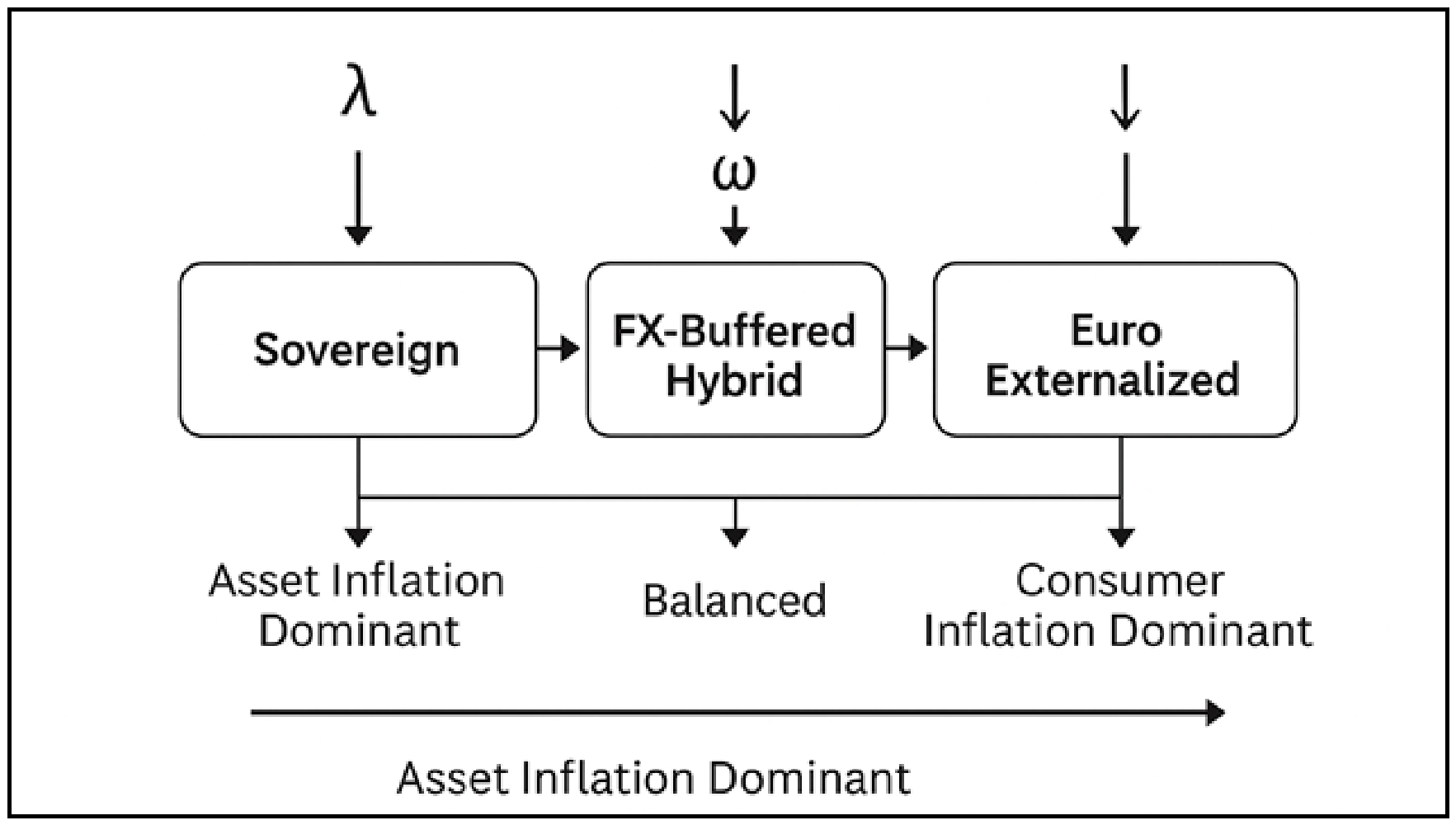
Sovereign Regime: High sterilization λsov ↑ and strong FX-buffer elasticity (ωsov). Asset–consumption spreads remain balanced or positive. Inflation is directed primarily into asset markets (housing, land), stabilizing consumer prices.
FX-Buffered Hybrid Regime: Partial decoupling from sovereignty as euroization deepens. Moderate λhyb and ωhyb; spreads begin to fluctuate but remain contained.
Euro Externalized Regime: Sterilization capacity collapses λeu → 0; FX buffers lose effectiveness (ωeu → 0); asset–consumption spreads inverts ()).
Interpretation: The transition path illustrates how diminishing functional sovereignty reshapes the structural composition of inflation, shifting from policy-anchored asset inflation toward externally driven consumer-price volatility. As ω (FX elasticity) and λ (sterilization control) decline, the system evolves from a regime of policy-determined nominal stability to one of externally constrained inflation transmission, culminating in the empirically observed structural inversion of asset–consumption spreads.
Appendix B. Supplementary Empirical Results: Panel ARDL Estimation
Appendix B.1. Panel Unit Root and Stationarity Tests
Table A1.
Panel unit root and stationarity tests.
Interpretation. All series are either I(0) or at most I(1), with none integrated of order I(2). This satisfies the central pre-condition of the ARDL bounds-testing framework (Pesaran et al., 2001), which admits a mix of I(0) and I(1) regressors but breaks down in the presence of I(2) variables. The CIPS statistics, which are robust to cross-sectional dependence, confirm this ordering for the series on which they could be estimated. For fiscal_balance_gdp, the CIPS statistic is not reported (“n.a.”), as the short time dimension left insufficient degrees of freedom for the cross-sectionally augmented regressions; its I(0) classification therefore rests on the IPS, LLC, and Fisher-ADF tests, which are mutually consistent.
Appendix B.2. Model Selection and Cointegration
Table A2.
ARDL Lag Selection Results.
Appendix B.3. Robustness—Per-Country Bounds Tests and the Decoupling Mechanism
To verify that the cointegration evidence is not an artefact of pooling, the conditional ARDL error-correction model is re-estimated country-by-country and subjected to the Pesaran et al. (2001) bounds F-test, for both the 10-year Maastricht yield and the short-term policy rate (int_rt). Because the time dimension is short (T = 23), asymptotic surface p-values are liberal; each statistic is therefore benchmarked against the more conservative Narayan (2005) small-sample critical values (Case III, k = 2).
Table A3.
Per-country bounds F-tests, both instruments (order/F).
We stress at the outset that non-rejection of the no-cointegration null is not itself direct proof of decoupling: with T = 23 the bounds test has limited power, so absence of a detected relationship is supported by, rather than established by, the test. The interpretation is therefore theory-led—and it is notable that the non-rejections cluster on the two polar monetary regimes. Bulgaria fails to reject in every specification and under both instruments: operating a currency board since 1997, it imports euro-area monetary conditions and severs the domestic fiscal-to-yield channel by construction, which is exactly what the regime predicts. The Czech Republic illustrates the instrument-dependence of the result: under the market-priced 10-year yield the channel is absent (both specifications non-reject), consistent with a freely floating koruna and an independent, inflation-targeting CNB that anchors yields to the domestic monetary stance rather than the fiscal position; under the policy rate, by contrast, cointegration reappears, since the short rate is the CNB’s own instrument and moves with the domestic cycle it targets.
The remaining economies localize the relationship rather than undermine it. Croatia—a de facto tightly managed ERM II peg prior to euro adoption in 2023—shows a refined, regime-specific pattern under both instruments: cointegration in the debt (stock) specification but not in the fiscal-balance (flow) specification, so the level of public debt remains anchored to the system while the flow of the balance does not transmit. Hungary displays the mirror image (flow-only), and Poland and Romania cointegrate under both indicators and both instruments. Where cointegration is present, it is carried by rate persistence and external foreign exchange inflows, not by the fiscal-stance variables, which remain statistically weak throughout. The convergence of the ARDL coefficients, the error-correction term, and the per-country bounds tests therefore supports a consistent reading: the fiscal → rate channel is weak, and where it is weakest, the institutional monetary regime predicts it should be.
Table A4.
Panel cointegration tests (Pedroni, 1999).
As a supplementary check, residual-based panel cointegration tests (Pedroni, 1999, 2004) were computed for all four specifications, combining each fiscal regressor (the fiscal balance and the government-debt ratio) with each interest-rate measure (the policy rate and the 10-year benchmark yield). The seven standardized statistics are distributed N(0,1) under the null of no cointegration, which is rejected for large negative values (−1.64 at the 5% level). As reported in Table A4, not a single statistic falls below this threshold in any of the four specifications: of twenty-eight statistics (seven per specification), zero reject the null. This uniformity is itself informative. Residual-based panel tests are known to have low power in short panels, and with only six cross-sectional units—further shortened to eighteen annual observations in the yield-based specifications, for which 10-year yields are available only from 2005—their failure to reject is unsurprising and carries little evidential weight. Primary cointegration inference therefore rests on the per-country bounds tests and on the error-correction term, which is correctly signed and strongly significant (−0.40, t = −3.68), indicating adjustment toward the long-run relationship. The Pedroni results are reported for completeness only; no inference rests upon them.
Appendix C. Cross Model Validation
Appendix C.1. Pre-Treatment Fit Across the Three Estimations
Table A5.
Pre-treatment fit across three estimators.
Gsynth is not treated as a co-equal effect estimator, and its diagnostics must be read with one distinction in mind: the cross-validated latent-factor count r* is a dimensionality parameter of the donor common component, not a goodness-of-fit statistic. To discipline this parameter, we report every Gsynth spread under leave-one-out cross-validation over r ∈ {0,…,5} on the full eleven-country donor pool, estimating all forty-nine reconciled spreads across three pre-treatment windows (2009, 2010, 2011). We make no claim that any particular r* validates the pre-period fit; the two can and do diverge, and the clearest illustration is internal to the furnishings result discussed below.
On the admissibility gate, the Gsynth evidence separates into three groups. The first is the set of fit-validated significant durable spreads. Two durable-versus-services contrasts are simultaneously significant and fit-admissible. COMPUT—HOTEL passes cleanly in both estimable windows (2010: ATT = −4.82, 90% CI [−8.59, −1.06], p = 0.035, R2 = 0.88, nRMSE = 0.34, r* = 5; 2011: ATT = −7.15, 90% CI [−11.29, −3.02], p = 0.004, R2 = 0.98, nRMSE = 0.14, r* = 5), and its factor selection is robust—widening the search range to r ∈ {0,…,8} leaves r* = 5 unchanged, confirming that the selected dimensionality is not an artefact of a binding search ceiling. FURN—FOOD is likewise significant and fit-admissible in both windows (2010: ATT = −3.99, 90% CI [−6.46, −1.51], R2 = 0.72, nRMSE = 0.51, r* = 4; 2011: ATT = −4.35, 90% CI [−7.24, −1.46], R2 = 0.72, r* = 4), with the durable-goods effect robust at p < 0.001. We attach one caveat to its fit statistic, not its effect: when the factor search is widened to r ∈ {0,…,8}, FURN—FOOD selects r* = 7 and its pre-period R2 rises to 0.91, so the reported R2 = 0.72 is itself a function of the factor ceiling and should be read as an admissibility figure under the canonical r ≤ 5 rule rather than as a fixed fit value. The point estimate and its significance are stable across both ranges; it is only the fit statistic that moves with r. This is precisely why r* and goodness-of-fit must be read as distinct quantities.
The second group is significance without fit. FURN—HOTEL is significant in every window (ATT ranging from −3.88 to −4.86, all 90% CIs excluding zero) yet carries a negative pre-period pseudo-R2 throughout (−0.35 in 2009, deteriorating to −0.93 in 2011) and nRMSE above unity in every case, so its synthetic counterfactual reproduces pre-treatment Croatia less well than a flat mean. It fails the admissibility gate outright and no inference rests on it; it is retained only as the textbook instance that significance and fit need not coincide. The global pre-period minimum across all reconciled spreads falls on this contrast (FURN—HOTEL 2011, R2 = −0.93).
The third group concerns the two fit-passing significant positive spreads that appear in the full panel (hpi_new—FOOD and hpi_total—FOOD, both 2009, ATT ≈ +10, R2 ≈ 0.67–0.71). These involve house-price indices rather than consumer-price components and therefore lie outside the durable-goods inflation question entirely; we report them for completeness and draw no substantive inference from them.
Two conclusions follow, and they refine rather than overturn this paper’s reading of Gsynth. First, under a disciplined cross-validated donor-based counterfactual, Gsynth does provide fit-admissible significant corroboration for the durable-goods signal—in two independent durable-versus-services contrasts (COMPUT—HOTEL and FURN—FOOD), both negative, both significant, both clearing the admissibility gate. This is stronger than a mere structural plausibility check and we say so. Second, there is no aggregate sign-asymmetry to speak of: across the forty-two consumption-component spreads, the share of negative point estimates is 0.48, 0.45 and 0.50 in the three windows, and a one-sided binomial test against p = 0.5 is non-significant in every window and every anchor class (pbinom between 0.56 and 0.94). The Gsynth signal is therefore not a diffuse downward tilt across the consumption basket; it is concentrated in the specific fit-passing durable contrasts. Accordingly, we do not characterize the aggregate as sign-asymmetric or as “sensitive” to the counterfactual—the aggregate is approximately symmetric, and the economically meaningful result is the localized, fit-validated durable effect. The cross-model robustness claim rests primarily on the two self-extrapolating estimators that clear the strict (R2 > 0.90) standard—the BSTS Hybrid, corroborated by Causal Impact—with Gsynth entering as a donor-based structural check that, under cross-validation, independently confirms the durable-goods direction in its two admissible spreads.
Appendix C.2. Cross-Model Covariate Stability Matrix
We fix k = 2 a priori on theoretical grounds (as stated in the code comments). We note that the Kaiser criterion (λ > 1) would in fact suggest three components in two of the three windows (2009: λ3 = 1.20; 2010: λ3 = 1.10), while the 2011 window (λ3 = 0.96) supports two. We deliberately retain two components despite this, for two reasons: (a) With only 12–14 pre-treatment observations, the BSTS model with a spike-and-slab prior tolerates only a low ratio of candidate regressors to observations; adding a third component alongside the donor columns dilutes the posterior inclusion probabilities and destabilizes the counterfactual estimate. (b) Two components already explain 75–81% of the variance of the six confounders across all windows (Appendix C Table A6), so the marginal information gain from a third component does not justify the loss of parsimony. The choice of k = 2 therefore prioritizes estimation stability over maximal variance coverage, consistent with the small pre-treatment sample. Moreover, keeping the BSTS control set minimal preserves comparability across methods: the two robustness checks (Causal Impact and Gsynth) operate without confounder controls; Gsynth drops them as collinear with the time effects, and Causal Impact relies solely on the donor series—so a parsimonious two-component specification keeps the BSTS Hybrid as close as possible to the control-free designs against which it is benchmarked.
Table A6.
Cross-model covariate stability matrix.
Two principal components explain between 75% and 81% of the variance of the six confounders across all three windows.
Table A7.
Loadings of PC1 and PC2.
Interpretation of the Principal Components
PC1—Real-Fiscal Strength (Cyclical Dimension): PC1 is remarkably stable across all three windows. It loads positively on fiscal balance (+0.47 to +0.52) and GDP per capita (+0.49 to +0.51), and negatively on unemployment (−0.30 to −0.48) and interest rates (−0.44 to −0.48). It captures periods of a healthy, expanding economy with favorable financial conditions. The signs remain virtually unchanged across windows, indicating a robust and economically interpretable component.
PC2—Debt and External-Monetary Dimension: PC2 is dominated by public debt, which loads strongly and consistently (+0.56 to +0.63) across all windows, together with negative loadings on interest rates (−0.35 to −0.45). In the 2010 and 2011 windows, fx_after_steril also loads strongly and negatively (−0.66 and −0.62, respectively). This component captures an MMT-relevant regime characterized by high public debt, suppressed interest rates, and sterilized foreign exchange conditions—precisely the dimension associated with a loss of monetary autonomy.
One caveat should be explicitly acknowledged. The positions of unemployment and fx_after_steril migrate across components over the windows (for example, unemployment loads positively on PC2 in 2009 (+0.545) but is essentially absent from PC2 in 2010–2011). While PC1 is rotationally stable, PC2 is less stable in its secondary loadings. This is expected given the small sample size of only 12–14 observations and should be reported rather than smoothed over.
Appendix D. Placebo and Robustness Tests
Table A8.
Prior sensitivity analysis.
Figure A2.
Prior-sensitivity heatmap. Note: * = significant at 90% (posterior credible interval excludes 0). Dashed border = ESS < 269 (non-converged, excluded).
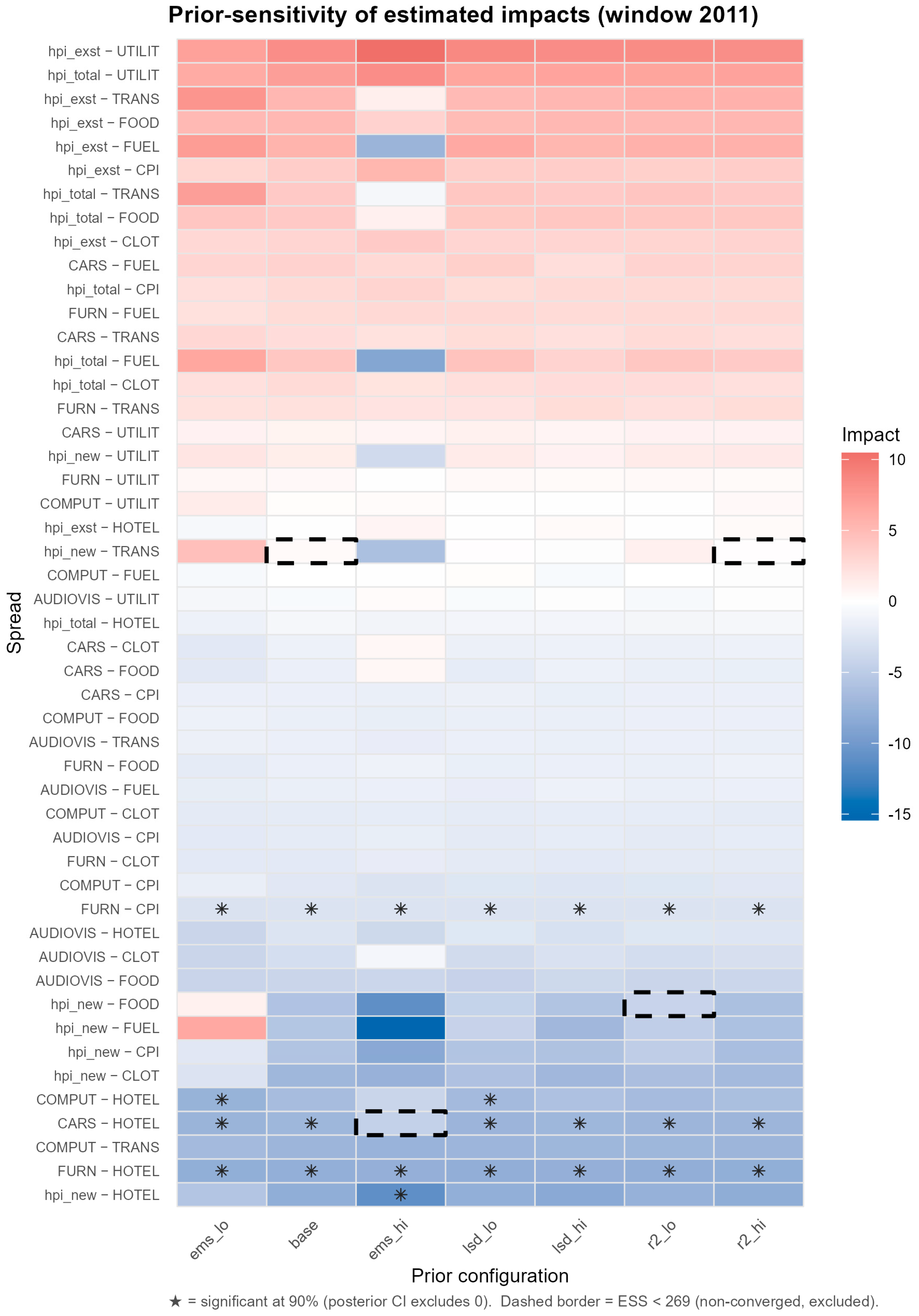
Appendix E
Convergence Diagnostics—Bayesian Estimation Diagnostics
Figure A3.
Geweke z-statistic against effective sample size. Note: Geweke z-statistic against effective sample size for all 147 treatment-effect posteriors (log-scaled x-axis). The shaded band marks the non-rejection region (|z| < 1.96). Red triangles denote the 10 posteriors for which the Geweke test rejects stationarity; all lie to the right of ESS = 400, well above the retention threshold ESS = 269. Source: authors’ calculations.
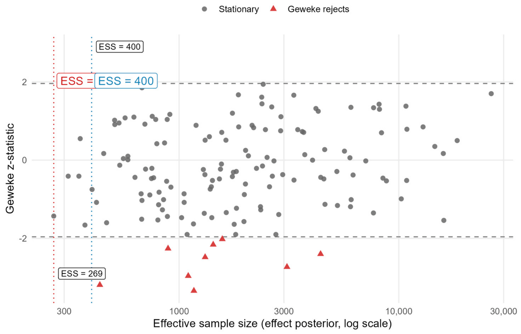
Table A9.
Effective sample size and Geweke diagnostics.
Appendix F. Auxiliary BSTS Re-Estimation on a Non-Euro CEE Donor Pool
Appendix F.1. Purpose and Scope
The baseline BSTS specification is re-estimated using an alternative donor pool consisting exclusively of non-euro Central and Eastern European economies (Poland, Hungary, the Czech Republic, and Romania). The estimation procedure is otherwise identical to the baseline specification, including the asset and consumption series, pre-treatment windows (2009, 2010, and 2011), priors, and posterior significance criteria. This appendix reports the complete results of the auxiliary robustness analysis.
Appendix F.2. Results
Table A10.
Pooled sign test by pre-treatment start window (exact binomial test): full output.
A comparison with the baseline indicates a weaker inversion pattern under the non-euro donor pool. The negative share remains close to one-half across most cells, and statistical significance is substantially reduced after adjustment for multiple testing.
Table A11.
Sign test of the Spread () by post-year, pre-treatment window, and anchor type (auxiliary non-euro donor pool).
Appendix F.3. Interpretation
The auxiliary specification produces a weaker and more balanced inversion pattern than the baseline specification. The difference is concentrated in the housing (HPI) anchor, whereas the durables-versus-consumption and headline-CPI anchors continue to display predominantly negative effects. In the later-year housing cells, the pattern is not merely attenuated but locally reversed: under the consumption anchor, the 2025 negative share falls to 0.405 with a positive median spread. These findings indicate that donor-pool composition primarily affects the housing-price channel—in both magnitude and, in places, direction—while the remaining inflation channels remain comparatively stable.
The auxiliary specification nevertheless yields a technically valid, though substantively different, estimate. The objective of the baseline model is to identify the marginal effect of euro adoption while holding Croatia’s broader macro-financial environment as constant as possible. This requires a donor pool that resembles Croatia not only in observable characteristics but also in its monetary transmission mechanism.
The non-euro CEE economies differ simultaneously from Croatia along several dimensions that were highly active during 2021–2023, including autonomous monetary policy, floating exchange rates, and substantially stronger exchange-rate pass-through into domestic inflation. During the inflation peak, Hungary (approximately 25%), Poland (approximately 18%), the Czech Republic (approximately 18%), and Romania (approximately 16%) all experienced substantially higher inflation than Croatia (approximately 13.5% in November 2022). These differences largely reflect exchange-rate movements and country-specific monetary policy rather than euro adoption itself. Consequently, interpolation bias may influence the estimated treatment effect when these countries are used as synthetic controls.
Appendix F.4. Pre-Treatment Divergence
An important diagnostic concerns the timing of divergence. If the observed inflation differential between Croatia and the non-euro donor pool were generated by euro adoption, the divergence should emerge only after January 2023. Instead, the differential is already clearly visible during 2021–2022, well before treatment. This pre-treatment divergence contaminates the counterfactual trajectory and weakens causal attribution.
Accordingly, the non-euro donor pool captures an existing structural difference between Croatia and the floating CEE economies rather than isolating the marginal effect of euro adoption. This is the principal reason why the specification is reported as an auxiliary robustness exercise rather than as the baseline model.
Figure A4.
Divergence of real estate and consumer inflation, Croatia. Source: authors’ calculations. Note: The 2000–2022 window refers to the ARDL specification testing the decoupling axiom on the covered macro variables (excluding HPI). Figure A4 reports the BSTS estimation sample, for which the Croatian HPI series is first available in 2009 (hence the 2009–2025 span). Dotted line = onset of divergence (2016); dashed line/shaded area = post-euro (2023–). Panel (A) plots the two-inflation series; Panel (B) plots the raw level spread (HPI—mean consumption), not the BSTS causal impact. Series are distinguished by marker shape and line type rather than color to preserve legibility in grayscale print.
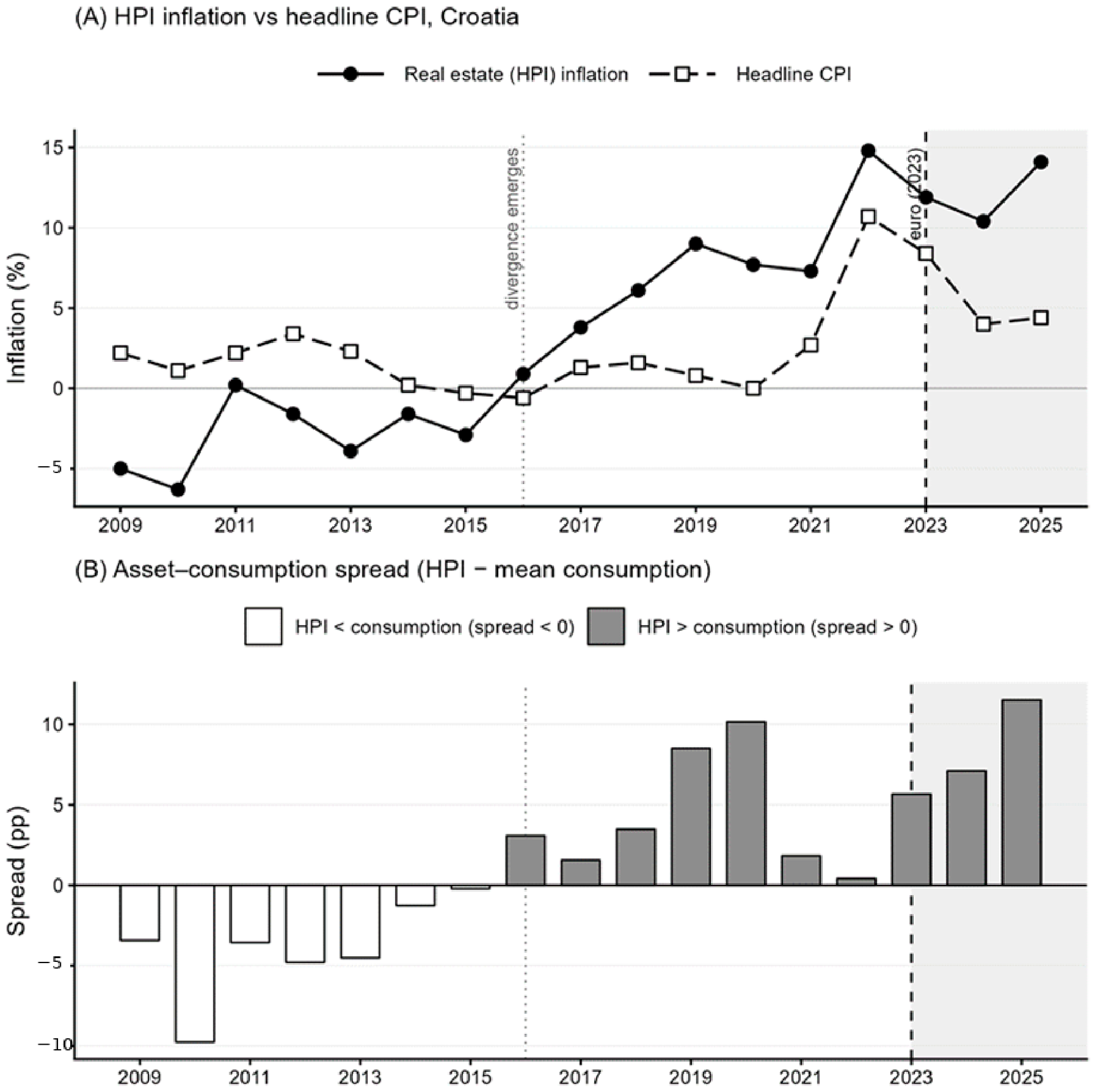
References
- Aoki, K. (2001). Optimal monetary policy responses to relative-price changes. Journal of Monetary Economics, 48(1), 55–80. [Google Scholar] [CrossRef] [Scilit]
- Bańbura, M., & Modugno, M. (2014). Maximum likelihood estimation of factor models on datasets with arbitrary pattern of missing data. Journal of Applied Econometrics, 29(1), 133–160. [Google Scholar] [CrossRef] [Scilit]
- Bell, S. (2000). The role of the state and the hierarchy of money. Cambridge Journal of Economics, 25(2), 149–163. [Google Scholar] [CrossRef] [Scilit]
- Blanchard, O., & Galí, J. (2007). Real wage rigidities and the New Keynesian model. Journal of Money, Credit and Banking, 39(s1), 35–65. [Google Scholar] [CrossRef] [Scilit]
- Blanchard, O., & Pisani-Ferry, J. (2022). Fiscal and monetary coordination in the post-pandemic EU. Fiscal support and monetary vigilance: Economic policy implications of the Russia Ukraine war for the European Union policy briefs PB22-5, Peterson institute for international economics working paper 23-1. Peterson Institute for International Economics. Available online: https://www.piie.com/sites/default/files/documents/pb22-5.pdf (accessed on 27 October 2026).
- Blyth, M. (2013). Austerity: The history of a dangerous idea. Oxford University Press. [Google Scholar]
- Borio, C., Disyatat, P., & Rungcharoenkitkuli, P. (2019). What anchors for the natural rate of interest? (BIS Working Papers 777). Bank for International Settlements. Available online: https://ideas.repec.org/p/bis/biswps/777.html (accessed on 27 October 2026).
- Brodersen, K. H., Gallusser, F., Koehler, J., Remy, N., & Scott, S. L. (2015). Inferring causal impact using Bayesian structural time-series models. Annals of Applied Statistics, 9(1), 247–274. [Google Scholar] [CrossRef] [Scilit]
- Cecchetti, S., Genberg, H., Lipsky, J., & Wadhwani, S. (2000). Asset prices and central bank policy (Geneva Reports on the World Economy, 2). International Center for Monetary and Banking Studies & Centre for Economic Policy Research. Available online: https://www.researchgate.net/publication/243663697_Asset_Prices_and_Central_Bank_Policy (accessed on 27 October 2026).
- Cesaratto, S. (2015). Balance of payments or monetary sovereignty? In search of the EMU’s original sin. International Journal of Political Economy, 44(2), 142–156. [Google Scholar] [CrossRef] [Scilit]
- Clarida, R., Gali, J., & Gertler, M. (1999). The science of monetary policy: A new Keynesian perspective. Journal of Economic Literature, 37(4), 1661–1707. [Google Scholar] [CrossRef] [Scilit]
- Croatian Bureau of Statistics. (2022). Annual report on wages and inflation. Croatian Bureau of Statistics. Available online: https://podaci.dzs.hr/en/statistics/labour-market/wages/ (accessed on 18 November 2025).
- Croatian Bureau of Statistics. (2024). Persons at risk of poverty or social exclusion. Croatian Bureau of Statistics. Available online: https://podaci.dzs.hr/2025/en/97252 (accessed on 19 November 2025).
- De Grauwe, P. (2020). Economics of monetary union. Oxford University Press. Available online: https://global.oup.com/ukhe/product/economics-of-monetary-union-9780198986096?cc=hr&lang=en& (accessed on 27 October 2026).
- De Hoyos, R. E., & Sarafidis, V. (2006). Testing for cross-sectional dependence in panel data. Stata Journal, 6(4), 482–496. [Google Scholar] [CrossRef] [Scilit]
- Driscoll, J. C., & Kraay, A. C. (1998). Consistent covariance matrix estimation with spatially dependent panel data. The Review of Economics and Statistics, 80(4), 549–560. [Google Scholar] [CrossRef] [Scilit]
- ECB (European Central Bank). (2022). Macroprudential oversight frameworks in the Eurozone. European Central Bank. Available online: https://finance.ec.europa.eu/financial-markets/financial-markets/macroprudential-policy/macroprudential-framework-banks_en (accessed on 4 July 2026).
- European Commission. (2023). AMECO database: Annual macroeconomic indicators. European Commission. Available online: https://economy-finance.ec.europa.eu/economic-research-and-databases/economic-databases/ameco-database_en (accessed on 21 November 2025).
- Farhi, E., & Werning, I. (2019). Monetary policy, bounded rationality, and incomplete markets. American Economic Review, 109(11), 3887–3928. [Google Scholar] [CrossRef] [Scilit]
- Fitoussi, J.-P., & Saraceno, F. (2010). Europe: How deep is a crisis? Policy responses and structural factors behind diverging performances. Journal of Globalization and Development, 1(1), 17. [Google Scholar] [CrossRef] [Scilit]
- Gabor, D. (2021). The wall street consensus: Financialization and the state in the post-COVID global economy. Development and Change, 52(3), 429–459. [Google Scholar] [CrossRef] [Scilit]
- Galí, J., & Monacelli, T. (2005). Monetary policy and exchange rate volatility in a small open economy. Review of Economic Studies, 72(3), 707–734. [Google Scholar] [CrossRef] [Scilit]
- Gelman, A., Carlin, J., Stern, H., Rubin, D., Dunson, D., & Vehtari, A. (2013). Bayesian data analysis (3rd ed.). CRC Press. Available online: https://sites.stat.columbia.edu/gelman/book/BDA3.pdf (accessed on 27 October 2026).
- Gibson, H. D., Palivos, T., & Tavlas, G. S. (2014). The crisis in the euro area: An analytic overview. Journal of Macroeconomics, 39, 233–239. [Google Scholar] [CrossRef] [Scilit]
- Goodhart, C., & Hofmann, B. (2008). House prices, money, credit, and the macroeconomy. Oxford Review of Economic Policy, 24(1), 180–205. [Google Scholar] [CrossRef] [Scilit]
- Goodhart, C., & Pradhan, M. (2020). The great demographic reversal: Ageing societies, waning inequality, and an inflation revival. Business Economics, 56, 113. [Google Scholar] [CrossRef] [Scilit]
- Hoechle, D. (2007). Robust standard errors for panel regressions with cross-sectional dependence. Stata Journal, 7(3), 281–312. [Google Scholar] [CrossRef] [Scilit]
- Honohan, P., & Lane, P. R. (2003). Divergent inflation rates in EMU. Economic Policy, 18(37), 357–394. [Google Scholar] [CrossRef] [Scilit]
- Im, K. S., Pesaran, M. H., & Shin, Y. (2003). Testing for unit roots in heterogeneous panels. Journal of Econometrics, 115(1), 56–69. [Google Scholar] [CrossRef] [Scilit]
- Kao, C. (1999). Spurious regression and residual-based tests for cointegration in panel data. Journal of Econometrics, 90(1), 1–44. [Google Scholar] [CrossRef] [Scilit]
- Kelton, S. (2020). The deficit myth: Modern monetary theory and the birth of the people’s economy. In Public affairs book (p. 336). Hachette Book Group. [Google Scholar]
- Lane, P. R. (2023). Inflation dynamics in the euro area: A reassessment. Dinner speech by Mr Philip R Lane, member of the executive board of the European Central Bank, at the money marketeers of New York university, New York City, 21 September 2023. Available online: https://www.bis.org/review/r230922d.htm (accessed on 27 October 2026).
- Levin, A., Lin, C. F., & Chu, C. S. J. (2002). Unit root tests in panel data: Asymptotic and finite-sample properties. Journal of Econometrics, 108(1), 1–24. [Google Scholar] [CrossRef] [Scilit]
- Marinov, M. (2021). pco: Panel cointegration estimation in R. Comprehensive R Archive Network. [Google Scholar]
- Mitchell, W., & Fazi, T. (2017). Reclaiming the state: A progressive vision of sovereignty for a post-neoliberal world (p. 320). Pluto Press. [Google Scholar]
- Narayan, P. K. (2005). The saving and investment nexus for China: Evidence from cointegration tests. Applied Economics, 37(17), 1979–1990. [Google Scholar] [CrossRef] [Scilit]
- Nenovsky, N. (2020). The theory of the emission economy Bolshevik roots of “modern monetary theory” (MPRA Paper No. 113048 Hal Open Science). University Library of Munich. Available online: https://u-picardie.hal.science/hal-04084551v1 (accessed on 27 October 2026).
- Palley, T. I. (2013). Financialization: The economics of finance capital domination (p. 231). Palgrave Macmillan. [Google Scholar]
- Pedroni, P. (1999). Critical values for cointegration tests in heterogeneous panels with multiple regressors. Oxford Bulletin of Economics and Statistics, 61, 653–670. [Google Scholar] [CrossRef]
- Pedroni, P. (2004). Panel cointegration: Asymptotic and finite sample properties. Econometric Theory, 20(3), 597–625. [Google Scholar] [CrossRef] [Scilit]
- Pesaran, M. H. (2007). A simple panel unit root test in the presence of cross-section dependence. Journal of Applied Econometrics, 22(2), 265–312. [Google Scholar] [CrossRef] [Scilit]
- Pesaran, M. H., Shin, Y., & Smith, R. J. (2001). Bounds testing approaches to the analysis of level relationships. Journal of Applied Econometrics, 16(3), 289–326. [Google Scholar] [CrossRef] [Scilit]
- Piketty, T. (2014). Capital in the twenty-first century. Harvard University Press. [Google Scholar]
- Reinhart, C., & Reinhart, M. (2011). Diminished expectations, double dips, and external shocks: The decade after the fall (NBER Working Papers). National Bureau of Economic Research. Available online: https://www.nber.org/ (accessed on 27 October 2026).
- Scott, S. L., & Varian, H. R. (2014). Predicting the present with Bayesian structural time series. International Journal of Mathematical Modelling and Numerical Optimisation, 5(1–2), 4–23. [Google Scholar] [CrossRef] [Scilit]
- Stiglitz, J. E. (2016). The euro: How a common currency threatens the future of Europe (p. 512). W.W. Norton & Company. Available online: https://wwnorton.com/books/9780393354102 (accessed on 27 October 2026).
- Stockhammer, E. (2015). Rising inequality as a cause of the present crisis. Cambridge Journal of Economics, 39(3), 935–958. [Google Scholar] [CrossRef] [Scilit]
- Tymoigne, É., & Wray, L. R. (2013). Modern monetary theory 101: A reply to critics (Levy Economics Institute Working Paper No. 778). Levy Economics Institute of Bard College. Available online: https://www.levyinstitute.org/pubs/wp_778.pdf (accessed on 27 October 2026).
- Vehtari, A., Gelman, A., Simpson, D., Carpenter, B., & Bürkner, P. C. (2021). Rank-normalization, folding, and localization: An improved R-hat for assessing convergence of MCMC. Bayesian Analysis, 16(2), 667–718. [Google Scholar] [CrossRef] [Scilit]
- Westerlund, J. (2007). Testing for error correction in panel data. Oxford Bulletin of Economics and Statistics, 69(6), 709–748. [Google Scholar] [CrossRef] [Scilit]
- World Bank. (2000–2025). World development indicators (WDI). World Bank. Available online: https://databank.worldbank.org/source/world-development-indicators (accessed on 27 October 2026).
- Wray, L. R. (2012). Modern monetary theory: A primer on macroeconomics for sovereign monetary systems (p. 302). Palgrave Macmillan. [Google Scholar] [CrossRef] [Scilit]
- Wray, L. R. (2015). Why Minsky matters: An introduction to the work of a maverick economist (p. 273). Princeton University Press. [Google Scholar]
- Wyplosz, C. (2014). The Eurozone crisis: A near-perfect case of mismanagement. Economia Marche Journal of Applied Economics, XXXIII(1), 1–13. [Google Scholar]
- Xu, Y. (2017). Generalized synthetic control method: Causal inference with interactive fixed effects models. Political Analysis, 25(1), 57–76. [Google Scholar] [CrossRef] [Scilit]
- Zimmermann, C. D. (2014). A contemporary concept of monetary sovereignty. Oxford University Press. [Google Scholar]
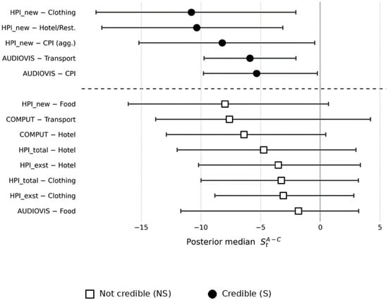
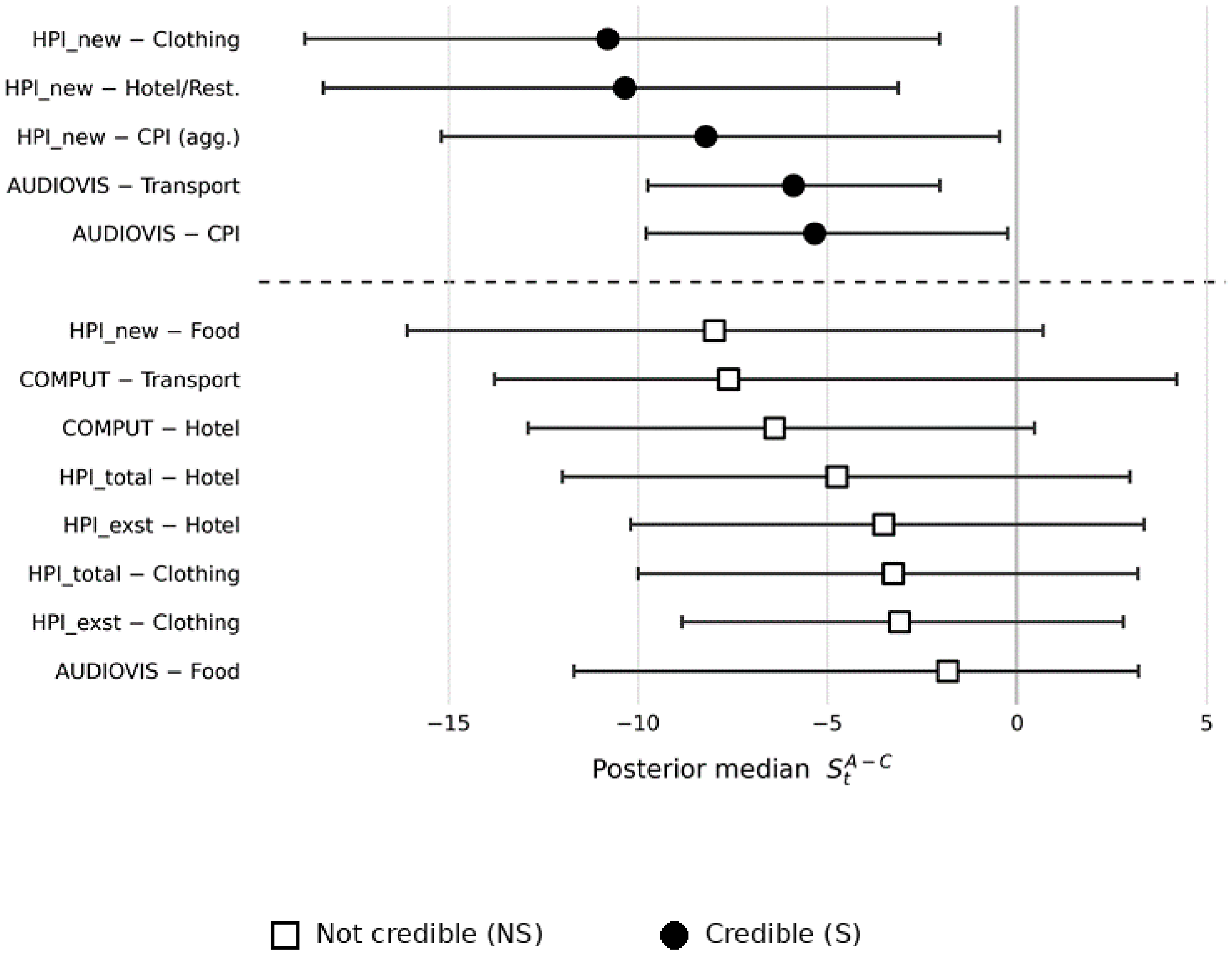
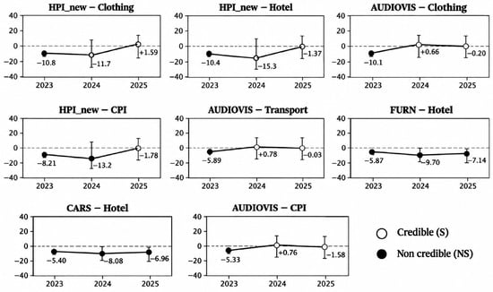
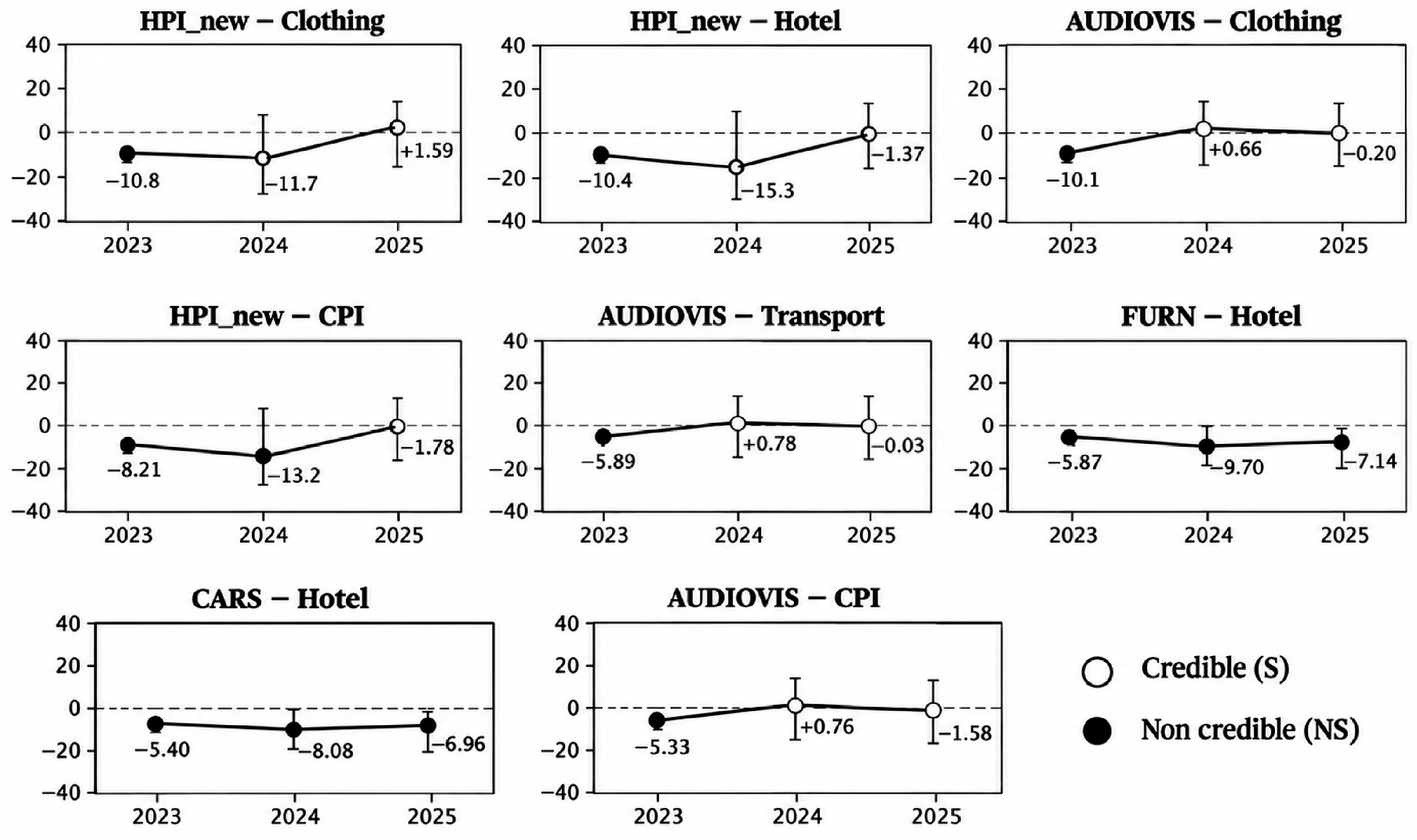
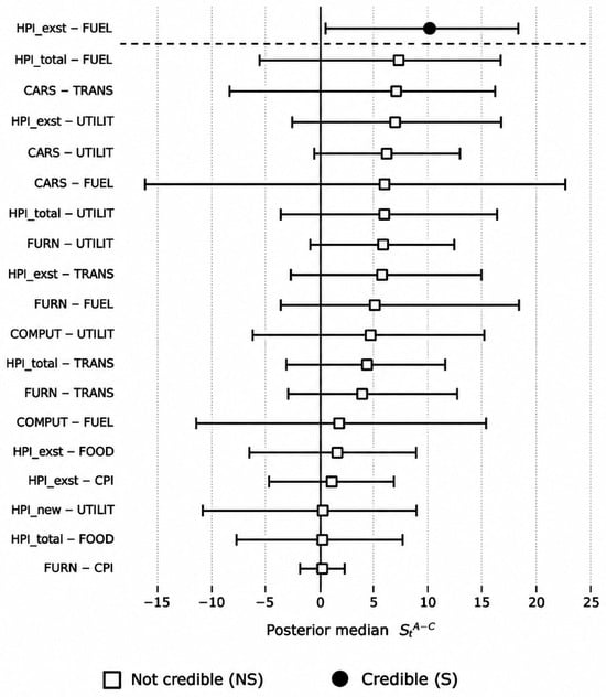
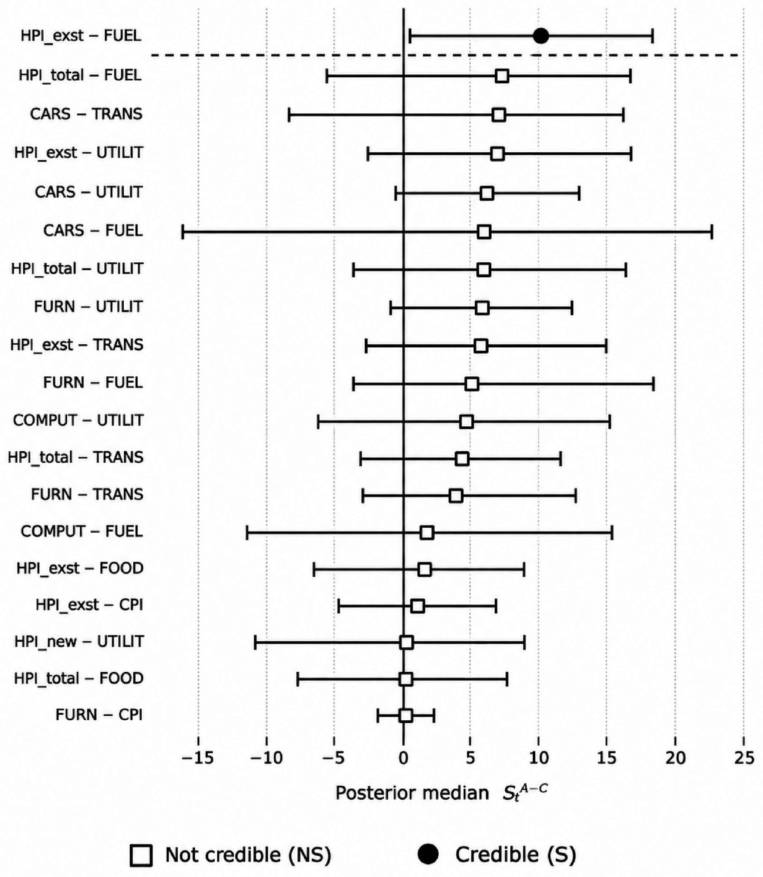
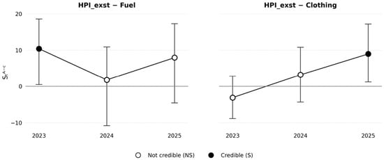
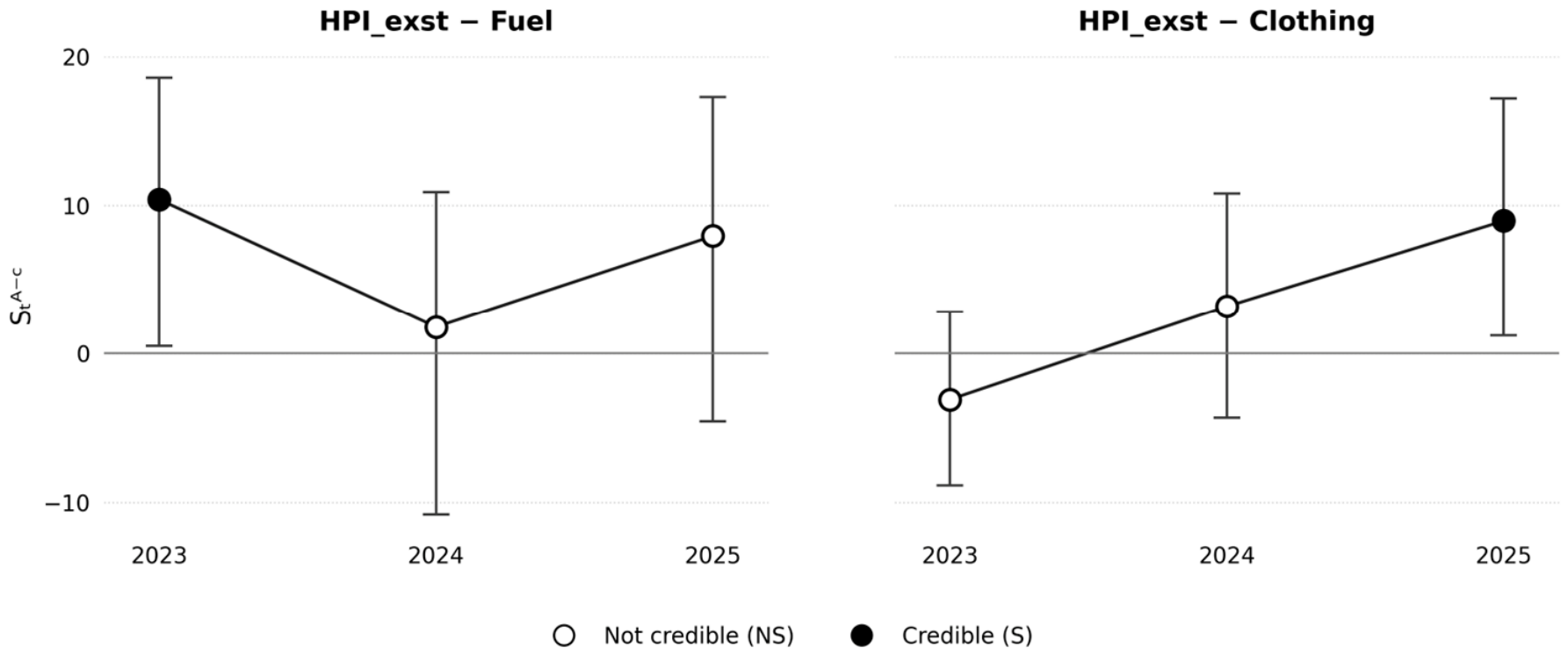
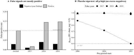
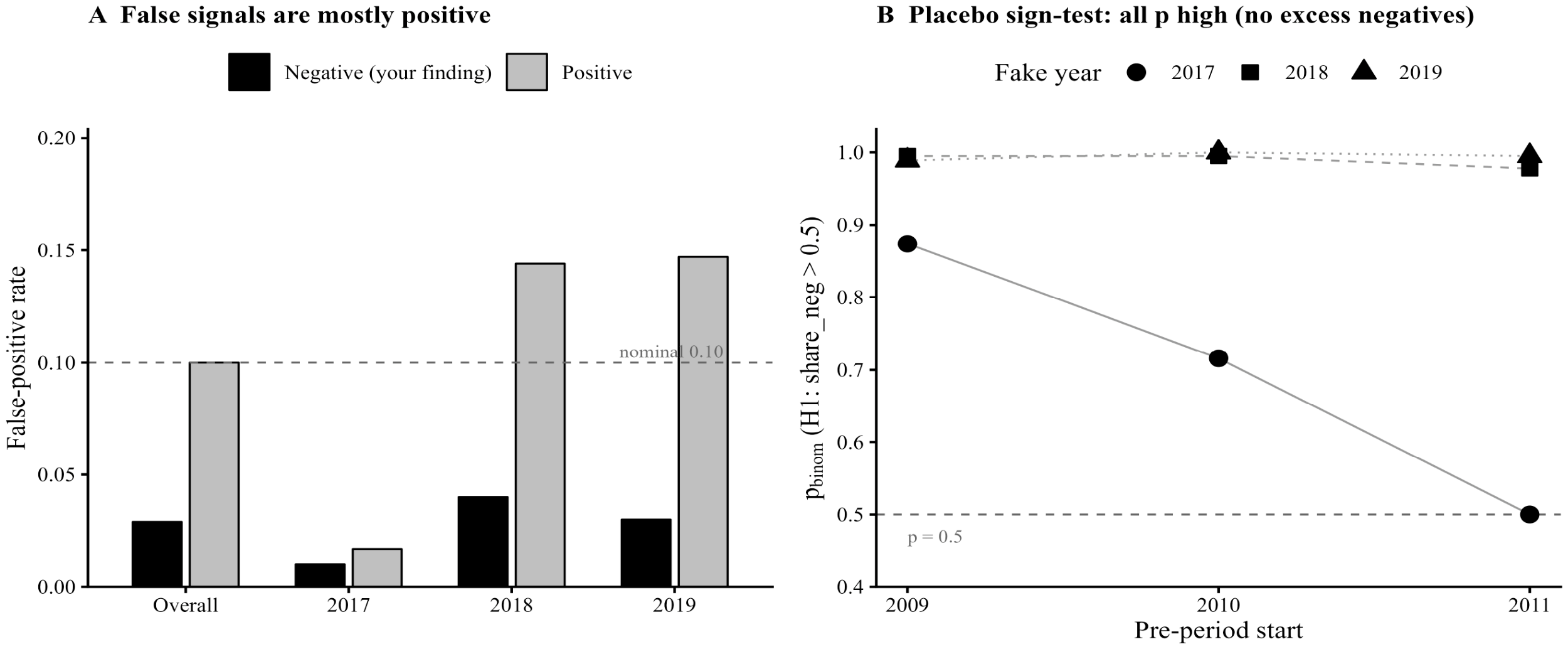

Disclaimer/Publisher’s Note: The statements, opinions and data contained in all publications are solely those of the individual author(s) and contributor(s) and not of MDPI and/or the editor(s). MDPI and/or the editor(s) disclaim responsibility for any injury to people or property resulting from any ideas, methods, instructions or products referred to in the content. |
© 2026 by the authors. Licensee MDPI, Basel, Switzerland. This article is an open access article distributed under the terms and conditions of the Creative Commons Attribution (CC BY) license.