


Abstract
We investigate whether joint revenue–expenditure dynamics and additional macroeconomic information improve one-year-ahead fiscal-balance forecasts. A revised Eurostat panel of 27 present-day EU countries over 2009–2025 is evaluated at 324 country-year targets in 2014–2025, with an extended 1995–2025 panel used to assess training-history sensitivity. Joint pooled VAR(1) yields a balance MAE of 1.626 percentage points of GDP, compared with 1.725 for persistence, 1.727 for separate component autoregressions, and 1.619 for direct balance AR(1). Its gain is concentrated in 2020–2022, and the two-year block-bootstrap interval for its gain includes zero. Component scores show a small expenditure improvement but no revenue improvement over persistence. Training-window ridge selection improves the penalised comparator, while lagged GDP growth, GDP-deflator growth and interest expenditure do not improve matched-sample accuracy. A separate archived-autumn experiment uses information recorded at each forecast origin and spring-after-target outcomes. Adding the European Commission’s contemporaneously available GDP and price outlook reduces direct-model MAE from 1.875 to 1.769; the Commission’s own balance forecast remains more accurate at 1.637. The contribution is a reproducible separation of cross-dynamics, information timing and regime sensitivity, rather than a claim of universal joint-model superiority.
1. Introduction
A useful fiscal forecast must distinguish an accounting requirement from an empirical advantage. Revenue and expenditure projections can be combined into a balance that satisfies the budget identity, but consistency alone does not establish accuracy. Errors in the two components can reinforce or offset one another. A direct forecast of the balance may therefore be competitive even when the individual fiscal series are strongly persistent and interdependent.
This distinction matters for fiscal planning in Europe. The sovereign-debt crisis, pandemic and energy-price disturbances altered revenue bases, spending needs and GDP denominators. Institutions and policy announcements also influence budget outcomes. The statistical problem is consequently not whether an elaborate model fits historical observations, but whether additional dynamics or information reduce error at genuinely withheld forecast targets. Forecast evaluation must also identify whether historical data were revised after the decision date (Tashman, 2000; Beetsma et al., 2009; Frankel, 2011).
Existing research addresses complementary parts of this problem. Carriero et al. (2015) examine richer multivariate fiscal forecasting; institutional evaluations assess official macroeconomic and fiscal projections; and research on forecast practices highlights timing and institutional differences. The gap addressed here is narrower: within a common country-panel exercise, how much comes from cross-series dynamics, how much from the information set, and how stable are the apparent improvements across target years? We do not claim to introduce a new forecasting estimator.
We answer three questions. RQ1: Do cross-series dynamics improve the accuracy of component and balance forecasts relative to separate autoregressions and direct balance forecasting? RQ2: Do additional lagged macroeconomic variables or contemporaneously available macroeconomic projections improve a matched direct or joint benchmark? RQ3: How sensitive are the comparative results to crisis years, training-history length, model tuning, and the treatment of data vintages?
The design has deliberately separate parts. The original revised-data backtest is retained so the cross-dynamic comparison remains transparent. A longer historical panel tests training sensitivity. Matched-sample macroeconomic specifications test richer predictors. Finally, an archived-information exercise evaluates direct forecasts and the Commission’s autumn benchmark using the same first-post-year spring outcome definition. We do not merge these exercises into one accuracy ranking because their information sets and outcome vintages differ.
The results support a qualified contribution. Joint VAR(1) beats separate component autoregressions on balance MAE but is almost matched by direct AR(1), and its aggregate advantage over persistence is crisis-dependent. Lagged macroeconomic variables do not help in the tested specifications. By contrast, the origin-specific macroeconomic outlook improves the archived direct model, although the Commission’s own fiscal projection remains better. These findings identify the limits of extrapolation and the importance of information timing.
2. Literature and Institutional Framework
2.1. Fiscal Forecasts and Institutional Information
Fiscal forecasts combine economic projections with assumptions about tax rules, expenditure commitments, and policy implementation. Beetsma et al. (2009) examine deviations between fiscal plans and outcomes in real time; Frankel (2011) analyses optimism in official budget projections. These studies motivate attention to the origin of a forecast and the information incorporated in it. A forecast incorporating announced measures is not informationally equivalent to an autoregression of past fiscal ratios.
Büttner and Kauder (2009) compare revenue-forecasting practices across selected OECD countries and associate differences in precision with forecast timing, tax structures and aspects of methods and institutions. Their cross-country evidence motivates a timing-aware benchmark; it does not establish that adding variables to any particular panel regression must improve prediction. The Commission’s study of uncertainty in revenue prediction likewise places the dispersion of forecast errors at the centre of fiscal assessment (European Commission, 2016).
The institutional benchmark used here is the European Commission’s autumn forecast for the following year. The European Fiscal Board Secretariat’s Forecast Tracker stores these projections and outcomes recorded in spring after the target year. This matches a practical surveillance convention while avoiding the assumption that today’s revised historical figures were available to past forecasters. The benchmark incorporates professional judgement and policy information that are absent from our small statistical models (European Fiscal Board Secretariat, 2026).
Budget institutions also clarify why coherent revenue and expenditure projections may be useful even when balance accuracy changes little. Pešić and Miljković (2020) discuss budget principles and the preparation, adoption, execution, and control stages. Ćurčić (2025) examines expenditure financing under budget constraints, including the pressures associated with extraordinary spending. These perspectives motivate presenting both fiscal components alongside their difference: an unchanged projected balance can conceal different revenue and expenditure paths, with different implications for budget preparation.
Milanović (2022) discusses internal controls and public-sector audit, providing context for the oversight of budget execution. Škrbić et al. (2023) examine planning and resource constraints with particular attention to defence financing, while Škrbić and Obrić (2024) discuss the budgetary and legal setting of defence expenditure. These sectoral and institutional accounts help explain why forecasts must be interpreted alongside spending responsibilities and implementation procedures. They are contextual illustrations, not evidence that the estimated relationships apply uniformly across EU countries. The present aggregate panel does not identify the effects of audit quality, budget rules or defence commitments. Their relevance is therefore to the intended use and limitations of the forecasts; model accuracy is assessed separately through the held-out comparisons below.
2.2. Joint Systems and Direct Forecasts
Carriero et al. (2015) study Bayesian vector autoregressions with larger information sets and changing parameters for fiscal aggregates in the United States and major European economies. They find that information breadth and time variation can help, with different implications for point and density forecasts. Their design differs materially from a pooled annual two-variable panel: a small VAR does not reproduce the information content or shrinkage structure of their larger systems. We therefore use that study to motivate an explicit information-set extension rather than treating it as evidence that the baseline model must dominate.
Direct and component-based forecasts answer related but distinct operational needs. Direct balance autoregression is economical when the deficit is the only target. Joint forecasts additionally provide the two components, but their balance accuracy depends on the covariance and bias of component errors. Separate component autoregressions are an essential intermediate benchmark because they preserve the accounting subtraction without estimating cross-series lags. Comparing all three reveals whether any benefit is attributable to cross-dynamics rather than merely to constructing a balance.
Long-run fiscal sustainability studies address a different estimand. Afonso and Coelho (2022), for example, discuss fiscal reactions and sustainability. Such evidence helps frame the policy relevance but does not validate the short-run predictive coefficients estimated here. We neither interpret a predictive lag as a causal policy response nor impose cointegration without testing the required assumptions.
2.3. Evaluation Across Vintages and Exceptional Years
Chabin et al. (2020) assess the accuracy of the European Commission’s macroeconomic forecasts, while Axioglou et al. (2025) extend the institutional evaluation to pandemic and energy-crisis conditions and examine GDP growth, inflation and the government balance. Their scope motivates separate evaluation of exceptional years rather than inference from one full-period average. Our contribution differs by isolating simple panel-model alternatives, component errors and the incremental role of an origin-specific macroeconomic outlook.
MAE, RMSE and signed bias capture different features of performance (Hyndman & Koehler, 2006). Expanding-origin evaluation respects the temporal order of estimation and scoring (Tashman, 2000), but it does not by itself remove revision-based information advantages. Broad forecasting reviews also emphasise benchmarking and the dependence of performance on the forecasting task (Petropoulos et al., 2022). We therefore report separate experiments and treat the new comparisons as reviewer-motivated extensions, not as a preregistered confirmatory exercise.
3. Data and Methods
3.1. Revised Fiscal Panel and Historical Extension
The primary panel is extracted from the supplied Eurostat AGFS workbook AGFS_Tables_2026-10-21_S13_only.xlsb. It contains annual general-government total revenue (TR) and expenditure (TE), each expressed as a percentage of GDP, for 27 present-day EU countries in 2009–2025: 459 country-year observations with no missing component values. The workbook filename date identifies the supplied file; its status as an official publication timestamp is not independently established. The supplementary package (Supplementary Materials) records checksums, extraction coordinates, and year-header checks. The reference statistical series is gov_10a_main (Eurostat, 2026).
The geographical panel is fixed to today’s 27 members. It is not the historical EU membership in every year: notably, Croatia joined during the period. Each country receives equal weight in the scores and descriptive means. These means are not the official GDP-weighted EU aggregate. The 2009 start preserves the original design spanning debt-crisis, pandemic and recovery conditions; it is not selected by maximising forecast performance.
To examine dependence on the short training history, the same workbook is extended back to 1995. The resulting 31-year panel has 837 country-years and complete TR and TE observations for all 27 countries. The extension changes the estimation history while keeping the 2014–2025 forecast targets unchanged. Earlier observations may embody retrospective harmonisation and structural breaks; more observations are not automatically more informative about the recent fiscal regime.
bi,t = ri,t − ei,t
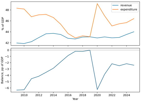
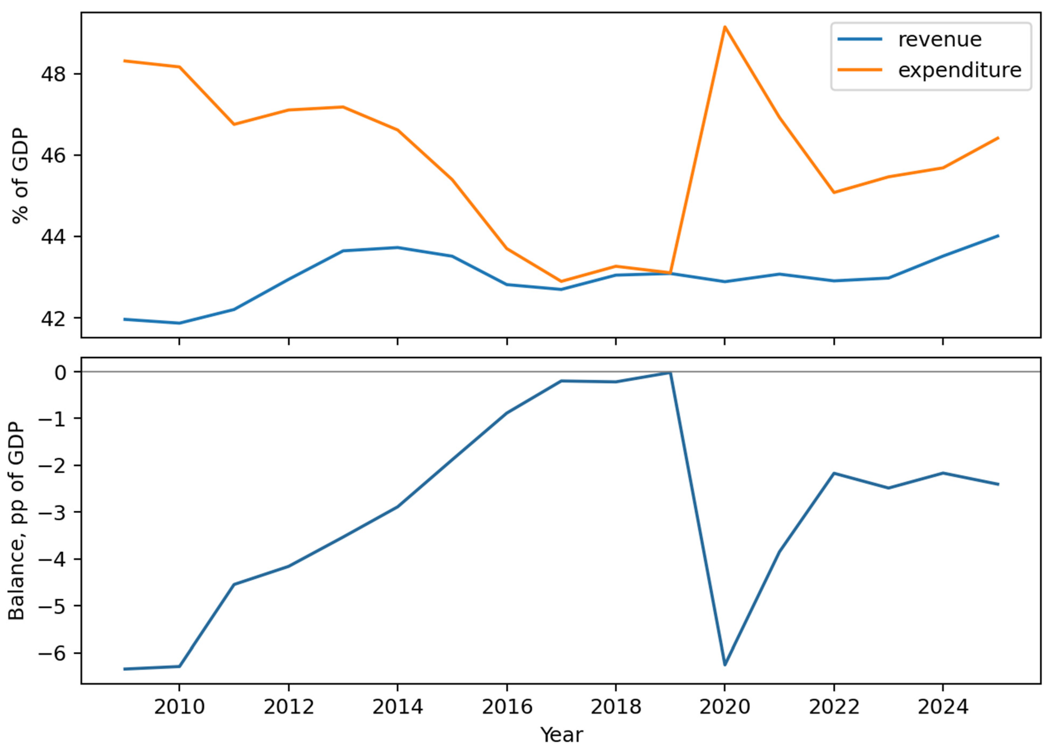
Here r and e denote revenue and expenditure shares, and b is net lending (+) or net borrowing (−), in percentage points of GDP. These are annual general-government accounting ratios, not nominal appropriations or cash-budget forecasts. Forecasting national-currency amounts would require additional GDP projections (European Central Bank, n.d.). Figure 1 shows the unweighted country means of revenue, expenditure and the balance.
Figure 1.
Unweighted country means for 27 present-day EU countries, 2009–2025. Revenue and expenditure are separated from the balance panel to preserve scale readability. Source: Authors’ calculations based on Eurostat AGFS data (Eurostat, 2026).
3.2. Joint and Direct Specifications
ri,t = αr + φrr ri,t−1 + φre ei,t−1 + ur,i,t
ei,t = αe + φer ri,t−1 + φee ei,t−1 + ue,i,t
The pooled VAR(1) estimates a common intercept and lag coefficients in each equation. Cross-series terms are φᵣe and φeᵣ; each equation also contains its own lag. Separate AR(1) equations omit the cross-series term but retain separate intercepts and own-lag slopes. Direct AR(1) instead regresses the balance on its own lag. Persistence uses the previous observation without coefficient estimation. All estimated rules are refitted at each forecast origin.
The induced joint balance is not algebraically identical to direct AR(1) without restrictions. Subtracting (3) from (2) produces an intercept difference and coefficients (φᵣᵣ − φeᵣ) and (φᵣe − φee). A balance-only representation requires those two coefficients to sum to zero. Near-cancellation can make forecasts similar even when the unrestricted joint equations are estimated separately.
MSE(ub) = MSE(ur) + MSE(ue) − 2E[urue]
Equation (5) motivates component MAE, RMSE, bias, and forecast-error correlation. The cross-moment includes biases; a correlation alone cannot quantify the full contribution to balance MSE. Results in the Supplementary Materials report all terms of this decomposition. The original country-fixed-effects VAR and direct AR are retained as descriptive comparators, with explicit short-panel cautions (Nickell, 1981). Their performance does not establish the merits of all heterogeneous or bias-corrected estimators.
3.3. Training-Window Selection and Macroeconomic Extensions
Ridge VAR(2) uses two lags of both fiscal components, an unpenalised intercept and standardised regressors. We retain the original fixed α = 25 result for transparency but add a tuned comparator. At every outer origin, α is selected from {0.01, 0.1, 1, 10, 25, 100, 1000} by mean absolute balance error over expanding inner validation years. At least two training years precede the first inner validation year. Standardisation is fitted separately within each inner training set and again in the final outer training set. No outer target outcome enters selection. The earliest original-panel origin permits only one inner validation year; this is a substantive limitation, not concealed by the tuning label.
For the revised-data macro extension, we add lagged real GDP growth, GDP-deflator growth and general-government interest expenditure as a share of GDP. Growth and price information are taken from the SPR 2025 vintage recorded in the EFB workbook, restricting source years to 2024 and earlier; interest is extracted from the D.41 row of the supplied AGFS workbook. GDP-deflator growth is calculated as 100[(1 + nominal GDP growth/100)/(1 + real GDP growth/100) − 1]. It is a price measure, not HICP inflation.
The joint VARX adds these three lagged variables to both equations. Direct ARX adds them to the lagged balance. To isolate the information increment, their unaugmented comparators use exactly the same training records and forecast targets. Historical transitions start in 2012 because macro coverage begins in 2011; all four methods score 324 targets. This is explicitly a mixed-release revised-data exercise, not a real-time test. We do not add an arbitrary collection of fiscal or macro variables until a favourable result appears.
3.4. Archived Autumn Forecasts and External Benchmark
A separate experiment uses the European Fiscal Board Secretariat’s EFB_Forecast_Tracker.xlsx downloaded on 2 November 2026. At origin o = t − 1, only rows labelled AUT o are used for predictors and model estimation. The evaluation outcome is the balance for target t recorded in SPR t + 1. We map EL to GR, retain the same 27 countries, and exclude EU and euro-area aggregates. The archive supplies 324 matched country-year targets for 2014–2025.
Within each origin-specific vintage, training outcomes are restricted to years s ≤ o − 1. The current-year estimate for o is used only as the lagged-balance predictor for t. Thus, the procedure does not treat the current-year nowcast as an observed training outcome. The archived AR uses this lagged balance; the lagged macro ARX adds the vintage’s estimates of growth and prices in o; the outlook ARX instead uses that same autumn’s projections of growth and prices for t. Historical outcomes and macro observations in the training regression all come from AUT o.
bi,t = a + ρ bi,t−1 + βg gi,t + βπ πi,t + εi,t
Equation (6) is a conditional direct model. At prediction time, g and π are replaced by the EC forecasts available in AUT o; realised target-year macroeconomic values are never substituted. Training uses historical within-vintage macroeconomic outcomes, so the model assumes that those historical conditional relationships can be applied to forecasted inputs. This is not a replication of the large Bayesian system in Carriero et al. (2015), and it is not an independent source of macroeconomic forecasts.
The external benchmark is the EC’s own balance projection in the same AUT o vintage. All five archived methods are scored against the same SPR t + 1 balance. Because archive histories used here begin around 2010–2011, the matched macro training sample initially contains 27 transitions for outcome year 2012 and grows to 324 by the final origin. We therefore also report target windows starting in 2016 and 2017. The first origins are small pooled cross-sections and should not be portrayed as a mature long-history forecasting system.
This extension addresses information timing for the direct models. It does not transform the original joint VAR into a fully vintage-based joint-system evaluation. A bridge comparison in the Supplementary Materials scores the EC forecasts and original statistical models against identical revised outcomes, but is labelled descriptive because the original models retain a revision-related information advantage. Neither bridge scores nor scores from different outcome vintages are used to claim operational superiority.
3.5. Forecast Loss and Uncertainty
The original backtest estimates models using transitions with outcome year s < t and evaluates targets t = 2014, …, 2025, yielding 12 annual origins and 27 targets per origin. The original VAR(1) training sample grows from 108 to 405 transitions; its full-sample descriptive fit uses 432. The tuned VAR(2) starts with 81 transitions. Origin-specific counts for every extension are included in the CSV files in the Supplementary Materials.
N is the number of held-out predictions, and each sum in Equation (7) runs from j = 1 to N. Errors are outcome minus forecast. For paired comparisons, the annual loss differential is the cross-country mean of benchmark absolute error minus candidate absolute error; a positive mean favours the candidate. We resample complete annual cross-sections in circular blocks, preserving all within-year country dependence. Percentile intervals use 12,000 draws, fixed seed 5324, and block lengths of two and three years; one-year blocks are also reported for the revised-data exercise. This follows the circular block-resampling principle described by Politis and Romano (1991).
With only 12 annual blocks and exceptional nonstationary shocks, these intervals are sensitivity measures, not definitive finite-sample coverage guarantees. Circular resampling assumes enough stability to treat observed blocks as informative and joins the final year to the first; results can depend on that approximation. It also does not account for every choice made after seeing the initial results. We therefore combine interval evidence with subperiod and leave-one-target-year-out summaries, not categorical declarations of significance.
3.6. Diagnostics and Exploratory Material
Residual heteroskedasticity, distribution, functional-form, and within-country residual-lag checks describe the fitted equations; they are distinct from holdout robustness checks. Country-clustered coefficient p-values do not remove cross-country dependence induced by common shocks. We do not equate a coefficient p-value with incremental predictive value. Detailed diagnostics and the 2025 MCD Mahalanobis screen are moved to Appendix A and the Supplementary Materials. Flagged observations remain in all principal training and scoring samples.
4. Results
4.1. Cross-Dynamics and Component Errors
The rounded induced balance coefficients are approximately 0.667 on lagged revenue and −0.662 on lagged expenditure. Their near-opposition explains why the balance behaves much like a mean-reverting univariate rule. The rolling joint and direct forecasts are not identical: their mean absolute forecast difference is 0.057 percentage points, and their maximum difference is 0.309. This numerical distinction does not imply an economically large accuracy advantage. Table 1 reports the full-sample coefficients, and Table 2 compares held-out balance forecast accuracy.
Table 1.
Full-sample pooled VAR coefficients and country-clustered p-values.
Table 2.
Revised-data balance forecast accuracy for 2014–2025.
Joint VAR(1) reduces MAE relative to separate component AR(1) equations by approximately 0.101 percentage points. However, direct balance AR(1) remains slightly more accurate, by only 0.007. The cross-series terms therefore help relative to one natural component benchmark without establishing a benefit over a direct deficit forecast. Persistence and separate AR(1) have similar MAE but are distinct rules with different errors and bias. Table 3 reports the corresponding component forecast scores and error correlations.
Table 3.
Component forecast accuracy and error correlation.
Relative to persistence, the joint model improves expenditure MAE from 1.873 to 1.830 but worsens revenue MAE from 0.815 to 0.835. Its component forecast-error correlation is 0.415, compared with 0.351 for persistence. Thus, coherent component production is an operational property, not evidence that both components improve. The balance result must be interpreted together with the cross-moment of component errors.
4.2. Regime Sensitivity and Longer Estimation History
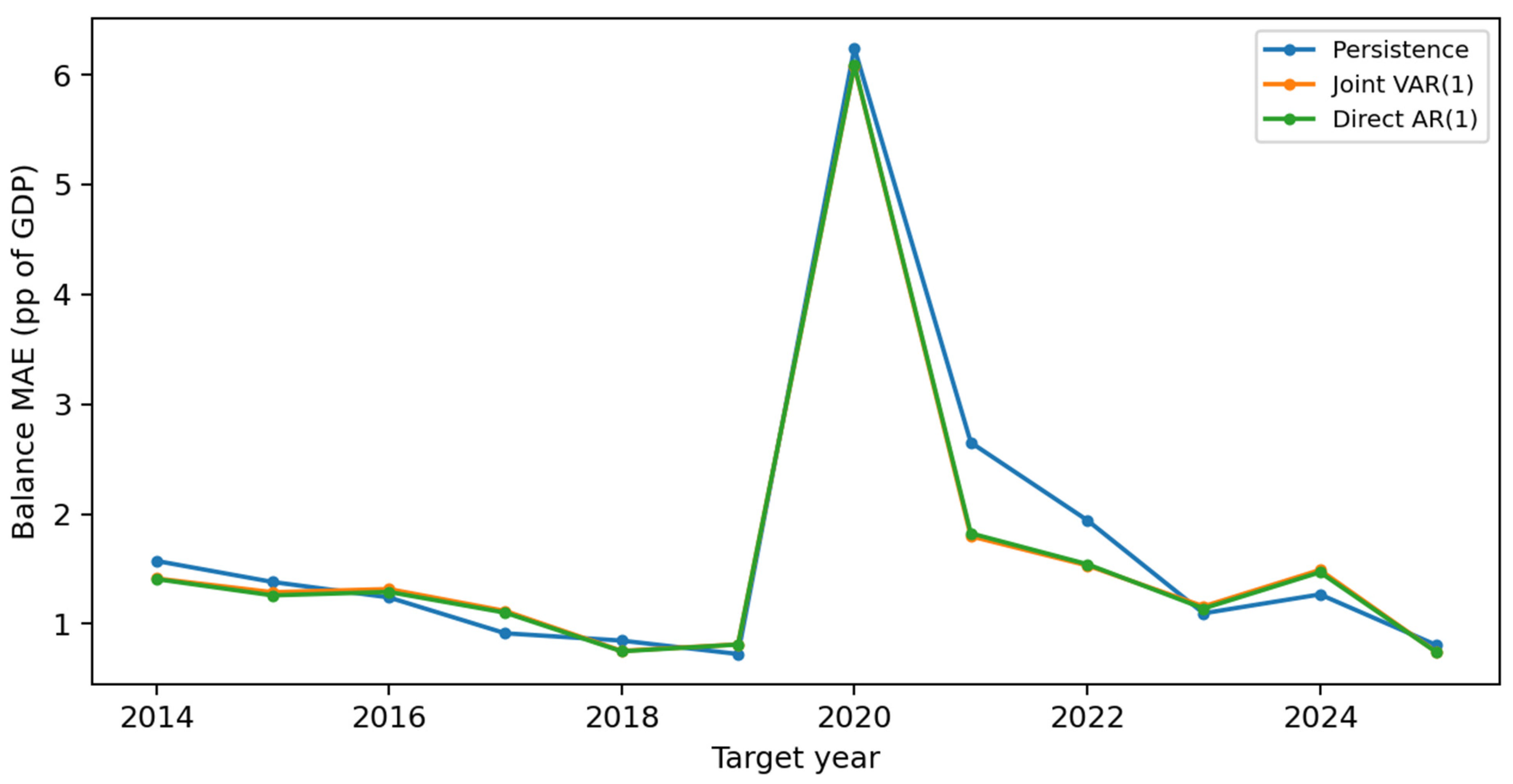
The joint advantage over persistence is concentrated in the crisis/recovery window. Excluding 2020–2022, joint-model MAE is 1.122 against 1.095 for persistence. Excluding 2021 alone reduces the joint advantage to approximately 0.030 percentage points. This is consistent with substantial reversion after the pandemic deficit shock rather than a general forecasting improvement in all regimes. Some individual non-crisis years favour the joint model, so the aggregate finding should not be paraphrased as failure in every ordinary year. Table 4 summarises the target-year subsets, and Table 5 reports block-bootstrap intervals for gains over persistence.
Table 4.
Balance MAE across target-year subsets.
Table 5.
Paired uncertainty for MAE gains over persistence.
The joint VAR interval includes zero once annual common shocks are preserved. Accordingly, we withdraw the suggestion that a narrowly positive country-only interval establishes robust superiority. The revised evidence supports a modest sample-average improvement with substantial temporal uncertainty. Table 6 compares the same forecast targets using the original and extended estimation histories.
Table 6.
Same targets with a longer training history.
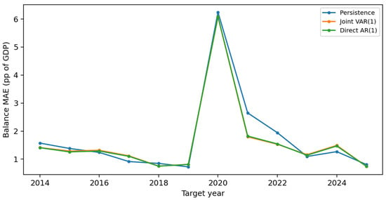
The longer history slightly improves direct AR(1) MAE but does not improve the pooled VAR(1). Tuned ridge is substantially better than the original fixed-penalty comparator, yet it does not beat the original direct AR(1). The evidence therefore concerns these particular models and training choices; it cannot sustain a universal statement that complexity or country heterogeneity is unhelpful. Figure 2 presents annual balance MAE for the original revised-data experiment.
Figure 2.
Annual balance MAE for the original revised-data experiment. The 2020 shock dominates absolute errors, while much of the joint-model advantage occurs during subsequent reversion. Source: Authors’ calculations based on Eurostat AGFS data (Eurostat, 2026).
4.3. Additional Macroeconomic Information
Lagged macroeconomic controls worsen rather than improve the matched balance forecasts. Joint VARX MAE is 1.695 versus 1.622 for its matched unaugmented model; direct ARX is 1.681 versus 1.620. These results reject the empirical expectation of lower sample MAE for these specific lagged-control extensions. They do not show that macroeconomic information is irrelevant: past macroeconomic values may contain little information about a future shock or forthcoming policy change. Table 7 reports the matched-sample comparison. Table 8 presents the separate archived-information experiment.
Table 7.
Matched-sample revised-data macroeconomic extension.
Table 8.
Archived autumn information and spring-after-target outcomes.
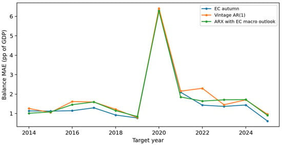
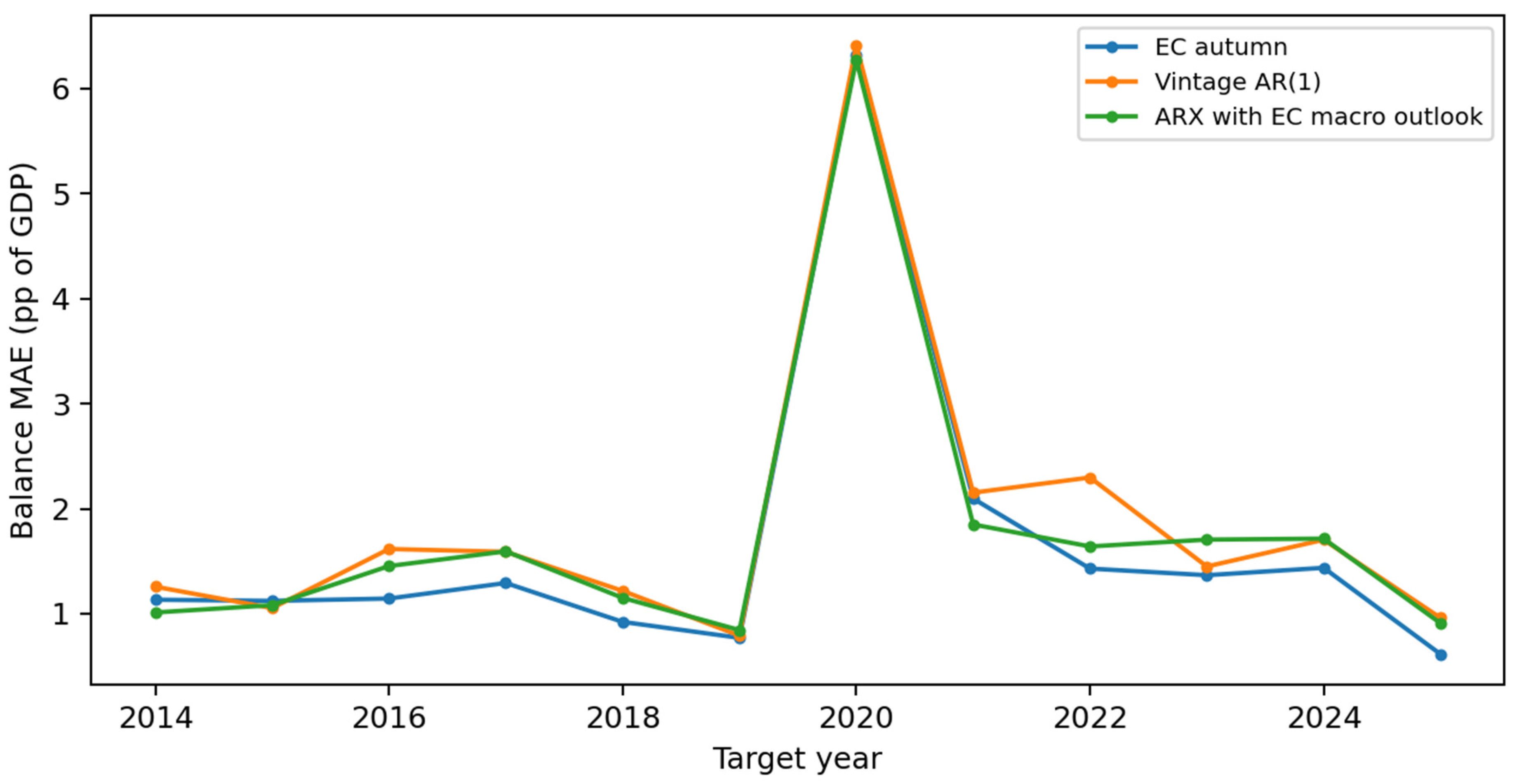
The origin-specific macroeconomic outlook improves the vintage direct AR from MAE 1.875 to 1.769, a reduction of 0.106 percentage points or approximately 5.6%. The two-year block interval for this gain is [0.003, 0.230] and the three-year interval is [0.010, 0.220]. The positive intervals are suggestive under these resampling assumptions, not a guarantee of future performance or a multiplicity-adjusted confirmatory result.
The EC’s own balance forecast is more accurate at MAE 1.637. It also outperforms the outlook-augmented ARX, whose MAE is higher by 0.132 percentage points. We therefore do not claim to replace the institutional forecast. The gain from forecasted growth and prices is consistent with the value of forward-looking information, while the remaining gap can reflect policy knowledge, richer information, or modelling differences. The present design does not separately identify those explanations.
The ranking persists when the earliest small training windows are omitted: for targets 2016–2025, MAE is 1.739 for EC, 1.914 for outlook ARX and 2.019 for AR; for 2017–2025, it is 1.805, 1.965 and 2.064, respectively. These checks address the earliest-origin concern but do not lengthen the time dimension or eliminate revision and measurement uncertainty in the archive. Figure 3 shows annual errors in the archived-information experiment.
Figure 3.
Annual errors in the archived-information experiment. EC is the autumn balance projection; the augmented ARX uses EC forecasts of real GDP growth and GDP-deflator growth available at the same origin. Source: Authors’ calculations based on the Forecast Tracker (European Fiscal Board Secretariat, 2026).
5. Discussion
RQ1 receives a conditional answer. Cross-series lags improve balance MAE over separate component autoregressions, but not over direct balance AR(1). The near-cancellation of coefficients explains why a two-equation system can produce a balance path close to a simple mean-reverting rule. Component scoring further limits the operational claim: the joint model does not improve both fiscal components over persistence. Its coherence is useful for presenting linked scenarios, but accuracy must be established separately.
RQ2 highlights the distinction between adding historical controls and adding a forward-looking information set. Lagged growth, prices, and interest expenditure do not help in the tested revised-data specifications. In the archived exercise, the same-origin macroeconomic outlook improves the direct model. This is compatible with the information-set motivation of Carriero et al. (2015), while differing from their large Bayesian and time-varying systems. It would be inappropriate to attribute our improvement to Bayesian shrinkage, structural change modelling, or causal channels that we did not estimate.
RQ3 shows that the original aggregate gain is sensitive to the pandemic/recovery period, and that country-only resampling understated temporal uncertainty. Longer estimation history and proper ridge tuning alter scores but do not reverse the central joint-versus-direct finding. This parallels the motivation for exceptional-period evaluation in Axioglou et al. (2025), without claiming numerical equivalence to institutional studies with different samples and forecast conventions.
The practical implication is to report separate component accuracy, retain a simple direct benchmark, and distinguish a mechanically coherent fiscal scenario from an operational forecast. The original improvement of 0.099 percentage points of GDP is approximately 5.7% of persistence MAE; the joint-versus-direct difference of about 0.007 is much smaller. These error differences should not be interpreted as guaranteed budget savings. Costs of forecast errors, asymmetric risks and implementation constraints are not estimated here.
Institutional comparisons must respect timing. Our archived model uses the Commission’s macroeconomic outlook, so its performance is conditional on that externally supplied input. The Commission’s own balance forecast has additional information and judgement, which is a legitimate practical advantage rather than a statistical defect of the benchmark. Beetsma et al. (2009), Frankel (2011), Büttner and Kauder (2009), and Chabin et al. (2020) collectively motivate separating planning, forecast production and evaluation rather than treating all predictions as interchangeable.
Limitations
The joint and revised-data macro experiments are retrospective tests using later releases. They are not genuine real-time joint-system evaluations. The archived direct extension improves temporal discipline but relies on a retrospectively assembled official archive, rounded values, and the archive’s historical conventions. GDP-deflator growth is derived from rounded nominal and real growth rates. Early origins have short training histories; later-start sensitivity checks reduce that concern but retain only a small number of target years.
There are only 12 evaluation years, common European shocks, potentially unstable relationships, and several reviewer-motivated comparisons. Block intervals preserve within-year dependence and short blocks of serial structure but cannot establish reliable inference under arbitrary regime change. No multiple-testing correction or new untouched validation period is available. Parameter tuning is nested within training windows, yet the overall choice to investigate these extensions followed inspection of the original evidence.
Country fixed effects may suffer short-T bias, and pooled coefficients suppress heterogeneity. We do not estimate a bias-corrected dynamic panel, a structural VAR, or a cointegrated system. The macroeconomic specifications omit explicit announced policy measures; the EC benchmark may incorporate them, but this does not identify their marginal contribution. Extending back to 1995 increases available training records without resolving breaks, revisions or nonstationarity. The results concern annual ratios, not nominal fiscal budgets, and should not be extrapolated mechanically to other countries or horizons.
6. Conclusions
This study distinguishes accounting coherence, cross-series dynamics and information timing in fiscal-balance forecasting for 27 present-day EU countries. The joint VAR improves on persistence and separate component autoregressions in the full revised-data sample, but direct balance AR(1) is slightly more accurate. Component results do not establish a general revenue-and-expenditure advantage, and the apparent gain over persistence is concentrated in pandemic/recovery years.
The expanded evidence changes the interpretation of complexity. Training-window ridge selection substantially improves the original penalised comparator, while lagged macroeconomic controls fail to improve matched-sample scores. A longer 1995–2025 estimation panel does not make the joint VAR uniformly better. These are results about tested specifications rather than a rejection of richer modelling in general.
In a separate archived-information exercise, forecasts of growth and prices available at the origin improve a direct fiscal-balance model, but the EC’s own balance forecast remains superior. The contribution is therefore a reproducible account of when added dynamics or information help and when they do not. Further operational validation should extend the joint system to complete historical release vintages, incorporate policy information explicitly, and evaluate future targets that were not used in developing the present revision.
Supplementary Materials
The following supporting information can be downloaded at https://www.mdpi.com/article/10.3390/economies14110558/s1. The accompanying package contains the source AGFS workbook, the official EFB Forecast Tracker workbook, the original replication program, the extension programs, derived panels, all forecast-level results, tuning choices, origin counts, component diagnostics, block intervals, sensitivity results, and figure files. Sources, retrieval dates, and checksums are documented. The original analysis was rerun from the source workbook, and its reported model MAEs were reproduced. The added analyses can be regenerated in the documented order. The original historical workbook’s filename date is not independently verified as an official publication date. Main-text Table 5, Table 6, Table 7 and Table 8 correspond to results/year_block_uncertainty.csv, results/revised_data_accuracy.csv (extended-history models), results/macro_accuracy.csv and results/vintage_accuracy.csv, respectively. The underlying forecast-level records are provided in results/all_revised_data_forecasts.csv, results/macro_forecasts.csv and results/vintage_forecasts.csv; tuning records are in results/ridge_inner_validation.csv. Reproduction instructions are provided in README_REPLICATION.txt.
Author Contributions
Conceptualization, I.M. and N.P.; methodology, I.M. and N.P.; software, I.M. and N.P.; validation, I.M. and N.P.; formal analysis, I.M. and N.P.; data curation, I.M. and N.P.; writing—original draft preparation, I.M. and N.P.; writing—review and editing, I.M. and N.P. All authors have read and agreed to the published version of the manuscript.
Funding
This research received no external funding.
Institutional Review Board Statement
Not applicable.
Informed Consent Statement
Not applicable.
Data Availability Statement
The data sources are Eurostat’s Government revenue, expenditure and main aggregates (gov_10a_main; https://ec.europa.eu/eurostat/databrowser/product/page/GOV_10A_MAIN, accessed on 21 October 2026) and the European Fiscal Board Secretariat’s Forecast Tracker (https://commission.europa.eu/european-fiscal-board-efb/forecast-tracker_en, accessed on 2 November 2026). The accompanying replication package described in the Supplementary Materials section contains the source workbooks, derived panels, analysis programs, forecast-level results and reproduction instructions.
Acknowledgments
During preparation of this manuscript, the authors used ChatGPT (GPT-5.6, OpenAI) to assist with editorial drafting, formatting, and development of analysis code. The authors are responsible for reviewing the analysis, references, and final manuscript and for the content submitted for publication.
Conflicts of Interest
The authors declare no conflicts of interest.
Appendix A. Diagnostics and Secondary Indicators
The original pooled equations exhibit expenditure heteroskedasticity and non-normal residuals. Breusch–Pagan p-values are 0.128 for revenue and 0.0000874 for expenditure; White p-values are 0.161 and 0.000000129. Shapiro–Wilk rejects normality in both equations, while RESET p-values are 0.101 and 0.015. Within-country residual-lag regressions give p-values of 0.826 and 0.110. These are descriptive checks on full-sample fits, not proof of forecast validity. They neither justify an across-country Durbin–Watson calculation nor remove common-year dependence.
The exploratory 2025 MCD screen uses revenue, expenditure and their annual changes, with MinCovDet random_state=5324, support_fraction=None and assume_centered=False (Rousseeuw & Van Driessen, 1999). Its raw and reweighted support sizes are 16 and 20. A chi-square reference with four degrees of freedom flags seven countries at the 97.5th percentile: Ireland, Cyprus, Greece, Romania, Denmark, Poland and Belgium. This small-sample heuristic is not a formal test of country data errors. It is not used for model selection or principal forecast evaluation; no flagged country is removed. The original retrospective exclusion comparison is retained only in the reproduction files and has no role in the revised conclusions.
The coverage indicator is 100r/e, and its model projection is 100. It is a ratio of component forecasts, not generally an unbiased estimate of E[100r/e | information]. It also equals 100(1 + b/e), so it is mechanically linked to the balance and expenditure denominator rather than an independent validation target. Coverage results remain in the Supplementary Materials as a secondary operational description, with no separate claim of new predictive information.
References
- Afonso, A., & Coelho, J. C. (2022). Fiscal sustainability, fiscal reactions, pitfalls and determinants (CESifo Working Paper No. 9635). Available online: https://www.ifo.de/en/cesifo/publications/2022/working-paper/fiscal-sustainability-fiscal-reactions-pitfalls-and-determinants (accessed on 9 November 2026).
- Axioglou, C., Ratto, M., & Roman, J. (2025). Navigating uncertainty: Evaluating the European economic forecasts amidst pandemic and energy crises (European Economy Discussion Paper 222). European Union. [Google Scholar] [CrossRef]
- Beetsma, R., Giuliodori, M., & Wierts, P. (2009). Planning to cheat: EU fiscal policy in real time. Economic Policy, 24(60), 753–804. [Google Scholar] [CrossRef] [Scilit]
- Büttner, T., & Kauder, B. (2009). Revenue forecasting practices: Differences across countries and consequences for forecasting performance (CESifo Working Paper 2628). Available online: https://www.ifo.de/en/cesifo/publications/2009/working-paper/revenue-forecasting-practices-differences-across-countries-and (accessed on 9 November 2026).
- Carriero, A., Mumtaz, H., & Theophilopoulou, A. (2015). Macroeconomic information, structural change, and the prediction of fiscal aggregates. International Journal of Forecasting, 31(2), 325–348. [Google Scholar] [CrossRef] [Scilit]
- Chabin, A., Lamproye, S., & Výškrabka, M. (2020). Are we more accurate? Revisiting the European Commission’s macroeconomic forecasts (European Economy Discussion Paper 128). European Union. [Google Scholar] [CrossRef]
- Ćurčić, M. (2025). Legal and economic analysis of public expenditures in conditions of budget limitations. The Financial Advisor, 30(1), 75–93. https://fa-journal.com/index.php/fa/article/view/4.
- European Central Bank. (n.d.). What is the general government balance? Available online: https://data.ecb.europa.eu/methodology/what-general-government-balance (accessed on 21 October 2026).
- European Commission, Directorate-General for Economic and Financial Affairs. (2016). Measuring the uncertainty in predicting public revenue (European Economy Discussion Paper 39). European Union. [Google Scholar] [CrossRef]
- European Fiscal Board Secretariat. (2026). Forecast tracker [Data set and methodology]. European Commission. Available online: https://commission.europa.eu/european-fiscal-board-efb/forecast-tracker_en (accessed on 2 November 2026).
- Eurostat. (2026). Government revenue, expenditure and main aggregates (gov_10a_main) [Data set]. Available online: https://ec.europa.eu/eurostat/databrowser/product/page/GOV_10A_MAIN (accessed on 21 October 2026).
- Frankel, J. A. (2011). Over-optimism in forecasts by official budget agencies and its implications. Oxford Review of Economic Policy, 27(4), 536–562. [Google Scholar] [CrossRef] [Scilit]
- Hyndman, R. J., & Koehler, A. B. (2006). Another look at measures of forecast accuracy. International Journal of Forecasting, 22(4), 679–688. [Google Scholar] [CrossRef] [Scilit]
- Milanović, N. (2022). Linkage of internal controls and audits in the public sector. The Financial Advisor, 27(1), 65–75. [Google Scholar] [CrossRef] [Scilit]
- Nickell, S. (1981). Biases in dynamic models with fixed effects. Econometrica, 49(6), 1417–1426. [Google Scholar] [CrossRef] [Scilit]
- Pešić, H., & Miljković, M. (2020). Održivost budžetskih načela i procedura [Sustainability of budget principles and procedures]. Održivi razvoj, 2(2), 15–29. [Google Scholar] [CrossRef] [Scilit]
- Petropoulos, F., Apiletti, D., Assimakopoulos, V., Babai, M. Z., Barrow, D. K., Ben Taieb, S., Bergmeir, C., Bessa, R. J., Bijak, J., Boylan, J. E., Browell, J., Carnevale, C., Castle, J. L., Cirillo, P., Clements, M. P., Cordeiro, C., Oliveira, F. L. C., De Baets, S., Dokumentov, A., … Ziel, F. (2022). Forecasting: Theory and practice. International Journal of Forecasting, 38(3), 705–871. [Google Scholar] [CrossRef] [Scilit]
- Politis, D. N., & Romano, J. P. (1991). A circular block-resampling procedure for stationary data (Technical Report). Department of Statistics, Stanford University. Available online: https://statistics.stanford.edu/technical-reports/circular-block-resampling-procedure-stationary-data (accessed on 9 November 2026).
- Rousseeuw, P. J., & Van Driessen, K. (1999). A fast algorithm for the minimum covariance determinant estimator. Technometrics, 41(3), 212–223. [Google Scholar] [CrossRef]
- Škrbić, S., Malešić, S., & Gojkov, D. (2023). Budget planning process. The Journal Law Review of Public Sector, 3(2), 21–35. [Google Scholar] [CrossRef] [Scilit]
- Škrbić, S., & Obrić, B. (2024). Budgetary and legal analysis of defense expenditure financing. The Journal Law Review of Public Sector, 4(1), 7–22. [Google Scholar]
- Tashman, L. J. (2000). Out-of-sample tests of forecasting accuracy: An analysis and review. International Journal of Forecasting, 16(4), 437–450. [Google Scholar] [CrossRef] [Scilit]

Disclaimer/Publisher’s Note: The statements, opinions and data contained in all publications are solely those of the individual author(s) and contributor(s) and not of MDPI and/or the editor(s). MDPI and/or the editor(s) disclaim responsibility for any injury to people or property resulting from any ideas, methods, instructions or products referred to in the content. |
© 2026 by the authors. Licensee MDPI, Basel, Switzerland. This article is an open access article distributed under the terms and conditions of the Creative Commons Attribution (CC BY) license.