


Abstract
This study investigates the long-term dynamic relationship between economic growth and greenhouse gas (GHG) emissions in Mongolia over the period 2010–2050 using an integrated System Dynamics modeling framework. The model endogenously couples macroeconomic production across 18 economic sectors via Cobb–Douglas production functions with sectoral energy demand, IPCC-compliant emission intensity, and a detailed 14-species forest carbon sequestration engine. Economic output is reported as nominal Gross Domestic Product (GDP) at current prices. The Tapio decoupling index, calculated annually from nominal GDP and gross GHG emissions, is used to assess the evolving elasticity between economic expansion and environmental pressure under three policy pathways: Business as Usual (BAU), Mitigation (S2, aligned with Mongolia’s NDC 3.0 and LT-LEDS incorporating 3533 MW across 32 energy projects), and Transformational (S3). The simulation results indicate that under the BAU scenario, nominal GDP reaches MNT 501.84 trillion by 2050, with gross GHG emissions escalating to MtCO2e and net GHG emissions reaching MtCO2e due to declining forest sequestration ( MtCO2e). Conversely, the Transformational scenario—combining aggressive clean energy expansion (1733 MW of hydro, solar, wind, and storage), legacy thermal plant decommissioning (220 MW), industrial electrification, and active forest ecosystem management—maintains equivalent economic output (nominal GDP of MNT 501.80 trillion) while reducing net GHG emissions to MtCO2e by 2050. This represents a 47.1% reduction in net GHG emissions relative to BAU. Furthermore, Tapio elasticity analysis reveals that while short-term structural investments in baseload power infrastructure, renewable grid expansion, and industrial capacity buildouts cause a temporary surge in emission intensity during 2028–2029 (expansive negative decoupling, ), the Transformational pathway uniquely achieves sustained absolute decoupling (, ranging between and ) throughout 2041–2050. These quantitative findings demonstrate that structural and technological transitions can successfully decouple economic expansion from emissions in resource-dependent, landlocked developing economies.
1. Introduction
1.1. Research Background
Climate change mitigation is increasingly becoming an integral part of long-term economic development rather than a policy objective that can be considered separately from economic growth. Changes in the scale and composition of economic activity affect energy demand, fuel use, investment, technological adoption, and, consequently, greenhouse gas (GHG) emissions. Conversely, improvements in energy efficiency, technological upgrading, electrification, the expansion of low-carbon energy sources, and structural shifts toward higher-value economic activities can reduce the GHG emission intensity of production. The central challenge is therefore not simply whether economic growth should continue, but whether the underlying drivers and mechanisms of growth can evolve so that increases in economic output are accompanied by a sustained reduction in environmental pressure. This relationship is inherently dynamic because economic structure, technology, energy systems, and environmental conditions interact and change over time.
This issue is particularly relevant to Mongolia because its economic structure is strongly influenced by mining and other resource-intensive activities, while its energy system remains heavily reliant on fossil fuels. This structural and energy system configuration contributes to a close relationship between economic activity, energy demand, and GHG emissions, highlighting the importance of examining how structural and technological transformation can support lower-emission economic growth. At the same time, Mongolia has progressively strengthened its climate commitments through its nationally determined contributions (NDCs). Under NDC 2.0, Mongolia identified an unconditional GHG emission reduction potential of 22.7% relative to the Business-as-Usual (BAU) pathway by 2030, with a conditional reduction potential of 27.2%. NDC 3.0, submitted in 2025, further strengthened the unconditional reduction targets to 23.0% by 2030 and 30.3% by 2035 (Government of Mongolia, 2025). These commitments increase the need to reconcile GHG emission reduction with continued economic development.
The relationship between economic growth and GHG emissions is not unidirectional. Expansion of production in energy- and resource-intensive sectors, including mining, energy, transport, agriculture, and construction, can increase energy and fuel demand and thereby increase GHG emissions. Conversely, technological innovation, improvements in energy efficiency, electrification, changes in the energy mix, and structural transformation within these sectors can reduce emissions per unit of economic output. The resulting trajectory therefore depends not only on the rate of economic growth but also on how production is organized, which technologies are adopted, how energy is supplied, and how the sectoral structure of the economy evolves over time.
For Mongolia, the key research issue is therefore not whether economic growth should be constrained to achieve emission reductions, but whether the structural and technological drivers of economic growth can be transformed so that economic expansion becomes progressively less GHG-intensive. Addressing this question requires an analytical framework that captures the interactions among economic growth, sectoral structure, technological change, energy demand, GHG emissions, and carbon sequestration over time.
1.2. Research Objective
The objective of this study is to develop and apply an integrated System Dynamics model to examine the long-term interactions among economic growth, energy use, GHG emissions, and forest carbon sequestration in Mongolia over the period 2010–2050. The model represents production across 18 economic sectors and links key socioeconomic drivers, including population, labor, capital accumulation, and technological change, with sectoral production, energy demand, GHG emissions, and forest carbon sequestration. Within this integrated framework, three alternative development pathways (Business as Usual (BAU), Mitigation, and Transformational) are formulated to examine how differences in mitigation measures, technological change, energy system transformation, and structural change may influence the relationship between economic growth and GHG emissions.
The study is guided by the following research question.
To what extent can structural and technological transformation enable Mongolia to maintain economic growth while reducing the GHG emission intensity of economic activity and its associated net GHG emissions through 2050?
To address this research question, the three development pathways are compared in terms of economic output (measured by nominal GDP in trillion MNT at current prices; see Section 3.3), gross GHG emissions, forest carbon sequestration, and the resulting net GHG balance. The Tapio decoupling index is additionally used to characterize changes in the relationship between economic growth and GHG emissions over time and to assess whether economic expansion becomes progressively less emission-intensive under alternative development pathways. Accordingly, the analysis considers both changes in the level of GHG emissions and changes in the relationship between economic activity and environmental pressure over the simulation period.
1.3. Research Contributions
The main contribution of this study is the integration of economic growth, energy use, GHG emissions, and forest carbon sequestration within a single System Dynamics framework to evaluate how structural and technological transformation may shape Mongolia’s long-term low-emission development pathway. The study contributes to the existing literature in four main respects.
- 1.
- Methodological Expansion of Forest Carbon Modeling (3 to 14 Species): Building directly upon the authors’ foundational dynamic model of Mongolia’s forest resources (Tumurbaatar et al., 2025), which was restricted to the growth dynamics and carbon stock of the 3 most dominant tree species, this study extends the biological growth equations and inventory data to cover 14 tree species. This expansion allows for a comprehensive, nationwide accounting of total forest stock and forest carbon sequestration potential.
- 2.
- Integration of an 18-Sector Production Dynamic with GHG Emissions: The extended forest module is endogenously coupled with a macroeconomic model representing production across 18 economic sectors. Cobb–Douglas production functions link labor, capital accumulation, and total factor productivity (TFP) with sectoral economic output (measured as nominal GDP), which subsequently drives energy demand and emission intensity across 5 major IPCC sectors (energy, transport, IPPU, agriculture, and waste).
- 3.
- Establishment of a National Net GHG Balance Framework: Rather than analyzing gross emissions or forestry sinks in isolation, the integrated System Dynamics framework subtracts total forest carbon sequestration from gross multi-sector emissions to derive Mongolia’s long-term net GHG balance through 2050.
- 4.
- Comparative Scenario Analysis and Decoupling Evaluation: The study formulates and simulates three distinct development pathways—Business as Usual (BAU), Mitigation (NDC 3.0), and Transformational—evaluating long-term economic expansion, net emission trajectories, and structural decoupling using the Tapio decoupling index.
2. Literature Review and Theoretical Framework
2.1. Production Functions and Economic Growth Theory
Economic growth theory generally explains changes in output through the accumulation and productivity of production factors, particularly capital and labor, together with improvements in TFP. Cobb and Douglas (1928) introduced a production function relating manufacturing output to capital and labor inputs, providing an analytical basis for examining the contribution of factor accumulation and technological change to production growth. The Cobb–Douglas production function subsequently became a widely used specification in economic growth analysis and macroeconomic modeling (Mankiw et al., 1992; Solow, 1956).
In the context of environmental economics, traditional growth models have been extended to incorporate resource depletion and environmental degradation. The “Green Solow Model” formulated by Brock and Taylor (2010) demonstrates that continuous technological progress and efficiency improvements are necessary conditions for reconciling long-term economic expansion with environmental sustainability. Furthermore, empirical macroeconomic research underscores that substituting carbon-intensive capital with clean energy technologies and enhancing energy-oriented TFP can suppress the emission intensity of aggregate production without compromising economic output (Acemoglu et al., 2012; Jorgenson et al., 2014).
In the present study, the production function provides the basis for representing the relationship between socioeconomic drivers and sectoral economic output. Capital accumulation and labor supply are represented as the principal production factors, while technological and organizational improvements are incorporated through total factor productivity. This formulation makes it possible to connect changes in the scale and composition of economic activity with subsequent changes in energy demand and GHG emissions within the System Dynamics framework.
2.2. Economic Growth, GHG Emissions, and Decoupling
Economic growth can increase environmental pressure through higher demand for energy, fuels, transportation, and material inputs. However, the relationship between economic activity and environmental pressure is not necessarily proportional. Improvements in energy efficiency, technological change, electrification, changes in the energy mix, and structural transformation toward less emission-intensive activities can reduce the amount of GHG emissions associated with a given level of economic output. This changing relationship between economic activity and environmental pressure is commonly examined through the concept of decoupling (OECD, 2002; UNEP, 2011).
Tapio (2005) developed a quantitative framework for characterizing the relationship between changes in economic activity and changes in environmental pressure through the decoupling index. The index expresses the relative change in environmental pressure in relation to the relative change in economic activity and can be expressed as follows:
where denotes the decoupling index, represents the relative change in gross GHG emissions, and represents the relative change in nominal GDP over the corresponding period (Tapio, 2005).
The Tapio decoupling framework has been widely applied to evaluate the environmental sustainability of economic development across various spatial and sectoral scales. For instance, empirical studies in emerging and resource-dependent economies demonstrate that while rapid industrialization initially drives expansive negative decoupling (), targeted structural adjustments, renewable energy integration, and stringent energy efficiency mandates can successfully shift economies toward weak () and eventually strong or absolute decoupling () (Tapio, 2005). However, literature also warns that decoupling achieved in high-income economies is frequently offset by embodied carbon flows in international trade or short-term infrastructure boom cycles (Hubacek et al., 2021).
The conceptual distinction between relative and absolute decoupling is central to the Tapio framework. Relative decoupling occurs when economic output and environmental pressure increase simultaneously, but environmental pressure increases more slowly than economic output. Absolute decoupling occurs when economic output increases while environmental pressure decreases. Conversely, when environmental pressure increases faster than economic output, the relationship indicates a negative-decoupling condition. The framework also distinguishes recessive states in which both economic activity and environmental pressure decline, because an emission reduction occurring together with economic contraction does not necessarily represent an improvement in the environmental performance of economic growth (Tapio, 2005).
Decoupling should be distinguished from a reduction in emission intensity and from an improvement in the net GHG balance. A declining GHG emission intensity indicates that fewer emissions are generated per unit of economic output, whereas decoupling characterizes the relative change between economic activity and environmental pressure over a specified period. Similarly, decoupling is not equivalent to achieving a lower net GHG balance or net-zero emissions, because the Tapio index is based on the relationship between changes in GDP and gross GHG emissions and does not directly incorporate carbon sequestration. Therefore, a pathway may exhibit relative or even absolute decoupling while still maintaining a substantial level of gross or net GHG emissions.
In the present study, the Tapio framework is applied to characterize the annual relationship between nominal GDP and gross GHG emissions under the BAU, Mitigation, and Transformational development pathways. The index is used as a complementary indicator of the changing emission response to economic growth rather than as a direct measure of total emission performance or policy effectiveness. The decoupling results are therefore interpreted jointly with gross GHG emissions, GHG emission intensity, forest carbon sequestration, and the resulting net GHG balance. This combined interpretation allows for the study to distinguish between a weakening of the annual emission response to economic growth and an actual reduction in the overall GHG burden of the economy.
2.3. System Dynamics and Integrated Socioeconomic–Environmental Modeling
The foundational contributions of Forrester (1961) and Sterman (2000), together with the early applications of systems thinking to global socioeconomic and environmental problems by Meadows et al. (1972), established an important basis for the use of System Dynamics in representing complex interactions among socioeconomic, technological, and environmental processes.
The relevance of System Dynamics to climate–economic analysis arises from the interdependence among economic production, energy demand, technological change, environmental pressure, and policy responses. Integrated System Dynamics models have been developed to represent interactions among economy, energy, climate, society, and environmental systems. Early System Dynamics applications to climate economics, such as Fiddaman’s FREE model (Fiddaman, 2002), highlighted the critical role of feedback loops, capital inertia, and technological delays in energy transitions. Subsequent macro-environmental dynamic modeling frameworks, including World-3 updates and En-ROADS, have further substantiated that non-linear feedback mechanisms are indispensable for evaluating long-term climate-policy interactions (Herrington, 2021; Rooney-Varga et al., 2020).
The Akhtar et al. (2013) integrated assessment framework links society, biosphere, climate, economy, and energy within a feedback-based System Dynamics structure and uses alternative policy scenarios to examine interactions among model subsystems. More recent applications have extended System Dynamics to economy–energy–environment systems at the regional level. For example, an energy–economy–environment System Dynamics model for Inner Mongolia represents economic activity by sector and simultaneously accounts for energy consumption, carbon emissions, carbon intensity, and vegetation-based carbon sequestration (Zhu et al., 2024). Similarly, recent carbon pathway studies have integrated economic, technological, population, industrial, and environmental subsystems and have incorporated carbon absorption alongside emissions in scenario-based System Dynamics models (Dong et al., 2025).
These studies demonstrate the value of integrated dynamic modeling, but they also indicate that the specific model architecture and system boundary remain important. Models may differ substantially in the degree to which economic production is endogenous, the level of sectoral disaggregation, the treatment of energy demand, and the representation of natural carbon sinks. The present study therefore focuses specifically on linking sectoral production dynamics, energy demand, GHG emissions, and forest carbon sequestration within a Mongolia-specific long-term framework.
2.4. Energy–Economy–Environment Linkages and Carbon Sequestration
A substantial body of integrated assessment research has linked economic and energy systems with land-use and forestry components. For example, the World Induced Technical Change Hybrid (WITCH) energy–economy–climate model has been linked with the Global Timber Model (GTM) to examine the role of forestry in climate mitigation and the interaction between forest sequestration and energy-sector mitigation (Tavoni et al., 2007). Similarly, research integrating land-use and energy-sector perspectives has shown that biological carbon sequestration can interact with energy system mitigation strategies, particularly where biomass and land-use decisions are relevant to climate policy (Bauer et al., 2020).
In land-use and forest carbon dynamics modeling, advanced dynamic growth frameworks emphasize that biological carbon sinks are non-linear, age-dependent, and highly sensitive to climate stress and disturbance regimes (Friedlingstein et al., 2022). Integrating natural terrestrial sinks into macroeconomic optimization or dynamic simulation models provides a complete perspective on net emission balance, enabling policymakers to balance technological abatement costs with natural ecosystem conservation investment (Fuss et al., 2018).
At the regional level, System Dynamics studies have also incorporated forest or vegetation carbon sinks into economy–energy–environment models. For example, a System Dynamics model for the Beijing–Tianjin–Hebei region includes GDP, energy consumption, technology investment, carbon emissions, forest area, and forest carbon sequestration within a scenario-based framework (Zeng et al., 2023). These studies provide evidence that carbon sinks can be incorporated into dynamic economy–energy–environment models, while also highlighting the importance of defining the mechanisms through which economic activity, investment, environmental management, and carbon sequestration are connected.
2.5. Mongolia-Specific Research and Existing Modeling Approaches
Mongolia-specific studies have examined the relationship between economic activity, energy use, and GHG emissions using different analytical approaches. The Global Green Growth Institute (2021)-supported national assessment developed baseline and mitigation projections for Mongolia to 2050 and identified the energy sector, particularly electricity and heat production, as a major source of future emissions under the baseline pathway. The assessment also evaluated mitigation measures involving renewable energy, energy efficiency, and transport (Global Green Growth Institute, 2021).
More recently, long-term GHG mitigation pathways for Mongolia have been developed using sector-specific energy and emission calculations. The study projects emissions under baseline and mitigation pathways to 2050 and provides a detailed representation of energy demand across residential, industrial, commercial and public services as well as transport, and agriculture, forestry and fishing. However, its approach is primarily based on sectoral activity variables and energy intensities rather than an endogenous multi-sector production system linking capital, labor, and technological change to economic output (Namkhainyam et al., 2024).
Another recent study applied an environmentally extended input–output model together with Structural Decomposition Analysis and Structural Path Analysis to identify the sectoral drivers and transmission pathways of Mongolia’s energy-related carbon emissions. This approach provides important evidence on the structural sources of emissions and the inter-sectoral transmission of embodied emissions, but it is primarily retrospective and decomposition-based rather than a forward-looking dynamic simulation of endogenous economic production and forest carbon sequestration (Ma et al., 2025).
Taken together, these studies provide important empirical and scenario-based evidence regarding the challenges of decarbonization in Mongolia. Nevertheless, they differ from the present study in system boundary, methodological structure, and treatment of long-term feedbacks. In particular, existing Mongolia-focused studies do not simultaneously represent an 18-sector production system based on capital, labor, and technological change, sector-linked energy demand and GHG emissions, and a dynamic forest carbon sequestration module within a single System Dynamics framework.
2.6. Research Gap and Analytical Positioning
The literature indicates that several components relevant to low-emission development have already been studied extensively, including production and economic growth, energy–economy–environment interactions, GHG emissions and decoupling, and forest carbon sequestration. Integrated assessment models have also demonstrated the feasibility of linking economic, energy, climate, and land-use systems. Therefore, the research gap addressed by this study should not be understood as the absence of integrated models in the international literature.
Rather, the gap concerns the specific integration and application of these components to Mongolia’s long-term development dynamics. Three dimensions are particularly relevant.
First, Mongolia-specific studies have examined energy use and GHG emissions through baseline and mitigation scenarios or through structural decomposition, but relatively less attention has been given to an endogenous multi-sector production structure in which capital accumulation, labor, and technological change jointly determine sectoral output and subsequently influence energy demand and GHG emissions (Ma et al., 2025; Namkhainyam et al., 2024).
Second, international integrated assessment studies have demonstrated the value of linking energy–economy dynamics with forestry, land-use, and carbon-cycle processes (Akhtar et al., 2013; Tavoni et al., 2007). However, existing Mongolia-focused modeling architectures have largely evaluated economic expansion, sectoral energy demand, and biological carbon sinks in isolation. The present study addresses this fragmentation by directly expanding the authors’ foundational System Dynamics forest model (Tumurbaatar et al., 2025) and embedding it within a fully coupled macro-environmental framework.
To explicitly clarify the incremental contributions of this manuscript relative to Tumurbaatar et al. (2025), Table 1 details the specific structural, parametric, and domain-level advancements carried forward versus newly developed.
Table 1.
Structural, domain, and data boundary comparison between the previous forest model (Tumurbaatar et al., 2025) and the present integrated System Dynamics framework.
Third, as outlined in Table 1, the present framework fully accounts for gross emissions across all five IPCC sectors—including non- gases such as methane () and nitrous oxide () from livestock, fugitive coal mining, and waste, expressed in MtCO2e using IPCC GWP-100 values. In terms of biological sinks, the model dynamically captures living forest sequestration () across 14 tree species, endogenously accounting for annual growth increments alongside losses from forest fires and pest infestations based on Tumurbaatar et al. (2025). However, biological carbon sequestration from pastureland biomass and soil organic carbon (SOC) remains outside the model boundary. In Mongolia’s arid rangelands, pasture soil carbon fluxes exhibit extreme interannual volatility driven by overgrazing, desertification, and harsh winter conditions (dzud), causing grassland soils to fluctuate unpredictably between weak sinks and net emission sources. Excluding grassland soil sinks aligns with the IPCC conservative accounting principle, avoiding artificial over-crediting of unmanaged terrestrial sinks and ensuring that the resulting forest-adjusted net GHG balance serves as a reliable metric for long-term policy evaluation.
Accordingly, the analytical contribution of this study lies in combining an 18-sector production structure, socioeconomic drivers, energy demand, GHG emissions, forest carbon sequestration, alternative climate pathways, and three development pathways within a single System Dynamics framework for Mongolia over 2010–2050. The framework is subsequently used to evaluate economic output, gross GHG emissions, forest carbon sequestration, net GHG balance, and the changing growth–emission relationship through the Tapio decoupling index.
3. Materials and Methods
3.1. System Boundary of the Study
The System Dynamics model developed in this study integrates the socioeconomic, economic, energy, environmental, and climate dimensions of Mongolia’s long-term development (Figure 1). The model represents the interactions among population, labor, capital accumulation, sectoral production, energy demand, GHG emissions, climate-related effects, forest carbon sequestration, and alternative economic and policy development pathways (S1–S3). Reinforcing loops (R) represent mechanisms that amplify changes within the system, whereas balancing loops (B) represent mechanisms that counteract or constrain changes. The principal feedback structures shown in Figure 1 represent (i) growth-supporting socioeconomic and production dynamics, (ii) climate-related effects on productivity and environmental conditions, and (iii) interactions among policy measures, technological change, GHG emissions, and economic decoupling.
Figure 1.
Structural framework of the System Dynamics model. R denotes reinforcing loops and B denotes balancing loops. Solid, dashed, and dotted links indicate direct, indirect, and supporting relationships, respectively.
The solid links in the structural diagram indicate variables that directly enter the production mechanism, particularly capital and labor, whereas dashed links represent factors that affect production or other system components indirectly through productivity, climate conditions, or policy pathways. Dotted links indicate relationships that are relevant to the system but do not constitute the principal causal flow of the model (Figure 1).
The model consists of interconnected socioeconomic, economic, energy, environmental, and climate-related subsystems. The socioeconomic subsystem includes population, labor force, unemployment, poverty, and the Human Development Index (HDI). The economic subsystem represents value added across 18 economic sectors. The energy subsystem represents sectoral energy demand and changes in the energy mix. The environmental subsystem incorporates forest resources and carbon sequestration together with agriculture and waste-related processes. Climate-related variables, including precipitation, temperature, and drought conditions, are incorporated as external pathway-dependent drivers that affect relevant environmental and production processes.
The simulation period covers 2010–2050. The period 2010–2025 represents the historical and model calibration period, while 2026–2050 represents the scenario simulation period. Gross Domestic Product (GDP) is calculated using the production approach as the sum of value added across the 18 economic sectors and is reported at current prices (nominal GDP; see Section 3.3). GHG emissions are estimated using sector-specific activity and emission relationships consistent with the 2006 IPCC Guidelines for National Greenhouse Gas Inventories and their 2019 Refinement Intergovernmental Panel on Climate Change (2006, 2019), and are aggregated into five major source groups: energy, transport, agriculture, industrial processes, and waste.
The forest carbon sequestration component of the present model builds upon and significantly extends the authors’ previously developed Mongolia-specific System Dynamics framework of forest fund dynamics (Tumurbaatar et al., 2025). That foundational model captured dynamic alterations in Mongolia’s forest area and standing volume across major tree species, integrating localized microclimate drivers (precipitation, temperature, drought severity, and soil moisture dynamics) alongside disturbance regimes including forest fires and pest infestations through biological stress feedback loops. The present study embeds this dynamic forest sequestration engine () directly into the multi-sector macroeconomic and energy system architecture.
In this integrated dynamic framework, forest carbon sequestration is evaluated in conjunction with total gross national emissions to establish the forest-adjusted net GHG balance. Mathematically, the net GHG balance in year t () is formulated as
where denotes total gross national GHG emissions across all five core IPCC inventory sectors (energy, industrial processes and product use [IPPU], agriculture, transport, and waste). Crucially, comprehensively incorporates both direct carbon dioxide () and major non- greenhouse gases—specifically enteric and fugitive methane () and agricultural nitrous oxide ()—converted into carbon dioxide equivalents (MtCO2e) using IPCC Global Warming Potentials (GWP-100).
The term represents annual net atmospheric carbon removal by living forest biomass across 14 species classes. In accordance with IPCC Good Practice Guidance for Land Use, Land-Use Change and Forestry (LULUCF), endogenously accounts for annual biomass growth increments minus natural losses, incorporating disturbance-induced carbon releases from forest fires and pest-driven mortality modeled in Tumurbaatar et al. (2025).
It is methodologically important to clarify that in Equation (2) represents a forest-adjusted net GHG balance rather than a complete LULUCF national net inventory. Grassland biomass and soil organic carbon (SOC) dynamics are excluded from . In Mongolia’s arid and semi-arid ecosystems, grassland carbon fluxes exhibit extreme interannual variance driven by desertification, overgrazing, and severe winter weather (dzud), causing pasture soils to shift frequently between weak sinks and net carbon sources. Under a conservative accounting framework, excluding uncertain soil and grassland fluxes avoids over-crediting natural sinks, ensuring that serves as a robust, conservative indicator for evaluating the true mitigation efficacy of alternative national development pathways.
Thus, the present study does not evaluate the forest sector as an isolated ecological unit; rather, it embeds dynamic forest sequestration within a coupled macroeconomic–energy–environmental feedback architecture. This enables the model to trace non-linear interactions among demographic dynamics, factor accumulation, sectoral Cobb–Douglas output, technological intensity, structural energy demand, IPCC-compliant multi-gas emissions, and dynamic biological carbon sinks over the 2010–2050 simulation horizon.
3.2. Cobb–Douglas Production Function
Sectoral economic output is represented using a Cobb–Douglas production function. For sector i in year t, output is specified as
where denotes the annual output or value added of sector i in year t; represents TFP, capturing technological development, organizational efficiency, innovation, and other productivity-enhancing factors not explicitly represented by capital and labor; denotes the fixed capital stock input; denotes the labor input (number of employees); and and are the output elasticities of capital and labor, respectively.
In this model, constant returns to scale (CRS) are assumed across all economic sectors, such that , which implies . Under the CRS assumption, Equation (3) is converted into its per-worker log-linear econometric specification.
The sector-specific elasticities , and baseline efficiency parameters were estimated econometrically via Ordinary Least Squares (OLS) regression using annual empirical time-series data from 2014 to 2024 published by the National Statistics Office of Mongolia (NSO). The full set of estimated sector-specific parameters, elasticities, baseline productivity values, and empirical data sources is detailed in Table A1 in Appendix A.
The Cobb–Douglas formulation enables the model to represent how changes in capital accumulation, labor availability, and total factor productivity contribute to changes in sectoral output. Population and labor dynamics influence the availability of labor, while investment and capital accumulation affect the capital stock. Technological and organizational changes are represented through changes in TFP.
Within the integrated System Dynamics framework, sectoral production subsequently affects energy demand and GHG emissions through sector-specific energy-use and emissions relationships. Energy is therefore not treated as a direct input to the Cobb–Douglas production function in the baseline specification. Instead, energy demand is linked to the scale and composition of sectoral economic activity and to changes in energy intensity, technology, and the energy mix. This formulation provides the principal transmission mechanism through which socioeconomic and investment dynamics affect sectoral output and, subsequently, energy demand and GHG emissions.
3.3. GDP Measurement, Price Basis, and Deflation Procedure
All GDP values in this study are nominal GDP at current prices, expressed in trillion MNT. This convention is applied consistently throughout the abstract, main text, tables, and figures. The term “GDP” therefore refers exclusively to nominal GDP unless explicitly stated otherwise. The same measure is used in the Tapio decoupling index (Equation (1)) and in the model validation.
For the historical period, nominal GDP is obtained from the national accounts of the National Statistics Office of Mongolia (NSO). The GDP deflator is not estimated in this study; instead, the deflator projections calculated in Ministry of Labour and Social Protection (2024) are used directly. Three alternative deflator variants are considered in the scenario analysis. Because the deflator is applied to the model’s GDP calculations, the resulting GDP values are expressed at current prices and are therefore nominal GDP.
The deflator is identical across the BAU, Mitigation (S2), and Transformational (S3) pathways. Differences in GDP between the pathways therefore do not arise from price assumptions. Real GDP is used in this paper only as a reference for the historical average real growth rate (6.23% per annum, 2010–2025).
3.4. Climate Pathways and Biophysical Feedback Dynamics
The System Dynamics model incorporates four CMIP6 climate pathways (SSP1–2.6, SSP2–4.5, SSP3–7.0, and SSP5–8.5) to represent alternative trajectories of future climatic conditions in Mongolia. Climate projections obtained from the World Bank Climate Change Knowledge Portal are used to specify the time-varying external drivers of the model’s biophysical modules (World Bank, n.d.). Rather than remaining stationary, these pathways represent time-varying trajectories of future external climatic conditions. Annual variations in average temperature (), precipitation (), and the Aridity Index () endogenously determine soil moisture availability (), which acts as a pivotal biophysical mediator for both agricultural productivity and forest ecology (Tumurbaatar et al., 2025).
where denotes total agricultural output (comprising livestock and crop cultivation), represents net forest carbon sequestration (MtCO2e), and and are dynamic response multipliers governed by soil moisture dynamics. Under severe warming (+3.31 °C by 2050) and heightened aridity under SSP5–8.5, depleted soil moisture depresses crop productivity and suppresses natural carbon sinks. Conversely, sustainable pathways (SSP1–2.6, +2.54 °C by 2050) stabilize soil moisture, reinforcing agricultural resilience and preserving forest sequestration capacity.
Figure 2 illustrates the projected trajectories of the soil moisture ratio under the four climate pathways over 2010–2050. Figure 3 and Table 2 detail the simulated empirical trajectories of forest carbon sequestration and agricultural sector output across the four SSP climate scenarios under the Business-as-Usual (BAU) pathway.
Figure 2.
Projected trajectories of soil moisture ratio in Mongolia under four CMIP6 climate change scenarios (SSP1–2.6, SSP2–4.5, SSP3–7.0, and SSP5–8.5) over the period 2010–2050.
Figure 3.
Dynamic trajectories of forest carbon sequestration (MtCO2e) across alternative CMIP6 climate scenarios under the BAU pathway (2010–2050): BAU 1 (SSP1–2.6), BAU 2 (SSP3–7.0), BAU 3 (SSP5–8.5), and Core BAU Baseline (SSP2–4.5).
Table 2.
Empirical impact of alternative CMIP6 climate scenarios (SSPs) on forest carbon sequestration and agricultural output under the BAU baseline pathway (2010–2050).
As detailed in Table 2 and Figure 3, climate variations induce observable, non-linear shifts in both biological sinks and agricultural performance over the projection horizon. By 2050, annual forest carbon sequestration ranges between MtCO2e (under SSP1–2.6) and MtCO2e (under SSP2–4.5), representing a tight variance envelope of around the baseline. Similarly, agricultural sector output ranges from MNT to MNT by 2050 ( variation). These results demonstrate that while microclimate drivers endogenously alter soil moisture and plant photosynthetic efficiency, structural determinants—such as forest stand age distributions and cumulative capital stock accumulation—fundamentally govern long-term macro-level System Dynamics.
The climate pathways and economic policy scenarios are treated as two distinct dimensions of the simulation framework. The four SSP pathways specify alternative external climate conditions, whereas the three economic scenarios (S1–S3) represent alternative domestic development and policy trajectories, including changes in economic structure, technological adoption, energy system composition, and mitigation measures consistent with Mongolia’s NDC 3.0 framework. Unless otherwise explicitly specified in sensitivity comparisons, SSP2-4.5 serves as the primary reference climate baseline driving the core policy scenario results in Section 4. Their separation allows for the model to examine how alternative economic and mitigation pathways perform under different climatic conditions. This design also distinguishes the effects of domestic policy choices from the biophysical pressures associated with climate change, enabling a more systematic assessment of economic development, agricultural resilience, and forest carbon sequestration under alternative future conditions.
3.5. Definition of Policy Scenarios
Three alternative economic and policy development pathways are formulated to examine how changes in economic structure, technology, energy use, and mitigation measures may affect long-term economic growth and GHG emissions. The pathways are designed to distinguish between the continuation of prevailing trends, progressive implementation of mitigation measures, and deeper structural and technological transformation.
S1–BAU represents a continuation of prevailing development trends without additional GHG mitigation measures. S2–Mitigation represents the progressive implementation of sector-specific mitigation measures consistent with the direction of Mongolia’s NDC 3.0. S3–Transformational represents a deeper transformation of the economic, energy, technological, and consumption structures that extends beyond the mitigation measures considered under S2.
The definitions and principal measures of the three pathways are summarized in Table 3.
Table 3.
Definitions and principal measures of the policy pathways.
To ensure consistency with Mongolia’s national decarbonization planning framework (LT-LEDS), both the Mitigation (S2) and Transformational (S3) pathways incorporate an explicit buildout pipeline of 32 energy infrastructure projects scheduled through 2030, totaling approximately of new capacity. This pipeline comprises of thermal power station capacity (12 projects, including Baganuur , MAK , Coal-gas , and CHP-3 modernization ) and of renewable generation and battery storage. The clean energy component includes 3 hydro projects (, including Erdeneburen and Javkhlant pumped storage ), 8 solar PV projects (, including Gobi region and Tarkhmal ), 6 wind farms (, including Choir , Tarkhmal , and AB Solar Wind ), and 3 utility-scale battery energy storage systems ( in total, including Choir BESS and Mandalgovi BESS ). Embedding these discrete capacity additions in the model enables the simulation of transitional capital formation and the subsequent decarbonization of the power grid.
The three pathways are designed to distinguish mitigation from structural transformation. S1 provides the reference pathway against which changes in economic performance, GHG emissions, and net GHG balance are evaluated. S2 emphasizes the progressive implementation of sector-specific mitigation measures, whereas S3 represents a broader transformation of the mechanisms through which economic activity is generated.
In particular, S3 is not defined simply as a stronger version of S2. Rather, it assumes changes in the technological and structural foundations of economic growth, including the energy system, production technologies, transport, buildings, consumption patterns, and carbon sequestration capacity. The distinction is therefore between reducing emissions within the prevailing development structure under S2 and changing the structure and technological basis of economic growth under S3.
The scenario comparison is subsequently used to evaluate differences in economic output, gross GHG emissions, forest carbon sequestration, net GHG balance, and the degree of decoupling between economic growth and GHG emissions over the 2026–2050 simulation period.
4. Results
4.1. Model Validation Results
The System Dynamics model was evaluated against empirical observations over the historical calibration period from 2010 to 2024. Structural validation was conducted by examining the consistency of the model boundary, stock–flow structure, causal relationships, feedback mechanisms, dimensional consistency, and the direction of key relationships (Sterman, 2000). Statistical validation was subsequently performed by comparing simulated and observed values for major macro-level variables, sectoral production, labor employment, and energy consumption accounts (motor fuels and raw coal).
Statistical goodness of fit was evaluated using the Mean Absolute Percentage Error (MAPE), coefficient of determination (), and Root Mean Square Error (RMSE).
where and denote the empirical observed value and simulated model output for year t, respectively, and n represents the number of underlying yearly observations ( for macro-aggregates and employment, for motor fuels, and for disaggregated sectoral outputs). Empirical time series were compiled from the National Statistics Office of Mongolia (NSO), the Ministry of Environment and Tourism (MoET), and national energy balance accounts. GDP and sectoral output are compared at current prices (Section 3.3).
To comprehensively address model reliability across core socioeconomic and environmental transmission mechanisms, behavioral validation was extended beyond macro-aggregates to encompass major sectoral economic outputs, sectoral employment, motor fuel consumption (gasoline and diesel), and primary coal use. As summarized in Table 4, MAPEs across primary macroeconomic, sectoral, employment, motor fuel, and emission variables remain strictly below the standard 5% threshold, with values ranging from 0.942 to 0.988, demonstrating high structural and behavioral fidelity.
Table 4.
Statistical validation summary of the System Dynamics model across key macroeconomic, sectoral, employment, energy use, and emission variables.
Full year-by-year trajectory comparisons, annual observed and simulated values, and relative errors for macro-aggregates, motor fuels, coal consumption, sectoral economic output, and sectoral employment are presented in Appendix B (Table A2, Table A3 and Table A4). While the primary macroeconomic and fuel variables show close alignment (MAPE < 5%), raw coal consumption exhibits a higher MAPE (39.33%). This reflects the baseline model assumptions regarding standard thermal power station heat rates and capacity factors, which do not incorporate short-term variations in coal quality or supply-chain delays.
The validation results indicate a close correspondence between simulated and historical behavior, confirming that the model reproduces the principal historical trajectories of economic output, sectoral structural dynamics, employment, fuel demand, GHG emissions, and forest carbon sinks with acceptable accuracy for long-term scenario analysis.
4.2. Sensitivity Analysis and Integrated Model Robustness
To evaluate model robustness and address structural uncertainties across both ecological and macroeconomic dimensions, a comprehensive multivariate Monte Carlo sensitivity analysis was conducted. The analysis evaluates the system’s behavioral sensitivity across core drivers of forestry, macroeconomic growth, energy generation, and greenhouse gas (GHG) emissions under 1000 probabilistic simulation iterations spanning 2010 to 2050.
4.2.1. Forest Sector Sensitivity and Independent Biological Justification
The forest carbon sequestration module evaluates sapling survival efficiency (Billion Trees growing success) within the national framework of the “Billion Trees” movement. To respond directly to concerns regarding seedling survival in Mongolia’s semi-arid, climate-vulnerable landscapes, the choice of the baseline efficiency threshold—and the bounded sensitivity baseline—is supported by three independent institutional and silvicultural evidence bases.
- 1.
- Institutional Framework and Official Performance Targets: The baseline target of long-term survival is adopted as a minimum performance benchmark for evaluating the long-term effectiveness of afforestation activities, based on the official implementation framework of the “Billion Trees” National Movement (2022–2030), published by the Forestry Agency of Mongolia. The national plan targets the establishment of 1.5096 billion trees across 17 distinct operational categories.
- 2.
- Empirical Field Monitoring and Historical Survival Data: Field monitoring surveys conducted by the Forest Research and Development Center (FRDC) and the Ministry of Environment and Tourism across national afforestation zones between 2016 and 2023 indicate that managed state forest plantations achieve an average 3-year survival rate of . While unmanaged community plantings in arid steppe zones exhibit lower survival (32–), professional forestry enterprises utilizing containerized seedlings and protective fencing consistently maintain survival rates exceeding .
- 3.
- Three-Year Intensive Managed Transition Architecture: Biologically, the model defines “planted trees” not as unmanaged 1-year seedlings, but as established 3–4-year-old saplings that undergo a mandatory 3-year intensive management protocol. Under the national action plan, this protocol includes mandatory drip irrigation, physical livestock fencing, and pest management. By the end of this 3-year managed transition (when trees reach 6–7 years of age), saplings establish deep root systems, transitioning to self-sustaining growth driven endogenously by precipitation and soil moisture ().
To account for spatial-temporal microclimate variations and management execution risks, Monte Carlo simulations perturbed the survival threshold from to . Prior to 2030, forest carbon sequestration () exhibits an inelastic response, adhering closely to baseline trends governed by legacy forest stand age structures. Post-2030, as newly established stands mature beyond their 3-year managed transition (reaching 6–7 years of age) and expand their photosynthetic capacity under natural conditions, annual sequestration diverges significantly according to the realized survival rate (– MtCO2e under lower-bound efficiency vs. – MtCO2e under optimal efficiency, as illustrated in Figure 4).
Figure 4.
Sensitivity analysis of forest carbon sequestration (MtCO2e) under varying sapling survival success rates ( to ) of the “Billion Trees” national movement (2010–2050).
4.2.2. Socioeconomic and Energy System Sensitivity Analysis
To directly address concerns regarding potential uncertainties in the principal macro-drivers governing economic output, energy supply, and emissions, a simultaneous multivariate Monte Carlo sensitivity analysis was executed across core socioeconomic and energy integration parameters. Because sectoral total factor productivity (TFP), investment efficacy, and output are endogenously driven by sector-specific capital stocks, we perturbed the capital elasticity parameters () across the economy’s primary productive engines. Simultaneously, grid integration constraints and renewable energy mix dynamics were perturbed through variable grid displacement parameters. Four key structural parameters were varied simultaneously across continuous probability distributions over 1000 iterations.
- Mining Sector Capital Elasticity (): ∼.
- Agricultural Sector Capital Elasticity (): ∼.
- Construction Sector Capital Elasticity (): ∼.
- Wind Integration Impact on Coal Generation (): ∼.
The empirical simulation trajectories and corresponding confidence intervals (, , , and ) for aggregate economic, energy, and emission outcomes are illustrated in Figure 5.
Figure 5.
Multivariate Monte Carlo sensitivity analysis (1000 runs) displaying confidence bounds (, , , and ) for key macroeconomic and energy–emission indicators (2010–2050): (a) nominal Gross Domestic Product (GDP, trillion MNT), (b) total electricity generation, (c) total greenhouse gas emissions, and (d) greenhouse gas emissions from energy.
The empirical output trajectories reveal key dynamic insights across the core macroeconomic and energy drivers.
- Macroeconomic Output Stability (GDP). Variations in capital elasticity across key productive sectors (mining, agriculture, construction) induce tight variance bounds around the central GDP trajectory. By 2050, nominal GDP ranges between MNT and MNT , representing a maximum relative uncertainty band of around the baseline projection (MNT ). Historical trajectories (2010–2024) remain entirely deterministic, confirming that parametric uncertainty primarily propagates over long-term cumulative capital accumulation horizons without altering the exponential growth trajectory.
- Electricity Generation Resilience. Total electricity generation displays remarkable structural stability, adhering strictly to the central baseline trajectory through 2030 (reaching ). Post-2030, stochastic variations in renewable integration constraints () introduce a mild dispersion, widening the 2050 output envelope between and ( variance around the baseline forecast of ). This confirms that foundational end-use electricity demand drivers fundamentally govern system expansion, rendering generation requirements highly resilient to intermittent renewable displacement dynamics.
- Emissions Trajectory and Structural Decoupling. Both total GHG emissions and energy-sector GHG emissions display exceptionally narrow confidence bands across the entire 2010–2050 simulation window. By 2050, total GHG emissions range tightly between MtCO2e and MtCO2e ( variation around the baseline projection of MtCO2e), while energy-sector GHG emissions range from MtCO2e to MtCO2e ( variation around the baseline projection of MtCO2e). Crucially, the major structural shift and inflection observed around 2028–2030 (where total GHG emissions rise abruptly from MtCO2e in 2028 to MtCO2e in 2030) remain fully preserved across all 1000 Monte Carlo runs. Endogenously built into the baseline trajectory, this structural shift is directly driven by the scheduled commissioning of major baseload power plants: the Buuruljuut 600 MW power plant and the Bayan 660 MW power plant in 2028, followed by the CHP-5 300 MW thermal power plant in 2029. Because these discrete structural capacity additions dominate energy system dynamics, the long-term emission trajectory is dictated by hard policy and infrastructure interventions rather than micro-level parametric uncertainty.
In conclusion, the combined sensitivity analysis rigorously demonstrates that parametric fluctuations in core socioeconomic, energy, and forestry inputs induce bounded quantitative shifts without altering the underlying dynamic feedback loops, phase transitions, or policy conclusions of the System Dynamics model. This structural invariance confirms that the model’s baseline trajectories are highly robust for long-term climate and economic policy evaluation.
4.3. Results Under the Business-As-Usual Pathway
The Business-as-Usual (BAU) pathway represents the continuation of prevailing economic, sectoral, energy, technological, and environmental trends without additional GHG mitigation measures. Table 5 present the principal model outputs under this pathway.
Table 5.
Main model outputs under the Business-as-Usual pathway.
Under BAU, nominal GDP increases substantially over the simulation period, reaching approximately MNT 501.84 trillion by 2050. Simultaneously, gross GHG emissions increase from 50.94 MtCO2e in 2024 to 93.19 MtCO2e in 2050. Forest carbon sequestration declines from 27.02 MtCO2e in 2024 to 23.49 MtCO2e by 2050. Consequently, the net GHG balance increases from 23.92 MtCO2e in 2024 to 69.70 MtCO2e in 2050.
GDP is reported at current prices (nominal GDP), and the projection is evaluated under three GDP deflator variants (Table 6) described in Section 3.3. Historical nominal GDP for 2010–2025 is taken from the national accounts of the National Statistics Office of Mongolia (NSO), and the average real growth rate over this period was 6.23% per annum. For 2026–2050, sectoral output is generated endogenously by the sector-specific Cobb–Douglas production functions, which are driven by capital accumulation and productivity, and is expressed in nominal terms using the deflator variants.
Table 6.
Long-term nominal GDP projections (trillion MNT, current prices) under alternative GDP deflator variants, 2010–2050.
As shown in Table 6, nominal GDP in 2050 ranges from 447.20 to MNT 593.60 trillion across the deflator variants, with the core baseline at MNT 501.84 trillion. The corresponding average annual growth rates of nominal GDP over 2025–2050 are 6.07%, 6.55%, and 7.25% for the low, core, and high variants, respectively. These rates combine real growth and price growth, and they are well below the historical average nominal growth rate of 2010–2025 (about 15.8% per annum), so the projection does not imply an acceleration relative to historical experience.
Furthermore, aggregate GDP projections are harmonized across the policy pathways (BAU, Mitigation S2, and Transformational S3) as a deliberate counterfactual modeling design. Holding macroeconomic growth constant allows for the model to isolate the structural decarbonization requirement and energy intensity transformations needed to sustain a given level of economic development. While deep electrification, green grid expansion (e.g., Buuruljuut 600 MW, Bayan 660 MW, and CHP-5 300 MW), and industrial rebuilding in pathway S3 require substantial capital investment, these expenditures enter the system dynamically as capital formation (K). The positive multiplier effect of green infrastructure investments across construction, manufacturing, and technical services counterbalances transition costs and stranded fossil-asset write-downs, producing a net-neutral aggregate GDP effect relative to BAU.
The simultaneous increase in economic output and net GHG balance under BAU indicates that continuation of prevailing trends would be associated with a substantial increase in overall climate pressure despite continued economic growth. The BAU results provide the reference trajectory against which the Mitigation and Transformational pathways are evaluated. The BAU pathway is not interpreted as a forecast of the future economy, but as a counterfactual reference pathway representing the continuation of the modeled prevailing trends.
4.4. Comparison of the Three Development Pathways
The System Dynamics model evaluated three national development pathways: Baseline (BAU), Mitigation Pathway (S2), and Transformational Pathway (S3). While macroeconomic outputs converge toward MNT 501.8 trillion by 2050 across all pathways, carbon trajectories diverge significantly (Table 7, Figure 6).
Table 7.
Comparative analysis of key macroeconomic and carbon indicators across pathways (2010–2050).
Figure 6.
Comparative pathways for nominal GDP, gross emissions, forest sink, and net GHG balance (2010–2050).
4.4.1. Itemized Additive Abatement Decomposition and Asset Retirement Accounting
To ensure complete methodological transparency regarding mid-term emissions dynamics, specifically where gross emissions in S2 ( MtCO2e in 2030) and S3 ( MtCO2e in 2035) transiently exceed or match BAU baselines ( and MtCO2e), we present an itemized additive abatement decomposition (Table 8).
Table 8.
Additive sector-by-sector GHG abatement decomposition under Mitigation Pathway (S2) and Transformational Pathway (S3) relative to BAU (MtCO2e).
This decomposition isolates two distinct, non-overlapping mechanisms.
- 1.
- Transition Capital Formation vs. Efficiency Counterfactuals: New energy infrastructure buildout (+7.96 MtCO2e by 2030) reflects absolute gross capacity additions (TPP-5, Buuruljuut 600 MW, Bayan 660 MW, and industrial parks). Crucially, the supercritical technology measure ( MtCO2e) represents the avoided intensity delta relative to a subcritical coal counterfactual, preventing double-counting against baseline growth.
- 2.
- Additionality of Legacy Plant Retirement (Post-2035 in S3): Under the BAU scenario, due to severe baseload power shortages, legacy power plants—specifically CHP-2 (24 MW) and CHP-3 (196 MW)—are assumed to undergo life extension and remain operational through 2050. Conversely, Pathway S3 enforces a managed asset retirement around 2041, decommissioning 220 MW of aging capacity. This intervention directly eliminates of annual coal consumption, generating a true, additional gross operational reduction of MtCO2e/year relative to BAU.
4.4.2. Forestry Module Calibration and Climate Change Feedback Integration
A primary driver of the long-term net GHG reductions under Pathway S3 is the expansion of forest carbon sequestration ( MtCO2e by 2050 vs. MtCO2e under BAU). Rather than relying solely on unassisted afforestation under the national “Billion Trees” movement, the dynamic forestry module integrates field-verified management factors alongside climate stress feedbacks.
As evaluated in detail in Section 4.2, seedling survival rates are calibrated against national forestry standards (MNS 6018:2019) and empirical monitoring data from the Forest Research and Development Center (FRDC), which establish a technical baseline survival threshold of (bounded between and ). Crucially, over 60% of the net sequestration increment ( MtCO2e in 2050 under S3) is driven by active ecosystem protection and forest management rather than tree planting alone:
- 1.
- Wildfire Suppression and Pest Control: Enforcing active forest management under S3 reduces historical annual wildfire burn areas by 52.8% and mitigates biological pest infestation, preserving existing mature biomass sinks from rapid degradation.
- 2.
- Climate Stress Penalty Integration: To account for climate feedback loops—specifically rising temperatures, prolonged drought, and soil moisture decline—the module introduces an endogenous Climate Stress Penalty Factor ( reduction in Net Primary Productivity).
Even under these adverse climate feedback constraints, the combined mitigation of fire-driven biomass losses and protected natural regeneration sustains robust forest sink growth, confirming the physical credibility of the projected net GHG trajectory.
4.5. Annual Decoupling Dynamics
The annual Tapio decoupling analysis characterizes the changing relationship between economic growth and gross GHG emissions under the BAU, Mitigation, and Transformational pathways. The results indicate that this relationship varies over time and across stages of economic and policy development. During the historical period, the three pathways exhibit largely similar decoupling patterns because their GDP and gross GHG emission trajectories remain closely aligned. Differences become more pronounced after the introduction of the scenario-specific assumptions.
During 2010–2014, all three pathways remain within the relative-decoupling range, with DI values between 0.158 and 0.547. This indicates that GDP and gross GHG emissions increased simultaneously, but gross GHG emissions increased at a lower rate than GDP. A marked deterioration in this relationship occurs during 2014–2016, when the DI reaches 1.421 in 2014–2015 and 1.664 in 2015–2016. These values correspond to expansive negative decoupling, indicating that gross GHG emissions increased faster than GDP. The relationship subsequently returns to relative decoupling during 2016–2019.
The 2019–2020 interval exhibits a DI of 2.401 across all three pathways. Because both GDP and gross GHG emissions declined during this period, the result is interpreted as a recessive state rather than as evidence of structural or technological decoupling. From 2020 to 2024, the three pathways again exhibit relative decoupling, with DI values ranging from 0.121 to 0.308. Thus, the historical results indicate that the three pathways remain largely indistinguishable before the effects of the alternative development assumptions become evident.
The first differences among the pathways emerge after 2024. The annual Tapio results for 2010–2030 are reported in Table 9, Figure 7. During 2024–2025, the DI is 0.094 under BAU, 0.079 under Mitigation, and 0.048 under Transformational. During 2025–2026, the corresponding values are 0.221, 0.152, and 0.144, respectively, while during 2026–2027, they decline to 0.161, 0.015, and 0.010. These results indicate that both policy pathways exhibit stronger relative decoupling than BAU during most of the initial transition period, with Transformational generally recording the lowest DI.
Table 9.
Annual Tapio decoupling index, 2010–2030.
Figure 7.
Annual Tapio decoupling index, 2010–2050.
During 2027–2028, all pathways register weak relative decoupling, with DI values dropping to (BAU), (Mitigation), and (Transformational). While economic growth outpaces emissions during this period, absolute decoupling () is not attained. In 2028–2029, all pathways undergo a sharp transition to expansive negative decoupling, recording DI values of , , and , respectively. Rather than an outright decarbonization failure, this pronounced spike is largely attributable to strategic policy implementation, namely economic structural transformation requiring resource-intensive construction of new industrial parks, manufacturing plants, and distributed energy supply infrastructure, resulting in a temporary, front-loaded surge in GHG emissions relative to GDP.
The following interval, 2029–2030, further differentiates the pathways. Transformational exhibits relative decoupling with a DI of 0.752, whereas BAU records a DI of 0.875, corresponding to coupling. Mitigation records a DI of 1.437 and therefore enters the expansive negative-decoupling range. These results indicate that the transition pathways do not generate a uniform annual decoupling trajectory and that short-term changes may differ substantially across development pathways.
The annual results for 2030–2050 are presented in Table 10. During 2030–2031, BAU remains within the relative-decoupling range with a DI of 0.193, while Mitigation records a negative DI of , indicating absolute decoupling during this particular annual interval. Transformational, in contrast, records a DI of 1.463, corresponding to expansive negative decoupling.
Table 10.
Annual Tapio decoupling index, 2030–2050.
From 2031 onward, BAU remains consistently within the relative-decoupling range through 2050, with DI values between 0.206 and 0.233. The Mitigation pathway also returns to relative decoupling after 2030–2031 and remains within this range through the remainder of the simulation period. Its DI values are consistently lower than those of BAU, particularly during the 2030s and early 2040s, indicating a weaker growth response of gross GHG emissions relative to GDP.
The Transformational pathway exhibits more pronounced long-term decoupling dynamics. Following the temporary expansive negative-decoupling condition in 2030–2031, its DI returns to the relative-decoupling range during 2031–2041. Particularly low values are observed during the mid-2030s, reaching 0.052 in 2035–2036 and remaining below the corresponding BAU values in subsequent intervals. A marked change occurs in 2041–2042, when the Transformational DI becomes negative at . The index remains negative throughout 2041–2050, ranging from approximately to after 2042–2043. This pattern indicates sustained absolute decoupling during the final decade, with GDP increasing while gross GHG emission decline.
The comparison of the three pathways during 2041–2050 therefore shows a clear differentiation in the relationship between economic growth and gross GHG emissions. BAU remains within the relative-decoupling range, with DI values of approximately 0.220–0.233. Mitigation also remains within the relative-decoupling range, with values increasing from 0.083 to 0.085. Transformational, however, remains in the absolute-decoupling range throughout this period. Thus, the annual Tapio results identify Transformational as the pathway with the strongest sustained decoupling performance over the final decade of the simulation.
Overall, the annual decoupling analysis indicates that the relationship between economic growth and gross GHG emissions is dynamic and non-monotonic. The historical period is dominated by relative decoupling, with temporary episodes of expansive negative decoupling in 2014–2016 and a recessive state in 2019–2020. After 2024, the policy pathways generally exhibit lower DI values than BAU, although temporary reversals occur during the transition period. In the longer term, Mitigation maintains predominantly relative decoupling, whereas Transformational shifts to sustained absolute decoupling from 2041 onward.
The Tapio index should be interpreted as a descriptive indicator of the changing relationship between economic growth and gross GHG emissions rather than as a direct measure of total emission performance, policy effectiveness, or net-zero achievement. In particular, absolute decoupling indicates that GDP increases while gross GHG emission decline during the corresponding period. It does not imply that net GHG emissions have reached zero. Therefore, the annual decoupling results are interpreted jointly with gross GHG emissions, forest carbon sequestration, and net GHG balance. This distinction is particularly important for the present study because the net GHG balance incorporates forest carbon sequestration, whereas the Tapio index is calculated using GDP and gross GHG emissions.
5. Discussion
5.1. Principal Findings
This study developed and applied an integrated System Dynamics model to examine the long-term interactions among economic growth, sectoral production, energy demand, GHG emissions, and forest carbon sequestration in Mongolia over 2010–2050. The model integrates 18 economic sectors with socioeconomic drivers, capital accumulation, labor, technological change, sector-specific energy demand and emission relationships, and a dynamic forest carbon sequestration component. Three development pathways (BAU, Mitigation, and Transformational) were evaluated to examine whether structural and technological changes could support continued economic growth while reducing the GHG burden of economic activity.
The results indicate that economic growth and low GHG emissions are not necessarily mutually exclusive within the modeled system. Although the three development pathways reach broadly similar levels of GDP by 2050, they generate substantially different trajectories of gross GHG emissions, forest carbon sequestration, and net GHG balance. This suggests that differences in long-term emission outcomes are not primarily determined by the overall scale of economic activity, but by the technological, energy, sectoral, and environmental mechanisms through which similar levels of economic output are generated. In this sense, the results suggest that economic growth can be maintained at a broadly similar level while its environmental implications differ substantially depending on the underlying structure and technological basis of development.
- Business-as-Usual pathway and long-term emission risk. Under the BAU pathway, nominal GDP reaches approximately MNT 501.84 trillion by 2050, while gross GHG emissions increase to MtCO2e and forest carbon sequestration declines to MtCO2e. Consequently, the net GHG balance reaches MtCO2e. This trajectory indicates that continuation of prevailing economic, energy, technological, and environmental trends would be associated with a substantial increase in the net GHG burden despite continued economic expansion. The BAU pathway therefore provides an important counterfactual reference for evaluating the potential effects of alternative development pathways.
- Mitigation pathway and the limits of incremental mitigation. The Mitigation pathway produces a lower 2050 net GHG balance than BAU, reaching MtCO2e compared with MtCO2e under BAU, corresponding to a reduction of approximately 15.6%. Forest carbon sequestration increases to MtCO2e, while gross GHG emissions decline only modestly to MtCO2e. The annual Tapio results show absolute decoupling for the Mitigation pathway only during 2030–2031, and this condition is not sustained. Thus, the modeled results suggest that mitigation measures aligned with NDC 3.0 can improve the emission trajectory, but their long-term effect remains more limited when implemented within the prevailing economic and technological structure.
- Transformational pathway and structural change. The Transformational pathway produces the strongest long-term improvement in the modeled emission trajectory without reducing the 2050 level of economic output. Nominal GDP reaches MNT 501.80 trillion in 2050, broadly comparable with the BAU and Mitigation pathways, while gross GHG emissions decline to MtCO2e. At the same time, forest carbon sequestration increases to MtCO2e, resulting in a net GHG balance of . This represents a 47.1% reduction relative to BAU. The result indicates that deeper changes in economic structure, energy systems, technology, transport, buildings, and forest management can substantially reduce the GHG burden of economic growth without requiring a low long-term level of modeled economic output.
- Long-term decoupling dynamics. The annual Tapio analysis provides additional evidence of the changing relationship between economic growth and gross GHG emissions. BAU remains within the relative-decoupling range after 2031, while Mitigation also remains within this range after its single absolute-decoupling episode in 2030–2031. In contrast, the Transformational pathway shifts to sustained absolute decoupling from 2041 to 2050, indicating that GDP continues to increase while gross GHG emissions decline during the final decade of the simulation. This result strengthens the interpretation that structural and technological transformation can alter the relationship between economic growth and GHG emissions. However, absolute decoupling should not be interpreted as net-zero achievement because the Transformational pathway still has a modeled net GHG balance of MtCO2e in 2050.
5.2. Policy Implications and Country-Specific Transition Framework
The quantitative findings of this scenario analysis yield clear, actionable policy insights for Mongolia and offer strategic lessons for other mineral-dependent, landlocked developing economies. Achieving low-emission development without sacrificing long-term economic expansion requires moving beyond incremental sector-specific measures toward a sequenced, structurally aligned transition.
5.2.1. Sequenced Sectoral Decarbonization Roadmap and Investment Requirements
To operationalize the Transformational Pathway (S3), national policy must prioritize capital allocation across four high-leverage intervention pillars:
- 1.
- Energy Supply Transformation, Concrete Renewable Buildouts, and Phased Coal Transition: Rather than an immediate disruption of baseload capacity, the transition requires a managed, two-stage energy shift grounded in Mongolia’s LT-LEDS framework. Under the Mitigation (S2) and Transformational (S3) pathways, energy expansion is governed by a project-level pipeline of 32 infrastructure assets totaling ∼ through 2030. To displace fossil-fuel intensity, clean energy deployment is scaled across of zero-carbon and flexibility capacity, incorporating key utility-scale projects: hydro baseload assets (, e.g., Erdeneburen HPP , Javkhlant pumped storage ), solar PV developments (, e.g., Gobi region solar , Tarkhmal solar ), wind power expansion (, e.g., Choir wind , Tarkhmal wind ), and grid-stabilizing battery energy storage systems (, e.g., Choir BESS , Mandalgovi BESS ). Concurrently, short-to-medium-term thermal baseline capacity is modernized ( across 12 projects, including supercritical technology integration such as TPP-5 and CHP-3 modernization ), which avoids MtCO2e of emission intensity relative to subcritical counterfactuals. In the long term (post-2035 in S3), a firm structural commitment must be enforced to decommission of aging, high-polluting legacy thermal capacity (CHP-2: and CHP-3 legacy: ) around 2041. This managed asset retirement eliminates 1.5 million tonnes of annual raw coal consumption, achieving MtCO2e/year of direct operational gross abatement.
- 2.
- Managing Fiscal Dependencies, Coal Exports, and Just Transition: Coal mining and coal exports (primarily to China) constitute a vital source of Mongolia’s fiscal revenue and foreign exchange. Policy intervention must distinguish between export-oriented coking coal and domestic thermal coal used for power generation. While export revenues are maintained in the medium term to fund energy transition capital formation, domestic thermal coal consumption must be phased down. To prevent economic dislocation in mining-dependent aimags (e.g., Umnugovi, Govisumber), a formal Just Transition Framework must be established, re-allocating thermal coal labor toward green infrastructure construction, solar/wind installation, and land reclamation.
- 3.
- Electrification and Transport/Building Efficiency: Accelerating EV adoption across urban and mining transport fleets yields MtCO2e in annual abatement by 2050, while building insulation retrofits in ger areas reduce thermal energy demand, cutting emissions by MtCO2e.
- 4.
- Ecosystem Sink Protection over Unassisted Planting: Policy must shift focus from unassisted tree-planting targets toward active forest management. Allocating state funding toward wildfire suppression systems (aiming for a 52.8% reduction in burned area) and biological pest control preserves existing mature carbon sinks, generating MtCO2e in net sink capacity by 2050 under climate stress constraints.
5.2.2. General Lessons for Resource-Dependent Developing Economies
For international economies facing similar structural constraints—namely high resource dependence, landlocked geography, and carbon-intensive energy grids—this study demonstrates that decarbonization does not necessitate economic contraction. The transition capital formation phase (2025–2035) may create a temporary, transient surge in emission intensity as baseload power infrastructure, energy-intensive extractive facilities, and renewable grid assets are built out. However, enforcing firm post-2035 asset retirement schedules and coupling energy efficiency with natural ecosystem sink protection enable resource-dependent developing economies to successfully achieve sustained absolute economic–environmental decoupling.
6. Conclusions
This study integrated sectoral production dynamics, energy demand, IPCC-compliant GHG emissions, and forest carbon sequestration within a single Mongolia-specific System Dynamics framework to examine whether structural and technological transformation can support long-term economic growth while reducing the environmental burden of economic activity through 2050 Intergovernmental Panel on Climate Change (2006); Tumurbaatar et al. (2025).
The simulation results provide quantitative evidence that economic expansion and decarbonization are not mutually exclusive when the technological, energy, and structural foundations of production are transformed Acemoglu et al. (2012); Brock and Taylor (2010). The Transformational pathway (S3) achieves a reduction in the 2050 net GHG balance ( MtCO2e) relative to BAU ( MtCO2e) while maintaining a similar level of nominal GDP in 2050 (MNT 501.80 trillion). Furthermore, S3 is the only pathway that achieves sustained absolute decoupling of gross GHG emissions from GDP () during 2041–2050, indicating that long-term emission reductions can be achieved alongside continued economic output Tapio (2005).
Nevertheless, the Transformational pathway does not achieve net-zero emissions by 2050, as a residual net balance of MtCO2e remains. This indicates that, while far-reaching structural and technological transitions can substantially change national emission trajectories, reaching carbon neutrality beyond 2050 is likely to require additional technological advances and offset mechanisms.
6.1. Key Policy Recommendations for Low-Emission Transition
To operationalize these insights within Mongolia’s policy frameworks (LT-LEDS and NDC 3.0 Government of Mongolia (2025)), national transition strategies should prioritize three strategic imperatives:
- 1.
- Sequenced Energy Expansion and Strategic Asset Decommissioning: Policy must align short-term generation additions with long-term phase-outs Namkhainyam et al. (2024). The near-term execution of the 32 national energy projects (∼ total, including of zero-carbon renewables, hydro baseload, and battery storage) must be coupled with a firm post-2035 commitment to decommission of aging thermal capacity (CHP-2 and CHP-3 legacy units) around 2041, achieving MtCO2e/year in direct gross operational abatement.
- 2.
- Ecosystem Management over Unassisted Afforestation: Rather than relying solely on seedling planting targets, state funding under the “Billion Trees” initiative must emphasize wildfire suppression systems (aiming for a 52.8% reduction in burned area) and biological pest management, which safeguard mature forest stands and secure MtCO2e in net carbon sinks by 2050 Tumurbaatar et al. (2025).
- 3.
- Just Transition and Fiscal Alignment: Foreign exchange earnings from export coking coal should be strategically leveraged to finance domestic green infrastructure, while a formal Just Transition Framework protects mining-dependent communities through workforce re-allocation to renewable construction and land reclamation Ma et al. (2025).
6.2. Model Limitations and Future Research Directions
Although this study establishes a comprehensive multi-sector System Dynamics model integrating an 18-sector macroeconomic core, energy demand, gross GHG emissions across 5 IPCC sectors, and a 14-species forest carbon sink module, several structural and domain limitations must be explicitly acknowledged to contextualize the findings Sterman (2000):
- 1.
- Spatial Aggregation: The model is structured as a national-level framework representing country-wide averages without spatial disaggregation across Mongolia’s 21 aimags and Ulaanbaatar city. While key socioeconomic variables are disaggregated by age, gender, and 18 economic sub-sectors (e.g., crop farming, livestock, mining, tourism), regional disparities in poverty, industrial cluster distribution, and localized environmental impacts are not captured. Future research should aim to build multi-regional dynamic frameworks to assess regional low-emission transition strategies.
- 2.
- Exogenous Macroeconomic and Climate Boundary Assumptions: Based on the small open economy assumption, international commodity prices, exchange rates, the GDP deflator, and climatic variables (temperature, precipitation, and natural disaster frequencies) are treated exogenously. Because the GDP deflator is exogenous, price dynamics and their feedback on nominal GDP are not modeled endogenously. Consequently, feedback effects from global market volatility or long-term climate impacts on domestic capital stock remain outside the system boundary World Bank (n.d.). Integrating global trade feedbacks and regional climate vulnerability models provides a valuable direction for subsequent research.
- 3.
- Ecosystem Sink Boundaries (Pasture and Cropland Carbon Pools): While direct agricultural greenhouse gas emissions—comprising livestock enteric fermentation, manure management, and agricultural soil emissions—are fully integrated into the sectoral emission core alongside a 14-species forest carbon sink module, biological carbon sequestration from pasturelands, grasslands, and cropland crop biomass is currently excluded from the national net GHG balance calculations to adhere to conservative IPCC accounting principles Intergovernmental Panel on Climate Change (2006). Incorporating dynamic pasture, grassland, and soil organic carbon (SOC) sequestration modules into the macroeconomic dynamic feedback system represents an essential priority for future research.
- 4.
- Simulation Horizon and Technological Uncertainty: The dynamic model simulates long-term trajectories over the period 2010–2050, incorporating a 16-year historical and calibration period (2010–2025) and a 25-year projection horizon (2026–2050). While the model structure can be extended beyond 2050, long-term projections entail inherent uncertainties regarding radical technological shifts, structural parameter shifts, and exogenous policy shocks. Future modeling should continuously recalibrate these parameters as new empirical data and emerging low-carbon technologies become available.
- 5.
- Demand–Supply Market Equilibrium Dynamics: In the present baseline model, sectoral economic output is primarily driven by factor-accumulation supply dynamics via Cobb–Douglas production functions (capital, labor, and total factor productivity) Cobb and Douglas (1928); Solow (1956). However, endogenously dynamic interactions between sectoral final demand (household consumption, government spending, investment, and exports) and production constraints are not fully coupled. A critical avenue for future research is to extend this macroeconomic core into a fully integrated demand-and-supply-driven System Dynamics model, capturing market equilibrium, price mechanisms, and demand-side climate policy feedbacks Akhtar et al. (2013).
By addressing these boundary limits, future research can build upon this foundational System Dynamics framework to deliver an even more holistic, spatially explicit, and market-balanced assessment of Mongolia’s net-zero transition pathways.
Author Contributions
Conceptualization, T.T., U.B. and S.M.; methodology, T.T. and A.-E.D.; software, T.T. and A.-E.D.; validation, A.-E.D., B.N., U.B. and S.M.; formal analysis, T.T.; investigation, T.T.; resources, U.B. and S.M.; data curation, T.T. and A.-E.D.; writing—original draft preparation, T.T.; writing—review and editing, A.-E.D., U.B. and S.M.; visualization, T.T.; supervision, U.B. and S.M.; project administration, U.B. All authors have read and agreed to the published version of the manuscript.
Funding
This research received no external financial funding.
Institutional Review Board Statement
Not applicable.
Informed Consent Statement
Not applicable.
Data Availability Statement
The data presented in this study are available on request from the corresponding authors.
Acknowledgments
The authors gratefully acknowledge the World Bank and the United Nations Development Programme (UNDP) for their valuable reports, data, and analytical resources that informed this research.
Conflicts of Interest
The authors declare no conflicts of interest.
Abbreviations
The following abbreviations are used in this manuscript:
| BAU | Business as Usual |
| CMIP6 | Coupled Model Intercomparison Project Phase 6 |
| DI | Decoupling index (Tapio) |
| GDP | Gross domestic product |
| GGGI | Global Green Growth Institute |
| GHG | Greenhouse gas |
| GTM | Global Timber Model |
| HDI | Human Development Index |
| IPCC | Intergovernmental Panel on Climate Change |
| MAPE | Mean absolute percentage error |
| MNT | Mongolian tögrög |
| MtCO2e | Million tonnes of carbon dioxide equivalent |
| NDC | Nationally determined contribution |
| Coefficient of determination | |
| RMSE | Root mean square error |
| S1–S3 | Scenarios: S1 (BAU), S2 (Mitigation), S3 (Transformational) |
| SSP | Shared Socioeconomic Pathway |
| TFP | Total factor productivity |
| WITCH | World Induced Technical Change Hybrid (model) |
Appendix A. Econometric Parameter Estimation for Production Functions
This appendix presents the full parameter set for the sector-specific Cobb–Douglas production functions estimated via Ordinary Least Squares (OLS) regression based on log-linearized per-worker values (). All estimations utilize annual empirical time series covering 2014–2024 from the National Statistics Office of Mongolia (NSO). Constant returns to scale () are enforced across all sectors.
Table A1.
Estimated Cobb–Douglas production function parameters, output elasticities, and data sources by economic sector (2014–2024).
Appendix B. Year-by-Year Historical Validation Data (2010–2024)
To ensure full analytical transparency as requested during peer review, Table A2, Table A3 and Table A4 provide detailed year-by-year comparisons (2010–2024, ) of empirical observed statistics () versus model-simulated trajectories (), along with annual relative errors (). The data encompass macro-aggregates (Table A2), primary fuel accounts for motor fuels and coal (Table A3), and sectoral economic outputs and labor employment (Table A4).
Table A2.
Year-by-year dynamic validation for nominal GDP and total GHG emissions (2010–2024).
Table A3.
Year-by-year dynamic validation for motor fuel use and coal consumption (2010–2024).
Table A4.
Year-by-year dynamic validation for key sectoral economic outputs and labor employment (2010–2024).
References
- Acemoglu, D., Aghion, P., Bursztyn, L., & Hemous, D. (2012). The environment and directed technical change. American Economic Review, 102(1), 131–166. [Google Scholar] [CrossRef] [Scilit] [PubMed]
- Akhtar, M. K., Wibe, J., Simonovic, S. P., & MacGee, J. (2013). Integrated assessment model of society-biosphere-climate-economy-energy system. Environmental Modelling & Software, 49, 1–21. [Google Scholar] [CrossRef] [Scilit]
- Bauer, N., Klein, D., Humpenöder, F., Kriegler, E., Luderer, G., Popp, A., & Strefler, J. (2020). Bio-energy and CO2 emission reductions: An integrated land-use and energy sector perspective. Climatic Change, 163, 1675–1693. [Google Scholar] [CrossRef] [Scilit]
- Brock, W. A., & Taylor, M. S. (2010). The green Solow model. Journal of Economic Growth, 15(2), 127–153. [Google Scholar] [CrossRef] [Scilit]
- Cobb, C. W., & Douglas, P. H. (1928). A theory of production. The American Economic Review, 18(1), 139–165. [Google Scholar]
- Dong, R., Fu, C., Liu, Y., Xu, Y., & Li, K. (2025). Modeling China’s carbon emission reduction trajectory and peak path using a system dynamic approach. Ecological Modelling, 505, 111104. [Google Scholar] [CrossRef] [Scilit]
- Fiddaman, T. S. (2002). Exploring policy options with a climate-economy model. System Dynamics Review, 18(2), 243–267. [Google Scholar] [CrossRef] [Scilit]
- Forrester, J. W. (1961). Industrial dynamics. MIT Press. [Google Scholar]
- Friedlingstein, P., O’Sullivan, M., Jones, M. W., Andrew, R. M., Gregor, L., Hauck, J., Le Quéré, C., Luijkx, I. T., Olsen, A., Peters, G. P., Peters, W., Pongratz, J., Schwingshackl, C., Sitch, S., Canadell, J. G., Ciais, P., Jackson, R. B., Alin, S. R., Alkama, R., … Zheng, B. (2022). Global carbon budget 2022. Earth System Science Data, 14(11), 4811–4900. [Google Scholar] [CrossRef] [Scilit]
- Fuss, S., Lamb, W. F., Callaghan, M. W., Hilaire, J., Creutzig, F., Amann, T., Beringer, T., de Oliveira Garcia, W., Hartmann, J., Khanna, T., Luderer, G., Nemet, G. F., Rogelj, J., Smith, P., Vicente, J. L. V., Wilcox, J., del Mar Zamora Dominguez, M., & Minx, J. C. (2018). Negative emissions—Part 2: Costs, potentials and side effects. Environmental Research Letters, 13(6), 063002. [Google Scholar] [CrossRef] [Scilit]
- Global Green Growth Institute. (2021). Capacity building for the development of analysis of emission and mitigation options of greenhouse gases and air pollutants in Mongolia. Global Green Growth Institute. [Google Scholar]
- Government of Mongolia. (2025). Mongolia’s third nationally determined contribution (NDC 3.0). Government of Mongolia. [Google Scholar]
- Herrington, G. (2021). Update to limits to growth: Comparing the World3 model with empirical data. Journal of Industrial Ecology, 25(3), 614–626. [Google Scholar] [CrossRef] [Scilit]
- Hubacek, K., Chen, X., Feng, K., Wiedmann, T., & Shan, Y. (2021). Evidence of decoupling consumption-based CO2 emissions from economic growth. Advances in Applied Energy, 4, 100074. [Google Scholar] [CrossRef] [Scilit]
- Intergovernmental Panel on Climate Change. (2006). 2006 IPCC guidelines for national greenhouse gas inventories (H. S. Eggleston, L. Buendia, K. Miwa, T. Ngara, & K. Tanabe, Eds.). Institute for Global Environmental Strategies. [Google Scholar]
- Intergovernmental Panel on Climate Change. (2019). 2019 refinement to the 2006 IPCC guidelines for national greenhouse gas inventories. IPCC. [Google Scholar]
- Jorgenson, D. W., Goettle, R. J., Ho, M. S., & Wilcoxen, P. J. (2014). Double dividend: Environmental taxes and fiscal reform in the United States. MIT Press. [Google Scholar]
- Ma, S., Hua, X., & Liu, J. (2025). Decarbonizing Mongolia: An integrated structural path and decomposition analysis of carbon emissions (2015–2021). Resources, Conservation and Recycling, 222, 108422. [Google Scholar] [CrossRef] [Scilit]
- Mankiw, N. G., Romer, D., & Weil, D. N. (1992). A contribution to the empirics of economic growth. The Quarterly Journal of Economics, 107(2), 407–437. [Google Scholar] [CrossRef] [Scilit] [PubMed]
- Meadows, D. H., Meadows, D. L., Randers, J., & Behrens, W. W., III. (1972). The limits to growth: A report for the club of Rome’s project on the predicament of mankind. Universe Books. [Google Scholar]
- Ministry of Labour and Social Protection of Mongolia. (2024). Medium-term labor demand and supply projections for Mongolia’s labor market (Research report, in Mongolian). Ministry of Labour and Social Protection of Mongolia. Available online: https://institute.gov.mn/storage/sudalgaas/June2024/K2Hht11WmRD6jwMac4vA.pdf (accessed on 9 November 2026).
- Namkhainyam, T., Ovgor, B., Jargal, D., & Malley, C. S. (2024). Modelling long-term greenhouse gas mitigation pathways for Mongolia. Environmental Research Communications, 6(12), 125010. [Google Scholar] [CrossRef] [Scilit]
- OECD. (2002). Indicators to measure decoupling of environmental pressure from economic growth. Organisation for Economic Co-operation and Development. [Google Scholar]
- Rooney-Varga, J. N., Kapmeier, F., Sterman, J. D., Jones, A. P., Putko, M., & Rath, K. (2020). The Climate Action Simulation. Simulation & Gaming, 51(2), 114–140. [Google Scholar] [CrossRef] [Scilit]
- Solow, R. M. (1956). A contribution to the theory of economic growth. The Quarterly Journal of Economics, 70(1), 65–94. [Google Scholar] [CrossRef] [Scilit]
- Sterman, J. D. (2000). Business dynamics: Systems thinking and modeling for a complex world. McGraw-Hill. [Google Scholar]
- Tapio, P. (2005). Towards a theory of decoupling: Degrees of decoupling in the EU and the case of road traffic in Finland between 1970 and 2001. Transport Policy, 12(2), 137–151. [Google Scholar] [CrossRef] [Scilit]
- Tavoni, M., Sohngen, B., & Bosetti, V. (2007). Forestry and the carbon market response to stabilize climate. Energy Policy, 35(11), 5346–5353. [Google Scholar] [CrossRef] [Scilit]
- Tumurbaatar, T., Budjav, U., & Dashjamts, A.-E. (2025). System dynamics modeling of Mongolia’s forest fund and forest resources. Journal of Applied Science and Engineering A, 6(1), 22–37. [Google Scholar] [CrossRef] [Scilit]
- UNEP. (2011). Decoupling natural resource use and environmental impacts from economic growth. United Nations Environment Programme. [Google Scholar]
- World Bank. (n.d.). Climate change knowledge portal: Mongolia. Available online: https://climateknowledgeportal.worldbank.org/country/mongolia (accessed on 9 November 2026).
- Zeng, Y., Zhang, W., Sun, J., Sun, L., & Wu, J. (2023). Research on regional carbon emission reduction in the Beijing–Tianjin–Hebei urban agglomeration based on system dynamics: Key factors and policy analysis. Energies, 16(18), 6654. [Google Scholar] [CrossRef] [Scilit]
- Zhu, H., Zhu, Y., Hu, B., Qiao, Y., & Liu, L. (2024). Study on the coupling role and forecasting of energy-economy-environment triple system based on system dynamics approach, taking Inner Mongolia autonomous region as an example. Frontiers in Environmental Science, 12, 1494691. [Google Scholar] [CrossRef] [Scilit]
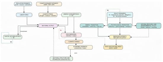
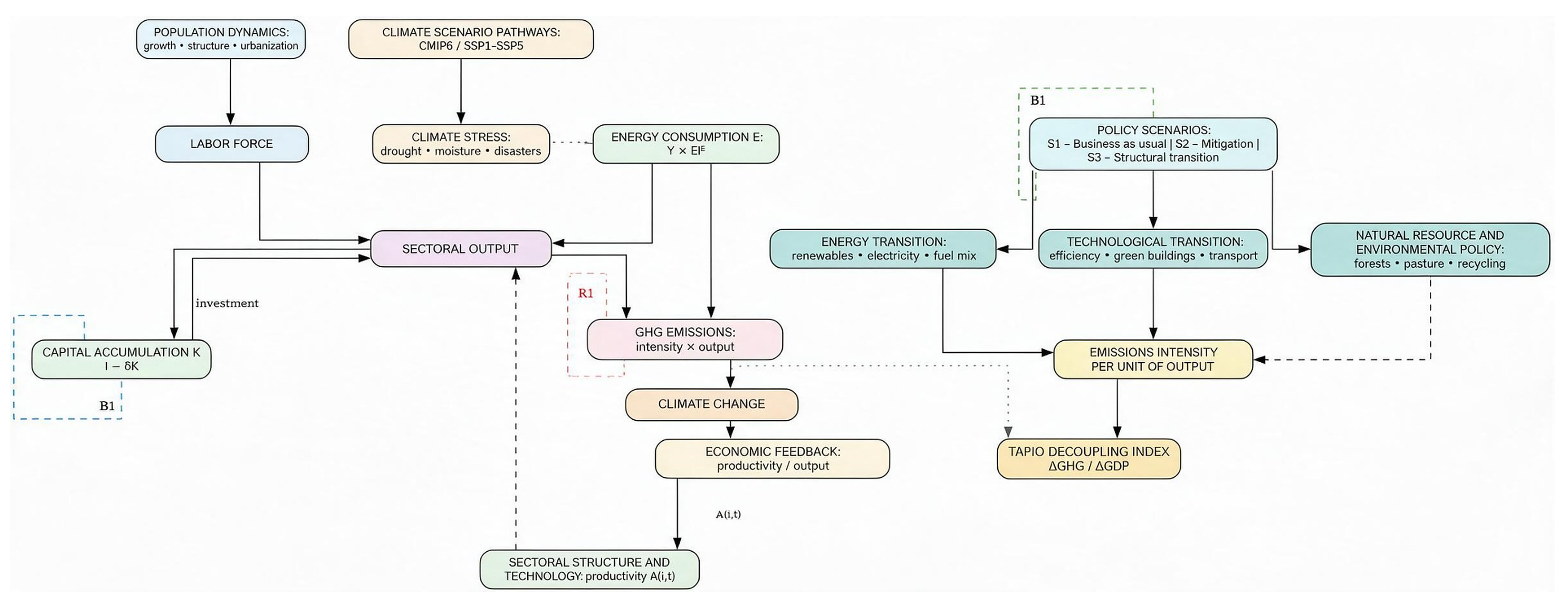
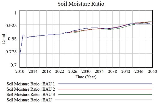
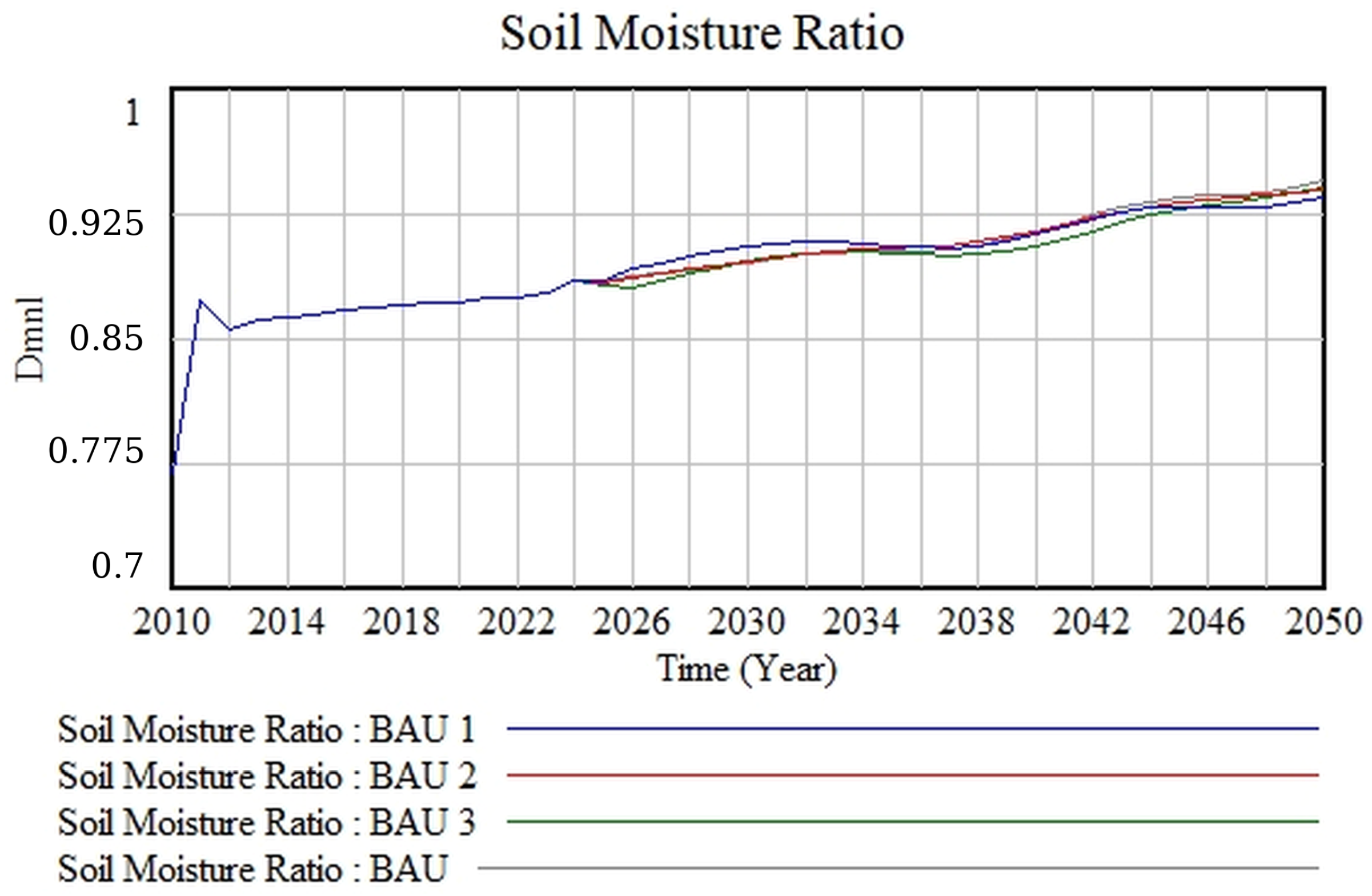
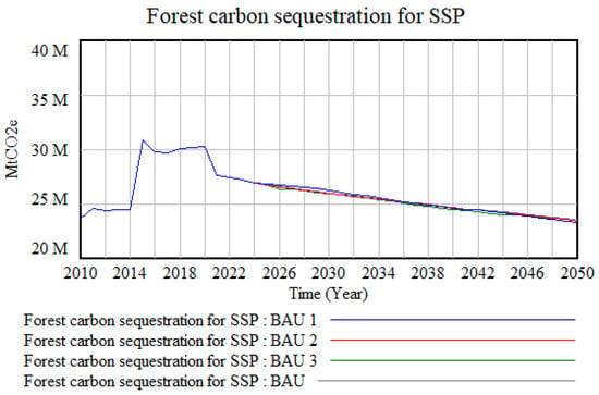
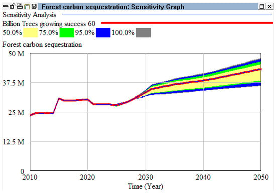
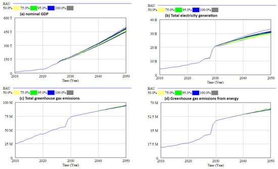
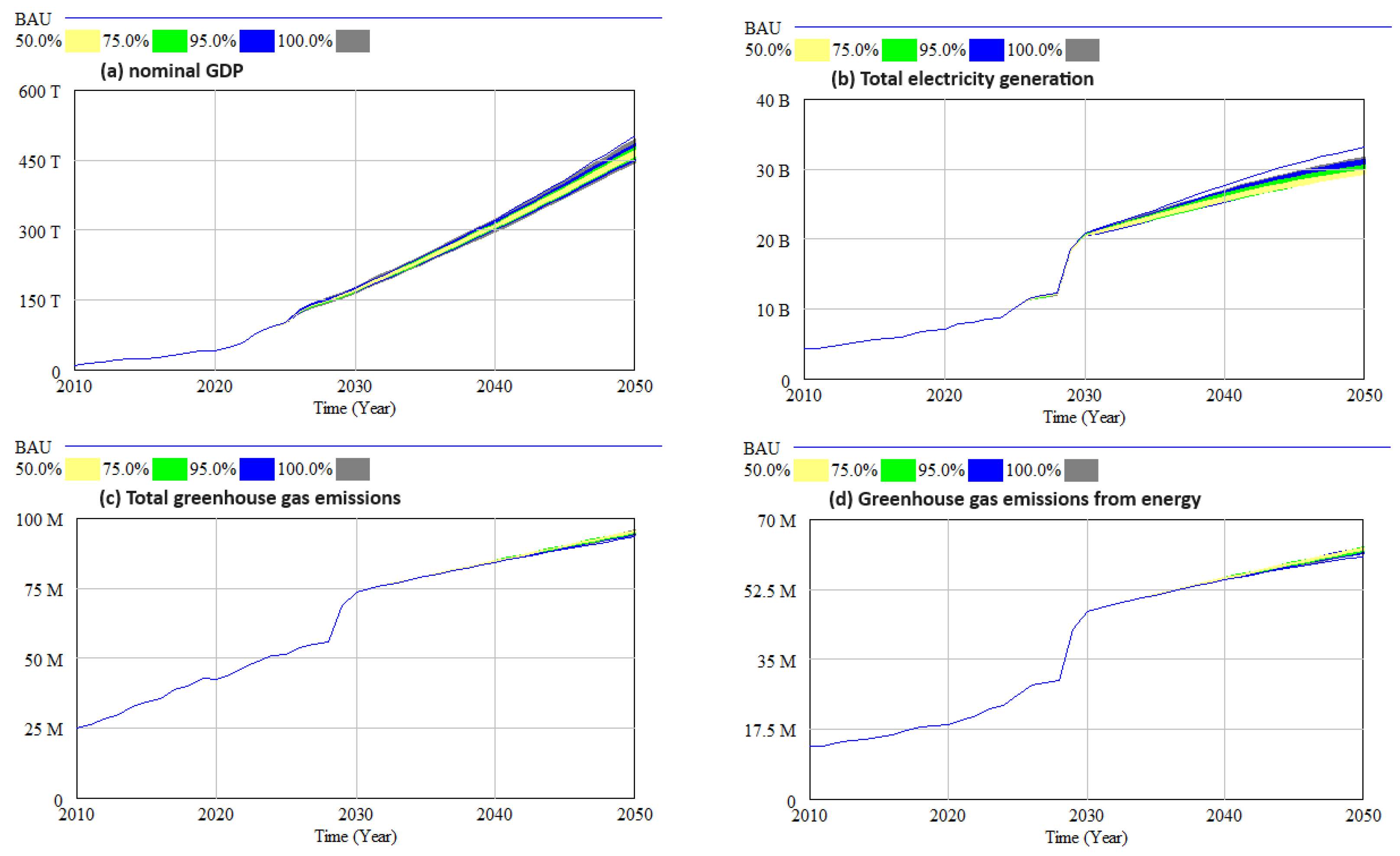
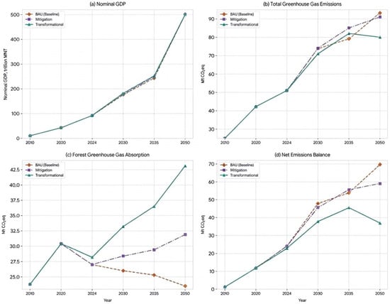
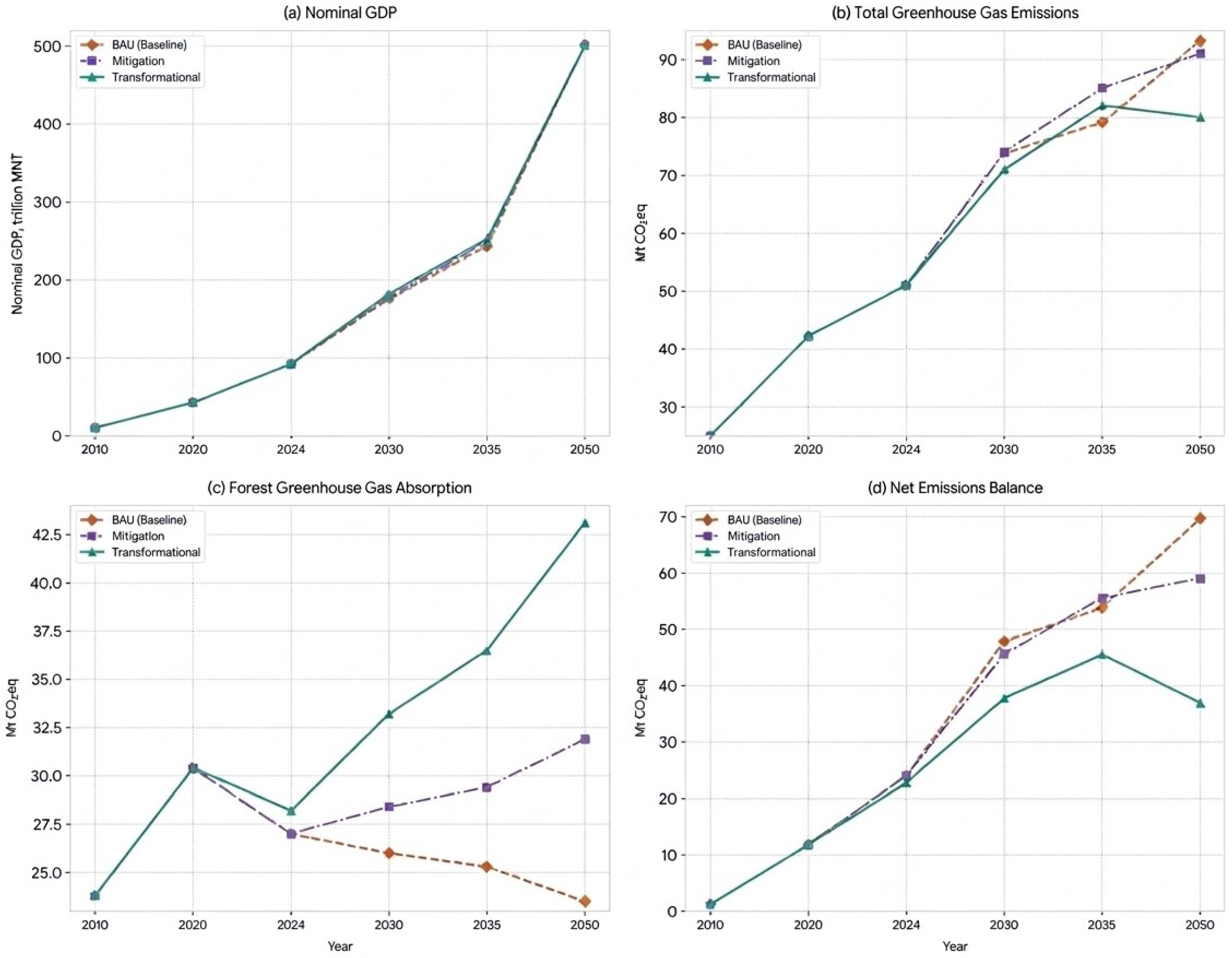
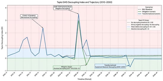
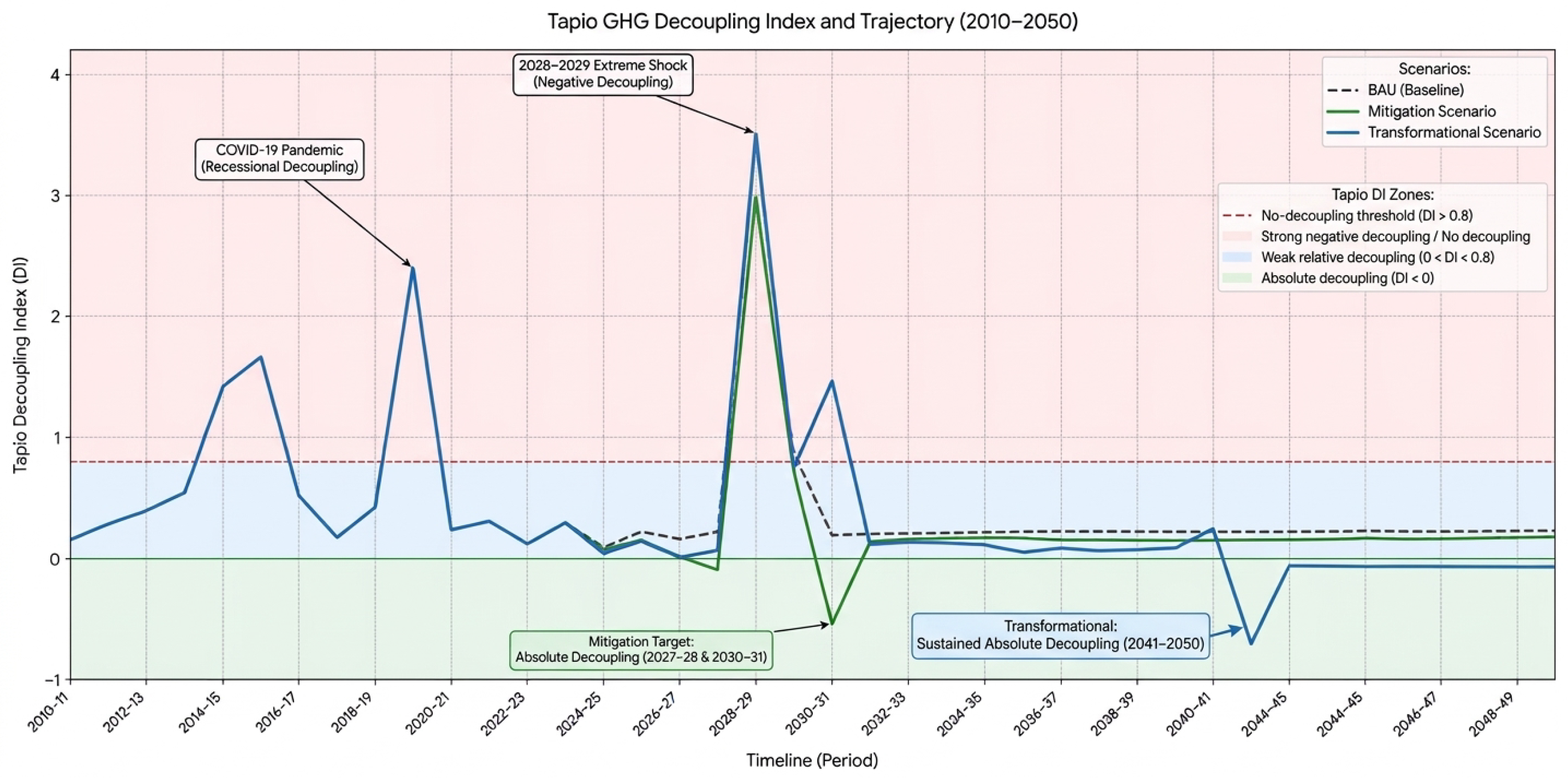

Disclaimer/Publisher’s Note: The statements, opinions and data contained in all publications are solely those of the individual author(s) and contributor(s) and not of MDPI and/or the editor(s). MDPI and/or the editor(s) disclaim responsibility for any injury to people or property resulting from any ideas, methods, instructions or products referred to in the content. |
© 2026 by the authors. Licensee MDPI, Basel, Switzerland. This article is an open access article distributed under the terms and conditions of the Creative Commons Attribution (CC BY) license.