


Abstract
Equity index models usually rely on the index’s own history, which leaves open how far macroeconomic and risk conditions alone can track its level. This study maps five contemporaneous United States predictors, the economic, financial, and political risk indices, the M2 money supply and industrial production, onto the monthly closing level of the Nasdaq-100 index, and interprets the resulting fit with post hoc attribution. The data span 273 months from May 2003 to January 2026, with training to December 2019 and 73 evaluation months, 97.3 per cent of which lie above the largest training level. Fourteen learners are compared in a two-by-two design crossing direct-level and anchored one-month-change targets with static and recursive fitting. Hyperparameters are searched by a tree-structured Parzen estimator and by differential evolution under a matched budget of 60 evaluations. Three attribution methods are then ranked by the stability of the predictor ordering they reproduce, and accuracy differences are tested by a moving-block bootstrap and a Diebold–Mariano statistic. Every learner returns a negative coefficient of determination under the static direct specification, where the mean root mean squared error is 0.9052, against 0.3102 recursively. Extreme gradient boosting, retained at its default configuration because the search worsened it, records an error of 0.1039 and a coefficient of determination of 0.8677, though no test separates it from gradient boosting or extremely randomised trees. Drift (0.0584) and no-change (0.0600) benchmarks, which use index history withheld from the learners, are more accurate than every learner in that configuration. Permutation feature importance is the most stable method at 0.9374, against 0.8289 for Shapley additive explanations and 0.8063 for leave-one-covariate-out, and assigns the money supply 68.28 per cent of importance; placebo and detrending checks show that this reliance reflects the trend the series shares with the index rather than information specific to money, and the ranking is unchanged under grouped and block permutation. An untouched 2015–2019 window and a nested split of the evaluation period confirm these orderings. Retraining cadence and the information set implied by the target formulation therefore outweigh the choice of learner, and because the predictors are contemporaneous, the result describes a concurrent mapping rather than an ex ante forecast.
1. Introduction
Machine learning systems are increasingly asked to predict quantities that will not stay within the range on which those systems were trained. Equity index prediction makes the resulting difficulty concrete and consequential: estimates of a major index feed retirement balances, collateral valuations and corporate investment plans far beyond the firms the index contains, so a learner that quietly ceases to generalise carries that deterioration into every decision taken downstream of it. The period covered by this study spans two systemic dislocations and a sharp monetary tightening, and the index level itself ends far above anything observed in its earlier years. A substantial body of work reports accuracy gains from comparing or combining many specifications, whether for an aggregate index (Xu & Zhang, 2021) or for the cross-section of returns (Hanauer & Kalsbach, 2023), and empirical studies across developed and emerging markets report that risk and uncertainty indicators co-move with equity returns (Chiang, 2019; Korsah & Mensah, 2023). The parallel growth of explainable artificial intelligence (XAI), and of the post hoc attribution methods that dominate it, has encouraged a second use of the same models, in which the fitted predictor is interrogated to establish which inputs carry the most weight (Černevičienė & Kabašinskas, 2024; Weber et al., 2024).
The motivation for the study is practical as well as methodological. Portfolio managers, risk officers and supervisors increasingly rely on machine learning estimates of equity index levels, and on the explanations attached to them, at moments when the market has moved into territory that no historical sample covers; the years after 2020, in which the Nasdaq-100 index more than doubled while monetary and risk conditions changed abruptly, are a clear instance. Three questions then decide whether such a model can be trusted: whether its accuracy survives once the target leaves the training range, whether any reported gain reflects the learner or the way the problem was posed and whether the explanation offered for its predictions is reproducible and valid. Existing studies usually answer these questions separately and seldom on the same fitted model, which leaves users without a joint account of accuracy and explanation under distributional shift. Supplying that joint account, on a deliberately difficult case, is the motivation for this study.
Both uses rest on an assumption that is rarely examined: that the conditions prevailing when a model is estimated continue to hold when it is deployed. Adaptive frameworks developed for load forecasting are designed to counter the deterioration of accuracy that follows once the input distribution moves away from the training distribution (Azeem et al., 2024). Equity index prediction presents the problem in an acute form, because the target itself drifts upward over time and the evaluation period may lie almost entirely outside the numerical range the model has seen. The consequences differ sharply across model families: learners built from local averages cannot return a value beyond the range of their training targets, whereas learners with an unbounded functional form can, though not necessarily in the right direction.
The literature has approached these two concerns largely in isolation. Studies comparing model families for financial series typically report accuracy on chronological splits without examining whether the evaluation targets remain within the range the model was estimated on, so behaviour outside the training support is left unaddressed (He et al., 2023; Song & Choi, 2023). Work on hyperparameter optimisation has established that search strategy materially affects attainable accuracy and has catalogued the available algorithms in depth (Morales-Hernández et al., 2023; Aghaabbasi et al., 2023), yet comparisons between Bayesian and population-based searches under a matched evaluation budget remain uncommon, so reported gains often confound the search strategy with the resources it was granted. The reliability of post hoc attribution has meanwhile come under sustained scrutiny. Controlled evaluations demonstrate that widely used attribution methods can fail to place importance on the features a model is known to rely on (Zhou et al., 2022), and recent critiques question how much confidence Shapley-derived importance rankings can carry when no independent measure corroborates them (Takefuji, 2025a, 2025b). Reviews of model-agnostic explanation in finance identify this fragility as an open problem rather than a settled one (Khan et al., 2025). The common response in applied papers is to present several attribution methods side by side; where they disagree, no criterion for choosing between them is offered. Three gaps follow. First, the contribution of the target formulation and of the retraining protocol to out-of-sample viability has not been separated from the contribution of the model family, so it is unclear whether the choice of learner is the decision that matters when the evaluation window sits outside the training support. Second, Bayesian and metaheuristic searches are seldom compared on identical spaces under identical budgets, and studies rarely state a rule for when a tuned configuration should displace the default one. Third, no accepted procedure exists for resolving disagreement between attribution methods applied to the same fitted model.
This study addresses those gaps on a single, deliberately demanding prediction problem. The general question raised above cannot be settled by a single application, and the study does not claim to settle it; the Nasdaq-100 case is used as a controlled instance in which the difficulty is severe and measurable, so that the design choices governing behaviour outside the training support can be isolated and reported transparently. Section 4.6, Section 4.7 and Section 4.8 repeat the central comparison under alternative chronological splits, on an earlier window untouched, on three further United States equity indices and on a wider predictor set, which indicates how far the conclusions carry beyond this instance. The Nasdaq-100 index is predicted from five monthly macro-risk indicators covering economic, financial and political risk in the United States together with the money supply and industrial production, over a sample split chronologically so that estimation ends in December 2019 and evaluation runs from January 2020 to January 2026. The split is severe by construction: almost the whole evaluation window lies above the largest index level observed during estimation, which turns the exercise into a test of behavior outside the training support rather than a test of interpolation. No lag or transform of the index is supplied to any model, so whatever accuracy is achieved must come from the macro-risk predictors themselves, and any attribution computed afterward refers unambiguously to those predictors. Section 5.2 shows that much of this accuracy reflects the upward trend that the money supply shares with the index, so the predictors are informative chiefly about where the index stands along that trend. The intended application is therefore the contemporaneous estimation of the index level from macro-risk conditions, that is, establishing which level the prevailing macro-risk state is consistent with and which indicators carry that judgement, rather than an operational system for forecasting next month’s index; Section 4.8 reports how accuracy changes when the predictors are restricted to the information actually released at the prediction date.
The investigation proceeds in four stages. A factorial experiment first crosses two target formulations with two retraining protocols across fourteen learners, isolating the design choice that governs whether the problem is tractable at all. Two optimisers, a tree-structured Parzen estimator and a differential evolution metaheuristic, then search identical spaces under an identical evaluation budget, with a single stated rule deciding whether each model proceeds with tuned or default settings. The resulting configurations are compared on training, validation and evaluation data, and differences are subjected to a block bootstrap and a Diebold–Mariano test. Three attribution methods are finally applied to the leading model and assessed not for plausibility but for stability under repeated resampling; the method that reproduces its ranking most consistently is selected, and the interpretation and recommendations are developed on that method alone.
The study is organised around four research questions. RQ1: when the evaluation window lies outside the training support, do the retraining protocol, the target formulation and the information set that the formulation implies matter more for out-of-sample accuracy than the choice of learner? RQ2: under a matched evaluation budget, does a Bayesian optimiser outperform a population-based metaheuristic, and when should a tuned configuration replace the default one? RQ3: which learner leads under the primary configuration, and can its advantage over competing learners, over simpler references using the same information and over history-based benchmarks be separated from sampling noise? RQ4: when attribution methods disagree on the same fitted model, can the reproducibility of their rankings serve as a transparent selection criterion, and does the selected ranking survive separate checks of validity?
The study makes four contributions, each tied to one of these questions. First, it separates the effect of the retraining cadence, the target formulation and the information set from that of the learner within one factorial design and shows that these design factors account for most of the variation in accuracy (RQ1). Second, it compares two optimisers on identical spaces under an identical budget, repeated over independent seeds, and states in advance the rule by which tuned settings are adopted (RQ2). Third, it reports accuracy together with formal tests against competing learners, simpler references and history-based benchmarks, including the unfavourable but informative result that the no-change and drift benchmarks are more accurate than every learner restricted to macro-risk inputs; the value of such a model therefore lies in relating the index to macro-risk conditions and in explaining that relation (RQ3). Fourth, it proposes ranking reproducibility as an explicit criterion for choosing among attribution methods and complements it with grouped, block and placebo permutation checks, so that reproducibility and validity are assessed separately (RQ4). The justification for this design is that each of these choices is usually made implicitly in existing work; making them explicit and testable is what allows the reported accuracy and the reported explanation to be inspected.
Section 2 reviews recent work on index prediction, hyperparameter search and attribution reliability. Section 3 describes the data, the engineered features, the learners, the validation protocol and the attribution machinery. Section 4 reports the factorial experiment, the tuning outcomes and the model comparison, followed by confirmatory evidence from windows not used in the design and checks on other targets, predictor sets and publication lags. Section 5 presents the stability assessment, the resulting predictor ranking and the validity checks of the attribution. Section 6 draws out the practical implications, Section 7 sets out the limitations and Section 8 concludes.
2. Related Work
Comparative and ensemble approaches dominate recent work on index prediction. Xu and Zhang (2021) pooled a large set of autoregressive and vector error-correction specifications for the Chinese stock index under several weighting and trimming strategies and found a shrinkage composite optimal on mean squared error at every horizon examined, which they credited to diversification against mis-specification. He et al. (2023) paired a convolutional recurrent network with an autoregressive moving average component, the first carrying nonlinear structure and the second the linear autocorrelation, and outperformed autoregressive moving average, random-walk and single neural network benchmarks. Song and Choi (2023) contrasted hybrid recurrent architectures on three major indices and reported that the advantage over conventional learners was far more consistent at multi-step than at single-step horizons. Bhambu et al. (2024) built a recurrent ensemble on random vector functional link networks, exploiting the closed-form output layer to keep training inexpensive, and improved on both single networks and several recurrent baselines. Albuquerque et al. (2022) reviewed ensemble methods for financial time-series forecasting, chiefly bagging and boosting, and concluded that combining models usually improves on single models. A limitation shared by these studies is that the index’s own history is the principal input and the evaluation periods largely remain within the range of levels seen during estimation, so the reported gains say little about behaviour once the target leaves the training support; nor do they separate the contribution of the learner from that of the way the target is posed. The present design addresses both points by withholding index history from the learners and by evaluating on a window that lies almost entirely above the training range.
A second strand asks how far nonlinear learners improve on simpler references. Hanauer and Kalsbach (2023) benchmarked tree ensembles and neural networks against linear specifications on a large panel of firm characteristics for emerging market returns; the nonlinear learners performed better out of sample across thirty-two emerging markets. Chu and Qureshi (2023) compared regularised linear models, tree ensembles and neural networks on United States output growth under a recursive design and found no method dominant across horizons, with parsimonious linear models on a few strong predictors competitive at the one-quarter horizon. Yoon (2021) weighed gradient boosting and random forest regression against the official projections of the International Monetary Fund and the Bank of Japan for Japanese real output growth and found both learners more accurate. These studies together indicate that the margin over a well-chosen reference is often narrow and that it depends on the evaluation design as much as on the learner. These findings echo a long-standing difficulty in asset-price prediction: random-walk forecasts have proved hard to improve upon since the evidence on exchange rates (Meese & Rogoff, 1983), and most proposed predictors of the equity premium fail to outperform the historical mean out of sample (Welch & Goyal, 2008); such gains as exist are small and appear only when economically motivated restrictions are imposed (Campbell & Thompson, 2008). What these studies seldom provide is an account of why a reference wins, in particular whether its advantage comes from the information it uses or from the form of the prediction; the factorial design and the information-set decomposition in Section 4.2 are intended to supply that account for the present problem.
Work on hyperparameter search establishes that both the choice of algorithm and the size of the budget matter. Morales-Hernández et al. (2023) separated metaheuristic, metamodel-based and hybrid procedures and catalogued the quality metrics by which such procedures are compared. Aghaabbasi et al. (2023) tuned five classifiers by Bayesian optimisation for a work travel mode choice task and found the gain largest for k-nearest neighbours; Cihan (2025) found on a gasification prediction problem that sensitivity to hyperparameter settings differed markedly across learners, k-nearest neighbours and the elastic net being the least stable. Zhang et al. (2019) used a modified firefly metaheuristic to select the kernel and penalty parameters of a support vector regression model and reduced error relative to support vector regression tuned by other optimisation algorithms, establishing that the parameters of kernel methods warrant a dedicated search. Beniwal et al. (2023) wrapped a genetic algorithm around support vector regression and validated it in a forward-moving design that mirrors deployment, so that the configuration is chosen under conditions that resemble its use. Rizkallah (2025) partitioned regression data by clustering before fitting boosted trees, so that each region receives a model matched to its local structure, and reduced error across forty benchmark data sets. Most of these studies, however, tune with a single optimiser, report the outcome of one search seed and adopt the tuned configuration whenever it improves on the default, however small the margin. Because the validation objective is itself estimated from a limited number of points, small improvements may reflect noise in the objective rather than a better configuration (Cawley & Talbot, 2010). The present study therefore compares two optimisers under a matched budget, repeats both searches over several seeds and states an explicit adoption threshold.
The reliability of post hoc attribution is the least settled of the three strands. Bifarin (2023) demonstrated tree-based Shapley additive explanations on metabolomics classification and showed how such attributions summarise at both the individual and aggregate levels, while cautioning that explanation does not imply causation. Zhou et al. (2022) constructed semi-natural data sets in which the ground-truth attribution is known by design and found that widely adopted methods often failed to concentrate attribution on the features the model was guaranteed to rely on, which led them to caution against treating attribution output as direct evidence of model behaviour. Takefuji (2025a) examined how the sequential error correction of gradient boosting interacts with Shapley-based importance, arguing that emphasis on poorly fitted cases can inflate the weight a model appears to assign and, against the evidentiary standard a regulatory setting imposes, recommended corroborating such rankings with rank-correlation statistics and their significance levels before consequential decisions rest on them (Takefuji, 2025b). Khan et al. (2025) reviewed model-agnostic explanation techniques in finance, called for systematic benchmarking of these methods and flagged the instability of local explanations as an open challenge. Two further issues are rarely addressed in existing work. Permutation-based importance can be distorted when predictors are correlated, because permuting one feature creates combinations of inputs that never occur in the data (Strobl et al., 2008; Hooker et al., 2021), and standard permutation also ignores the serial dependence of time series. In addition, agreement between methods, or the stability of a single method, does not by itself establish that an explanation is correct. These considerations motivate the separate treatment of reproducibility and validity in this research.
Azeem et al. (2024) addressed the deterioration of accuracy under shifting input distributions with a transfer-learning framework that adapts a deployed model as conditions change, designed for load forecasting under concept drift. Taken together, this body of work establishes that ensembles usually help but by narrow margins, that tuning matters yet is rarely compared under matched budgets and that attribution methods disagree without an accepted means of resolution. The present study responds to all three observations within one experimental design. Read critically, the literature offers accurate models but rarely examines behaviour outside the training support, offers tuning gains without controlling the budget or the seed and offers explanations without a criterion for choosing between them or a check of their validity. The present study is positioned at the intersection of these three gaps rather than as a proposal for a new learner.
3. Data and Methods
3.1. Data Set and Notation
The study uses monthly observations spanning May 2003 to January 2026, giving = 273 consecutive months with no missing entries. Let Pt denote the closing level of the Nasdaq-100 index in month t, for t = 1, …, T. Because the index grows multiplicatively and spans a wide numerical range over the sample, every model is trained on the natural logarithm of the level,
where yt is the transformed target in month t, and ln(⋅) is the natural logarithm. Equation (1) places the target on an additive scale, so that a fixed absolute error corresponds to a fixed proportional error of the index at any level.
Five macro-risk series act as predictors: the United States Economic Risk Index (ERI), the United States Financial Risk Index (FRI), the United States Political Risk Index (PRI), the M2 money supply (M2) and the Industrial Production Index (IPI). zj,t denote the raw value of predictor j in month t, with j = 1, …, J and J = 5. The money supply is measured in billions of United States dollars, industrial production is an index number and the three risk indices are bounded rating scales carrying no unit. M2 and IPI, being strictly positive and wide-ranging, enter in logarithms; the risk indices enter unchanged. Denote the resulting transformed predictor by . All series are the latest available vintages retrieved in 2026, so M2 and industrial production include every revision published up to that date; the real-time vintages that a user would have seen at each date (Croushore & Stark, 2001) are not used. The two series are also released with a delay, M2 on the fourth Tuesday of the following month and industrial production about two to three weeks after the end of the reference month, whereas the risk ratings are updated monthly by their provider. The consequences of both points for the intended application are examined in this study.
The sample is divided at a fixed date. Months t = 1, …, T0 with T0 = 200, covering May 2003 to December 2019, form the training window; the remaining T − T0 = 73 months, covering January 2020 to January 2026, form the evaluation window. The division is chronological, so no information dated after December 2019 contributes to any quantity used to fit a model or to choose its configuration.
3.2. Feature Construction
Each predictor contributes its contemporaneous transformed level together with two short-horizon changes, which convey direction and pace of movement as well as position:
where is the feature vector in month t, d = 3J = 15 and h ∈ {1,3} is the change horizon in months. The lags required by Equation (2) are available from May 2003 onwards: zj,t is defined for t = −2, …, T with t = 1 denoting May 2003, so the analysis sample starts at the intended date with no rows discarded. Two properties of Equation (2) matter. Every feature is a function of the five macro-risk predictors alone: neither Pt nor any lag or transform of it appears in xt, so any attribution computed on such a model necessarily refers to a predictor; and each feature belongs to exactly one predictor, so feature-level attributions can be summed within groups without ambiguity. In plain terms, Equation (2) describes each month by where every indicator stands, how much it moved over the last month and how much over the last quarter, so that a learner can distinguish a high but falling reading from a high and rising one.
3.3. Target Formulations
Two ways of posing the learning problem are compared. In the direct formulation, the learner maps the macro-risk state onto the level itself,
where f is a learner with hyperparameters θ, are the parameters it acquires when fitted under those hyperparameters and is the predicted log level. Equation (3) requires the learner to locate the index level from the macro-risk state alone. In the anchored formulation, the learner instead predicts the one-month change, which is added to the level observed in the preceding month,
with g the learner of the change and yt−1 the previously observed log level. The anchor in Equation (4) is applied outside the learner and is not a feature, so the input to g remains exactly the vector of Equation (2). The first formulation must supply the level itself; the second supplies only the increment and receives the level from the anchor. The two formulations therefore differ in two respects at once: the quantity the learner is asked to predict and the information available to the final prediction, since the anchored prediction receives the realised previous level through the anchor, while the direct one does not. To separate the two, Section 4.2 adds an information-matched direct cell, in which the previous log level enters the direct learner as a sixteenth feature and an anchored cell without macro-risk features, which reduces to a recursively estimated drift.
One property of both bounds what the reported accuracy means. The predictor vector xt carries the same month as the target yt, so the mapping is contemporaneous. The evaluation is out of sample chronologically, nothing dated after month t contributes and under Equation (5), the parameters use only months up to t − 1, but it is not an ex ante forecast that could have been issued before month t began, since several predictors are published with a reporting lag. What is measured is the transferability of a contemporaneous macro-risk-to-index mapping across a regime boundary. The exercise is accordingly a same-month mapping. It resembles nowcasting (Bańbura et al., 2013) only in targeting the current period: unlike a nowcast, it does not use the real-time data flow, and its target is observed before the predictors are released. It asks which index level the macro-risk state of a month supports, and its natural uses are contemporaneous valuation checks, scenario analysis and the explanation of index movements, rather than the issue of forecasts. Section 4.8 reports the same configuration with each predictor lagged to the month that would actually have been published when a prediction is made, which converts it into a genuine ex ante forecast.
3.4. Retraining Protocols
Two protocols govern how often a learner is re-estimated over the evaluation window. Under the static protocol, a single fit on months 1, …, T0 is applied unchanged to every evaluation month. Under the recursive protocol, the learner is re-estimated before each prediction on all observations that precede it,
where denotes the parameters estimated from the expanding window that ends in month t − 1, and is the training loss of the learner concerned. The summation limit in Equation (5) makes explicit that no realised target dated t or later contributes to the parameters used for month t, and the protocol begins from exactly the training window specified above. Hyperparameters are held fixed at the values chosen on that window and are not re-optimised as it expands. Equation (5) states the direct case; the anchored case replaces the response ys by the change ys − ys−1, runs the sum from s = 2 and adds yt−1 to the prediction as in Equation (4). Intuitively, Equation (5) describes a model that is re-estimated every month with all data available up to that point, as a user updating the model monthly would do, and that is then asked for a single prediction.
3.5. Learning Algorithms
Fourteen learners spanning penalised linear, kernel, instance-based, tree ensemble, neural and probabilistic families are compared, two of them composite learners introduced in this study. They are as follows: ordinary least squares (OLS), ridge regression (RIDGE), elastic net (ENET), support vector regression (SVR), k-nearest neighbours (KNN), random forest (RF), extremely randomised trees (ET), gradient boosting regression (GBR), extreme gradient boosting (XGB), light gradient boosting machine (LGBM), multilayer perceptron (MLP), Gaussian process regression (GPR), the ridge-boosted hybrid (HYB) and the stacked generalisation ensemble (STACK).
The twelve non-composite learners standardise their features using training-window moments and standardise the target by an invertible transformation that leaves the predicted range unrestricted. The two composite learners scale internally instead, each standardising features within its own constituent parts and fitting directly to the untransformed target, because their combination steps are defined on the target scale.
The penalised linear family, defined by Equation (6), estimates coefficients and intercept b by solving
where is the set of training months, λ ≥ 0 is the penalty strength and ψ ∈ [0,1] is the mixing parameter. Setting ψ = 0 recovers ridge regression, ψ ∈ (0,1) gives the elastic net (Zou & Hastie, 2005) and λ = 0 gives ordinary least squares, so Equation (6) accounts for three of the fourteen learners. The first term of Equation (6) rewards fit to the training data, and the second penalises large coefficients, which stabilises the estimates when predictors are correlated, as the three risk indices are here. Support vector regression, stated in Equation (7), solves the ε-insensitive problem
in which C > 0 is the penalty on deviations, ε ≥ 0 is the width of the insensitive tube, ξt and are slack variables for month t, and ϕ(⋅) is the feature map induced by the radial basis kernel with width parameter γ > 0. Put simply, Equation (7) ignores errors smaller than the tube width and penalises larger ones linearly, so that the fit is governed by the months it reproduces least well. Randomised tree ensembles instead average the outputs of B trees, as in Equation (8),
where τb is the b-th regression tree grown on a resampled or randomised view of the training data. Random forests (Breiman, 2001) and extremely randomised trees (Geurts et al., 2006) differ in how split points and candidate features are drawn and in whether trees are grown on resampled or complete data. Because every term of Equation (8) is an average of training targets, the ensemble cannot return a value outside the range of those targets, a property that becomes decisive in Section 4.2. Gradient boosting (Friedman, 2001) builds an additive expansion instead, given by Equation (9),
in which Fm is the model after m stages, F0 is the constant minimising the loss on the training targets, η ∈ (0,1] is the learning rate, M is the number of stages and τm is fitted to the negative gradient of the loss at stage m. The regularised variant used by extreme gradient boosting (Chen & Guestrin, 2016) augments the stagewise criterion of Equation (9) with a complexity term, giving Equation (10),
where Lm is the number of leaves of the m-th tree, vm collects its leaf weights, γc ≥ 0 penalises additional leaves and λr ≥ 0 shrinks leaf weights. The histogram-based implementation of the same principle, entered here as a separate learner, bins each feature into a histogram before searching for splits, using the implementation of the light gradient boosting machine (Ke et al., 2017). In words, boosting builds the prediction step by step, each new tree correcting the errors left by the previous ones, and the penalty in Equation (10) discourages trees with many leaves or extreme leaf values, which limits overfitting on two hundred monthly observations. The multilayer perceptron composes affine maps with a nonlinearity, as set out in Equation (11),
with and the weights and biases of layer and σ(⋅) the rectified linear activation applied elementwise, H the number of hidden layers and the activation of layer ; the output layer applies a single affine map to h(H). Gaussian process regression returns the posterior mean of Equation (12),
where K is the matrix of kernel evaluations among training inputs, κ* collects the kernel evaluations between xt and the training inputs, is the noise variance, I is the identity matrix and y stacks the training targets. The kernel sums a linear, a squared-exponential and a white-noise component, so that the posterior mean retains a non-constant response beyond the range of the training inputs. Equation (11) passes the inputs through successive layers of weighted sums and rectifications, and Equation (12) predicts each month as a similarity-weighted combination of the training targets, the weights being set by the kernel.
Two composite learners are introduced. The first, the ridge-boosted hybrid of Equation (13), adds a boosted correction to a penalised linear fit,
where G is a gradient-boosting machine fitted to the residuals of the linear term, and ω is a shrinkage weight damping the correction. The linear term supplies an unbounded response that remains defined outside the training support, while the boosted term absorbs curvature within it. The second, a stacked generalisation ensemble in the sense of Wolpert (Wolpert, 1992), combines Q = 3 structurally different base learners through Equation (14),
where is the forecast of base learner q, α0 is an intercept and the weights αq are estimated by a non-negative ridge meta-learner on pooled out-of-fold predictions. The constraint in Equation (14) prevents any member from entering with a negative weight; since the weights need not sum to one, the blend is not a convex combination of its members. Equations (13) and (14) thus combine learners of different kinds, the hybrid by adding a damped nonlinear correction to a linear fit and the ensemble by weighting the forecasts of its members according to how well they predicted out of fold.
3.6. Validation Protocol and Hyperparameter Optimisation
Model selection uses a one-step-ahead rolling-origin scheme confined to the training window, which reproduces the recursive deployment of Equation (5). Let denote a set of validation origins drawn from the later part of the training window. The objective minimised by both optimisers is
where are the parameters obtained by fitting the learner with hyperparameters θ to months 1, …, o − 1, and is the number of origins. Equation (15) never evaluates a month from the evaluation window. Equation (15) therefore measures how well a configuration would have predicted months it had not seen, using the training window alone, which is the quantity that matters when the model is deployed recursively.
Two optimisers search the same space under the same evaluation budget. The tree-structured Parzen estimator (TPE) (Bergstra et al., 2011), as implemented in the Optuna framework (Akiba et al., 2019), models the density of hyperparameter vectors conditional on the observed objective values and proposes the point that maximises the ratio given in Equation (16),
in which is a quantile of the objective values seen so far and the two densities are kernel estimates fitted to the corresponding groups of trials, the ratio being applied only after a startup phase has made both groups non-empty, so Equation (16) directs the search towards regions that have already produced low objective values. Informally, the estimator learns from earlier trials which regions of the search space tend to produce low validation error and samples more often there, whereas differential evolution moves a population of candidates by combining the differences between them, which favours broad exploration. Differential evolution (DE) (Storn & Price, 1997) instead maintains a population of candidate vectors, encoded in this study on the unit cube, and generates a donor by
in which Np is the population size, is the differential weight, r1,r2,r3 are three distinct indices drawn from the population excluding i and returns the donor to the unit cube coordinatewise, D denoting the number of searched hyperparameters. The donor produced by Equation (17) is recombined with the parent coordinatewise, under a crossover probability written CR, according to Equation (18),
in which vc is a uniform draw on [0,1], CR ∈ [0,1] is the crossover probability and c⋆ is a coordinate selected at random so that at least one coordinate is inherited from the donor. The candidate replaces the parent when its objective is not worse. Both optimisers receive the same seed and the same number of objective evaluations, so the comparison is not confounded by the resources granted to them. A single rule decides which configuration is carried forward for every model. The optimised configuration replaces the default only when it lowers by more than one per cent in relative terms; otherwise the default configuration is retained and reported as such. Where the rule adopts tuning, the optimiser with the lower value of Equation (15) supplies the setting. The threshold of one per cent is set to exceed the change in Equation (15) that can arise without any change of configuration: the objective is an average over thirty validation origins, and refitting a default learner that draws random numbers under different seeds moves it by amounts of that order (Section 4.3). Requiring a larger improvement guards against adopting a configuration whose apparent gain is noise in the objective, and the sensitivity of the adoption decisions to the threshold, together with repetitions of both searches under further seeds, is reported in Section 4.3.
3.7. Performance Metrics
Let be the error in month t, and let be the set of months over which a metric is computed, of size . Four metrics are reported. The coefficient of determination, given by Equation (19),
measures the share of variation reproduced relative to the mean of the same set and becomes negative when a model performs worse than that mean, which is why Equation (19) is informative about behaviour outside the training support. The mean absolute error of Equation (20),
reports average deviation in units of yt, while the root mean squared error of Equation (21),
weights larger deviations more heavily and is the quantity minimised during tuning. To express accuracy on the scale of the index rather than its logarithm, forecasts are transformed back and summarised by the mean absolute percentage error of Equation (22),
which is reported in per cent of the observed index level. Taken together, Equation (19) indicates whether a model improves on predicting the average level of the window, Equations (20) and (21) give the typical size of the error in log points, an error of 0.10 corresponding to a misstatement of the index of roughly ten per cent, and Equation (22) expresses the same error directly in per cent of the index level.
3.8. Reference Benchmarks
Two reference forecasts are reported alongside the learners. The no-change benchmark sets , and the drift benchmark adds the average monthly change estimated on the training window. Both draw on the realised history of the index, which Equation (2) withholds from every learner. They are reported separately and excluded from the selection of the leading model; their role is to indicate what a prediction with direct access to the previous level can achieve.
3.9. Attribution Methods
Three model-agnostic attribution methods are applied to the leading model: Shapley additive explanation (SHAP), permutation feature importance (PFI) and leave-one-covariate-out (LOCO), drawn respectively from (Lundberg & Lee, 2017; Lundberg et al., 2020; Fisher et al., 2019; Lei et al., 2018). Because the primary configuration re-estimates the learner before every evaluation month, the object explained is that sequence of monthly fits rather than a single static fit. The Shapley additive explanation (Lundberg & Lee, 2017) of feature k at input x is the weighted average of its marginal contributions over all subsets of the remaining features,
where indexes the features, is a subset of th and is the expected model output when only the features in are fixed at their values in x, and the remainder are drawn from a reference set. Equation (23) is estimated by sampling. Permutation importance (Fisher et al., 2019), given by Equation (24), which extends the permutation scheme introduced for random forests (Breiman, 2001), measures the deterioration in accuracy when a feature is made uninformative,
where denotes the r-th random permutation of feature k across the evaluation months, Bπ is the number of permutation repetitions, and RMSE without an argument is the unperturbed value. Leave-one-covariate-out, defined in Equation (25), removes a whole predictor group and refits,
in which RMSE−j is obtained after deleting every feature belonging to predictor j and repeating the whole recursive sequence of fits on the remaining features. Because Equation (25) already operates at the level of a predictor group, its output requires no further aggregation. In both Equations (24) and (25) a negative value, arising when permuting or deleting a feature happens to lower the error, is set to zero before normalisation: a feature whose removal improves accuracy carries no positive attributable importance. The convention is applied identically to both methods and produces the reported shares. Feature-level scores from Equations (23) and (24) are mapped onto predictors and expressed as shares by Equation (26),
where is the set of feature indices belonging to predictor j, ak is the feature-level score of feature k produced by whichever method is in use, the mean absolute Shapley value of Equation (23) over the evaluation months or the permutation score of Equation (24) and Sj is the resulting percentage share, which sums to one hundred across the five predictors. Because partitions the feature set and contains no target-derived entry, the shares of Equation (26) rank predictors and nothing else. Should a repetition produce a zero total, every share is set to zero, and that repetition contributes no ordering; no repetition here was degenerate. In practical terms, Equation (23) distributes each prediction among the features, Equation (24) asks how much accuracy is lost when the values of a feature are shuffled, and Equation (25) asks how much accuracy is lost when a predictor is removed and the model re-estimated without it; Equation (26) converts all three into percentage shares of the five predictors so that they can be compared on one scale.
3.10. Attribution Stability
Each method is repeated N = 20 times. Every repetition redraws the random seed governing the method and a single mask retaining eighty-five per cent of the months in the sample; each monthly fit then uses the retained months preceding it, so the mask is common across origins and the retained count grows with the expanding window. The Shapley method additionally redraws its reference set at every evaluation month. Let be the N × J matrix whose entry is the rank assigned to predictor j in repetition i, with rank one denoting the largest share. Equal shares receive the average of the ranks they occupy, which matters because leave-one-covariate-out returns exact zeros for predictors whose deletion does not raise error. Stability is summarised by the mean pairwise Spearman correlation.
where corr() is the Pearson correlation of the two mid-rank vectors, which is the tie-aware form of the rank correlation and reduces to the familiar difference formula when no ranks are tied, and by Kendall’s coefficient of concordance
where Tj is the rank sum of predictor j, its average, and is the tie-correction term for repetition i, in which tig is the size of the g-th group of tied ranks in that repetition. Both Equations (27) and (28) approach unity when repetitions agree on the ordering and fall towards zero when they do not. Two further descriptors accompany them: the proportion of repetitions placing the same predictor first and the mean across predictors of the standard deviation of their assigned ranks. The method with the strongest agreement is selected, and the attribution section is developed on it alone. Both statistics answer the same question, namely whether repeating the attribution on slightly different data returns the same ordering of predictors; values close to one indicate a reproducible ordering.
Reproducibility and validity are distinct properties, and Equations (27) and (28) measure only the first: a method can return the same ranking every time and still credit the wrong predictor. Two checks of validity are therefore reported separately in Section 5.4. The first addresses the distortion that correlated predictors cause in Equation (24) (Strobl et al., 2008; Hooker et al., 2021), together with the serial dependence of the time-series inputs, which standard permutation ignores. In grouped permutation, the three features of a predictor are permuted jointly with one common row permutation, so the link between a predictor’s level and its own changes is kept (Au et al., 2022); in grouped block permutation, the evaluation months are additionally cut into consecutive blocks of six, and only the order of the blocks is shuffled, so serial dependence within each block is also kept. The second is a placebo check: two artificial predictor groups with no relation to the index, white noise and a random walk with the drift and volatility of log M2 over the training window are added to the inputs, and each method is asked how much importance it assigns to them. A valid method should give the noise group essentially nothing, and the share given to the trending placebo shows how much credit a predictor can receive simply for trending upwards.
3.11. Comparing Forecast Accuracy
Differences between models are assessed on the loss differential , where eA,t and eB,t are the errors of two competing forecasts in month t. A moving-block bootstrap with block length six and five thousand replications resamples δt while preserving short-range serial dependence, yielding a percentile interval for the mean loss differential. The Diebold–Mariano statistic (Diebold, 2015), introduced by Diebold and Mariano (Diebold & Mariano, 1995),
provides a parametric counterpart, in which is a heteroscedasticity- and autocorrelation-consistent estimate of the long-run variance of the differential δt itself, formed with Bartlett weights over ⌊4(n/100)2/9⌋ lags, and n is the number of evaluation months. Estimating the variance this way allows for serial correlation in the loss differential rather than assuming it away. An interval from the bootstrap that contains zero, or a large p-value attached to Equation (29), indicates that the two predictions cannot be separated on the available evidence. In plain terms, Equation (29) asks whether the average difference in squared errors between two models is large relative to its sampling variability, allowing for the fact that monthly errors are correlated over time.
3.12. Implementation
All experiments were carried out in Python 3.9 using scikit-learn 1.6.1 (Pedregosa et al., 2011), XGBoost 2.1.4, LightGBM 4.6.0, Optuna 4.9.0 and SHAP 0.49.1. The differential evolution optimiser was implemented directly so that every search control is explicit, and a fixed seed governs every stochastic component.
3.13. Framework Overview
Figure 1 brings together the preceding subsections as a single procedure, from the construction of the predictor features through the factorial screen and the matched-budget search to the accuracy comparison and the stability-based choice of attribution method.
Figure 1.
Research framework.
3.14. Separating Exploratory from Confirmatory Evidence
Because the January 2020 to January 2026 window informed the choice of formulation and protocol before it was used to score them (Section 7), two further evaluations are added whose months played no part in any design decision, because evaluation on data that informed model or protocol choices is optimistically biased (Cawley & Talbot, 2010). In the nested split, the leading learner is chosen on January 2020 to December 2022 alone and then scored, together with every competitor, on January 2023 to January 2026, which does not enter the choice. In the earlier confirmatory window, the design fixed after the exploratory phase, direct target, recursive protocol and default configuration of every learner is re-run unchanged with estimation ending in December 2014 and evaluation running from January 2015 to December 2019, months that were never scored by any exploratory diagnostic; default configurations are used so that the tuning origins, which fall in that period, cannot leak into the scores. The pairwise tests of Section 4.5 are also reported with a Holm adjustment for the thirteen comparisons (Holm, 1979). Results obtained on the main evaluation window are described as exploratory in what follows, and results from these two designs as confirmatory.
3.15. Additional Checks
Five further groups of checks are run on the primary configuration, each with the learners at their default settings unless stated. (i) Information set: the cells described in Section 3.3 that hold either the target or the information fixed. (ii) Shared trend and simpler references: a linear time trend, M2 alone, the five predictor levels in a linear regression, a specification in which the index and every predictor level are detrended at each origin using the preceding months only, a fully differenced specification in which the one-month change of the index is predicted from the ten change features alone and placebo runs in which the M2 features are replaced by a simulated random walk or by a time index. (iii) Behaviour over time: a rolling window of the most recent two hundred months in place of the expanding one, alternative split dates and grouped permutation importance computed within each subperiod. (iv) Information available at the prediction date: the predictors lagged by their publication delays. (v) Other targets and predictors: the factorial design of Section 4.2 repeated for the S&P 500, the Dow Jones Industrial Average and the Nasdaq Composite and the primary configuration re-run with four further monthly series added to the predictors.
4. Results
4.1. The Evaluation Window Lies Outside the Training Support
Table 1 sets out the composition of the two windows and makes the difficulty of the experiment explicit. The Nasdaq-100 index (NDX) averages 3247.30 index points during the training window and 15,787.58 during the evaluation window, and 97.3 per cent of evaluation months record a level above the largest value observed during estimation. The predictors do not shift uniformly. The money supply moves entirely beyond its training range, every evaluation month exceeding the training maximum, whereas the economic risk index, the political risk index and industrial production never exceed theirs, and the financial risk index does so in only 4.1 per cent of months. That column measures exceedance of the maximum alone; the risk indices do fall below their training minima, so the contrast is one of direction rather than of containment. Figure 2 traces the index across both windows on a logarithmic axis, Figure 3 shows the five predictors standardised on training moments, and Figure 4 summarises the linear association among the predictors and the target. The consequence is that a learner is asked to produce values it has never been trained to emit. Learners built from local averages of training targets cannot return a value outside their range at all, while learners with an unbounded functional form can, but only by extending a relationship estimated where the money supply was far lower. Section 4.2 quantifies the result.
Table 1.
Composition of the data set and distributional shift between the two windows.
Figure 2.
Nasdaq-100 index level over the full sample on a logarithmic axis.
Figure 3.
The five macro-risk predictors standardised on training-window moments.
Figure 4.
Pearson correlation among the five predictors and the logarithm of the Nasdaq-100 index (NDX) over the full sample.
4.2. Cadence, Information Set and Formulation Govern Viability More than Model Family
Table 2 reports evaluation-window error for every combination of target formulation and retraining protocol using default configurations, so that the design factors are isolated from the effect of tuning. The direction of the formulation effect is the same for all fourteen learners, though the size of the cadence effect depends on which target is in use.
Table 2.
Evaluation-window root mean squared error on the logarithmic index scale for every combination of target formulation and retraining protocol, using default configurations.
Under the direct formulation with a single static fit, the strongest learner reaches an error of 0.5590, and the weakest 1.6219. Since the target is a natural logarithm, deviations of this size correspond to proportional misstatements of the index large enough that the prediction carries no practical information. No model family escapes: the penalised linear models cluster between 0.8019 and 0.8375, the tree ensembles between 0.6753 and 0.8546 and support vector regression and the multilayer perceptron perform worst at 1.6219 and 1.4646, with the nearest-neighbour regressor close behind at 1.4628. That the ordering of families barely matters here is the first substantive finding: a more flexible learner does not address a difficulty arising from the position of the evaluation window rather than from the shape of the function.
Allowing the same learners to be re-estimated as observations arrive changes the picture markedly. Under the direct formulation, the average error across the fourteen learners falls from 0.9052 to 0.3102, and the best entry in the cell improves from 0.5590 to 0.1039, a reduction of more than four fifths; the two minima belong to different learners, the stacked ensemble under the static fit and extreme gradient boosting under recursive re-estimation. The gain concentrates in the tree ensembles, extreme gradient boosting moving from 0.6753 to 0.1039 and gradient boosting from 0.7027 to 0.1128, while ridge regression improves only from 0.8375 to 0.3668. The asymmetry follows from the mechanism at work: recursive re-estimation shrinks the gap between the value to be predicted and the range already seen to a single month, the regime in which a learner whose output stays close to recent targets becomes adequate, strictly so for the averaging ensembles and in practice for the boosted ones, whereas a global linear fit remains destabilised by the collinear and range-bound risk indices however often it is refreshed.
The anchored formulation attains lower error still and does so under either protocol: the strongest learner records 0.0583 with a static fit and 0.0586 with recursive re-estimation, and the average across learners is 0.0788 and 0.0698, respectively. The cadence effect is far weaker here than under the direct target, where the same average moves from 0.9052 to 0.3102, and recursive re-estimation lowers error for only nine of the fourteen anchored learners. Taken at face value, this would settle the matter in favour of the anchored design, but the reference benchmarks in the lower panel of Table 2 show why that conclusion would be premature. The drift benchmark, which carries the previous month forward and adds the average monthly change estimated on the training window, records 0.0584. The best anchored learner therefore improves on a benchmark that uses no predictor whatsoever by 0.0001, and thirteen of the fourteen anchored configurations under the static protocol do not improve on it at all. The accuracy of the anchored formulation is supplied by the anchor rather than by the macro-risk predictors.
The comparison between the two formulations nonetheless changes two things at once, since the anchored prediction also receives the previous level of the index. Table A1 (Appendix A) separates the two effects. Supplying the previous log level to the direct learner as an additional feature, which gives it the same information as the anchored formulation while keeping the level as the target, lowers the mean error from 0.9052 to 0.5629 under the static protocol and from 0.3102 to 0.1775 recursively; changing the target to the one-month change with that information held fixed lowers it further, to 0.0788 and 0.0698. The division between the two effects depends on the learner. For the unbounded linear learners, the information accounts for almost the whole gain: ordinary least squares records 0.0855 with the previous level as a feature against 0.0845 under the anchored formulation. For the tree ensembles, the formulation itself matters: given the previous level as an input, extreme gradient boosting still records 0.6954 under a static fit, against 0.0694 anchored, because a tree ensemble cannot return a level above those it was trained on even when it is told the previous one, whereas predicting a change removes that ceiling. Finally, an anchored prediction that uses no macro-risk feature at all, the drift re-estimated each month, records 0.0585, as accurate as the best anchored learner, so the macro-risk features add nothing measurable once the previous level is known. The finding of this section is therefore stated more precisely: the retraining cadence and the information set dominate the choice of learner, and the target formulation matters in its own right chiefly for learners whose output is bounded by the training range.
This distinction determines the configuration carried into the remainder of the study. The attribution stage requires a model whose predictions originate in the five macro-risk indicators. Under the anchored formulation, almost the whole prediction originates in the previously observed index level, so attributing such a model would characterise a residual increment rather than the index itself. The direct formulation under the recursive protocol is the configuration in which the entire prediction is generated by the predictors while remaining usable, and it is adopted as the primary configuration. Figure 5 displays the four cells on a logarithmic error axis; the anchored results and the two benchmarks are retained throughout as reference points.
Figure 5.
Evaluation-window root mean squared error for each combination of target formulation and retraining protocol, by model, on a logarithmic error axis.
These results complement rather than contradict earlier comparative work. Studies reporting clear gains from more elaborate architectures, such as the hybrid recurrent and convolutional designs of He et al. (2023) and Song and Choi (2023), supplied the series’ own history as input and did not examine whether the evaluation targets left the range seen in estimation; under those conditions, the learner is the main lever. Once the history is withheld and the evaluation window leaves the training support, Table 2 shows that the learner becomes a secondary choice, which is in line with the finding of Chu and Qureshi (2023) that no method dominates across horizons and that parsimonious linear models remain competitive at short ones, and with the long record of simple benchmarks that are hard to beat out of sample, the random walk for exchange rates (Meese & Rogoff, 1983) and the historical mean for the equity premium (Welch & Goyal, 2008). The practical implication is that the retraining cadence and the formulation of the target should be fixed and justified before any comparison of learners is undertaken, because they determine whether a comparison of learners is informative at all.
4.3. Optimiser Comparison and the Configurations Carried Forward
Table 3 sets out the search space and the settings shared by the two optimisers, and Table 4 reports what each achieved. Twelve of the fourteen learners have hyperparameters worth searching; ordinary least squares has none, and the Gaussian process is estimated by marginal likelihood rather than by an external search, so both are entered at their default settings.
Table 3.
Search space and search settings shared by both optimisers.
Table 4.
Validation root mean squared error of the default and optimised configurations, and the configuration carried forward for each model.
Optimisation is worthwhile for most learners and markedly so for a few. The largest improvement belongs to support vector regression, whose validation error falls from 0.3884 to 0.0795, a reduction of 79.52 per cent; the multilayer perceptron improves by 60.75 per cent, and the light gradient boosting machine by 36.49 per cent. In each of these cases, the default configuration sits far from the region of the space that suits a sample of two hundred monthly observations with fifteen collinear features, and the search locates that region within the allotted budget. Figure 6 traces the best value found against the evaluation count for four representative learners; the curves fall steeply at first and then in irregular steps, several improving well into the second half of the budget, so the allotted sixty evaluations are used rather than exhausted early.
Figure 6.
Best validation root mean squared error found so far against the number of objective evaluations, for four representative models under the tree-structured Parzen estimator (TPE) and differential evolution (DE).
Neither optimiser establishes a general advantage. The tree-structured Parzen estimator returns the lower validation error for eight of the twelve searched learners and differential evolution for the remaining four, and where they differ, the margin is usually small: for ridge regression, the two agree at 0.1555, and for extremely randomised trees, they differ by 0.0005. Differential evolution supplies the setting for the two learners with the strongest validation performance, gradient boosting at 0.0490 and the stacked ensemble at 0.0454, but the pattern across the full set does not support a claim that either search strategy dominates the other on this problem under a matched budget.
Applying the adoption rule uniformly produces a mixed outcome, which is the point of stating the rule in advance. Nine learners proceed with optimised settings, and five with their defaults. Ridge regression is optimised to 0.1555 against a default of 0.1557, a gain of 0.11 percent that does not meet the threshold, so the default is retained. More striking are the two cases in which the search degrades validation performance: the random forest moves from 0.0646 to 0.0648, and extreme gradient boosting from 0.0571 to 0.0635, changes of −0.35 and −11.27 percent, respectively, and both accordingly proceed with their defaults. That a search confined to sixty evaluations of a thirty-origin rolling objective can settle on a configuration inferior to the default is a reminder that the objective in Equation (15) is itself estimated from a modest number of validation points, and that a sufficiently flexible search can fit its noise. Figure 7 compares the default and adopted values across the searched learners.
Figure 7.
Validation root mean squared error of the default and of the optimised configuration for each searched model.
Because a single search seed may flatter or penalise either optimiser, both searches were repeated under further independent seeds, three per learner including the original for the seven less expensive searches and two for the five most expensive ones (gradient boosting, the light gradient boosting machine, extremely randomised trees, the random forest and the stacked ensemble), with the learners’ own seeds held fixed so that only the optimisers vary. Table A2 (Appendix A) reports the results. Across all searches, the tree-structured Parzen estimator returns the lower validation error in 20 of 31 cases, and the median coefficient of variation of the best value across seeds is 1.98 percent for it and 4.01 percent for differential evolution, so the conclusion that neither optimiser dominates is not an outcome of the seed. Extreme gradient boosting is the one learner whose decision changes in a consequential way. Under seed 2, differential evolution finds a configuration with a validation error of 0.0530, 7.20 percent below the default, which the rule would adopt. Scored in the primary configuration, that configuration records 0.1107 on the evaluation window against 0.1039 for the default, a difference that cannot be separated from noise (p = 0.2662) and that would leave it level with gradient boosting; the leading group of boosted ensembles is therefore unchanged, whereas which of its members is nominally first depends on the seed, in line with the tests of Section 4.5. Apart from that case, the decision depends on the seed only for extremely randomised trees and the ridge-boosted hybrid, whose gains lie close to the threshold.
The one per cent threshold of Section 3.6 is calibrated against the noise of the objective. Refitting the default random forest and extremely randomised trees under five learner seeds, with no change of hyperparameters, moves Equation (15) by a standard deviation of 0.68 and 1.31 percent and by up to 1.48 and 3.06 percent across seeds, so improvements smaller than about one per cent cannot be distinguished from refitting noise; the multilayer perceptron is far noisier (17.93 percent), but its gain of 60.75 percent is well clear of that level. The adoption decisions are also insensitive to the exact value: thresholds of 0.5, 1 and 2 percent adopt tuning for the same nine learners, a threshold of zero adds only ridge regression, whose gain is 0.11 percent, and a threshold of five percent removes the elastic net and extremely randomised trees, whose gains of 3.87 and 3.54 percent exceed the noise level.
The pattern agrees with earlier reports that the effect of hyperparameter settings differs markedly across learners (Aghaabbasi et al., 2023; Cihan, 2025), and the deterioration of extreme gradient boosting is an instance of the over-fitting of the selection criterion described by Cawley and Talbot (2010). It differs from the common practice of reporting only tuned results: had every learner been carried forward with its optimised setting, the leading learner of Table 5 would have entered the comparison with a configuration that is worse on its own validation objective. For users, the implication is that tuned and default results should both be reported and that the adoption rule should be stated before the search is run.
Table 5.
Training, validation and evaluation performance of every model under the primary configuration.
Settings common to both optimisers. First optimiser: Tree-structured Parzen Estimator as implemented in Optuna, 60 trials. Second optimiser: Differential Evolution, rand/1/bin, population 10, 5 generations, differential weight , crossover probability CR = 0.9, giving 60 objective evaluations and so matching the trial budget of the first optimiser. Stopping criterion: exhaustion of the fixed evaluation budget, with no early termination. Objective: mean one-step-ahead rolling-origin validation root mean squared error of the logarithmic index level, as defined in Equation (15). Validation scheme: rolling origin over the last sixty months of the training window, evaluated at every second month, the learner being refitted on all preceding observations at each origin. Random seed: 42 for both optimisers and for every stochastic learner. No month from the evaluation window enters the search.
4.4. Model Comparison
Table 5 reports training, validation and evaluation performance for every learner under the primary configuration, with the two reference benchmarks listed separately.
The evaluation results divide the fourteen learners into three groups. Five boosted or bagged tree ensembles occupy the first: extreme gradient boosting attains an evaluation root mean squared error of 0.1039 with a coefficient of determination of 0.8677 and a mean absolute percentage error of 8.22, followed by gradient boosting at 0.1107, the light gradient boosting machine at 0.1114, the random forest at 0.1267 and extremely randomised trees at 0.1390. A second group, comprising the stacked ensemble at 0.2465, the Gaussian process at 0.2585 and the ridge-boosted hybrid at 0.2593, retains a positive coefficient of determination but errs by roughly a quarter in logarithmic terms. The third group, containing every penalised linear specification together with support vector regression, the nearest-neighbour regressor and the multilayer perceptron, records negative coefficients of determination between −0.5540 and −2.4192, placing these learners below the mean of the evaluation window itself, a quantity computed after the fact and therefore a reference rather than a prediction a user could have issued. Figure 8 plots the path of the leading learner against the observed index and the no-change benchmark, and Figure 9 the corresponding monthly percentage error.
Figure 8.
Observed Nasdaq-100 index (NDX) over the evaluation window against the recursive prediction of extreme gradient boosting (XGB) and the no-change benchmark.
Figure 9.
Month-by-month percentage prediction error of the leading model over the evaluation window, computed as the predicted minus the observed index level in per cent of the observed level.
Two features of Table 5 qualify how the ranking should be understood. The first is that training performance carries almost no information: five learners reproduce the training targets exactly or nearly so, with coefficients of determination of 1.0000, and among them are both the strongest learner on the evaluation window and the weakest. The stacked ensemble is a special case in the opposite direction, its training error of 0.2346 exceeding its validation error of 0.0454 because its combination weights are calibrated on out-of-fold base predictions rather than on in-sample ones, so its training column is not comparable with the others.
The second and more consequential feature is a divergence between the validation and evaluation orderings. The stacked ensemble records the lowest validation error of any learner at 0.0454, ahead of gradient boosting at 0.0490 and extreme gradient boosting at 0.0571, yet on the evaluation window, it falls to 0.2465, while extreme gradient boosting leads at 0.1039. The learner that the validation protocol selects is therefore not the learner that performs best where it matters. Since the validation origins all lie inside the training window and inherit its distributional characteristics, while the evaluation window does not, agreement between the two orderings was never guaranteed. This is a substantive finding about validation under distributional shift, and it is the reason the leading learner is identified from the tabulated evaluation results with the validation ordering reported alongside, so that the divergence remains visible.
The leading position of the boosted and bagged tree ensembles is consistent with the evidence surveyed by Albuquerque et al. (2022) and with the comparison of Yoon (2021), in which tree ensembles outperformed official projections of output growth, while the instability of the ordering between validation and evaluation underlines the case made by Beniwal et al. (2023) for a forward-moving validation design that mirrors deployment. What the present results add is the reason: the recursive ensembles succeed because each refit narrows the gap between the month to be predicted and the range already seen, whereas the penalised linear and kernel learners extrapolate a relationship estimated where the money supply was far lower. The implication for model selection is that validation evidence drawn from a stable period should not be taken as evidence about a shifted one.
4.5. Statistical Separation of the Accuracy Differences
Table 6 compares every model with the leading learner using a moving-block bootstrap and a Diebold–Mariano statistic computed from Equation (29), the latter with a long-run variance at the automatic bandwidth, which for this window selects three lags.
Table 6.
Comparison of every model against the leading model.
Gradient boosting cannot be separated from extreme gradient boosting on either instrument: the difference in root mean squared error is 0.0068, the bootstrap interval spans zero at [−0.0012, 0.0038] and the p-value is 0.2726. The light gradient boosting machine and the random forest are separated on both, at 0.0172 and 0.0008, as are the stacked ensemble at 0.0002, support vector regression at 0.0146 and the nearest-neighbour regressor at 0.0101. Extremely randomised trees are separated on neither, with an interval of [−0.0001, 0.0208] that just includes zero and a p-value of 0.1268.
For six further learners, the two instruments disagree, and the disagreement is informative rather than incidental. The Gaussian process, the ridge-boosted hybrid, the multilayer perceptron and the three penalised linear specifications all show bootstrap intervals that exclude zero, ridge regression for instance at [0.0325, 0.2703], while their p-values, between 0.0664 and 0.2031, do not reach conventional levels. Their loss differentials are large and highly dispersed, which widens the parametric standard error faster than it moves the mean, so the bootstrap, which makes no normality assumption, is the more informative of the two here. The supportable statement is that the boosted ensembles occupy the top of the ranking and the penalised linear, kernel and instance-based learners the bottom.
The benchmarks require the opposite conclusion, stated plainly. The drift benchmark records an evaluation root mean squared error of 0.0584 and the no-change benchmark 0.0600, against 0.1039 for the leading learner, and both differences are separated from zero on both instruments, with p-values of 0.0018 and 0.0020. A prediction that carries the previous month forward is therefore more accurate over this window than any of the fourteen learners in the primary configuration, though Table 2 shows the stacked ensemble reaching 0.0583 under a static anchored fit, marginally below the drift benchmark. The two are not competing on equal terms: the benchmarks are supplied with the realised index level one month earlier, which Equation (2) withholds from every learner by design. The restriction applies to the feature vector alone, since under the recursive protocol the learner is refitted on realised targets up to the preceding month, so index history informs its parameters, though no lag of the index is ever an input it can score. Table 6 therefore quantifies the cost of denying the model direct access to the previous level as a predictor, which raises root mean squared error by 0.0455 relative to the drift benchmark and by 0.0438 relative to the no-change benchmark; on the index scale, Table 5 puts the same comparison at 8.22 percent against 4.68 percent. This result places the study within the literature on out-of-sample asset-price prediction, in which simple history-based benchmarks are rarely beaten (Meese & Rogoff, 1983; Welch & Goyal, 2008) and gains over them, where they exist, are small (Campbell & Thompson, 2008), and it limits the practical forecasting value of the macro-risk model: a user who observes the previous month’s index has no reason to prefer the learner for predicting the next level. Its value lies instead in what the benchmark cannot provide, an estimate of the level that the macro-risk state alone supports and an account of which indicators carry that estimate, and it is in that role that the remainder of the study evaluates it.
A related question is whether the complexity of the leading learner is needed at all on the macro-risk information set. Table A3 (Appendix A) compares it with simpler references that receive the same inputs and no index history. A linear time trend records 0.2676, a linear regression on the money supply alone 0.2382 and a linear regression on the five predictor levels 0.2779, all re-estimated each month and all separated from extreme gradient boosting on both instruments, so a simple linear mapping of the same information does not reproduce its accuracy. The advantage lies in the flexible, recursively refitted tree structure rather than in the breadth of the inputs: extreme gradient boosting fitted to the three money-supply features alone records 0.0966, which cannot be separated from the full model (p = 0.4739). Section 5.2 returns to what this implies for the role of the money supply.
4.6. Robustness
Table 7 collects four checks on the leading configuration. Replacing recursive re-estimation with a single static fit confirms Section 4.2 on the tuned configurations rather than the default ones: all five leading ensembles fall to negative coefficients of determination, the best recording 0.6555 against 0.1039. Retraining cadence, not model capacity, is what makes this problem tractable.
Table 7.
Robustness of the leading configuration.
The ablation block is the most informative. Removing the economic risk index, the political risk index or industrial production leaves evaluation error essentially unchanged, at 0.1039, 0.1030 and 0.1016 against 0.1039 with all five predictors, the latter two marginally improving it, while removing the financial risk index raises it slightly to 0.1063. Removing the money supply raises error to 0.4799 and drives the coefficient of determination from 0.8677 to −1.8255. One predictor is thus responsible for almost the whole of the model’s usable accuracy, and the other four are close to interchangeable with their own absence. This block is the raw-error presentation of the leave-one-covariate-out measurement discussed in Section 5, not an independent check of it.
Accuracy is not uniform across the evaluation window. The leading learner records 0.1016 over 2020–2021 and 0.0760 over 2022–2023, but 0.1266 over 2024–2026, where the coefficient of determination turns slightly negative at −0.0711. Figure 8 shows the prediction tracking the index closely through the first two subperiods and lagging it during the later advance, a pattern also visible in Figure 9. Repeating the whole recursive evaluation under five random seeds leaves the error unchanged at 0.1039 with a spread of 0.0000, an outcome that is expected rather than informative: the leading configuration draws no random subsample of rows or features, so it is deterministic given the data, and the check records that determinism rather than measuring sensitivity.
The deterioration in 2024–2026 deserves closer examination, because it is the part of the window furthest from the training data. Table A4 (Appendix A) shows its source. Over 2020–2021, the index rose by 0.625 log points, while the money supply rose by 0.337; over 2024–2026, the index rose by 0.418 log points, but the money supply by only 0.076. Because the leading learner uses the money supply chiefly to locate each month along the upward path of the index (Section 5.2), a period in which the index advances while the money supply barely moves is the one in which that coordinate is least informative, and the predictions lag the advance, as Figure 8 shows. The coefficient of determination also falls for a mechanical reason: within a subperiod of twenty-five months, the variation of the target around its own mean is small, so a moderate error already yields a value near zero. The reliance on the money supply does change over time. Grouped permutation importance computed within each subperiod assigns it 68.03, 31.24 and 58.49 percent, and the economic risk index rises to 56.75 percent in 2022–2023, the period of monetary tightening in which the money supply contracted. Replacing the expanding estimation window by a rolling window of the most recent two hundred months leaves the error essentially unchanged (0.1043 against 0.1039), so the deterioration is not caused by old observations dominating the fit. Table A5 also repeats the primary configuration with estimation ending in December 2015, 2017 and 2021: extreme gradient boosting leads the five ensembles at the first two dates (0.0894 and 0.0964) and is narrowly behind extremely randomised trees at the last (0.1049 against 0.1024), and at every date the drift benchmark remains more accurate (0.0527 to 0.0585). Since the five-seed check of Table 7 only records that the configuration is deterministic, these split and window experiments are the relevant evidence of sensitivity.
4.7. Confirmatory Evidence
The results of Section 4.2, Section 4.3, Section 4.4, Section 4.5 and Section 4.6 were obtained on a window that also informed the design, and they are therefore exploratory. The two designs of Section 3.14 provide confirmatory evidence. In the nested split, reported in Table A6, the learner with the lowest error over January 2020 to December 2022 is extreme gradient boosting (0.0913), and over the subsequent thirty-seven months, which play no part in that choice, it again records the lowest error of the fourteen learners, 0.1148 with a coefficient of determination of 0.7084. As on the full window, its advantage over extremely randomised trees (0.1167, p = 0.7917) and gradient boosting (0.1249, p = 0.2834) cannot be separated from noise, and the drift and no-change benchmarks remain more accurate, at 0.0447 and 0.0485 with p-values of 0.0021 and 0.0030.
The earlier confirmatory window is the stronger test, because none of its months was scored during the exploratory phase. The frozen design was re-run on it without change, and 90 per cent of its evaluation months again lie above the training maximum. Table A7 reproduces every qualitative finding of Section 4. The mean error across the fourteen learners falls from 0.4729 under the static direct cell to 0.1424 under recursive re-estimation; the anchored cells record 0.0473 and 0.0502, the best anchored learner (0.0432) doing no better than the drift benchmark (0.0432); and under the primary configuration, extreme gradient boosting records 0.0595, level with gradient boosting (0.0595, p = 0.9973) and ahead of the stacked ensemble (0.0657) and the random forest (0.0668), while the penalised linear learners do not fall below 0.1583. The drift benchmark is again more accurate than every learner in the primary configuration (p < 0.0001 against extreme gradient boosting).
Two adjustments complete the confirmatory picture. With a Holm correction for the thirteen comparisons of Table 6 (Holm, 1979), reported in Table A8, only the stacked ensemble and the random forest remain separated from the leading learner at the five per cent level (adjusted p-values of 0.0027 and 0.0095), so the other separations reported in Section 4.5 should be read as exploratory. The findings that survive both confirmatory designs are the dominance of retraining cadence over the learner, the leading but not uniquely leading position of extreme gradient boosting among the boosted ensembles, and the superiority of the history-based benchmarks.
4.8. Information at the Prediction Date, Other Targets and a Wider Predictor Set
Table A9 re-runs the primary configuration with the predictors restricted to what would have been published when a prediction is made. In an end-of-month nowcast, the risk ratings of month t are available, but M2 and industrial production are only available for month t − 1; in a start-of-month forecast, issued before month t begins, the risk ratings refer to t − 1 and the two macroeconomic series to t − 2. Extreme gradient boosting records 0.1066 with contemporaneous predictors, 0.1285 as a nowcast and 0.1316 as an ex-ante forecast, with coefficients of determination of 0.8605, 0.7974 and 0.7875, and the other two boosted ensembles deteriorate in the same way. Respecting publication lags therefore raises the error of the leading learner by 21 and 23 percent for the two variants without changing the ordering of the learners, and the drift benchmark is more accurate than every variant (p ≤ 0.0013). The contemporaneous design should accordingly be read as an upper bound on what the macro-risk inputs can deliver at the time a prediction is needed; data revisions, which the latest vintages used here incorporate, could widen the gap further.
Table A10 repeats the design of Table 2 for three further United States equity indices with the same five predictors. The pattern of Section 4.2 recurs for every index: the mean error of the direct formulation falls from between 0.4029 and 0.7485 under a static fit to between 0.1055 and 0.1860 under recursive re-estimation, the anchored cells lie within 0.0169 of the drift benchmark and the drift benchmark remains more accurate than every learner in the direct recursive cell, in which extreme gradient boosting is the most accurate of the four learners for every index. The formulation and cadence findings are therefore not specific to the Nasdaq-100. Widening the information set (Table A11) improves accuracy without altering these conclusions: adding the effective federal funds rate, consumer prices, the oil price and the US dollar index to the five predictors lowers the error of extreme gradient boosting from 0.1039 to 0.0837, of gradient boosting from 0.1132 to 0.0933 and of the light gradient boosting machine from 0.1600 to 0.1325, all still above the drift benchmark (0.0584). Grouped permutation importance on the nine-predictor model ranks the money supply first (39.57 percent) followed by the consumer price index (31.97 percent), so the reliance is now shared between two series that both trend upwards, which agrees with the interpretation of the money-supply share given in Section 5.2.
5. Predictor Attribution
The learner carried into this stage is extreme gradient boosting, which Table 5 places first on the evaluation window on all four reported metrics and which proceeds with its default configuration because the search described in Section 4.3 did not improve on it. Because the primary configuration re-estimates that learner before every evaluation month, the object explained here is the same sequence of monthly fits rather than a single static fit: each month is attributed using the model that produced its prediction and the monthly results are averaged. Because Equation (2) admits only the five macro-risk predictors and their short-horizon changes, every quantity reported below refers to a predictor; no lag or transform of the index enters the model and none can therefore enter a ranking.
5.1. Selecting an Attribution Method by Stability
Table 8 reports the stability of the three attribution methods across twenty repetitions in which the random seed and an eighty-five per cent subsample of the observations available to each monthly fit are redrawn, together with the reference set for the Shapley method. Equal shares are carried as mid-ranks, and the concordance coefficient is tie-corrected, which matters because leave-one-covariate-out returns exact zeros for predictors whose deletion does not raise error. Permutation feature importance reproduces its ordering most consistently, with a mean pairwise Spearman correlation of 0.9374, a coefficient of concordance of 0.9405 and a mean rank standard deviation of 0.2872. Shapley additive explanation follows at 0.8289 and 0.8375 with a dispersion of 0.4330, and leave-one-covariate-out is least stable at 0.8063 and 0.8066 with a dispersion of 0.4623. All three identify the same leading predictor in every repetition, so the separation arises entirely at the lower positions; the criterion therefore ranks reproducibility of the ordering, not of the share magnitudes. Reproducibility is a necessary property of a usable ranking but not a sufficient one, and the validity of the selected ranking is examined separately in Section 5.4.
Table 8.
Stability of each attribution method.
Permutation feature importance is therefore selected, and the remainder of this section and the whole of Section 6 are developed on it alone. The basis for the choice is the stability evidence in Table 8 rather than any judgement about which ranking appears more reasonable, and the criterion does not select the most widely used of the three: the Shapley method places second, and leave-one-covariate-out, whose deletion logic is the most direct, is the least reproducible here. Figure 10 displays the distribution of assigned ranks across repetitions for each method and each predictor, and the tighter boxes of the selected method are apparent in the ordering.
Figure 10.
Distribution of the rank assigned to each predictor across twenty repetitions, by attribution method.
5.2. The Resulting Ranking
Table 9 presents the predictor attribution obtained from the selected method. The money supply accounts for 68.28 percent of total attributed importance and is placed first in every one of the twenty repetitions, giving it a mean rank of 1.00 with a standard deviation of 0.00. The economic risk index follows at 17.31 percent and the financial risk index at 10.38 percent, with mean ranks of 2.05 and 2.95 and a dispersion of 0.22 in both cases, so the second and third positions are themselves close to settled. This holds within the selected method; Section 5.4 shows that the second position of the economic risk index is also robust across permutation schemes, whereas the third position is not robust across methods. The political risk index and industrial production share the remaining 4.03 percent, at 2.40 and 1.63 percent, and their identical mean rank of 4.50 with a dispersion of 0.50 shows that the ordering between those two is not resolved.
Table 9.
Predictor attribution obtained from the selected method on the leading model.
The reason the money supply leads follows from the experimental record rather than from any prior expectation. The primary configuration requires the learner to place the index at a level using contemporaneous macro-risk conditions alone, and Table 1 shows that the money supply is the sole series whose evaluation-window values lie entirely above its training range, matching the behaviour of the target, whose evaluation values exceed the training maximum in 97.3 percent of months. The risk indices barely exceed their training maxima, the financial index doing so in only 4.1 percent of months, so they carry little information about where in an ascending sequence a month falls. What the selected method adds to that account is that the reliance is not exclusive: the two risk indices ranked second and third together receive 27.69 percent, a substantial minority of the total rather than a rounding residue.
The strength of this association invites the question raised by nonstationarity (Granger & Newbold, 1974). Both the index and the money supply trend upwards over the sample; their correlation is 0.9772 in log levels but 0.0692 in monthly log changes and 0.3289 once a linear trend is removed from each. Table A3 reports the corresponding checks. Neither a deterministic trend (0.2676) nor a linear relation with the money supply (0.2382) reproduces the accuracy of the leading learner. However, replacing the three money-supply features with a time index (0.0975) or with a simulated random walk carrying the drift and volatility of log M2 (mean 0.1008 over twenty draws, range 0.0956 to 0.1090) leaves accuracy essentially unchanged, whereas detrending the target and the predictor levels at each origin raises the error to 0.1596. In the fully differenced specification, the predicted one-month changes are unrelated to the realised ones, with a correlation of 0.0078 and an out-of-sample coefficient of determination of −0.3935 against the historical mean change. These results qualify the interpretation of Table 9. Under recursive re-estimation the leading learner uses the money supply chiefly as a smooth upward-trending coordinate that places each month relative to the recent past, and any series with that property serves equally well. The 68.28 percent share is therefore best read as the model’s reliance on the trend information carried by the money supply, not as evidence of a monetary channel that is specific to M2, and the macro-risk inputs carry no measurable information about month-to-month changes of the index beyond the drift. The same reading explains why removing the money supply is so costly in Table 7: it is the only input whose trend matches that of the index.
The ablation block of Table 7 shows the same deletion experiment in raw error units. It is not an independent corroboration of the selected method, since deleting a predictor group and repeating the recursive fits is precisely the leave-one-covariate-out operation of Equation (25), so the two are presentations of one measurement. Removing the money supply raises evaluation error from 0.1039 to 0.4799 and turns the coefficient of determination from 0.8677 to −1.8255, whereas removing the economic risk index leaves error at 0.1039, removing the political risk index lowers it to 0.1030, and removing industrial production lowers it to 0.1016. Deletion and permutation agree on which predictor matters most and disagree on how concentrated that reliance is. The difference is mechanical: deletion permits refitting without the predictor, so the monthly models can partly compensate through the remaining features, whereas permutation disturbs an input at prediction time and leaves the fitted models no opportunity to adjust. Earlier studies relate risk and uncertainty measures to equity returns across developed and emerging markets (Chiang, 2019; Korsah & Mensah, 2023). In the present data, the three risk ratings play a secondary role, and their contemporaneous changes carry little information about monthly index changes, as shown above. The difference is more likely to reflect the measures used, rating scales that move in coarse discrete steps and the level target than to contradict that evidence; a return target with continuously measured uncertainty indices would be the natural setting in which to reconcile the two.
5.3. Consistency Check
Table 10 reports the shares and implied ranks produced by the two methods that were not selected. All three agree decisively on first place: the money supply receives 68.28 percent under the selected method, 93.31 percent under the Shapley method and 99.34 percent under leave-one-covariate-out and is ranked first by each. Beyond first place, the methods diverge. The selected method places the economic risk index second at 17.31 percent, whereas leave-one-covariate-out places the financial risk index second at 0.65 percent, and the Shapley method places industrial production second at 2.01 percent. Under leave-one-covariate-out, the political risk index and industrial production both receive 0.00 percent and therefore share the rank of 4.5. The two methods not selected also concentrate far more weight on the leading predictor than the selected one does. Figure 11 places the three sets of shares side by side. This disagreement below first place is consistent with the evidence of Zhou et al. (2022) that widely used attribution methods can misplace importance, and with the observation of Takefuji (2025a) that boosted models tend to favour one of several correlated features; Khan et al. (2025) call for systematic benchmarking of such methods. The stability criterion does not remove the disagreement, but it makes the choice between the accounts explicit, and Section 5.4 tests whether the selected account is also valid.
Table 10.
Consistency check.
Figure 11.
Share of total attributed importance assigned to each predictor by each of the three attribution methods.
5.4. Validity of the Selected Attribution
Stability establishes that the ranking of Table 9 is reproducible; Table A12 and Table A13 (Appendix A) ask whether it is valid, using the two checks of Section 3.10. When the three features of each predictor are permuted jointly, or jointly in blocks of six consecutive months, the ordering is unchanged and as reproducible as under Equation (24), with mean pairwise Spearman correlations of 0.9379 and 0.9368 against 0.9374. The money supply receives 65.82 and 67.20 percent, the economic risk index 17.89 and 18.25 percent and the financial risk index 11.99 and 10.41 percent, close to the shares of Table 9. Neither the correlation between a predictor’s level and its own changes nor the serial dependence of the evaluation months therefore drives the selected ranking.
The placebo check is more demanding. Every method assigns the white-noise group no importance (0.00 percent under each of them), so none of them manufactures importance for an irrelevant input. The random-walk placebo, by contrast, receives between 39.57 and 50.50 percent, about as much as the money supply itself, whose share falls to between 38.97 and 42.48 percent when the placebo is present. The methods correctly detect that the model relies on trending information, but they cannot distinguish the money supply from any other series that trends in the same way, which agrees with the placebo results of Section 5.2. The secondary positions differ in robustness. The economic risk index keeps between 14.72 and 14.75 percent under every permutation scheme even with the placebos present, so its second place is supported throughout, whereas the share of the financial risk index falls to between 1.53 and 2.14 percent and leave-one-covariate-out ranks it second in Table 10. The ranking below the economic risk index is therefore not robust to the choice of method or input set and should be interpreted with caution.
6. Practical Implications
The recommendations below follow from the attribution reported in Table 9 and from the experimental record that supports it. They are addressed to the design and governance of prediction systems rather than to the conduct of monetary or fiscal policy, which lies outside what this evidence can speak to.
Weight monitoring towards the predictor the model relies on, without treating the rest as inert. Under the selected attribution method, the money supply accounts for 68.28 percent of attributed importance, and the ablation in Table 7 shows that its removal raises evaluation error from 0.1039 to 0.4799. Data governance should be proportionate to that concentration. The selected method nonetheless assigns 17.31 and 10.38 percent to the economic and financial risk indices, respectively, so tracking the money supply alone would discard 31.72 percent of the model’s measured reliance. Section 5.2 adds a qualification: the money supply is relied on mainly for the trend it shares with the index, so its monitoring guards the model’s sense of position rather than a monetary signal, and a structural change in that trend would affect the model more than an ordinary monetary surprise.
Treat the concentration as a property of the task as posed. Table 1 offers an account consistent with the ranking: the money supply is the only predictor whose evaluation-window values lie wholly outside its training range, matching the target, whose values exceed the training maximum in 97.3 percent of evaluation months. The present design does not vary range alignment independently of predictor identity, so this is an interpretation the evidence permits rather than a mechanism it isolates. A formulation with a stationary target would give the risk indices a different opportunity, and the shares reported here should not be carried into such a setting without re-estimation. The placebo experiments of Section 5.2 and Section 5.4 now support this interpretation directly: a time index or a simulated random walk with the drift of M2 can take the place of the money supply without loss of accuracy, and a trending placebo added alongside it receives about as much importance, so the concentration reflects the trend that the leading predictor shares with the target.
Specify the retraining cadence as part of the model. Table 2 and the static block of Table 7 show that the same learners move between usable and unusable depending only on how often they are re-estimated: the leading learner records 0.1039 under recursive re-estimation and 0.6753 under a single static fit, the best static result among the five ensembles being 0.6555. Cadence deserves to be documented, version-controlled, and monitored with the same seriousness as the choice of algorithm, since in this study it mattered considerably more.
Attribute the method that is actually deployed. Because cadence is part of the model, the object an attribution method explains must be the sequence of fits the prediction comes from rather than a convenient single fit. The two are not interchangeable here: Table 2 records 0.1039 for the recursive configuration against 0.6753 for a static fit of the same learner, so an attribution computed on the latter would describe a predictor that was never deployed.
Report a benchmark that uses the target’s own history. Table 6 shows the drift benchmark achieving 0.0584 against 0.1039 for the leading learner, a difference separated from zero at p = 0.0018. A study reporting only the learners would convey an impression of adequacy the benchmark removes. Where a system is restricted to exogenous inputs, the accuracy forgone should be quantified and disclosed.
Use the macro-risk model as an explanatory and monitoring instrument rather than as a forecaster. The evidence of Table 5 and Table 6 and of Section 4.8 is consistent: with the previous level available, a no-change or drift prediction is more accurate, and once the predictors are lagged to their release dates, the macro-risk model loses further ground. The model is therefore suited to questions the benchmarks cannot answer, such as whether the index stands above or below the level the current macro-risk state supports, how that level would move under a stated scenario for the money supply or the risk ratings, and which indicators account for a change in the estimate.
Select models on evidence from the deployment regime where possible. The stacked ensemble achieves the best validation error at 0.0454 and falls to 0.2465 on the evaluation window, while extreme gradient boosting, third on validation at 0.0571, leads on evaluation at 0.1039. A selection rule confined to the validation column would have chosen the weaker system. Where the deployment regime is expected to differ from the estimation regime, validation evidence should be supplemented with a held-out period that reflects the shift, and the divergence between the two should be reported.
Require stability evidence alongside importance claims. Table 8 shows the three attribution methods separating on reproducibility, from a mean pairwise Spearman correlation of 0.9374 down to 0.8063, and Table 10 shows them ordering the lower positions differently. Had a single method been applied once, any of three different accounts of secondary importance could have been reported with equal apparent authority, and the criterion would not have selected the most widely used of them. Reporting the stability of a ranking alongside the ranking itself, and stating the criterion by which a method was chosen, is inexpensive and makes the resulting claim inspectable. Stability is not validity, however, and Section 5.4 shows why both are needed: the selected ranking survives grouped and block permutation, yet a placebo series with the same trend receives as much credit as the money supply. Validity checks of this kind cost little more than the stability assessment and should accompany it.
7. Limitations
Several boundaries of the present design deserve to be stated plainly, because they condition how far the results travel.
The information set is deliberately narrow. Five monthly macro-risk indicators constitute the entire input, and excluding the index history is a design choice made so that attribution refers to predictors rather than to the target’s own momentum. That choice has a cost, quantified by the benchmarks in Table 5: predictions that observe the realised index directly remain more accurate than everything estimated from macro-risk inputs alone. The models studied here should therefore be understood as instruments for relating macro-risk conditions to the index, not as a proposal for how the index is best predicted when its own history is available. The predictors are also the latest revised vintages rather than the data available in real time (Croushore & Stark, 2001). Section 4.8 shows that respecting publication lags lowers accuracy further; reproducing data revisions would require archived vintages of M2 and industrial production and is left to further work.
The sampling frequency limits what can be detected. Monthly observations give 273 months in total and 200 for estimation, a small sample that constrains the complexity which can be supported, and the three risk indices are rating scales that move in discrete steps and change only occasionally, so their short-horizon variation is coarse.
The evaluation window is a single historical episode. January 2020 to January 2026 contains a pandemic dislocation, an extraordinary monetary expansion, an inflation shock and a subsequent tightening, and the subperiod results in Table 7 show that accuracy is not uniform across it. Conclusions about behaviour outside the training support rest on this one realisation, and a different span would furnish a different test. The factorial evidence in Table 2 is nonetheless consistent across all fourteen learners, which lends the formulation finding more weight than a single-model result would carry. The confirmatory window of Section 4.7, the alternative split dates and the further indices of Section 4.8 reduce, but do not remove, this dependence on a single episode.
The attribution analysis inherits the known difficulties of post-hoc explanation. The engineered features within a predictor group are correlated with one another by construction, and the level features across groups are themselves related, so the division of credit between predictors is not unique. This is why stability rather than plausibility was adopted as the selection criterion, yet a stable ranking is not thereby a causal one. The consistency check in Table 10 documents that the methods not selected order the predictors differently below first place and concentrate far more weight on the leading predictor; that disagreement is recorded as a limitation of post hoc attribution in this setting rather than resolved by the evidence assembled here. It also has a mechanical component, since deletion permits refitting without a predictor, while permutation does not. Section 5.4 separates validity from reproducibility for the permutation-based ranking, but the placebo result shows that the attribution cannot identify an economic channel when the leading predictor shares its trend with the target; conditional or model-based importance measures would be needed for that purpose.
Two comparators are treated unevenly by design. Ordinary least squares has no hyperparameters, and the Gaussian process fixes its kernel by marginal likelihood inside the fit rather than through Equation (15), so neither receives the sixty-evaluation budget the other twelve get; the Gaussian process may therefore sit lower in Table 5 than a searched version would. Beyond the two history-based references, Section 4.5 adds a time trend and linear references on the same macro-risk inputs, but richer econometric benchmarks, such as cointegrating or error-correction models, are not considered.
The evaluation window was not an untouched holdout throughout. The choice of target formulation and retraining protocol was made after exploratory diagnostics that scored the January 2020 to January 2026 period across several horizons, The factorial experiment of Table 2 reports that choice as a controlled comparison rather than leaving it implicit, but the window nonetheless informed the design before it scored it, and a genuinely untouched period would be required to treat the reported figures as confirmatory rather than exploratory. Section 4.7 addresses this limitation with a nested split and with an earlier window that played no part in any design decision; both reproduce the qualitative findings, and the results reported on the main window are accordingly labelled as exploratory where they rest on it alone.
A related caution applies to everything downstream of model selection. The leading learner is identified from the evaluation window, and the pairwise tests of Table 6, the checks of Table 7 and the attribution of Table 9 are then computed on that same window against that same learner. No independent period remains after the selection, and the pairwise comparisons carry no adjustment for the reference having been chosen from fourteen candidates. Those results are therefore post-selection and are descriptive of this sample rather than confirmatory inference. The Holm-adjusted p-values of Section 4.7 provide the multiplicity correction, and the nested split provides a selection that is independent of the months on which it is scored.
Finally, hyperparameters were optimised once on the training window and then held fixed as the recursive window expanded. Re-optimising at every origin would align the search more closely with deployment, at a computational cost that grows with the length of the evaluation window. Whether periodic re-optimisation would alter the ordering in Table 5 is left open.
8. Conclusions
This study asked what governs the out-of-sample behaviour of machine learning predictions of the Nasdaq-100 index when the predictors are restricted to five monthly macro-risk indicators and the evaluation window lies almost entirely beyond the range of index levels seen during estimation.
The factorial experiment answers that question directly. Across fourteen learners spanning penalised linear, kernel, instance-based, tree ensemble, neural and probabilistic families, the frequency with which the model is re-estimated and the information the target formulation supplies dominate the choice of learner, and the formulation matters in its own right for learners whose output is bounded by the training range. A single static fit that maps macro-risk conditions onto the index level does not remain usable once the evaluation window begins, for any family tested. Permitting the model to be re-estimated as observations arrive restores a usable mapping, and the tree ensembles benefit most, since re-estimation reduces the distance between the value to be predicted and the range each ensemble has already seen. The same ordering is reproduced on an earlier window that played no part in the design, in a nested split of the evaluation period and for three further United States equity indices.
Hyperparameter optimisation was carried out twice over identical search spaces under an identical budget, by a tree-structured Parzen estimator and by differential evolution. Both improved on defaults for most learners, and neither established a general advantage. Applying one stated rule uniformly meant that some models proceeded with optimised settings and others retained their defaults, and that decision is recorded in the tabulated validation results rather than asserted. Repeating both searches under further seeds leaves this conclusion unchanged, and the one per cent threshold lies above the variation of the objective that refitting alone produces; under one further seed, the rule would adopt a tuned setting for the leading learner, which leaves the leading group of boosted ensembles unchanged.
The comparison of the leading configurations was subjected to a block bootstrap and a Diebold–Mariano test. Gradient boosting and extremely randomised trees could not be separated from the leading learner on either instrument, while the light gradient boosting machine and the random forest were separated on both. Reporting which pairs the tests do and do not distinguish matters as much as reporting the ordering itself, because a ranking presented without it would suggest a uniform degree of separation the evidence does not support. The leading learner nonetheless remains less accurate than the no-change and drift benchmarks, and a model restricted to contemporaneous macro-risk inputs should be regarded as an instrument for relating the index to economic conditions and explaining that relation, not as a forecasting system.
For interpretation, three attribution methods were compared on the leading model and judged by the consistency of the predictor ordering they reproduced across repeated seeds, subsamples and reference sets. One method reproduced its ordering substantially more reliably than the others, and the attribution together with the recommendations that follow was developed on that method alone, the remaining methods being retained only as a consistency check. Adopting stability as the selection criterion converts a disagreement that is usually left open into a decision that can be inspected and, if desired, contested on the evidence reported. Grouped and block permutation confirm the selected ranking, while a placebo check shows that the reliance on the money supply reflects the trend it shares with the index; reproducibility and validity were therefore assessed separately, and only the leading predictor and the second place of the economic risk index are robust to both.
The findings carry implications for three groups. For practitioners who build or buy index models, the retraining cadence and the formulation of the target deserve the scrutiny usually reserved for the algorithm, a history-based benchmark should always be reported alongside the model, and a model restricted to macro-risk inputs should be used to relate the index to economic conditions rather than to forecast its next value. For researchers, comparisons of learners under distributional shift are informative only when the design factors are held fixed, tuning gains should be reported with the seed variability and the adoption rule that produced them, and the attribution method should be chosen by a stated criterion and its validity checked separately. For risk managers and supervisors who rely on explanations of model output, the reproducibility of a ranking, its validity under grouped and placebo permutations and the concentration of reliance on a single series are properties that can be measured and documented at little cost, and they indicate which inputs require the closest data governance.
Three directions follow. Re-optimising hyperparameters as the estimation window expands would test whether the ordering persists under fully adaptive deployment. Extending the stability criterion to more attribution methods and model families would establish how general the selection is. Applying the same factorial design to non-United States indices and other macro-risk panels would show whether the primacy of retraining cadence and information set over model family, reproduced here for four United States indices, is a broader feature of prediction under distributional shift. A further direction is to repeat the analysis with real-time data vintages, which would convert the contemporaneous mapping studied here into an operational nowcast.
Author Contributions
O.R.A.: conceptualization, editing, methodology, original draft; H.K.: methodology, investigation, supervision, original draft; O.S.O.: formal analysis, original draft; D.K.: formal analysis, original draft. All authors have read and agreed to the published version of the manuscript.
Funding
This research received no external funding.
Data Availability Statement
The data used in the study is publicly available; all the sources are included in the manuscript.
Conflicts of Interest
The authors declare no conflicts of interest.
Appendix A
Table A1.
Separating the target formulation from the information set: evaluation-window root mean squared error, default configurations.
Table A2.
Variability of the two optimisers across independent search seeds: best validation root mean squared error, mean (standard deviation) over seeds.
Table A3.
Shared trend, stationary specifications and simpler references on the macro-risk information set (direct target unless stated, recursive protocol, evaluation window 2020–2026).
Table A4.
Behaviour of the leading model across the three subperiods of the evaluation window.
Table A5.
Alternative split dates and a rolling estimation window: evaluation root mean squared error of the five leading ensembles (default configurations, direct target, recursive protocol).
Table A6.
Nested split of the evaluation window: the leading learner is selected on January 2020 to December 2022, and all models are scored on January 2023 to January 2026.
Table A7.
Confirmatory window: estimation May 2003 to December 2014 (140 months), evaluation January 2015 to December 2019 (60 months, 90.0 percent of them above the training maximum), default configurations, root mean squared error.
Table A8.
Holm adjustment of the thirteen pairwise comparisons of Table 6 (each learner against extreme gradient boosting, evaluation window 2020–2026).
Table A9.
Primary configuration with the predictors restricted to the information published at the prediction date (default configurations, evaluation window 2020–2026).
Table A10.
The design of Table 2 repeated for four United States equity indices with the same five predictors: mean evaluation root mean squared error across ridge regression and the three boosted ensembles (default configurations).
Table A11.
Nasdaq-100 with a wider information set: four further monthly series added to the five predictors (default configurations, direct target, recursive protocol).
Table A12.
Reproducibility and predictor shares of the leading model under single-feature, grouped and grouped block permutation.
Table A13.
Attribution shares (%) of the leading model with two placebo predictor groups added to the inputs.
References
- Aghaabbasi, M., Ali, M., Jasiński, M., Leonowicz, Z., & Novák, T. (2023). On hyperparameter optimization of machine learning methods using a Bayesian optimization algorithm to predict work travel mode choice. IEEE Access, 11, 19762–19774. [Google Scholar] [CrossRef] [Scilit]
- Akiba, T., Sano, S., Yanase, T., Ohta, T., & Koyama, M. (2019). Optuna: A next-generation hyperparameter optimization framework. In Proceedings of the 25th ACM SIGKDD international conference on knowledge discovery & data mining (pp. 2623–2631). Association for Computing Machinery. [Google Scholar] [CrossRef] [Scilit]
- Albuquerque, P. H. M., Peng, Y., & da Silva, J. P. F. (2022). Making the whole greater than the sum of its parts: A literature review of ensemble methods for financial time series forecasting. Journal of Forecasting, 41, 1701–1724. [Google Scholar] [CrossRef] [Scilit]
- Au, Q., Herbinger, J., Stachl, C., Bischl, B., & Casalicchio, G. (2022). Grouped feature importance and combined features effect plot. Data Mining and Knowledge Discovery, 36, 1401–1450. [Google Scholar] [CrossRef] [Scilit]
- Azeem, A., Ismail, I., Jameel, S. M., & Danyaro, K. U. (2024). Transfer-learning enabled adaptive framework for load forecasting under concept-drift challenges in smart-grids across different-generation-modalities. Energy Reports, 12, 3519–3532. [Google Scholar] [CrossRef] [Scilit]
- Bańbura, M., Giannone, D., Modugno, M., & Reichlin, L. (2013). Chapter 4—Now-casting and the real-time data flow. In G. Elliott, & A. Timmermann (Eds.), Handbook of economic forecasting (pp. 195–237). Elsevier. [Google Scholar] [CrossRef] [Scilit]
- Beniwal, M., Singh, A., & Kumar, N. (2023). Forecasting long-term stock prices of global indices: A forward-validating genetic algorithm optimization approach for support vector regression. Applied Soft Computing, 145, 110566. [Google Scholar] [CrossRef] [Scilit]
- Bergstra, J., Bardenet, R., Bengio, Y., & Kégl, B. (2011). Algorithms for hyper-parameter optimization. In Proceedings of the 25th international conference on neural information processing systems (pp. 2546–2554). Curran Associates Inc. [Google Scholar]
- Bhambu, A., Gao, R., & Suganthan, P. N. (2024). Recurrent ensemble random vector functional link neural network for financial time series forecasting. Applied Soft Computing, 161, 111759. [Google Scholar] [CrossRef] [Scilit]
- Bifarin, O. O. (2023). Interpretable machine learning with tree-based shapley additive explanations: Application to metabolomics datasets for binary classification. PLoS ONE, 18, e0284315. [Google Scholar] [CrossRef] [Scilit]
- Breiman, L. (2001). Random forests. Machine Learning, 45, 5–32. [Google Scholar] [CrossRef] [Scilit]
- Campbell, J. Y., & Thompson, S. B. (2008). Predicting excess stock returns out of sample: Can anything beat the historical average? The Review of Financial Studies, 21, 1509–1531. [Google Scholar] [CrossRef] [Scilit]
- Cawley, G. C., & Talbot, N. L. C. (2010). On over-fitting in model selection and subsequent selection bias in performance evaluation. Journal of Machine Learning Research, 11, 2079–2107. [Google Scholar]
- Chen, T., & Guestrin, C. (2016). XGBoost: A scalable tree boosting system. In Proceedings of the 22nd ACM SIGKDD international conference on knowledge discovery and data mining (pp. 785–794). Association for Computing Machinery. [Google Scholar] [CrossRef] [Scilit]
- Chiang, T. C. (2019). Economic policy uncertainty, risk and stock returns: Evidence from G7 stock markets. Finance Research Letters, 29, 41–49. [Google Scholar] [CrossRef] [Scilit]
- Chu, B., & Qureshi, S. (2023). Comparing out-of-sample performance of machine learning methods to forecast U.S. GDP growth. Computational Economics, 62, 1567–1609. [Google Scholar] [CrossRef] [Scilit]
- Cihan, P. (2025). Bayesian hyperparameter optimization of machine learning models for predicting biomass gasification gases. Applied Sciences, 15, 1018. [Google Scholar] [CrossRef] [Scilit]
- Croushore, D., & Stark, T. (2001). A real-time data set for macroeconomists. Journal of Economics, 105, 111–130. [Google Scholar] [CrossRef] [Scilit]
- Černevičienė, J., & Kabašinskas, A. (2024). Explainable artificial intelligence (XAI) in finance: A systematic literature review. Artificial Intelligence Review, 57, 216. [Google Scholar] [CrossRef] [Scilit]
- Diebold, F. X. (2015). Comparing predictive accuracy, twenty years later: A personal perspective on the use and abuse of diebold–mariano tests. Journal of Business & Economic Statistics, 33, 1. [Google Scholar] [CrossRef] [Scilit]
- Diebold, F. X., & Mariano, R. S. (1995). Comparing predictive accuracy. Journal of Business & Economic Statistics, 13, 253–263. [Google Scholar] [CrossRef] [Scilit]
- Federal Reserve Economic Data|FRED|St. Louis Fed. (n.d.). Available online: https://fred.stlouisfed.org/ (accessed on 2 September 2026).
- Fisher, A., Rudin, C., & Dominici, F. (2019). All models are wrong, but many are useful: Learning a variable’s importance by studying an entire class of prediction models simultaneously. Journal of Machine Learning Research, 20, 1–81. [Google Scholar]
- Friedman, J. H. (2001). Greedy function approximation: A gradient boosting machine. Annals of Statistics, 29, 1189–1232. [Google Scholar] [CrossRef] [Scilit]
- Geurts, P., Ernst, D., & Wehenkel, L. (2006). Extremely randomized trees. Machine Learning, 63, 3–42. [Google Scholar] [CrossRef] [Scilit]
- Granger, C. W. J., & Newbold, P. (1974). Spurious regressions in econometrics. Journal of Economics, 2, 111–120. [Google Scholar] [CrossRef] [Scilit]
- Hanauer, M. X., & Kalsbach, T. (2023). Machine learning and the cross-section of emerging market stock returns. Emerging Markets Review, 55, 101022. [Google Scholar] [CrossRef] [Scilit]
- He, K., Yang, Q., Ji, L., Pan, J., & Zou, Y. (2023). Financial time series forecasting with the deep learning ensemble model. Mathematics, 11, 1054. [Google Scholar] [CrossRef] [Scilit]
- Holm, S. (1979). A simple sequentially rejective multiple test procedure. Scandinavian Journal of Statistics, 6, 65–70. [Google Scholar]
- Hooker, G., Mentch, L., & Zhou, S. (2021). Unrestricted permutation forces extrapolation: Variable importance requires at least one more model, or there is no free variable importance. Statistics and Computing, 31, 82. [Google Scholar] [CrossRef] [Scilit]
- Investing.com. (n.d.). Stock market quotes & financial news. Investing.com. Available online: https://www.investing.com/ (accessed on 11 August 2026).
- Ke, G., Meng, Q., Finley, T., Wang, T., Chen, W., Ma, W., Ye, Q., & Liu, T.-Y. (2017). LightGBM: A highly efficient gradient boosting decision tree. In Advances in neural information processing systems. Curran Associates, Inc. Available online: https://papers.nips.cc/paper_files/paper/2017/hash/6449f44a102fde848669bdd9eb6b76fa-Abstract.html (accessed on 14 May 2025).
- Khan, F. S., Mazhar, S. S., Mazhar, K., AlSaleh, D. A., & Mazhar, A. (2025). Model-agnostic explainable artificial intelligence methods in finance: A systematic review, recent developments, limitations, challenges and future directions. Artificial Intelligence Review, 58, 232. [Google Scholar] [CrossRef] [Scilit]
- Korsah, D., & Mensah, L. (2023). Geopolitical risk, economic policy uncertainty, financial stress and stock returns nexus: Evidence from African stock markets. Journal of Capital Markets Studies, 8, 25–42. [Google Scholar] [CrossRef] [Scilit]
- Lei, J., G’Sell, M., Rinaldo, A., Tibshirani, R. J., & Wasserman, L. (2018). Distribution-free predictive inference for regression. Journal of the American Statistical Association, 113, 1094–1111. [Google Scholar] [CrossRef] [Scilit]
- Lundberg, S. M., Erion, G., Chen, H., DeGrave, A., Prutkin, J. M., Nair, B., Katz, R., Himmelfarb, J., Bansal, N., & Lee, S.-I. (2020). From local explanations to global understanding with explainable AI for trees. Nature Machine Intelligence, 2, 56–67. [Google Scholar] [CrossRef] [Scilit]
- Lundberg, S. M., & Lee, S.-I. (2017). A unified approach to interpreting model predictions. In Proceedings of the 31st international conference on neural information processing systems (pp. 4768–4777). Curran Associates Inc. [Google Scholar]
- Meese, R. A., & Rogoff, K. (1983). Empirical exchange rate models of the seventies: Do they fit out of sample? Journal of International Economics, 14, 3–24. [Google Scholar] [CrossRef] [Scilit]
- Morales-Hernández, A., Van Nieuwenhuyse, I., & Gonzalez, S. R. (2023). A survey on multi-objective hyperparameter optimization algorithms for machine learning. Artificial Intelligence Review, 56, 8043–8093. [Google Scholar] [CrossRef] [Scilit]
- Pedregosa, F., Varoquaux, G., Gramfort, A., Michel, V., Thirion, B., Grisel, O., Blondel, M., Prettenhofer, P., Weiss, R., Dubourg, V., Vanderplas, J., Passos, A., Cournapeau, D., Brucher, M., Perrot, M., & Duchesnay, É. (2011). Scikit-learn: Machine learning in Python. Journal of Machine Learning Research, 12, 2825–2830. [Google Scholar]
- Rizkallah, L. W. (2025). Enhancing the performance of gradient boosting trees on regression problems. Journal of Big Data, 12, 35. [Google Scholar] [CrossRef] [Scilit]
- Song, H., & Choi, H. (2023). Forecasting stock market indices using the recurrent neural network based hybrid models: CNN-LSTM, GRU-CNN, and ensemble models. Applied Sciences, 13, 4644. [Google Scholar] [CrossRef] [Scilit]
- Storn, R., & Price, K. (1997). Differential evolution—A simple and efficient heuristic for global optimization over continuous spaces. Journal of Global Optimization, 11, 341–359. [Google Scholar] [CrossRef] [Scilit]
- Strobl, C., Boulesteix, A.-L., Kneib, T., Augustin, T., & Zeileis, A. (2008). Conditional variable importance for random forests. BMC Bioinformatics, 9, 307. [Google Scholar] [CrossRef] [Scilit]
- Takefuji, Y. (2025a). Beyond XGBoost and SHAP: Unveiling true feature importance. Journal of Hazardous Materials, 488, 137382. [Google Scholar] [CrossRef] [Scilit]
- Takefuji, Y. (2025b). Reevaluating feature importance in machine learning: Concerns regarding SHAP interpretations in the context of the EU artificial intelligence act. Water Research, 280, 123514. [Google Scholar] [CrossRef] [Scilit]
- The PRS Group. (n.d.). Geopolitical risk rating firm. PRS Group. Available online: https://www.prsgroup.com/ (accessed on 1 September 2026).
- Weber, P., Carl, K. V., & Hinz, O. (2024). Applications of explainable artificial intelligence in Finance—A systematic review of Finance, information systems, and computer science literature. Management Review Quarterly, 74, 867–907. [Google Scholar] [CrossRef] [Scilit]
- Welch, I., & Goyal, A. (2008). A comprehensive look at the empirical performance of equity premium prediction. The Review of Financial Studies, 21, 1455–1508. [Google Scholar] [CrossRef] [Scilit]
- Wolpert, D. H. (1992). Stacked generalization. Neural Networks, 5, 241–259. [Google Scholar] [CrossRef] [Scilit]
- Xu, X., & Zhang, Y. (2021). Individual time series and composite forecasting of the Chinese stock index. Machine Learning with Applications, 5, 100035. [Google Scholar] [CrossRef] [Scilit]
- Yoon, J. (2021). Forecasting of real GDP growth using machine learning models: Gradient boosting and random forest approach. Computational Economics, 57, 247–265. [Google Scholar] [CrossRef] [Scilit]
- Zhang, J., Teng, Y.-F., & Chen, W. (2019). Support vector regression with modified firefly algorithm for stock price forecasting. Applied Intelligence, 49, 1658–1674. [Google Scholar] [CrossRef] [Scilit]
- Zhou, Y., Booth, S., Ribeiro, M. T., & Shah, J. (2022). Do feature attribution methods correctly attribute features? In Proceedings of the AAAI conference on artificial intelligence (Vol. 36, pp. 9623–9633). Association for the Advancement of Artificial Intelligence (AAAI). [Google Scholar] [CrossRef] [Scilit]
- Zou, H., & Hastie, T. (2005). Regularization and variable selection via the elastic net. Journal of the Royal Statistical Society, Series B (Statistical Methodology), 67, 301–320. [Google Scholar] [CrossRef] [Scilit]
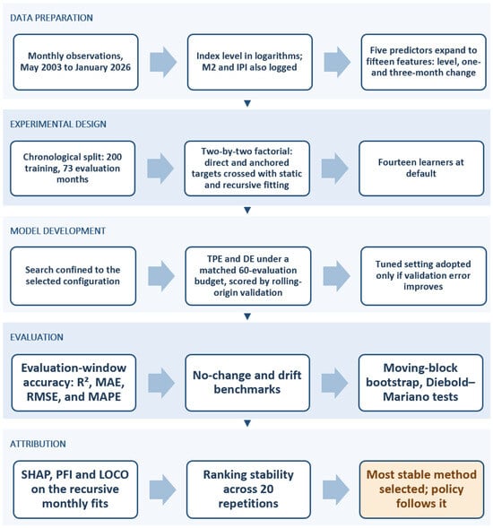
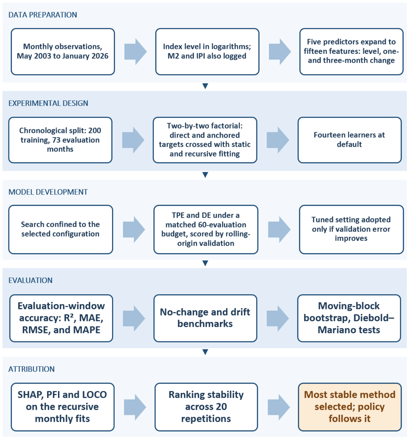
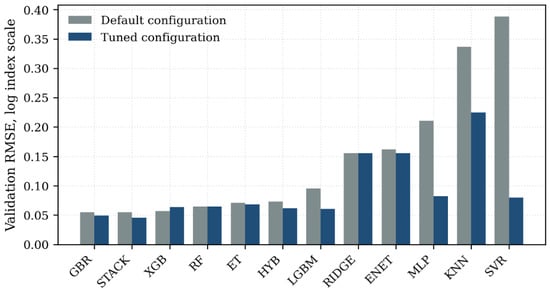
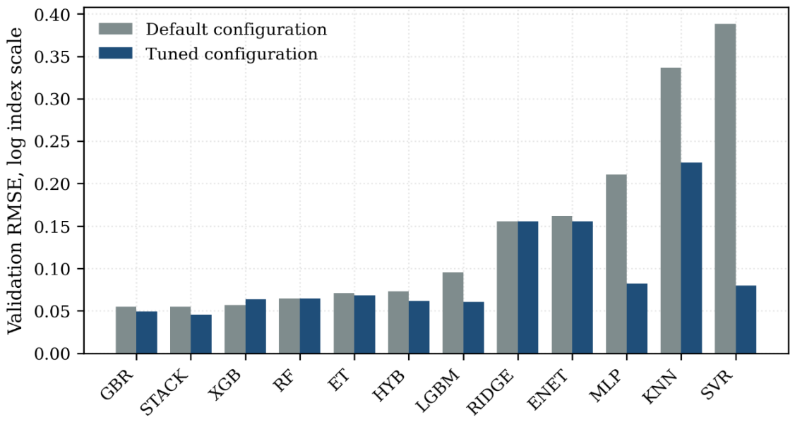
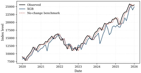
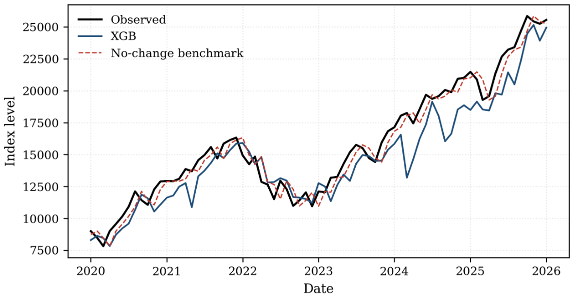
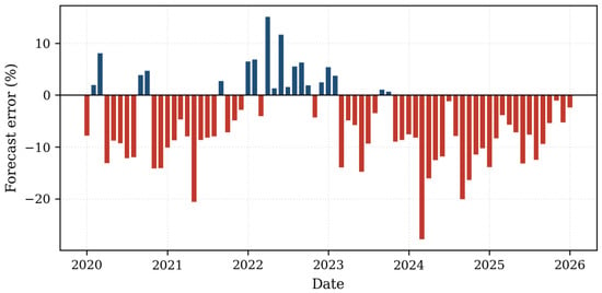
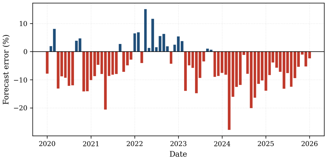
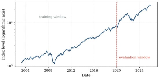
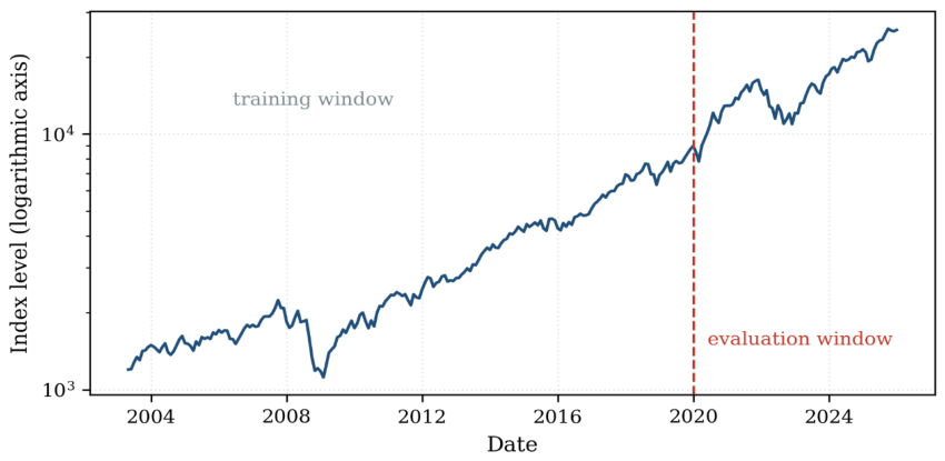
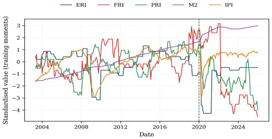
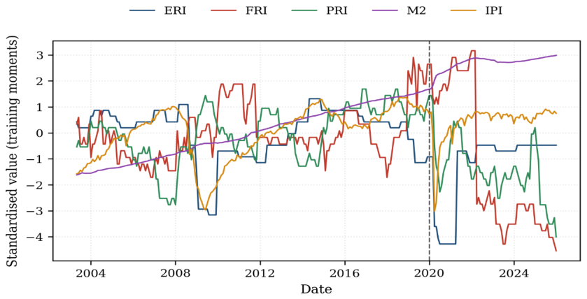
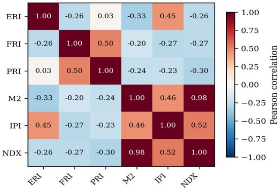
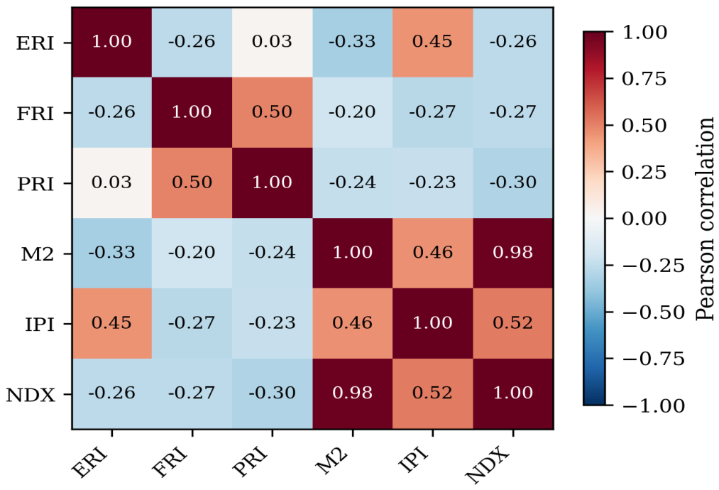
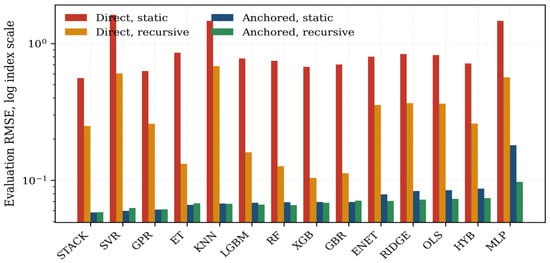
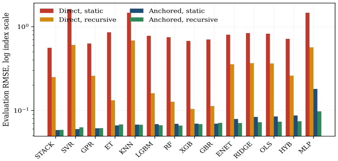
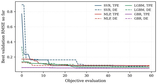
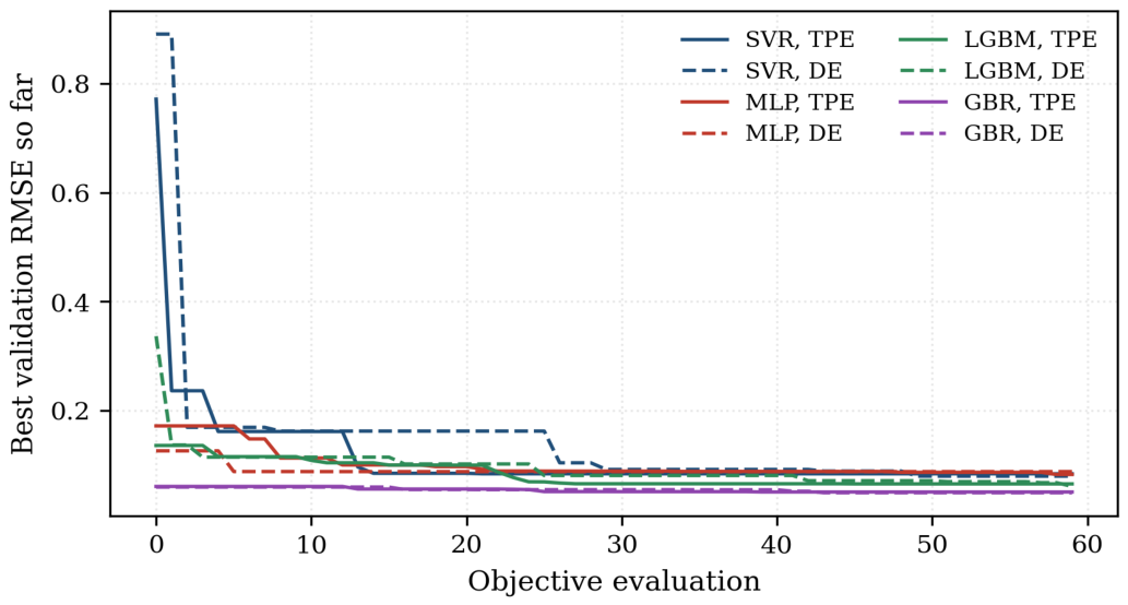
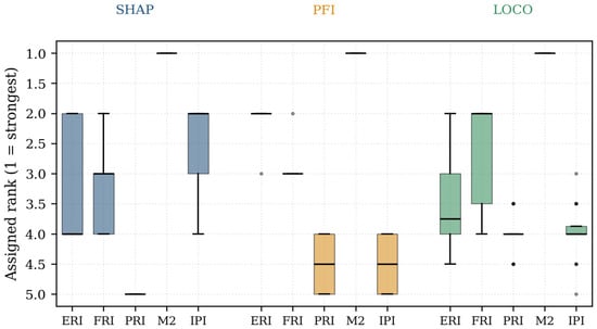
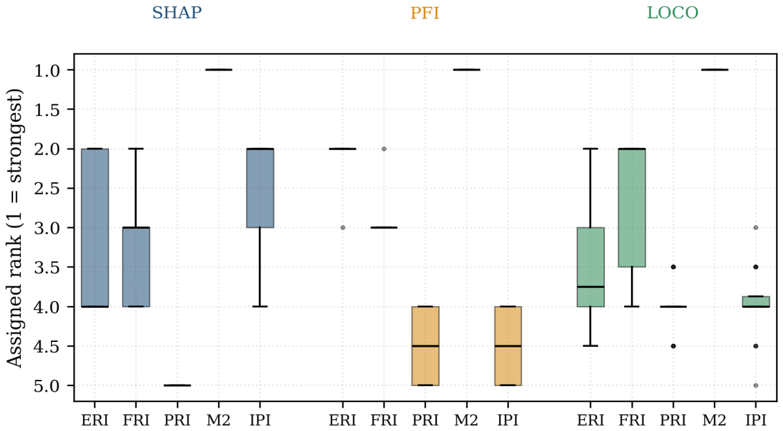
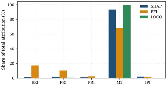
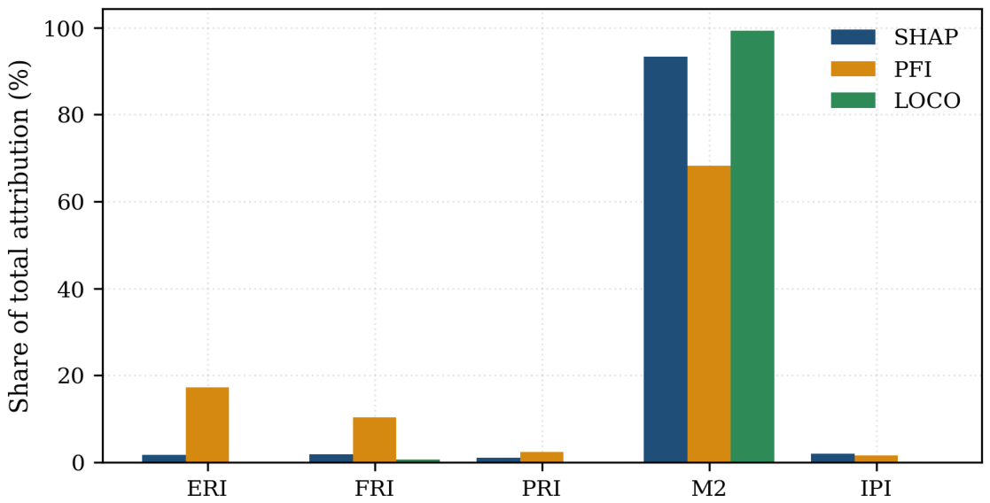

Disclaimer/Publisher’s Note: The statements, opinions and data contained in all publications are solely those of the individual author(s) and contributor(s) and not of MDPI and/or the editor(s). MDPI and/or the editor(s) disclaim responsibility for any injury to people or property resulting from any ideas, methods, instructions or products referred to in the content. |
© 2026 by the authors. Licensee MDPI, Basel, Switzerland. This article is an open access article distributed under the terms and conditions of the Creative Commons Attribution (CC BY) license.