


Abstract
Climate change is increasingly seen as a risk to the economy and financial systems. This is because weather patterns can affect how much people produce, inflation, trade, investment and how well the financial sector performs. These effects are especially important in developing countries that are sensitive to climate change. Even though there is growing research linking climate and finance, there is still no solid evidence on how climate, economic factors, and financial development are connected in South Africa. This study looks at these links using data from 1972 to 2023. It focuses on financial-sector development, which is measured by the amount of credit given to the private sector as a share of GDP. The study also includes other factors: total annual rainfall, temperature, trade openness, inflation and human development. To analyse the data, the researchers use the ARDL model developed by Pesaran, Shin and Smith in 2001. This model helps to find both long-run relationships and short-run movements between the variables. The results show a long-run relationship among the variables in the model. In this term, trade openness has a negative and statistically significant effect on financial-sector development (coefficient = −1.7548, p = 0.0260). Inflation also has a significant effect (coefficient = −0.0207, p = 0.0128). Temperature is positively and significantly associated with financial-sector development in the model (coefficient = 11.0507, p = 0.0098), but this result should be interpreted with caution. This is because temperature was transformed using a logarithm and measured in degrees Celsius, and there could be shared long-term trends affecting the results. Rainfall and human development do not show significant long-term effects. In the run, improvements in human development are positively and significantly tied to changes in financial-sector development (coefficient = 5.0723, p = 0.0005). Inflation changes also have a significant short-run effect (coefficient = −0.0152, p = 0.0005). The short-run effect of trade openness is not statistically significant. The error-correction term is negative and significant (−0.3513, p < 0.001), meaning that 35.1% of any imbalance from the long-run equilibrium is corrected within one year. Overall, the findings suggest that climate, macroeconomic and financial factors are linked in South Africa but not through strong structural causes. Instead, the relationships appear to be conditional and influenced by a mix of factors.
1. Introduction
Financial-sector development is crucial to economic growth, investment, credit allocation, risk management, and shock transmission mechanisms. The financial sector, however, operates within a changing business environment in climate-sensitive economies, characterised by higher inflation, changing trade conditions, production losses, climate-related pressures, and greater uncertainty. Climate change is thus increasingly seen as a macroeconomic and financial risk with implications for productivity growth, inflation dynamics, labour markets, trade performance, and the condition and resilience of the financial sector (Dafermos et al., 2018; Adekomaya et al., 2025).
The economic impact of climatic shocks is greater, especially in developing countries and emerging markets, due to the simultaneous effects of climate-sensitive productive activities, institutional constraints, poverty, and the economy’s adaptive capacity. In Africa, agriculture, mining, manufacturing, energy production, and household livelihoods remain increasingly vulnerable to changing temperatures, altered precipitation, droughts, floods, and other climatic factors. The repercussions of these conditions may include shifts in loan demand, borrowers’ ability to repay loans, investment behaviour, liquidity requirements, and uncertainty in the macroeconomic environment within which financial systems operate. However, the dynamic relationships linking climatic conditions, macroeconomic variables, and financial-sector development in Africa remain poorly understood.
South Africa provides an important context for examining these relationships. The country has a relatively developed financial sector and remains heavily reliant on climate-sensitive industries such as agriculture, mining, manufacturing, and energy production. Climatic conditions thus can coincide with shifts in inflation, trade conditions, economic activity, and financial practices. Although there is growing awareness of the financial risks of climate change, empirical research in South Africa investigating the Linkages among climatic conditions, macroeconomic conditions, and financial-sector development remains rather limited in both the extent and duration of the studies.
Understanding these relationships is also relevant to sustainable development. The resilience of the financial sector affects investments, productive enterprises, adaptation, and overall economic stability; economic pressures associated with a changing climate may contribute to financial vulnerability and constrained financial intermediation. The study thus has relevance to the wider goals of Sustainable Development Goal 8—sustainable and inclusive economic growth—as well as Sustainable Development Goal 13, which encourages the strengthening of responses to climate-related risks. This climate–macro–financial nexus is especially relevant to economies like South Africa, where sustainable development hinges on both the macroeconomic stability and the financial system’s ability to perform in a climate-changing environment.
Another important consideration concerns the interpretation of financial-sector expansion amid climatic and macroeconomic stress. Increased domestic credit can indicate productive deepening, but it could also reflect greater credit and liquidity needs amid economic uncertainty. These mechanisms are not differentiated in the present empirical design. Therefore, the possibility that financial expansion is partially related to stress-related adjustment is considered an interpretive hypothesis rather than an empirically tested phenomenon. This distinction serves as a foundation for future research by introducing more disaggregated indicators of credit composition, credit quality, household credit taking, corporate credit taking, and financial risk.
With this backdrop, this study revisits the short- and long-run links between key macroeconomic variables, climate and financial-sector development in South Africa using annual time-series data. Financial-sector development is proxied by the ratio of domestic credit to the private sector to GDP. At the same time, the explanatory variables in the estimated model are temperature, rainfall, trade openness, inflation, and human development. The study utilises the methodology of Pesaran et al. (2001) based on the ARDL framework, which allows estimation of long- and short-run equilibrium relations and short-run dynamics for variables with unit-root and non-integrated properties, provided there is no unit-root variable among them.
The study makes three main contributions to the climate–finance literature. First, it offers evidence from climate drivers and macroeconomic indicators in a relatively consistent time-series framework across South Africa, providing insights into their interdependence specific to the South African context. Second, by using the ARDL methodology, it is possible to distinguish between long-run equilibrium relations and short-run adjustment processes, and hence obtain evidence on the nature of the relationship between financial-sector development and climatic and macroeconomic conditions across different time horizons. Third, instead of taking the established empirical pathways of the climate’s influence at face value, the study enquires into the important wider literature on climate and macro-economic risk, or financial intermediation. Therefore, the analysis provides evidence of conditional climate–macro–financial associations, while acknowledging that the underlying transmission mechanisms within the triple association require further empirical exploration.
The rest of the paper is structured as follows: Section 2 presents a literature review that develops the study’s conceptual positioning. The description of the data, variables, model specifications, and econometric methodology is provided in Section 3. The empirical results, Unit root tests, ARDL Bounds Test, Long-run and short-run estimates, diagnostic tests and Additional Predictive analysis are presented and discussed in Section 4. The policy implications are given in Section 5, and the conclusions and further studies are given in the last section of the study.
2. Literature Review
2.1. Theoretical Literature
2.1.1. Climate–Macroeconomic Risk Theory
The climate–macroeconomic risk theory offers a theoretical framework for understanding the interaction between macroeconomics and financial characteristics in response to climate shocks. Climate change is increasingly recognised as a serious economic risk, in addition to being an environmental issue, and it can be linked to variations in economic productivity, inflation, trade results, investment environment, and financial stability. Recent droughts, floods, heatwaves and rising temperatures, combined with other climate pressures, have heightened concerns about the vulnerability of the macroeconomy in developing and emerging economies, where structural inequalities, institutional limitations and high sensitivity to climate-sensitive sectors are present.
There are possible macroeconomic channels linking climatic influences on economic and financial conditions, as identified in the theoretical literature. For instance, climate risks may exacerbate the vulnerabilities of climate-sensitive sectors, such as agriculture and energy, thereby affecting overall economic activity and macroeconomic stability, as supported by Adekomaya et al. (2025). These impacts could manifest as reductions in production, supply issues, greater production and economic costs and economic uncertainty. These channels will be investigated as theoretical channel transmission mechanisms in the present study, rather than estimated directly via the empirical model.
Commonly used assessment tools for climate risk analysis focus on three interlinked aspects: exposure, sensitivity, and adaptive capacity. Government exposure to climatic risks is not uniform across economies, as some countries are highly exposed and sectors closely related to climate are significant in their economies. At the same time, those with relatively small adaptive capacity may be more vulnerable to the impacts of climatic shocks. This is the more general theoretical framework for examining how climatic conditions relate to productivity, investment, employment, consumption, and financial conditions.
An insight into one possible macroeconomic path concerns productivity. Higher temperatures and extreme heat can reduce labour productivity and work capacity, particularly in climate-exposed activities such as agriculture, construction, mining, and other forms of outdoor production (Levi et al., 2018). This loss of productivity can lead to reduced output capacity, shifting business expenses, and growing financial insecurity. Some important sectors in South Africa remain vulnerable to climatic conditions, and such mechanisms are relevant.
A further potential issue relates to inflation/supply-side pressures. Agricultural production, food systems and energy supply failures or conditions due to climate change could affect production costs and price dynamics. According to Melaku (2020), the money supply, exchange rate changes, import prices, and output dynamics are among the significant factors that affect inflation in Africa. Climatic shocks can thus interact with these prevailing macroeconomic pressures through their impacts on production and supply conditions. The current study, however, does not directly estimate a causal climate-to-inflation channel; rather, inflation is included as a separate macroeconomic variable that may be associated with financial-sector development.
On a macroeconomic level, there is value in adopting a climate–macroeconomic risk theory perspective to at least partially understand the different economic channels linking climate and financial-sector outcomes. The purpose of this study is to apply the theory of motivation variables by including climatic and macroeconomic variables, and to ensure that the associations found in the estimated study are associated with financial-sector development. The theoretical framework does not suggest that the ARDL model will identify each one of the ARDL’s transmission mechanisms. This separation is critical in the context of South Africa’s climate-sensitive sectors, coupled with unemployment, long-standing inequality, energy insecurity, and overall macroeconomic fragility.
2.1.2. Financial Intermediation Theory
The financial intermediation theory seeks to answer questions about the role of financial institutions in mobilising savings and allocating credit, managing risk, and facilitating economic activity. The theory of traditional financial intermediation mainly focuses on the role of financial intermediaries in reducing transaction costs and information asymmetries. Banks and financial institutions thus play their part in promoting economic activity by providing credit facilities, liquidity, risk-spreading, and the mobilisation of financial resources.
Financial intermediation has also been found to be responsive to institutional forces and macroeconomic conditions, in line with the literature. Inflationary conditions, liquidity, uncertainty, credit demand, and regulatory conditions can affect financial institutions’ behaviour and shape the distribution of credit in the economy. In this logic, financial-sector development encompasses not only the growth of credit but also the broader financial-sector institutional context in which financial intermediation operates.
The review paper by Goodfriend and McCallum (2007) builds on the classic financial intermediation framework by introducing banking-sector liabilities, banking-sector liquidity conditions, collateral constraints, and financial confidence into macroeconomic adjustment processes. Their structure captures the dynamics between financial conditions and the macroeconomy. Climate-sensitive scenarios imply that, within a climate context, the various mechanisms outlined above may modify repayment capacity, collateral quality, liquidity demands, financial uncertainty, and credit conditions in tandem (or not) with economic disruptions stemming from a climatic shock.
In the present study, FIT serves primarily as an interpretive framework for the relationships among the various climatic and macroeconomic variables used in the empirical model and financial-sector development. The theory does not argue that the ARDL specification exhaustively identifies the underlying complete banking-accelerator mechanism or the underlying channels identified by Goodfriend and McCallum (2007). Instead, it offers conceptual support for understanding the association between a shift in financial-sector adjustment in South Africa and shifts in climatic and macroeconomic conditions.
2.1.3. Integrated Climate–Financial Framework
This study brings together elements of climate–macroeconomic risk theory and financial intermediation theory, embedding them in a more encompassing climate–financial framework (Figure 1). The framework aims to provide conceptual arguments for potential links between climatic conditions and financial-sector outcomes through various economic pathways. These channels are conceptual, and not all are directly estimated in the empirical model.
Figure 1.
Climate–Macroeconomic Transmission Framework. Source: Authors’ own conceptualisation based on Goodfriend and McCallum (2007), Dafermos et al. (2018), and West and Brereton (2013). Note: The framework illustrates theoretical transmission channels. The empirical ARDL model directly estimates associations between financial-sector development and selected climatic and macroeconomic variables; it does not separately estimate all intermediate transmission mechanisms shown in the framework.
The framework regards climatic conditions as external environmental factors that could influence climate-sensitive sectors such as agriculture, mining, manufacturing, and energy generation. In principle, such sectoral impacts could relate to changes in productivity, production costs, inflationary pressures, trade conditions, household welfare and economic uncertainty. Shifts in liquidity levels, financial risk, financial inclusion, debt-servicing capacity, and credit demand can then parallel the consequential macroeconomic shifts.
Within the South African context, these relationships are particularly relevant, as climate-sensitive sectors are set against the backdrop of chronic unemployment, inequality, energy insecurity, and other macroeconomic challenges. Increased domestic credit growth under these conditions may therefore be a sign of rising demand for credit and liquidity during economic trouble, as well as of financial deepening in the economy. The present empirical design does not make any specific separation between these mechanisms. Thus, the idea that there is a difference between the welfare-enhancing aspects of financial deepening and financial adjustment in response to stress is treated as a theoretical interpretation and a hypothesis for future studies, rather than an empirically established result.
This integrated framework thus offers a conceptual basis for understanding the estimated relationships among climatic conditions, macroeconomic variables and financial-sector development. It does not provide a second-round effect of climate shock, which links them to financial-sector issues mediated by inflation, productivity or trade. Rather, these pathways are considered theoretically viable and warrant further empirical investigation, particularly through mediation models, systems approaches, interaction patterns, and/or more specific financial metrics.
2.2. Empirical Literature
2.2.1. Climate Change and Financial Systems
The risk of climate change as a systemic macroeconomic and financial risk is gaining recognition and traction across financial institutions, capital markets, investment patterns, and macroeconomic stability. The literature on climate finance often categorises risks into physical risks, which are linked to exposure to climate hazards, and transition risks, which are linked to shifts in climate policy, decarbonisation, environmental regulation, technological change, and structural economic adjustment.
Climate-related financial risks can materialise as physical, productivity, or transition risks and can impact asset values, financial risks, and macroeconomic stability, according to a 2018 study by Dafermos, Nikolaidi, and Galanis. These mechanisms reflect the idea that environmental shocks could interact with financial conditions through changes in economic performance, investment, or risk exposures.
Along the same lines, Carè (2023) highlights several topics in the climate-finance literature: climate disclosure, systemic financial risk, climate resilience, and the measurement of climate risk. However, this research is scattered across the fields of finance, environmental economics, accounting, and macroeconomic research, thereby hindering a complete synthesis to quantify and build climate-related financial risk.
Financial regulators have also repeatedly incorporated climate risk considerations into their financial governance frameworks. Omeir and Vasiliauskaitė (2025) explore how climate stress tests, disclosures, and macroprudential measures are emerging as viable tools for better understanding institutional vulnerability and enhancing financial resilience amid the risks posed by various climate scenarios.
Overall, the available empirical studies indicate that the connection between climate-related risks and financial system outcomes may be mediated by theoretically possible channels, such as effects on productivity, transition uncertainty, institutional vulnerability, or changes in macroeconomic conditions. Nevertheless, the interpretation of these mechanisms should be approached with caution, as they are not directly identified in the present ARDL model. The time series analysis is conducted simultaneously for the climatic and macroeconomic variables, with the underlying transmission channels inferred from the broader literature on the connections among climate, the economy, and finance.
However, there is still limited empirical evidence available in the South African context. Previous studies have focused mainly on the effects of financial vulnerability to warming on business finance, and few have applied long- and short-run time-series analyses to link economic and climatic change to the development of the financial sector. This offers empirical justification for the present research.
2.2.2. Climate and Inflationary Transmission
Climate change might interact with economic and financial outcomes through macroeconomic channels, such as inflation. Climatic shifts in the production and supply of food, energy, and labour can exert upward or downward pressure on prices and macroeconomic conditions, particularly in the beef market. Climate-sensitive economies are especially sensitive to the effects, as agricultural production, energy systems and inputs are at risk from climate and external shocks.
Climate-related shocks and stressors to agriculture and energy markets can lead to macroeconomic instability through shifts in production expenses and prices, especially in climate-sensitive economies, as argued by Adekomaya et al. (2025). From an economic perspective, the monetary basis of inflation may affect real returns, borrowing costs, investment, financing, and the intensity of use of financial intermediation.
Climate-induced price pressures can manifest in various ways, including disruptions to food supply, changes in energy markets, productivity losses, and disruptions to domestic and international supply chains. The intensity and duration of these impacts, however, will rely on the type of climatic shock, the structure of the economy, policy reaction, and prevailing macroeconomic conditions.
In the current research, inflation is thus treated as an independent macroeconomic variable that may be correlated with financial-sector development. The empirical model does not directly address the effect of climatic conditions on inflation or the possibility that inflation serves as a mediator between climatic conditions and financial sector outcomes. In this view, the climate–inflation relation is treated as a theoretical relationship rather than a causal link, as implied by ARDL estimates.
2.2.3. Climate and Financial Stability in Africa
Since Climate change has increasingly become a major macroeconomic and financial stability issue in African economies, many African countries still rely on climate-sensitive sectors, and structural vulnerabilities in socioeconomic contexts, coupled with institutional changes, low adaptive capacity, and inadequate climate finance, can exacerbate their vulnerability to economic climate shocks.
Since the beginning of the climate–finance literature in Africa, the fields of disclosure, ESGs, climate-risk frameworks and macroprudential approaches to climate change have gained growing focus. Research on macro-financial dynamics, however, remains relatively scattered, with most existing studies focusing mainly on climate vulnerability, environmental policy, emissions, and impacts on specific sectors rather than on macro-financial dynamics.
Several sectors in Africa could be affected by climate-related pressures, including agriculture, energy, trade, and financial markets. All of this can happen simultaneously through production conditions, interest rates, investment activity, credit availability, and financial risk. However, the empirical evidence on the dynamic short- and long-run links among climate, macroeconomic variables, and financial sector development in African economies remains limited.
The financial impact of climate pressures could vary significantly by country, depending on financial depth, financial institutions, economic and institutional structures, adaptive capacity, and exposure to climate-sensitive sectors. Given this background, the African context provides a robust foundation for examining the linkages between climate, macroeconomic, and financial outcomes, while acknowledging significant cross-country variability.
2.2.4. Climate and Financial Stability in South Africa
Climate change is increasingly recognised as a potential macroeconomic and financial risk in South Africa. The nation has a relatively advanced financial system, but still relies heavily on climate-vulnerable sectors such as agriculture, mining, manufacturing, and energy production. The interaction between climatic pressures and existing macroeconomic weaknesses, such as inflation, energy shortages, unemployment, inequality, and external-sector vulnerabilities, could thus heighten vulnerability.
While policies and academia increasingly focus on the financial risks posed by climate change, the empirical literature in South Africa on the dynamic link between climate and financial-sector development is relatively sparse. The current literature has been limited to studying climate vulnerability, environmental and regulatory policies, corporate disclosure, sector-specific climate effects, and overall financial risk. It has investigated climate–macro–financial relations using dynamic time-series analysis at a few short- and long-duration stages.
The economic impact of climate change can manifest in the financial system in several ways, including reduced productivity, constrained investment potential, weakened repayment capacity, asset value declines, increased demand for liquidity, inflation, and trade impacts. These mechanisms, however, are not to be confused with relational mechanisms that can be directly identified empirically. Climatic and macroeconomic factors are jointly used as proxies in the ARDL model, so this study does not directly examine the subsequent steps in the transmission of climate to financial-sector development.
Climatic exposure combined with a unique economic and financial configuration is of particular relevance in South Africa. A key aspect of country-specific relevance is the availability of climate–finance evidence from the South African context that is both directly relevant and directly comparable to the experiences of African countries. Moyo and Wingard (2015) provide such evidence for South Africa, thus offering a useful country-specific explanatory context for the climate–finance relationship in Africa. The current research builds on this broader body of research. It investigates the dynamic long- and short-term relationships among climate, macroeconomic indicators, and financial sector development at the national level.
As a whole, there is a significant knowledge deficit in the South African literature regarding dynamic macro-financial analysis of climatic conditions and financial-sector development. To tackle this, empirical approaches must clearly distinguish between direct estimation and the introduction of theoretically induced transmission links, especially when the transmission channels related to climate change are not directly estimated, such as through inflation, productivity, or trade.
2.3. Literature Gap and Conceptual Positioning
While climate change is slowly attracting greater attention as a systemic macroeconomic/financial risk, there are significant gaps in the literature. First, climate economics and macro-financial research remain surprisingly segmented, with many studies focusing on climate sustainability and others on financial stability, but little work to date exploring the joint effects of climate conditions, macroeconomic policies, and financial-sector outcomes within a unified empirical analysis.
Second, empirical studies on climate–finance are mainly conducted in developed countries and far less in emerging countries, particularly in climate-sensitive ones such as South Africa. This is significant given that the economic and financial impacts of climate change could vary by institutional capacity, financial depth, economic structure, inequalities, and climate-sensitive sectors.
Third, the short- and long-run relationships between climatic conditions and the development of South Africa’s financial sector are relatively little known. Empirically, on a few dimensionally different channels through which productivity could drive inflation, trade, liquidity, and financial risk (or direct reversal) are not always closely tested. The key contribution of the present study is therefore to estimate conditional relationships among climatic conditions, selected macroeconomic factors, and financial-sector development; it is not a study that claims to exhaustively trace the underlying sequence of transmission mechanisms.
Another conceptual problem is how to interpret the expansion of financing in a climate- and macroeconomic-stress scenario. Financial activity might be a good sign of financial deepening. Still, it could also correspond to higher credit demand, liquidity demand, insurance needs, and demand for risk-management instruments during uncertain economic times. Currently, there is no empirical design that explicitly separates these mechanisms. In this regard, it is considered a theoretical interpretation and an object of future empirical investigation, rather than an established empirical fact, that welfare-enhancing financial development differs from stress-related financial adjustment.
In this context, the study makes a significant contribution by providing time-series evidence for South Africa on the long-run relationships among trade openness, inflation, human development, and financial-sector development, as well as the short-run dynamics of these relationships. The conceptual framework is offered as an interpretation of these associations in the mainstream of the literature available in the fields of climate, macro and financial linkage, while ensuring a separation between any direct linkage of the environment hypothesised in the ARDL system and any linkage that is still theoretically plausible but has not been tested empirically in the present study.
3. Data and Methodology
3.1. Data Source and Study Period
The Empirical analysis is conducted using South African annual secondary time series data from 1972 to 2023. This time interval represents 52 calendar years, but the frequency of observations used for empirical estimation is influenced by the lag periods of all variables and by observations lost during the transformation to normality. So the nominal study period may be shorter, while the effective estimation sample may be smaller due to lagged observations and data transformations used in the dynamic specification.
This selected period reflects key structural and institutional, macroeconomic and environmental shifts in the South African economy: the late-apartheid economy, economic and financial-sector liberalisation after 1994, the 2008 global financial crisis and the growing significance of policy and economic risks due to climate events. Another advantage of a long period, which is also applicable to the annual time frame, is the ability to capture the long-run relationships among climatic, macroeconomic, and financial variables, as well as to estimate the long-run equilibrium relationships within the ARDL model.
The study uses secondary data from nationally and internationally accepted sources, such as the South African Reserve Bank (SARB), depending on the specific variables; in this instance, the World Development Indicators (WDI), the Climate Change Knowledge Portal, and Federal Reserve Economic Data (FRED). Information on the definition, unit of measure, and transformation of each variable is reported in the variable-definition table to enhance transparency and reproducibility.
3.2. Justification for Climatic Variables
Climatic variables such as temperature and rainfall are selected for the study because they serve as indicators of climatic conditions and their economic importance in production, natural resource availability, and the performance of production sectors. Including them does not capture all climate risk exposures, such as extreme events, drought severity, or exposures that vary across space.
The temperature used as an indicator is the average annual surface air temperature (°C). Temperature variations can also impact labour productivity, agricultural output, industrial production, and energy demand, especially for climate-sensitive sectors (Aragón et al., 2021; Ziervogel et al., 2014). Temperature-related pressures can thus be expected to occur simultaneously with changes in production conditions and other macroeconomic pressures in the South African context.
Total annual precipitation, measured in mm, quantifies rainfall. This variable represents precipitation conditions on an annual time scale only. It should not be viewed as a direct indicator of rainfall variability, drought severity or length, rainfall anomalies, or extreme rainfall. Annual precipitation can, however, help indicate general trends in changes in water availability and production conditions for climate-sensitive activities such as water use in agriculture, industry, and food production (Blignaut et al., 2009; Orimoloye, 2022).
There are also other constraints related to the use of annual national climate measures. Average values across the country may mask considerable variability between regions and from season to season, and annual rainfall amounts do not adequately represent the timing, intensity, and intra-annual variability of rainfall. Climatic variables should therefore be viewed as general proxies for national climatic conditions, and not as climate shocks or extreme-weather exposure.
3.3. Variable Specification and Theoretical Justification
3.3.1. Dependent Variable
Financial Sector Development (FS)
The development of the financial sector is measured by domestic credit to the private sector as a percentage of GDP. It measures the share of credit extended to the non-financial private sector relative to the economy’s overall size. It is commonly used as an indicator of financial intermediation and financial depth. An increase in the domestic financial system’s role in allocating funds to firms and households is reflected in higher domestic credit to the private sector. It is called LFS in the empirical estimation, corresponding to the variable that is transformed using the logarithmic transformation.
3.3.2. Independent Variables
Temperature (TEMP)
Average annual surface air temperature (°C) is used to measure temperature. Temperature is included because climate conditions may trigger changes in labour productivity, agricultural production, manufacturing production and energy demand, especially in climate-sensitive sectors (Ziervogel et al., 2014; Aragón et al., 2021). It can then affect broader macroeconomic sectors that are important to the financial sector’s health.
Rainfall (RF)
Annual precipitation is measured as total annual rainfall and is represented in millimetres of water. The variable reflects general year-to-year precipitation patterns, not precipitation variability, drought severity, rainfall anomalies, or extreme precipitation events. Water availability, agricultural production, industry, and food systems can be affected by annual precipitation (Blignaut et al., 2009; Orimoloye, 2022). The coefficient, therefore, reflects the relationship between overall annual precipitation and the growth of the financial sector, rather than the impact of precipitation variability over the years.
Trade Openness (TO)
The level of openness of trade is calculated as the sum of total exports and imports, divided by GDP. It reflects the level of integration of South Africa’s economy into the international economy and the vulnerability to external economic factors. The theoretical link between openness to trade and the development of finance is unclear. Improved economic integration can benefit financial integration by naturally pursuing greater economic activity, investment and demand for finance. In contrast, financial external exposure may exacerbate the impact of external shocks and changes in financing conditions.
Inflation (INF)
Inflation is measured as the annual percentage change in consumer prices. It is incorporated because it negatively affects real returns, uncertainty, borrowing and investment decisions, and the efficiency of financial intermediation (Shabir et al., 2025; Regmi, 2008). In general, there should be a negative correlation between inflation and financial sector development.
Human Development Index (HDI)
The HDI represents three general indicators of human development: Life expectancy, knowledge, and income. Improved financial-sector development can be linked to higher levels of human development, as manifested in higher income levels, financial skills, access to financial markets, and a greater number of financial services used by the population (Lawn, 2007). If a logarithmic transformation is applied to the empirical model, the variable is called LHDI (Table 1).
Table 1.
Variable Definitions and Measurements.
3.4. Functional Relationship and Model Specification
Model specification constitutes an essential component of econometric analysis because it defines the relationship between the dependent variable and explanatory variables based on theoretical and empirical considerations.
The financial sector model is specified as follows:
where
- = Financial sector indicator proxied by domestic credit to the private sector (% of GDP);
- = Mean annual temperature;
- = Total annual precipitation;
- = Trade openness;
- = inflation;
- = Human Development Index;
- = Intercept term;
- to = Slope coefficients;
- = Stochastic error term.
The explanatory variables are chosen based on the climate, macro, financial, and financial-intermediation literature. Temperature and rainfall data are included to represent climatic conditions, and human development indicators, alongside trade openness and inflation, are included to represent macroeconomic and socioeconomic conditions affecting the development of the financial sector. The model includes estimates of the conditional relationships between these variables and financial-sector development. It does not directly model the channels of transmission along which the climate might affect inflation, productivity, trade or other macroeconomic variables.
3.5. Analytical Technique
The study uses the autoregressive distributed lag (ARDL) modelling framework developed by Pesaran et al. (2001). This is quite suitable, since the ARDL approach allows estimation of long-run equilibrium relationships and short-run adjustment dynamics within a single reduced-form framework.
There are some advantages to the ARDL model. Firstly, it is ideal for relatively small annual time-series samples and does not require the large samples typically needed by some traditional cointegration methods to estimate dynamic relationships. This is especially important for the present study, which utilises a relatively small annual time-series sample.
Second, the ARDL methodology is applicable when the variables are integrated of order zero (I(0)), order one (I(1), or a mixture of both, if none of the variables is integrated of order two (I(2). So, the integration properties of the variables are important prerequisites to be determined before running the ARDL bounds-testing procedure.
Third, the ARDL framework can be presented in an error-correction form if a long-term relationship exists, as it separates short-run movements from long-run adjustment processes. To measure the rate of error correction towards the LR equilibrium after short-run shocks, the error-correction term is used (Duasa, 2007).
The estimation procedure used is the ARDL model, estimated as a single-equation dynamic specification. Therefore, the coefficients estimated in this study should be considered conditional, rather than causal, relationships between financial-sector development and the variables used in the study. This interpretation is especially relevant when financial-sector development is coupled with feedback on certain explanatory variables.
ARDL EQUATION
where
- = First-difference operator;
- = Error correction term lagged by one period;
- = Speed of adjustment coefficient;
- = White-noise error term.
3.6. Estimation Procedure
3.6.1. Descriptive Statistics
The empirical analysis begins with descriptive statistics to characterise the distributional properties and general behaviour of the variables used in the study (Nick, 2007). The descriptive analysis summarises statistics on the central tendency, dispersion, skewness, and kurtosis of the data. It provides preliminary information about the statistical properties to be estimated at the formal level of time-series calculation.
3.6.2. Unit Root Testing
Gujarati and Porter (2009) suggested that, before any time series analysis, the stationarity characteristics of the variables involved must be assessed to minimise the possibility of spurious regression. Unit root tests, known as the Augmented Dickey–Fuller (ADF) and Phillips–Perron (PP), are conducted on each variable to test its order of integration.
The null hypothesis for both tests is that the series has a unit root; if the null is rejected, the series is found to be stationary. To determine whether the variables are integrated of order zero (I(0)) or order one (I(1)), these tests are performed as needed. Special focus is paid to ensuring that none of the variables is integrated of order two, I(2), because the ARDL bounds-testing procedure is not valid if one or more variables are I(2).
The empirical results, the deterministic part of the estimates, and the lag selection used in both tests are reported alongside them to make the stationarity test transparent.
The ADF equation is specified as follows:
The Phillips-Perron test is represented as:
The null hypothesis in both tests states that the variable contains a unit root. Rejection of the null hypothesis implies that the data are stationary. The reported temperature stationarity test is based on TEMP, whereas the final ARDL specification employs the logarithmically transformed temperature series, LTEMP. Because the transformed series was not retested separately, this inconsistency is acknowledged as a limitation of the pre-estimation analysis.
3.6.3. Lag Length Selection
The choice of the lag value is crucial in dynamic time-series modelling, as the model may otherwise suffer from inefficient estimation and residual autocorrelation. The optimal lag structure is then obtained by applying information criteria, such as the Akaike Information Criterion (AIC), Final Prediction Error (FPE), Schwarz Information Criterion (SC), and Hannan–Quinn Information Criterion (HQ), as well as the sequential likelihood-ratio criterion, if applicable.
Model selection for the final ARDL model specification is based on the following characteristics: model fit, model parsimony, and model diagnostic adequacy. The maximum lag length used and the information criterion adopted to develop the final ARDL model specification are reported along with the empirical results. The final ARDL(1,0,1,1,1,0) specification has been retained exactly as originally estimated. The manuscript has been revised so that it no longer states that selection details are reported where they are not available. No retrospective lag-search exercise has been introduced because this would require a new estimation procedure rather than clarification of the reported model.
3.6.4. ARDL Cointegration and Estimation
Once the appropriate lag order has been established and the variables’ integration properties are known, estimation of the ARDL model begins. A long-run equilibrium relationship between the variables is tested using the bounds test developed by Pesaran et al. (2001).
The null hypothesis of the bounds test is that no long-run relationship exists among the variables. When the calculated F-statistic exceeds the upper-bound critical value, the null hypothesis of no cointegration is rejected, indicating evidence of a long-run relationship. When the F-statistic falls below the lower-bound critical value, the null hypothesis cannot be rejected. If the F-statistic lies between the lower and upper bounds, the result is inconclusive.
The bounds test is used to interpret the study’s results, but (asymptotic) critical-value theory limits should be considered, given the relatively small annual sample size. Given the relatively small annual sample, the conventional asymptotic bounds are interpreted cautiously, and the bounds-test evidence is not treated as definitive in the absence of finite-sample critical values.
After cointegration, the long-run coefficients and their short-run representation, along with the short-run error-correction term, are estimated. The error correction term represents how fast short-run deviations from the long-run equilibrium will disappear with time.
3.7. Diagnostic Tests
Once the forecasts have been made, post-estimation diagnostic tests are performed to test the fitness and reliability of the estimated ARDL model. Diagnostic testing is important because the validity of long-run and short-run estimates can be affected by changes in residual behaviour, the functional specification, and the stability of estimated model parameters (Gujarati & Porter, 2009; Pesaran et al., 2001).
The model is assessed for serial correlation, heteroskedasticity, normality of the residuals, multicollinearity, functional-form misspecification, and parameter stability.
3.7.1. Serial Correlation
The serial correlation of the residuals (Breusch–Godfrey Lagrange Multiplier test) is investigated (Gujarati & Porter, 2009). The null hypothesis is that the residuals are uncorrelated in time. The lack of rejection of the null hypothesis means that there is no statistically significant serial correlation at the given significance level.
3.7.2. Heteroskedasticity
The Breusch–Pagan–Godfrey test is one method for testing whether the residual variance is homoskedastic across observations (Gujarati & Porter, 2009). The null hypothesis is related to the residuals and is homoskedasticity.
3.7.3. Normality Test
The residual normality is assessed using the Jarque–Bera test (Jarque & Bera, 1987; Gujarati & Porter, 2009). The null hypothesis is that the residuals follow a normal distribution.
3.7.4. Multicollinearity
The Variance Inflation Factor (VIF) is an additional diagnostic for assessing the linear association among the explanatory variables. Given the dynamic nature of the ARDL model with lagged variables, the VIF findings should be interpreted with caution.
3.7.5. Functional Form Test
Some carry out the Ramsey RESET test to assess the functional specificity of the estimated model and to check for omitted nonlinear relationships and/or misspecified functional forms (Sapra, 2005). The null hypothesis is that the “correct” model is specified.
3.7.6. Stability Tests
Parameter stability is assessed using the Cumulative Sum of Recursive Residuals (CUSUM) test. The CUSUM test evaluates whether the recursive residuals remain within the 5% critical boundaries over the estimation period. Stability is indicated when the test statistic remains within these critical limits. The test provides evidence regarding recursive parameter stability but does not, by itself, rule out all possible structural breaks over the study period (Turner, 2010).
3.8. Robustness Checks
The robustness of the estimated model is evaluated mainly through post-estimation diagnostics and stability testing. These consist of tests that check whether there is serial correlation, heteroskedasticity, residual normality, multicollinearity, functional-form specification, or parameter instability.
The interpretation of the empirical results recognises potential sensitivity to model specification, lag structure, variable measurement, and the relatively small annual sample. Alternative specifications may provide useful additional robustness checks, particularly for the temperature variable and possible structural changes over the study period; however, these are not estimated in the present study. Alternative lag structures and specifications may be useful additional robustness checks, especially regarding the influence of the temperature variable and possible structural changes in the data over the study period.
To complement the assessment of the predictive relationships among these variables, Granger causality/block exogeneity Wald analysis based on VAR models is used. The results are not interpreted to infer the existence of a structural causality between variables, since relationships between the variables determined by the ARDL estimates do not guarantee their predictive causality.
3.9. Methodological Limitation
The ARDL technique is suitable for studying dynamic short- and long-term relationships, but the estimated coefficients should be treated as conditional associations rather than causal effects. Where there may be feedback effects between financial-sector development and some of the explanatory factors, this limitation is important.
Since the study used VAR models, the VAR-based Granger causality/block exogeneity Wald tests were also utilised as a complementary test for predictive relationships between the variables. However, the Granger causality results are interpreted as evidence of predictive precedence rather than structural or economic causation. A statistically significant result indicates that past values of one variable contain predictive information about another variable, but it does not identify the underlying causal mechanism.
Considering the nature of the integration of the variables used, the results obtained from the VAR-based Granger causality are carefully interpreted and presented as secondary evidence alongside the ARDL analysis.
4. Findings and Discussion: Financial Sector
4.1. Descriptive Statistics
The descriptive statistics of the variables used in the financial-sector model are reported in Table 2. The financial-sector indicator (LFS) in log format shows a standardised mean of 1.9350 and a standard deviation of 0.1592, indicating a moderate dispersion in the observed sample. Even lower and higher amounts of 1.6136 and 2.1450, though, suggest a fluctuation in the development of the financial sector over time.
Table 2.
Descriptive statistics.
The total annual precipitation or rainfall (RF), measured in millimetres, has a mean of 480.49 mm and a standard deviation of 77.86 mm. The series ranges from 319.80 mm to 687.21 mm, indicating considerable variation in total annual precipitation over the sample period. These statistics should be interpreted as variation in annual precipitation levels rather than as direct measures of rainfall variability, drought severity, rainfall anomalies, or extreme precipitation events.
As shown, the mean of trade openness (LTO) is 1.6765, with a standard deviation of 0.0648, while the mean of the Human Development Index (LHDI) is 1.7793, with a standard deviation of 0.0240. The relative dispersion of these variables shows only minor movement in international economic integration and human development over the sample period.
The value of the inflation variable (INF) is 8.9228, with a range of −0.6920% to 18.6549%, a mean of 8.9228, and a standard deviation of 4.4353. This relatively large spread implies considerable volatility in price increases from one year to the next during the sample period. The negative minimum value represents a period of consumer price decline, and the maximum represents periods of high consumer prices compared to other periods.
Temperature (LTEMP) is a logarithmic scale with a mean of 1.2551, a minimum of 1.2284, and a maximum of 1.2849. The standard deviation of 0.0122 is comparatively small, as was the case with the other variables. The values for the descriptive statistics should be used with caution, however, as the baseline temperature series is in degrees Celsius and has been transformed (logarithmically). The interpretation of temperature in terms of the economy is taken up on the empirical level in the subsequent analysis.
The Jarque–Bera probabilities suggest that rainfall, trade openness, human development, inflation, and temperature do not exhibit a significant departure from normality at the 5% significance level. The probability of 0.0621 is higher than 0.05 but less than 0.1, indicating that the LFS distribution should be used with some caution.
In summary, these descriptive statistics provide an initial overview of the variables’ distributional characteristics but do not establish causal or transmission relationships among climatic conditions, macroeconomic variables, and the development of the financial sector. Hence, the dynamic relationship among these variables is subsequently explored using the ARDL framework.
4.2. Unit Root and Stationarity Test
The Augmented Dickey–Fuller (ADF) and Phillips–Perron (PP) unit-root test findings for all the financial-sector variables are displayed in Table 3. The findings suggest that both I(0) and I(1) integration orders exist, with the requirement of the ARDL methodology that there should be no I(2) variables.
Table 3.
Unit-root test results (ADF and PP).
The non-stationary nature of both the financial-sector indicator (LFS) and trade openness (LTO) remains at the stationarity level. Still, they become stationary after differencing at both levels and I(1). The rainfall (RF) series is stationary according to the ADF and PP tests and is considered I(0).
The temperature variable (TEMP) is stationary according to both the ADF and PP tests. However, the final ARDL specification employs the logarithmically transformed temperature variable, LTEMP. Because the unit-root test was conducted on TEMP rather than LTEMP, the stationarity evidence for the transformed series should be interpreted with caution. This inconsistency is acknowledged as a limitation of the pre-estimation analysis.
There is only marginal evidence of level stationarity in the inflation (INF) measure; the reported probabilities are near the norm for conventional stationarity tests. Thus, caution should be used regarding the result, and it should not be considered as definitive proof of I(0) behaviour.
The two tests provide mixed evidence for the Human Development Index (LHDI). The ADF test suggests stationarity at level, while the PP test indicates non-stationarity at level and stationarity after first differencing. LHDI is therefore treated as having mixed stationarity evidence rather than being assigned a definitive integration order.
Overall, the results showed that the variables are integrated at level 0 or 1, with no evidence of level 2 (second-order) integration. It reinforces the use of the ARDL bounds-testing framework, although the borderline and mixed results regarding INF and LHDI warrant careful examination. The results of the AR unit root tests are applied only to confirm the stochastic properties of the data series. They cannot be taken as evidence of economic causality or an economic causal transmission relationship.
The results of the ADF and PP analyses need to be interpreted against the backdrop of the structural shift in the SA economy over the sample period. The presence of structural breaks can reduce the power of the unit root tests used, so caution is advised when testing for unit root properties of the variables.
4.3. Lag Selection
Table 4 presents the lag selection criteria commonly used by VARs to preliminarily select the appropriate dynamic lag length. This suggests that the sequential likelihood-ratio test (LR), the Final prediction error (FPE), the Akaike information criterion (AIC), the Schwarz information criterion (SC) and the Hannan–Quinn information criterion (HQ) all select lag 2 as the best. The lag-order test was performed up to four lags.
Table 4.
VAR lag order selection criteria.
All five criteria are met at lag 2, and this convergence indicates a dynamic element to the underlying system beyond the contemporaneous period. Table 3 shows that lag-order selection is performed on the VAR variables, but the lag structure of the subsequently estimated ARDL model differs from that of the VAR lag-order selection. First, the VAR-based lag selection exercise indicates the system’s dynamics, and second, the ARDL model allows different lags for the dependent variable and the separate regressors.
It is important to note that the selection of 2 in Table 3 does not imply that all variables in the final ARDL model should be included up to 2 lags. Finally, the appropriate ARDL structure is derived separately by applying the model-selection technique to the ARDL estimation. It is presented along with the long-run and short-run results obtained. That distinction is necessary to keep a dynamic specification parsimonious, especially given the relatively small annual sample.
4.4. ARDL Cointegration Bounds
The ARDL-based bounds test result for the financial-sector model is presented in Table 5. The calculated F-statistic is 4.231979, which exceeds the upper-bound critical values at the 10 per cent, 5 per cent, and 2.5 per cent levels. Given the reported critical values, the null hypothesis of no long-run relationship between the variables is rejected at this significance level, providing evidence of cointegration in the financial-sector model.
Table 5.
ARDL cointegration bounds test.
These estimates suggest that the financial-sector development is related to the climatic and macroeconomic variables in the specification in the long run. The bounds test, however, does not by itself show the direction of influence, causal mechanisms, or specific climate-to-finance transmission; it reveals only the existence of a long-run relationship. The strength and direction of the component relationship(s) are thus evaluated using the estimated long-run coefficients and the short-run error-correction approach described in the next section.
The bounds-test result is also interpreted with caution, as the annual sample is relatively small, and the critical values used in the analysis are the conventional bounds-test values developed by Pesaran et al. (2001), which are asymptotic. The extent of the long-run relationship’s robustness in the context shown is therefore relevant to finite-sample inference and to complementary cointegration evidence.
4.5. Long-Run and Short-Run Estimates
The long-run coefficients and short-run error correction results for the financial sector model are shown in Table 6. To obtain the dependent variable in the short-run error-correction form, the selected specification is ARDL(1,0,1,1,1,0), with the change in the logarithm of financial-sector development, D(LFS), as the dependent variable.
Table 6.
Estimated Long-Run Coefficients and Short-Run ECM Results.
In the long run, the coefficient on LTO (trade openness) is statistically significant at −1.7548, with a p-value of 0.0260. The coefficient is expected to be an elasticity because both financial-sector development and trade openness are measured in logs. After accounting for changes in all other factors, trade openness correlates with domestic credit to the private sector relative to GDP, with a decrease of about 1.75% for every 1% increase in openness. This negative relationship might be due to a greater sensitivity to external shocks or perhaps a substitution effect between domestic credit and external financing. The findings should therefore not be taken as evidence of adverse effects of trade integration on the financial sector.
Long-run coefficient of the inflation measure (INF): negative and statistically significant −0.0207; p = 0.0128). This coefficient is a semi-elasticity, as the dependent variable is in logarithmic form and INF is in levels. All else equal, a 1 percentage-point increase in inflation is associated with a 2.1% decrease in the financial-sector indicator. This outcome is consistent with the expectation that higher inflation could negatively impact real financial returns, increase uncertainty, and adversely affect financial intermediation.
The coefficient for temperature (LTEMP), positive and significant (p = 0.0098), indicates that the model’s temperature response is positive. The coefficient on LTEMP is positive and statistically significant at 11.0507, showing a positive temperature response for the model. However, particular care must be taken to interpret this result. The variable temperature is the natural logarithm of temperature in Celsius, and the coefficient is rather large; therefore, there should be concern about the economic interpretation of this specification. Furthermore, the development of the financial sector and temperature might have long-term trends during the sample period. Thus, at this time, the positive coefficient is unlikely to be taken as evidence of financial-sector expansion resulting from higher temperatures or of the observed association as a stress-induced financial adjustment. The strength of this finding should be verified with different temperature specifications (perturbations or levels) and other appropriate structural-break and other deterministic-trend controls.
The coefficient of rainfall (RF) is 0.000720, but not statistically significant (p = 0.1299). This, therefore, does not suggest that such a long-run relationship between the development of the financial sector and total annual precipitation exists within the time frame of the estimated specification. Focusing on rainfall measures should also consider total rainfall over the year, rather than rainfall anomalies or the intensity of drought or extreme weather events.
The coefficient for the human development variable is negative, indicating no reinforcement; thus, the LR coefficient is −0.4600, and the relationship is statistically insignificant (p = 0.7197). These costs, therefore, cannot be used to statistically establish whether there is an overall trend in human development over time and financial-sector development.
Changes in trade openness (D(LTO)) are positive but not statistically significant in the short run, with a coefficient of 0.3001 (p = 0.2365). Thus, the result provides no statistical evidence of a short-run relationship between trade openness and financial-sector development.
There is a positive coefficient of 5.0723 with a statistically significant p-value of 0.0005 for the change in the human development index (D(LHDI)). These results, therefore, cannot be used to statistically establish whether there is an overall trend in human development over time and financial-sector development. The construction and historical availability of the HDI series should be considered, as not all long series are equally available to fit or even span the time period. Hence, it is important to assess the robustness of this coefficient before drawing strong substantive conclusions.
D(INF) is negatively related and is significant at the 0.0005 level. In the short run, this means that increases in inflation are negatively correlated with financial-sector development, which is consistent with the negative long-run correlation. Since the dependent variable is logarithmic, and the inflation term is specified by level, the coefficient can be interpreted as a short-run semi-elastic relationship, instead of a short-run elasticity.
An error-correction term CointEq (−1) is also negative and highly statistically significant, with a coefficient of −0.3513 (p-value < 0.001). This means there is a shift from the short-run disequilibrium to the predicted long-run equilibrium. The short-run adjustment of about 35.1% of the previous year’s error toward the long-run equilibrium is completed in one year. The adjustment towards the long-run relationship has a corresponding half-life of about 1.6 years, indicating moderate convergence.
From an overall perspective, the findings suggest that, in the long run, financial-sector development is positively associated with trade openness, and inflation is negatively associated with the current temperature variable; rainfall and human development are not significant in the long run. Human development and changes in inflation are significant, whereas changes in trade openness are not.
Changes in human development and inflation are significant in the short run, while changes in trade openness are not. The results presented should be viewed as conditional associations rather than causal effects, given possible endogeneity in the macroeconomic variables, limitations in the climatic variables, and/or a lack of structural stability over the sample period.
4.6. Diagnostic Tests
The financial-sector ARDL model is presented in Table 7, along with the results of post-estimation diagnostic tests. The Jarque–Bera normality test yields a p-value of 0.1785, which is greater than the 5% significance level. The assumption of normal distribution of the residuals is not rejected.
Table 7.
Summary of Diagnostic Tests.
The Breusch–Godfrey LM statistic has an F-statistic of 2.8586 and a p-value of 0.0701. There is no significant serial correlation at the 5% level. At the 10% significance level, however, this result is significant. It should be treated with caution, as there is at least some indication of residual serial correlation at this lower significance level.
The Breusch–Pagan–Godfrey test yields a p-value of 0.3453. This means that the hypothesis of homoscedasticity (constant variance) is not rejected; therefore, there is no statistically significant evidence of heterogeneous variance at conventional significance levels.
A probability value for the Ramsey RESET test is 0.2964. Overall, the null hypothesis is not rejected because the functional specification is correct. This result does not, by itself, imply that there is no misspecification under the RESET test. However, it does not suggest that the result is statistically significant for rejecting all RF misspecifications.
The diagnostic outputs suggest that the model fits the specified model residual and specification conditions reasonably well at the 5% significance level. However, the Breusch–Godfrey result is difficult to interpret, as its p-value is less than 10%.
To obtain centred Variance Inflation Factor (VIF) values for the financial-sector variables in that model, the centred VIF values are provided in Table 8. The reported VIF values for trade openness are 1.1967, and for temperature are 2.2271. These values are not high and are well below the commonly used thresholds for detecting serious multicollinearity.
Table 8.
Variance Inflation Factors.
Therefore, the results suggest the absence of serious linear multicollinearity among the variables in the model. Low VIF values, however, do not mean that every variable has its own explanatory power or that the estimated relationships are exogenous to each other or free from other specification or endogeneity problems.
4.6.1. Normality
The histogram and Jarque–Bera normality test of the residuals of the estimated model are shown in Figure 2. A Jarque–Bera test probability value of 0.1785 is greater than the significance value of 0.05. Thus, it is concluded that the null hypothesis that the residuals are normally distributed is not rejected.
Figure 2.
Normality Test (Histogram and Jarque–Bera Test). Source: Author’s own computations using EViews 12 Software.
This is consistent with the normality test reported in Table 6 and suggests no statistically significant departure from residual normality at the 5% level.
4.6.2. Stability Test
Figure 3 shows the results of the model stability test using the CUSUM for the estimated financial sector model. Whether a CUSUM statistic indicates parameter instability is determined by the 5% critical boundaries, which are not exceeded during the reported sample period.
Figure 3.
CUSUM test. Source: Author’s own computations using EViews 12 Software.
The CUSUM chart results should not be used to conclude definitively that structural breaks are absent from the model. Structural changes in the South African economy were significant during the period under study, such as the political and economic transition in 1994 and the global financial crisis in 2008. So, the CUSUM test is unable to rule out the possibility of potential structural breaks automatically, but rather offers evidence for recursive coefficient stability.
4.7. VAR Granger Causality/Block Exogeneity Wald Tests
The Wald test of VAR Granger causality/exogeneity of blocks is applied, and the results are reported in Table 9. Granger causality does not establish structural or definitive economic causation (Granger, 1969), but instead allows one to gauge whether past observations of one variable contain relevant information for other variables. The multivariate VAR version of the block exogeneity Wald test checks the joint significance of the lagged coefficients of an explanatory variable, or block of explanatory variables, in the dependent variable’s equation (Lütkepohl, 2005). In the present study, the analysis of Granger causality assumes predictability instead of causality, which is the same approach used in this interpretation. In the equation with LFS as the dependent variable, none of the explanatory variables is statistically significant at the 5% level. Neither rainfall, trade openness, human development, inflation, nor temperature is, therefore, individually a statistically significant indicator of ‘predictive precedence’ in the development of the financial sector at the usual 5% significance level.
Table 9.
VAR Granger causality/block exogeneity Wald test results.
The resulting p-value from a joint block-exogeneity test of the LFS equation is also statistically insignificant, at 0.2858. Thus, the null hypothesis that the explanatory variables together are insufficient to predict LFS cannot be rejected at the 5% significance level. The findings are neither evidence that the climatic components and macroeconomic variables introduced into the specification of this VAR independently and collectively offer statistically significant predictive information for financial-sector development, nor do they provide any support for the hypothesis that development of the financial sector depends on just one of these variables, either staying constant or fluctuating according to the guidance of the hypothesis.
However, several predictive relationships are evident in parts of the VAR system. In the rainfall equation, lagged temperature provides significant predictive power (p < 0.001). In the trade-openness equation, lagged inflation gives significant predictive clues for trade openness (p = 0.0008). In the LHDI equation, lagged LFS (p = 0.0376) and inflation (p = 0.0194) are statistically significant at the 5% level, whereas LTEMP is significant only at the 10% level (p = 0.0683). In the inflation equation, the lagged LFS is significant only at the 10% level (p = 0.0903), whereas the joint block of excluded variables is statistically significant (p = 0.0250). In the LTEMP equation, LFS (p = 0.0608) and trade openness (p = 0.0559) are only significant at the 10% level. These findings are seen as proof of precedence rather than structural causation.
The results presented should be viewed as evidence of predictive relationships rather than structural causation. It is important to point out, according to Granger (1969), that the notion of Granger causality concerns whether past values can predict future values of one variable relative to another. Due to these characteristics, the VAR framework does not provide any indication of an inherent economic transmission mechanism (Granger, 1969; Lütkepohl, 2005). An analysis of the direction of predictive relationships within a multivariate system is also discussed in the study’s methodology section, which complements the use of the block exogeneity Wald test.
The Granger results differ from the ARDL results in both statistical significance and interpretation; this inconsistency is evident. ARDL essentially estimates conditional short-run dynamics and long-run conditional equilibrium relations, while VAR-based Granger causality tries to establish whether a lagged value of one variable contains more information for predicting another variable (Pesaran et al., 2001; Granger, 1969).
However, the Granger causality results should be interpreted cautiously because the variables exhibit mixed orders of integration. This study employs the standard VAR-based Granger causality/block exogeneity Wald procedure instead of the Toda–Yamamoto augmented VAR procedure. The Toda–Yamamoto procedure is a method for estimating a VAR that first estimates the maximum order of integration, then performs Wald tests on the lag-length structure. Since this augmented specification was not utilised in the present study, the results must be interpreted as providing only supplementary evidence of predictive relationships and not establishing causality (Toda & Yamamoto, 1995).
4.8. Discussion of Results in Relation to Theory and Literature
4.8.1. Temperature and Financial Sector Outcomes
The long-run coefficient for temperature is statistically significant and positive in the estimated model, suggesting a positive association between the temperature (LTEMP) and the financial-sector indicator (LFS). However, this outcome must be taken with a pinch of salt. Nor does it suggest that the higher the temperatures, the better the financial welfare, the better the financial system fundamentals, or the more welfare-enhancing the financial development.
The broader literature has long understood that financial outcomes are affected by changes in the business environment’s climate-related realities, including firm performance, the investment climate, credit risk, and the overall macroeconomic climate. In the South African context, Moyo and Wingard (2015) examine climate change as a factor affecting firms’ financial outcomes, concluding that climatic conditions influence these outcomes more broadly. This type of study can offer some contextual support for a climate–finance relationship, though it does not provide evidence that the positive climate–finance relationship found in this study is a specific linkage.
Therefore, explanations of climate stress that lead to increased demand for credit, insurance, liquidity, and/or risk-management services must be considered a possible interpretation rather than an empirical explanation. The current model treats financial deepening as a factor in welfare improvements, irrespective of whether economic stresses drive the financial activity. The distinction, therefore, does not constitute a conclusion in the present analysis but is a hypothesis that should be explored in future research.
In addition, because the temperature result is a log of a series of temperatures in degrees Celsius, methodological care is warranted. Partly because of this transformation, the relatively large estimated coefficient may indicate this possibility, and common trends between temperature and the development of the financial sector may also affect the estimated relationship between temperature and the financial sector. The robustness of this finding should therefore be evaluated with other temperature specifications (either absolute temperature or temperature anomalies) and with suitable trend and structural-break controls, before solid economic conclusions are drawn.
4.8.2. Rainfall and Indirect Financial Transmission
The results of rainfall’s influence on financial-sector development in the long-run financial-sector equation are not statistically significant; also, the VAR Granger causality results show no statistically significant evidence that one variable drives the other in the financial-sector equation. The findings are therefore insufficient to substantiate a direct relationship between total annual precipitation and LFS in the estimated specification over the long run.
This result does not, however, imply that precipitation conditions are of no economic importance. Precipitation can affect specific economic activities, such as agriculture and other water-related sectors, and therefore influence household income, company performance, food prices, and repayment terms. While these channels are conceptually sound in the context of the climate–economy whole, they are not explicitly measured in the financial-sector equation.
The other is that the rainfall variable itself is rainfall amount (total annual rainfall), not rainfall variability, drought severity, rainfall anomalies or extreme precipitation events. It follows, therefore, that the weak coefficient should be read specifically about annual rainfall and not as evidence that there are no financial implications of such events as drought or flood.
4.8.3. Trade Openness and Financial Sector Adjustment
The long-run coefficient on trade openness is negative and significant, implying that an increase in trade openness reduces the share of domestic credit to the private sector relative to GDP during the sample period. Logarithms are used in both graph representations (LFS and LTO), and the estimated coefficient represents a long-run elasticity relationship.
The negative association does not necessarily imply that stronger integration with the international community is detrimental to the financial system. This might be because domestic economic activities have become more interconnected and exposed to external risks, such as fluctuations in international trade, commodity markets, interest rates, and other factor shocks. Secondly, in an open-economy firm, it could substitute external sources of finance for its own credit before obtaining external credit, which might lead to a corresponding decline in its private-sector credit relative to GDP.
These interpretations are still tentative, as they are only plausible suggestions and have not been confirmed by the ARDL model. The conclusion is important for understanding the relationship between trade and financial-sector development at the level of the large economy. A further qualification is that both trade openness and domestic credit to the private sector are expressed as a share of GDP. The common GDP denominator may therefore contribute mechanically to the estimated relationship. Accordingly, the negative coefficient should be interpreted as a conditional association rather than as evidence that greater trade openness itself constrains financial-sector development.
4.8.4. Human Development and Short-Run Financial Sector Performance
The change in the human development index (D(LHDI)) has a positive and significant short-run coefficient. This suggests that the short-run movements in financial-sector development are positively related to changes in human development in the estimated model. In theory, better access to education and health services, and income increases, can facilitate greater financial market participation and expand households’ and firms’ ability to access formal financial services.
The size of the estimate of the short-run coefficient, however, is actually quite large and should be treated with a degree of caution. The historical availability and construction of the HDI series are especially relevant, as the data for the model were not consistently available throughout the 1972–2023 period. Extension of the series by interpolation, extrapolation, or backcasting may also affect the accuracy of the coefficient estimate and its short-run value.
The statistically significant short-run association should not, however, be interpreted as evidence that human development acts as a buffer against climate shocks. Such an interpretation implies inclusion of an explicit test of interaction or moderating functions between human development and climatic variables in the model specification.
4.8.5. Inflation and Financial Sector Development
The coefficient of inflation is negative and statistically significant in both the long-run and short-run cases. The long-run and short-run equations have negative, statistically significant inflation coefficients. Financial sector development is uniformly negatively related to higher inflation across both horizons. Inflation can reduce real financial profits, increase uncertainty, and adversely affect decisions to borrow and save, as well as the efficiency of financial intermediation.
The result is in line with a rough-and-ready theory predicting that financial intermediation is adversely affected by unfavourable macroeconomic conditions arising from price instability. However, the current financial sector framework does not specify that the inflation witnessed is a consequence of climate change. Climate variables are treated as distinct from one another in both their settings and their Granger results, and there is no evidence that either temperature or rainfall causes the variables’ price or quantity.
Therefore, having a negative inflation coefficient should not be taken as a direct sign of an inflation channel but rather as a negative association between financial-sector development and inflation. While empirically relevant, the link between climatic shocks and inflation via food, energy, or production is not directly captured by the current financial-sector specification, yet it remains theoretically relevant.
4.8.6. Speed of Adjustment and Financial Sector Rigidity
The error-correction coefficient is negative and statistically significant at −0.3513, indicating an adjustment mechanism relative to the estimated long-term equilibrium trend. Some 35.1% of the disequilibrium from the previous year is adjusted within 1 year, yielding an approximate half-time for adjustment of 1.6 years.
This rate of adjustment is not rapid but rather “moderate”. However, the speed of adjustment is insufficient to determine which institutional or structural factors explain this persistence. Other adjustment mechanisms are not directly estimated in this paper. Still, they may account for the observed rate due to policy transmission lags, institutional frictions, the structure of financial markets, and other adjustment constraints.
The error-correction result should therefore be interpreted as evidence of the speed of convergence towards the estimated equilibrium relationship rather than as direct evidence of specific forms of financial-sector rigidity.
4.8.7. Financial-Sector Transmission Within the Study’s Integrated Framework
The ARDL and Granger presences offer a more detailed picture of the dynamics of the financial sector. The ARDL results reveal statistically significant conditional long-run relationships among financial-sector development, trade openness, inflation, and temperature. Both human development and the inflation rate are statistically significant in the short run. The VAR Granger causality results, however, do not reveal statistically significant predictive power for LFS at conventional levels when individual and/or joint climatic or macroeconomic variables are used as predictors.
The findings do not contradict each other, since the two methods used to determine them address different empirical questions. While the ARDL model aims to estimate the short-run and long-run relationships, the t-test in the Granger framework tests whether the forecasting ability of one variable improves by including information from the other variable’s past. It is important to note that Granger causality reflects predictive precedence rather than structural economic causation (Granger, 1969; Lütkepohl, 2005).
The overall results consequently provide evidence of conditional climate–macro–financial associations, but they do not confirm the proposed sequential transmission mechanism between those parameters in the conceptual framework. Rather, the current model does not explicitly show that lower temperatures or lower rainfall cause inflation, production, and/or trade to deviate from their normal levels and that these changes then lead to changes in the financial sector. The conceptual transmission channels should therefore be understood as theoretically based channels, not necessarily as those definitively substantiated by the empirical model.
There is, however, some basis for considering climate-related financial exposure in the South African literature. Moyo and Wingard (2015) examine the relationship between climate change and the financial performance of firms in South Africa. The results presented add value to the discussion of the relevance of studying interactions between climate and finance by detailing dynamic associations among climate conditions, selected macroeconomic variables, and South Africa’s domestic private-sector credit.
5. Policy Implications and Recommendations
This study has policy implications for financial-sector policy, macro-economy policy, climate adaptation policy and sustainable development in South Africa. Results of the empirical analysis indicate significant conditional relationships between financial-sector development and selected climatic and macroeconomic variables. Indeed, there is a negative association between trade openness and the financial sector’s long-run development, and a positive association between the financial sector’s long-run development and temperature, as explicitly specified here by the variable. In the short run, human development is positively related to financial-sector development.
These results are not meant to be taken as justification for the claim that the financial sector is directly affected by climate change, or that the identified macroeconomic variables are confirmed empirical channels through which climate change affects the financial sector. Instead, they suggest potential connections between financial-sector development and other climatic and macroeconomic conditions that could relate to climate-related financial vulnerability. This interpretation is consistent with the wider literature recognising climate change as a potential source of macro-financial risk (Dafermos et al., 2018; Moyo & Wingard, 2015; Zhai et al., 2024).
5.1. Climate-Sensitive Macroprudential Regulation
The results reinforce the general policy applicability of integrating climate considerations into financial-sector supervision and risk assessment. The present study does not consider specific or micro-financial-sector exposures or climatic scenarios. However, the link among climate, macroeconomics, and financial-sector development underscores the need to account for the climate risk factors identified in this study within financial-stability frameworks.
Supervisory analysis, scenario assessment, and macro-financial monitoring may therefore continue to be strengthened by incorporating the types of climate risks identified by regulatory authorities, such as the South African Reserve Bank. The integration of inflation, economic activity, sectoral vulnerability, and credit conditions with climatic events could be examined.
Climate stress testing is also a potentially valuable future analytical and regulatory tool, especially because institution-level data are available on credit exposure, liquidity, asset quality and lending to climate-sensitive sectors. The present study does not lead to specific requirements for bank-level stress testing. It is therefore advisable to view this recommendation as a policy extension, based on the overall literature on climate finance, and not as a result of a direct test to be applied to the current model.
5.2. Monetary Policy Coordination and Inflation Management
In both the short and long run, there is a statistically significant negative relationship between financial-sector development and inflation. This discovery is a reminder that price stability is crucial to creating an environment favourable to financial intermediation.
Inflation pressures can induce a decline in real returns, uncertainty about returns and demand for credit, imperfect conditions for financial institutions in allocating credit, and lower savings. The report thus reinforces the agreement among monetary, financial stability, and economic policies to reduce undesirable and persistent high inflation.
Climate-induced supply shocks can contribute to inflation across the three levels of food, energy, and infrastructure and production, as discussed in the broader climate-economy literature. However, the current financial system does not establish the observed inflation itself as a criterion for responding to climate change. Hence, the policy message is that economic supply risks must, where applicable, be considered when using a macroeconomic forecasting model or analysing the policy impact of climate change, rather than the study having proved an empirical climate-inflation transmission pathway.
5.3. Human Development and Adaptive Capacity
The positive and statistically significant short-run coefficient on human development suggests that changes in human development are associated with improvements in financial-sector development.
This finding resonates with the overall significance of educational status, health, income-generating potential, digital inclusion, and financial literacy in improving one’s access to formal financial systems. Therefore, financial inclusion and economic resilience policies can be complemented by measures that expand access to education, health services, digital infrastructure, and financial literacy.
The results of the relatively large short-run coefficient should, however, be taken with a pinch of salt, given the need to clearly define how the historical HDI series was constructed for the entire study period. The finding should therefore be regarded as evidence of a short-term correlation. However, it should not be seen as concrete evidence of a direct effect of human development on climate-related financial shocks.
5.4. Trade, Structural Vulnerability, and Economic Diversification
The long-run coefficient on trade openness is negative and statistically significant, indicating a negative relationship between trade openness and private-sector credit relative to GDP in the domain.
It is not the financial aspect but rather the trade openness result that is important. Integration can cause the domestic economy to be affected by fluctuations in international demand, commodity prices, global supply chains and foreign economic conditions. Concurrently, increased trade integration could enable some companies to raise external financing, reducing their dependence on domestic credit.
Reflecting on the outcome, it is not a conclusion that trading openness is automatically bad for financial development. Rather, it emphasises the need to consolidate their productive capacities, diversify production, build resilient value chains, and strengthen the economy’s capacity to withstand external shocks.
Sectors that can contribute to macroeconomic resilience include technological upgrading, diversified production, development of renewable energy, resilient infrastructure, and development of domestic value chains, the support for which is provided through policies. All these recommendations are part of the broader framework of the study on the climate-economic question. However, they are not meant to be causal conclusions based on the estimated financial-sector equation.
6. Conclusions
In this study, the Autoregressive Distributed Lag (ARDL) model was applied to examine the relationships among climate variables, financial-sector development, and key macroeconomic indicators in South Africa. Domestic credit to the private sector as a percentage of GDP was used to measure financial-sector development, and the independent variables were rainfall, temperature, trade openness, inflation, and human development.
Bounds testing results provide evidence of a long-run equilibrium relationship between the variables in the model. When it comes to financial-sector development, both openness to trade and inflation are negatively and statistically significantly related in the long run. In the long run, rainfall and human development are statistically negligible. The currently specified temperature variable shows a positive and significant coefficient, but should be interpreted with caution for two reasons: first, the temperature variable is log-transformed even though it is measured in degrees Celsius; and second, the relationship may be sensitive to deterministic trends and structural changes.
This positive temperature coefficient cannot, therefore, be taken to mean that higher temperatures facilitate financial development or that stress has a positive effect on its deepening. It fails to differentiate between “financial expansion” that is welfare-enhancing, versus that in contexts of economic stress. Additional robustness checks and alternative temperature specifications are needed to make a stronger interpretation.
Changes in human development are positively and statistically significantly associated with short-run changes in financial-sector development. This result is interpreted as a conditional short-run association and not as evidence that financial-sector development causes improvements in human development, or vice versa. Changes in trade openness are not statistically significant in the short run. The slope of the negative correlation coefficient is about −0.351, which means that about 35% of the deviation from the estimated long-run equilibrium is corrected within one year; that is, an error half-life of about 1.6 years.
At standard levels of significance, none of the climatic variables, the macroeconomic variables, or their combination Granger-predict financial-sector development at a later period. These findings indicate that the VAR-based Granger results provide complementary evidence of predictive relationships and should not be interpreted as evidence of structural causation. The results thus suggest a cautious interpretation regarding dynamic interrelationships in the absence of direct cause-and-effect channels.
There are some limitations in the study. It uses national-level time-series data and cannot capture regional or sectoral variations in climate exposure and financial responses. Annual precipitation totals, not drought indices, rainfall anomalies, or extreme weather data, are used to measure rainfall. Specifying a temperature requires some level of robustness testing, and potential structural breaks could affect the estimated relationships, as might omitted macro-financial variables. Further, the single-equation ARDL model does not fully account for potential feedback and endogeneity in financial and macroeconomic variables.
The analysis can be further expanded in the future by applying temperature anomalies or level specifications, drought and extreme weather indicators, sectoral or provincial data, nonlinear ARDL approaches, and panel macro-financial frameworks. Bank or firm-level information could also be employed to address climate risk, asset quality, and the structure of risk modelling by climate stress-testing.
Author Contributions
Conceptualization, P.D.S. and F.N.; methodology, P.D.S.; software, P.D.S.; validation, P.D.S. and F.N.; formal analysis, P.D.S.; investigation, P.D.S.; resources, P.D.S. and F.N.; data curation, P.D.S.; writing—original draft preparation, P.D.S.; writing—review and editing, P.D.S. and F.N.; visualization, P.D.S.; supervision, F.N.; project administration, P.D.S. All authors have read and agreed to the published version of the manuscript.
Funding
This research received no external funding.
Data Availability Statement
The data supporting the findings of this study are available from publicly accessible databases, including the World Development Indicators (WDI), the World Bank Climate Change Knowledge Portal, Federal Reserve Economic Data (FRED), and the South African Reserve Bank (SARB).
Conflicts of Interest
The authors declare no conflict of interest.
References
- Adekomaya, V., Tella, A., Yusuf-Saba, S., Salami, I., & Luqman, Z. (2025). Macroeconomic stability in the era of climate change: A systematic review of environmental risks and economic costs. Elicit Journal of Economics and Management Studies, 1(1), 74–95. [Google Scholar] [CrossRef] [Scilit]
- Aragón, F. M., Oteiza, F., & Rud, J. P. (2021). Climate change and agriculture: Subsistence farmers’ response to extreme heat. American Economic Journal: Economic Policy, 13(1), 1–35. [Google Scholar] [CrossRef] [Scilit]
- Blignaut, J., Ueckermann, L., & Aronson, J. (2009). Agricultural production’s sensitivity to climate change in South Africa. South African Journal of Science, 105(1–2), 61–68. [Google Scholar] [CrossRef] [Scilit]
- Carè, R. (2023). Climate-related financial risks: Exploring the known and charting the future. Current Opinion in Environmental Sustainability, 65, 101385. [Google Scholar] [CrossRef] [Scilit]
- Dafermos, Y., Nikolaidi, M., & Galanis, G. (2018). Climate change, financial stability and monetary policy. Ecological Economics, 152, 219–234. [Google Scholar] [CrossRef] [Scilit]
- Duasa, J. (2007). Determinants of Malaysian trade balance: An ARDL bound testing approach. Global Economic Review, 36(1), 89–102. [Google Scholar] [CrossRef] [Scilit]
- Goodfriend, M., & McCallum, B. T. (2007). Banking and interest rates in monetary policy analysis: A quantitative exploration. Journal of Monetary Economics, 54(5), 1480–1507. [Google Scholar] [CrossRef] [Scilit]
- Granger, C. W. J. (1969). Investigating causal relations by econometric models and cross-spectral methods. Econometrica, 37(3), 424–438. [Google Scholar] [CrossRef] [Scilit]
- Gujarati, D. N., & Porter, D. C. (2009). Basic econometrics (5th ed.). McGraw-Hill/Irwin. [Google Scholar]
- Jarque, C. M., & Bera, A. K. (1987). A test for normality of observations and regression residuals. International Statistical Review, 55(2), 163–172. [Google Scholar] [CrossRef] [Scilit] [PubMed]
- Lawn, P. (2007). Frontier issues in ecological economics. Edward Elgar Publishing. [Google Scholar]
- Levi, M., Kjellstrom, T., & Baldasseroni, A. (2018). Impact of climate change on occupational health and productivity: A systematic literature review focusing on workplace heat. La Medicina del Lavoro, 109(3), 163. [Google Scholar] [CrossRef] [Scilit] [PubMed]
- Lütkepohl, H. (2005). New introduction to multiple time series analysis. Springer. [Google Scholar]
- Melaku, W. E. (2020). Determinants of inflation in Africa: A systematic review. International Journal of Management and Fuzzy Systems, 6(4), 59–63. [Google Scholar] [CrossRef] [Scilit]
- Moyo, M., & Wingard, H. (2015). An assessment of the impact of climate change on the financial performance of South African companies. Journal of Governance and Regulation, 4(2), 49–62. [Google Scholar] [CrossRef] [Scilit]
- Ng, F., & Yeats, A. (2003). Major trade trends in East Asia: What are their implications for regional cooperation and growth? World Bank Policy Research Working Paper No. 3084. World Bank. [Google Scholar]
- Nick, T. G. (2007). Descriptive statistics. Topics in Biostatistics, Methods in Molecular Biology, 404, 33–52. [Google Scholar] [CrossRef] [Scilit] [PubMed]
- Omeir, A. K., & Vasiliauskaitė, D. (2025). Climate change challenges in central banking: A systematic review with bibliometric and content analysis. Banks and Bank Systems, 20(2), 206–222. [Google Scholar] [CrossRef] [Scilit]
- Orimoloye, I. R. (2022). Agricultural drought and its potential impacts: Enabling decision-support for food security in vulnerable regions. Frontiers in Sustainable Food Systems, 6, 838824. [Google Scholar] [CrossRef] [Scilit]
- Pesaran, M. H., Shin, Y., & Smith, R. J. (2001). Bounds testing approaches to the analysis of level relationships. Journal of Applied Econometrics, 16(3), 289–326. [Google Scholar] [CrossRef] [Scilit]
- Regmi, H. R. (2008). Rising food price and its consequences. Journal of Agriculture and Environment, 9, 93–97. [Google Scholar] [CrossRef] [Scilit]
- Sapra, S. (2005). A regression error specification test (RESET) for generalised linear models. Economics Bulletin, 3(1), 1–6. [Google Scholar]
- Shabir, T., Noureen, M., Tanzeel, M., & Hussain, J. (2025). Effect of foreign direct investment, trade openness, economic growth, inflation, and exchange rate on trade openness in Pakistan. Review of Education, Administration & Law (REAL), 8(3), 461. [Google Scholar] [CrossRef] [Scilit]
- Toda, H. Y., & Yamamoto, T. (1995). Statistical inference in vector autoregressions with possibly integrated processes. Journal of Econometrics, 66(1–2), 225–250. [Google Scholar] [CrossRef] [Scilit]
- Turner, P. (2010). Power properties of the CUSUM and CUSUMSQ tests for parameter instability. Applied Economics Letters, 17(11), 1049–1053. [Google Scholar] [CrossRef] [Scilit]
- West, J., & Brereton, D. (2013). Climate change adaptation in industry and business: A framework for best practice in financial risk assessment, governance and disclosure. National Climate Change Adaptation Research Facility. [Google Scholar]
- Zhai, P., Fan, Y., Ji, Q., & Ma, Y. R. (2024). Climate risks and financial markets: A review of the literature. Climate Change Economics, 15(04), 2440008. [Google Scholar] [CrossRef] [Scilit]
- Zhou, F., Endendijk, T., & Botzen, W. J. W. (2023). A review of the financial sector impacts of risks associated with climate change. Annual Review of Resource Economics, 15, 233–256. [Google Scholar] [CrossRef] [Scilit]
- Ziervogel, G., New, M., Archer van Garderen, E., Midgley, G., Taylor, A., Hamann, R., Stuart-Hill, S., Myers, J., & Warburton, M. (2014). Climate change impacts and adaptation in South Africa. WIREs Climate Change, 5(5), 605–620. [Google Scholar] [CrossRef] [Scilit]
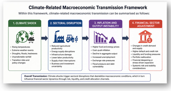
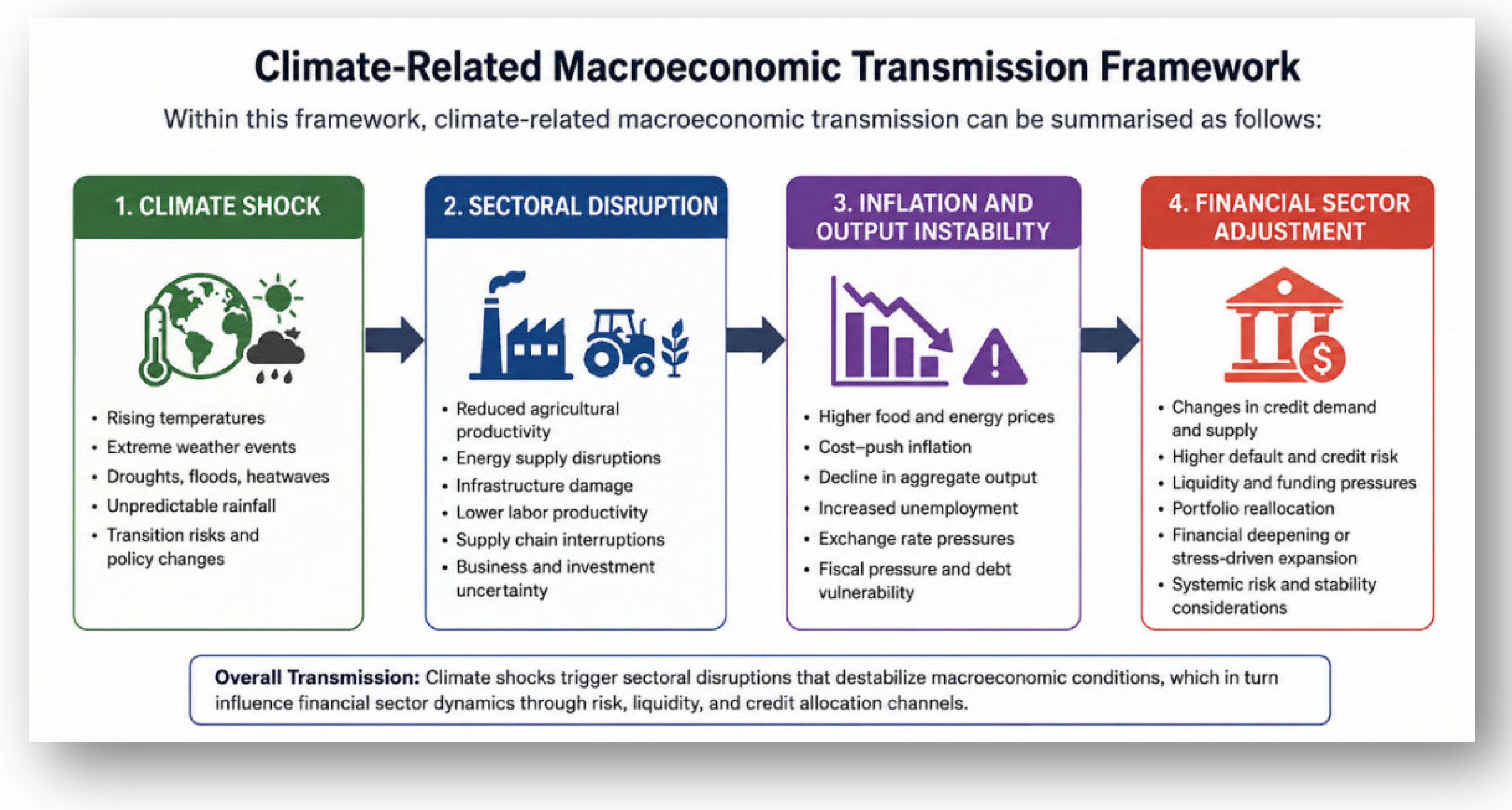
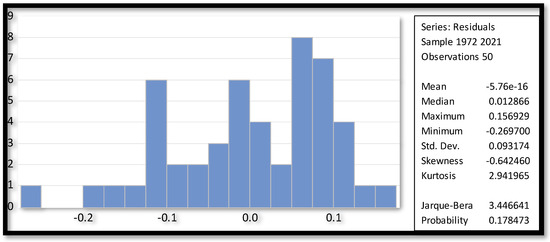
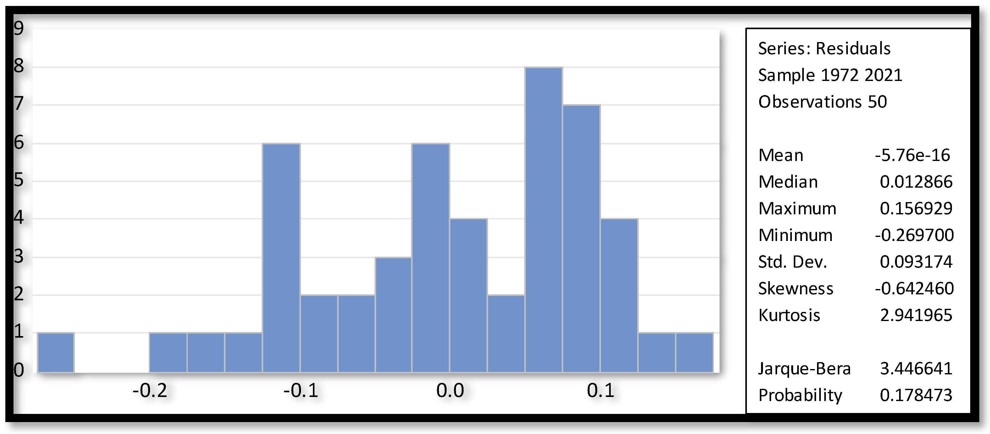
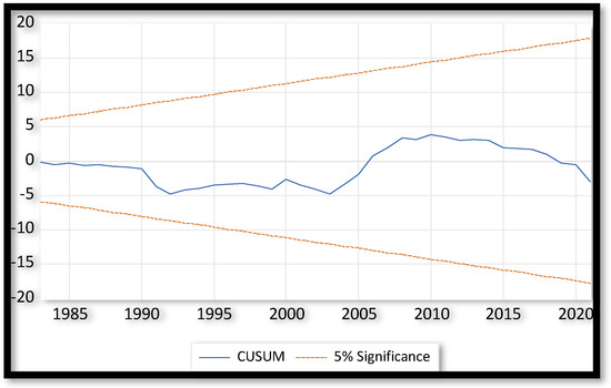
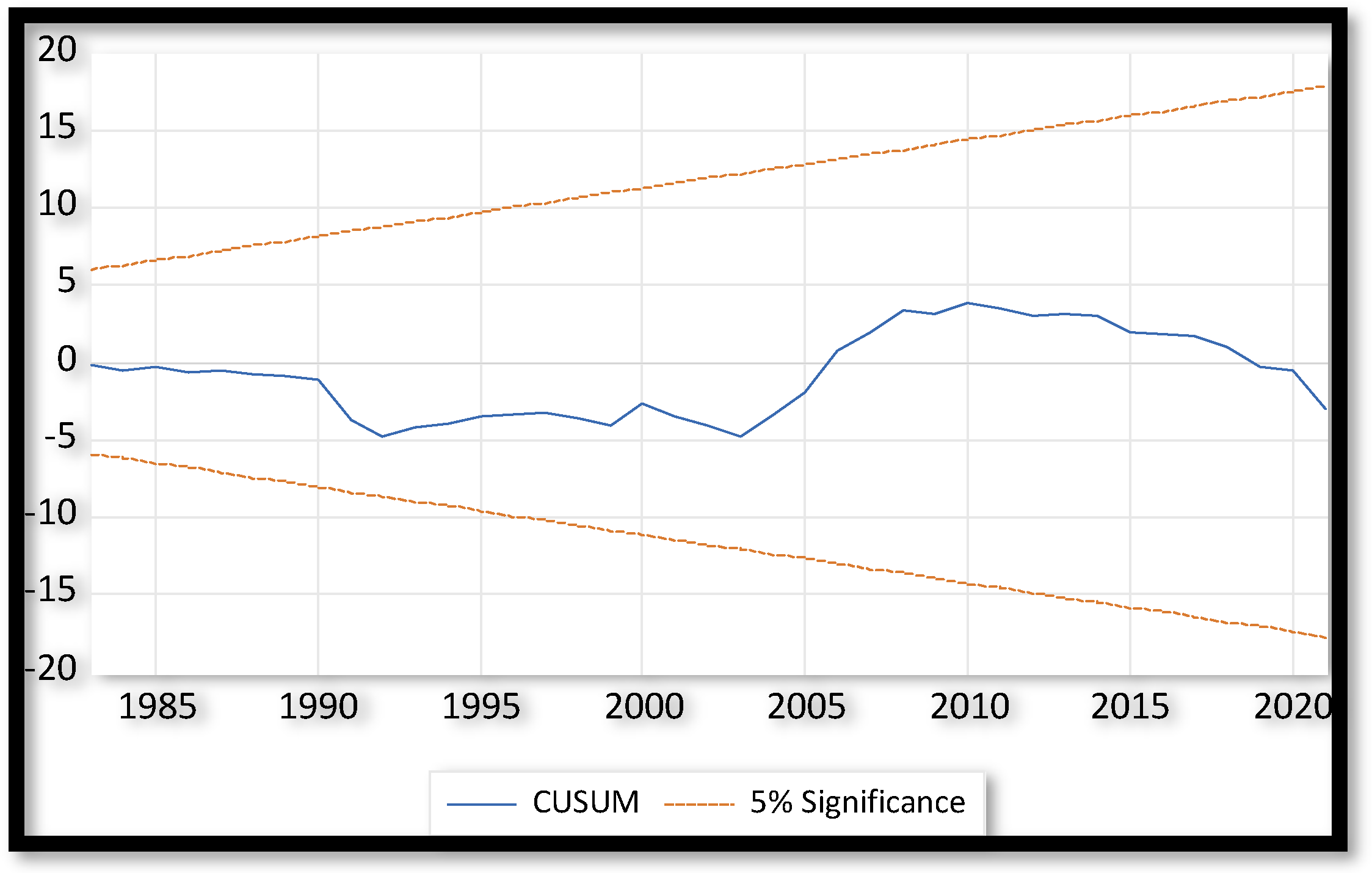

Disclaimer/Publisher’s Note: The statements, opinions and data contained in all publications are solely those of the individual author(s) and contributor(s) and not of MDPI and/or the editor(s). MDPI and/or the editor(s) disclaim responsibility for any injury to people or property resulting from any ideas, methods, instructions or products referred to in the content. |
© 2026 by the authors. Licensee MDPI, Basel, Switzerland. This article is an open access article distributed under the terms and conditions of the Creative Commons Attribution (CC BY) license.