


Abstract
The global energy transition has created a new financial ecosystem linking clean energy equities, transition metals, electric mobility firms, carbon allowances, and fossil energy assets. This study examines how shocks propagate within this ecosystem and whether geopolitical risk drives its tail co-movement by combining the Asymmetric Slope CAViaR model with Quantile VAR connectedness on daily data from March 2018 to May 2026. Under the standard Quantile VAR estimator, total connectedness rises from 46.6% at the median to 81.7% in the lower tail; however, a location-adjusted decomposition shows that most of this rise is mechanical, and model-free co-exceedance tests identify significant lower tail excess co-exceedances relative to Gaussian benchmarks, concentrated in the links between clean energy assets and the carbon and oil markets, although direct lower–upper tail differences are not statistically significant. The clean energy group generally acts as a net transmitter, whereas EU carbon allowances and Brent crude generally act as net receivers across the principal specifications; individual clean energy assets are not uniformly net transmitters in every specification. Contrary to our initial hypothesis, the daily geopolitical risk index is essentially disconnected from transition asset returns at every quantile. Connectedness jumped at the onset of COVID-19, while later geopolitical episodes left little imprint. These findings refine the diversification and hedging calculus for transition-themed portfolios.
Keywords:
energy transition; geopolitical risk; tail connectedness; clean energy equities; CAViaR; Quantile VAR; systemic risk JEL Classification:
G11; G15; Q42; Q54; C58
1. Introduction
The transition to a low-carbon economy has become one of the defining macro-financial forces of the present decade. As capital reallocates from fossil fuel incumbents toward renewable generation, electrified transport, and the critical minerals that underpin them, a distinct asset complex has emerged whose members clean energy equities, solar and wind funds, lithium and battery metal producers, electric vehicle manufacturers, and carbon emission allowances are increasingly held, traded, and risk-managed as a coherent thematic bloc (Yan & Cheung, 2025). Yet the systemic properties of this complex, and in particular the manner in which shocks propagate within it and between it and the fossil energy and geopolitical risk factors that surround it, remain insufficiently understood (Zhang et al., 2025; He, 2026; Luo et al., 2026). This gap is consequential: if the diversification that appears to separate clean energy and fossil assets in tranquil markets dissolves under stress, then the transition-aware portfolios now being assembled by institutional investors may be materially more fragile than conventional risk metrics suggest (El Khoury et al., 2025; Yan & Cheung, 2025).
This paper addresses that gap by mapping the tail-dependent connectedness of the transition risk complex. We assemble an eight-variable system spanning the clean energy equity, solar, wind, lithium and battery, electric mobility, EU carbon allowance, Brent crude, and geopolitical risk markets, observed daily from March 2018 to May 2026. To this system we apply a two-stage methodology that has proven well suited to capturing asymmetric, state-dependent dependence in financial networks: the Asymmetric Slope CAViaR model of Engle and Manganelli (2004) for the conditional tail risk dynamics of each series, coupled with the Quantile VAR connectedness framework of Diebold and Yilmaz (2012, 2014) and Ando et al. (2022) for the directional spillovers across the system at the median and at both distributional extremes.
Our analysis yields three principal results. First, connectedness in the transition risk complex is state-dependent, but less dramatically than conventional estimates suggest. Under the standard Quantile VAR estimator, the total connectedness index rises from 46.6% at the conditional median to 81.7% in the lower tail and 81.5% in the upper tail. A location-adjusted decomposition shows that most of this increase reflects the non-zero mean of extreme quantile residuals rather than genuine co-movement; model-free co-exceedance tests nonetheless show that joint lower tail events between the clean energy complex and the carbon and oil markets occur significantly more often than a Gaussian benchmark implies, although confidence intervals for the direct lower–upper tail differences include zero. Second, the integration is directional and economically interpretable. The clean energy complex acts predominantly as a net-transmitting group, while carbon allowances and Brent crude generally act as net receivers; we formalise this regularity as the Transition Risk Transmission Hypothesis (TRTH), and it is broadly supported across quantiles, covariance conventions, measures of geopolitical risk, and subsamples, without holding for every constituent asset in every specification. Third, and contrary to our priors, the daily geopolitical risk index is not a source of spillovers: it is essentially disconnected from transition asset returns at all quantiles, and its apparent net receiver role in the tails is an artefact of the location effect. Among transition-salient events, only the COVID-19 crash produced a large and statistically significant shift in connectedness.
This study contributes to three literatures. To the literature on energy transition finance, it provides a tail-focused, directional connectedness analysis of the transition risk complex that jointly covers clean energy equities, solar and wind funds, lithium and battery technology, electric mobility, carbon allowances, crude oil, and geopolitical risk. To the literature on systemic risk and financial networks, it shows that the tail amplification reported by standard Quantile VAR connectedness estimates can be largely mechanical, and it applies two simple diagnostics, a location-adjusted residual covariance and model-free co-exceedance tests, that separate genuine tail dependence from this artefact. To the literature on geopolitical risk in financial markets, it shows that, at daily frequency, the news-based geopolitical risk index does not transmit spillovers into the transition complex, which qualifies the view that geopolitical risk is a first-order driver of transition asset tail risk.
These contributions differ from existing quantile-connectedness research in three respects. First, prior studies typically analyse clean–dirty energy pairs (Saeed et al., 2021), climate policy uncertainty and renewables (Yan & Cheung, 2025), or carbon, green finance, and digital assets (Shojaei et al., 2026), whereas the present system places the critical mineral and electric mobility segments alongside carbon, oil, and geopolitical risk. Second, these studies generally report tail connectedness under a single residual covariance convention; we show that this convention drives much of the measured tail amplification and should be accompanied by diagnostics. Third, rather than treating univariate tail risk models and network measures as separate exercises, we link them by estimating a connectedness system on the CAViaR conditional quantile series themselves, in the spirit of White et al. (2015).
The remainder of the paper is organised as follows. Section 2 reviews the relevant literature. Section 3 develops the theoretical framework and hypotheses. Section 4 describes the data and methodology. Section 5 presents the empirical results. Section 6 reports robustness checks. Section 7 discusses the findings and their implications, and Section 8 concludes.
2. Literature Review
A substantial body of literature documents the financial behaviour of clean energy assets, with early contributions establishing that clean energy equities co-move with technology stocks and oil prices rather than with conventional utilities (Henriques & Sadorsky, 2008; Sadorsky, 2012). More recent work has examined the connectedness between clean energy and fossil energy markets, generally finding time-varying and crisis-sensitive linkages (Ferrer et al., 2018; Saeed et al., 2021). Related evidence from commodity and foreign exchange markets shows that spillover connectedness changes markedly during major economic and geopolitical crises, highlighting the state-dependent nature of cross-market shock transmission (Almansour et al., 2024). This study departs from the prevailing mean-based and bivariate focus by characterising the full multivariate, tail-dependent structure of the transition risk complex.
The measurement of geopolitical risk and its transmission to financial markets has advanced considerably since the construction of the Caldara and Iacoviello (2022) geopolitical risk index. A growing body of evidence links geopolitical shocks to elevated volatility and connectedness in energy and commodity markets (Antonakakis et al., 2017; Gong & Xu, 2022). Evidence from global equity markets similarly demonstrates that the structure and intensity of shock transmission change substantially across major financial and geopolitical crises (Shojaei et al., 2025). We contribute by positioning geopolitical risk explicitly within the transition complex and quantifying its directional role.
The connectedness framework of Diebold and Yilmaz (2012, 2014), and its quantile extension (Ando et al., 2022; Chatziantoniou et al., 2021), has become the standard apparatus for measuring directional spillovers in financial systems. Recent applications to carbon and green finance markets further demonstrate that connectedness structures and transmitter–receiver roles are state-dependent and can vary substantially across quantile regimes (Shojaei et al., 2026). The parallel literature on conditional tail risk modelling, anchored by the CAViaR approach of Engle and Manganelli (2004), provides the tools to characterise asymmetric downside dynamics. We bring these two strands together for the transition risk complex.
A critical reading of this literature reveals three limitations that motivate the present study. First, most connectedness studies of transition assets rely on mean-based spillover measures, which average across market states and may understate co-movement in crises (Antonakakis et al., 2017; Ferrer et al., 2018). Second, the quantile extensions that address this issue (Ando et al., 2022; Chatziantoniou et al., 2021) typically report large increases in tail connectedness without examining how much of the increase arises from the estimator itself. Exceedance-based evidence shows that cross-market correlations rise in bear markets but not in bull markets (Longin & Solnik, 2001), and dependence between oil and renewable energy stocks is asymmetric in the tails (Reboredo, 2015); a credible tail analysis should, therefore, distinguish genuine tail dependence from statistical artefacts. Third, the evidence on geopolitical risk and energy markets is mainly based on monthly data or event studies (Caldara & Iacoviello, 2022; Gong & Xu, 2022), leaving open whether the daily news-based index transmits shocks to transition assets, which are priced continuously.
Despite the rapid growth of transition finance, few studies characterise the directional, tail-dependent connectedness of the clean energy, transition metal, electric mobility, carbon, fossil energy, and geopolitical risk markets within a single system, and none, to our knowledge, examines how sensitive the resulting tail estimates are to the estimator. The present paper addresses this gap and, in doing so, tests a falsifiable hypothesis, the TRTH, concerning the structure of transition risk transmission.
3. Theoretical Framework and Hypothesis Development
3.1. A Transition Risk Transmission Framework
We conceptualise the transition risk complex as a network in which shocks propagate through three economic channels. The first is a real options channel: clean energy and transition metal valuations are dominated by the present value of distant growth options, rendering them highly sensitive to discount rate and sentiment shocks that, in stressed states, are common across the complex. The second is a funding liquidity channel (Brunnermeier & Pedersen, 2009): leveraged thematic positions in clean energy and battery metal assets transmit funding shocks across the system when collateral values fall. The third is a policy and geopolitical uncertainty channel: because transition assets are unusually exposed to policy and geopolitical developments, shocks to the geopolitical risk factor propagate disproportionately into the complex.
These channels have established theoretical foundations. The real options channel follows from models in which firms whose value is dominated by growth options carry higher and more time-varying systematic risk (Berk et al., 1999); in a sustainable-investing equilibrium, green assets also carry exposure to shifts in climate concerns that are common across the green segment (Pástor et al., 2021). The funding liquidity channel follows from Brunnermeier and Pedersen (2009) and from wealth effect models of contagion, in which losses on one leveraged position force portfolio-wide deleveraging (Kyle & Xiong, 2001); thematic funds that hold overlapping baskets of clean energy, battery, and electric vehicle stocks are a natural conduit for this mechanism. The policy uncertainty channel follows from Pástor and Veronesi (2012) and Kelly et al. (2016), who show that uncertainty about government policy is priced and raises co-movement; transition assets, whose cash flows depend on subsidies, mandates, and carbon prices, are particularly exposed, and the pricing of carbon risk links them to the carbon market (Bolton & Kacperczyk, 2021). Oil and carbon futures, by contrast, are driven mainly by their own supply and demand fundamentals and regulatory calendars and are linked to equity markets through index investment flows (Tang & Xiong, 2012); this asymmetry motivates the expectation that equity-based transition assets transmit, and commodity-based assets receive, shocks. Throughout, connectedness measures capture predictive spillovers in the forecast error variance decomposition rather than structural causality, so the hypotheses below are statements about the direction of predictive transmission.
3.2. Hypotheses
These channels jointly imply a state-dependent and directional connectedness structure, which we formalise in three testable hypotheses as follows:
H1.
Total connectedness in the transition risk complex is significantly higher in the tails than at the median.
H2.
The clean energy complex is a net transmitter of tail risk, whereas fossil energy and carbon allowances are net receivers; the Transition Risk Transmission Hypothesis.
H3.
The geopolitical risk factor is the single largest net transmitter of lower tail spillovers within the system.
4. Data and Methodology
4.1. Data and Variable Construction
The empirical analysis employs daily data on eight system variables observed from 16 March 2018 to 29 May 2026, yielding 2044 daily return observations after alignment. The start date is the first date on which all series are available, since the electric vehicle index begins on 15 March 2018. The variables are: (i) CLEANEQ, the S&P Global Clean Energy Index; (ii) SOLARETF, the Invesco Solar ETF (TAN); (iii) WINDETF, the First Trust Global Wind Energy ETF (FAN); (iv) LITHIUM, the Global X Lithium & Battery Tech ETF (LIT); (v) EVMOBIL, the Solactive Autonomous & Electric Vehicles Index; (vi) CARBONEU, ICE EU carbon allowance (EUA) futures; (vii) BRENTOIL, ICE Brent crude oil futures; and (viii) GEOPOL, the daily Caldara–Iacoviello geopolitical risk index (GPRD). Daily closing prices of the seven market series (continuous benchmark contracts for the two futures) were obtained from Investing.com, and GEOPOL from the website of Matteo Iacoviello (Caldara & Iacoviello, 2022). Table 1 defines each variable and gives its source. Because GEOPOL is published for every calendar day while the market series follow exchange calendars, the eight series are aligned on the dates on which all markets traded. All series are transformed into continuously compounded daily changes, rt = 100 × ln(Pt/Pt−1). The sample spans several transition-salient episodes, including the COVID-19 crash (March 2020), the green stimulus rally (late 2020–2021), the Russia–Ukraine invasion and ensuing energy crisis (2022), and subsequent geopolitical escalations through 2024–2025.
Table 1.
Variable definitions and data sources.
Two features of GEOPOL deserve comment. First, the index measures the share of articles discussing adverse geopolitical events in ten leading newspapers published in the United States, the United Kingdom, and Canada (Caldara & Iacoviello, 2022). It, therefore, captures geopolitical risk as perceived through English language, predominantly Western media, which may differ from how conditions are perceived elsewhere; this news-based construction is shared by other text-based uncertainty indices (Baker et al., 2016). Because a broader, multi-language daily index is not publicly available, we assess the sensitivity of the results to the measurement of GEOPOL using its acts and threats sub-indices and its seven-day moving average (Section 6) and discuss this limitation in Section 7.3. Second, we use the log change in the index rather than its level. GEOPOL is a ratio of article counts, so its log change measures the proportional change in geopolitical news intensity; this places it on the same scale-free, percentage basis as the return series and corresponds to the notion of a geopolitical shock (innovation) in a connectedness system. The daily log level is persistent (first-order autocorrelation 0.60 over the sample), whereas the log change is strongly mean-reverting (first-order autocorrelation −0.45), as expected for a noisy count-based measure. Because the log change is not the only defensible transformation, Section 6 also reports results with GEOPOL in log levels.
Summary statistics are reported in Table 2. All series exhibit excess kurtosis and highly significant Jarque–Bera statistics, and the Elliott–Rothenberg–Stock (ERS) DF-GLS test rejects the unit root null for every series at the 1% level (Elliott et al., 1996), validating the subsequent vector autoregressive analysis.
Table 2.
Descriptive statistics of daily return series (March 2018–May 2026).
4.2. The Asymmetric Slope CAViaR Model
To capture the conditional tail dynamics of each series, we estimate the Asymmetric Slope CAViaR model of Engle and Manganelli (2004). The conditional quantile of returns evolves as:
where β1 governs the persistence of the conditional quantile and the ratio β3/β2 measures the asymmetry of the response to negative versus positive shocks. Because the conditional 5% quantile of returns is negative, we follow Engle and Manganelli (2004) and report the coefficients for the (positive) VaR, so that positive β2 and β3 indicate that positive and negative shocks, respectively, raise tail risk. The model is estimated by minimising the regression quantile (tick) loss (Koenker & Bassett, 1978), starting from 2000 randomly drawn initial values and refining the best fifteen with Nelder–Mead and Powell searches. Standard errors follow the asymptotic formula of Engle and Manganelli (2004) with a kernel estimate of the density at the quantile, and specification adequacy is assessed with the Dynamic Quantile (DQ) test, using a constant, four lagged hits and the current VaR as instruments.
VaRt(q) = β0 + β1 VaRt−1(q) + β2 max(rt−1, 0) + β3 max(−rt−1, 0)
The two stages are linked as follows. The QVAR system is estimated on the return series themselves, so the CAViaR estimates do not enter the QVAR as regressors. CAViaR plays two roles. First, it provides a univariate diagnostic of the tail behaviour of each series, its persistence and asymmetry, which motivates studying connectedness at extreme quantiles rather than at the mean. Second, the fitted conditional VaR series are themselves used as the inputs of a tail risk connectedness system: we estimate a VAR on the daily log changes of the eight CAViaR VaR series and compute the same generalised forecast error variance decomposition measures. This captures how shocks to the tail risk of one market predict changes in the tail risk of the others (White et al., 2015). Section 6 compares this CAViaR-based network with the QVAR network.
4.3. Quantile VAR Connectedness
Directional spillovers are measured using the connectedness framework of Diebold and Yilmaz (2012, 2014), estimated within a Quantile VAR specification (Ando et al., 2022; Chatziantoniou et al., 2021) that permits the dependence structure to differ across quantiles. For each quantile τ, each equation of the system yt = c(τ) + B1(τ)yt−1 + … + Bp(τ)yt−p + ut(τ) is estimated by linear quantile regression, and the residual covariance matrix Σ(τ) is computed from the quantile residuals. Each row of the H-step generalised forecast error variance decomposition (GFEVD; Pesaran & Shin, 1998) is normalised to sum to 100. For each variable i, we compute the directional connectedness TO and FROM all other variables, the NET connectedness (NETi = TOi − FROMi), and the total connectedness index TCI = (1/N)ΣiFROMi. Because every off-diagonal element enters exactly one TO and one FROM total, ΣiNETi = 0 holds as an identity, which provides a numerical check on the estimates. A positive NETi identifies variable i as a net transmitter of shocks; a negative value identifies a net receiver. These are measures of predictive spillover in forecast error variance and should not be read as evidence of causality. The system is estimated with lag order p = 1 (selected by the Bayesian information criterion), forecast horizon H = 10, and evaluated at q ∈ {0.05, 0.50, 0.95}.
Two implementation choices deserve attention. First, following the standard convention (Chatziantoniou et al., 2021), Σ(τ) is computed as the raw second-moment matrix of the quantile residuals. At extreme quantiles, these residuals have non-zero means by construction, so their raw second moments contain a component, the product of the residual means, that is present even for independent variables. We, therefore, also report a location-adjusted (centred) version, in which Σ(τ) is the covariance matrix of the quantile residuals, and we complement the model-based measures with model-free lower and upper tail co-exceedance rates compared against a Gaussian benchmark (Longin & Solnik, 2001). Second, statistical uncertainty in the static measures is assessed with a moving block bootstrap (Künsch, 1989) with block length 20 and 199 replications, from which percentile 95% confidence intervals for the TCI and each NET are obtained. Time-varying dynamics are tracked through a 200-day rolling window. Regime shifts in the rolling TCI are identified with the Bai and Perron (1998, 2003) procedure for multiple shifts in mean, using 15% trimming, a maximum of five breaks, and sequential sup-F(l + 1|l) tests with a Bartlett heteroskedasticity and autocorrelation consistent (HAC) variance and the critical values of Bai and Perron (2003). The response to specific events is assessed by comparing the mean TCI in the 20 trading days before and after each event date with a HAC t-test.
5. Empirical Results
5.1. Price Dynamics and Preliminary Analysis
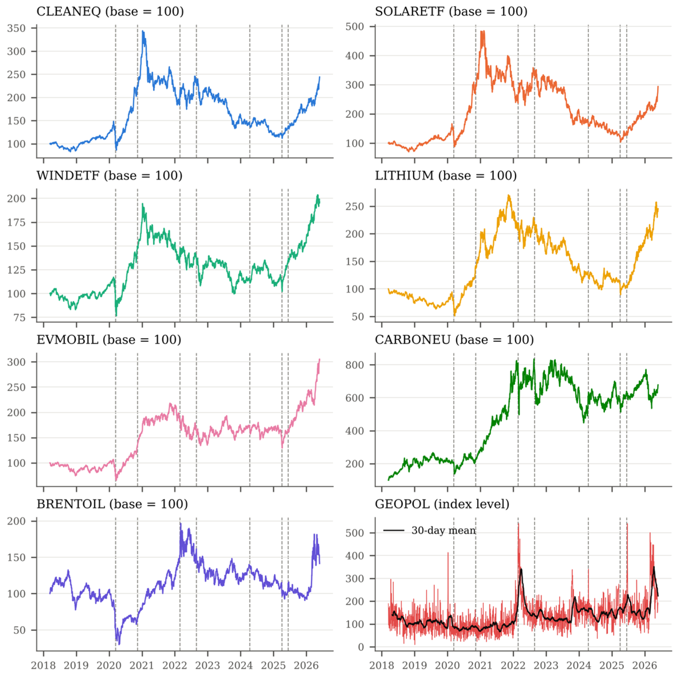
Figure 1 plots the price dynamics of the eight system variables over the sample period, with vertical markers denoting the major transition-salient events. The clean energy series shares the pronounced 2020–2021 rally, which peaked in early 2021, and the subsequent retracement that characterised the post-pandemic transition cycle. The carbon allowance price rose strongly to a peak in August 2022, and Brent shows its sharpest movements in the April 2020 collapse and the March 2022 spike. The geopolitical risk index is far noisier than any market series at daily frequency, with its largest values at the start of the Russian invasion of Ukraine (February–March 2022), during the June 2025 Israel–Iran war and in early March 2026. The co-movement of the clean energy series and their divergence from the carbon, oil and geopolitical risk series provide initial motivation for the connectedness analysis that follows.
Figure 1.
Price dynamics of all system variables (March 2018–May 2026). Note: Market variables are rebased to 100 on 15 March 2018; GEOPOL is shown in index levels with its 30-day moving average. Vertical dashed lines mark the COVID-19 crash (11 March 2020), the green stimulus rally (9 November 2020), the Russia–Ukraine invasion (24 February 2022), the global energy crisis peak (26 August 2022), the Iran–Israel escalation (13 April 2024), the US tariff shock (2 April 2025), and the Israel–Iran war (13 June 2025).
5.2. Descriptive Statistics
Table 2 reports the descriptive statistics. Measured by the standard deviation of daily changes, GEOPOL is by far the most volatile series (43.15), reflecting the noisiness of daily news counts, followed by Brent crude (2.66), carbon allowances (2.65), and the solar ETF (2.57); the wind ETF is the least volatile (1.41). All series are negatively skewed, and Brent displays the largest excess kurtosis (16.46), driven by the April 2020 collapse in oil prices. All series depart significantly from normality according to the Jarque–Bera test; the ERS test rejects a unit root for every series, and the Ljung–Box statistics on squared changes indicate strong volatility clustering.
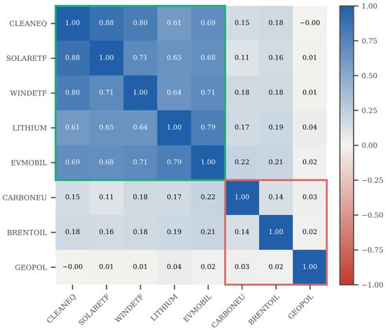
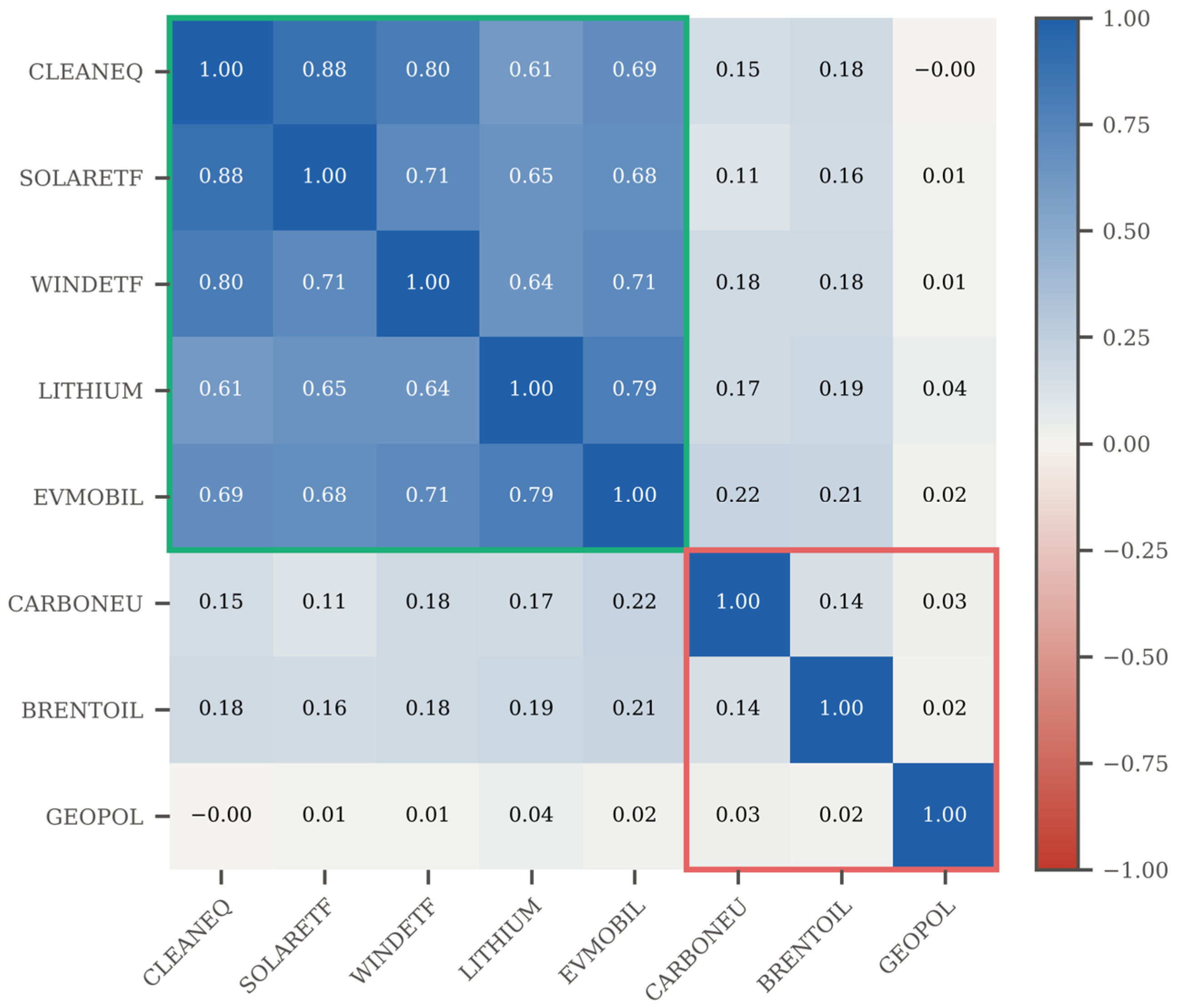
The unconditional pairwise correlation matrix is displayed in Figure 2. A clear block pattern is visible: the clean energy cluster (CLEANEQ, SOLARETF, WINDETF, LITHIUM, EVMOBIL) is highly correlated within itself (pairwise correlations between 0.61 and 0.88) but only weakly correlated with carbon allowances and Brent crude (between 0.11 and 0.22), and GEOPOL is essentially uncorrelated with every market variable (|ρ| ≤ 0.04). This unconditional clustering serves as the benchmark against which the conditional, quantile-specific structure is evaluated below.
Figure 2.
Unconditional pairwise correlation matrix (full sample: March 2018–May 2026). Note: Pairwise Pearson correlations of daily changes. The green box demarcates the clean energy complex; the red box demarcates the carbon, oil, and geopolitical risk block. Blue denotes positive and red negative correlation.
5.3. Conditional Tail Risk Dynamics
Table 3 reports the Asymmetric Slope CAViaR estimates at the 5% quantile. The persistence parameter β1 lies between 0.81 and 0.94 and is significant at the 1% level for all series, confirming the strong autocorrelation of conditional tail risk. For all seven market series, β3 exceeds β2, so a negative return raises next-day VaR by more than a positive return of the same size; the asymmetry ratio β3/β2 ranges from 1.11 (CARBONEU) to 4.08 (WINDETF). β3 is significant at least at the 10% level for every market series, whereas β2 is significant at the 5% level only for CLEANEQ, SOLARETF, and LITHIUM. GEOPOL behaves differently: a rise in geopolitical news intensity raises its VaR (β2 > 0), while a fall lowers it (β3 < 0), so its asymmetry ratio is negative. This reflects the strong mean reversion of daily news counts rather than leverage-type asymmetry, and the GEOPOL ratio should not be compared with those of the market series. The empirical hit rates lie within 0.06 percentage points of the nominal 5%, and the DQ test does not reject correct specification at the 5% level for any series.
Table 3.
CAViaR asymmetric slope parameter estimates (q = 0.05).
5.4. Static Connectedness Across Quantiles
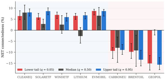
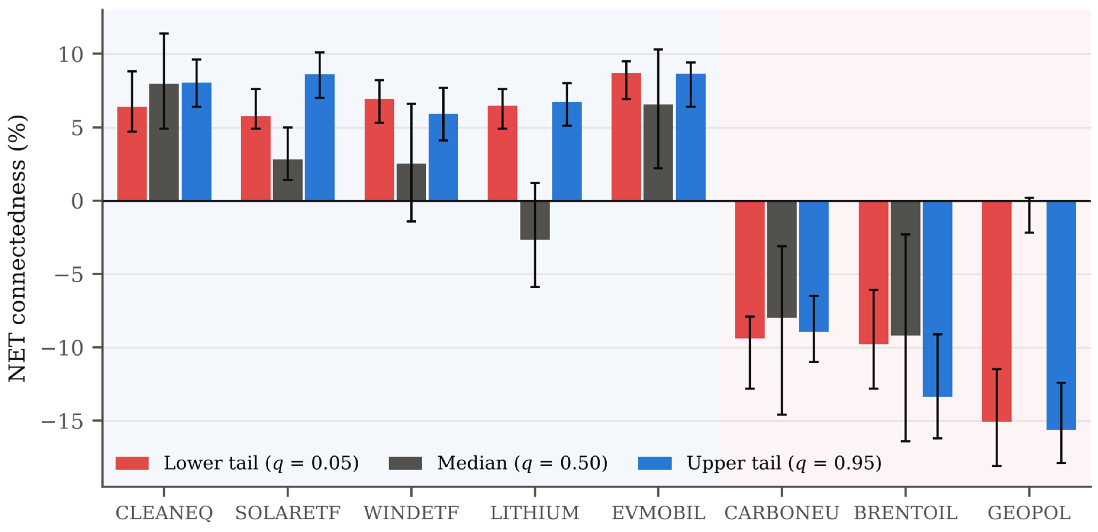
Table 4 reports the static connectedness matrices for the lower (q = 0.05), median (q = 0.50), and upper (q = 0.95) quantiles, estimated over the full sample; within each panel the NET values sum to zero, as the methodology requires. Under the standard estimator, total connectedness rises from 46.6% at the median to 81.7% in the lower tail and 81.5% in the upper tail, and the bootstrap confidence intervals of the tail TCIs lie entirely above that of the median TCI, which is consistent with Hypothesis H1. The NET row captures directionality. All five clean energy series are net transmitters in both tails (NET between 5.8 and 8.7), while CARBONEU (−9.4 and −8.9) and BRENTOIL (−9.8 and −13.4) are net receivers in the lower and upper tails, as predicted by Hypothesis H2; the bootstrap intervals exclude zero for every market variable in both tails. At the median, CLEANEQ, SOLARETF, WINDETF, and EVMOBIL remain net transmitters, LITHIUM becomes a small net receiver (−2.6), and CARBONEU and BRENTOIL remain net receivers, although at the median the bootstrap intervals for WINDETF and LITHIUM include zero. Hypothesis H3 is not supported: GEOPOL is not a net transmitter at any quantile. At the median, it is almost completely disconnected from the system, receiving 0.35% of its forecast error variance from the other variables and contributing 0.28% to them, whereas in the tails, it appears as the largest net receiver (−15.1 and −15.7). Section 6 shows that this tail result, like much of the rise in the tail TCI, is an artefact of the location component of Σ(τ).
Table 4.
Quantile connectedness matrices at q = 0.05, q = 0.50, and q = 0.95.
Figure 3 displays the NET directional connectedness of all variables across the three quantiles, with bootstrap 95% confidence intervals, confirming the transmitter–receiver partition between the clean energy complex and the carbon and oil markets.
Figure 3.
NET directional connectedness across all variables and quantile regimes (with bootstrap 95% confidence intervals). Note: Bars show NET connectedness (TO − FROM, %) at each quantile under the standard estimator; whiskers are moving block bootstrap 95% confidence intervals. Values above zero indicate net transmitters and values below zero net receivers. The blue shaded area marks the clean energy complex; the red shaded area marks the carbon, oil, and geopolitical risk block.
5.5. Time-Varying Connectedness and Event Transmission
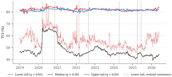
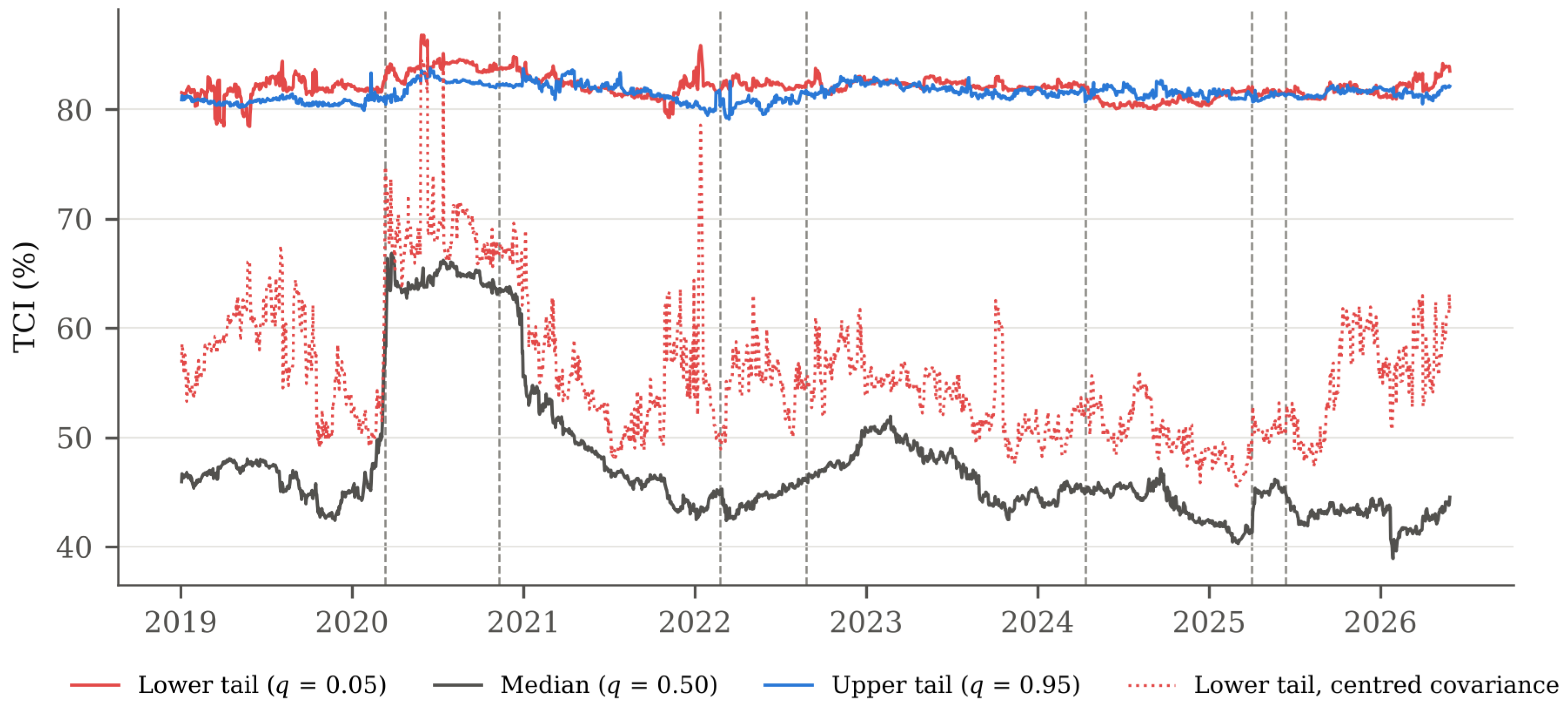
Figure 4 shows the time-varying total connectedness index at the three quantiles. Under the standard estimator, the tail indices move in a narrow band (lower tail: 78.4–86.8%) well above the median index, which varies much more (38.9–66.8%). The median index shows the clearest response to transition-salient events: it jumps at the onset of the COVID-19 crisis in March 2020 and remains elevated until spring 2021 before falling back. The location-adjusted lower tail index (dotted line) lies between the two (mean 56.0%, against 47.7% for the median index and 82.1% for the standard lower tail index) and co-moves with the median index (correlation 0.74), but it is far more volatile. This volatility reflects the imprecision of 5% quantile regressions estimated on 200 observations, of which only about ten lie in the tail; conversely, the apparent stability of the standard tail index is largely a product of the mechanical location component. We, therefore, base inference about tail connectedness on the full-sample estimates and treat the rolling tail indices as descriptive.
Figure 4.
Time-varying total connectedness index across quantile regimes (200-day rolling window, 2019–2026). Note: TCI estimated over 200-day rolling windows at q = 0.05, 0.50, and 0.95 with the standard estimator; the dotted line is the lower tail TCI computed with the location-adjusted (centred) residual covariance. The first estimate is dated at the end of the first 200-day window (January 2019). Vertical dashed lines mark the events listed under Figure 1.
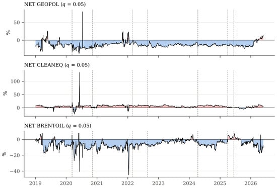
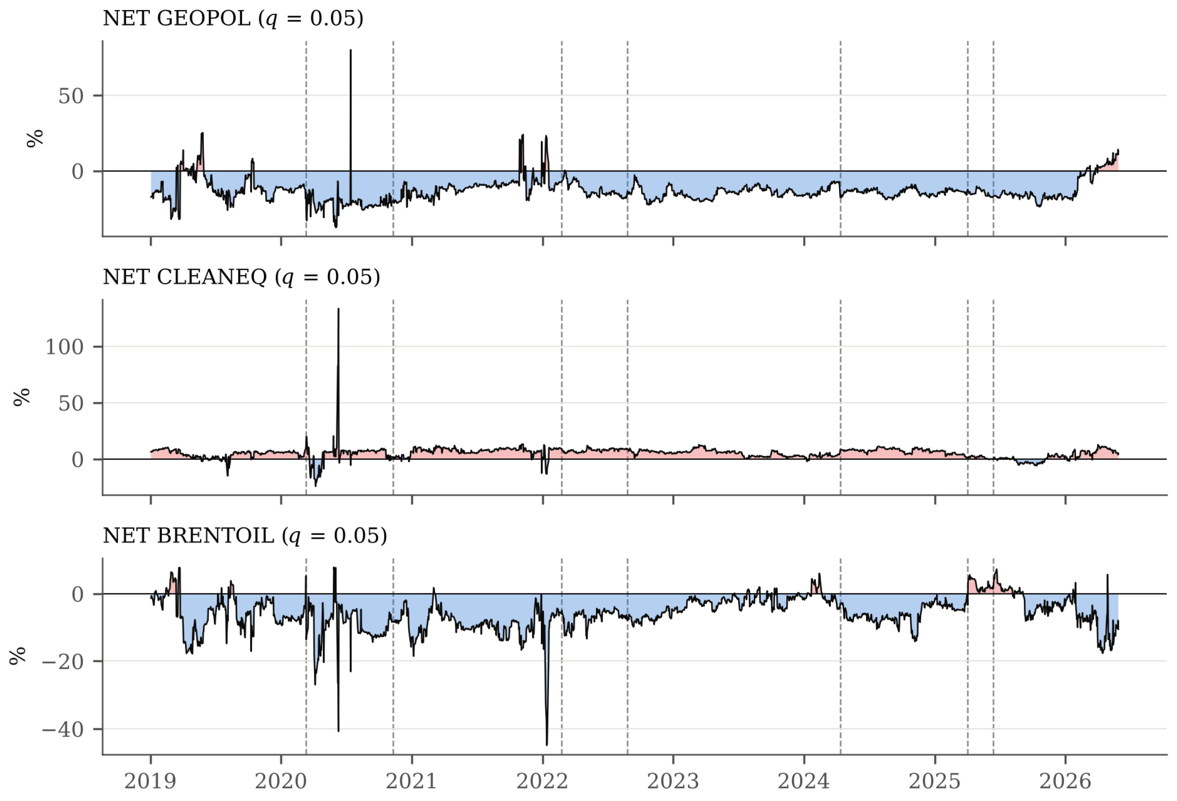
Figure 5 decomposes the network dynamics through the rolling lower tail NET connectedness of GEOPOL, CLEANEQ, and BRENTOIL. Under the standard estimator, GEOPOL is a net receiver in 94% of the rolling windows, CLEANEQ is a net transmitter in 92%, and BRENTOIL is a net receiver in 90%. The same qualitative pattern holds with the centred covariance, although those rolling estimates are noisy: GEOPOL is a net transmitter in only 16% of the windows, CLEANEQ is a net transmitter in 78%, and BRENTOIL is a net receiver in 85%. At no point, including the months after the 2022 invasion of Ukraine, does GEOPOL become a persistent net transmitter.
Figure 5.
Time-varying NET directional connectedness of GEOPOL, CLEANEQ, and BRENTOIL (q = 0.05). Note: Rolling NET connectedness (200-day window) at the 5% quantile under the standard estimator; red shading marks net transmitter and blue shading net receiver episodes. Vertical dashed lines mark the events listed under Figure 1.
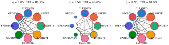
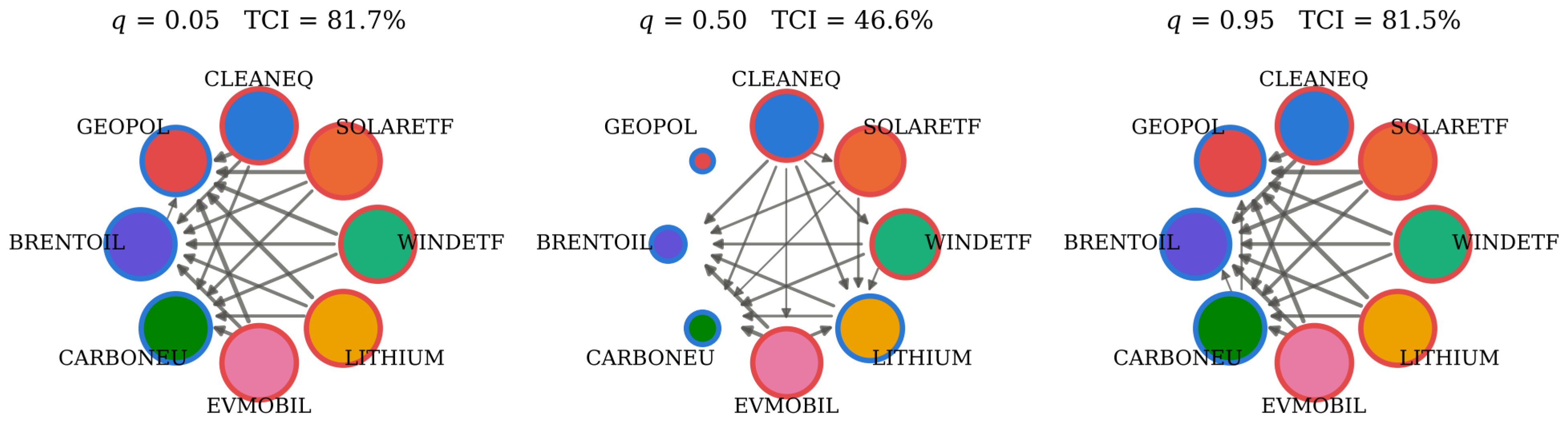
Figure 6 presents the connectedness network in topological form at the three quantiles, with arrows showing net pairwise spillovers. In all three panels, the dominant arrows run from the clean energy nodes towards CARBONEU and BRENTOIL. At the median, GEOPOL is an isolated node. In the tails, all nodes become larger, and GEOPOL receives arrows from every market node; as shown in Section 6, this tail pattern is driven by the location component of Σ(τ) rather than by genuine dependence.
Figure 6.
Quantile connectedness network topology at q = 0.05, q = 0.50, and q = 0.95. Note: Node colour identifies the variable; node size is proportional to total (TO + FROM) connectedness; red borders denote net transmitters and blue borders net receivers. Arrows show net pairwise directional spillovers (θji − θij) above 0.5 percentage points, with width proportional to their size. All panels use the same circular layout; the TCI is reported above each panel.
6. Robustness Checks
We subject the principal findings to four sets of robustness checks: specification sensitivity, structural breaks and event effects, expanding window stability, and alternative measures of tail dependence. Table 5 reports the specification sensitivity results. Panel A varies the forecast horizon (H = 5, 15, 20), the lag order (p = 2), the variance-decomposition scheme (Cholesky with the baseline and the reverse ordering), and the quantile (q = 0.01, 0.10, 0.90, 0.99). The TCI and NET measures are virtually invariant to the horizon and the lag order because the estimated lag coefficients are small and the decomposition is dominated by the contemporaneous covariance. Tail connectedness increases as the quantile moves further into the tails (77.4% at q = 0.10 and 85.5% at q = 0.01). The Cholesky decomposition yields a lower TCI, and its NET measures are dominated by whichever variable is ordered first, which illustrates why the order-invariant generalised decomposition is used as the baseline. Panel B varies the measurement of geopolitical risk and the composition of the system. Replacing GPRD with its acts or threats sub-index or with its seven-day moving average, or entering it in log levels, leaves the TCI and the clean energy transmitter/carbon and oil receiver partition unchanged, and GEOPOL is never a net transmitter (its lower tail NET ranges from −17.6 to −11.6, and its median NET from −1.9 to −0.1). Dropping CARBONEU, the only regionally bound variable, or dropping GEOPOL altogether also leaves the partition intact. Panel C shows that the averages of the rolling window estimates are insensitive to the window length.
Table 5.
Sensitivity of TCI and NET connectedness to specification choices.
Table 6 reports Bai–Perron tests applied to the rolling TCI series (Panel A) and event window tests (Panel B). For the lower tail index, the sequential procedure selects four breaks, but the regime means differ by at most 2.7 percentage points (81.0–83.7%), so standard tail connectedness is statistically but not economically unstable. The median index displays economically larger shifts: it rises from 46.0% to 61.2% at the break dated 06 March 2020, at the onset of the COVID-19 crisis, falls back to 45.5% after April 2021, and settles at 42.9% in the final regime. The event window tests in Panel B confirm that the COVID-19 crash produced by far the largest increase (+14.5 percentage points at the median). The April 2025 US tariff shock raised median connectedness by 3.4 points, whereas the Russia–Ukraine invasion (−1.1) and the later geopolitical episodes produced small or negative changes. These results do not support the view that geopolitical events are the main drivers of shifts in transition risk connectedness. Because rolling window estimates adjust gradually and overlap heavily, the event window tests should be read as descriptive.
Table 6.
Structural breaks and event effects in the rolling TCI series.
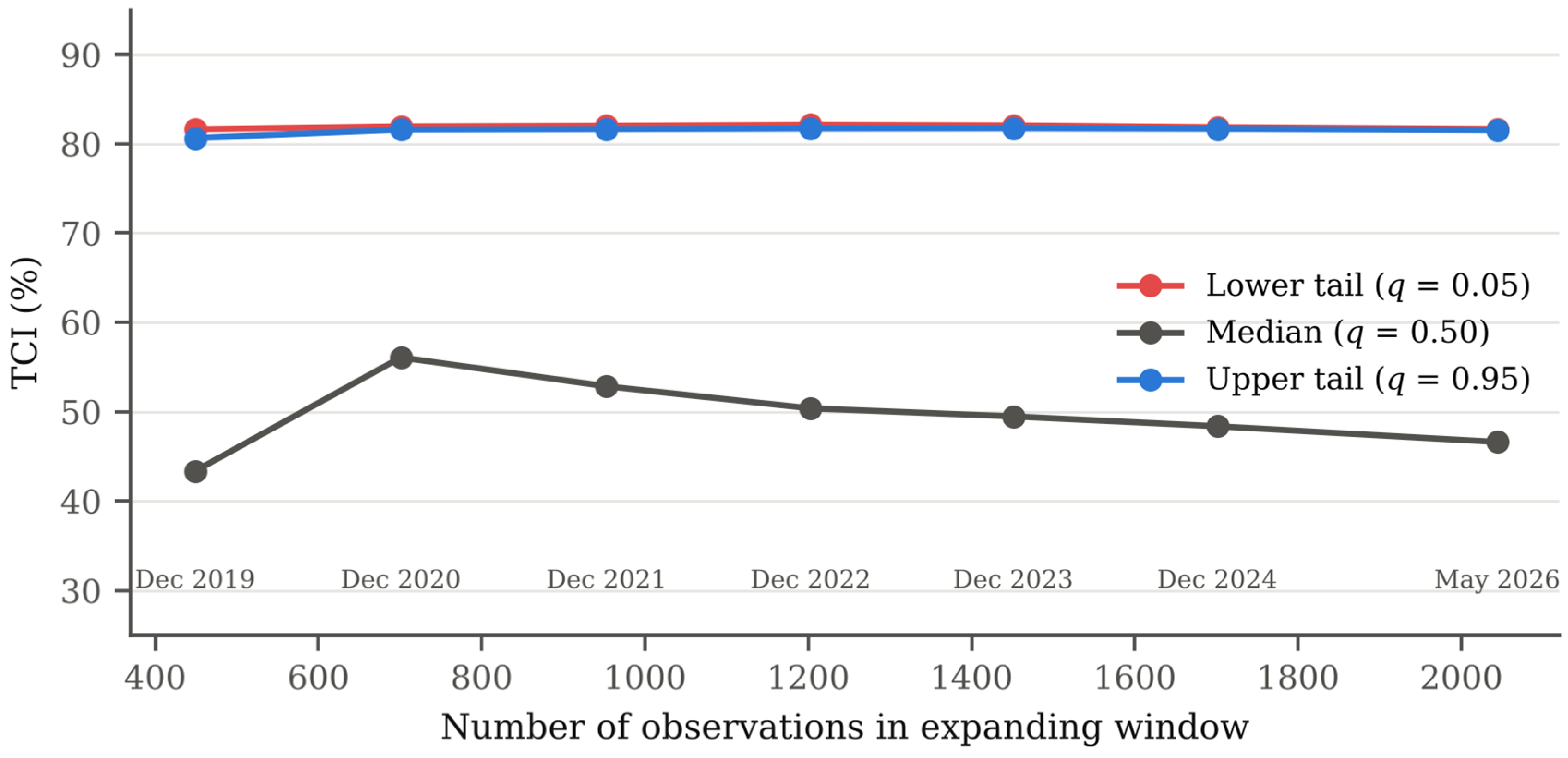
Table 7 reports the expanding window analysis, which is also displayed in Figure A1 (Appendix A). As the sample is extended from December 2019 through May 2026, the lower tail TCI stays between 81.6% and 82.1% and the transmitter–receiver partition holds in every window. The median TCI is more sensitive to the sample: it rises from 43.4% to 56.1% once 2020 is included and then declines gradually to 46.6%, mirroring the COVID-19 regime identified in Table 6. The principal results are, therefore, not an artefact of a particular subsample.
Table 7.
Total connectedness index across expanding windows.
Finally, we examine whether the tail amplification and the role of GEOPOL survive alternative measures of tail dependence. Table 8 reports the QVAR measures computed with the location-adjusted (centred) residual covariance and the connectedness of the CAViaR VaR series. With the centred covariance, the TCI is 47.4% in the lower tail, 46.6% at the median, and 47.2% in the upper tail. The bootstrap 95% interval for the lower tail minus median difference is [0.31, 3.00] percentage points, against [29.84, 38.79] under the standard estimator. A small but statistically significant amplification, therefore, remains, but most of the tail amplification in Table 4 reflects the non-zero mean of extreme quantile residuals. This component inflates the cross-moments of all pairs, including pairs of independent variables, which is why GEOPOL, uncorrelated with every market series, appears strongly connected in the tails. With the centred covariance, GEOPOL’s NET is close to zero at every quantile (−0.41, −0.07, −1.63), while CLEANEQ and EVMOBIL remain the largest transmitters and CARBONEU and BRENTOIL remain net receivers. The CAViaR-based network (VAR(1) on the log changes of the VaR series) tells the same story: tail risk shocks are shared within the clean energy complex (TCI 35.9%), CLEANEQ is the largest transmitter of tail risk (NET 6.88), and the tail risk of CARBONEU, BRENTOIL, and GEOPOL is almost entirely idiosyncratic (own shares of 97.4%, 92.1%, and 99.5%).
Table 8.
Location-adjusted QVAR and CAViaR-based tail risk connectedness.
Because the model-based measures depend on how Σ(τ) is estimated, Table 9 also reports model-free co-exceedance rates: the probability that variable j falls in its own 5% tail given that variable i does, averaged across pairs, compared with the rate implied by a bivariate Gaussian distribution with the same correlation. Lower tail co-exceedances exceed the Gaussian benchmark within the clean energy complex (0.463 against 0.414), between the clean energy complex and the carbon and oil markets (0.159 against 0.097) and between carbon and oil (0.147 against 0.085), and the bootstrap intervals for these differences exclude zero. Upper tail co-exceedances, by contrast, are not significantly different from the Gaussian benchmark, and GEOPOL shows no tail dependence with the market variables in either tail. The evidence, therefore, indicates modest excess lower tail co-exceedance relative to Gaussian benchmarks, particularly between clean energy assets and carbon and oil. However, the 95% confidence intervals for all direct lower minus upper differences in Table 9 include zero; consequently, a statistically significant asymmetry between the two tails is not established. H1 receives qualified support for tail dependence relative to the median or Gaussian benchmarks, but not for a statistically significant lower–upper asymmetry.
Table 9.
Model-free tail co-exceedance rates (5% tails).
7. Discussion and Implications
7.1. Interpretation of the Main Findings
The evidence supports H2, qualifies H1, and rejects H3. The clean energy transmitter/carbon and oil receiver partition (H2) is most consistent at the group level: the clean energy group predominantly transmits net spillovers across quantiles and the main robustness checks, whereas individual assets do not always retain positive NET values or statistically significant transmitter status in every specification. The group-level pattern is present in 85% of the 200-day rolling windows at the lower tail and median (96% at the upper tail). The only exception among the static checks is the Cholesky decomposition with reverse ordering, which by construction assigns the common contemporaneous component to the first-ordered variables. This partition is consistent with the real options and funding liquidity channels of our framework: equity-based transition assets, whose valuations are dominated by long-dated growth options and which are held in overlapping thematic portfolios, transmit discount rate and sentiment shocks, which the commodity-based carbon and oil markets, driven mainly by their own fundamentals, absorb. Regarding H1, the large rise in connectedness from the median to the tails produced by the standard QVAR estimator is mostly mechanical; the model-free co-exceedance evidence nonetheless shows that joint lower tail events between the clean energy complex and the carbon and oil markets are significantly more frequent than a Gaussian model implies, indicating modest lower tail dependence beyond the Gaussian benchmark but not a statistically established lower–upper tail asymmetry because the corresponding difference intervals include zero. Regarding H3, the daily geopolitical risk index neither transmits nor receives meaningful spillovers. A plausible interpretation is that geopolitical news affects transition assets mainly through slower-moving channels, such as energy security policy and supply chain reorganisation, that are not captured by day-to-day changes in news intensity, and that daily news counts contain substantial noise. The policy and geopolitical uncertainty channel may, therefore, operate at lower frequencies than those examined here.
7.2. Implications for Investors and Policymakers
For investors, three specific implications follow. First, because the clean energy complex transmits shocks to carbon and oil, and lower tail co-exceedances between these segments exceed Gaussian benchmarks, correlation-based or Gaussian risk models will understate the joint downside risk of portfolios combining clean energy equities with carbon or oil exposure; tail-based measures, such as CoVaR, or empirical co-exceedance rates should be used when sizing such positions. Second, within the clean energy complex, the five segments form a single risk block (within-block co-exceedance close to 0.5 in the lower tail), so allocating across solar, wind, lithium, and electric vehicle exposures provides little diversification in stress; diversification must come from outside the block. Third, carbon allowances and Brent, as net receivers with largely idiosyncratic tail risk, are the more useful diversifiers for a clean energy book, although the significant lower tail co-exceedance means that their hedging value is reduced exactly when clean energy equities fall sharply. For risk managers, the results caution against using the standard QVAR tail TCI as a stress indicator without a location adjustment. For policymakers and macroprudential authorities, the centrality of the clean energy nodes, and in particular the broad clean energy index and the electric vehicle segment, identifies where distress is most likely to propagate within transition finance, whereas daily geopolitical news intensity is not, on this evidence, a useful early-warning signal for transition asset contagion.
7.3. Limitations
Several limitations qualify these conclusions. First, GEOPOL is constructed from English language newspapers published in the United States, the United Kingdom, and Canada; it, therefore, reflects geopolitical risk as reported by these media rather than an objective or globally representative measure, and its news-based construction may partly track the news cycle rather than underlying events. Our robustness checks with the acts and threats sub-indices and the seven-day average address measurement noise but not this source bias; country-specific or multi-language indices, where available at daily frequency, would be a valuable extension. Second, CARBONEU is the price of EU allowances, which is regionally bound to the EU Emissions Trading System, whereas the other market variables are global. Its behaviour reflects EU-specific regulation (for example, the Market Stability Reserve and the Fit-for-55 reforms), so the results for carbon should not be generalised to other carbon markets; excluding CARBONEU leaves the remaining results unchanged (Table 5). Third, the series close at different times (European futures settle before the US market close), which may shift part of the contemporaneous dependence into the lagged terms; the near invariance of the results to p = 2 suggests this effect is small. Fourth, the futures series are continuous contracts from Investing.com, and roll dates may create small artificial price changes. Fifth, LITHIUM and two of the clean energy variables are ETFs rather than indices, so their prices include fund fees and tracking error. Finally, connectedness measures describe predictive relations in forecast error variance; they do not identify structural causal effects.
8. Conclusions
This study has analysed tail-dependent, directional connectedness across the energy transition risk complex, combining the Asymmetric Slope CAViaR model with a Quantile VAR connectedness framework over the period March 2018 to May 2026. Three conclusions emerge. First, the clean energy complex is predominantly a net-transmitting group, while EU carbon allowances and Brent crude are generally net receivers; this group-level partition is broadly supported across quantiles and robustness checks but does not apply uniformly to each individual clean energy asset in every specification. Second, the standard QVAR estimator shows connectedness rising from 46.6% at the median to 81.7% in the lower tail, but most of this rise is mechanical; once it is removed, lower tail excess co-exceedance relative to Gaussian benchmarks is modest and concentrated in links between clean energy assets and the carbon and oil markets; however, confidence intervals for direct lower–upper tail differences include zero, so statistical evidence of asymmetry between tails is insufficient. Third, the daily geopolitical risk index is essentially disconnected from transition assets, so we find no evidence that geopolitical news is a dominant source of tail contagion at daily frequency; among the events studied, only the COVID-19 crash produced a large shift in connectedness. These findings indicate where diversification within transition-themed portfolios is weakest and caution against reading standard tail connectedness estimates at face value. Future research could examine geopolitical risk at lower frequencies or with country-specific and multi-language indices, incorporate firm-level transition exposures, and compare carbon markets across jurisdictions with divergent climate policy regimes.
Author Contributions
Conceptualization, A.Y.A., B.Y.A., S.A.S., F.A. and B.O.B.; methodology, A.Y.A. and B.Y.A.; software, A.Y.A. and B.Y.A.; validation, A.Y.A., B.Y.A., S.A.S., F.A. and B.O.B.; formal analysis, A.Y.A. and B.Y.A.; investigation, A.Y.A., B.Y.A., S.A.S., F.A. and B.O.B.; resources, A.Y.A., B.Y.A., S.A.S., F.A. and B.O.B.; data curation, B.Y.A. and S.A.S.; writing—original draft preparation, A.Y.A., B.Y.A., S.A.S., F.A. and B.O.B.; writing—review and editing, A.Y.A., B.Y.A., S.A.S., F.A. and B.O.B.; visualization, A.Y.A., B.Y.A. and S.A.S.; supervision, B.Y.A., S.A.S. and F.A.; project administration, B.Y.A., S.A.S., F.A. and B.O.B. All authors have read and agreed to the published version of the manuscript.
Funding
This research received no external funding.
Institutional Review Board Statement
Not applicable.
Informed Consent Statement
Not applicable.
Data Availability Statement
Market data were obtained from Investing.com, and the daily geopolitical risk index from https://www.matteoiacoviello.com/gpr.htm (accessed on 13 October 2026). The aligned dataset and the estimation code are available from the corresponding author upon request.
Conflicts of Interest
The authors declare no conflicts of interest.
Appendix A
Figure A1.
Expanding window TCI stability (full sample through May 2026). Note: Connectedness indices estimated over expanding windows from 449 to 2044 observations; labels show the window end date.
References
- Almansour, B. Y., Shojaei, S. A., & Elkrghli, S. (2024). Examining market synchronicity: Spillover connectedness among commodity markets and exchange rates during crisis periods. Edelweiss Applied Science and Technology, 8(5), 1322–1347. [Google Scholar] [CrossRef] [Scilit]
- Ando, T., Greenwood-Nimmo, M., & Shin, Y. (2022). Quantile connectedness: Modelling tail behaviour in the topology of financial networks. Management Science, 68(4), 2401–2431. [Google Scholar] [CrossRef] [Scilit]
- Antonakakis, N., Cunado, J., Filis, G., Gabauer, D., & Perez de Gracia, F. (2017). Oil volatility, oil and gas firms and portfolio diversification. Energy Economics, 70, 499–515. [Google Scholar] [CrossRef] [Scilit]
- Bai, J., & Perron, P. (1998). Estimating and testing linear models with multiple structural changes. Econometrica, 66(1), 47–78. [Google Scholar] [CrossRef] [Scilit]
- Bai, J., & Perron, P. (2003). Computation and analysis of multiple structural change models. Journal of Applied Econometrics, 18(1), 1–22. [Google Scholar] [CrossRef] [Scilit]
- Baker, S. R., Bloom, N., & Davis, S. J. (2016). Measuring economic policy uncertainty. The Quarterly Journal of Economics, 131(4), 1593–1636. [Google Scholar] [CrossRef] [Scilit]
- Berk, J. B., Green, R. C., & Naik, V. (1999). Optimal investment, growth options, and security returns. The Journal of Finance, 54(5), 1553–1607. [Google Scholar] [CrossRef] [Scilit]
- Bolton, P., & Kacperczyk, M. (2021). Do investors care about carbon risk? Journal of Financial Economics, 142(2), 517–549. [Google Scholar] [CrossRef] [Scilit]
- Brunnermeier, M. K., & Pedersen, L. H. (2009). Market liquidity and funding liquidity. The Review of Financial Studies, 22(6), 2201–2238. [Google Scholar] [CrossRef] [Scilit]
- Caldara, D., & Iacoviello, M. (2022). Measuring geopolitical risk. American Economic Review, 112(4), 1194–1225. [Google Scholar] [CrossRef] [Scilit]
- Chatziantoniou, I., Gabauer, D., & Stenfors, A. (2021). Interest rate swaps and the transmission mechanism of monetary policy: A quantile connectedness approach. Economics Letters, 204, 109891. [Google Scholar] [CrossRef] [Scilit]
- Diebold, F. X., & Yilmaz, K. (2012). Better to give than to receive: Predictive directional measurement of volatility spillovers. International Journal of Forecasting, 28(1), 57–66. [Google Scholar] [CrossRef] [Scilit]
- Diebold, F. X., & Yilmaz, K. (2014). On the network topology of variance decompositions. Journal of Econometrics, 182(1), 119–134. [Google Scholar] [CrossRef] [Scilit]
- El Khoury, R., Alshater, M. M., Mensi, W., & Kang, S. H. (2025). Artificial intelligence and clean/dirty energy markets: Tail-based pairwise connectedness and portfolio implications. Future Business Journal, 11, 451. [Google Scholar] [CrossRef] [Scilit]
- Elliott, G., Rothenberg, T. J., & Stock, J. H. (1996). Efficient tests for an autoregressive unit root. Econometrica, 64(4), 813–836. [Google Scholar] [CrossRef] [Scilit]
- Engle, R. F., & Manganelli, S. (2004). CAViaR: Conditional autoregressive value at risk by regression quantiles. Journal of Business and Economic Statistics, 22(4), 367–381. [Google Scholar] [CrossRef] [Scilit]
- Ferrer, R., Shahzad, S. J. H., López, R., & Jareño, F. (2018). Time and frequency dynamics of connectedness between renewable energy stocks and crude oil prices. Energy Economics, 76, 1–20. [Google Scholar] [CrossRef] [Scilit]
- Gong, X., & Xu, J. (2022). Geopolitical risk and dynamic connectedness between commodity markets. Energy Economics, 110, 106028. [Google Scholar] [CrossRef] [Scilit]
- He, T. (2026). Asymmetric tail risk spillovers between carbon emission allowance and energy markets: Evidence from China. Applied Economics, 58(9), 1746–1763. [Google Scholar] [CrossRef] [Scilit]
- Henriques, I., & Sadorsky, P. (2008). Oil prices and the stock prices of alternative energy companies. Energy Economics, 30(3), 998–1010. [Google Scholar] [CrossRef] [Scilit]
- Kelly, B., Pástor, Ľ., & Veronesi, P. (2016). The price of political uncertainty: Theory and evidence from the option market. The Journal of Finance, 71(5), 2417–2480. [Google Scholar] [CrossRef] [Scilit]
- Koenker, R., & Bassett, G. (1978). Regression quantiles. Econometrica, 46(1), 33–50. [Google Scholar] [CrossRef] [Scilit]
- Künsch, H. R. (1989). The jackknife and the bootstrap for general stationary observations. The Annals of Statistics, 17(3), 1217–1241. [Google Scholar] [CrossRef] [Scilit]
- Kyle, A. S., & Xiong, W. (2001). Contagion as a wealth effect. The Journal of Finance, 56(4), 1401–1440. [Google Scholar] [CrossRef] [Scilit]
- Longin, F., & Solnik, B. (2001). Extreme correlation of international equity markets. The Journal of Finance, 56(2), 649–676. [Google Scholar] [CrossRef] [Scilit]
- Luo, J., Zhou, Q., & He, Z. (2026). Intraday extreme risk spillovers and portfolio in energy sector. Applied Economics, 58, 5713–5731. [Google Scholar] [CrossRef] [Scilit]
- Pástor, Ľ., Stambaugh, R. F., & Taylor, L. A. (2021). Sustainable investing in equilibrium. Journal of Financial Economics, 142(2), 550–571. [Google Scholar] [CrossRef] [Scilit]
- Pástor, Ľ., & Veronesi, P. (2012). Uncertainty about government policy and stock prices. The Journal of Finance, 67(4), 1219–1264. [Google Scholar] [CrossRef] [Scilit]
- Pesaran, M. H., & Shin, Y. (1998). Generalised impulse response analysis in linear multivariate models. Economics Letters, 58(1), 17–29. [Google Scholar] [CrossRef] [Scilit]
- Reboredo, J. C. (2015). Is there dependence and systemic risk between oil and renewable energy stock prices? Energy Economics, 48, 32–45. [Google Scholar] [CrossRef] [Scilit]
- Sadorsky, P. (2012). Correlations and volatility spillovers between oil prices and the stock prices of clean energy and technology companies. Energy Economics, 34(1), 248–255. [Google Scholar] [CrossRef] [Scilit]
- Saeed, T., Bouri, E., & Alsulami, H. (2021). Extreme return connectedness and its determinants between clean/green and dirty energy investments. Energy Economics, 96, 105017. [Google Scholar] [CrossRef] [Scilit]
- Shojaei, S. A., Almansour, A. Y., Abdelazeem, M. A. L., & Elkrghli, S. (2025). From crisis to contagion: Exploring the threads of market connectedness. Industrial Engineering & Management Systems, 24(3), 396–410. [Google Scholar] [CrossRef] [Scilit]
- Shojaei, S. A., Tellez Gaytan, J. C., Almansour, B. Y., & Almansour, A. Y. (2026). Carbon market risk, green finance assets, and digital asset spillovers: Evidence from a quantile connectedness framework. Journal of Risk and Financial Management, 19(9), 656. [Google Scholar] [CrossRef] [Scilit]
- Tang, K., & Xiong, W. (2012). Index investment and the financialization of commodities. Financial Analysts Journal, 68(6), 54–74. [Google Scholar] [CrossRef] [Scilit]
- White, H., Kim, T.-H., & Manganelli, S. (2015). VAR for VaR: Measuring tail dependence using multivariate regression quantiles. Journal of Econometrics, 187(1), 169–188. [Google Scholar] [CrossRef] [Scilit]
- Yan, W.-L., & Cheung, A. W. K. (2025). Quantile connectedness among climate policy uncertainty, news sentiment, oil and renewables in China. Research in International Business and Finance, 76, 102814. [Google Scholar] [CrossRef] [Scilit]
- Zhang, T., Li, P.-F., & Zhou, W.-X. (2025). Spillover effects between climate policy uncertainty, energy markets, and food markets: A time–frequency analysis. Finance Research Letters, 82, 107553. [Google Scholar] [CrossRef] [Scilit]

Disclaimer/Publisher’s Note: The statements, opinions and data contained in all publications are solely those of the individual author(s) and contributor(s) and not of MDPI and/or the editor(s). MDPI and/or the editor(s) disclaim responsibility for any injury to people or property resulting from any ideas, methods, instructions or products referred to in the content. |
© 2026 by the authors. Licensee MDPI, Basel, Switzerland. This article is an open access article distributed under the terms and conditions of the Creative Commons Attribution (CC BY) license.