


Abstract
This paper introduces efficient randomized fixed-precision and single-pass algorithms for low-tubal-rank approximation of third-order tensors. The proposed fixed-precision algorithms are faster and more efficient than the existing algorithms for approximating the truncated tensor SVD (T-SVD). Furthermore, unlike existing single-pass methods, which directly extend early, unstable matrix algorithms, the proposed approach adapts enhanced and stabilized matrix techniques to the tensor setting. Through extensive numerical experiments, we identify a critical flaw in current single-pass algorithms: using sketching parameters of equal size often produces ill-conditioned tensor least-squares problems, leading to inaccurate approximations. The proposed algorithms are demonstrably robust to this issue, achieving superior performance under identical conditions. We also evaluate the robustness of existing single-pass methods on real-world data tensors, including images and videos, a topic that has not been thoroughly examined before. Numerical results confirm the effectiveness of the proposed methods. Three applications are presented: image compression, video super-resolution, and deep learning.
1. Introduction
Tensor decompositions are foundational tools in signal processing, machine learning, and deep learning [1,2]. Widely used formats include Tucker [3], tensor train and tensor ring [4,5], tensor singular value decomposition (T-SVD) [6], block term decomposition, and constrained factorizations [7,8]. These techniques underpin a broad range of applications, such as tensor completion [9,10,11], recommender systems [12,13], machine learning [14,15,16], and wireless communications [17,18,19,20,21].
For large-scale tensors, exact decomposition methods often become computationally infeasible. Over the past decade, randomized algorithms have emerged as a practical alternative. Compared to deterministic approaches, they are typically faster, more memory-efficient, and well-suited to large data. Furthermore, they offer controllable accuracy, allowing users to trade off computational cost against approximation quality.
The rapid growth of data has led to tensors of ever-increasing size. Low-rank approximations are critical in this context, particularly for tensor completion [22] and recommender systems [23]. The difficulty escalates when tensors must be stored out-of-core or distributed across machines. Out-of-core storage means data resides on a disk rather than in memory, typically because the dataset exceeds available RAM. This regime introduces challenges such as slower access, higher latency, I/O bottlenecks, and complex data management [24]. In such environments, communication cost often dominates—and can surpass—computational cost. Minimizing the number of passes over the tensor is therefore essential. Within randomized linear algebra, algorithms designed under this constraint are called pass-efficient algorithms.
T-SVD generalizes the matrix SVD to third-order tensors via the tubal product (T-product) [6]. It has been successfully applied to image and video completion [25], face recognition [26], and compression [27]. Randomized methods are now standard for computing low-tubal-rank approximations of large tensors [28,29,30]. A pass-efficient randomized T-SVD algorithm was proposed in [30] requiring passes. However, many real-world applications permit only a single pass (), motivating the need for dedicated single-pass algorithms.
To date, the only single-pass randomized T-SVD algorithms we are aware of are those in [29]. While seminal, they have notable limitations: they do not exploit the fast T-product and T-QR decomposition from [31], and they are based on earlier matrix algorithms [32] that have since been improved and stabilized [33]. Another related line of work [34] constructs a CUR-like approximation by sampling lateral and frontal slices and using the pseudoinverse of their intersection as the core tensor (see Figure 1). This approach suffers from poor conditioning and performs especially poorly when the number of selected frontal and lateral slices is equal—a weakness that we will demonstrate numerically.
Figure 1.
Illustration of randomized low-tubal-rank approximation via slice sampling [34]. Lateral slices (brown) and frontal slices (blue) are sampled from the original tensor to construct a low-rank approximation using their intersection as the core tensor. This approach requires only a single pass over the data but suffers from numerical instability when the number of selected lateral and frontal slices is equal.
To address these limitations, this paper proposes several novel robust single-pass algorithms for the T-SVD framework. Through extensive empirical evaluation against established baselines, we demonstrate that the proposed methods yield superior robustness and predictive performance. Furthermore, we showcase the practical utility of these algorithms in image super-resolution and object detection. To the best of our knowledge, this work represents the first application of single-pass randomized tensor decompositions to these computer vision tasks.
In addition, we study randomized fixed-precision algorithms for low-tubal-rank approximation. These are valuable when the tubal rank is unknown a priori: given an error tolerance, the algorithm must automatically select an appropriate rank and produce the corresponding approximation. Building on [35,36], we refine the fixed-precision method proposed in [37]. Extensive simulations show that the refined algorithm is significantly faster and more computationally efficient.
1.1. Contributions
- Novel efficient and robust randomized fixed-precision algorithms for T-SVD.
- Three new single-pass algorithms for randomized T-SVD.
- Theoretical guarantees for all proposed algorithms.
- Extensive experiments on synthetic and real-world data, including applications to image/video compression, image super-resolution, and deep learning. This work is the first to apply single-pass tensor decomposition algorithms to tensor completion and image super-resolution.
1.2. Paper Organization
In Section 2, we discuss related work on randomized algorithms for T-SVD. Section 3 recalls preliminary concepts and notation. Section 4 reviews T-SVD and existing algorithms. The new single-pass and fixed-precision algorithms are presented in Section 5 and Section 6, respectively, together with theoretical analyses. Section 7 reports experimental results, and the ablation study is discussed in Section 8. Section 9 concludes the paper.
2. Related Work
In this section, we review the existing literature on randomized algorithms for tensor decompositions, with a particular focus on single-pass and fixed-precision methods. We identify the key limitations of current approaches and position our contributions within this landscape.
2.1. Tensor Decompositions and the T-Product
Tensor decompositions have become essential tools for multidimensional data analysis. Tucker decomposition [38] and CANDECOMP/PARAFAC (CP) decomposition [39] are among the most widely used models. However, these decompositions do not fully exploit the spectral structure of third-order tensors. Tensor-train (TT) decomposition [4] offers a hierarchical representation but requires careful rank selection. More recently, the T-product framework introduced by Kilmer et al. [6,40] provides an elegant algebraic foundation for third-order tensors, treating them as linear operators on matrices. This framework has enabled the development of tensor singular value decomposition (T-SVD) [6], which generalizes the matrix SVD while preserving many of its properties, including optimal low-rank approximation.
Despite its theoretical elegance, the computational cost of T-SVD is prohibitive for large-scale tensors, requiring operations. This limitation has motivated a rich line of research on randomized algorithms for T-SVD, which we review below.
2.2. Randomized Algorithms for T-SVD
Randomized algorithms have emerged as powerful tools for computing low-rank approximations of large matrices and tensors [41,42]. The core idea is to project the data onto a lower-dimensional subspace using random sketching matrices, dramatically reducing computational complexity while maintaining high accuracy with high probability.
2.2.1. Multi-Pass Randomized T-SVD
Zhang et al. [28] proposed the first randomized T-SVD algorithm (rT-SVD) based on the T-product framework. Their method computes a sketch , where is a random tensor, and then constructs an orthonormal basis via tensor QR (T-QR) (to be discussed), and finally computes . This algorithm requires two passes over the data tensor. For a power iteration q, we need to compute , which needs passes. this framework was extended in [30] to support an arbitrary number of passes , offering a flexible trade-off between accuracy and computational cost.
2.2.2. Single-Pass Randomized T-SVD
Single-pass algorithms are crucial when data cannot be stored in memory or revisited (e.g., streaming data). The first single-pass randomized T-SVD algorithms were introduced by Qi and Yu [29]. Their method computes two sketches: and , where and , then approximates , where is an orthonormal basis for . This approach generalizes the matrix single-pass algorithm of Tropp et al. [32].
Independently, Tarzanagh and Michailidis [34] proposed a cross-tensor approximation (TCUR) method that samples lateral and horizontal slices and uses their intersection as the core tensor. While this method requires only one pass, it suffers from the limitation that the selected slices may not effectively capture the dominant singular subspaces. Similar TCUR methods were proposed in [43].
2.3. Limitations of Existing Single-Pass Methods
Despite their pioneering nature, existing single-pass T-SVD algorithms have several critical limitations that have not been adequately addressed in the literature:
- Conditioning issues when : As shown in Bjarkason’s work on matrix algorithms [33], single-pass methods become numerically unstable when the sketch sizes satisfy due to ill-conditioned least-squares problems. This issue has been largely ignored in the tensor literature. Both Qi and Yu [29] and Tarzanagh and Michailidis [34] do not report empirical instability and do not provide a principled solution for this issue. The experiments confirm that when , baseline methods produce PSNR values as low as dB (see the experimental results).
- Lack of regularization mechanisms: Existing methods rely on T-QR decomposition for orthonormalization, which does not provide regularization. When sketches are ill-conditioned, the computed pseudoinverse becomes numerically unreliable.
- No theoretical guarantees for the tensor case: While matrix single-pass algorithms have rigorous error bounds [32,33], these guarantees have not been fully extended to the T-product tensor setting. The proofs in [29] rely on slice-wise arguments that do not account for the coupling between frontal slices in the Fourier domain.
- No adaptation for fixed-precision setting: Existing single-pass methods require the target rank R as an input. In many real-world applications, the optimal rank is unknown a priori, necessitating fixed-precision algorithms that automatically determine the rank from an error tolerance.
2.4. Recent Developments in Randomized Tensor Decompositions
Several recent works have advanced randomized tensor computations, though none address the specific limitations identified above.
Che and Wei [44] proposed randomized algorithms for TT decomposition. However, these methods focus on higher-order tensors and do not leverage the T-product structure.
For fixed-precision low-rank approximation, Yu et al. [45] proposed adaptive randomized algorithms for matrices that automatically determine the rank from an error tolerance. This idea was extended to tensors via the T-product in [37], introducing Algorithm 11. Feng and Yu [35] recently improved the matrix fixed-precision algorithm by replacing the QR decomposition with the LU decomposition and allowing an odd number of passes. However, their tensor extensions remain unexplored.
Zeng et al. [46] proposed randomized tensor sketch methods for online network security monitoring, demonstrating the practical value of pass-efficient algorithms. An incremental algorithm is proposed in [47] for computing the TSVD of streaming tensors. Chen et al. [9] developed rank-revealing Bayesian tensor completion methods, highlighting the ongoing need for adaptive rank estimation.
2.5. Gaps in the Literature and Our Contributions
Based on the above review, we identify the specific gaps summarized in Table 1 that this work addresses:
Table 1.
Summary of limitations in existing single-pass T-SVD methods and how this work addresses each gap.
2.6. Positioning of Our Work
This work builds upon but substantially extends the existing literature in the following ways:
- Unlike [29] and [34]: We provide a principled regularization mechanism (truncated T-SVD with parameter H) that eliminates the instability when . We address these contributions theoretically and numerically, with an ablation study quantifying the resulting improvements.
- Unlike [37]: In one of our proposed algorithms, we reduce the number of passes from to any arbitrary q, making the method more practical for streaming applications. We also replace T-QR with T-LU for better parallelization.
- Unlike all prior work We are the first to apply single-pass randomized T-SVD to tensor completion and image super-resolution, demonstrating practical utility beyond compression.
- Theoretical contribution: We provide the first error bounds for regularized single-pass T-SVD that explicitly account for the conditioning improvement via truncation.
In summary, while our algorithms are inspired by existing matrix methods [33,35,36], their extension to the T-product tensor setting is non-trivial due to the coupling between frontal slices in the Fourier domain. Our theoretical analysis, regularization strategy, and empirical validation collectively represent a significant advancement over the state of the art.
3. Background
This section provides the necessary background on tensors and establishes the notation used throughout the paper. All notations are summarized in Table 2. Tensors, matrices, and vectors are denoted by underlined bold uppercase letters (e.g., ), bold uppercase letters (e.g., ), and bold lowercase letters (e.g., ), respectively. For a third-order tensor , the slices , , and are referred to as frontal, lateral, and horizontal slices, respectively. We denote the ith frontal slice of by . The conjugate transpose of a matrix is denoted by . Additionally, the sub-tensor is called a tube. The Frobenius norm of a tensor is denoted by . The notation “” indicates the complex conjugate of a complex number or the component-wise complex conjugate of a matrix. The ceiling function represents the smallest integer greater than or equal to n. While this paper focuses on real-valued tensors, all results can be straightforwardly extended to complex-valued tensors.
Table 2.
Notation used in our paper.
Two tensors can be concatenated along the first or second modes. A concatenation along mode 1 of tensors and is denoted as where , and the same definition can be stated for concatenation along the second mode. Alternative notations for the concatenation along the first and second modes are and .
Definition 1
(Tube and Circular Convolution). Let be a third-order tensor. The tubes of are the vectors along the third dimension. For two tubes , their circular convolution is the tube defined componentwise as
where indices are taken modulo (with values mapped to ).
Definition 2
(T-Product). Let and . The T-product is defined such that for each , the -th tube of is the sum of circular convolutions of tubes from and :
where ∗ denotes circular convolution in the third dimension. Equivalently, using the block circulant matrix formulation,
where
and
Remark 1.
The equivalence between the tube-wise circular convolution definition and the block circulant formulation follows from the fact that block circulant matrices diagonalize under the Fourier transform. Indeed, for , we have
so the T-product reduces to standard matrix multiplication in the Fourier domain. Algorithm 1 summarizes the computational process of the T-product.
It can be proved that for a tensor , we have
where is the i-th frontal slice of the tensor , which calculates the fast Fourier transform of all tubes of the tensor [28,31]. Algorithm 1 summarizes the process of the T-product of two tensors.
| Algorithm 1 T-product in the Fourier domain |
| Input: Two data tensors and ; Output: The T-product ;
|
Definition 3
(Transpose). Let be a given tensor. Then the transpose of the tensor is denoted by , which is constructed by transposing all its frontal slices and then reversing the order of transposed frontal slices 2 through . A tensor is called symmetric if .
Definition 4
(Identity tensor). The tensor is called an identity if its first frontal slice is an identity matrix of size and all other frontal slices are zero. It is easy to show and for all tensors of conforming sizes.
Definition 5
(Orthogonal tensor). A tensor is orthogonal if .
Definition 6
(Moore–Penrose inverse of a tensor). Let be given. The Moore–Penrose (MP) inverse of the tensor is denoted by and is a unique tensor satisfying the following four equations:
The MP inverse of a tensor can also be computed in the Fourier domain, and this is shown in Algorithm 2. The inverse of a tensor is denoted by and is a special case of the MP for which we have .
| Algorithm 2 Fast Moore–Penrose inverse computation of the tensor |
| Input: A data tensor ; Output: The MP inverse ;
|
Definition 7
(f-diagonal tensor). If all frontal slices of a tensor are diagonal, then the tensor is called an f-diagonal tensor.
Definition 8
(Random tensor). A tensor is random if its first frontal slice is a standard Gaussian matrix, while the other frontal slices are zero.
Lemma 1.
Let be a third-order tensor, and let denote its transpose under the t-product. Define , where ∗ denotes the t-product (circular convolution in the third dimension). Then the following identity holds:
where is the first frontal slice of .
Proof.
Let denote the tensor obtained by taking the discrete Fourier transform along the third dimension of . Under the t-product, circular convolution in the spatial domain becomes pointwise matrix multiplication in the Fourier domain. Specifically, for each frequency ,
By the definition of tensor transpose,
where H denotes the conjugate transpose. Therefore,
Now, consider the first frontal slice . By the inverse DFT formula,
Taking the trace,
For any matrix , . Hence,
By Parseval’s theorem (unitary DFT),
Therefore,
Thus the lemma is proved. □
Lemma 2
(Cyclic invariance of the trace of the first frontal slice). Let and be two conformable tensors. Then
where ∗ denotes the t-product and denotes the first frontal slice.
Proof.
Let
and denote their frontal slices by and , . By the definition of the t-product,
Since the first frontal slice is obtained from the inverse discrete Fourier transform,
Therefore,
Using the cyclic invariance of the matrix trace,
for every conformable pair of matrices X and Y, we obtain
which proves (2). □
Remark 2.
The above result extends immediately to any finite number of conformable tensors. Indeed, if are conformable for the t-product, then
that is, the trace of the first frontal slice is invariant under any cyclic permutation of the tensor factors. The proof follows by applying the matrix trace identity
to each frontal slice in the Fourier domain and then using the inverse Fourier transform.
4. Generalization of Standard Matrix Decompositions to Tensors Through the T-Product
The T-product provides a straightforward way to generalize standard matrix decompositions—such as QR, LU, eigenvalue decomposition, and SVD—to tensors. For a tensor , the tensor QR (T-QR) decomposition expresses as and can be computed using Algorithm 3. In line 3 of the algorithm, the MATLAB command qr(X,0) performs the economic QR decomposition of the matrix . The operator “orth” provides an orthonormal basis for a tensor by means of the T-QR decomposition. That is, signifies . In the special case where is a matrix, this operator coincides with the standard QR-based orthonormalization of its columns.
| Algorithm 3 Fast T-QR decomposition of the tensor |
| Input: The data tensor ; Output: The T-QR decomposition ;
|
Tensor LU (T-LU), tensor eigenvalue decomposition (T-EIG), and tensor SVD (T-SVD) can be obtained by slightly modifying Algorithm 3. Specifically, we replace the QR decomposition in line 4 of Algorithm 3 with the SVD, LU decomposition, or eigenvalue decomposition of the frontal slices for . Note that Algorithm 3 only requires the thin QR of the first slices, whereas the original T-QR algorithm introduced in [6] computes the QR of all frontal slices. This approach is recommended to eliminate redundant computations. For example, the T-EIG decomposition of a symmetric tensor guarantees the following decomposition:
where is f-diagonal. The eigenvalue decomposition (3) can also be expressed as
where is an f-diagonal tensor whose tubes are computed by performing the following operations on each tube of , denoted . This process is summarized in Algorithm 4:
| Algorithm 4 Computation of |
|
Notably, the T-SVD provides a useful decomposition by representing a tensor as a T-product of three tensors. The first and last tensors are orthogonal, while the middle tensor is f-diagonal. Let be a tensor; then the T-SVD of this tensor is given by
where and are orthogonal and is f-diagonal. Note that, unlike the matrix SVD where the middle matrix is diagonal and symmetric, the middle f-diagonal tensor in the tensor SVD is not necessarily symmetric. Here, and are called the left and right singular tensors. The number of non-zero diagonal tubes of is called the tubal rank. The formal definition of the tubal rank is as follows.
Definition 9.
The tubal rank of a tensor is defined as the maximum rank among all frontal slices in the Fourier domain:
Thus, in the Fourier domain, the T-SVD decouples into independent matrix SVD problems. The truncated T-SVD is defined by truncating the tensors , , and . For example, a truncated T-SVD of tubal rank R for the tensor is
where , , and . The tensors and are the left and right leading singular tensors. Figure 2 illustrates the structure of this decomposition and its truncated version.
Figure 2.
Structure of tensor SVD (T-SVD) and its truncated version for a third-order tensor. (a) Full T-SVD: with orthogonal , and f-diagonal . (b) Truncated T-SVD of tubal rank R: only the first R tubes of and corresponding columns of , are retained. The tubal rank is the maximum rank of all frontal slices in the Fourier domain.
Similar to the economic SVD, the economic T-SVD is defined. More precisely, the economic T-SVD yields . When and is of full tubal rank, then and ; when , then and .
5. Proposed Randomized Single-Pass Algorithms
Randomized single-pass algorithms process a stream of data in a single pass and do not need to store the entire dataset in memory, which is crucial for large datasets that cannot fit in memory. They play a vital role in processing massive datasets and providing efficient solutions in various applications. Their ability to process data in a single pass, reduce memory usage, and handle worst-case scenarios makes them essential for real-time data analysis, data streaming, and machine learning tasks. For these reasons, developing single-pass and, more generally, pass-efficient algorithms for fast low-rank tensor approximation has been a hot topic over the last decade.
Let us first briefly introduce the standard randomized algorithm with oversampling and power iteration for computing a low-tubal-rank approximation of a tensor, as it will be needed later in this paper. Algorithm 5 outlines the basic randomized T-SVD with power iteration for computing a low-rank approximation of a third-order tensor . The algorithm first generates a random tensor and forms the sample tensor , whose range approximates that of . An orthonormal basis for this sample tensor is then computed via the T-QR decomposition. To improve the accuracy of the approximation, the power iteration scheme is applied p times, alternating between the tensors and , which enhances the decay of the singular values. Subsequently, the reduced tensor is formed, and its economic T-SVD is computed. Finally, the rank-k factors , , and are obtained by truncating the resulting T-SVD components to the first k frontal slices.
| Algorithm 5 Basic Randomized T-SVD with Power Iteration |
| Input: , rank parameter k, oversampling parameter s, power parameter p Output: , ,
|
Definition 10.
A randomized algorithm provides an ϵ-stable approximation to if, with probability at least , the output satisfies
where is the best tubal rank-R approximation of and δ is a failure probability that depends on ϵ and other parameters of the algorithm.
5.1. Existing Single-Pass Methods and Their Limitations
In this paper, we focus on the T-SVD and propose new single-pass algorithms. To the best of our knowledge, the only single-pass algorithms proposed for low-tubal-rank approximation of tensors were proposed in [29,34]. Let us discuss these single-pass algorithms below.
5.2. Cross-Tensor Approximation
The proposed approach in [34] is based on cross-tensor approximation. Specifically, for a given tensor , a low-tubal-rank approximation is computed by sampling some lateral and horizontal slices of the original data tensor , as illustrated in Figure 1. Let and be selected lateral and horizontal slices of the data tensor . Note that the lateral and frontal slices do not necessarily need to have the same size. Then, a low-tubal-rank approximation is computed as follows:
where . The middle tensor is the optimal candidate as it minimizes the residual . This is known as cross-tensor approximation or tensor CUR (TCUR) approximation. The tensor CY (TCY) and tensor YR (TYR) approximations are defined as and for given lateral and horizontal slices and , respectively.
Notably, this approach requires only one pass over the data to compute the middle tensor . Our experimental results confirm that this method is stable with respect to the number of selected lateral and horizontal slices. However, it has three main drawbacks.
First, its accuracy is generally lower than that of other techniques because the factor tensors and are not very accurate estimates of the left and right singular tensors. Second, it typically requires a higher tubal rank to achieve the desired accuracy. Third, the computation of is more expensive than multiplication with random tensors, as one can use structured random tensors to accelerate the computations.
In [34], it is suggested to use as the intersection tensor of some selected lateral and horizontal slices, as shown in Figure 1. This modified method is quite fast but suffers from the same instability problem when , i.e., when the number of lateral slices equals the number of horizontal slices. This algorithm is summarized in Algorithm 6. The following theorem establishes an upper bound on the TCUR approximation error in terms of the optimal CX and YR approximations.
| Algorithm 6 The single-pass cross-tensor approximation [34] |
| Input: The data tensor , two parameters ; Output: A low-tubal-rank approximation ;
|
Theorem 1.
Let be a tensor, and let and be selected lateral and horizontal slices (not necessarily optimal). Let . Then, the approximation error satisfies
where and are orthogonal projections onto the range of and , respectively.
Proof.
Let be the original data tensor, be the selected lateral slices, and be the selected horizontal slices. Denote by the middle tensor, which minimizes the residual for fixed and .
Apply the Discrete Fourier Transform (DFT) along the third mode of all tensors. For each frontal slice in the Fourier domain, we have matrices:
The T-product in the spatial domain corresponds to the matrix multiplication in the Fourier domain, so for each slice i:
and the approximation becomes .
For each frontal slice i, consider the matrix CUR decomposition. Let be the orthogonal projection onto the column space of , and let be the orthogonal projection onto the row space of . Then,
Taking the Frobenius norm and applying the triangle inequality,
Since is an orthogonal projection, , so,
Now, let
Thus, for each slice i,
The tensor Frobenius norm in the spatial domain relates to the Frobenius norms in the Fourier domain by
Applying the bound from Step 2,
Now define vectors and . The right-hand side can be written as
where the norm is .
By the triangle inequality,
But note that
Therefore,
This completes the proof. □
Remark 3.
Depending on the process of sampling slices either deterministically or randomly, different upper bounds can be derived for and .
5.3. Tensor Sketch Method
The single-pass method proposed in [29] generalizes the single-pass matrix algorithm [32] to the tensor setting. To be more precise, let be given. Then, in the first step, two sketches are computed from by multiplying it by two random tensors and as follows:
Suppose that is an orthonormal basis for the range of the tensor , computed by the T-QR algorithm, and a low-tubal-rank approximation is computed as
Here, L and K are called sketch sizes, and or are called sketches of the tensor . However, since in (24), we passed the data tensor once, we should avoid computing in (25) again because it requires us to view the original data one more time. This can be estimated as follows
So this single-pass or one-view method combines range and co-range sketches in a single pass over the data tensor and then generates a low-tubal-rank estimate based on information included in the sketches. This algorithm is summarized in Algorithm 7. Consider a streaming setting where the data tensor is never entirely kept in random-access memory but is instead given as a finite stream of linear updates.
Here, each is deleted once it is used, and we can gradually sample from as each innovation tensor is provided as follows.
This is an example where single-pass algorithms are applicable because each could represent a sparse tensor containing a few elements of .
| Algorithm 7 The Single-pass algorithm proposed in [29] |
| Input: The data tensor , two parameters ; Output: A low-tubal-rank approximation ;
|
5.4. The Conditioning Problem and Our Solution
As discussed in [33], the single-pass algorithms for matrices usually give unreliable approximations when due to some instability issues in solving badly conditioned least-squares problems. We observed the same behavior with tensors and will report it in our simulations. According to (26), we need to solve the linear tensor equation The coefficient tensor has and horizontal and lateral slices, respectively. One way to avoid the badly conditioned coefficient tensor is to consider and solve an overdetermined and better-conditioned problem. However, this requires fine-tuning the parameters L and K to obtain an acceptable approximation, which imposes additional costs of carefully identifying the best values; otherwise, there is a risk of losing accuracy. On the other hand, as highlighted in [33], another reason to address the disadvantages of selecting is that K may pose a processing bottleneck in some applications. Given computational limitations, it would be tempting to set to obtain as much information as possible. Nevertheless, the requirement to retain both the sketching and random-sample matrices imposes a memory constraint on the one-view approach. Finally, as noted in [32], prior knowledge of matrix singular values can guide the selection of L and K, but such information is often unavailable in practice, reducing the utility of these suggestions.
It is worth emphasizing that in all our proposed single-pass algorithms, the sketches and are significantly smaller than the original tensor. Computing their left singular tensor is therefore inexpensive compared to obtaining an orthonormal basis for the range sketch. This is particularly relevant because, in single-pass methods, the dominant computational cost typically arises from multiplying with random tensors to generate range and co-range sketches.
5.5. Proposed Stabilized Single-Pass Algorithms
To overcome the drawback of unstable tensor approximation mentioned previously, more stabilized and improved algorithms (see Algorithms 7 and 8 in [33]) were developed in [33] for matrices. Motivated by their efficiency, we generalized them to the tensor case, which is summarized in Algorithms 8 and 9. The principal idea is to use the truncated T-SVD for getting an orthonormal basis for the full range of the sketches or instead of applying the T-QR decomposition. Let us explain this in detail. Instead of considering as an orthonormal basis for , we compute , where . This means that contains the leading left singular tensors of , and if , then the coefficient tensor should provide a more conditioned problem, even for
Theorem 2.
Let be a tensor with tubal rank R. If the parameters L, K, and H satisfy for some oversampling parameter , then Algorithms 8 and 9 produce an ϵ-stable approximation whenever their corresponding matrix variants do. Specifically,
where ϵ is a constant that depends on the tensor dimensions.
Proof.
Let denote the Fourier transform of along the third mode. In the Fourier domain, the T-SVD decouples into independent matrix SVD problems. For each frontal slice , , we define the corresponding sketches:
where and are the corresponding frontal slices of the random tensors in the Fourier domain. Since the entries of the random tensors in the spatial domain are standard Gaussian, their Fourier transforms remain Gaussian (up to a scaling factor of ) due to the unitary nature of the DFT. Therefore, the conditions of the matrix single-pass algorithms from [33] apply independently to each frontal slice.
For each slice i, we apply the matrix single-pass analysis from [33]. For each frontal slice i, let , , and be the factors obtained by applying the matrix version of Algorithms 8 and 9 to the slice with the same parameters L, K, H, and R. According to our assumption, the corresponding matrix algorithms provide -stable approximations; for each frontal slice, we have
where is the best rank-R approximation of . Considering
and applying the slice-wise bound, we obtain
where . Taking square roots completes the proof. □
| Algorithm 8 The proposed randomized single-pass algorithm I |
| Input: The data tensor , three parameters and a target tubal rank R; Output: A low tubal rank-R approximation ;
|
| Algorithm 9 The proposed randomized single-pass algorithm II |
| Input: The data tensor , three parameters and a target tubal rank R; Output: A low tubal rank-R approximation ;
|
- Conditioning Improvement. The truncation parameter H acts as a regularization parameter. Since contains only the leading H singular vectors of , the effective condition number of is controlled by , which is typically much smaller than when . This improved conditioning ensures numerical stability even when .
Two-Sided Randomized T-SVD
Note that other single-pass methods, such as the two-sided randomized SVD (TSR-SVD) [48], can also be extended to the tensor case. The TSR-SVD algorithm uses a compressed tensor , where and are standard Gaussian tensors of appropriate dimensions, to compute a low-tubal-rank approximation. Specifically, for a data tensor and orthogonal bases and , we have
The middle tensor in (28) can be approximated in two ways:
where both approximations require only a single pass over the data tensor.
These algorithms are also unstable for , as we confirmed in our experiments. In our simulations, both yielded similar results; therefore, we report only the formulation (30). We first extended the TSR-SVD algorithm to the tensor case, and we refer to it as the TSRT-SVD algorithm. We also stabilize it so that it works for . It is summarized in Algorithm 10. It is clear that Algorithms 8–10 pass the original data tensor only once at the beginning of the algorithm (Line 2). This line can be performed in parallel. It is suggested in [32] to orthonormalize the random tensors in line 1 in the single-pass algorithms when a large oversampling parameter is used, which can be naturally extended to the tensor case. We have not tried this idea in our experiments. Note that a similar theorem to Theorem 2 can be stated for the two-sided randomized T-SVD, but we omit it for simplicity of presentation.
| Algorithm 10 The proposed randomized single-pass (two-sided version) algorithm III |
| Input: The data tensor , three parameters and a target tubal rank R; Output: A low tubal rank-R approximation ;
|
5.6. Computational Complexity Analysis
The computational complexity of the proposed single-pass algorithms is
- Algorithm 8: .
- Algorithm 9: .
- Algorithm 10: .
Compared to the exact T-SVD, which requires operations, our algorithms provide significant savings when . Also, the memory requirements for the proposed algorithms are
- Input tensor: .
- Sketches: .
- Intermediate tensors: .
When , the memory savings are substantial compared to storing the full tensor. These are summarized in Table 3.
Table 3.
Computational complexity (time) and memory requirements of exact T-SVD and the proposed single-pass algorithms (Algorithms 8–10).
6. Proposed Randomized Fixed-Precision Algorithms
Randomized fixed-precision algorithms for tensors automatically estimate an appropriate/optimal tensor rank and the corresponding low-rank tensor approximation. These algorithms are crucial when we have no knowledge of the data’s rank or when estimating it is difficult. In such scenarios, one needs to estimate the optimal rank and the corresponding low-rank approximation for a prescribed error bound. To proceed, we formally define a fixed-precision approximation and the adaptive rank estimation process.
Definition 11.
A randomized fixed-precision algorithm for tensor approximation takes as input a tensor and an error tolerance and outputs a tubal rank R and factors , such that
with high probability.
Definition 12.
The adaptive tubal rank for a given precision ϵ is defined as
where is the best tubal rank-R approximation of .
A randomized fixed-precision algorithm was developed [37], and simulations on synthetic and real-world data showed significant acceleration in computing the approximate truncated T-SVD. It generalized the matrix case [45] to the tensor case. This algorithm is presented in Algorithm 11. The algorithm requires oversampling, a power iteration, a tolerance, and a block size, and it gradually estimates the tubal rank and computes the corresponding low-rank tubal approximation. Lines 6–9 constitute the power-iteration stage for improving accuracy, especially when the singular values of the data tensor’s frontal slices do not decay quickly.
6.1. Algorithmic Improvements and Theoretical Analysis
However, recently, the matrix version of this algorithm was further improved in [35] and [36]. Motivated by the interesting results reported in that paper, we enhance our previously randomized fixed-precision algorithm. We improve the algorithm proposed in [37] in several ways. First, for a given power iteration, Algorithm 11 requires passes over the original data tensor. This means that for a given power iteration, we are forced to view the original data in an even number of passes. Clearly, this is a limitation, as we have shown in [30] that, for images or videos, three passes are usually sufficient to obtain satisfactory results. However, Algorithm 11 does not support three passes; for , we will have four passes, and this additional pass can be expensive for very large-scale data tensors or when the underlying algorithm requires many iterations to converge. Indeed, we aim to improve Algorithm 11, and our newly proposed method summarized in Algorithm 12 addresses this problem. A given error bound can provide an estimation of the tubal rank and a low-tubal-rank approximation for any number of passes. Please note that in Algorithm 11, q is the power iteration parameter while q is the number of passes in Algorithm 12. Similar to [36], we do the following modifications to Algorithm 11 to be more pass-efficient:
- Employing the T-EIG decomposition for computing the truncated T-SVD of .
- Ignoring one orthonormalization process in each round of the power iteration loop.
- Replacing the T-LU decomposition instead of T-QR for the orthonormalization process in the power iteration (except the last round of the iteration).
- Modifying the algorithm to allow an odd number of passes.
| Algorithm 11 Randomized fixed-precision algorithm [37] |
| Input: A tensor ; an error bound ; a block size b and a power iteration q; Output: such that and corresponding optimal tubal rank R;
|
Theorem 3
(Subspace Iteration Convergence). Let have singular values . Let contain the top R left singular vectors of . Let be any initial matrix with full column rank, and define
Let be an orthonormal basis for the column space of . Then
and consequently,
| Algorithm 12 The proposed randomized fixed-precision algorithm I |
| Input: The data tensor ), an approximation error bound , the pass number and block size b; Output: A low-tubal-rank approximation of the tensor and and ;
|
Proof.
Let have the singular value decomposition
Define the orthogonal projector onto the column space of as . For any matrix , the tangent of the angle between the column space of and is
Since , we have
Let and partition it as
Then
We have and .
The tangent after q steps is
Using and , we get:
Since for , the sin bound follows. □
Theorem 4.
Let be a tensor with decaying singular values in the Fourier domain. Algorithm 12 with block size b and pass parameter q converges to an ϵ-approximation within N iterations, where
and is the effective condition number of in the Fourier domain.
Proof.
Let denote the Fourier transform of along the third mode. For each frontal slice , , Algorithm 12 operates independently. The approximation error in the original domain is preserved via identity (1):
For each frontal slice with singular values , define and .
By Theorem 3, after q passes,
Taking ensures the subspace approximation error is bounded by .
Algorithm 12 increases the rank estimate by b per iteration until the residual norm falls below . Let . The algorithm requires at most iterations to reach rank . By the triangle inequality,
The number of iterations is bounded by , yielding the stated result. □
As shown in Algorithm 11, T-QR decomposition is employed for orthogonalization in Lines 5, 7, 8, and 10. Motivated by the approach proposed in [35], we incorporate this idea into Algorithm 11 by replacing the T-QR decompositions with T-product operations and the inverse of a small tensor. The resulting procedure is summarized in Algorithm 13.
| Algorithm 13 The proposed randomized fixed-precision algorithm II |
| Input: The data tensor , a block size b, a power iteration q and an approximation error bound ; Output: The QB approximation of the tensor ;
|
Based on the following theorem, we can eliminate the T-QR factorization and still generate and with an approximation accuracy equivalent to that of Algorithm 11, without requiring the power iteration.
Theorem 5.
Let and be a random tensor, , and the economic T-SVD of is . Setting
gives an approximation to that has the same accuracy of the basic randomized Algorithm 5 (without power iteration or oversampling) and
where is the first frontal slice of
Proof.
The proof of this theorem is very similar to that of Proposition 1 in [35]. Since consists of the left singular tensors of , it likewise satisfies the orthonormalization condition . So we can considering the following identities:
Then, substituting (37) in , we have
where . Given that results from orthonormalizing , the approximation delivers accuracy comparable to that of in Algorithm 5, but without power iteration or oversampling.
Now, using the fact that , where is the first frontal slice of , we have
This proves the theorem. □
From Theorem 5 and defining and , the stopping criterion can be reduced to
which is used in Algorithm 13 in Line 12. From Theorem 5, it also follows that
so which shows that can be represented as . Thus, we can execute the power iteration with (see [35] for more details). Building on these developments, the power iteration is presented in Algorithm 14, where following [35], one step of the orthonormalization has been skipped to reduce the computing time with a slight accuracy drop.
| Algorithm 14 Power iteration applied on |
|
Substituting Line 2 in Line 3 in Algorithm 14, by straightforward computations and using the fact that , and one can see that
Lines 5–8 in Algorithm 13, actually show these operations. Overall, Algorithm 13 is a modified version of Algorithm 11, where the computational complexity is significantly reduced by replacing the T-QR with t-product and inversion of small tensors.
6.2. Complexity and Performance Analysis
Let with an adaptive rank . The computational complexity of the proposed fixed-precision algorithms is summarized in Table 4, where q is the number of power iterations/passes and b is the block size.
Table 4.
Computational complexity of fixed-precision algorithms.
6.3. Practical Decision Framework for Algorithm Selection
The proposed algorithms address different operational scenarios in large-scale tensor computations. The choice of algorithm depends on three key factors: (1) data accessibility (can data be revisited?), (2) prior knowledge of the target rank, and (3) computational constraints (time, memory, and parallel resources). So the decision workflow can be presented as follows:
- Can the data be stored and revisited?
- No (streaming data, limited memory): Use single-pass algorithms (Algorithms 8, 9, or 10).
- Yes: Proceed to step 2.
- Is the target tubal rank known a priori?
- No: Use fixed-precision algorithms (Algorithms 12 or 13).
- Yes: Use multi-pass randomized T-SVD (rT-SVD) for higher accuracy or single-pass algorithms if data cannot be revisited.
- What are the computational constraints?
- Limited time: Use T-LU based algorithms (Algorithm 12) for 25–30% speedup.
- Limited memory: Use single-pass algorithms (Algorithms 8–10).
- Parallel resources available: Use T-LU for better parallelization.
The typical use cases of the algorithms are described below:
- Video surveillance (streaming): Algorithm 9 (single-pass, stabilized) is ideal for real-time video processing where data cannot be stored.
- Image compression (batch processing): Algorithm 12 or 13 (fixed-precision) for optimal rank selection.
- Scientific computing (known rank): Multi-pass rT-SVD for maximum accuracy, or Algorithm 8 for single-pass approximation.
Figure 3 provides a visual guide to the algorithm selection process outlined above.
Figure 3.
Decision workflow for selecting randomized tensor decomposition algorithms based on data accessibility, prior knowledge of the tubal rank, and computational constraints.
7. Experimental Results
In this section, we evaluate the performance of the proposed algorithms on both synthetic and real-world data tensors. All experiments were conducted using MATLAB version R2024a on a computer equipped with a 2.60 GHz Intel(R) Core(TM) i7-5600U processor and 8 GB of memory.
The first experiment uses synthetic data. The second and third experiments focus on image and video compression tasks, respectively. The final two experiments demonstrate the application of the proposed approaches to image super-resolution and deep learning tasks.
The PSNR of two images and is defined as
where and “num()” stands for the number of elements of the data tensor . The relative error is also defined as
where is the original tensor and is the approximated tensor.
Example 1
(Synthetic data tensors). In this example, we compare the efficiency of the proposed algorithms with baseline methods on synthetic tensor data. We generate a random tensor using a low-rank approximation. First, we construct a noiseless tensor of tubal rank R as follows:
We then add noise to obtain a perturbed tensor , where is a standard Gaussian tensor of the same size as . In all simulations, we set , , and assume . Consequently, the tubal rank of is approximately 50. We then evaluate how accurately the proposed fixed-precision algorithms estimate this tubal rank.
For an error tolerance of and a block size of , we apply the proposed fixed-precision algorithms, along with the baseline methods (including Algorithm 11 and the truncated T-SVD), to the perturbed tensor . Note that Algorithms 11–13 automatically estimate the tubal rank, whereas the truncated T-SVD requires the tubal rank as an input. To address this issue, we first estimate the tubal rank using Algorithms 11–13 and then use the estimated rank as input to the truncated T-SVD. Our first observation is that while all fixed-precision algorithms correctly estimate the tubal rank, the proposed algorithms require significantly less CPU time than the baseline Algorithm 11.
Additionally, for tubal rank , we applied the truncated T-SVD to the tensor . The running time of the truncated T-SVD was significantly higher than that of the proposed fixed-precision algorithms, while its accuracy was nearly identical to that of the proposed randomized algorithms. We also observe that as the tensor size increases, the running times of the proposed algorithms become much shorter than those of the baselines. These observations confirm that the proposed fixed-precision algorithms are faster and more efficient than the baseline methods.
Table 5 reports the simulation results, including the relative error and computation time, for the proposed randomized fixed-precision algorithms and the baseline methods (Algorithm 11 and the truncated T-SVD) with and tubal rank . The results clearly show that the proposed randomized fixed-precision algorithms achieve more accurate approximations than the baselines in significantly less computation time.
Table 5.
Comparison of (running time (seconds), relative error) for fixed-precision Algorithms 11–13 and deterministic truncated T-SVD on synthetic tensors of increasing size –500 with tubal rank 50 (Example 1).
Furthermore, to assess the performance of the proposed randomized single-pass Algorithms 6–10, we applied them to the tensor in (41) with and , and compared them with the baseline Algorithms 6–10. For Algorithms 8–10, we used the sketch parameters , , and , while for Algorithms 6 and 7, we used . Thus, all algorithms compute a low-rank approximation of tubal rank . The results are shown in Table 6.
Table 6.
(Computing time (seconds), relative error) for Algorithms 6–10 on a synthetic tensor with tubal rank 40 (Example 1).
As presented in Table 6, the running time of the proposed single-pass algorithms is slightly higher than that of the baselines. However, they are more stable in selecting sketch sizes. We will see in Example 2 that the sensitivity of Algorithms 6 and 7 to the sketch parameters is more serious, and the proposed algorithms are more reliable.
To further evaluate the performance of the proposed algorithms, we consider three new synthetic data tensors defined as follows:
- Tensor Case I:
- Tensor Case II:
- Tensor Case III:
We applied the proposed single-pass algorithms and the baseline Algorithms 6 and 7 to the tensors described above, each of size , with tubal rank . The numerical results, reported in Table 7, demonstrate the robustness of the proposed algorithms compared to the baselines. These simulations confirm that the proposed algorithm is more efficient than the other techniques.
Table 7.
(Computing time, relative error) for Algorithms 6–10 on three synthetic data tensors (Cases I–III).
Example 2
(Image Compression). In this experiment, we evaluate the effectiveness of the proposed randomized single-pass algorithms for image compression. We used the Kodak dataset and considered four images in our simulations: “Kodim15”, “Kodim17”, “Kodim18”, and “Kodim23”. The first two images are of size , while the latter two are of size . We applied our proposed algorithms and compared them with the baseline methods, namely single-pass T-CUR [34] and tensor sketch [29]. In our simulations, we set the sketch parameters to , , , and . The reconstructed images, along with their corresponding PSNR and relative error values, are shown in Figure 4 and Table 8. The results demonstrate that our proposed randomized single-pass algorithms outperform both single-pass T-CUR and the tensor sketch algorithms.
Figure 4.
Reconstructed images from the Kodak dataset (Kodim15, Kodim17, Kodim18, Kodim23) using different single-pass algorithms with sketch sizes , , truncation parameter and target tubal rank . Columns from left to right: Algorithm 6 (cross-tensor approximation), Algorithm 7 (tensor sketch), Algorithm 8 (proposed single-pass I), Algorithm 9 (proposed single-pass II), and Algorithm 10 (proposed two-sided single-pass).
Table 8.
(PSNR (dB)/relative error) for Kodak images using single-pass algorithms with , , .
We observed experimentally that when , all algorithms except our proposed randomized single-pass Algorithms 8–10 were unstable and yielded poor results. In this regard, our Algorithm 9 proves to be more reliable. Better results are achieved when the sketch parameters are different, i.e., . Another important numerical finding is that for , the results were consistently poor across all experiments. This instability arises from the ill-conditioning of the underlying least-squares problem. More precisely, the MP inverse of the coefficient tensor in the least-squares formulation is poorly computed, leading to unsatisfactory results. In contrast, the proposed randomized single-pass Algorithms 8–10 are robust because the truncated T-SVD acts as a regularizer, improving numerical stability. This illustration clearly demonstrates that the proposed approach is more reliable and capable of producing superior results.
Example 3
(Video compression). In this example, we study the performance of the proposed randomized single-pass algorithms for the video compression task. We primarily use the video datasets “Foreman” and “News”. The videos are third-order tensors of size .
First, we evaluated the efficiency of the single-pass algorithms for low-rank tubal approximations on the aforementioned videos, using sketch parameters , , , and . The PSNR values for all frames of the Foreman and News videos achieved by the proposed single-pass algorithms and the baselines are reported in Figure 5 and Figure 6, respectively. Additionally, reconstructed images from selected frames of these videos are shown in Figure 7 and Figure 8, respectively.
Figure 5.
PSNR (dB) of all 300 frames of the Foreman video (size ) achieved by different single-pass algorithms with , , , . (a) Algorithm 6, (b) Algorithm 8, (c) Algorithm 7, (d) Algorithm 9, (e) Algorithm 10.
Figure 6.
PSNR (dB) of all frames of the News video (size ) using the same single-pass algorithms and parameters as in Figure 5. (a) Algorithm 6, (b) Algorithm 8, (c) Algorithm 7, (d) Algorithm 9, (e) Algorithm 10.
Figure 7.
Reconstruction of randomly selected frames from the Foreman video. Rows from top to bottom correspond to Algorithms 6–10 (same parameters as Figure 5).
Figure 8.
Reconstruction of randomly selected frames from the News video. Rows from top to bottom correspond to Algorithms 6–10 (same parameters as Figure 5).
Our results demonstrate that the proposed Algorithms 8–10 are robust with respect to sketch size selection. This example illustrates the reliability of the randomized single-pass algorithms for video compression tasks.
Example 4
(Image Super-resolution). In this experiment, we study the efficiency and applicability of the proposed approaches to the super-resolution task. Super-resolution is an important computer vision task that involves reconstructing a higher-resolution image from a lower-resolution input. The goal is to produce a more aesthetically pleasing and detailed image while reducing artifacts and noise. Image super-resolution can be addressed using tensor completion. More precisely, a given small image is up-sampled along the first and second dimensions to obtain an incomplete image. Tensor completion is then applied to this incomplete image to recover the missing pixels. We adopt the tensor completion method proposed in [49] for this task.
To the best of our knowledge, this is the first paper to use single-pass algorithms for tensor completion and image super-resolution. The following iterative steps are performed for :
where is the initial image with missing elements , and is an operator that computes a low-rank tensor approximation of the tensor . Here, ⊛ denotes the Hadamard (element-wise) product of two tensors, is a tensor of the same size as the original image with all elements equal to one, and is a binary mask tensor that indicates the locations of known elements: if an element in the tensor is known, the corresponding entry in is 1; otherwise, it is 0.
Stages (42) and (43) are repeated until a specified approximation error bound is satisfied or a maximum number of iterations (80) is reached. The first stage is computationally expensive, so we employ our proposed single-pass approaches to compute a low-rank tensor approximation. Specifically, we use the proposed randomized single-pass algorithms. To further improve image recovery after the second stage (43), we apply a Gaussian filter (using the MATLAB function imgaussfilt).
Five images are considered: “Peppers”, “Airplane”, “Kodim01”, “Kodim02”, and “Kodim03”. The first two images are of size , while the remaining three are of size . The images are up-sampled four times along both the x- and y-axes, and a tubal rank of is used for all images.
The simulation results are reported in Table 9, and two reconstructed images are shown in Figure 9. From Table 9, we observe that the proposed randomized fixed-precision algorithms produce recovered images comparable to those of the deterministic method (truncated T-SVD) but with significantly less computational time. This demonstrates the advantage of the proposed randomized single-pass algorithms for image super-resolution.
Table 9.
(Running time (seconds), PSNR (dB)) for image super-resolution (Example 4) using single-pass tensor completion vs. deterministic T-SVD completion.
Figure 9.
Image super-resolution results using tensor completion with the proposed randomized single-pass algorithms for the low-tubal-rank operator in Equation (43). Input low-resolution images (left column) are upsampled by a factor of 4, and missing pixels are recovered via iterative completion. Output high-resolution images (right column) show restored details (e.g., edges, textures) comparable to deterministic T-SVD completion but with much lower computational time (see Table 9).
To further benchmark the efficiency of our proposed single-pass algorithms, we compared them against the single-pass algorithm from [50] used as the operator in the first step of the completion process (42). That baseline, which is based on the Tucker decomposition with a multilinear rank of , was approximately twice as slow as our method. Our algorithm achieved comparable PSNR values for all test images while requiring half the computation time. A key limitation of this baseline is its large parameter count, which makes fine-tuning challenging. By contrast, our approaches exhibit lower sensitivity to parameter selection and are consequently easier to deploy.
Example 5
(Deep Learning Application). In this example, we apply the proposed completion method to improve the accuracy of object detection, an important computer vision task in deep learning. Specifically, we consider two images (which we refer to as “dog” and “horses”) shown in Figure 10 (first column) and manually remove some parts of the images in a structural manner, as depicted in Figure 10 (second column). Both images are of size .
Figure 10.
Original (first column) and degraded (second column) images used in the object detection experiment (Example 5). Degraded images have manually removed structural parts (rectangular occlusions).
We employ the pretrained YOLOv3 (You Only Look Once, Version 3), an efficient deep neural network for object detection [51]. YOLOv3 improves upon its predecessor, YOLOv2 [52], and aims to address several limitations of earlier versions. It is known for its speed and efficiency in real-time object detection tasks. YOLOv3 divides the input image into a grid and predicts bounding boxes and class probabilities for each grid cell, enabling faster processing than other object detection algorithms that scan the entire image multiple times. YOLOv3 has become a popular choice for real-time object detection tasks due to its speed, accuracy, and efficiency.
We then applied YOLOv3 to detect objects in the degraded images. The results are shown in Figure 11. The first column presents detection results for degraded images, whereas the second column presents those for the recovered images. As can be observed, for the dog image, the network detected only one object (a cat), which is also incorrect. For the horse image, the network detected two objects: one horse and one giraffe. It failed to detect two additional horses and incorrectly classified one as a giraffe.
Figure 11.
Object detection results on degraded images (first column) vs. after recovery using the proposed tensor completion with randomized single-pass algorithms (second column).
In contrast, when our completion technique is applied as a preprocessing step, the degraded image is first processed quickly, after which YOLOv3 detects objects in the restored image. Here, we applied our single-pass algorithms with the tubal rank , using 100 iterations, the Gaussian filtering parameter , and as a stopping tolerance. After this fast preprocessing with our techniques, the network detected three objects in the dog image, a bicycle, a dog, and a truck, all with very precise bounding boxes. Furthermore, for the horse image, the network successfully detected all four horses.
These results clearly demonstrate the efficiency and feasibility of the proposed completion procedure for stabilizing YOLOv3 against pixel removal.
To further validate the robustness of our approach, we extend the experiment to YOLO11, one of the latest iterations in the YOLO series [53]. YOLO11 introduces several architectural improvements over its predecessors, including
- Enhanced backbone network: A modified CSPNet (Cross-Stage Partial Network) with improved gradient flow;
- Attention mechanisms: Integrated multi-head self-attention for better feature representation;
- Adaptive anchor boxes: Dynamic anchor box generation for improved localization;
- Optimized inference: Reduced latency with comparable or higher mean Average Precision (mAP).
We evaluate YOLO11 on the same degraded images under two configurations:
- 1.
- Baseline: YOLO11 applied directly to degraded images (no preprocessing);
- 2.
- Proposed preprocessing: Our tensor completion method followed by YOLO11;
For the dog image, baseline YOLO11 partially fails (it detects a cat instead of a dog). With our preprocessing, YOLO11 correctly identifies the dog, bicycle, and truck with high confidence scores (>0.85). For the horse image, our method enables YOLO11 to detect all four horses, while the baseline detects only two (one misclassified as a giraffe).
Example 6
(COIL-100 Data Set). The Columbia Object Image Library (COIL-100) is a benchmark dataset widely used for object recognition and image classification tasks [54]. It was curated by the Center for Research on Intelligent Systems at the Department of Computer Science, Columbia University.
The dataset contains 7200 color images of 100 distinct objects. For each object, images are captured at five-degree pose intervals as the object rotates through a full 360 degrees on a motorized turntable. Consequently, each object has 72 images representing different viewing angles [55,56]. The technical specifications are as follows:
- Image Size: Each image is resized and normalized to pixels [56].
- Color Format: RGB color images (three channels).
- Background: Uniform black background to simplify object segmentation.
- File Format: Typically stored as PNG or JPEG images.
- Total Size: Approximately 124.63 MB [56].
Each image is of size and the whole dataset naturally can be represented as a fifth-order tensor of size 100. We reshape this tensor to a third-order tensor of size . We applied the proposed Algorithms 8–10 on that data tensor and compared them with the T-SVD for the tubal rank . The results are reported in Table 10. The results in Table 10 show that the proposed Algorithms 8–10 significantly outperform the baselines (Algorithms 6 and 7). The baselines yield poor PSNR (10–12 dB) and high relative error (0.5–0.6), indicating ineffective reconstruction. In contrast, Algorithms 8–10 achieve much higher PSNR ( 28.6 dB) and lower relative error (0.095), reducing the error by over 80%. This improvement demonstrates the critical role of the truncation regularizer H. Although the proposed algorithms require slightly more time (18–21 s vs. 14 s), the substantial gain in reconstruction quality justifies the modest increase in computational cost.
Table 10.
PSNR (dB) and relative error for the COIL-100 dataset using the proposed algorithms with .
8. Ablation Study
To better understand the contributions of each component of our proposed algorithms and to validate our design choices, we conduct a comprehensive ablation study in this section. Specifically, we analyze the impact of the following factors on the performance of Algorithms 8–10 (single-pass) and Algorithms 12 and 13 (fixed-precision):
- The effect of the truncation parameter H on the stability of single-pass algorithms when .
- The influence of the oversampling parameter on approximation accuracy.
- The impact of the number of passes q in fixed-precision algorithms.
- The effect of block size b on rank estimation and convergence.
- Comparison of T-QR vs. T-LU decomposition in power iteration.
- The role of the regularization mechanism (truncated T-SVD) in stabilizing the single-pass methods.
All experiments in this section were conducted on the Kodak dataset (Kodim15, Kodim17, Kodim18, Kodim23) and the Foreman video dataset, with the same hardware specifications described in Section 7.
8.1. Effect of the Truncation Parameter H on Single-Pass Stability
As discussed in Section 5.4, existing single-pass algorithms (Algorithms 6 and 7) suffer from numerical instability when the sketch sizes satisfy . The proposed Algorithms 8–10 introduce a truncation parameter that acts as a regularizer. In this experiment, we fix and vary H from 10 to 50 on a synthetic tensor of size with tubal rank . The results are reported in Table 11.
Table 11.
Ablation study: effect of truncation parameter H on relative error () and condition number of a randomly selected frontal slice in the Fourier domain for Algorithm 8 (synthetic tensor, , true rank 40).
Our observations:
- When (no truncation), the relative error jumps to , and the condition number becomes extremely large (∼), confirming the instability discussed in Section 5.4.
- For , the approximation remains stable and accurate, with relative errors below .
- The optimal trade-off between accuracy and stability occurs at , i.e., slightly below the target tubal rank.
Key observation: Setting (or when R is unknown) delivers robust performance without significant accuracy loss.
8.2. Impact of Oversampling on Approximation Accuracy
Oversampling is a common technique in randomized algorithms to improve the probability of capturing the dominant subspace. We evaluate the effect of the oversampling parameter p (where ) on the relative error of Algorithm 9. The results are reported in Table 12.
Table 12.
Ablation study: effect of oversampling p (where ) on relative error and runtime for Algorithm 9 (Kodim15, ).
Our observations:
- Without oversampling (), the relative error is significantly higher ( vs. ).
- The marginal benefit of oversampling diminishes after .
- Runtime increases linearly with p due to larger sketch sizes.
Implication: We recommend as the default oversampling parameter, balancing accuracy and computational cost.
8.3. Effect of Number of Passes q in Fixed-Precision Algorithms
The proposed fixed-precision Algorithm 12 supports an arbitrary number of passes q (including odd numbers), unlike Algorithm 11, which requires an even number (). We compare the relative error and runtime for different q values on the synthetic tensor from Example 1. The results are reported in Table 13.
Table 13.
Ablation study: Number of passes q in fixed-precision algorithms (, ).
Our observations:
- Algorithm 11 cannot operate with odd q (shown as “—”).
- Algorithm 12 achieves comparable or better accuracy with the same number of passes.
- Most of the accuracy gain occurs within the first three passes; beyond , improvements are marginal.
Implication: We recommend passes for most applications, which strikes an excellent balance between accuracy and computational efficiency.
8.4. Effect of Block Size b on Rank Estimation
In fixed-precision algorithms, the block size b determines how many candidate singular values are added per iteration. We study its effect on the estimated tubal rank and convergence speed. The results are reported in Table 14.
Table 14.
Ablation study: Block size b’s effect on estimated rank, iterations, and total runtime for fixed-precision algorithm (synthetic tensor, true rank 50, ).
Our observations:
- Small block sizes () overestimate the rank (52 vs. 50) due to accumulated approximation error.
- Very large block sizes () increase runtime despite requiring fewer iterations.
- The optimal block size is to R.
Implication: We recommend setting when the rank is approximately known, or as a default for unknown ranks.
8.5. T-QR vs. T-LU Decomposition in Power Iteration
Algorithm 12 replaces the T-QR decomposition with the T-LU decomposition in the orthonormalization step to improve the efficiency of parallelization. We compare both approaches. The results are reported in Table 15.
Table 15.
Comparison of T-QR vs. T-LU decomposition in power iteration (Algorithm 12, , ) on Kodim15 and the Foreman video.
Our observations:
- T-LU achieves approximately 25–30% faster runtime compared to T-QR.
- The accuracy degradation is minimal (less than relative error increase).
Implication: For time-critical applications or when parallelization is available, T-LU is preferred. For maximum accuracy, T-QR remains the better choice.
8.6. Effect of the Regularization Mechanism (Truncated T-SVD)
To isolate the contribution of the truncated T-SVD regularization (Lines 5–6 in Algorithms 9 and 10 and Line 5 in Algorithm 8), we compare the proposed stabilized algorithms with a “naive” version in which the truncation step is omitted (). The results are reported in Table 16.
Table 16.
Ablation study: Regularization effect of truncated T-SVD on stability (Kodim18, ).
Our observations:
- Without regularization, all three algorithms fail catastrophically when , producing PSNR values below 13 dB.
- The truncated T-SVD regularization restores performance to acceptable levels (PSNR > 26 dB).
- This confirms our theoretical analysis that the truncation parameter H acts as an effective regularizer.
8.7. Summary of Ablation Findings
To provide clear guidance for practitioners and to consolidate the key insights from our extensive ablation experiments, we summarize all of our ablation study results in Table 17, which presents the recommended hyperparameter configurations derived from our systematic investigation.
Table 17.
Recommended hyperparameters based on the ablation study.
9. Conclusions
This paper introduced several new randomized algorithms for low-tubal-rank tensor approximation within the T-product framework, addressing key limitations of existing single-pass and fixed-precision methods.
We proposed three stabilized single-pass algorithms (Algorithms 8–10) that overcome the numerical instability of prior methods when sketch sizes are equal (). By introducing a truncation parameter H as a regularizer, our methods achieve -stability (Theorem 2) and consistently produce accurate approximations where baselines fail catastrophically.
For fixed-precision approximation, two improved algorithms (Algorithms 12 and 13) were provided that automatically estimate the tubal rank from an error tolerance. Unlike prior work, our methods support an arbitrary number of passes (including odd counts) and replace T-QR with T-LU decomposition, achieving 25– speedups with minimal accuracy loss.
Extensive experiments on synthetic data, image/video compression, image super-resolution, and deep learning tasks demonstrated that our proposed algorithms significantly outperform existing baselines in both accuracy and runtime. Notably, we are the first to apply single-pass randomized tensor decompositions to tensor completion and image super-resolution, achieving 2– speedups over deterministic methods while enabling correct object detection on structurally degraded images.
Future work includes extension to higher-order tensors, adaptive selection of the truncation parameter H, streaming implementations, and applications to video inpainting and 3D medical imaging.
Author Contributions
Conceptualization, S.A.-A. and N.R.; methodology, S.A.-A.; software, S.A.-A.; validation, S.A.-A., N.R., C.F.C. and A.L.F.d.A.; formal analysis, S.A.-A.; investigation, S.A.-A.; resources, S.A.-A.; data curation, S.A.-A.; writing—original draft preparation, S.A.-A.; writing—review and editing, S.A.-A.; supervision, C.F.C. and A.L.F.d.A.; project administration, S.A.-A.; funding acquisition, S.A.-A. All authors have read and agreed to the published version of the manuscript.
Funding
The research was supported by the Ministry of Economic Development of the Russian Federation under agreement No. 139-10-2025-034 dd. 19.06.2025, IGK 000000C313925P4D0002.
Data Availability Statement
The data presented in this study are available on request from the corresponding author.
Conflicts of Interest
The authors declare no conflict of interest.
References
- Sidiropoulos, N.D.; De Lathauwer, L.; Fu, X.; Huang, K.; Papalexakis, E.E.; Faloutsos, C. Tensor decomposition for signal processing and machine learning. IEEE Trans. Signal Process. 2017, 65, 3551–3582. [Google Scholar] [CrossRef] [Scilit]
- Comon, P.; Luciani, X.; de Almeida, A.L.F. Tensor decompositions, alternating least squares and other tales. J. Chemom. 2009, 23, 393–405. [Google Scholar] [CrossRef] [Scilit]
- De Lathauwer, L.; De Moor, B.; Vandewalle, J. A multilinear singular value decomposition. SIAM J. Matrix Anal. Appl. 2000, 21, 1253–1278. [Google Scholar] [CrossRef] [Scilit]
- Oseledets, I.V. Tensor-train decomposition. SIAM J. Sci. Comput. 2011, 33, 2295–2317. [Google Scholar] [CrossRef] [Scilit]
- Zhao, Q.; Zhou, G.; Xie, S.; Zhang, L.; Cichocki, A. Tensor ring decomposition. arXiv 2016, arXiv:1606.05535. [Google Scholar]
- Kilmer, M.E.; Braman, K.; Hao, N.; Hoover, R.C. Third-order tensors as operators on matrices: A theoretical and computational framework with applications in imaging. SIAM J. Matrix Anal. Appl. 2013, 34, 148–172. [Google Scholar] [CrossRef] [Scilit]
- de Almeida, A.L.F.; Favier, G.; Mota, J.C.M. A constrained factor decomposition with application to MIMO antenna systems. IEEE Trans. Signal Process. 2008, 56, 2429–2442. [Google Scholar] [CrossRef] [Scilit]
- Stegeman, A.; de Almeida, A.L.F. Uniqueness conditions for constrained three-way factor decompositions with linearly dependent loadings. SIAM J. Matrix Anal. Appl. 2010, 31, 1469–1490. [Google Scholar] [CrossRef] [Scilit]
- Chen, Z.; Cheng, L.; Wu, Y.C.; Poor, H.V. Rank-Revealing Bayesian Block-Term Tensor Completion with Graph Information. IEEE Trans. Signal Process. 2026, 74, 654–669. [Google Scholar] [CrossRef] [Scilit]
- Shu, H.; Li, J.; Lei, T.; Sun, L. Robust Tensor Completion via Gradient Tensor Nuclear l1-l2 Norm for Traffic Data Recovery. IEEE Trans. Intell. Transp. Syst. 2026, 27, 7147–7159. [Google Scholar] [CrossRef] [Scilit]
- Yang, Z.; Zhao, H.; Yang, L.T.; Nie, X.; Zhang, S.; Sanga, B.A. Bayesian High-Order Tensor Completion Model with Its Applications in Social Intelligence. IEEE Trans. Comput. Soc. Syst. 2026, early access. [Google Scholar]
- Sun, M.; Tan, Z.; You, D.; Chen, Z. PCNet: A Personalized Complementary Network via Tensor Decomposition for Service Recommendation. IEEE Trans. Netw. Serv. Manag. 2026, 23, 2952–2965. [Google Scholar] [CrossRef] [Scilit]
- Lu, R.; Duan, X.; Deng, G.; Ding, Y. Enabling Trustworthy Recommendations in the Federated IoT: A Secure and Verifiable Tensor Learning Approach. IEEE Internet Things J. 2025, 13, 3273–3288. [Google Scholar]
- Miao, Q.; Wang, J.; Deng, T.; Yang, M. Multi-view Contrastive Learning with Tensor Low-Rank Factorization for Integrated Clustering. IEEE Signal Process. Lett. 2026, 33, 988–992. [Google Scholar] [CrossRef] [Scilit]
- He, F.; Li, X.; Zhu, C.; Zhang, F.; Liu, Y. Fully connected tensor network based brain structural feature extraction for early Alzheimer’s disease detection. In Proceedings of the ICASSP 2025—2025 IEEE International Conference on Acoustics, Speech and Signal Processing (ICASSP); IEEE: Piscataway, NJ, USA, 2025; pp. 1–5. [Google Scholar]
- Navarro, M.; Rozada, S.; Marques, A.G.; Segarra, S. Low-rank tensors for multi-dimensional Markov models. In Proceedings of the ICASSP 2025—2025 IEEE International Conference on Acoustics, Speech and Signal Processing (ICASSP); IEEE: Piscataway, NJ, USA, 2025; pp. 1–5. [Google Scholar]
- de Almeida, A.L.F.; Favier, G.; Mota, J.C.M. PARAFAC-based unified tensor modeling for wireless communication systems with application to blind multiuser equalization. Signal Process. 2007, 87, 337–351. [Google Scholar] [CrossRef] [Scilit]
- Favier, G.; de Almeida, A.L.F. Tensor Space-Time-Frequency Coding with Semi-Blind Receivers for MIMO Wireless Communication Systems. IEEE Trans. Signal Process. 2014, 62, 5987–6002. [Google Scholar] [CrossRef] [Scilit]
- de Araújo, G.T.; de Almeida, A.L.F. PARAFAC-Based Channel Estimation for Intelligent Reflective Surface Assisted MIMO System. In Proceedings of the 2020 IEEE 11th Sensor Array and Multichannel Signal Processing Workshop (SAM); IEEE: Piscataway, NJ, USA, 2020. [Google Scholar] [CrossRef] [Scilit]
- de Araújo, G.T.; de Almeida, A.L.F.; Boyer, R. Channel estimation for intelligent reflecting surface assisted MIMO systems: A tensor modeling approach. IEEE J. Sel. Top. Signal Process. 2021, 15, 789–802. [Google Scholar] [CrossRef] [Scilit]
- de Almeida, A.L.F.; Sokal, B.; Li, H.; Clerckx, B. Channel estimation for beyond diagonal RIS via tensor decomposition. IEEE Trans. Signal Process. 2025, 73, 4764–4779. [Google Scholar] [CrossRef] [Scilit]
- Song, Q.; Ge, H.; Caverlee, J.; Hu, X. Tensor completion algorithms in big data analytics. ACM Trans. Knowl. Discov. Data (TKDD) 2019, 13, 1–48. [Google Scholar] [CrossRef] [Scilit]
- Frolov, E.; Oseledets, I. Tensor methods and recommender systems. Wiley Interdiscip. Rev. Data Min. Knowl. Discov. 2017, 7, e1201. [Google Scholar] [CrossRef] [Scilit]
- Warren, J.; Marz, N. Big Data: Principles and Best Practices of Scalable Realtime Data Systems; Simon and Schuster: New York, NY, USA, 2015. [Google Scholar]
- Zhang, Z.; Aeron, S. Exact tensor completion using t-SVD. IEEE Trans. Signal Process. 2016, 65, 1511–1526. [Google Scholar]
- Hao, N.; Kilmer, M.E.; Braman, K.; Hoover, R.C. Facial recognition using tensor-tensor decompositions. SIAM J. Imaging Sci. 2013, 6, 437–463. [Google Scholar] [CrossRef] [Scilit]
- Zeng, C.; Ng, M.K. Decompositions of third-order tensors: HOSVD, T-SVD, and Beyond. Numer. Linear Algebra Appl. 2020, 27, e2290. [Google Scholar] [CrossRef] [Scilit]
- Zhang, J.; Saibaba, A.K.; Kilmer, M.E.; Aeron, S. A randomized tensor singular value decomposition based on the t-product. Numer. Linear Algebra Appl. 2018, 25, e2179. [Google Scholar] [CrossRef] [Scilit]
- Qi, L.; Yu, G. T-singular values and T-Sketching for third order tensors. arXiv 2021, arXiv:2103.00976. [Google Scholar]
- Ahmadi-Asl, S.; Phan, A.H.; Cichocki, A. A randomized algorithm for tensor singular value decomposition using an arbitrary number of passes. J. Sci. Comput. 2024, 98, 23. [Google Scholar] [CrossRef] [Scilit]
- Lu, C.; Feng, J.; Chen, Y.; Liu, W.; Lin, Z.; Yan, S. Tensor robust principal component analysis with a new tensor nuclear norm. IEEE Trans. Pattern Anal. Mach. Intell. 2019, 42, 925–938. [Google Scholar] [CrossRef] [Scilit] [PubMed]
- Tropp, J.A.; Yurtsever, A.; Udell, M.; Cevher, V. Practical sketching algorithms for low-rank matrix approximation. SIAM J. Matrix Anal. Appl. 2017, 38, 1454–1485. [Google Scholar] [CrossRef] [Scilit]
- Bjarkason, E.K. Pass-efficient randomized algorithms for low-rank matrix approximation using any number of views. SIAM J. Sci. Comput. 2019, 41, A2355–A2383. [Google Scholar] [CrossRef] [Scilit]
- Tarzanagh, D.A.; Michailidis, G. Fast randomized algorithms for t-product based tensor operations and decompositions with applications to imaging data. SIAM J. Imaging Sci. 2018, 11, 2629–2664. [Google Scholar] [CrossRef] [Scilit]
- Feng, X.; Yu, W. A fast adaptive randomized PCA algorithm. In Proceedings of the Thirty-Second International Joint Conference on Artificial Intelligence, Macao, China, 19–25 August 2023; pp. 3695–3704. [Google Scholar]
- Ding, X.; Yu, W.; Xie, Y.; Liu, S. Efficient model-based collaborative filtering with fast adaptive PCA. In Proceedings of the 2020 IEEE 32nd International Conference on Tools with Artificial Intelligence (ICTAI); IEEE: Piscataway, NJ, USA, 2020; pp. 955–960. [Google Scholar]
- Ahmadi-Asl, S. An efficient randomized fixed-precision algorithm for tensor singular value decomposition. Commun. Appl. Math. Comput. 2023, 5, 1564–1583. [Google Scholar] [CrossRef] [Scilit]
- Tucker, L.R. Some mathematical notes on three-mode factor analysis. Psychometrika 1966, 31, 279–311. [Google Scholar] [CrossRef] [Scilit] [PubMed]
- Carroll, J.D.; Chang, J.J. Analysis of individual differences in multidimensional scaling via an N-way generalization of “Eckart-Young” decomposition. Psychometrika 1970, 35, 283–319. [Google Scholar] [CrossRef] [Scilit]
- Kilmer, M.E.; Martin, C.D. Factorization strategies for third-order tensors. Linear Algebra Its Appl. 2011, 435, 641–658. [Google Scholar] [CrossRef] [Scilit]
- Halko, N.; Martinsson, P.G.; Tropp, J.A. Finding structure with randomness: Probabilistic algorithms for constructing approximate matrix decompositions. SIAM Rev. 2011, 53, 217–288. [Google Scholar] [CrossRef] [Scilit]
- Martinsson, P.G.; Tropp, J.A. Randomized numerical linear algebra: Foundations and algorithms. Acta Numer. 2020, 29, 403–572. [Google Scholar] [CrossRef] [Scilit]
- Ahmadi-Asl, S.; Phan, A.H.; Caiafa, C.F.; Cichocki, A. Robust low tubal rank tensor recovery using discrete empirical interpolation method with optimized slice/feature selection. Adv. Comput. Math. 2024, 50, 23. [Google Scholar] [CrossRef] [Scilit]
- Che, M.; Wei, Y. Randomized algorithms for the approximations of Tucker and the tensor train decompositions. Adv. Comput. Math. 2019, 45, 395–428. [Google Scholar] [CrossRef] [Scilit]
- Yu, W.; Gu, Y.; Li, Y. Efficient randomized algorithms for the fixed-precision low-rank matrix approximation. SIAM J. Matrix Anal. Appl. 2018, 39, 1339–1359. [Google Scholar] [CrossRef] [Scilit]
- Zeng, J.; Yang, L.T.; Wang, C.; Su, J.; Wang, Y. Efficient Subspace Updating Using Randomized Tensor Sketch for Online Network Security Monitoring. IEEE Trans. Netw. Sci. Eng. 2025, 13, 4062–4076. [Google Scholar] [CrossRef] [Scilit]
- Abdelgawad, M.A.; Cheung, R.C.; Yan, H. IncTSVD: Incremental tensor singular value decomposition of multidimensional streaming data. IEEE Trans. Neural Netw. Learn. Syst. 2025, 36, 18666–18680. [Google Scholar] [CrossRef] [Scilit] [PubMed]
- Kaloorazi, M.F.; de Lamare, R.C. Subspace-orbit randomized decomposition for low-rank matrix approximations. IEEE Trans. Signal Process. 2018, 66, 4409–4424. [Google Scholar] [CrossRef] [Scilit]
- Ahmadi-Asl, S.; Asante-Mensah, M.G.; Cichocki, A.; Phan, A.H.; Oseledets, I.; Wang, J. Fast cross tensor approximation for image and video completion. Signal Process. 2023, 213, 109121. [Google Scholar] [CrossRef] [Scilit]
- Sun, Y.; Guo, Y.; Luo, C.; Tropp, J.; Udell, M. Low-rank Tucker approximation of a tensor from streaming data. SIAM J. Math. Data Sci. 2020, 2, 1123–1150. [Google Scholar] [CrossRef] [Scilit]
- Redmon, J.; Farhadi, A. Yolov3: An incremental improvement. arXiv 2018, arXiv:1804.02767. [Google Scholar]
- Redmon, J.; Farhadi, A. YOLO9000: Better, faster, stronger. In Proceedings of the IEEE Conference on Computer Vision and Pattern Recognition; IEEE: Piscataway, NJ, USA, 2017; pp. 7263–7271. [Google Scholar]
- Redmon, J.; Farhadi, A. YOLO11: A Next-Generation Real-Time Object Detector. arXiv 2025, arXiv:2503.16874. [Google Scholar]
- Nene, S.A.; Nayar, S.K.; Murase, H. Columbia Object Image Library (COIL-100); Technical Report CUCS-006-96; Department of Computer Science, Columbia University: New York, NY, USA, 1996. [Google Scholar]
- Hugging Face. COIL-100 Dataset. 2023. Available online: https://huggingface.co/datasets/Voxel51/COIL-100 (accessed on 4 March 2026).
- TensorFlow. TensorFlow Datasets: COIL-100. 2023. Available online: https://www.tensorflow.org/datasets/catalog/coil100 (accessed on 4 March 2026).
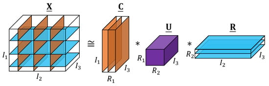
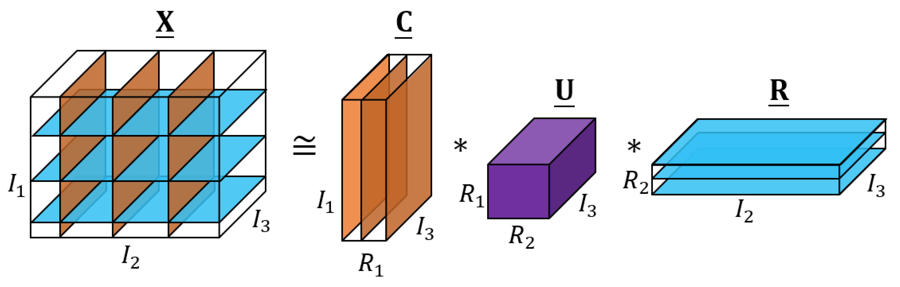
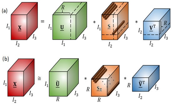
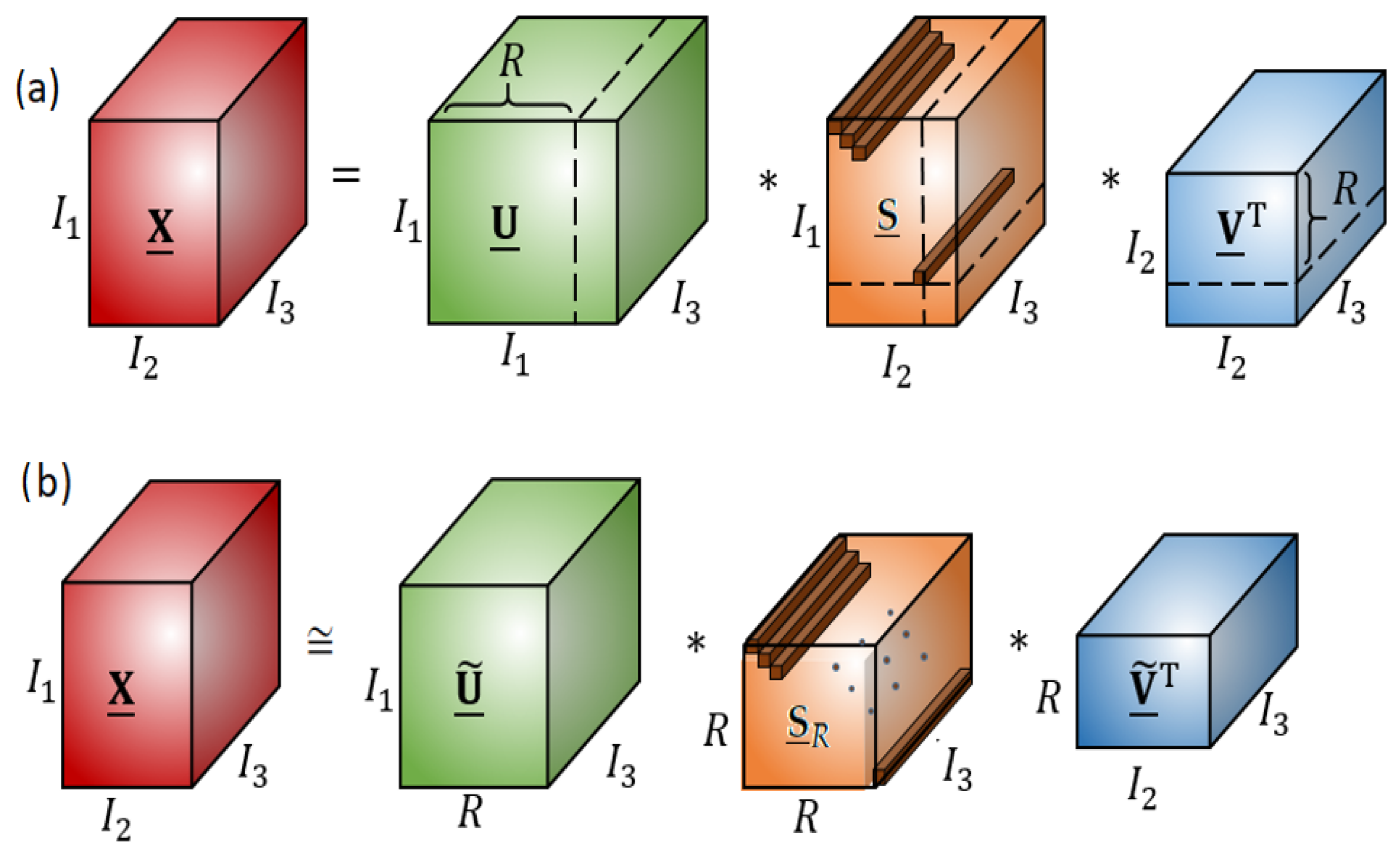
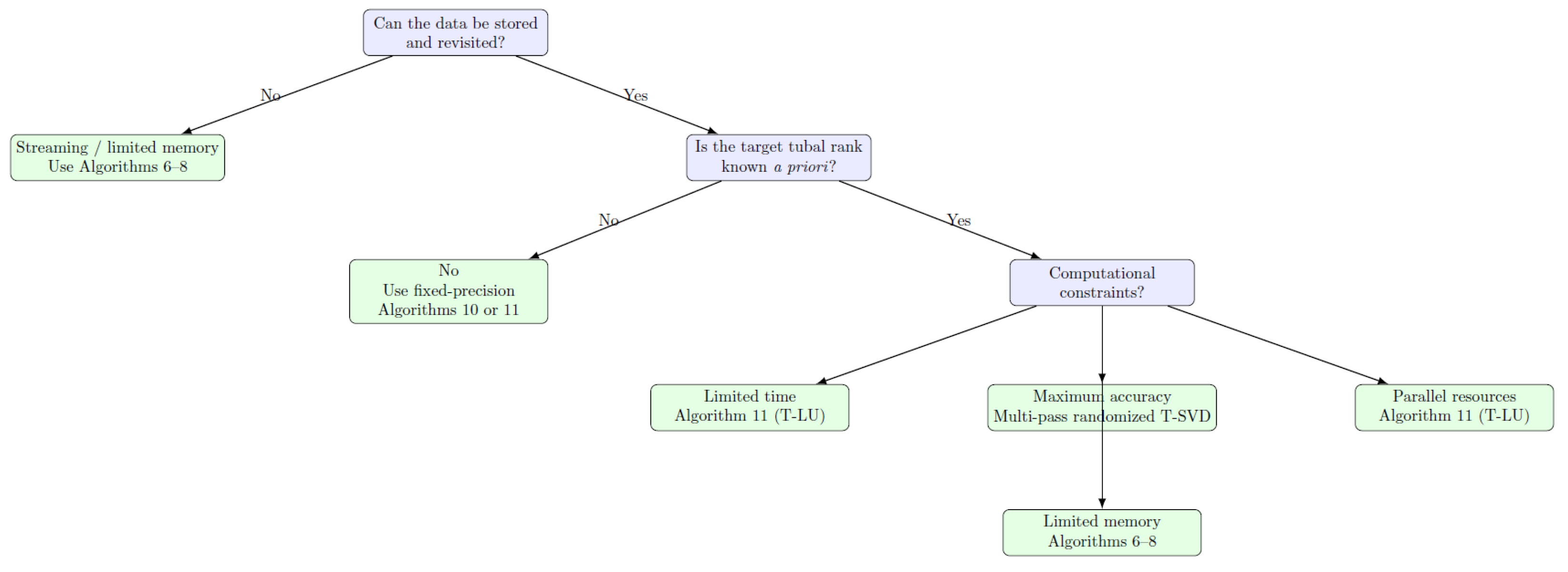
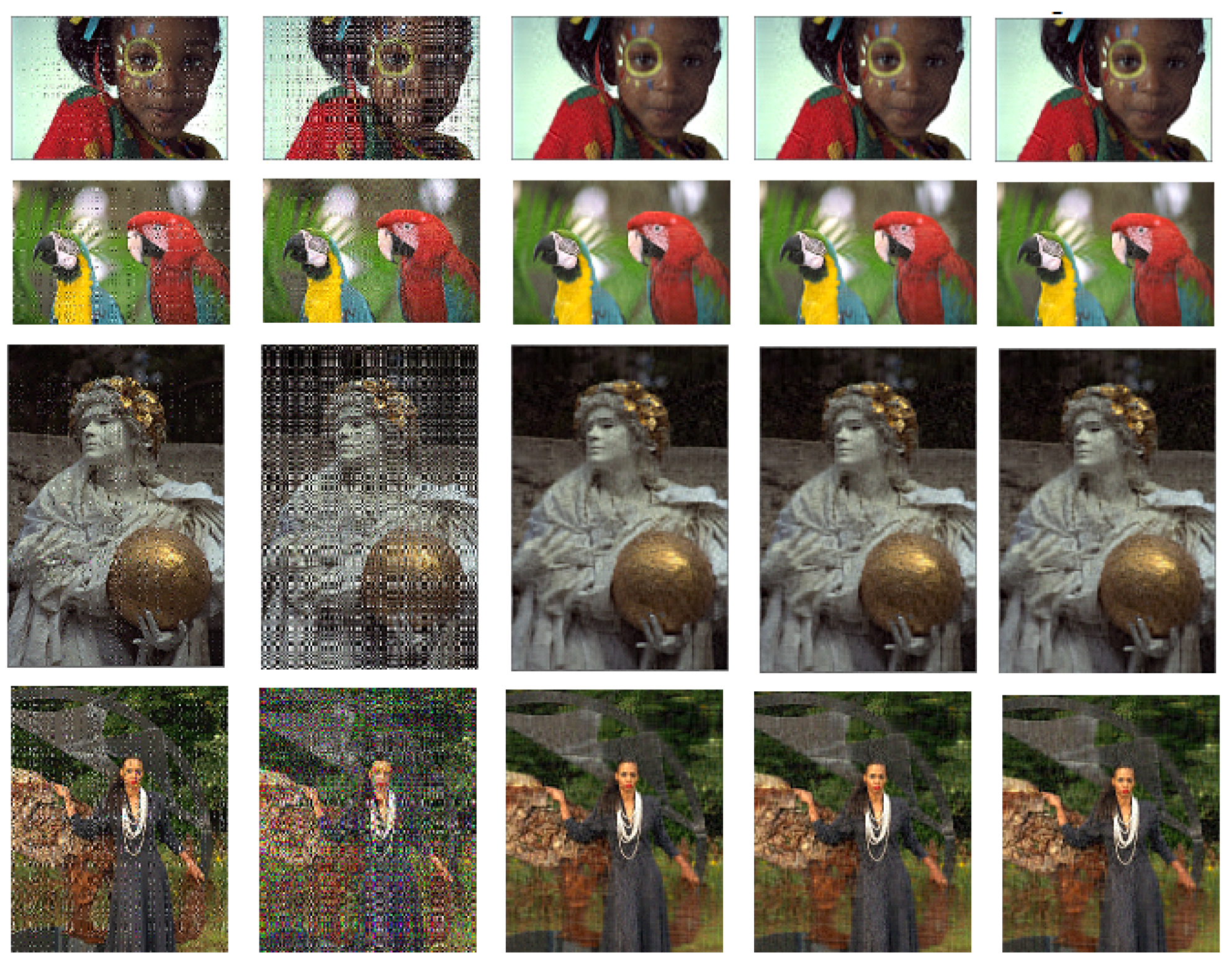
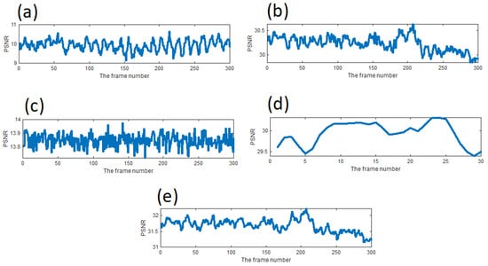
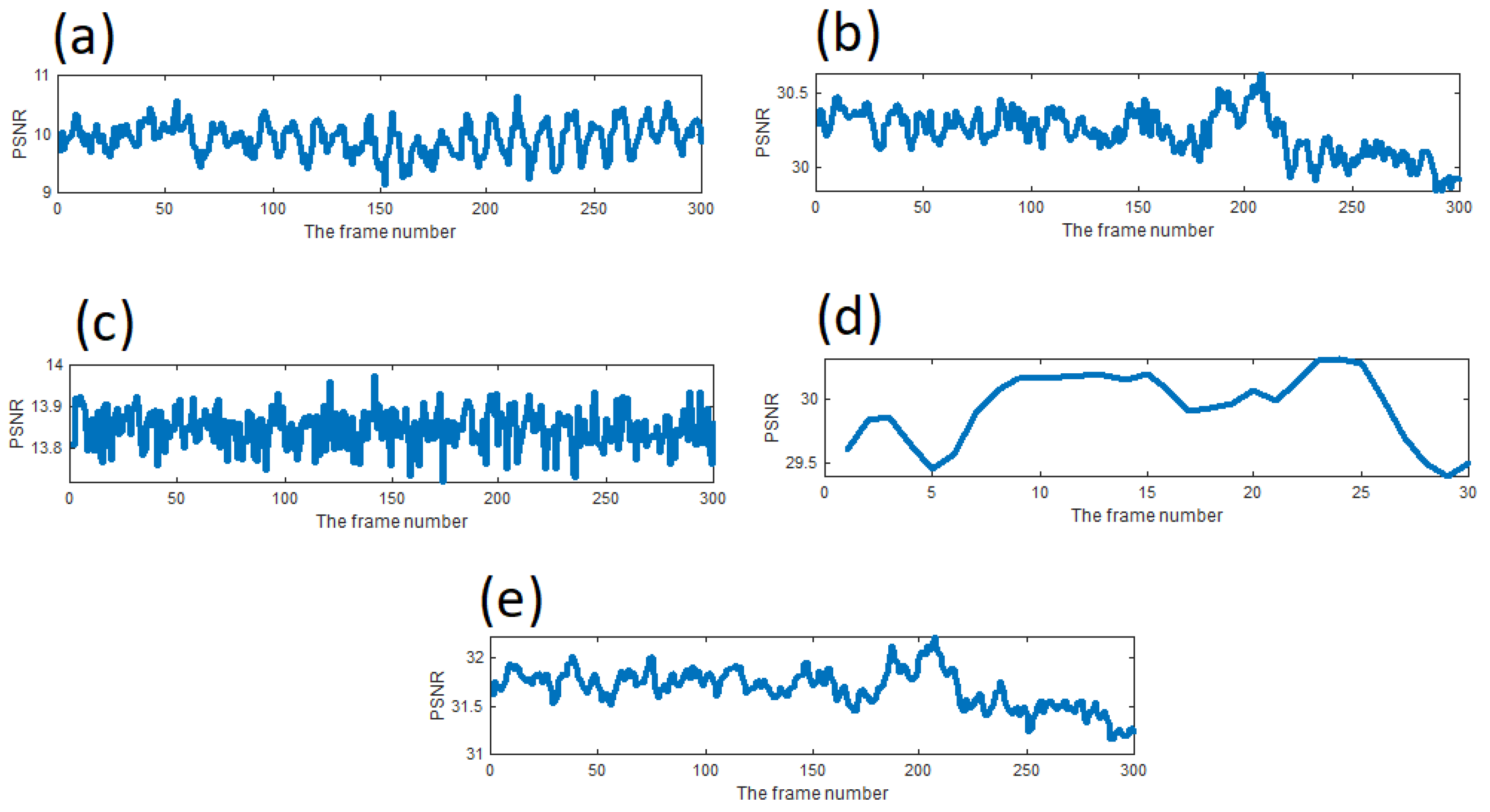
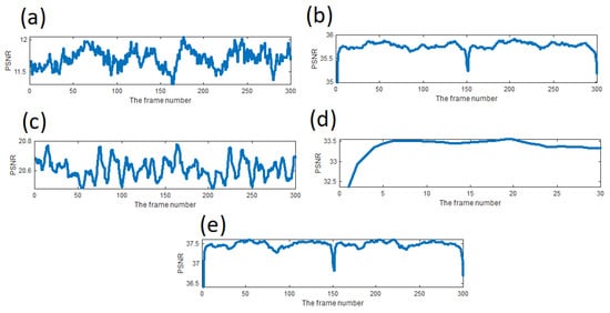
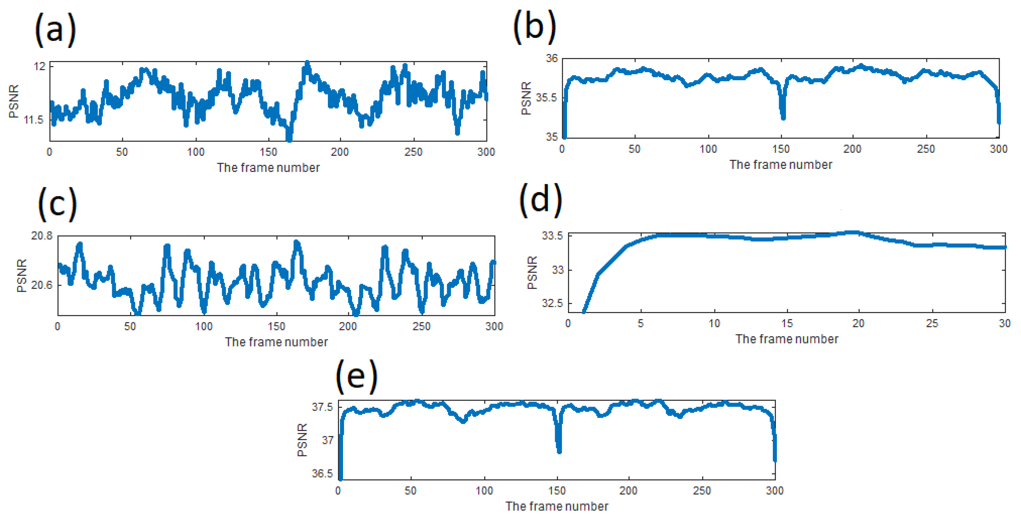
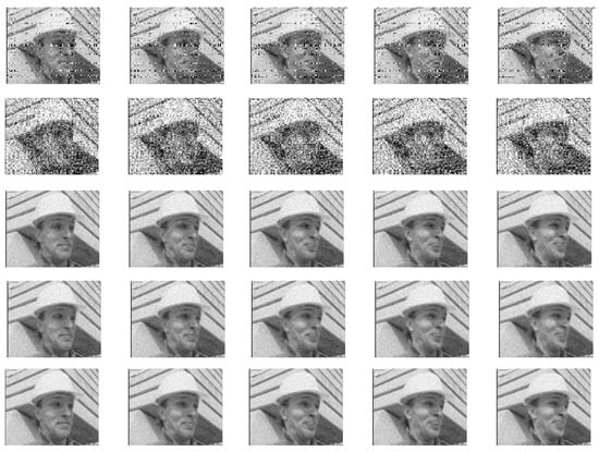
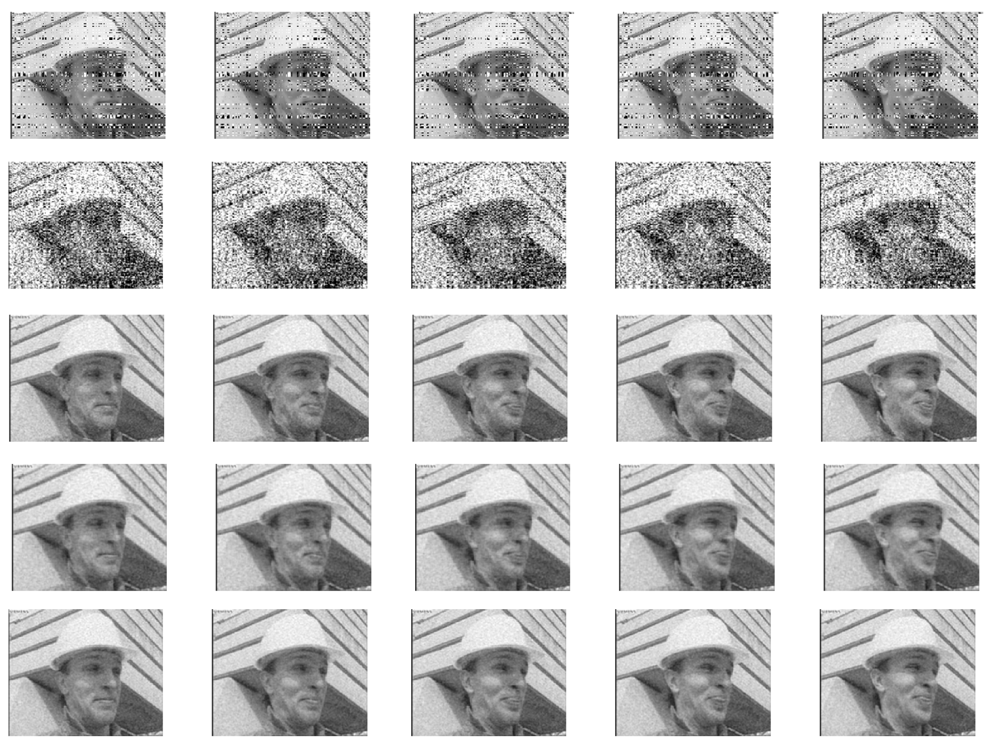
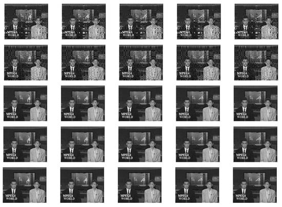
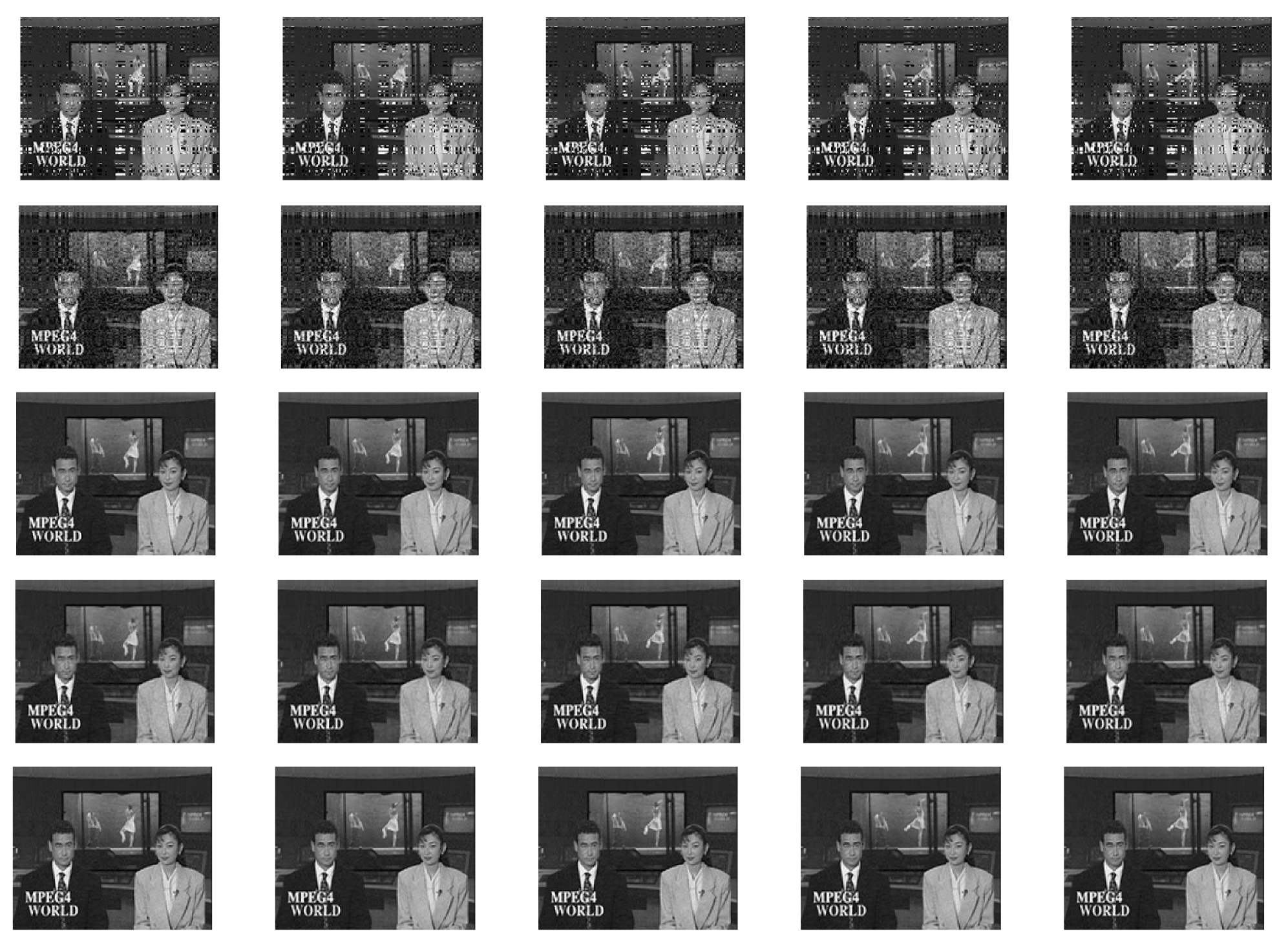
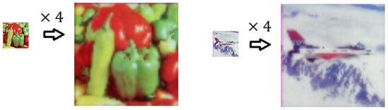
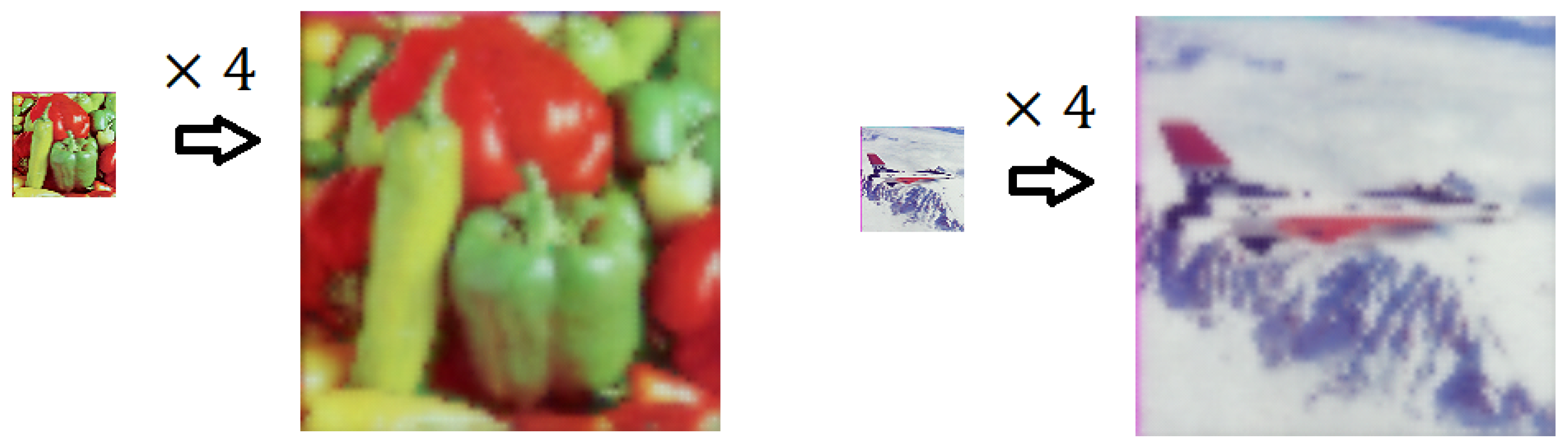
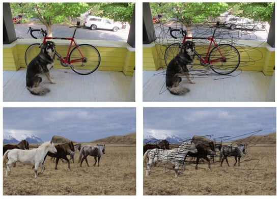
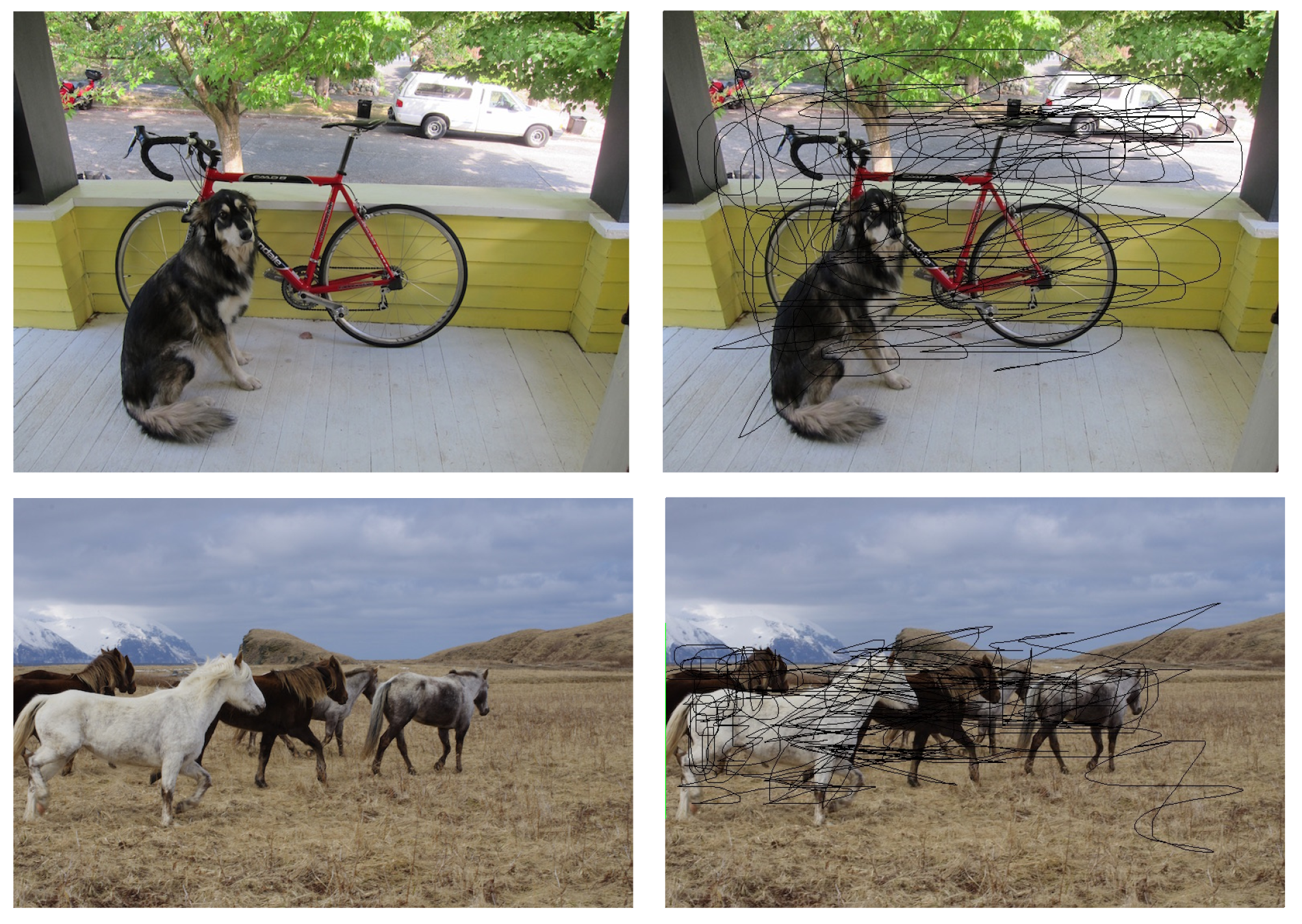
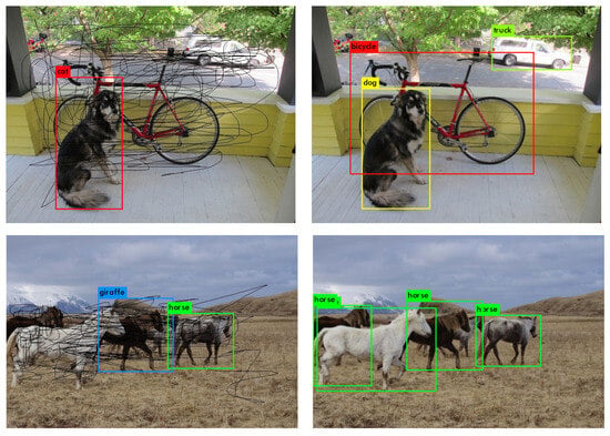
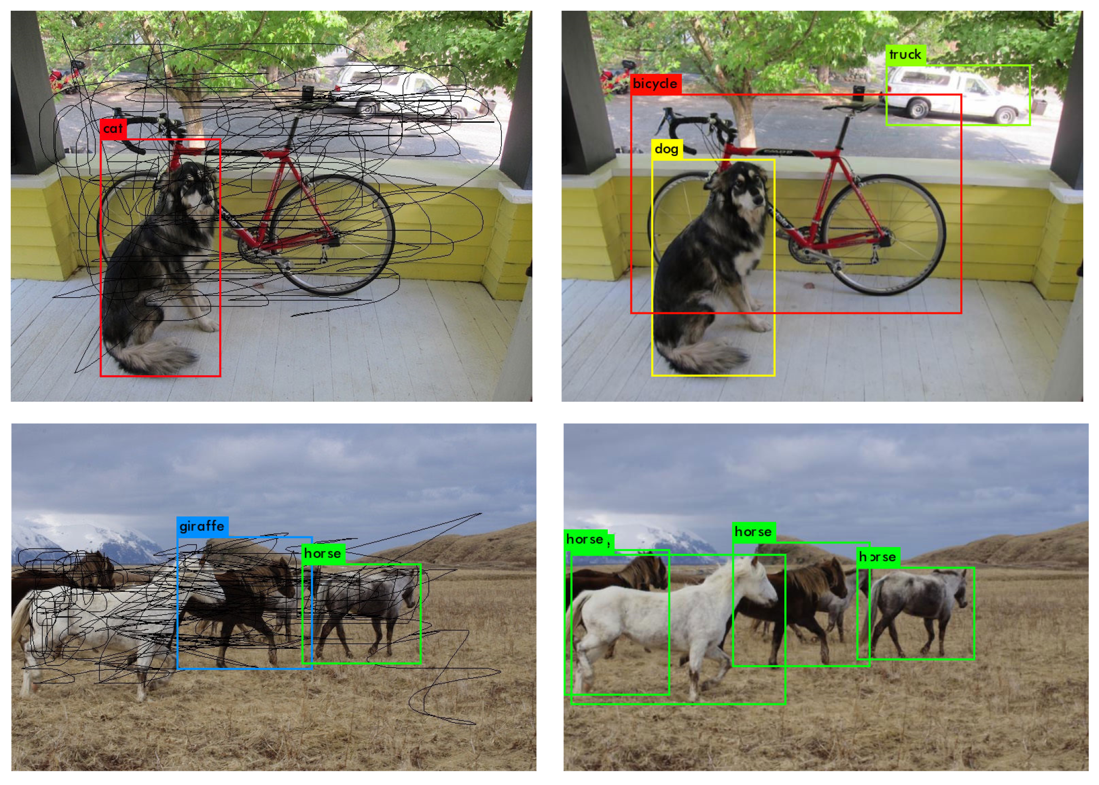

Disclaimer/Publisher’s Note: The statements, opinions and data contained in all publications are solely those of the individual author(s) and contributor(s) and not of MDPI and/or the editor(s). MDPI and/or the editor(s) disclaim responsibility for any injury to people or property resulting from any ideas, methods, instructions or products referred to in the content. |
© 2026 by the authors. Licensee MDPI, Basel, Switzerland. This article is an open access article distributed under the terms and conditions of the Creative Commons Attribution (CC BY) license.