Compressive Strength Prediction of Self-Compacting Concrete with Recycled Coarse Aggregate Using Machine Learning: Robust Multi-Split Evaluation and Data-Leakage Analysis of a Stacking Ensemble

Abstract

Reliable prediction of the compressive strength of self-compacting concrete with recycled coarse aggregate (SCRCAC) from mixture composition supports more rational mix design and fewer experimental tests. Using the benchmark dataset of the reference study (603 mixtures, eight input variables), this work re-examines machine-learning prediction of this property with an emphasis on honest evaluation rather than on a new model. A stacking ensemble of three gradient-boosting models (XGBoost, LightGBM, CatBoost) and an extremely randomized trees model, combined through a ridge meta-learner, is used as a representative model and compared with the four machine-learning models of the reference study (Random Forest, Extra Trees, XGBoost, LightGBM), the recent single-booster model of Abood et al., and the reference artificial neural network. Reported as the mean over 25 repeated 70/30 splits, the ensemble reaches R² = 0.793 ± 0.038 and RMSE = 6.21 ± 0.48 MPa, above all four reference models (R² = 0.7249–0.7635) and significantly, though only marginally, above a tuned single XGBoost. The central contribution is the evaluation itself. Because the dataset contains repeated identical compositions, a leakage-free protocol lowers the R² of every model to between 0.60 and 0.71, showing that the values of about 0.81–0.87 usually reported are inflated by duplicate-composition leakage, and leave-one-source-out evaluation lowers it further to about 0.14. Mutual-information and partial-dependence analyses identify cement as the dominant predictor, with water acting mainly through a nonlinear dependence. Robust, leakage-aware evaluation, rather than model architecture, emerges as the key to credible strength prediction on this benchmark.

1. Introduction

The construction industry is one of the largest single sources of carbon-dioxide emissions, with concrete production estimated to account for about 8% of global CO₂ emissions [1]. At the same time, excessive extraction of natural coarse and fine aggregate leads to resource depletion and rising costs, while demolition and reconstruction generate large amounts of construction waste that occupies land and burdens the environment [2]. The use of recycled coarse aggregate, obtained by crushing old concrete, mitigates both problems simultaneously and represents one of the pillars of the circular economy in construction [3,4]. Alternative mixture compositions are also being investigated, such as the use of volcanic aggregates, which demonstrate how strongly the choice of constituents shapes both the mechanical and the ecological properties of concrete [5].

Recycled aggregate, however, differs substantially in its properties from natural aggregate. A layer of old cement mortar remains on the grains, increasing porosity and water absorption (typically 3–9%), reducing density, and creating a weaker interfacial transition zone (ITZ) between the old and the new binder [1,6]. The consequences are a greater tendency toward segregation and bleeding in the fresh mixture and a drop in compressive strength, which at higher recycled-aggregate contents can reach 15% or more [1]. In self-compacting concrete, which flows and consolidates under its own weight without vibration, these effects are further pronounced because of its high sensitivity to fines content, the water-to-binder ratio, and the superplasticizer dosage [7,8].

Predicting the strength of such a heterogeneous material from its mixture composition using classical, empirical expressions, above all Abrams’ law of the water-to-cement ratio, yields large deviations, because these expressions cannot capture the nonlinear, synergistic effects of the microstructure of recycled aggregate and a high fines content [2,9]. The alternative is to rely on numerous trial mixtures and laboratory tests, which is costly and time-consuming [1]. Hence the growing need for predictive models that reliably estimate compressive strength from composition and reduce the volume of experimental work. Beyond the single test, this matters at the scale of a whole mix-design campaign. Qualifying a self-compacting recycled-aggregate mixture usually calls for a series of trial batches, often ten or more across the targeted strength classes, each consuming cement, aggregate, water, and admixtures and producing waste. A model that screens compositions reliably before casting can remove a large share of these trials, together with the associated material use and embodied carbon, which is directly in line with the United Nations Sustainable Development Goals on industry, innovation, and infrastructure (SDG 9), sustainable cities and communities (SDG 11), and responsible consumption and production (SDG 12).

Over the past decade, machine-learning and artificial-intelligence methods have proven to be a powerful tool for this task, as they learn complex nonlinear dependencies directly from data, without assuming a mathematical form of the relationship [2,4]. Artificial neural networks and, increasingly, tree-based ensembles have been applied to predicting the strength of recycled-aggregate concrete with high accuracy. A detailed review of these works is given in Section 2. The application of artificial intelligence in concrete technologies today ranges from predicting mechanical properties to mapping entire research fields [10]. Individual models, however, have their weaknesses and a sensitivity to the choice of the data split.

In the reference study by Jagadesh et al. [1], an artificial neural network and four machine-learning models (Random Forest, Extra Trees, XGBoost, LightGBM) were compared for the problem of predicting compressive strength from eight known input variables. The present work revisits this benchmark, but with a different emphasis. Its contribution is primarily methodological and empirical rather than a claim of a new algorithm, and it has three parts. First, a stacking ensemble of heterogeneous learners is used as a strong, representative model, and its performance is assessed against the models from the reference study. Second, and more importantly, performance is reported not for a single split but as the mean over 25 repeated 70/30 partitions, so that the stated accuracy reflects the typical behavior of the model rather than one convenient division of the data. Third, the dataset is examined for repeated (identical) compositions, and the effect of the resulting data leakage on the reported accuracy is quantified. This concern applies to every model trained on this benchmark and, as far as we are aware, has not been addressed in the studies that use it.

2. Literature Review

The application of artificial-intelligence methods to predicting the compressive strength of recycled-aggregate concrete has been developing for more than a decade, with a clear gradual evolution from simple neural networks toward more complex and more reliable machine-learning models. Early works confirmed the superiority of artificial neural networks (ANNs) over classical linear regression in modeling the nonlinear dependence of strength on mixture composition [2,3], establishing ANNs as a reliable substitute for time-consuming laboratory testing. In parallel, soft-computing models have also been successfully applied to related problems in civil engineering, such as the bond strength of FRP bars in concrete [11].

The next research phase focused on the network architecture and the choice of training algorithm. de-Prado-Gil et al. [7] systematically compared three algorithms, namely Levenberg–Marquardt, Bayesian Regularization (BR), and scaled conjugate gradient, and showed that BR is the most suitable for heterogeneous recycled material because it statistically suppresses overfitting. Similar methodological optimizations of ANNs appear for specific eco-concretes. Boudali et al. [6] modeled the influence of fine recycled concrete powder (FRCP) as a micro-filler, demonstrating that a content of up to 40% increases strength at later curing ages, while Nikmehr et al. [12] achieved exceptional accuracy on a strictly controlled database for one-part geopolymer SCC with coated recycled aggregate. de-Prado-Gil et al. [13] introduced a partitioning of the database into groups according to target compressive strength and derived explicit equations usable by engineers, while the reference study on which this work is based [1] compared an ANN with four machine-learning models (Random Forest, Extra Trees, XGBoost, LightGBM) on a dataset of more than 600 mixtures.

A key trend in recent research is the shift from individual neural networks toward tree-based ensemble methods and their interpretation. Several independent studies have shown that ensembles often outperform ANNs in reliability and physical consistency. Yang, Sun, and Xu [14] found that Random Forest yields more logically consistent results than an ANN; Yang, Chen, and Xu [15] confirmed the superiority of Random Forest using SHAP analysis and the a20-index as a measure of engineering reliability; and Almutairi [8] showed that gradient boosting (XGBoost) models the complex behavior of recycled concrete more efficiently than a classical ANN. On high-performance concrete, Alyaseen et al. [9] reported weaker generalization of ANNs compared with alternative models. The common conclusion of these works is that tree-based models offer a better balance of accuracy, stability, and interpretability. This conclusion is not limited to compressive strength. These models have already found use in solving other problems in civil engineering as well. Thus, explainable models with metaheuristic optimization [16] and ensemble models have found use for the fresh properties of concrete [17] and successfully cover other properties of self-compacting concrete as well. Hybrid generative–ensemble approaches are being applied to the properties of recycled-aggregate concrete [18], and systematic analyses confirm the robustness of gradient boosting even under demanding data conditions outside civil engineering [19]. Recent work continues in this direction with interpretable, optimization-tuned deep-learning models for the strength of alternative and sustainable concretes, such as an enhanced-bat-algorithm-optimized, chemistry-informed network for fly-ash/slag geopolymer concrete [20] and an attention-based CNN-LSTM model for rubberized concrete [21]. Both report high accuracy while placing explicit weight on model interpretability, which is the same concern that motivates the importance analysis reported later in this paper.

The work most similar to this one is the recently published paper by Abood et al. [22], who applied a single gradient-boosting model optimized by Bayesian optimization (BO-GBRT) on the same dataset [1], together with SHAP analysis and a web application, reporting a five-fold cross-validation R² = 0.806 and, on a single 90/10 split, a test R² = 0.868. Their approach, however, relies on a single booster and on an estimate from a single split, without verifying robustness across multiple splits and without considering the repetition of identical compositions in the dataset. The proposed stacking ensemble differs from the solution of those authors [22] both in architecture (a heterogeneous ensemble with a meta-learner instead of a single boosting tree) and in evaluation methodology, with a detailed comparison presented in Section 5.

The stacking architecture with a ridge meta-learner has also recently been confirmed in combination with deep learning. Dong and Zhang [23] combine, on a related dataset of self-compacting concrete with recycled aggregate (289 mixtures, 18 variables), an FT-Transformer and a masked multilayer perceptron precisely through a two-level stacking with a ridge meta-model, with conformal uncertainty intervals and an emphasis on robustness to missing data. Their results (R² = 0.940 on their own dataset) are not directly comparable with the present work because of the different dataset and richer mixture description, but they confirm the soundness of the stacking approach in this field. The research presented in this work differs in that it combines heterogeneous gradient-boosting models on the reference benchmark dataset [1] and evaluates performance robustly, over 25 repeated splits.

Two gaps emerge from this review, and together they motivate the present study. The first concerns evaluation. Almost all studies on this problem, including the most accurate recent ones, report performance on a single train/test split. Such a split can be unrepresentative, yet its stability is rarely checked across many repeated partitions. The second concerns data quality. The benchmark dataset used here and in related work contains repeated (identical) compositions, some with conflicting recorded strengths, and if these are not handled before splitting the same composition can fall into both the training and the test set, which biases the reported accuracy upward. Neither issue is tied to a particular model. Both affect every method evaluated on this dataset. The present paper addresses them directly, using a heterogeneous stacking ensemble with a ridge meta-learner as the working model, reporting performance over 25 repeated 70/30 splits, and quantifying how much of the accuracy on this benchmark is due to repeated-composition leakage. Table 1 positions the present study against the most closely related work [1,22,23].

Table 1. Comparison of the present study with the most closely related work on this dataset.

Study	Model	Dataset (n; Inputs)	Evaluation Protocol	Repeated-Composition Leakage	Reported R2
Jagadesh et al. [1]	ANN and four ML models (RF, ET, XGBoost, LightGBM)	603; 8	Single 70/30 split	Not addressed	ANN 0.86; ML 0.72–0.76
Abood et al. [22]	Single gradient boosting (Bayesian-optimized)	603; 8	5-fold CV; single 90/10 split	Not addressed	CV 0.806; 90/10 0.868
Dong and Zhang [23]	FT-Transformer and MLP via ridge stacking	289; 18	Own split with conformal intervals	Not addressed	0.940 (own dataset)
This work	Heterogeneous stacking (XGBoost, LightGBM, CatBoost, Extra Trees) with ridge	603; 8	25 repeated 70/30 splits; leakage-free and leave-one-source-out	Quantified; leakage-free R2 reported	0.793 (leaky); 0.60–0.71 (leakage-free); 0.14 (cross-source)

3. Dataset

For this research, the publicly available dataset presented in the reference study [1] was used. The authors compiled it through a systematic literature review, collecting SCRCAC mixtures from 57 published sources over 14 years. Although the reference study reports 602 mixtures, the Supporting Information file of that study contains 603 data rows. All 603 are used here, and this one-row discrepancy is noted for full transparency. Each mixture is described by eight input variables and the measured 28-day compressive strength (f_ck), given in Table 2. The heterogeneity of the sources (different laboratories, materials, and recipes) introduces realistic noise into the data but also makes the model more robust to diverse conditions.

Table 2. Description of variables.

Symbol	Description	Unit
Cement	Cement content	kg/m3
Water	Water content	kg/m3
FA	Natural fine aggregate	kg/m3
RFA	Recycled fine aggregate	kg/m3
CA	Natural coarse aggregate	kg/m3
RCA	Recycled coarse aggregate	kg/m3
MA	Mineral admixture	kg/m3
CHA	Chemical admixture (superplasticizer)	kg/m3
fck	28-day compressive strength (output)	MPa

Descriptive statistics of all input variables and of the output variable are given in Table 3. Cement content ranges from 78 to 635 kg/m³ and water from 105 to 277 kg/m³. Zeros for the aggregate fractions (FA, RFA, CA, RCA) correspond to mixtures that do not contain the respective component (for example, those with exclusively natural or exclusively recycled aggregate), so the large standard deviations of these variables reflect different degrees of replacement. One extreme value of the chemical admixture is also notable (CHA = 320 kg/m³, against a mean of 6.05 kg/m³), about 21 standard deviations above the mean and the only value beyond three standard deviations on any input, most likely originating from a unit or data-entry error. It was kept in the main analysis for exact comparability with the reference study, and its influence was checked separately, as reported below.

Table 3. Descriptive statistics of the input and output variables.

Variable	Mean	Std	Min	Max	Unit
Cement	362.22	107.94	78.0	635.0	kg/m3
Water	183.72	26.98	105.0	277.0	kg/m3
FA	684.09	295.08	0.0	1200.0	kg/m3
RFA	157.91	268.91	0.0	1200.0	kg/m3
CA	426.75	332.45	0.0	1170.0	kg/m3
RCA	334.46	323.59	0.0	1115.0	kg/m3
MA	153.74	109.58	0.0	449.0	kg/m3
CHA	6.05	14.62	0.0	320.0	kg/m3
fck	43.62	13.77	7.17	81.9	MPa

An additional data-quality analysis revealed that the 603 rows correspond to 504 unique compositions. A total of 84 groups of mixtures share an identical composition, and in 21 of these groups the same composition is associated with different measured strengths. Such contradictory duplicates represent irreducible noise that limits the maximum attainable coefficient of determination. Moreover, if they are not removed before splitting, identical compositions can “leak” between the training and test sets (data leakage) and artificially inflate the reported accuracy. For direct comparability with the reference study [1], the original dataset of 603 rows is retained here, with full awareness of this limitation and its discussion in the results.

The influence of this extreme value on the results was examined directly, since tree-based models can in principle be sensitive to outliers. Three versions of the data were compared under the same repeated 70/30 protocol: the untreated data, removal of the single point beyond three standard deviations, and winsorization of the chemical-admixture column at its 99th percentile. The stacking ensemble gave a mean R² of 0.793 (untreated), 0.788 (removal), and 0.793 (winsorization). A tuned XGBoost behaved almost identically (0.786, 0.782, and 0.786). All of these differences are far smaller than the split-to-split scatter (standard deviation about 0.038), so the extreme value does not materially affect the reported accuracy. Because removing or capping it brings no benefit, and to keep the comparison with the reference study exact, the untreated 603-row data are used throughout the remainder of the paper. The three treatments are compared in Table 4.

Table 4. Sensitivity of the results to the chemical-admixture outlier (mean R² ± standard deviation over 25 repeated 70/30 splits).

Treatment	n	Proposed Stacking	Tuned XGBoost
Untreated (603 rows)	603	0.793 ± 0.038	0.786 ± 0.038
Outlier removed (beyond 3σ)	602	0.788 ± 0.028	0.782 ± 0.033
Winsorized at 99th percentile	603	0.793 ± 0.038	0.786 ± 0.038

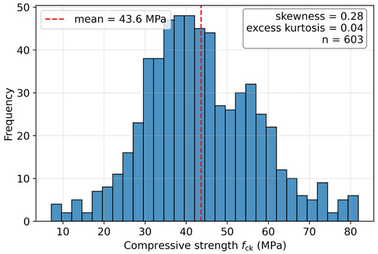
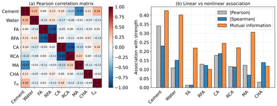
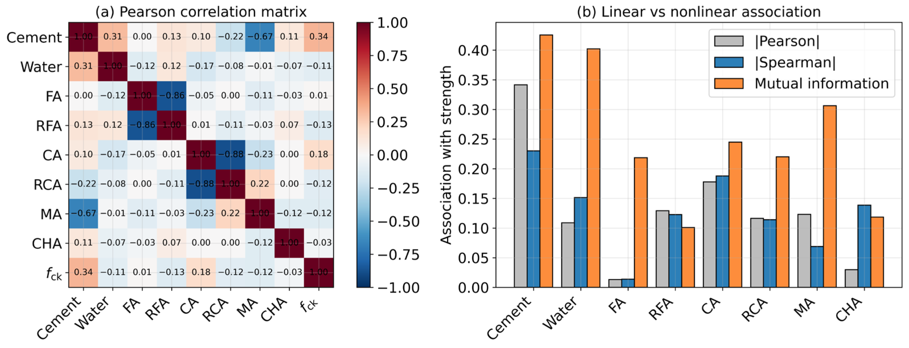
Compressive strength ranges from 7.2 to 81.9 MPa, with a mean of 43.6 MPa. The distribution is only mildly right-skewed (skewness 0.28, excess kurtosis 0.04) and close to symmetric, as Figure 1 shows. Linear correlations with strength are weak for every input (Figure 2a), the strongest being with cement at r = 0.34. A weak linear correlation, however, does not by itself establish a nonlinear relationship, so Spearman rank correlations and mutual-information scores were computed as well. These give a fuller picture (Figure 2b). Water, for example, is almost linearly uncorrelated with strength (Pearson r = −0.11) yet has one of the highest mutual-information scores (0.40), a clear sign of a nonlinear dependence that a linear coefficient cannot capture. This combination of weak linear but appreciable nonlinear association across the inputs is exactly the regime in which tree-based ensembles tend to perform well.

Figure 1. Distribution of the target variable (compressive strength).

Figure 2. (a) Pearson correlation matrix of the input and output variables. (b) Linear versus nonlinear association with the compressive strength, showing the absolute Pearson and Spearman correlations and the mutual-information score of each input.

4. Methodology

4.1. Underlying Techniques and Theoretical Background

The proposed model belongs to the field of artificial intelligence (AI), more precisely to its subfield of machine learning (ML). Machine learning encompasses algorithms that learn the dependence between inputs and outputs directly from data, without explicitly programmed rules. When a known output is associated with each input example, this is supervised learning. If the output is a continuous quantity, such as compressive strength, the problem is called regression. For structured (tabular) data, a particularly successful class is the ensemble methods based on decision trees, which combine a large number of simple models into a single accurate and stable model. Developed during the 1990s and 2000s (bagging, random forests, gradient boosting), they are today regarded as the standard for tabular data, often outperforming neural networks on datasets of moderate size. The building blocks of the proposed ensemble are described in turn below.

Decision tree (CART). The basic building block of all the models used is the decision tree, formalized in the work of Breiman, Friedman, Olshen, and Stone [24]. A regression tree recursively partitions the input space into disjoint regions through binary splits of the form “variable ≤ threshold,” predicting a constant in each leaf (terminal region). For a given split of a set into a left (L) and a right (R) subset, the optimal variable and threshold are chosen by minimizing the sum of squared deviations:

$$\mathrm{S}\mathrm{S}\mathrm{E}(s)={\sum }_{i\in L}(y_i-{\overline{y}}_L{)}^2+{\sum }_{i\in R}(y_i-{\overline{y}}_R{)}^2$$

(1)

where ${\overline{\mathrm{y}}}_L$ and ${\overline{\mathrm{y}}}_R$ are the mean target values in the left and right subsets. The prediction in leaf R_m equals the average of the target values of the samples falling into it:

$${\widehat{y}}_{R_m}={\displaystyle \frac{1}{\left|R_m\right|}}{\sum }_{i\in R_m}{y}_i$$

(2)

Equation (2). The key tunable parameters of a tree are the maximum depth, the minimum number of samples per node/leaf, and the splitting criterion. A single tree has high variance (it is sensitive to the data), which is the main motivation for the ensemble methods that reduce this variance.

Bagging (bootstrap aggregation) [25] trains multiple trees on bootstrap samples of the training set and averages their predictions, thereby reducing variance:

$$\widehat{f}(x)={\displaystyle \frac{1}{B}}{\sum }_{b=1}^B{T}_b(x)$$

(3)

Equation (3), where B is the number of trees. Random forests [26] additionally select a random subset of variables at each split. Extra Trees (extremely randomized trees) [27] go a step further: the threshold of each split is chosen at random, and the entire training set is used (without bootstrapping). This further reduces variance at a slight increase in bias, and training is very fast. The tunable parameters are the number of trees, the number of random variables per split, and the depth.

Unlike bagging, which builds trees independently, gradient boosting [28] builds an additive model sequentially, with each successive tree correcting the errors of the sum of the previous ones:

$$F_M(x)=F_0(x)+{\sum }_{m=1}^M\nu {\gamma }_m{h}_m(x)$$

(4)

where F₀ is the initial constant, h_m the m-th tree, γ_m its coefficient, and ν the learning rate. The model is initialized with the constant that minimizes the loss function L:

$$F_0(x)=\mathrm{a}\mathrm{r}\mathrm{g}\hspace{0.17em}{min}_{\gamma }{\sum }_{i=1}^{n}L(y_i,\gamma )$$

(5)

Equation (5). At each iteration m, the pseudo-residuals are computed as the negative gradient of the loss function with respect to the current prediction:

$$r_{im}=-{\left[{\displaystyle \frac{\partial L(y_i,F(x_i))}{\partial F(x_i)}}\right]}_{F=F_{m-1}}$$

(6)

The new tree h_m is fit to these pseudo-residuals, and the model is updated with scaling by the learning rate ν, which acts as a regularizer (smaller ν → slower but more stable learning):

$$F_m(x)=F_{m-1}(x)+\nu {\gamma }_m{h}_m(x),0<\nu \le 1$$

(7)

The main parameters are the number of trees M, the learning rate ν, and the tree depth. Three modern implementations of gradient boosting, namely XGBoost, LightGBM, and CatBoost, differ in their regularization, tree-growth strategy, and efficiency, and thus introduce the desirable diversity into the ensemble.

XGBoost [29] is an efficient, regularized implementation that minimizes an objective composed of a loss function and a complexity term:

$$L={\sum }_{i=1}^{n}l(y_i,{\widehat{y}}_i)+{\sum }_k\mathit{\Omega }(f_k),\mathit{\Omega }(f)=\gamma T+{\displaystyle \frac{1}{2}}\lambda \Vert w{\Vert }^2$$

(8)

where Ω penalizes the number of leaves T and the norm of their weights w. The objective is approximated at each step by a second-order Taylor expansion:

$$L^{\left(t\right)}\simeq {\sum }_{i=1}^n\left[g_i{f}_t(x_i)+{\displaystyle \frac{1}{2}}{h}_i{f}_t^2(x_i)\right]+\mathit{\Omega }(f_t)$$

(9)

Here g_i and h_i are the first and second derivatives of the loss with respect to the current prediction:

$$g_i={\partial }_{{\widehat{y}}^{\left(t−1\right)}}l(y_i,{\widehat{y}}^{\left(t−1\right)}),h_i={\partial }_{{\widehat{y}}^{\left(t−1\right)}}^{2}l(y_i,{\widehat{y}}^{\left(t−1\right)})$$

(10)

For a fixed tree structure, the optimal leaf weight j and the gain at a node split are:

$$w_j^{*}=-{\displaystyle \frac{{\sum }_{i\in I_j}{g}_i}{{\sum }_{i\in I_j}{h}_i+\lambda }}$$

(11)

$$G={\displaystyle \frac{1}{2}}\left[{\displaystyle \frac{{\left({\sum }_{i\in I_L}{g}_i\right)}^2}{{\sum }_{i\in I_L}{h}_i+\lambda }}+{\displaystyle \frac{{\left({\sum }_{i\in I_R}{g}_i\right)}^2}{{\sum }_{i\in I_R}{h}_i+\lambda }}-{\displaystyle \frac{{\left({\sum }_{i\in I}{g}_i\right)}^2}{{\sum }_{i\in I}{h}_i+\lambda }}\right]-\gamma$$

(12)

A split is made only if the gain G is positive, so that γ acts as a pruning threshold. The main tunable parameters are: the number of trees (n_estimators), maximum depth (max_depth), learning rate (learning_rate), row subsampling (subsample) and column subsampling (colsample_bytree), the minimum leaf weight (min_child_weight), the L1 and L2 regularization (reg_alpha, reg_lambda), and the threshold γ (gamma).

LightGBM [30] accelerates boosting through two key techniques. Gradient-based One-Side Sampling (GOSS) keeps all instances with a large gradient (fraction a) and randomly samples a portion (fraction b) of the instances with a small gradient, compensating their weight by a factor of (1 − a)/b so that the gain estimate remains unbiased:

$${\tilde{V}}_j(d)={\displaystyle \frac{1}{n}}\left({\displaystyle \frac{{\left({\sum }_{x_i\in A_l}{g}_i+\frac{1-a}{b}{\sum }_{x_i\in B_l}{g}_i\right)}^2}{n_l^j(d)}}+{\displaystyle \frac{{\left({\sum }_{x_i\in A_r}{g}_i+\frac{1-a}{b}{\sum }_{x_i\in B_r}{g}_i\right)}^2}{n_r^j(d)}}\right)$$

(13)

Equation (13), where A is the set with a large and B the set with a small gradient. The second technique, Exclusive Feature Bundling (EFB), bundles sparse, mutually exclusive features into one, thereby reducing dimensionality. In addition, LightGBM uses histogram-based binning of values and leaf-wise growth instead of level-wise growth, choosing the leaf with the largest loss reduction. The main parameters are the number of leaves (num_leaves), depth, learning rate, subsampling, the minimum number of samples per leaf (min_child_samples), and regularization.

CatBoost [31] introduces ordered boosting, which, by using random permutations and models trained without the current instance, eliminates prediction-shift bias and implicit target leakage. It also uses symmetric (oblivious) trees, in which all trees at the same level share the same split condition, and this speeds up prediction and acts as a regularizer. The main parameters are the number of iterations, depth, learning rate, L2 regularization (l2_leaf_reg), random strength, and the sampling temperature.

Stacking (stacked generalization) [32] combines heterogeneous base models by making their predictions the input to a meta-model that learns the optimal combination. To avoid leakage, the predictions of the base models used to train the meta-model are generated by cross-validation (out-of-fold):

$$z_i=\left({\widehat{h}}_1^{\left(-k\right)}(x_i),\dots ,{\widehat{h}}_K^{\left(-k\right)}(x_i)\right)$$

(14)

In Equation (14), (−k) denotes the model trained without the fold containing sample i. The meta-model used is ridge regression [33], which minimizes the squared error with an L2 penalty:

$$\widehat{w}=\mathrm{a}\mathrm{r}\mathrm{g}\hspace{0.17em}{min}_w{\sum }_{i=1}^n{\left(y_i−w^{\top }{z}_i\right)}^2+\lambda \Vert w{\Vert }^2$$

(15)

with the closed-form solution:

$$\widehat{w}={\left(Z^{\top }Z+\lambda I\right)}^{-1}{Z}^{\top }y$$

(16)

In Equations (15) and (16), Z is the matrix of meta-inputs. Ridge is suitable because the predictions of the base models are highly correlated (multicollinearity), so the L2 regularization stabilizes the weights, and the parameter λ is selected by cross-validation (RidgeCV). Stacking architectures have been successfully applied across the most diverse prediction domains [34].

4.2. Application to the Present Problem

The choice of the initial set of models was guided by the nature of the problem. The dataset is tabular, of moderate size (603 examples, eight variables), strongly nonlinear and noisy, with weak linear correlations. For such data, tree ensembles are the method of choice. Four complementary base models were selected: three implementations of gradient boosting (XGBoost, LightGBM, CatBoost), which learn similar dependencies but through different mechanisms of tree growth, regularization, and gradient handling, and Extra Trees, which belongs to the bagging family and introduces a substantially different (high-variance, weakly correlated) error component. It is precisely this diversity of errors that is the precondition for stacking to deliver improvement. The meta-learner exploits the parts where the models differ.

Theory-based expectations are that each booster individually achieves an R² of about 0.76–0.79 on this type of problem, while Extra Trees usually yields a somewhat lower but decorrelated result. Since stacking linearly combines complementary predictions, a stable performance in the upper part of that range is expected. The extent to which the best individual model is actually surpassed, and how much diversity among the base learners is truly present, is quantified in detail in Section 5.6, Section 5.7 and Section 5.8.

The ensemble has two levels. At level zero, all four models operate in parallel and independently on the same input, the matrix X of dimension n × 8 (eight numerical variables in kg/m³). The level-zero outputs are not passed to one another (there is no serial dependence among them). Their out-of-fold predictions form the meta-feature matrix Z of dimension n × 4, which is the input to the first level (the ridge meta-learner). Here a serial dependence exists, since the first-level output depends on the outputs of all level-zero models. The system output is a scalar (the predicted f_ck in MPa). Five-fold cross-validation within the stacking ensures that the meta-learner never sees the base-model predictions on the data on which those models were trained.

The three boosters were optimized once, with the Optuna library [35] (TPE search, five-fold cross-validation on the training portion of a single reference split), and the resulting configurations were then kept fixed and reused for all 25 repeated splits. The test data were never used during tuning. Extra Trees and the ridge meta-model were deliberately kept simple. The specific selected configurations are given in Table 5.

Table 5. Configuration of base models and the meta-learner.

Model	Key Tuned Hyperparameters
XGBoost	n_estimators = 695, max_depth = 6, learning_rate = 0.087, subsample = 0.96, colsample_bytree = 0.75, min_child_weight = 7, reg_alpha = 0.055, reg_lambda = 0.032, gamma = 0.005
LightGBM	n_estimators = 770, num_leaves = 45, max_depth = 10, learning_rate = 0.037, subsample = 0.54, colsample_bytree = 0.76, min_child_samples = 7, reg_alpha = 0.045, reg_lambda = 0.049
CatBoost	iterations = 872, depth = 5, learning_rate = 0.050, l2_leaf_reg = 0.027, random_strength = 0.034, bagging_temperature = 0.587
Extra Trees	default settings (random_state fixed), used as a decorrelated stabilizer
Ridge (meta)	RidgeCV: L2 penalty λ selected by internal cross-validation

For the boosters, precisely those parameters that control capacity and regularization are tuned (the number and depth of trees, the learning rate, subsampling, L1/L2 penalties), since they have the greatest influence on the bias–variance trade-off. Extra Trees was kept at its default values, because its role is not to be the most accurate individual model but to introduce a decorrelated component. Additional tuning did not bring consistent gains. The meta-learner is deliberately linear (ridge) with a single regularization parameter selected automatically, which avoids overfitting on only four meta-features. Five-fold (cv = 5) generation of the meta-features was chosen as the usual compromise between bias and computational cost.

4.3. Evaluation Protocol

For comparability, the 70% training/30% test split was retained, as in the reference study [1]. To avoid the bias of a single split, performance is reported as the mean ± standard deviation over 25 repeated random splits, with the same splits used for all models. Hyperparameter optimization was performed exclusively by inner five-fold cross-validation on the training set. The metrics used are the coefficient of determination, the root mean squared error, and the mean absolute error:

$$R^2=1-{\displaystyle \frac{{\sum }_{i=1}^n(y_i-{\widehat{y}}_i{)}^2}{{\sum }_{i=1}^n(y_i-\overline{y}{)}^2}}$$

(17)

$$\mathrm{R}\mathrm{M}\mathrm{S}\mathrm{E}=\sqrt{{\displaystyle \frac{1}{n}}{\sum }_{i=1}^n(y_i-{\widehat{y}}_i{)}^2}$$

(18)

$$\mathrm{M}\mathrm{A}\mathrm{E}={\displaystyle \frac{1}{n}}{\sum }_{i=1}^n\left|y_i−{\widehat{y}}_i\right|$$

(19)

Equations (17)–(19). The implementation is in Python 3.11.9 (Python Software Foundation, Wilmington, DE, USA) using the scikit-learn 1.8.0 [36], XGBoost 3.2.0 [29], LightGBM 4.6.0 (Microsoft Corporation, Redmond, WA, USA) [30], CatBoost 1.2.10 (Yandex, Moscow, Russia) [31], and Optuna 4.8.0 (Preferred Networks, Inc., Tokyo, Japan) [35] libraries.

Because the hyperparameters were fixed rather than re-optimized for every split, their influence was checked directly. On five of the splits the three boosters were re-tuned from scratch (Optuna, inner five-fold cross-validation on that split’s training set). The selected values varied considerably across splits, for example the XGBoost tree count was between 638 and 901 and its maximum depth was between 4 and 10 and the LightGBM leaf count was between 15 and 87, yet the resulting ensemble reached essentially the same test performance as the fixed configuration (R² = 0.800 ± 0.036 with per-split tuning versus 0.801 ± 0.035 with fixed parameters). Fixing the hyperparameters is therefore not a source of optimistic bias, and it keeps the repeated-split protocol computationally tractable.

Two further variants of the evaluation are used in the results to test its robustness. First, to confirm that the reported variability is not an artifact of unequal strength distributions, a stratified 70/30 split by strength quartile is compared with the plain random split. Second, and more importantly, a leakage-free protocol is applied. Because the dataset contains repeated (identical) compositions, a plain random split can place the same composition in both the training and the test set. Two remedies are therefore used, aggregating each repeated composition into a single averaged record (which reduces the 603 rows to 504 unique compositions) and group-aware splitting that keeps all rows of a given composition on the same side of the split. Standard k-fold cross-validation (five- and ten-fold) is also reported for comparison. All of these results are given in Section 5.

5. Results and Discussion

5.1. Robust Performance and Comparison

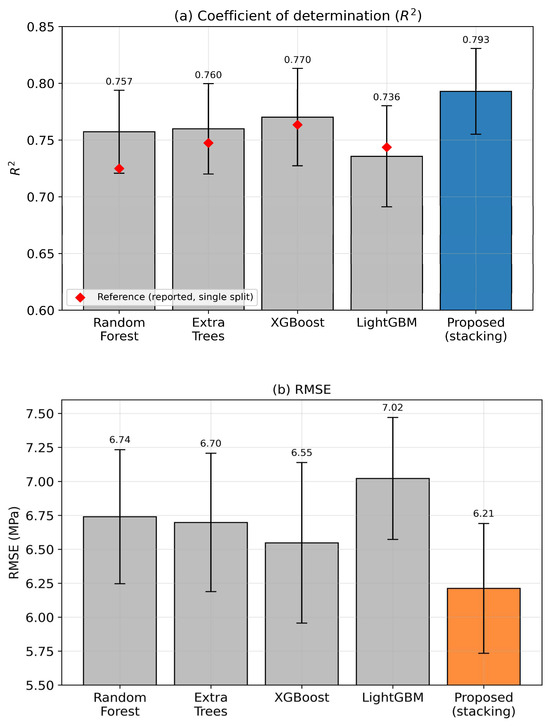
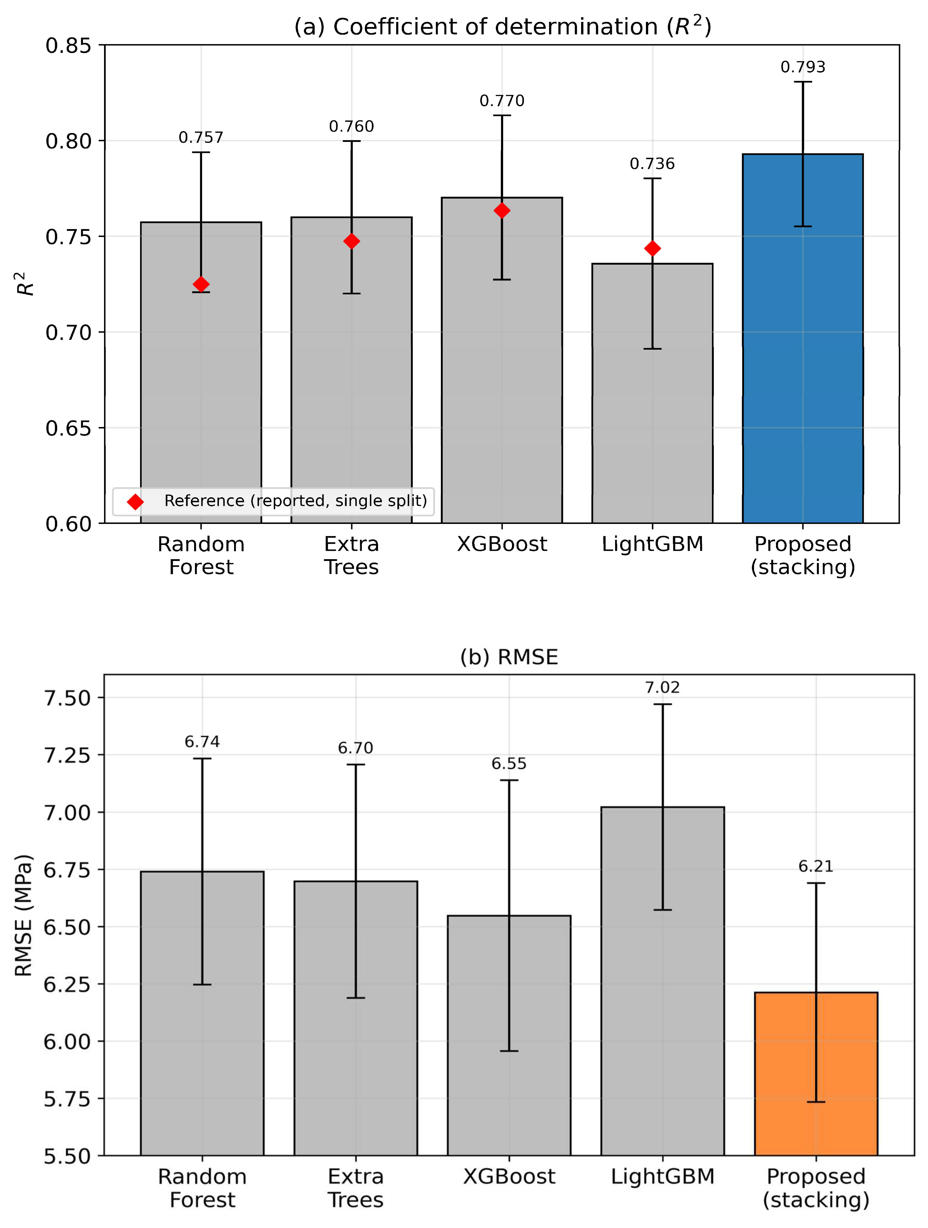
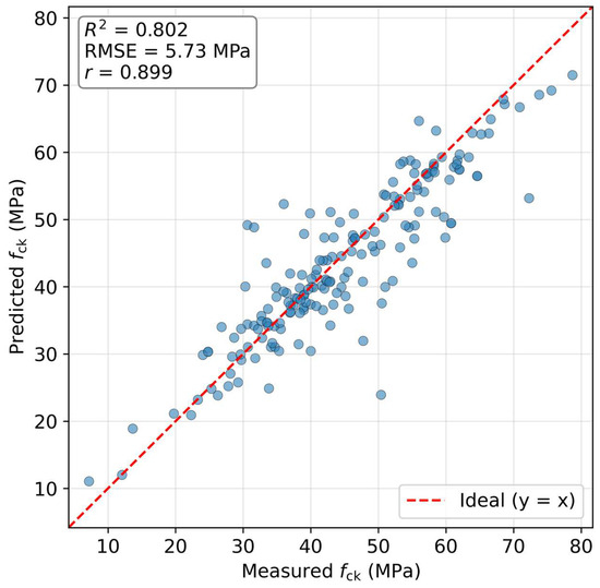
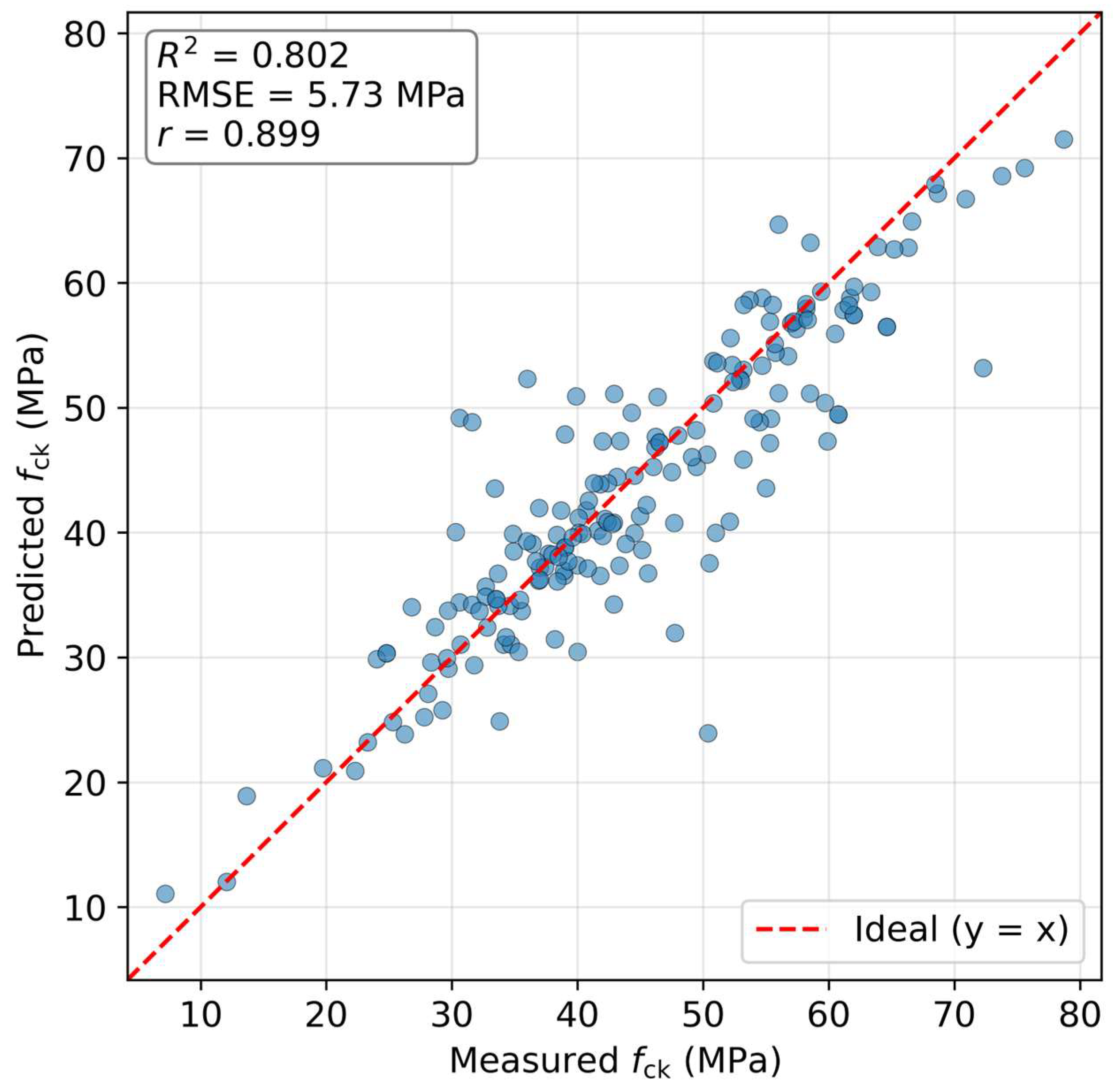
Under the repeated 70/30 protocol, the proposed stacking ensemble achieves R² = 0.793 ± 0.038, RMSE = 6.21 ± 0.48 MPa, MSE = 38.8 ± 6.0 MPa², and MAE = 4.06 ± 0.29 MPa. Table 6 presents the R², RMSE, and MSE values of the proposed ensemble and of the four machine-learning models from the reference study: R² = 0.793 and RMSE = 6.21 MPa for the proposed model, against the ranges R² = 0.7249–0.7635 and RMSE = 6.80–7.34 MPa for the reference models. The same comparison is shown in Figure 3. On a representative split, the model achieves R² = 0.802 with a correlation coefficient r = 0.899 (Section 5.5).

Table 6. Comparison with the reference study (proposed model: mean over 25 × 70/30). Bold indicates the proposed model.

Model	R2	RMSE (MPa)	MSE (MPa2)
Random Forest (reference)	0.7249	7.34	53.80
Extra Trees (reference)	0.7474	7.03	49.40
LightGBM (reference, default)	0.7437	7.08	50.13
XGBoost (reference, best)	0.7635	6.80	46.26
Proposed stacking ensemble	0.793	6.21	38.8

Figure 3. Comparison with the reference study over the matched 25-split protocol: (a) coefficient of determination (R²) and (b) RMSE. Bars show the mean and the error bars the standard deviation over 25 repeated 70/30 splits, while the red markers in panel (a) are the single-split values reported in the reference study [1].

5.2. Leakage-Aware Evaluation

The most consequential result of this study concerns data leakage rather than model ranking. As noted in Section 3, the 603 rows correspond to only 504 unique compositions, so a plain random split can place identical compositions in both the training and the test set. Two leakage-free protocols were therefore applied. When the repeated compositions are aggregated into 504 averaged records, the coefficient of determination of the proposed ensemble falls from 0.793 to 0.710 ± 0.048. A group-aware split, which keeps every composition entirely on one side of the split, lowers it further to 0.596 ± 0.053. The same drop affects every model on this dataset: under the aggregated protocol the four reference-type models fall to R² between 0.64 and 0.67, and the tuned single boosters to about 0.70. These results are collected in Table 7.

Table 7. Performance of each model under the leaky and the two leakage-free protocols (mean R² ± standard deviation over the repeated splits; dashes mark configurations not evaluated under the group-aware split).

Model	603-Row Random Split (Leaky)	504 Unique Compositions (Aggregated)	603 Rows, Group-Aware Split
Proposed stacking	0.793 ± 0.038	0.710 ± 0.048	0.596 ± 0.053
Tuned XGBoost	0.786 ± 0.038	0.699 ± 0.049	0.689 ± 0.051
Random Forest (default)	0.757 ± 0.037	0.667 ± 0.052	—
Extra Trees (default)	0.760 ± 0.040	0.644 ± 0.060	—
XGBoost (default)	0.770 ± 0.043	0.673 ± 0.055	—
LightGBM (default)	0.736 ± 0.045	0.640 ± 0.065	—

The magnitude of the effect can be measured directly. In a random 70/30 split of the 603 rows, about 22% of the test compositions also occur in the training set. In a 90/10 split the figure rises to 28%. These are exactly the protocols used by the earlier studies on this dataset [1,22], which report R² of roughly 0.81 to 0.87. Our results indicate that a substantial part of that reported accuracy reflects memorization of repeated compositions rather than genuine prediction, and that the leakage-free value, between 0.60 and 0.71 depending on the protocol, is the more honest estimate of predictive performance. Because the effect is a property of the benchmark rather than of any particular model, it applies equally to the ensemble proposed here.

Under the strictest, group-aware protocol the ensemble no longer holds an advantage over a single tuned booster (R² = 0.596 for the ensemble against 0.689 for a tuned XGBoost). This is consistent with the limited diversity discussed later in this section. The value of the ensemble lies in its stable behavior across splits, not in a higher performance ceiling. Reporting the leakage-free result as the primary figure, rather than the leaky 0.793, is therefore the central methodological recommendation of this work.

5.3. Cross-Source Generalization

A further and stricter test of generalization asks how the model performs on a source it has never seen, since the 603 mixtures were compiled from 57 separate studies. Under a leave-one-source-out protocol, in which the model is trained on all but one study and tested on the held-out study, the pooled coefficient of determination falls to about 0.14 for the ensemble and to essentially zero for a tuned XGBoost. Predicting for an unseen laboratory is thus much harder than interpolating within the pooled dataset, which sets a realistic expectation for deployment. Taken together with the leakage analysis, this shows that the transfer-oriented performance on this benchmark is well below the values usually reported, and that honest evaluation, rather than model architecture, is where the largest gains in credibility lie.

5.4. Stability Across Splits and Resampling Protocols

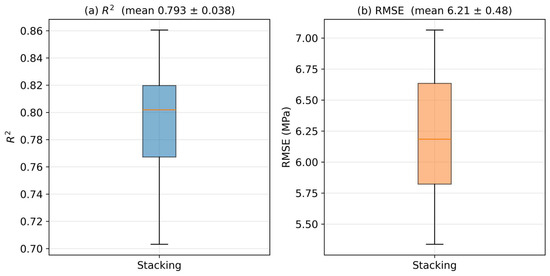
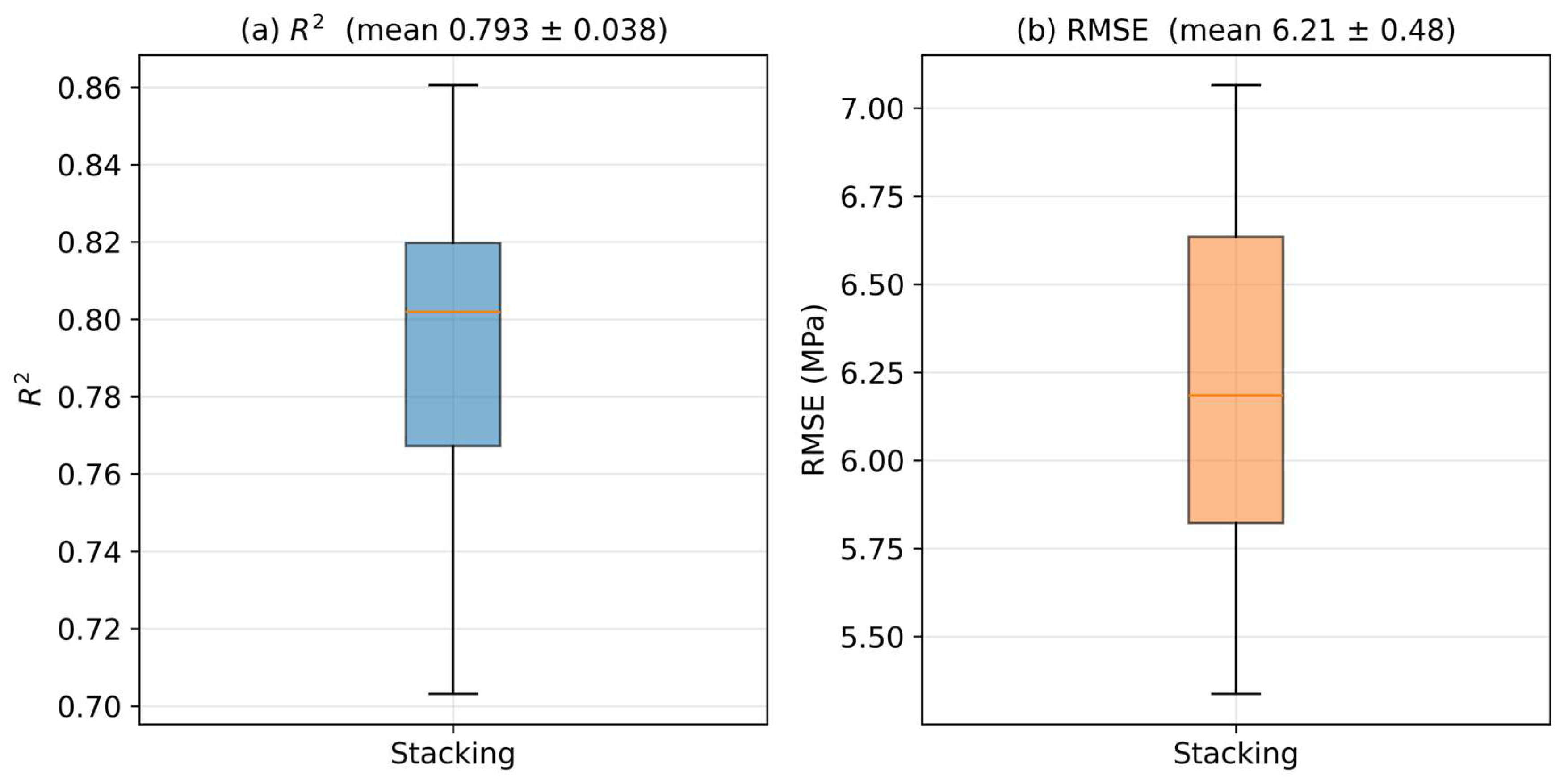
The distribution of R² and RMSE across the 25 random splits (Figure 4) shows little scatter (standard deviation of R² ≈ 0.038), meaning that performance depends only slightly on the choice of a particular split. This is an important methodological observation, since estimates based on a single split can substantially over- or under-estimate the true performance of a model. The same conclusion holds under other resampling schemes. Five-fold and ten-fold cross-validation give R² of 0.755 and 0.779, respectively, which is close to the repeated hold-out value. A stratified split by strength quartile yields 0.798 against 0.790 for the plain random split (both re-evaluated within this stratification experiment and consistent with the 0.793 obtained over all 25 splits), with the mismatch between the training and test distributions (Kolmogorov–Smirnov statistic) falling from 0.083 to 0.052. The choice of resampling protocol therefore does not change the conclusions. Table 8 collects these protocol comparisons.

Figure 4. Distribution of R² and RMSE across 25 random 70/30 splits: (a) R²; (b) RMSE.

Table 8. Comparison of resampling protocols for the proposed ensemble and a tuned single model (mean R² ± standard deviation).

Protocol	Proposed Stacking	Tuned XGBoost
25 repeated 70/30 splits	0.793 ± 0.038	0.786 ± 0.038
5-fold cross-validation (×5)	0.755 ± 0.056	0.805 ± 0.048
10-fold cross-validation (×3)	0.779 ± 0.072	0.827 ± 0.062

5.5. Predictions, Variable Importance, and Marginal Effects

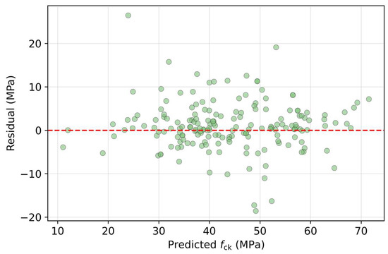
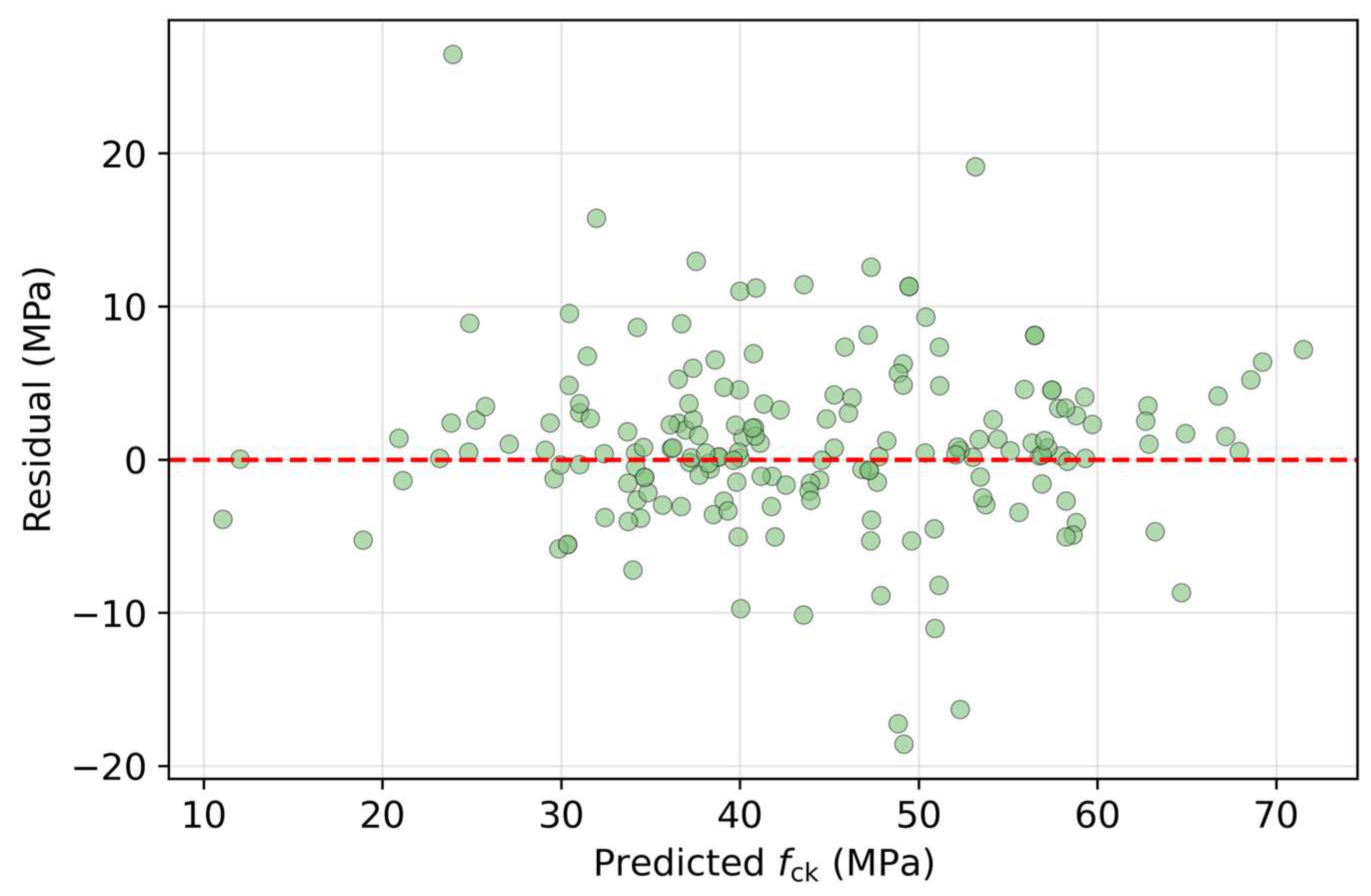
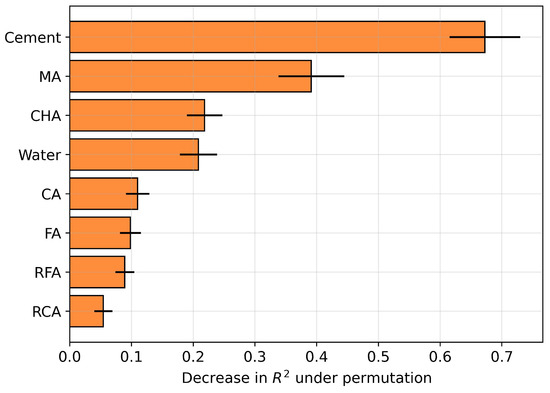
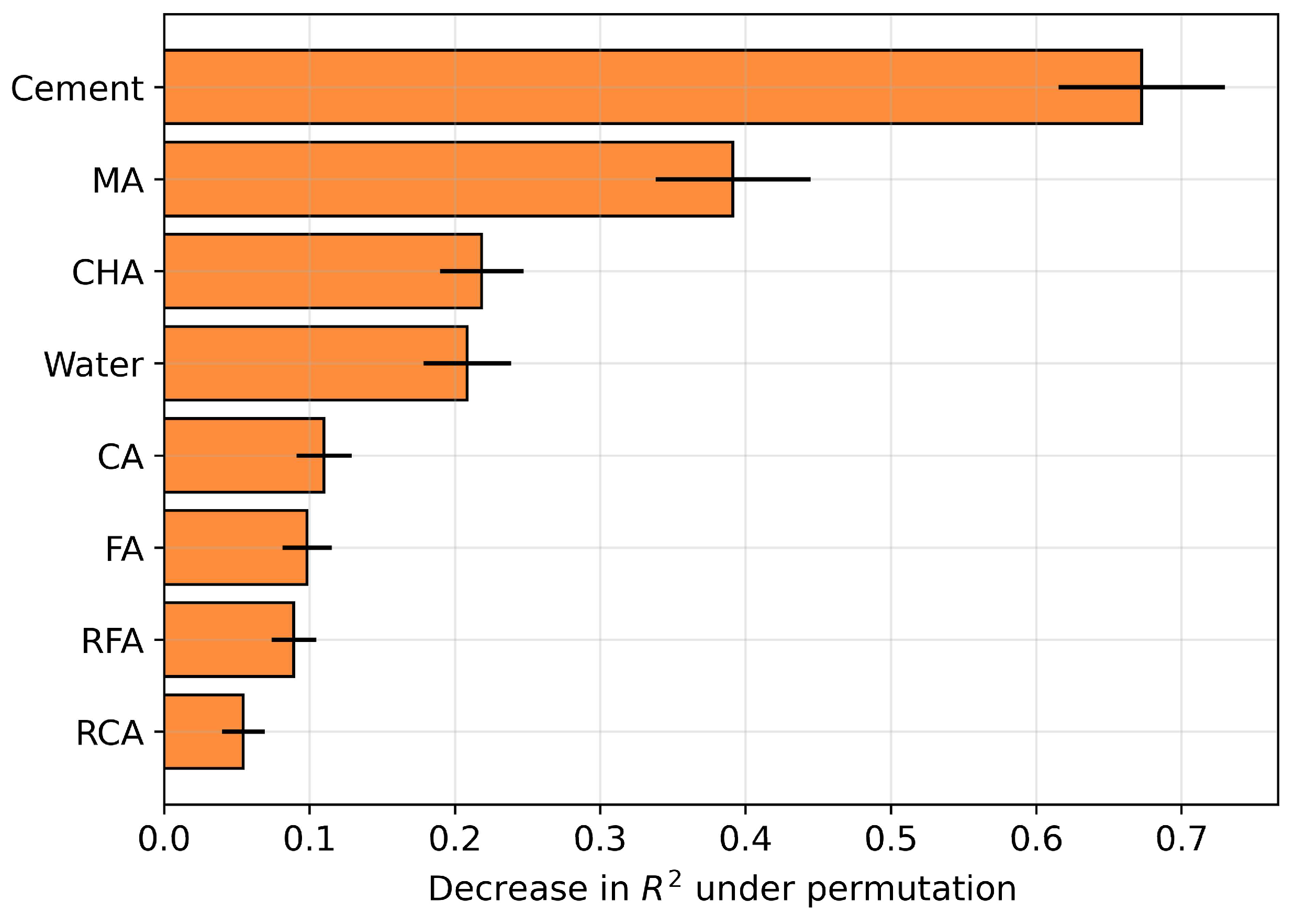
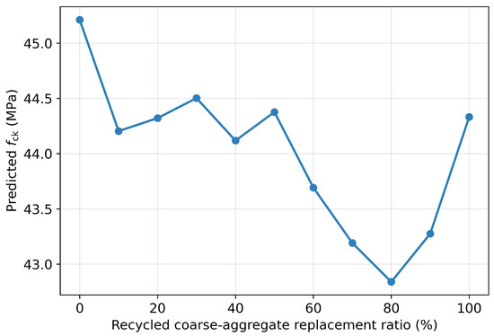
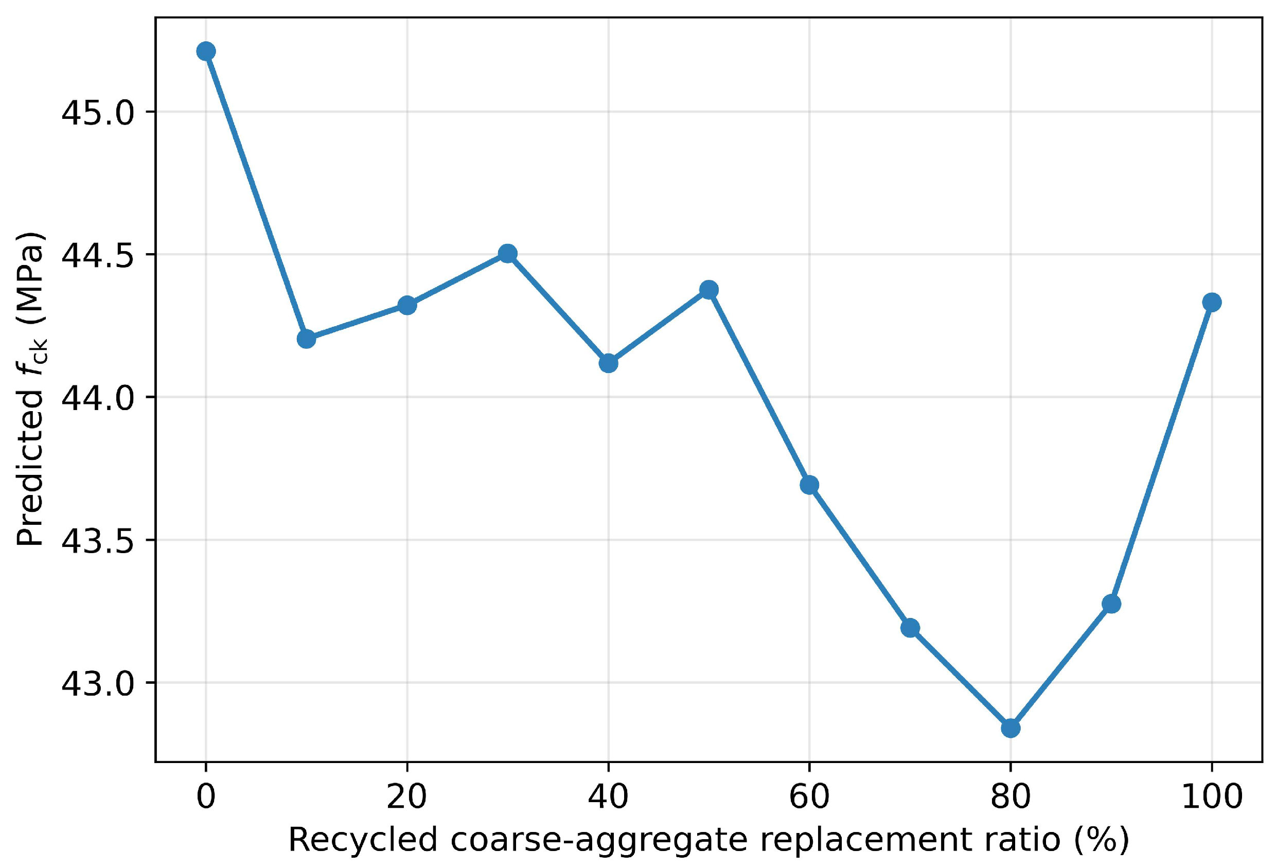
The predicted-versus-measured plot (Figure 5) shows that the points lie close to the ideal line, without pronounced systematic bias, which is confirmed by the residual distribution (Figure 6). Permutation importance (Figure 7) ranks cement first, followed by the mineral admixture, the chemical admixture, and water. The low apparent rank of water reflects the known unreliability of permutation importance under correlated inputs (Section 3) rather than a minor physical role, since water has one of the highest mutual-information scores. Partial-dependence analysis (Figure 8) confirms the physically expected directions, with strength rising as cement increases and falling as water increases, while a dedicated replacement curve (Figure 9) shows that raising the recycled-coarse-aggregate ratio lowers the predicted strength only slightly, by about 0.9 MPa across the full range. In this dataset strength is governed far more by the binder and water than by the recycled fraction itself. Variable-importance and partial-dependence analyses have become a standard part of the explainable application of machine learning, from model interpretation to feature selection [37].

Figure 5. Predicted vs. measured compressive strength (representative split). The red dashed line is the ideal 1:1 relation.

Figure 6. Residuals vs. predicted value.

Figure 7. Permutation importance of input variables. Because the inputs are correlated, this ranking should be read together with the mutual-information scores in Figure 2b.

Figure 8. Partial-dependence plots of the predicted compressive strength for the five most relevant inputs.

Figure 9. Predicted compressive strength as a function of the recycled coarse-aggregate replacement ratio, with all other components held at their median values.

5.6. Agreement with the Literature and Engineering Reliability

The obtained findings are consistent with the conclusions of recent studies reported in the literature. The trend toward tree-based ensemble methods, which stand out in the literature for their reliability and physical consistency [14,15], is in agreement with the results of the research conducted in this work. The R² and RMSE values of the proposed ensemble lie above all four reference machine-learning models. The dominance of cement and water among the predictors matches the sensitivity analyses from the literature, which consistently single out cement content and the water-to-binder ratio as the most influential strength factors [8]. As an additional measure of engineering reliability, the a20-index was computed, defined as the proportion of predictions whose ratio to the measured value deviates by less than ±20%. For the proposed model on a representative split, it is 0.87. Values of this order are interpreted in the literature as an indicator of the model’s practical usability in laboratory mix optimization [15].

5.7. Comparison with the Most Recent Work on the Same Dataset (Abood et al.)

The most recent study, by Abood et al. [22], conducted on the same dataset presented in the work of Jagadesh et al. [1], proposes a single gradient-boosting model optimized by Bayesian optimization (BO-GBRT), reporting a five-fold cross-validation R² = 0.806 (RMSE 6.00 MPa) and, on a single 90/10 split, a test R² = 0.868. For an objective comparison, the proposed ensemble was evaluated under the identical 90/10 protocol. On the reference split, the ensemble achieves R² = 0.859, close to the value of 0.868 they report in their study [22]. Across 25 random 90/10 splits, R² varies over a wide range (mean 0.844, maximum 0.911), so a value from a single split should be interpreted together with the average over multiple splits. A high training R² (0.990, close to the value of 0.989 reported by the authors [22]) indicates that both approaches share the same high-fitting regime on this dataset.

Two differences constitute the contribution of this work relative to the study by Abood et al. [22]. First, instead of a single model, a heterogeneous stacking ensemble is proposed, and performance is evaluated not on one but on 25 repeated splits, yielding a reliable, robust estimate (R² = 0.793 ± 0.038). Second, unlike the approach described in [22], data quality is explicitly addressed. The dataset contains 84 groups of identical compositions (21 of them with a contradictory measured strength), so identical compositions can “leak” between the training and test sets. Under an objective, leakage-free evaluation (merging identical compositions), the coefficient of determination drops to between 0.60 and 0.71 depending on the protocol (Section 5.2), suggesting that the reported values of about 0.81–0.87 on this dataset partly originate from the leakage of identical compositions. This observation applies to all models on the same dataset and constitutes a methodological contribution independent of the choice of model. A concise comparison under the matched protocol is given in Table 9.

Table 9. Matched-protocol comparison with Abood et al. [22] on the same dataset.

Protocol/Metric	Abood et al. [BO-GBRT]	Proposed Ensemble
Test R2 (90/10, reference split)	0.868	0.859
Test R2 (90/10, 25 splits, mean)	— (single split)	0.844 (max 0.911)
Robust R2 (70/30, 25 splits)	Not reported	0.793 ± 0.038
Train R2	0.989	0.990
Leakage-free R2 (unique compositions)	Not assessed	0.60 to 0.71

5.8. Ablation of Base Learners

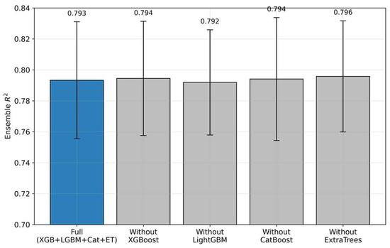
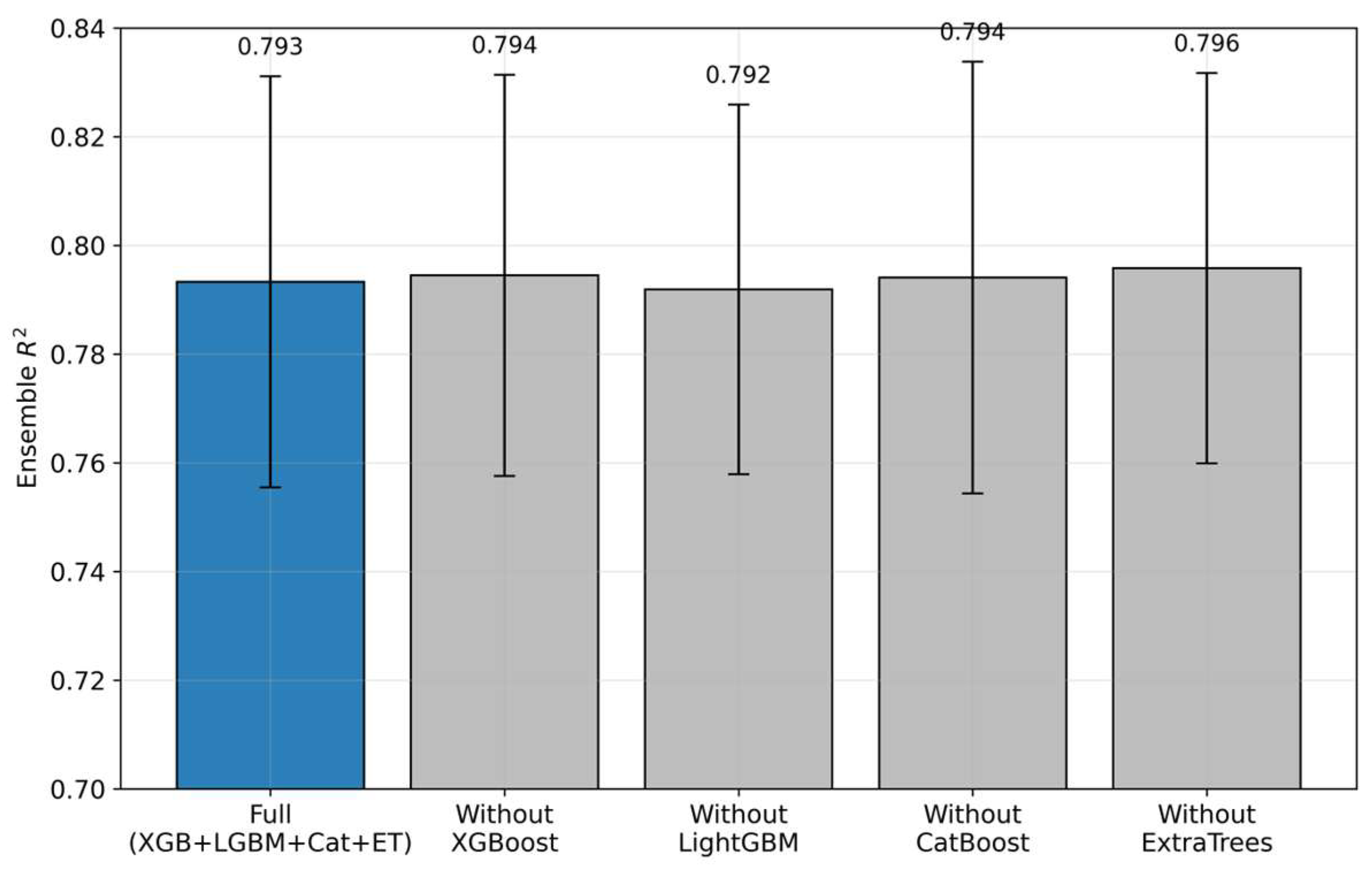
To determine the contribution of each base model, an ablation was carried out. One base model at a time is removed from the ensemble, and the performance of the remaining stacking is measured under the same repeated 70/30 protocol (25 splits). The results are given in Table 10 and shown in Figure 10.

Table 10. Ablation of base learners (leave-one-out, mean over 25 × 70/30 splits).

Ensemble Configuration	R2 (Mean over 25 × 70/30)
Full (XGB + LightGBM + CatBoost + ExtraTrees)	0.7933 ± 0.0378
Without XGBoost	0.7945 ± 0.0369
Without LightGBM	0.7919 ± 0.0340
Without CatBoost	0.7941 ± 0.0397
Without ExtraTrees	0.7958 ± 0.0359

Figure 10. Ablation analysis: ensemble R² when each base learner is removed. Error bars show the standard deviation over 25 splits.

All configurations lie within one standard deviation (≈0.79 ± 0.04), so no individual base model is decisive. The ensemble is robust to the choice of composition. Removing Extra Trees even slightly raises the mean R² (0.7958 versus 0.7933), indicating that the main contribution comes from the gradient-boosting models, while Extra Trees here acts as a mild (almost redundant) stabilizer. It is evident that the value of the ensemble lies in its stability and robustness to model choice, rather than in the necessity of all four components.

5.9. Statistical Significance and Computational Cost

To verify that the advantage of the ensemble is not due to chance, the per-split R² values were compared over the same 25 splits with the Wilcoxon signed-rank test for paired samples. Against the default reference-type models the advantage is clear and highly significant, with the ensemble winning on 22 to 25 of the 25 splits (p < 0.001 in each case). Against a carefully tuned single XGBoost the ensemble is better on 19 of 25 splits, with a mean of 0.793 versus 0.786 (p = 0.01). The difference is statistically significant but small in magnitude.

Against the default models of the reference study [1] the proposed ensemble shows a clear and consistent advantage (R² = 0.793 versus the best reference value of 0.7635). Against a carefully tuned single model the advantage shrinks to a small though still significant margin, and under the leakage-free group-aware protocol it disappears entirely, the single booster performing better (Section 5.2). The value of the proposed ensemble therefore lies not in a higher accuracy ceiling but in its stable behavior across splits and in the fact that it does not require selecting and tuning a single winning model, at the cost of greater computational complexity (training about 6.7 s versus 1.1 s for the individual XGBoost).

5.10. Diversity of Base Learners

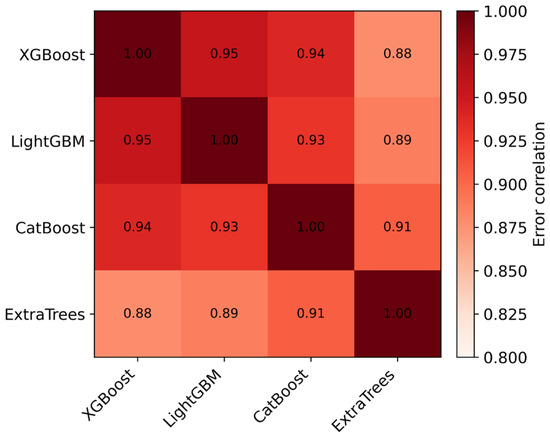
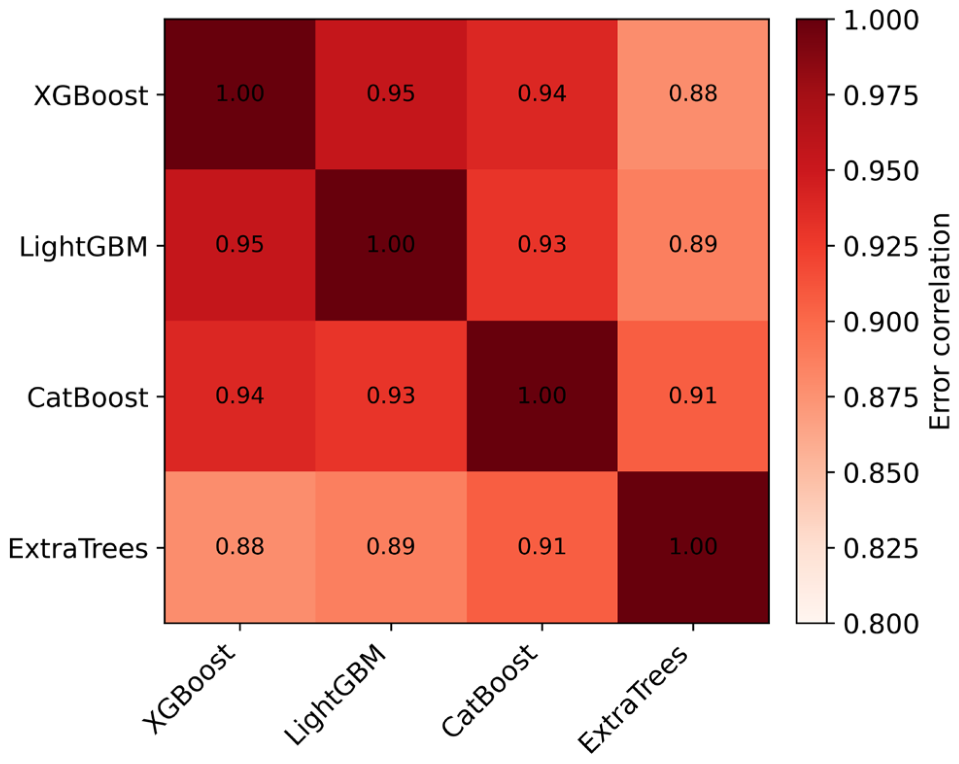
Stacking is beneficial only if the base models err in a complementary (weakly correlated) way. To examine this, the out-of-fold errors of each base model and their mutual correlation, the individual R² of each model (25 × 70/30), and the ridge meta-learner weights were computed. The individual performances and meta-weights are given in Table 11, and the correlation structure of the errors in Figure 11.

Table 11. Individual performance of base learners and their ridge meta-learner weights.

Base Learner	Individual R2 (25 × 70/30)	Ridge Meta-Weight
XGBoost	0.7877 ± 0.0379	−0.295
LightGBM	0.7932 ± 0.0393	0.275
CatBoost	0.7879 ± 0.0345	−0.053
Extra Trees	0.7600 ± 0.0399	0.919

Figure 11. Pairwise correlation of out-of-fold prediction errors between base learners (higher = more similar errors, i.e., less diversity).

The errors of the base models are highly correlated with one another (mean correlation 0.92), meaning that the models make similar errors and that the available diversity is limited. This explains why the gain of stacking over the individual model is modest, though statistically significant (Section 5.9). When predictions are highly correlated, combining them adds little. Extra Trees, as the only member of the bagging family, produces the least correlated errors (the greatest complementarity) and therefore receives the largest meta-weight (0.92), even though its individual R² is the lowest (0.760), which is consistent with the ablation, where its removal hardly changes performance. The negative and small weights of the other models reflect the high collinearity of their predictions. The analysis shows that the ensemble is stable and physically meaningful, but that the room for improvement over a single model is narrow because of the limited diversity of the base learners.

Whether this limited diversity could be improved was tested by adding two non-tree learners, a support vector regressor and a multilayer perceptron, both tuned and standardized. Individually they are considerably weaker than the boosters (R² of about 0.59 and 0.49) but, as expected, their errors are less correlated with the tree models, and the mean pairwise error correlation of the enlarged ensemble falls from 0.92 to 0.78. Even so, adding them does not improve the ensemble. The mean R² is 0.793 for the four-model base and 0.791 with both extra learners (Wilcoxon p < 0.001 against the base, in the direction of a slight decrease), because the meta-learner still relies on the accurate gradient-boosting predictions and the two weak learners add more variance than useful signal. The homogeneity of the three boosters is itself expected, since they operate on the same eight features, minimize the same squared-error loss, and share a greedy tree-growing inductive bias. A separate check confirmed that adding physically engineered features (water-to-cement and water-to-binder ratios, replacement ratios and similar) does not help either. The ensemble reaches R² = 0.789 with an enlarged set of twenty-two variables against 0.793 with the original eight variables (p = 0.37). Meaningful additional diversity on this dataset would therefore require genuinely new information rather than more learners or derived features.

5.11. Aspects in Which the Reference Study Retains an Advantage

For the sake of objectivity, the aspects in which the reference study retains an advantage are also stated. Jagadesh et al. [1] report that their artificial neural network achieves R² = 0.86 on the test set, which is higher than the R² of the proposed ensemble (0.793). Although that result comes from a single split and, in the checks carried out in this work, was not reproducible on repeated random splits, according to the published data it represents a higher reported performance. In addition, the neural network in the study by Jagadesh et al. [1] is architecturally considerably simpler (a single hidden layer with nine neurons) than the proposed ensemble of four base models. Nevertheless, if its performance were confirmed, it would represent an exceptionally compact solution. The advantage of the proposed approach therefore lies not in simplicity but in its proven robustness and its consistent outperformance of reproducible models.

5.12. Limitations

The dataset is relatively small (603 mixtures) and collected from heterogeneous sources, contains extreme values of some admixtures, and the conclusions are limited to the range of compositions represented in the data. The stacking ensemble is also computationally more demanding than a single model, which is the price of greater stability. A more fundamental limitation, made explicit by the analyses above, is generalization. Under leakage-free and especially cross-source evaluation, the accuracy is substantially lower than the headline figure, so the model should be regarded as a screening tool within the represented composition space rather than a validated predictor for new sources. External laboratory validation on independently produced mixtures remains necessary and is left for future work.

6. Conclusions

This work re-examined machine-learning prediction of the compressive strength of self-compacting concrete with recycled coarse aggregate on a widely used benchmark, using a heterogeneous stacking ensemble as a representative model. Averaged over 25 repeated 70/30 splits, the ensemble reaches R² = 0.793 ± 0.038 and RMSE = 6.21 ± 0.48 MPa, above all four machine-learning models of the reference study and, by a small but significant margin, above a tuned single booster. Its main value, however, is stability rather than a higher ceiling: an ablation shows no base model to be decisive, the base learners are highly correlated (mean error correlation 0.92), and adding support-vector, multilayer-perceptron, or engineered-feature diversity does not improve the result. The most important findings concern evaluation. Because the 603 rows contain only 504 unique compositions, a leakage-free protocol lowers the R² of every model to between 0.60 and 0.71, and leave-one-source-out evaluation lowers it to about 0.14; the accuracies of roughly 0.81–0.87 previously reported on this dataset are therefore substantially inflated by duplicate-composition leakage. Mutual-information and partial-dependence analyses give the model a physically consistent interpretation, with cement dominant and water acting through a nonlinear dependence, while a single extreme admixture value was shown not to affect the results.

Several directions follow from these findings. The most pressing is external validation on independently produced mixtures and, where possible, richer composition descriptors, since cross-source generalization is the weakest point identified here. Methodologically, leakage-aware and cross-source evaluation should become standard when models are compared on pooled literature datasets, so that reported gains are not artifacts of repeated records. Further work could explore uncertainty quantification such as conformal prediction intervals, deep tabular architectures, and extension to other properties of self-compacting recycled-aggregate concrete, such as workability and durability, as well as deployment as an openly available screening tool. More broadly, the study supports the recent trend [8,14] toward tree-based ensembles as reliable and interpretable models for this problem, while cautioning that their reported accuracy must be established under leakage-free evaluation.

References

- Jagadesh, P.; Khan, A.H.; Priya, B.S.; Asheeka, A.; Zoubir, Z.; Magbool, H.M.; Alam, S.; Bakather, O.Y. Artificial Neural Network, Machine Learning Modelling of Compressive Strength of Recycled Coarse Aggregate Based Self-Compacting Concrete. PLoS ONE 2024, 19, e0303101. [Google Scholar] [CrossRef] [Scilit] [PubMed]
- Duan, Z.H.; Kou, S.C.; Poon, C.S. Prediction of Compressive Strength of Recycled Aggregate Concrete Using Artificial Neural Networks. Constr. Build. Mater. 2013, 40, 1200–1206. [Google Scholar] [CrossRef] [Scilit]
- Suescum-Morales, D.; Salas-Morera, L.; Jiménez, J.R.; García-Hernández, L. A Novel Artificial Neural Network to Predict Compressive Strength of Recycled Aggregate Concrete. Appl. Sci. 2021, 11, 11077. [Google Scholar] [CrossRef] [Scilit]
- Nguyen, T.-D.; Cherif, R.; Mahieux, P.-Y.; Lux, J.; Aït-Mokhtar, A.; Bastidas-Arteaga, E. Artificial Intelligence Algorithms for Prediction and Sensitivity Analysis of Mechanical Properties of Recycled Aggregate Concrete: A Review. J. Build. Eng. 2023, 66, 105929. [Google Scholar] [CrossRef] [Scilit]
- Concu, G.; Zucca, M.; Stochino, F.; Valdés, M.; Maltinti, F. The Use of Perlite and Rhyolite in Concrete Mix Design: Influence on Physical-Mechanical and Environmental Performance. Technologies 2025, 13, 224. [Google Scholar] [CrossRef] [Scilit]
- Boudali, S.; Abdulsalam, B.; Rafiean, A.H.; Poncet, S.; Soliman, A.; ElSafty, A. Influence of Fine Recycled Concrete Powder on the Compressive Strength of Self-Compacting Concrete (SCC) Using Artificial Neural Network. Sustainability 2021, 13, 3111. [Google Scholar] [CrossRef] [Scilit]
- de-Prado-Gil, J.; Palencia, C.; Jagadesh, P.; Martínez-García, R. A Study on the Prediction of Compressive Strength of Self-Compacting Recycled Aggregate Concrete Utilizing Novel Computational Approaches. Materials 2022, 15, 5232. [Google Scholar] [CrossRef] [Scilit] [PubMed]
- Almutairi, A. Explainable Machine Learning-Based Prediction of Compressive Strength in Sustainable Recycled Aggregate Self-Compacting Concrete Using SHAP Analysis. Sustainability 2025, 17, 11334. [Google Scholar] [CrossRef] [Scilit]
- Alyaseen, A.; Poddar, A.; Kumar, N.; Tajjour, S.; Prasad, C.V.S.R.; Alahmad, H.; Sihag, P. High-Performance Self-Compacting Concrete with Recycled Coarse Aggregate: Soft-Computing Analysis of Compressive Strength. J. Build. Eng. 2023, 77, 107527. [Google Scholar] [CrossRef] [Scilit]
- Mitikie, B.B.; Elsaigh, W.A. AI-Driven Bibliometric Analysis of Bacterial Concrete Research (2020–2025). Technologies 2026, 14, 340. [Google Scholar] [CrossRef] [Scilit]
- Bolandi, H.; Banzhaf, W.; Lajnef, N.; Barri, K.; Alavi, A.H. An Intelligent Model for the Prediction of Bond Strength of FRP Bars in Concrete: A Soft Computing Approach. Technologies 2019, 7, 42. [Google Scholar] [CrossRef] [Scilit]
- Nikmehr, B.; Kafle, B.; Al-Ameri, R. Performance Assessment of One-Part Self-Compacted Geopolymer Concrete Containing Recycled Concrete Aggregate: A Critical Comparison Using Artificial Neural Network (ANN) and Linear Regression Models. Recycling 2024, 9, 73. [Google Scholar] [CrossRef] [Scilit]
- de-Prado-Gil, J.; Martínez-García, R.; Jagadesh, P.; Juan-Valdés, A.; González-Alonso, M.-I.; Palencia, C. To Determine the Compressive Strength of Self-Compacting Recycled Aggregate Concrete Using Artificial Neural Network (ANN). Ain Shams Eng. J. 2024, 15, 102548. [Google Scholar] [CrossRef] [Scilit]
- Yang, S.; Sun, J.; Xu, Z. Prediction on Compressive Strength of Recycled Aggregate Self-Compacting Concrete by Machine Learning Method. J. Build. Eng. 2024, 88, 109055. [Google Scholar] [CrossRef] [Scilit]
- Yang, S.; Chen, T.; Xu, Z. Estimation on Compressive Strength of Recycled Aggregate Self-Compacting Concrete Using Interpretable Machine Learning-Based Models. Eng. Comput. 2024, 41, 2727–2773. [Google Scholar] [CrossRef] [Scilit]
- Zhang, J.; Wang, Z.; Shen, S.; Sheng, S.; He, H.; He, C. Hybrid Explainable Machine Learning Models with Metaheuristic Optimization for Performance Prediction of Self-Compacting Concrete. Buildings 2026, 16, 225. [Google Scholar] [CrossRef] [Scilit]
- Khan, M.F.; Javed, M.F.; Alabduljabbar, H.; Ahmad, F. Explainable Machine Learning and Ensemble Models for Predicting Fresh Properties of Self-Consolidating Concrete. Sci. Rep. 2025, 15, 42288. [Google Scholar] [CrossRef] [Scilit] [PubMed]
- Awoyera, P.O.; Simwanda, L.; Vasić, M.V.; Mydin, M.A.O.; Imoh, U.U.; Fadugba, O.G.; Asiz, A.; Movahedi Rad, M. Hybrid Generative–Ensemble Approach for Predicting Recycled Aggregate Concrete Strength Properties. Sci. Rep. 2026, 16, 15205. [Google Scholar] [CrossRef] [Scilit] [PubMed]
- Imani, M.; Beikmohammadi, A.; Arabnia, H.R. Comprehensive Analysis of Random Forest and XGBoost Performance with SMOTE, ADASYN, and GNUS Under Varying Imbalance Levels. Technologies 2025, 13, 88. [Google Scholar] [CrossRef] [Scilit]
- Yu, Y.; Al-Damad, I.M.A.; Foster, S.J.; Nezhad, A.A.; Hajimohammadi, A. Compressive Strength Prediction of Fly Ash/Slag-Based Geopolymer Concrete Using EBA-Optimised Chemistry-Informed Interpretable Deep Learning Model. Dev. Built Environ. 2025, 23, 100736. [Google Scholar] [CrossRef] [Scilit]
- Yu, Y.; Jayathilakage, R.; Liu, Y.; Hajimohammadi, A. Intelligent Compressive Strength Prediction of Sustainable Rubberised Concrete Using an Optimised Interpretable Deep CNN-LSTM Model with Attention Mechanism. Appl. Soft Comput. 2025, 185, 113993. [Google Scholar] [CrossRef] [Scilit]
- Abood, E.A.; Thoeny, Z.A.; Azize, N.M.; Imran, H.; Kamchoom, V.; Onyelowe, K.C.; Arunachalam, K.P. Self Compacting Concrete with Recycled Aggregate Compressive Strength Prediction Based on Gradient Boosting Regression Tree with Bayesian Optimization Hybrid Model. Sci. Rep. 2025, 15, 28175. [Google Scholar] [CrossRef] [Scilit] [PubMed]
- Dong, S.; Zhang, Z. Hybrid Deep Learning with Conformal Prediction for Recycled Aggregate Self-Compacting Concrete Strength Prediction. Buildings 2025, 15, 4419. [Google Scholar] [CrossRef] [Scilit]
- Breiman, L.; Friedman, J.H.; Olshen, R.A.; Stone, C.J. Classification and Regression Trees; Wadsworth: Belmont, CA, USA, 1984. [Google Scholar]
- Breiman, L. Bagging Predictors. Mach. Learn. 1996, 24, 123–140. [Google Scholar] [CrossRef] [Scilit]
- Breiman, L. Random Forests. Mach. Learn. 2001, 45, 5–32. [Google Scholar] [CrossRef] [Scilit]
- Geurts, P.; Ernst, D.; Wehenkel, L. Extremely Randomized Trees. Mach. Learn. 2006, 63, 3–42. [Google Scholar] [CrossRef] [Scilit]
- Friedman, J.H. Greedy Function Approximation: A Gradient Boosting Machine. Ann. Stat. 2001, 29, 1189–1232. [Google Scholar] [CrossRef] [Scilit]
- Chen, T.; Guestrin, C. XGBoost: A Scalable Tree Boosting System. In Proceedings of the 22nd ACM SIGKDD International Conference on Knowledge Discovery and Data Mining, San Francisco, CA, USA, 13–17 August 2016; pp. 785–794. [Google Scholar]
- Ke, G.; Meng, Q.; Finley, T.; Wang, T.; Chen, W.; Ma, W.; Ye, Q.; Liu, T.-Y. LightGBM: A Highly Efficient Gradient Boosting Decision Tree. In Advances in Neural Information Processing Systems 30; Curran Associates: Red Hook, NY, USA, 2017; pp. 3146–3154. [Google Scholar]
- Prokhorenkova, L.; Gusev, G.; Vorobev, A.; Dorogush, A.V.; Gulin, A. CatBoost: Unbiased Boosting with Categorical Features. In Advances in Neural Information Processing Systems 31; Curran Associates: Red Hook, NY, USA, 2018; pp. 6638–6648. [Google Scholar]
- Wolpert, D.H. Stacked Generalization. Neural Netw. 1992, 5, 241–259. [Google Scholar] [CrossRef] [Scilit]
- Hoerl, A.E.; Kennard, R.W. Ridge Regression: Biased Estimation for Nonorthogonal Problems. Technometrics 1970, 12, 55–67. [Google Scholar] [CrossRef]
- Tan, T.-H.; Chen, G.-H.; Liu, S.-H.; Chen, W. Prediction of Sleep Apnea Occurrence from a Single-Lead Electrocardiogram Using Stacking Hybrid Architecture with Gated Recurrent Neural Network Architectures and Logistic Regression. Technologies 2026, 14, 92. [Google Scholar] [CrossRef] [Scilit]
- Akiba, T.; Sano, S.; Yanase, T.; Ohta, T.; Koyama, M. Optuna: A Next-Generation Hyperparameter Optimization Framework. In Proceedings of the 25th ACM SIGKDD International Conference on Knowledge Discovery and Data Mining, Anchorage, AK, USA, 4–8 August 2019; pp. 2623–2631. [Google Scholar]
- Pedregosa, F.; Varoquaux, G.; Gramfort, A.; Michel, V.; Thirion, B.; Grisel, O.; Blondel, M.; Prettenhofer, P.; Weiss, R.; Dubourg, V.; et al. Scikit-Learn: Machine Learning in Python. J. Mach. Learn. Res. 2011, 12, 2825–2830. [Google Scholar]
- Al-Shourbaji, I.; Alameen, A. Optimizing Solar Radiation Prediction with ANN and Explainable AI-Based Feature Selection. Technologies 2025, 13, 263. [Google Scholar] [CrossRef] [Scilit]
Disclaimer/Publisher’s Note: The statements, opinions and data contained in all publications are solely those of the individual author(s) and contributor(s) and not of MDPI and/or the editor(s). MDPI and/or the editor(s) disclaim responsibility for any injury to people or property resulting from any ideas, methods, instructions or products referred to in the content. |
© 2026 by the authors. Licensee MDPI, Basel, Switzerland. This article is an open access article distributed under the terms and conditions of the Creative Commons Attribution (CC BY) license.