Research on Underwater Robot Control Method Based on PSO-RBF-Optimized PID

Abstract

To address the limitations of traditional controllers for the considered six-degree-of-freedom multi-thruster underwater robot under strong nonlinearities and environmental disturbances, this paper proposes a particle swarm optimization–radial basis function–proportional–integral–derivative (PSO-RBF-PID) control algorithm. The proposed method combines the nonlinear identification capability of the RBF neural network, the global optimization capability of PSO, and the stable closed-loop structure of PID control, thereby enabling adaptive parameter tuning and disturbance compensation. Unlike existing PSO-PID- and RBF-based controllers, the proposed method combines offline global optimization and online adaptive gain tuning within a unified control framework. Although the framework is modular and can be extended to underwater robotic systems with different degrees of freedom by redefining the state vector, controller channels, and thrust allocation matrix, the present study validates the method through a six-degree-of-freedom multi-thruster underwater robot case study. Comparative simulations were conducted under the same model, disturbance conditions, sampling settings, and evaluation indices for six controllers: PID, cascade PID, fuzzy PID, FOPID, PSO-PID, and PSO-RBF-PID. For the considered 6-DOF multi-thruster underwater robot, PSO-RBF-PID achieved the best overall performance in steady-state error, settling time, overshoot, and IAE. This improvement is mainly attributed to the combination of PSO-based offline optimization and RBF-based online adaptive compensation.

1. Introduction

Underwater robots are widely used in ocean exploration and environmental monitoring, but their control is challenged by strong nonlinear dynamics, external disturbances, and model uncertainties.

To address these issues, various control strategies have been developed, including PID, fuzzy PID, and optimization-based methods. PID controllers are widely used due to their simplicity, whereas fuzzy logic enhances adaptability [1,2]. Optimization algorithms such as particle swarm optimization (PSO) further enhance parameter tuning performance. However, most existing approaches rely on single-strategy optimization and lack effective integration of multiple techniques, limiting their performance under complex conditions [3,4].

Recently, reinforcement learning (RL)-based methods have shown promising adaptability and data-driven decision-making capabilities in complex robotic control tasks [5]. For example, recent work has used reinforcement-learning-based adaptive PID control to improve the robustness of underwater vehicle depth control under buoyancy variations, highlighting the potential of RL in addressing nonlinear and disturbance-rich environments [6]. By continuously interacting with the environment, RL can enhance the autonomy and robustness of underwater systems, effectively addressing challenges such as nonlinear dynamics, model uncertainties, and external disturbances [7]. Similarly, safe reinforcement learning integrated with active disturbance rejection has been explored for autonomous navigation to improve the tracking and disturbance robustness of UUVs [8]. Through this iterative learning process, RL enables these systems to adapt to varying conditions and improve performance in dynamic underwater environments [9].

However, its practical application is still limited by high computational cost, large training-data requirements, complex reward-function design, and the simulation-to-reality gap [10,11]. Therefore, a computationally efficient control strategy with adaptive learning capability remains necessary for practical underwater robot applications.

To overcome these limitations, this paper proposes a hybrid particle swarm optimization–radial basis function–proportional–integral–derivative (PSO-RBF-PID) control framework. PSO is used offline to optimize RBF network parameters and initial PID gains, while the RBF network performs online adaptive tuning to compensate for uncertainties and disturbances [12,13]. A comprehensive comparative evaluation with multiple benchmark controllers is conducted to validate the effectiveness of the proposed method under consistent simulation conditions.

Fractional-order PID (FOPID) controllers provide greater tuning flexibility than conventional PID controllers by introducing adjustable integral and derivative orders and have demonstrated improved performance in some applications [14]. However, their implementation typically requires fractional-order approximation, leading to increased computational complexity. In this study, FOPID is used as a benchmark controller. Unlike FOPID, the proposed PSO-RBF-PID improves adaptability through PSO-based parameter optimization and RBF-based online gain adjustment without introducing fractional-order operators.

The main contributions of this paper are summarized as follows:

• A hybrid PSO-RBF-PID control framework is proposed, in which PSO is employed to simultaneously optimize the RBF network parameters and initial PID gains. This differs from conventional approaches that optimize PID parameters alone, enabling improved global search capability and avoiding local optima [15,16].
• An RBF neural network-based adaptive mechanism is developed for online tuning of PID parameters. The network with optimized centers, widths, and weights provides effective nonlinear approximation and real-time compensation for system uncertainties and disturbances [17,18].
• A comprehensive comparative evaluation framework is established by incorporating multiple benchmark controllers, including conventional PID, fuzzy PID, cascade PID, Fractional Order PID (FOPID), and PSO-PID. Through trajectory tracking tasks and quantitative performance indices, the proposed method is systematically validated in terms of accuracy, response speed, and disturbance rejection capability [19,20].

The proposed PSO-RBF-PID method is not a standalone metaheuristic optimizer. Unlike GA-based methods that mainly perform offline parameter search through selection [21], crossover, and mutation, the proposed framework combines offline PSO-based global optimization with online RBF-based adaptive tuning and PID closed-loop feedback. PSO is used to obtain suitable initial PID gains and RBF parameters, while the RBF network continuously adjusts the PID gains according to the tracking error and system response. Therefore, the main advantage of the proposed method lies in its integration of global optimization, nonlinear approximation, and real-time adaptive feedback for disturbance rejection in underwater robot control.

The remainder of this paper is organized as follows. Section 2 presents the kinematic and dynamic models of the 6-DOF multi-thruster underwater robot, including thrust allocation and disturbance modeling. Section 3 describes the proposed PSO-RBF-PID controller and its optimization procedure. Section 4 presents the simulation setup and compares six controllers through step-response and helical trajectory-tracking tasks. Section 5 summarizes the main findings, limitations, and future work.

2. Modeling of Six-Degree-of-Freedom Underwater Robot

This section establishes the control-oriented model used for the subsequent PSO-RBF-PID controller design. Section 2.1 defines the coordinate systems and thruster layout, which determine the motion description and thrust mapping. Section 2.2 introduces the kinematic variables, Section 2.3 formulates the nonlinear dynamic model, and Section 2.4 describes the thrust allocation and disturbance model. These subsections together provide the controlled plant, feedback variables, actuator mapping, and disturbance conditions required for controller optimization and simulation.

2.1. Coordinate System and Thruster Layout

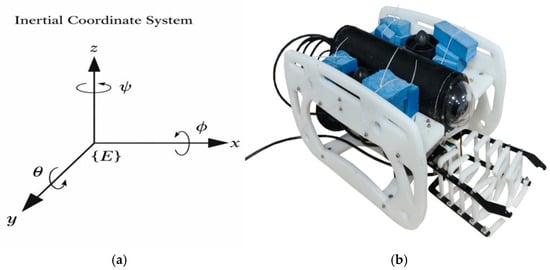
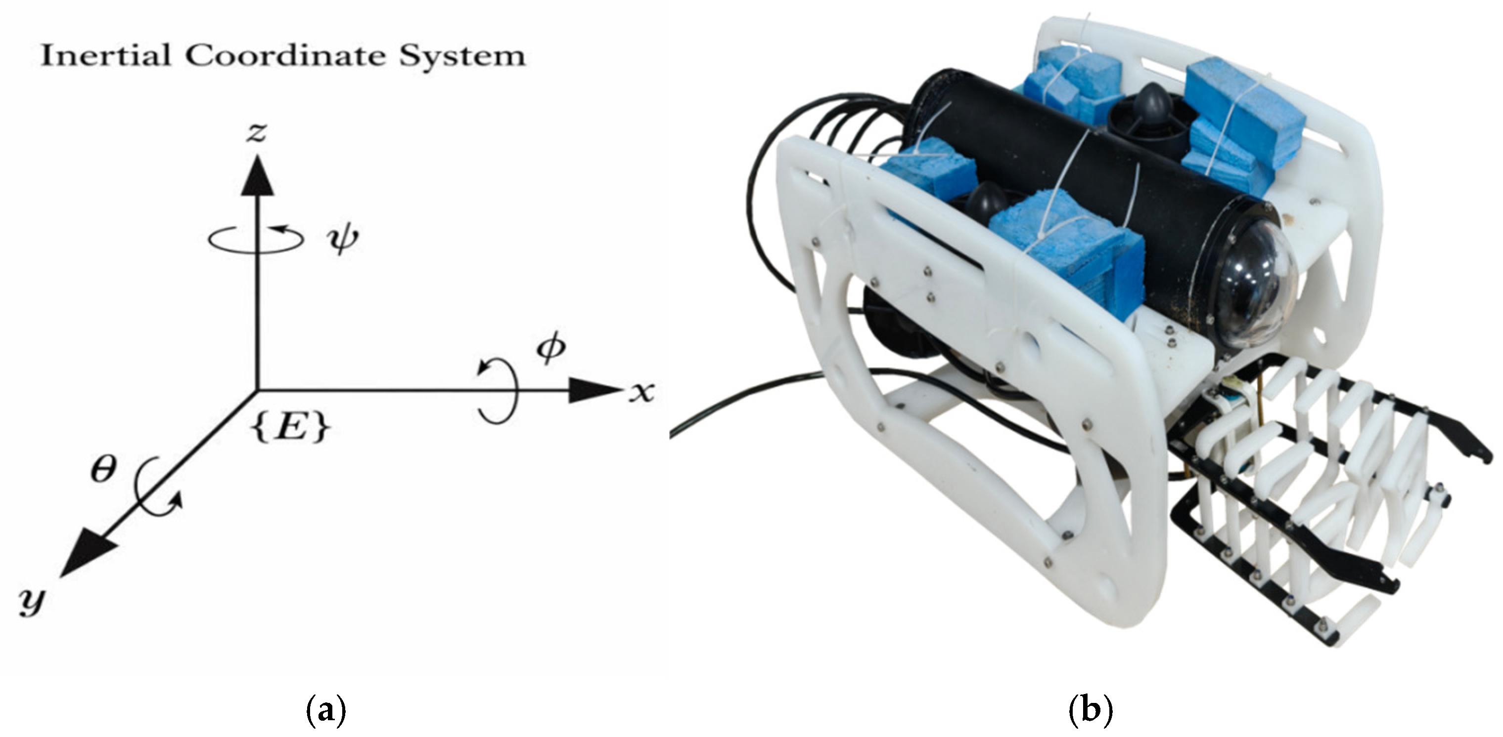
The coordinate system recommended by the International Towing Tank Conference (ITTC) and the Society of Naval Architects and Marine Engineers (SNAME) is adopted to establish two types of coordinate systems for describing the motion state of the robot [19,20]. The coordinate system and physical model of the underwater robot are shown in Figure 1.

Figure 1. Coordinate system of underwater robot (a) and model (b).

The inertial coordinate system {I} (fixed frame): Its origin is fixed on the Earth’s surface, with x-axis north, y-axis east, and z-axis downward (following marine engineering practices), used to characterize the robot’s absolute position (x, y, z) and attitude (roll angle φ, pitch angle θ, yaw angle ψ). The body coordinate system {B} (moving frame): Its origin coincides with the robot’s center of gravity, with x-axis as the longitudinal (forward) axis, y-axis as the transverse (lateral) axis, and z-axis as the vertical (downward positive) axis, used to describe the relative motion velocity (ν) and acceleration ($\dot{\nu }$).

An omnidirectional layout with six degrees of freedom is used for the thrusters. Four horizontal thrusters handle planar motion (forward/backward, lateral movement, course adjustment), and two vertical thrusters manage vertical motion (diving/floating) and attitude stabilization (roll and pitch suppression). This ensures the robot’s flexible movement in 3D space.

The thruster layout directly determines the thrust allocation matrix (B), which maps the individual thruster outputs to the generalized force/moment vector ($\tau$). Therefore, the coordinate system and thruster configuration provide the physical basis for the subsequent dynamic model and controller input allocation.

2.2. Kinematic Model

The motion state of the robot is described by three vectors.

The position–attitude vector is defined as (η = [x, y, z, φ, θ, ψ]^T), where (x, y, z) denote the position in the inertial frame and (φ, θ, ψ) denote roll, pitch, and yaw angles, respectively.

The velocity vector is defined as (ν = [u, v, w, p, q, r]^T), where (u, v, w) are the translational velocities and (p, q, r) are the angular velocities in the body-fixed frame.

The acceleration vector is defined as (ν = [du, dv, dw, dp, dq, dr]^T).

The key model parameters are introduced at their first occurrence in the following dynamic model section to make the formulation self-contained.

2.3. Dynamic Model

Based on the Newton–Euler equation and hydrodynamic theory, considering the inertial effect, fluid damping, gravity-buoyancy coupling and external disturbances during the motion of the underwater robot, the core equation of the simplified dynamic model is established [22]:

$$M\left(\nu \right)\dot{\nu }+C\left(\nu \right)\nu +D\left(\nu \right)\nu +g\left(\eta \right)={\tau }_P+{\tau }_d$$

(1)

where (M) is the total inertia matrix including rigid-body inertia and added mass; ($C\left(\nu \right)$) is the Coriolis and centripetal matrix; $D\left(\nu \right)$ is the hydrodynamic damping matrix including linear and nonlinear damping terms; $g\left(\eta \right)$ is the restoring force/moment vector induced by gravity and buoyancy; ${\tau }_P$ is the control force/moment generated by the thrusters; and ${\tau }_d$ denotes the lumped disturbance term, including ocean-current disturbance, parameter uncertainty, and unmodeled dynamics.

The definitions and nominal values/ranges of the main model parameters used in the dynamic model and simulations are summarized in Table 1. The basic physical parameters were determined according to the robot design and typical small-to-medium-sized underwater robot configurations. The hydrodynamic coefficients were estimated using simplified hydrodynamic theory and representative values from the literature. The ranges of the hydrodynamic parameters indicate the uncertainty intervals used in the robustness simulations [22].

Table 1. Definitions and nominal values/ranges of the model parameters used in the dynamic model.

Parameter Name	Symbol	Physical Meaning	Parameter Value	Selection Method
Gravitational acceleration	G	Gravitational acceleration	9.81 m/s2	Standard value
Basic physical parameters	m, Ixx, Iyy, Izz	Mass and inertia	m = 50 kg; Ixx = 2.5/Iyy = 3.0/Izz = 4.2 kg m2	Theoretical design + physical reference
Added mass coefficients	${\mathrm{X}}_{\dot{\mathrm{u}}},{\mathrm{Y}}_{\dot{\mathrm{v}}},{\mathrm{Z}}_{\dot{\mathrm{w}}},$ ${\mathrm{K}}_{\dot{\mathrm{p}}},{\mathrm{M}}_{\dot{\mathrm{q}}},{\mathrm{N}}_{\dot{\mathrm{r}}}$	Added mass coefficients	0.5 kg~12 kg; 0.5 kg·m2~0.8 kg·m2	Estimation + physical reference
Coriolis force coefficients	Cuv, Cuw, Cvw, Cpq	Coriolis coupling	0.03 kg m/s~0.08 kg/s	Estimation + physical reference
Damping coefficients	Xu, Yv, Zw, Kp, Mq, Nr, Xuu, Yvv, Zww	Damping (linear & nonlinear)	Linear: 0.05~0.15 N·s/m; Quadratic: 0.02~0.04 N s2/m2	Model-based + physical reference
Gravity–buoyancy parameters	G-B, xb, yb	Restoring force parameters	G-B = 5 N; xb = 0.02 m; yb = 0.01 m	Theoretical design

The environmental disturbance parameters are introduced in Section 2.4 when the disturbance model is formulated, while the PSO and RBF optimization parameters are defined in Section 3 when the control algorithm is presented [23].

2.4. Thrust Allocation and Disturbance Modeling

2.4.1. Thrust Allocation

The Moore–Penrose pseudo-inverse method is adopted to realize the optimal allocation of thrust, and the core logic is to convert the desired control force/moment $\tau$ into the actual thrust output of each thruster [23,24]. By establishing the thruster configuration matrix B to describe the contribution coefficient of each thruster to each degree of freedom, the optimal thrust allocation scheme is solved by pseudo-inverse operation, and the thrust output is ensured not to exceed the maximum load capacity of the thrusters through hardware limiting, thus guaranteeing the engineering feasibility of control commands.

2.4.2. Hydrodynamic Disturbance Modeling

The influence of ocean currents on the robot motion is considered by introducing a steady current in the inertial frame and transforming it into the body-fixed frame to obtain the relative velocity. Based on hydrodynamic principles, the disturbance force and moment induced by ocean currents, together with parameter perturbations and unmodeled dynamics, are integrated into a composite disturbance term ${\tau }_d$ in the dynamic model [25].

To evaluate robustness, the disturbance is modeled as a combination of constant, time-varying, and sudden components:

$$\begin{array}{c}{\tau }_d\left(t\right)={\tau }_0+A\mathit{sin}(\omega t)+{\tau }_s(t)\end{array}$$

(2)

$$\begin{array}{c}{\tau }_s\left(t\right)=\left\{\begin{array}{ll}0,& t<t_0\\ {\tau }_1,& t\ge t_0\end{array}\right.\end{array}$$

(3)

This composite disturbance represents realistic ocean conditions and enables comprehensive evaluation of disturbance rejection and recovery performance.

2.5. Model Role in Controller Optimization and Benchmark Evaluation

The physical and hydrodynamic parameters in the above model are used to construct the nonlinear controlled plant and disturbance environment. They are not directly optimized by PSO. In the proposed PSO-RBF-PID framework, the optimized variables are controller-related parameters, including the initial PID gains ($K_p$, $K_i$, $K_d$) and the RBF neural network parameters, namely the centers, widths, and output weights. During optimization, each candidate particle is applied to the closed-loop model, and the resulting tracking error and control effort are used to calculate the fitness value.

Compared with simplified single-degree-of-freedom or planar underwater robot models, the present model retains six-degree-of-freedom motion coupling, thrust allocation, hydrodynamic disturbance, actuator constraints, and parameter uncertainty. Therefore, it provides a more comprehensive benchmark for evaluating the tracking accuracy, robustness, and adaptability of the proposed PSO-RBF-PID controller.

3. Design of PSO-RBF-PID Control Algorithm

3.1. Proposed PSO-RBF-PID Controller Structure

To address the challenges of strong nonlinearity, multi-degree-of-freedom coupling, and disturbances in 6-DOF (6-Degree-of-Freedom) multi-thruster underwater robots, PSO-RBF-PID controllers are developed. By combining the global optimization capability of PSO with the nonlinear mapping of the RBF neural network, the proposed method enhances parameter adaptability and mitigates local optimum issues of conventional approaches.

The proposed architecture is modular and can be extended to underwater robots with different degrees of freedom by redefining the state vector, control input, RBF structure, thrust allocation matrix, and PSO particle dimension. However, this study only validates the method on a 6-DOF multi-thruster underwater robot, and applications to other platforms or real underwater robots require further investigation.

This section outlines the principles of PSO, the design of the PSO-RBF-PID controller, and the collaborative optimization mechanism.

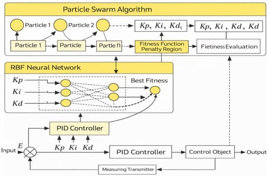
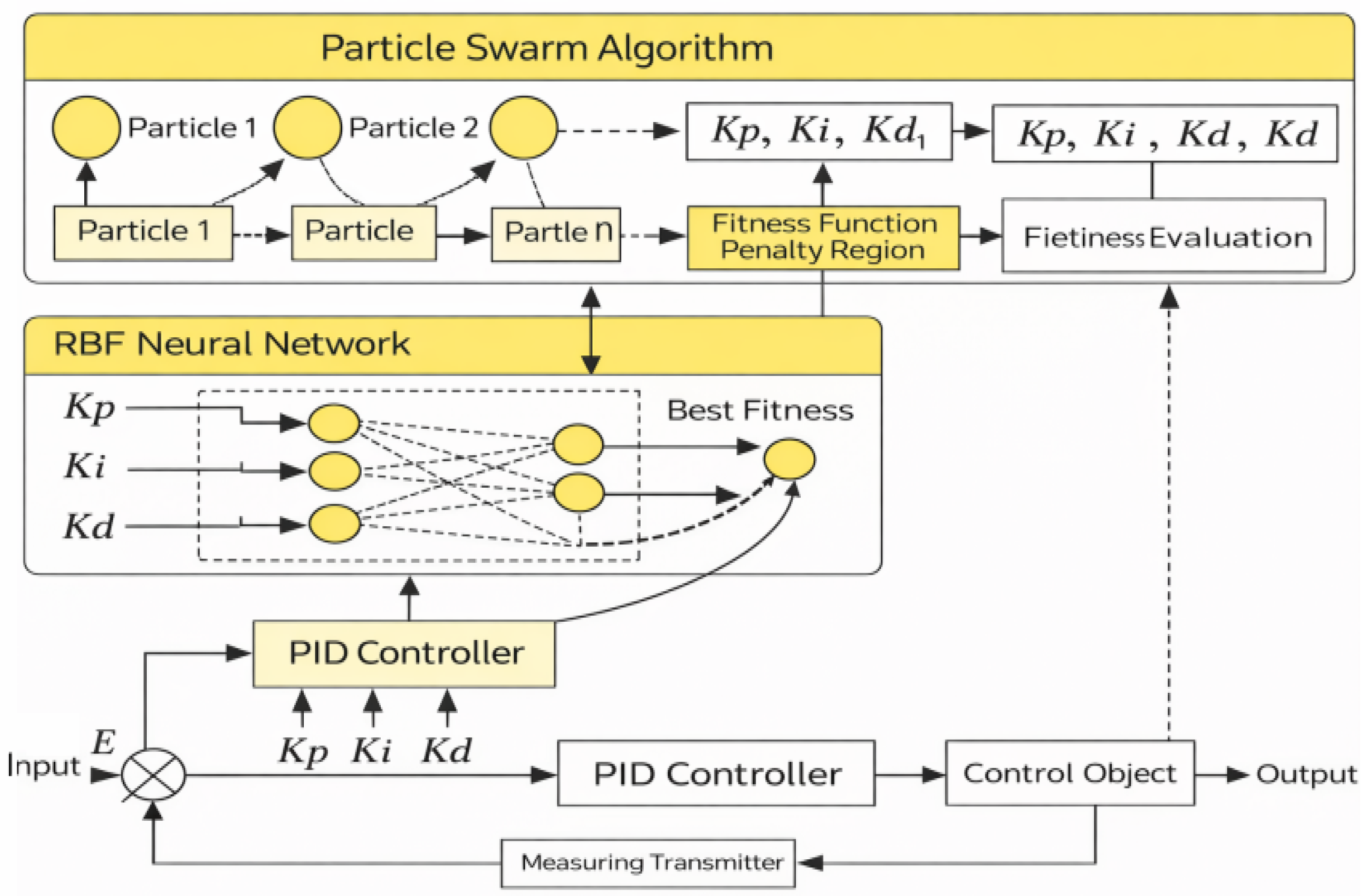
As the core framework of this study, the PSO–RBF–PID algorithm adopts a three-layer architecture integrating an RBF neural network, PSO-based optimization, and a PID closed-loop controller [26]. The RBF network approximates system dynamics, while PSO performs global optimization to tune network parameters and PID gains, enabling adaptive adjustment and improved handling of system nonlinearity and disturbances [27].

Specifically, the RBF neural network generates correction terms for PID parameters [28], and PSO iteratively updates particles based on $pBest$ and $gBest$ to obtain optimal parameters. These are applied to the PID controller to enhance control performance and robustness. The overall structure is shown in Figure 2.

Figure 2. Structure of the PSO-RBF-PID control system.

The RBF neural network adopts a three-layer structure consisting of an input layer, a hidden layer, and an output layer. The network is employed for both system identification and PID parameter approximation [29].

For system identification, the input vector is constructed as:

$$\begin{array}{c}{x}_1\left(t\right)=\left[u\right(t-1),u(t-2),y(t-1),y(t-2){]}^T\end{array}$$

(4)

The network output is the identified system output:

$$\begin{array}{c}\widehat{y}\left(t\right)={\displaystyle \sum _{i=1}^N}{w}_i^{\left(1\right)}\hspace{0.17em}{\varphi }_i\left(x_1\right(t\left)\right)\end{array}\hspace{0.17em}$$

(5)

For PID parameter approximation, the input vector is defined as:

$$\begin{array}{c}{x}_2\left(t\right)=\left[e\right(t),\dot{e}(t),\int e(t)\hspace{0.17em}dt{]}^T\end{array}$$

(6)

The network outputs the correction terms of PID parameters:

$$\begin{array}{c}{\left[\begin{array}{ccc}\mathsf{\Delta }{K}_p& \mathsf{\Delta }{K}_i& \mathsf{\Delta }{K}_d\end{array}\right]}^T={\displaystyle \sum _{i=1}^N}{w}_i^{\left(2\right)}\hspace{0.17em}{\varphi }_i\left(x_2\right(t\left)\right)\end{array}$$

(7)

The radial basis function adopts the Gaussian form:

$$\begin{array}{c}{\varphi }_i\left(x\right)=\mathit{exp}\left(-{\displaystyle \frac{\Vert x-c_i{\Vert }^2}{2{\sigma }_i^2}}\right)\end{array}$$

(8)

In this study, the number of hidden neurons was set to ($N$ = 10) based on preliminary simulation tests and a tradeoff between approximation accuracy and computational complexity. The hidden layer employs Gaussian radial basis functions, as defined in Equation (8). For system identification, the RBF network adopts a four-input, one-output structure. For PID parameter adaptation, the network uses a three-input, three-output structure, where the inputs are the tracking error, error derivative, and error integral, and the outputs correspond to the correction terms of ($K_p$), ($K_i$), and ($K_d$). The centers ($c_i$), widths (${\sigma }_i$), output weights ($w_i$), and initial PID gains are jointly optimized using the PSO procedure described in Section 3.2.

$N$ denotes the number of hidden-layer nodes, $c_i$ is the center vector, ${\sigma }_i$ is the width, and $w_i$ represents the output weight. In this study, the number of hidden nodes is set to $N=10$. The network parameters $c_i$, ${\sigma }_i$, and $w_i$ are optimized to achieve accurate nonlinear mapping and adaptive control. The complete PSO-RBF-PID optimization procedure is summarized in Algorithm 1.

Algorithm 1. PSO-RBF-PID optimization procedure for the 6-DOF underwater robot.

Input: Dynamic model, reference trajectory, disturbance model, sampling time Ts,    simulation time T, swarm size N, maximum iteration number Imax,    parameter bounds, and penalty coefficient λ. Output: Optimal parameter vector Θ *. 1: Initialize particle positions Θi and velocities Vi. 2: Decode each particle Θi into PID gains and RBF parameters. 3: Set the initial personal best Pi and global best G. 4: for k = 1 to Imax do 5:   for each particle i = 1, 2, …, N do 6:     Apply the decoded parameters to the PSO-RBF-PID controller. 7:     Run the closed-loop simulation under the predefined disturbance. 8:     Calculate tracking error e(t) and control input u(t). 9:     Evaluate the fitness value Ji. 10:      Update the personal best Pi if Ji is improved. 11:   end for 12:   Update the global best G. 13:   Update particle velocity and position. 14:   Apply boundary constraints. 15:   if the convergence criterion is satisfied then 16:     break 17:   end if 18: end for 19: Set Θ * = G. 20: Return Θ *.

In the present case study, the optimization was performed using the 6-DOF underwater robot model established in Section 2. The same step-response and helical trajectory-tracking tasks were used during controller evaluation. For each candidate particle, the closed-loop system was simulated under the predefined current disturbance and actuator constraints. The tracking error, settling behavior, and control effort were recorded to calculate the fitness value. After PSO convergence, the obtained optimal initial PID gains and RBF parameters were fixed as the final controller parameters. The final controller was then tested under the same benchmark conditions as PID, cascade PID, fuzzy PID, FOPID, and PSO-PID.

Particle swarm optimization (PSO) is employed to optimize both the PID controller parameters and the RBF neural network parameters due to its strong global search capability and simple implementation [30,31].

For joint optimization, each particle is defined as:

$$\begin{array}{c}{x}_i=\left[K_p,K_i,K_d,c,\sigma ,w\right]\end{array}$$

(9)

To satisfy multi-parameter collaborative optimization, a real-valued encoding strategy is adopted. Each particle is represented as a 33-dimensional vector [20,21]:

$$\begin{array}{c}{X}_i=[c_1,\dots ,c_{10},{\sigma }_1,\dots ,{\sigma }_{10},w_1,\dots ,w_{10},K_p^0,K_i^0,K_d^0]\end{array}$$

(10)

where the first 30 dimensions correspond to the RBF parameters, and the last three represent the initial PID parameters.

The fitness function is defined based on the ITAE (time-weighted absolute error) criterion with a control penalty term [32]:

$$\begin{array}{c}J={\int }_0^{T}t\hspace{0.17em}\left|e\right(t\left)\right|\hspace{0.17em}dt+\lambda {\int }_0^T|u\left(t\right)|\hspace{0.17em}dt\end{array}$$

(11)

where T is the simulation time, $e\left(t\right)$ is the tracking error, $u\left(t\right)$ is the control input, and $\lambda$ is the penalty coefficient (set to 0.01).

The particle velocity and position are updated according to [27]:

$$\begin{array}{c}{v}_{id}(k+1)=\omega v_{id}\left(k\right)+c_1{r}_1(pBes{t}_{id}-x_{id}(k\left)\right)+c_2{r}_2(gBes{t}_d-x_{id}(k\left)\right)\end{array}$$

(12)

$$\begin{array}{c}{x}_{id}(k+1)=x_{id}\left(k\right)+v_{id}(k+1)\end{array}$$

(13)

where $\mathrm{d}=1,2,\dots ,33$, $\mathsf{\omega }=0.7$ is the inertia weight, $c_1=c_2=1.49$ are acceleration coefficients, and $r_1,r_2\in [0,1]$ are random variables.

Through iterative updates, the optimal parameters are obtained, enabling coordinated optimization of both RBF and PID parameters while reducing the risk of convergence to local optima.

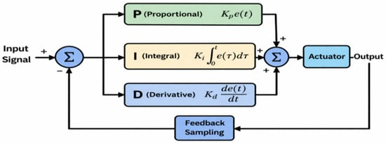
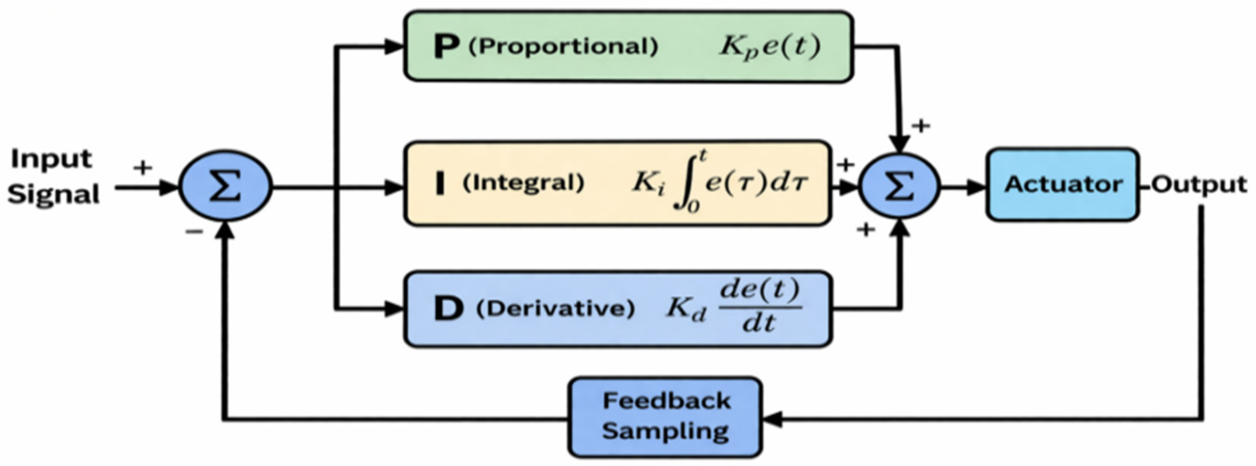
This module forms the core of the control system, where PID parameters are adaptively updated by the RBF network, and the resulting control input is allocated to thrusters, with system output fed back to achieve closed-loop control. For comparison, the structure of the traditional PID closed-loop control system is illustrated in Figure 3.

Figure 3. Traditional PID control system.

3.2. Optimization Process

The optimization procedure consists of the following steps:

• Initialization: Set swarm size N = 20, maximum iterations Tmax = 40, and initialize particles within predefined bounds.
• Simulation: Map particle parameters to the PSO-RBF-PID controller and perform system simulation.
• Evaluation: Compute the fitness value using the defined objective function.
• Update: Update personal best (pBest) and global best (gBest).
• Iteration: Update particle velocity and position with boundary constraints.
• Termination: Output the optimal parameters when convergence criteria or maximum iterations are satisfied.

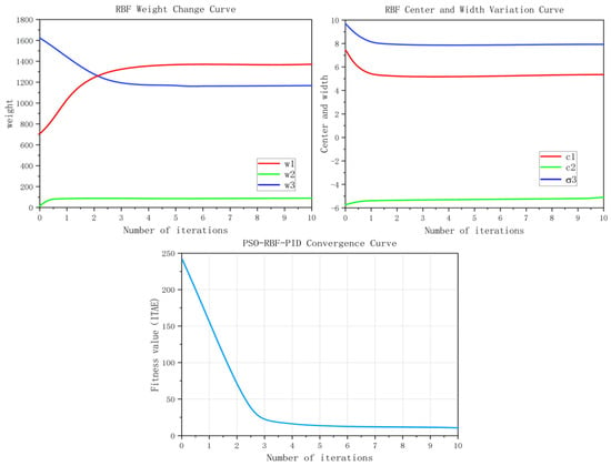
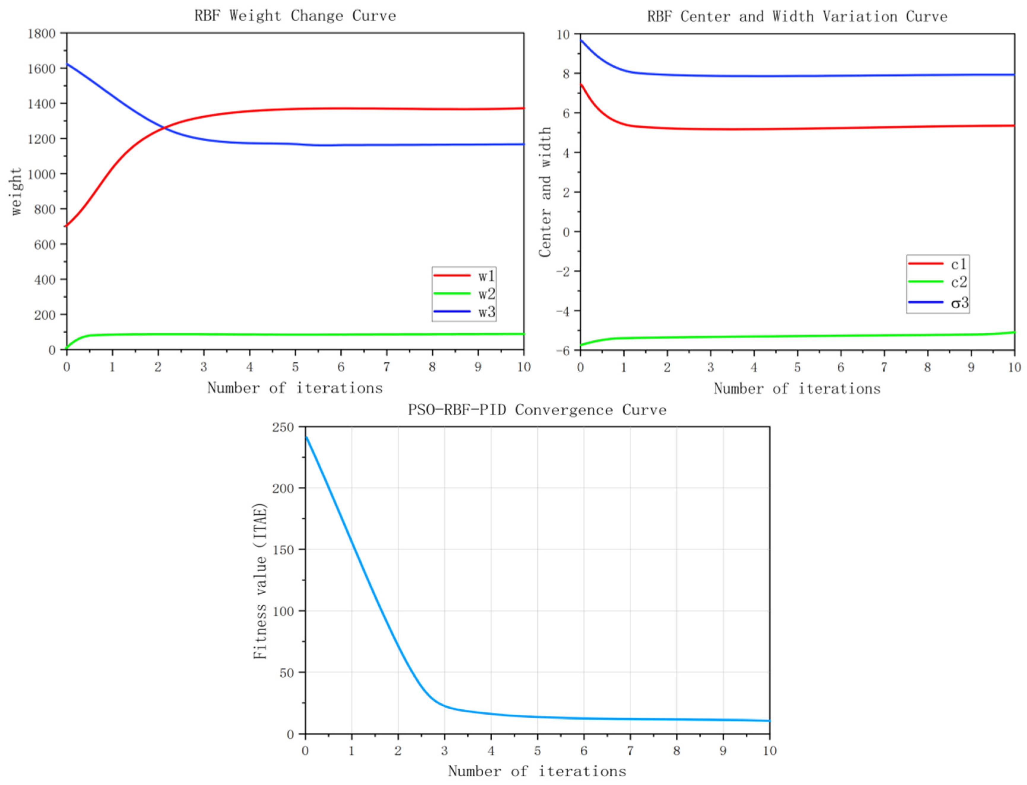
The PSO parameters were determined through repeated simulations and preliminary sensitivity analysis. Considering optimization performance and computational cost, (N = 20), (Tmax = 40), (w = 0.7), and ($c_1=c_2=1.49$) were selected. As shown in the fitness convergence curve in the first sub-figure of the parameter trend chart in Section 4.2.5, the global best fitness value decreases rapidly and gradually converges, indicating stable optimization performance under the chosen parameter settings.

The optimized parameters are subsequently used for real-time adaptive PID tuning via the RBF neural network.

3.3. Stability and Performance Analysis

To rigorously analyze the stability and convergence of the proposed PSO-RBF-PID control method, the nonlinear dynamics of the underwater robotic system are described as:

$$\begin{array}{c}\dot{x}\left(t\right)=f(x,t)+b\hspace{0.17em}u\left(t\right)\end{array} y\left(t\right)=x\left(t\right)$$

(14)

where $f(x,t)$ represents the nonlinear system dynamics, and $b$ is a positive constant.

The tracking error is defined as:

$$e\left(t\right)=r\left(t\right)-y\left(t\right)$$

(15)

The proposed controller can be expressed as:

$$\begin{array}{c}u\left(t\right)=K_p\left(t\right)e\left(t\right)+K_i\left(t\right){\int }_0^{t}e\left(\tau \right)\hspace{0.17em}d\tau +K_d\left(t\right)\dot{e}\left(t\right)\end{array}$$

(16)

The adaptive parameters are generated by the RBF neural network:

$$\begin{array}{c}{K}_p\left(t\right)=W_p^T\Phi \left(x\right),\hspace{1em}{K}_i\left(t\right)=W_i^T\Phi \left(x\right),\hspace{1em}{K}_d\left(t\right)=W_d^T\Phi \left(x\right)\end{array}$$

(17)

where $\Phi \left(x\right)$ is the radial basis function vector, and $W_p,W_i,W_d$ are the corresponding weight vectors optimized by the PSO algorithm.

To analyze system stability, a Lyapunov candidate function is selected as:

$$\begin{array}{c}V\left(t\right)={\displaystyle \frac{1}{2}}{e}^2\left(t\right)\end{array}$$

(18)

Taking the time derivative yields:

$$\begin{array}{c}\dot{V}\left(t\right)=e\left(t\right)\dot{e}\left(t\right)\end{array}$$

(19)

The error dynamics can be written as:

$$\begin{array}{c}\dot{e}\left(t\right)=\dot{r}\left(t\right)-\dot{y}\left(t\right)=\dot{r}\left(t\right)-f(x,t)-b\hspace{0.17em}u\left(t\right)\end{array}$$

(20)

Substituting the control law into the error dynamics gives:

$$\begin{array}{c}\dot{e}\left(t\right)=\dot{r}\left(t\right)-f(x,t)-b\left[K_p\left(t\right)e\left(t\right)+K_i\left(t\right){\int }_0^{t}e\left(\tau \right)\hspace{0.17em}d\tau +K_d\left(t\right)\dot{e}\left(t\right)\right]\end{array}$$

(21)

Rearranging yields:

$$\begin{array}{c}(1+b{K}_d(t\left)\right)\dot{e}\left(t\right)=\dot{r}\left(t\right)-f(x,t)-b{K}_p\left(t\right)e\left(t\right)-b{K}_i\left(t\right){\int }_0^{t}e\left(\tau \right)\hspace{0.17em}d\tau \end{array}$$

(22)

By properly designing the adaptive parameters $K_p\left(t\right),K_i\left(t\right)\mathrm{and}{K}_d\left(t\right)$, it can be ensured that:

$$\begin{array}{c}\dot{V}\left(t\right)\le -c{e}^2\left(t\right),\hspace{1em}c>0\end{array}$$

(23)

Therefore, the closed-loop system is stable in the sense of Lyapunov.

Furthermore, since $\dot{V}\left(t\right)\le -c{e}^2\left(t\right)$, it follows that:

$$\begin{array}{c}e\left(t\right)\in L_2\cap L_{\infty }\end{array}$$

(24)

By Barbalat’s lemma, one obtains:

$$\begin{array}{c}\underset{t\to \infty }{\mathit{lim}}e\left(t\right)=0\end{array}$$

(25)

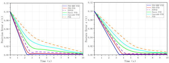
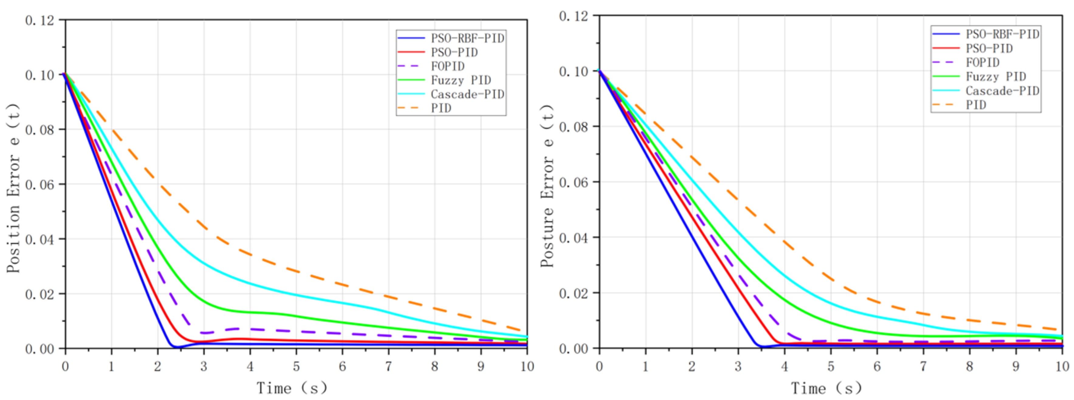
The position and attitude error convergence characteristics of the six controllers are shown in Figure 4:

Figure 4. Six control algorithm position and posture errors.

This proves the asymptotic convergence of the tracking error.

In addition, the boundedness of the control input is analyzed. The control signal satisfies:

$$\begin{array}{c}\left|u\right(t\left)\right|\le K_p\left|e\right(t\left)\right|+K_i{\int }_0^t|e\left(\tau \right)|\hspace{0.17em}d\tau +K_d|\dot{e}\left(t\right)|\end{array}$$

(26)

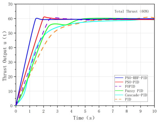
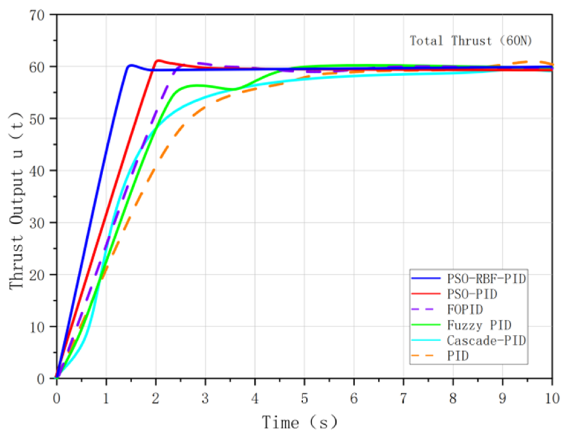
The boundedness of the tracking error, its derivative, and adaptive parameters ensures that the control input $u\left(t\right)$ remains bounded. As shown in the following figure, the control input (thrust output) for various controllers demonstrates the system’s stable response over time, with all controllers maintaining bounded thrust output within the expected limits.

As shown in Figure 5, compared with other algorithms, the proposed PSO-RBF-PID method can produce outputs with smaller fluctuations, faster convergence, and smoother control signals.

Figure 5. Thruster output response.

3.4. Sensitivity Analysis

To assess the robustness of the selected PID parameters, a sensitivity analysis was conducted by introducing small variations to the PID parameters $Kp$, $Ki$ and $Kd$. The performance was evaluated by computing the partial derivatives of the system output $y\left(t\right)$ with respect to each parameter:

$$S_{K_p}={\displaystyle \frac{\mathsf{\partial }y\left(t\right)}{\mathsf{\partial }{K}_p}},\hspace{1em}{S}_{K_i}={\displaystyle \frac{\mathsf{\partial }y\left(t\right)}{\mathsf{\partial }{K}_i}},\hspace{1em}{S}_{K_d}={\displaystyle \frac{\mathsf{\partial }y\left(t\right)}{\mathsf{\partial }{K}_d}}$$

(27)

The sensitivity index $\mathsf{\Delta }\mathrm{E}$ was calculated as the relative change in performance:

$$\mathsf{\Delta }E={\displaystyle \frac{E_{new}-E_{base}}{E_{base}}}$$

(28)

The results showed that steady-state error changes were less than 0.1%, and no significant impact was observed on regulation time or overshoot, confirming the robustness of the PID parameters. The sensitivity analysis validates that the selected PID parameters provide stable, reliable performance even under perturbations, ensuring their suitability for high-precision control tasks. All subsequent parameter selections were also validated through a similar sensitivity analysis.

3.5. Highlights of PSO-RBF-PID Algorithm

Compared with traditional PID, Cascade PID, fuzzy PID, FOPID and PSO-PID methods, the proposed PSO-RBF-PID approach has two main advantages. First, it optimizes not only the initial PID gains but also the RBF network parameters, including centers, widths, and weights, which improves the nonlinear approximation capability of the controller. Second, unlike purely offline metaheuristic optimization methods such as GA-based parameter search, the proposed method retains an online adaptive mechanism through the RBF network. This enables the controller to compensate for model uncertainty and environmental disturbances during operation. Therefore, the proposed method is particularly suitable for high-precision trajectory tracking and disturbance rejection in the considered 6-DOF multi-thruster underwater robot [33].

4. Simulation Experiments and Comparative Analysis

4.1. Simulation Experimental Design

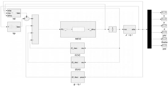
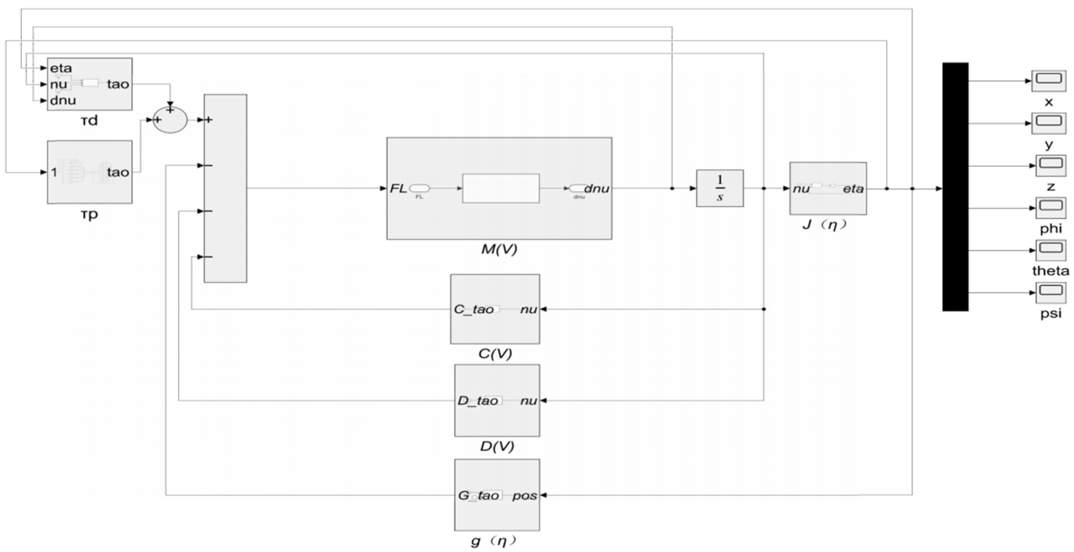
To evaluate the proposed PSO-RBF-PID controller, a MATLAB (R2024a)/Simulink-based simulation case study was developed for the 6-DOF multi-thruster underwater robot with hydrodynamic disturbances, as shown in Figure 6. No real underwater robot experiment or water-tank test was conducted in this work. All controllers were implemented under the same dynamic model, reference inputs, disturbance conditions, actuator constraints, and evaluation indices. In the simulation framework, each controller is integrated into the thrust control module ($\tau$) and coupled with the robot motion states through feedback loops, ensuring a consistent comparison among different control strategies.

Figure 6. Dynamics model of underwater robot.

The six controllers, namely PID, cascade PID, fuzzy PID, FOPID, PSO-PID, and PSO-RBF-PID, are implemented in Simulink R2024a using the same underwater robot dynamic model. The simulation results are evaluated using steady-state error, settling time, overshoot, and integral absolute error [34]. Therefore, the results should be interpreted as comparative simulation evidence for the considered 6-DOF underwater robot case study, rather than as direct experimental validation on a physical underwater robot.

Two main experiments are performed: a step response test to evaluate dynamic response and steady-state accuracy and a spiral trajectory tracking test to assess multi-degree-of-freedom tracking performance. In addition, an ocean current disturbance scenario is introduced to examine disturbance rejection capability.

A unified evaluation framework is adopted with four performance indices: steady-state error (SSE), regulation time (${\mathrm{T}}_{\mathrm{s}}$), overshoot, and integral of absolute error (IAE), where smaller values indicate better performance.

All six controllers were evaluated under the same model, sampling period, simulation time, reference inputs, thrust limits, disturbances, and performance indices. The simulation parameters are set as follows: sampling period of 0.1 s and total simulation time of 100 s. The step input amplitude is 0.1 (0.1 m for position and 0.1 rad for attitude). The spiral trajectory consists of sinusoidal motion along the x-axis, cosine motion along the y-axis, and linear descent along the z-axis. The external disturbance is modeled as a combination of steady and time-varying ocean currents. In addition to a constant current (0.2 m/s at 45°), time-varying components such as sinusoidal fluctuations are introduced to partially reflect the variability of real underwater environments.

To enhance the practical relevance of the simulations, additional non-ideal factors commonly encountered in real underwater robotic systems are considered. These include:

• Parametric uncertainty: Key hydrodynamic coefficients are perturbed to simulate modeling errors;
• External disturbances: Time-varying and composite disturbances are introduced, including sinusoidal and step components;
• Actuator constraints: Saturation limits are imposed on thruster outputs to reflect physical limitations;
• Sensor imperfections: Measurement noise and time delay are introduced to emulate realistic sensing conditions.

These settings aim to approximate real-world uncertainties and provide a more rigorous evaluation of controller robustness.

4.2. Simulation Experiments

4.2.1. Simulation of Traditional PID

The PID parameters for each degree of freedom were determined through repeated simulations under the unified benchmark conditions in Section 4.1 and further refined by sensitivity analysis. The final gains were selected based on comprehensive performance indices to ensure the consistency, reliability, and robustness of the controller settings. Accordingly, six independent PID controllers were designed for the underwater robot [22,35]. The traditional PID control system design is shown in Figure 7.

Figure 7. Traditional PID control system design.

Parameter Setting:

The PID parameters for each degree of freedom were determined through multiple independent simulation trials. Specifically, the experiments were conducted under the unified reference conditions outlined in Section 4.1, with repeated tests and sensitivity analysis to ensure robustness. For each degree of freedom, the system optimizes the PID gain parameters by evaluating control performance across several iterations, selecting the final parameter set based on a comprehensive performance index. This approach ensures the consistency and reliability of the parameter settings. Independent PID controllers were designed for each of the six degrees of freedom of the underwater robot.

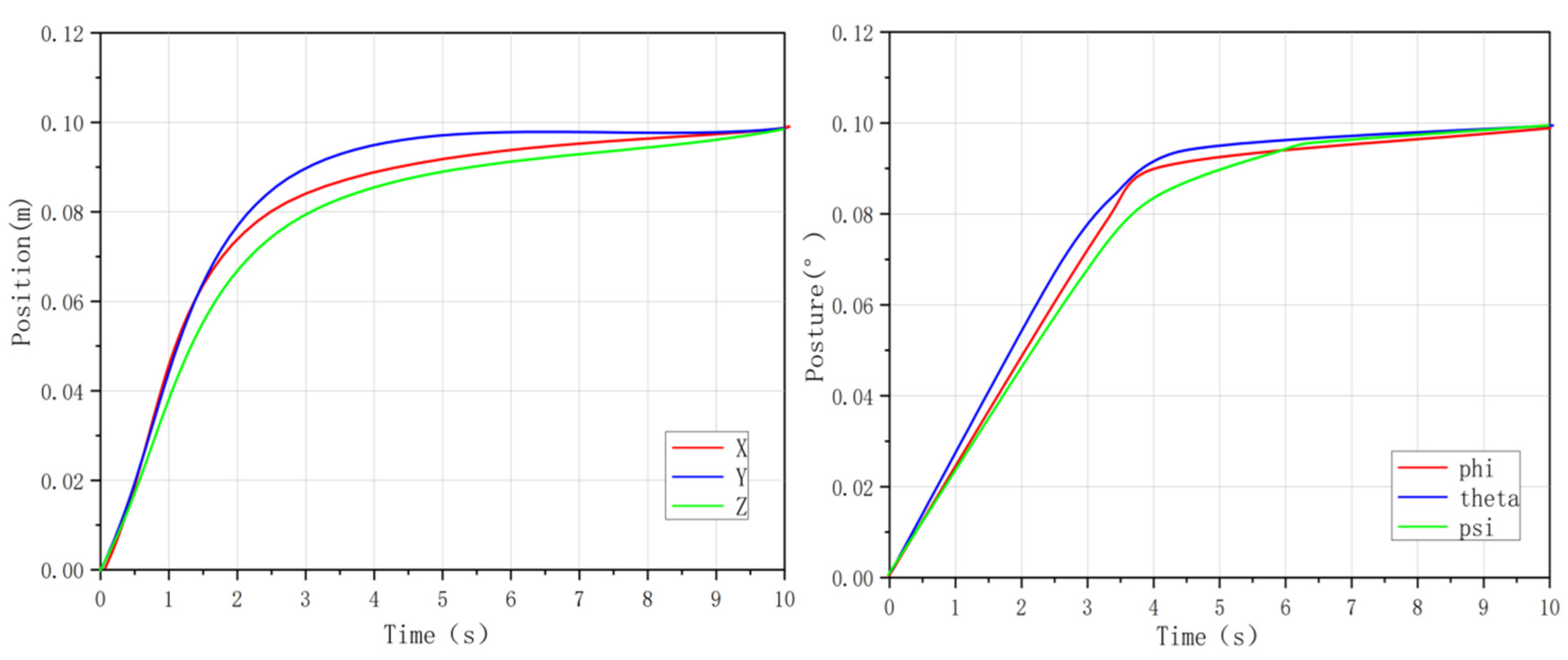
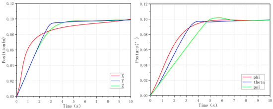
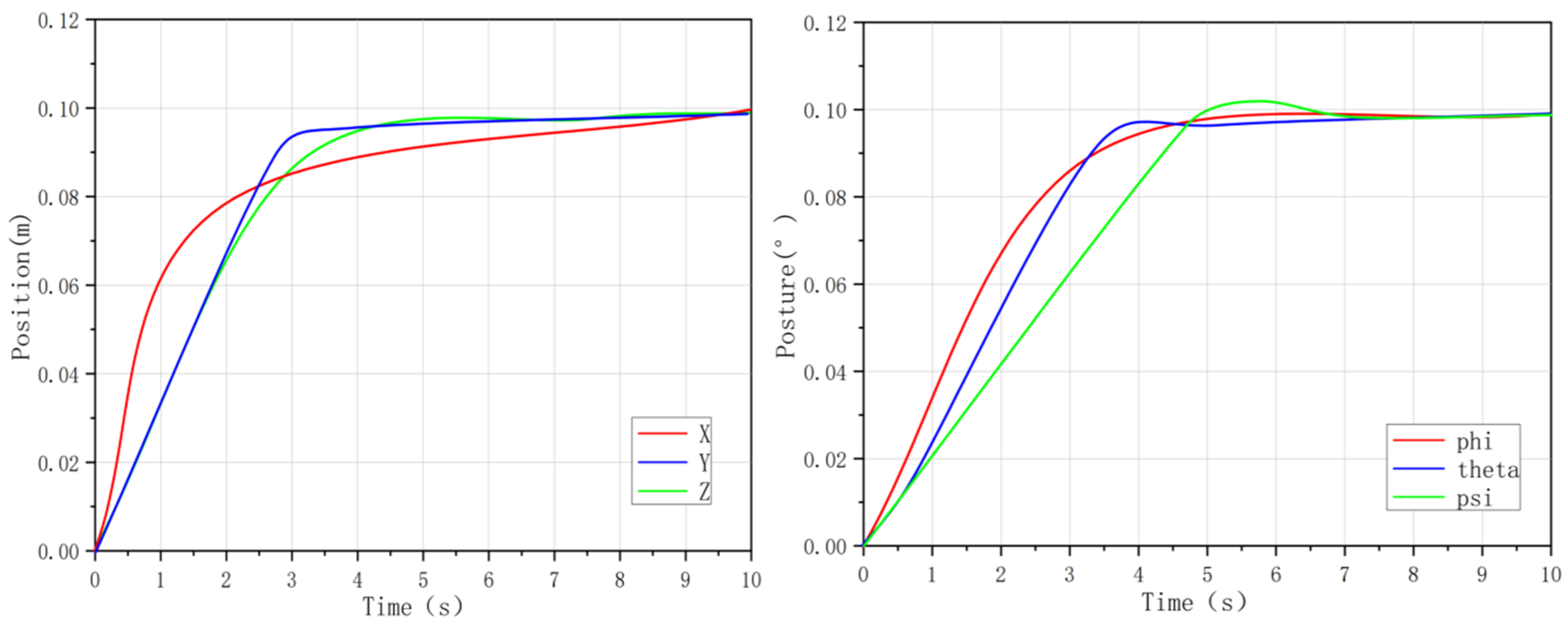
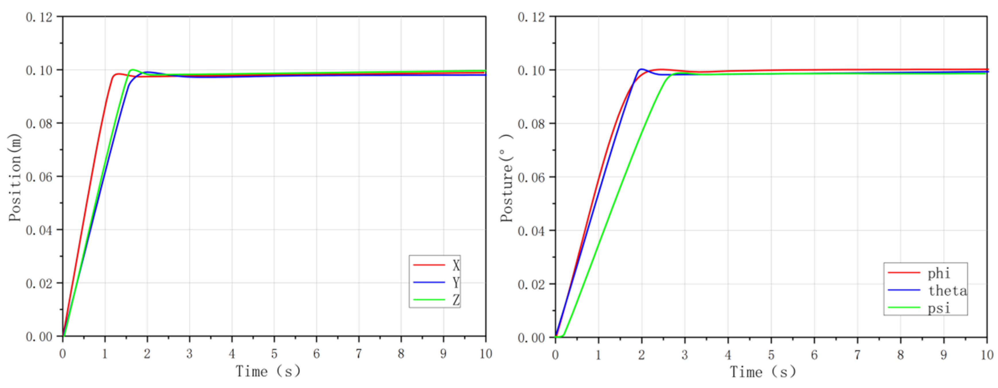
The step response curves of the traditional PID controller are shown in Figure 8:

Figure 8. Traditional PID step response curve.

The spiral trajectory response curve of the traditional PID controller is shown in Figure 9:

Figure 9. Traditional PID spiral trajectory response curve.

Experimental Results and Analysis:

The simulation results indicate that while traditional PID can provide basic stable control for the 6-degree-of-freedom underwater robot, it exhibits significant shortcomings in dynamic response and steady-state accuracy. In the step response test, the steady-state errors of the x, y, z, and roll ($\varphi$) channels are 0.014178, 0.014246, 0.015165, and 0.015156 m/rad, respectively, with regulation times of about 10 s, while the overshoot of the pitch ($\theta$) and yaw ($\psi$) channels reaches 1.192198%. In the spiral trajectory tracking task, the x-axis steady-state error is 0.1861 m, the overshoot is 12.5%, and the IAE index is 145.95. These results indicate that the fixed-parameter structure limits the overall control performance, making it difficult to effectively compensate for system nonlinearity and coupling effects and therefore cannot fully satisfy the requirements of high-precision underwater operations in terms of control accuracy and response speed. The detailed performance figures of the traditional PID are shown in Table 2 and Table 3.

Table 2. Traditional PID step response performance.

Algorithm	Degree of Freedom	SSE	Ts/s	OS/%	IAE
Traditional PID	x	0.014178	10	0.102331	0.56878
	y	0.014246	10	0.101459	0.57897
	z	0.015165	10	0.100215	0.55916
	phi	0.015156	10	0.113216	0.56514
	theta	0.002789	9.38	1.192198	0.40318
	psi	0.002756	9.41	1.192198	0.40645

Table 3. Traditional PID spiral trajectory response performance.

Algorithm	Degree of Freedom	SSE	Ts/s	OS/%	IAE	ITAE
Traditional PID	x	0.1861	18.4	12.5	145.95	7291.0
	y	0.1658	16.9	10.7	134.65	6638.5
	z	0.4468	12.6	6.0	286.54	14,274.0
	phi	0.0033	5.4	8.6	1.47	76.4
	theta	0.0038	6.4	15.4	1.71	86.0
	psi	0.0037	5.8	11.8	1.54	78.0

4.2.2. Design of Cascade PID

To further evaluate the effectiveness of the proposed control strategy, a cascade PID controller is introduced for comparison. The cascade structure consists of an outer position loop and an inner velocity loop. The outer loop tracks the reference position and generates the desired velocity, while the inner loop regulates actuator dynamics to ensure fast response and disturbance rejection.

The control laws are given by:

$$u_1\left(t\right)=K_{p1}{e}_1\left(t\right)+K_{i1}\int e_1\left(t\right)\hspace{0.17em}dt+K_{d1}{\displaystyle \frac{d{e}_1\left(t\right)}{dt}}$$

(29)

$$u\left(t\right)=K_{p2}{e}_2\left(t\right)+K_{i2}\int e_2\left(t\right)\hspace{0.17em}dt+K_{d2}{\displaystyle \frac{d{e}_2\left(t\right)}{dt}}$$

(30)

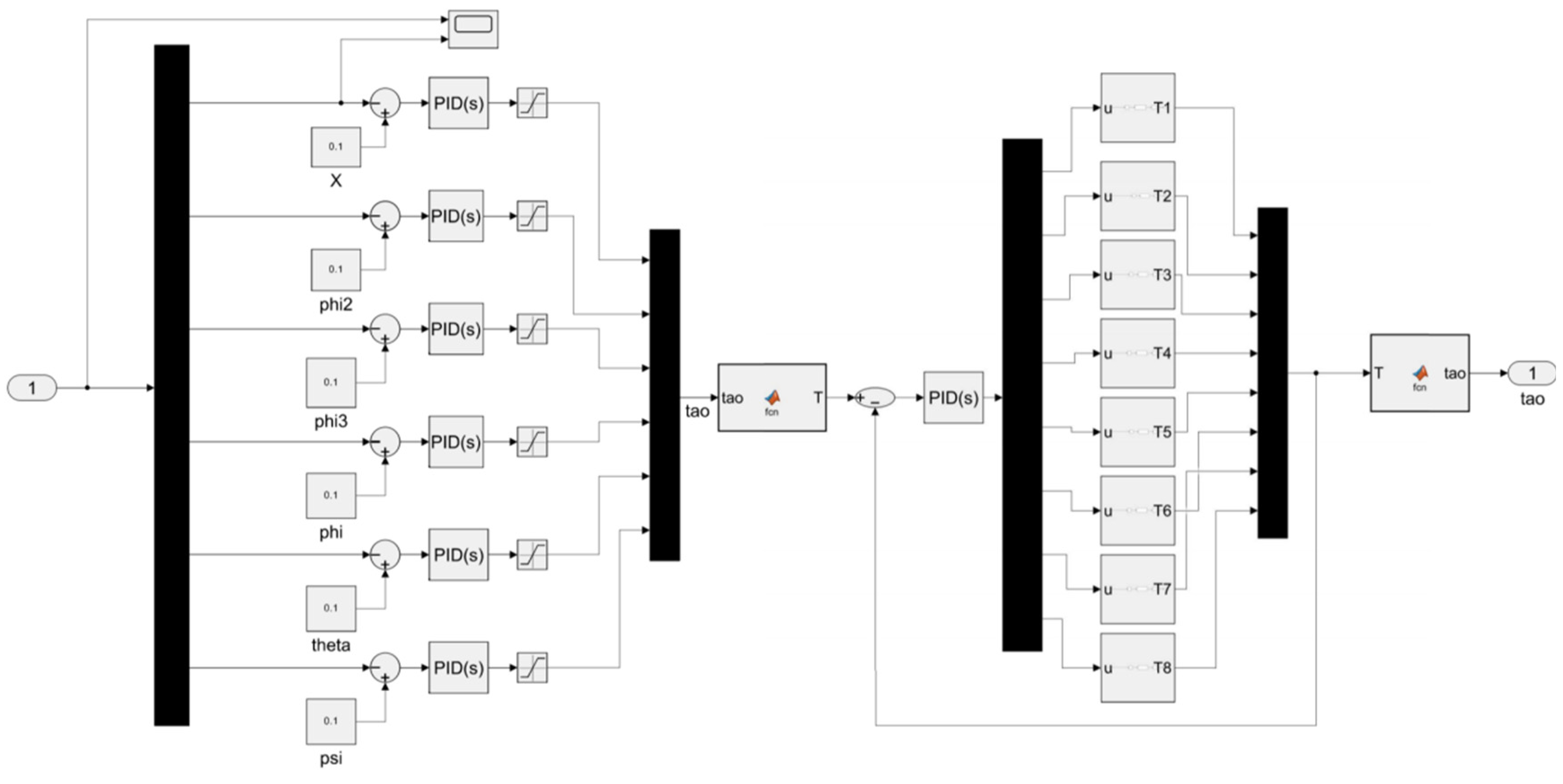
The Simulink implementation of the cascade PID controller module is shown in Figure 10:

Figure 10. Design of Cascade PID Controller Module.

The Simulink diagrams, such as the cascade PID controller module, are provided to illustrate the benchmark controller implementation and improve simulation reproducibility. The cascade PID controller was constructed in Simulink as one of the comparative algorithms. These diagrams show the connection of feedback signals and controller modules in the simulation environment, rather than hardware implementation or experimental platform schematics. Therefore, only representative diagrams are retained in the main text. The step response curves of the cascade PID controller are shown in Figure 11.

Figure 11. Cascade PID step response curve.

$u_1\left(t\right)$ is the output of the outer loop (desired velocity), $u\left(t\right)$ is the final control input, and $e_1\left(t\right)$, $e_2\left(t\right)$ denote position and velocity errors, respectively.

The cascade PID controller is implemented in Simulink and applied to the thrust control loop of the underwater robot. The outer loop generates the velocity reference, while the inner loop produces the control input to regulate the propulsion system. Controller parameters are tuned empirically to ensure stability and a fair comparison. As a representative engineering control scheme, the cascade PID provides a benchmark for evaluating the proposed PSO-RBF-PID method. The detailed performance figures of the cascade PID are shown in Table 4 and Table 5.

Table 4. Cascade PID step response performance.

Algorithm	Degree of Freedom	SSE	Ts/s	OS/%	IAE
Cascade PID	x	0.013478	10	0.102296	0.53722
	y	0.013778	10	0.101451	0.54896
	z	0.013997	10	0.100209	0.51437
	phi	0.013466	9.78	2.253731	0.54435
	theta	0.002687	8.93	2.364492	0.47652
	psi	0.002683	8.94	2.459642	0.49635

Table 5. Cascade PID spiral trajectory response performance.

Algorithm	Degree of Freedom	SSE	Ts/s	OS/%	IAE	ITAE
Cascade PID	x	0.1813	18.2	12.2	144.31	7188.1
	y	0.1656	16.6	9.8	131.78	6448.3
	z	0.4415	12.2	5.8	281.73	14,237.0
	phi	0.0028	5.3	8.4	1.45	72.5
	theta	0.0038	6.3	15.1	1.63	77.0
	psi	0.0036	5.6	11.6	1.51	75.0

4.2.3. Fuzzy PID Control Simulation Analysis

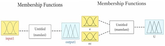
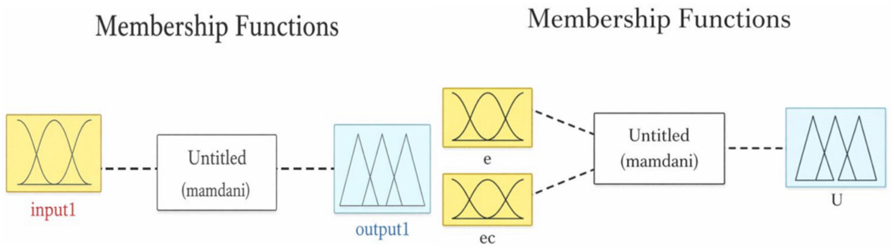
Fuzzy PID is a hybrid control strategy combining traditional PID and fuzzy logic. It uses real-time error $e$ and error change rate $e_c$ as inputs, applies fuzzy rules based on expert experience, and dynamically adjusts PID parameters for online adaptation. While it offers better adaptability to dynamic system changes compared to traditional PID, its performance is limited by the completeness and subjectivity of the fuzzy rule base, making optimal control difficult in strong coupling and large disturbance scenarios [20,29,35]. The designed fuzzy control membership functions are shown in Figure 12.

Figure 12. Design of fuzzy control membership function.

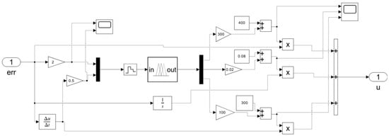
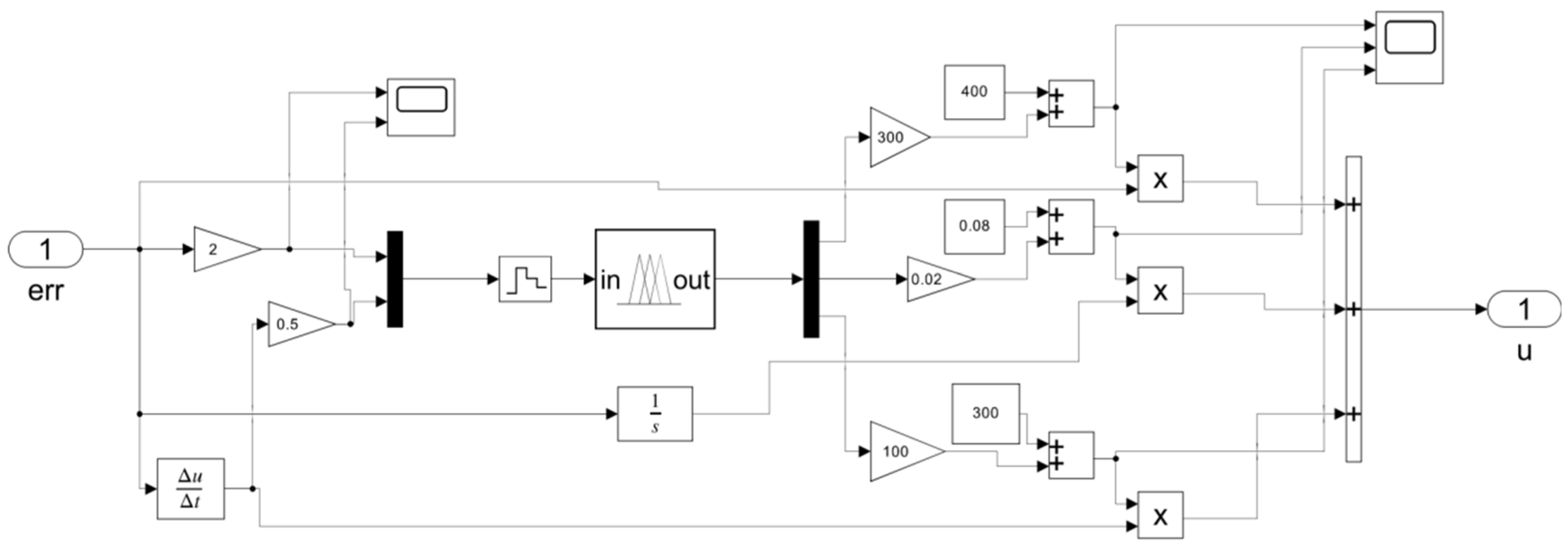
The fuzzy controller module implemented in Simulink is shown in Figure 13:

Figure 13. Design of fuzzy controller module.

Parameter Setting:

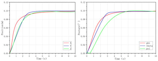
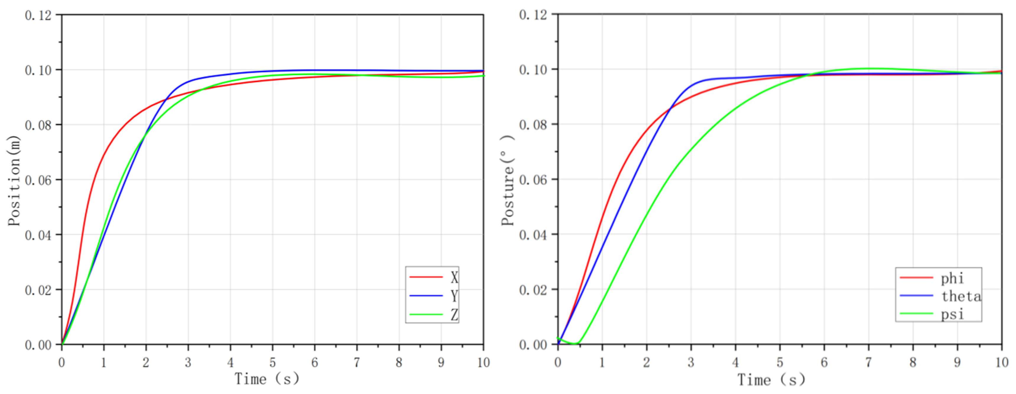
Independent fuzzy PID controllers are designed for each degree of freedom, with tracking error as the input. All controller parameters—including the fuzzy rule base, scaling factors, and input–output domains—are determined through sensitivity analysis and repeated simulations, rather than manual tuning. Specifically, small perturbations are applied to each parameter, and the resulting variations in performance indices are assessed to select parameter sets with low sensitivity, ensuring robustness and reproducibility. A Mamdani-type inference mechanism with centroid defuzzification is used, and the universes of discourse are iteratively refined based on system dynamics to enhance control performance. The step response curves of the fuzzy PID controller are shown in Figure 14.

Figure 14. Fuzzy PID step response curve.

Experimental Results and Analysis:

The simulation results show that the control performance of fuzzy PID is significantly improved compared to traditional PID. In the step response test, the six−channel steady-state error drops to 0.003065−0.003478 m/rad, about 78% lower than that of traditional PID. The regulation time for the pitch and yaw channels is shortened to 7.58 s with an overshoot of 2.624653%. The IAE index is 15−20% lower than that of traditional PID. In the spiral trajectory tracking task, the x−axis steady-state error is 0.1741 m, the overshoot is 11.4%, and the IAE index is 142.21. However, due to the subjectivity of the fuzzy rule base, the algorithm shows a slight increase in overshoot, insufficient dynamic tracking speed in multi-degree−of−freedom coupling scenarios, and limited ability to suppress random disturbances. The detailed performance figures of the fuzzy PID are shown in Table 6 and Table 7.

Table 6. Fuzzy PID step response performance.

Algorithm	Degree of Freedom	SSE	Ts/s	OS/%	IAE
Fuzzy PID	x	0.003065	10	0.101364	0.48314
	y	0.003478	10	0.101332	0.45723
	z	0.003388	10	0.101043	0.47305
	phi	0.003497	9.71	0.101545	0.48316
	theta	0.002721	7.58	2.624653	0.31898
	psi	0.002638	7.51	2.624784	0.31917

Table 7. Fuzzy PID spiral trajectory response performance.

Algorithm	Degree of Freedom	SSE	Ts/s	OS/%	IAE	ITAE
Fuzzy PID	x	0.1741	18.1	11.4	142.21	7143.0
	y	0.1437	15.8	8.7	128.67	5897.7
	z	0.4396	11.8	5.5	283.68	14,354.0
	phi	0.0028	5.2	8.5	1.45	72.4
	theta	0.0036	6.1	14.9	1.52	69.0
	psi	0.0033	5.5	11.4	1.47	73.0

4.2.4. Simulation Analysis of FOPID Control

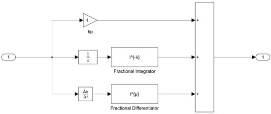
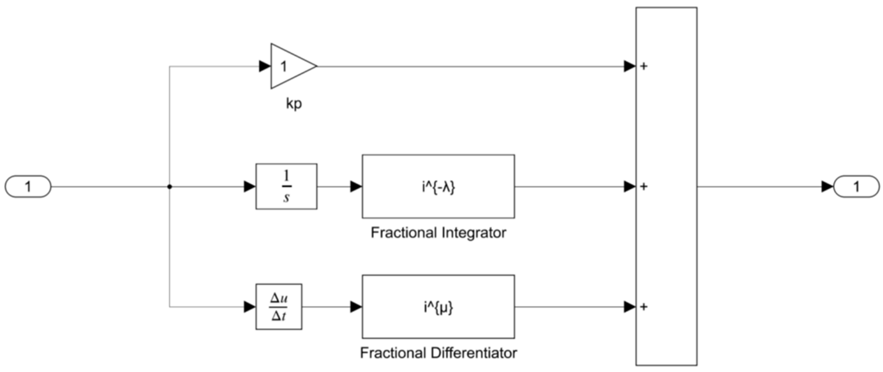
To further evaluate the effectiveness of the proposed method, a fractional-order PID (FOPID) controller is introduced for comparison. Compared with the conventional PID controller, FOPID incorporates fractional-order integration and differentiation, offering additional tuning flexibility and improved dynamic performance. The FOPID controller design is shown in Figure 15.

Figure 15. Design of FOPID controller.

The control law is expressed as:

$$u\left(t\right)=K_{p}e\left(t\right)+K_i{D}^{-\lambda }e\left(t\right)+K_d{D}^{\mu }e\left(t\right)$$

(31)

$$G\left(s\right)=K_p+{\displaystyle \frac{K_i}{s^{\lambda }}}+K_d{s}^{\mu }$$

(32)

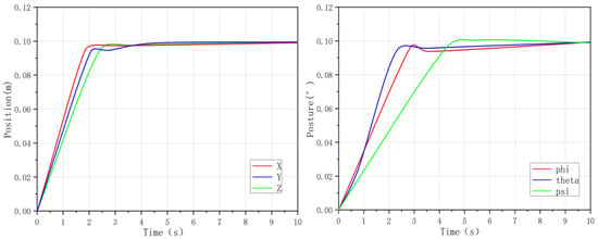
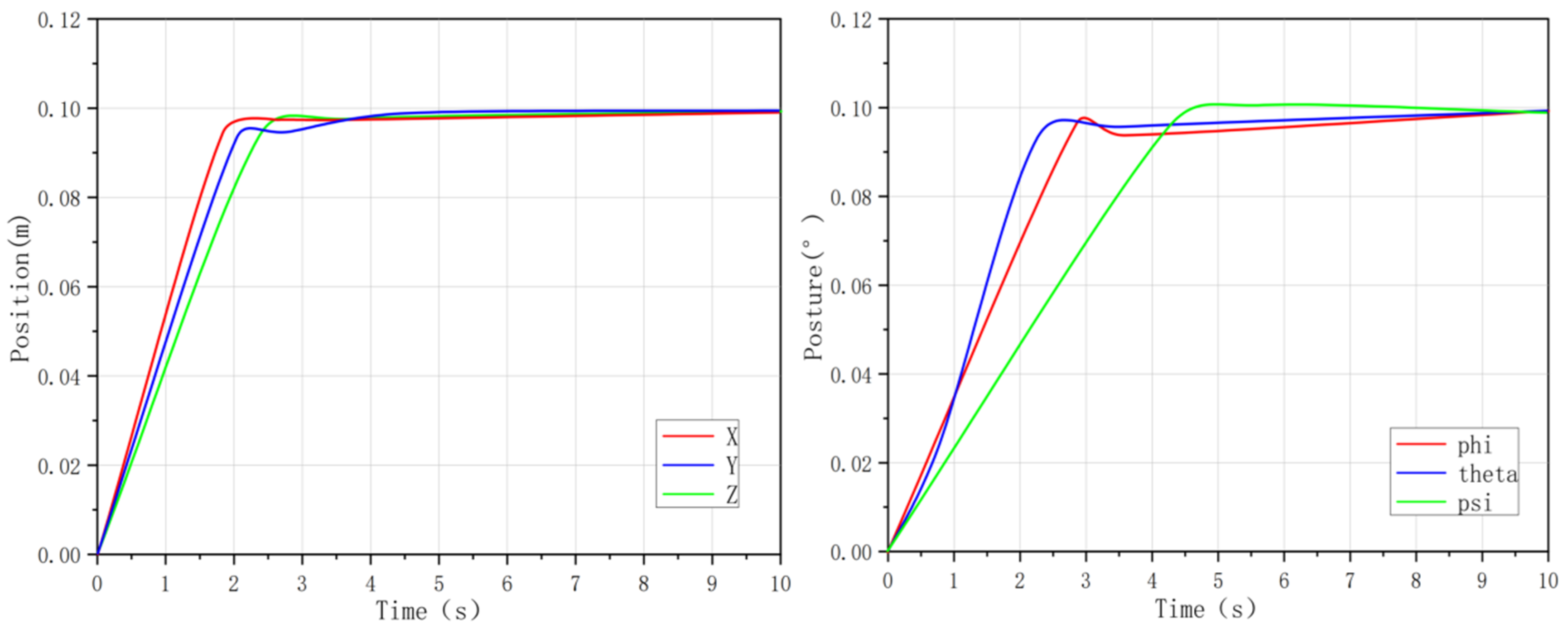
The step response curves of the FOPID controller are shown in Figure 16:

Figure 16. FOPID step response curve.

$K_p,K_i$ and $K_d$ are the proportional, integral, and derivative gains, and $\lambda ,\mu$ (with 0 < $\lambda$, $\mu$ ≤ 1) represent the fractional orders. The FOPID controller, implemented in Simulink using the Oustaloup recursive approximation, regulates the propulsion system of the underwater robot based on tracking errors.

FOPID parameters ($K_p,K_i,K_d,\lambda ,\mu$) are optimized through iterative simulations and sensitivity analysis, ensuring optimal control performance. This method provides a benchmark for evaluating the PSO-RBF-PID algorithm. The detailed performance numbers of the FOPID are shown in Table 8 and Table 9.

Table 8. FOPID step response performance.

Algorithm	Degree of Freedom	SSE	Ts/s	OS/%	IAE
FOPID	x	0.000412	9.18	0.443781	0.42856
	y	0.000513	9.45	0.538244	0.42238
	z	0.000478	9.42	0.563215	0.44356
	phi	0.000698	9.25	1.376574	0.37482
	theta	0.001238	7.04	1.496884	0.30113
	psi	0.001307	7.16	1.525748	0.30337

Table 9. FOPID spiral trajectory response performance.

Algorithm	Degree of Freedom	SSE	Ts/s	OS/%	IAE	ITAE
FOPID	x	0.1718	17.9	10.6	142.16	6083.0
	y	0.1185	15.2	8.1	122.78	5857.3
	z	0.3976	11.3	4.8	277.54	14,168.0
	phi	0.0026	5.2	8.2	1.38	69.7
	theta	0.0036	5.8	14.5	1.54	68.0
	psi	0.0030	5.2	10.8	1.36	72.0

4.2.5. PSO-PID Control Performance Evaluation

PSO-PID combines the global optimization capability of the particle swarm algorithm with traditional PID control. It encodes the $K_p,K_i$ and $K_d$ of PID into the three-dimensional position vector of particles, takes ITAE as the fitness function, and searches for the global optimal parameter combination through the iterative update of individual optimal and global optimal solutions [31,36]. This approach overcomes the dependence of traditional PID tuning on manual experience and improves adaptability to nonlinear system characteristics. The structure design of the particle swarm optimization process is shown in Figure 17.

Figure 17. The structure design of particle swarm optimization.

Parameter Setting:

Independent PID controllers for each degree of freedom are optimized using the PSO algorithm. The PSO parameters, including a particle swarm size of N = 20, maximum iterations of Tmax = 40, inertia weight of w = 0.7, and acceleration constants $c_1$ = $c_2$ = 1.49, were selected through sensitivity analysis to balance optimization performance and computational efficiency. The parameter bounds are defined based on system dynamics and physical constraints. Multiple independent runs confirm the robustness and reliability of the selected configuration, with sensitivity analysis showing that small parameter variations have minimal impact on control performance.

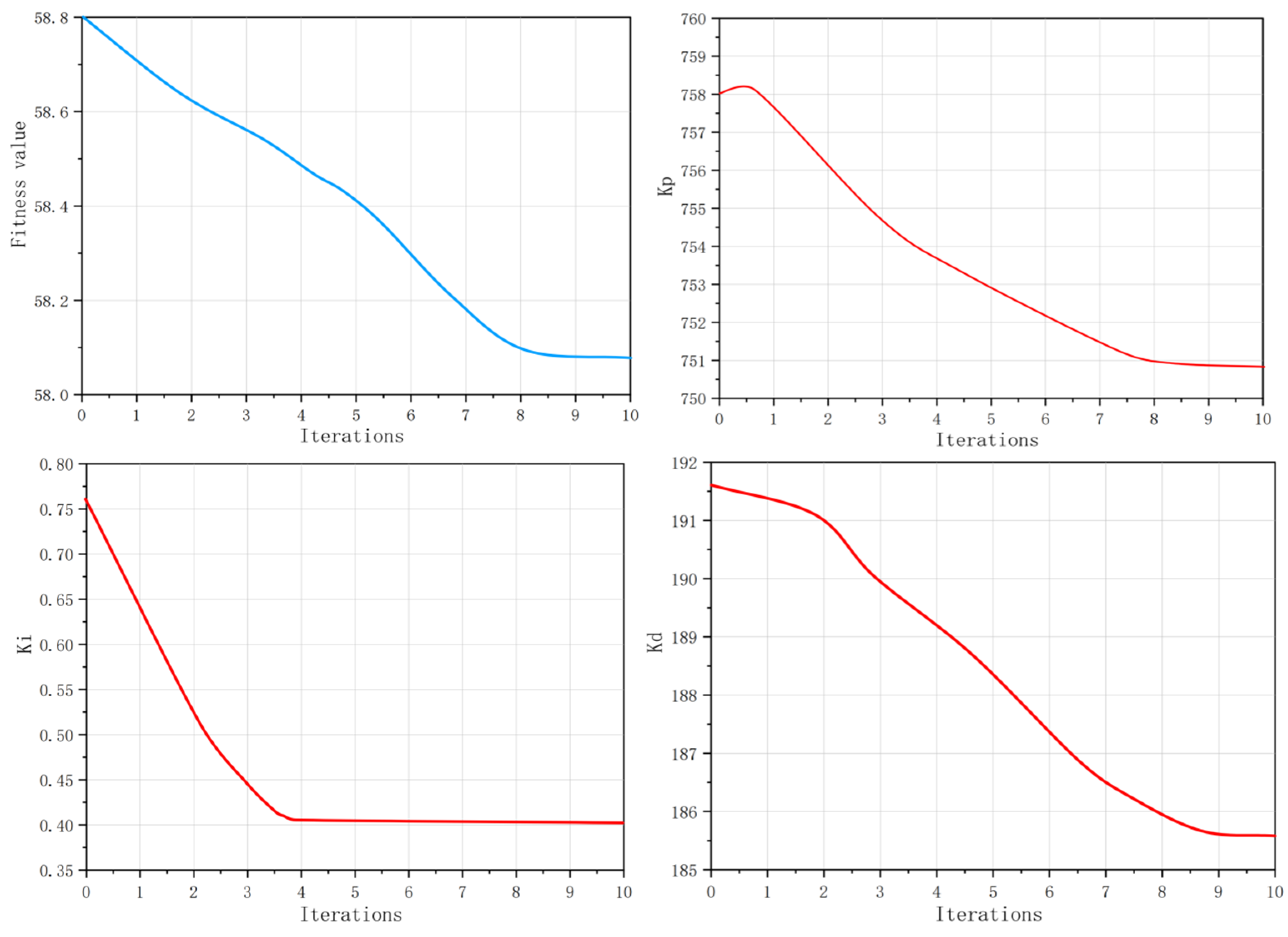
It should be noted that the PSO algorithm contains stochastic components associated with particle initialization and random search. The convergence curve shown in Figure 18 demonstrates that the global best fitness value consistently decreases and converges under the adopted parameter settings. Although only representative optimization results are presented in this study, repeated simulation runs produced similar convergence trends and controller performance. A more comprehensive statistical evaluation based on multiple independent runs and mean-standard deviation analysis will be considered in future work. The parameter variation trend during PSO optimization is shown in Figure 18.

Figure 18. Parameter variation trend.

The step response curves obtained by the optimized PSO-PID controller are shown in Figure 19:

Figure 19. PSO-PID step response curve.

Experimental Results and Analysis:

The simulation results show that the PSO-PID and FOPID further improve control performance compared with fuzzy PID. As shown in Table 10, the steady-state error is reduced to about 0.000442–0.000461 m/rad, the regulation time of the $\theta$ and $\psi$ channels is shortened to 6.35 s, and the overshoot is controlled within 0.44–1.44%, with lower IAE values of 0.42774–0.45483.

Table 10. PSO-PID step response performance.

Algorithm	Degree of Freedom	SSE	Ts/s	OS/%	IAE
PSO-PID	x	0.000442	9.35	0.442153	0.42774
	y	0.000458	9.33	0.458154	0.43578
	z	0.000461	9.38	0.457168	0.45483
	phi	0.000442	9.35	0.465473	0.42761
	theta	0.001174	6.35	1.440639	0.26314
	psi	0.001188	6.35	1.430728	0.26343

In the spiral trajectory tracking task (Table 11), the x-axis steady-state error is 0.1653 m, with IAE of 134.68 and improved tracking smoothness. However, since PSO-PID only performs offline optimization of PID parameters, it lacks real-time adaptability, resulting in limited robustness under environmental disturbances.

Table 11. PSO-PID spiral trajectory response performance.

Algorithm	Degree of Freedom	SSE	Ts/s	OS/%	IAE	ITAE
PSO-PID	x	0.1653	17.2	9.7	134.68	6643.7
	y	0.1161	14.9	7.9	118.62	6067.2
	z	0.3867	10.6	4.6	272.83	13,297.0
	phi	0.0024	4.7	7.9	1.31	67.5
	theta	0.0033	5.7	14.3	1.57	75.0
	psi	0.0028	4.8	10.7	1.33	69.0

4.2.6. Simulation Results of PSO-RBF-PID Algorithm

The PSO-RBF-PID algorithm proposed in this paper adopts the hybrid architecture of “RBF neural network + PSO global optimization + PID closed-loop control”. Through the PSO algorithm, the global collaborative optimization of RBF neural network parameters and PID initial parameters is completed offline, and the RBF neural network is used to realize online identification of the system and adaptive adjustment of PID parameters during operation [31,36,37]. It can effectively compensate for the system nonlinearity, multi-degree-of-freedom coupling and external environmental disturbances, while balancing response speed, steady-state accuracy, and system stability. The simulation design of the PSO-RBF-PID control algorithm is shown in Figure 20.

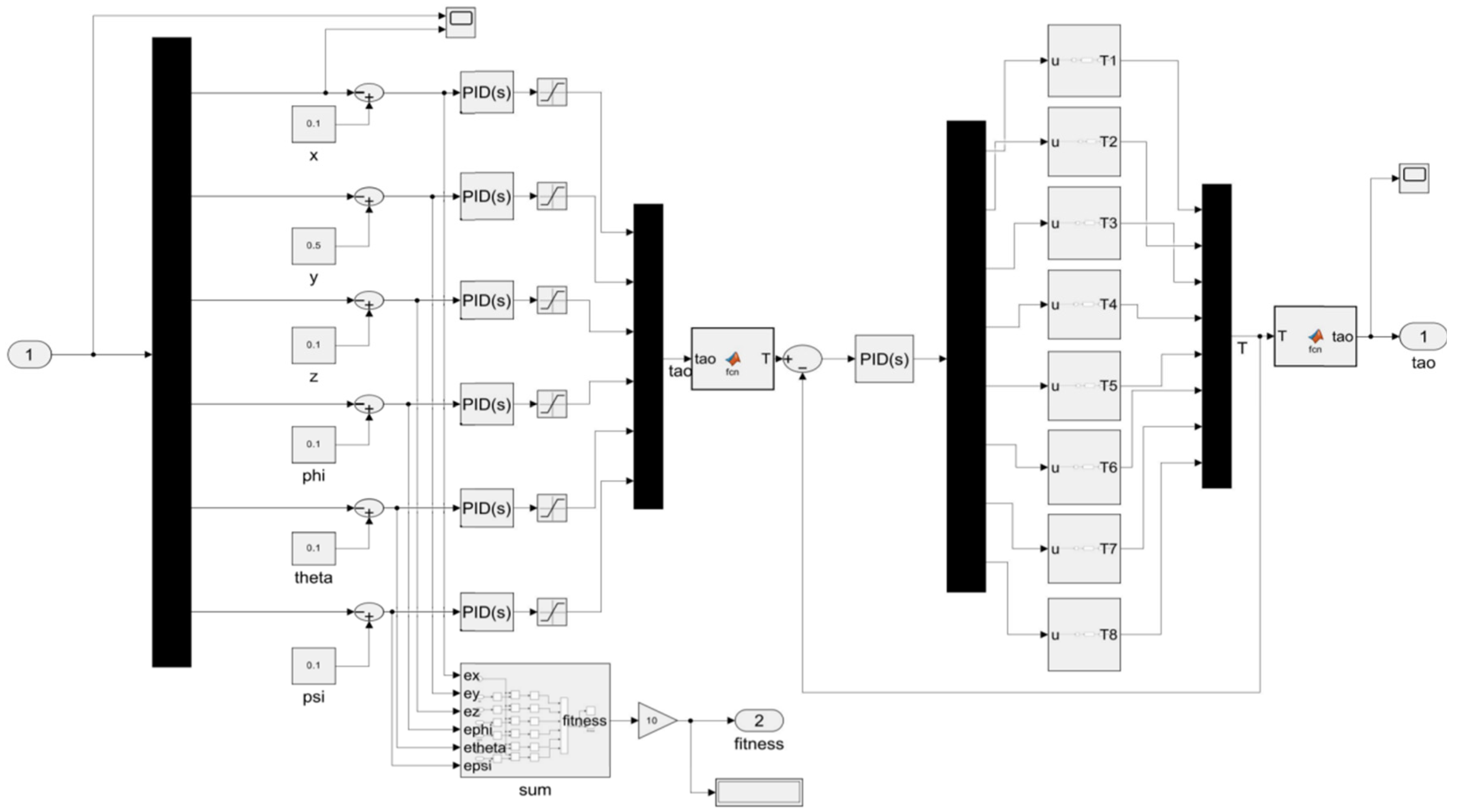
Figure 20. PSO-RBF-PID control algorithm simulation design.

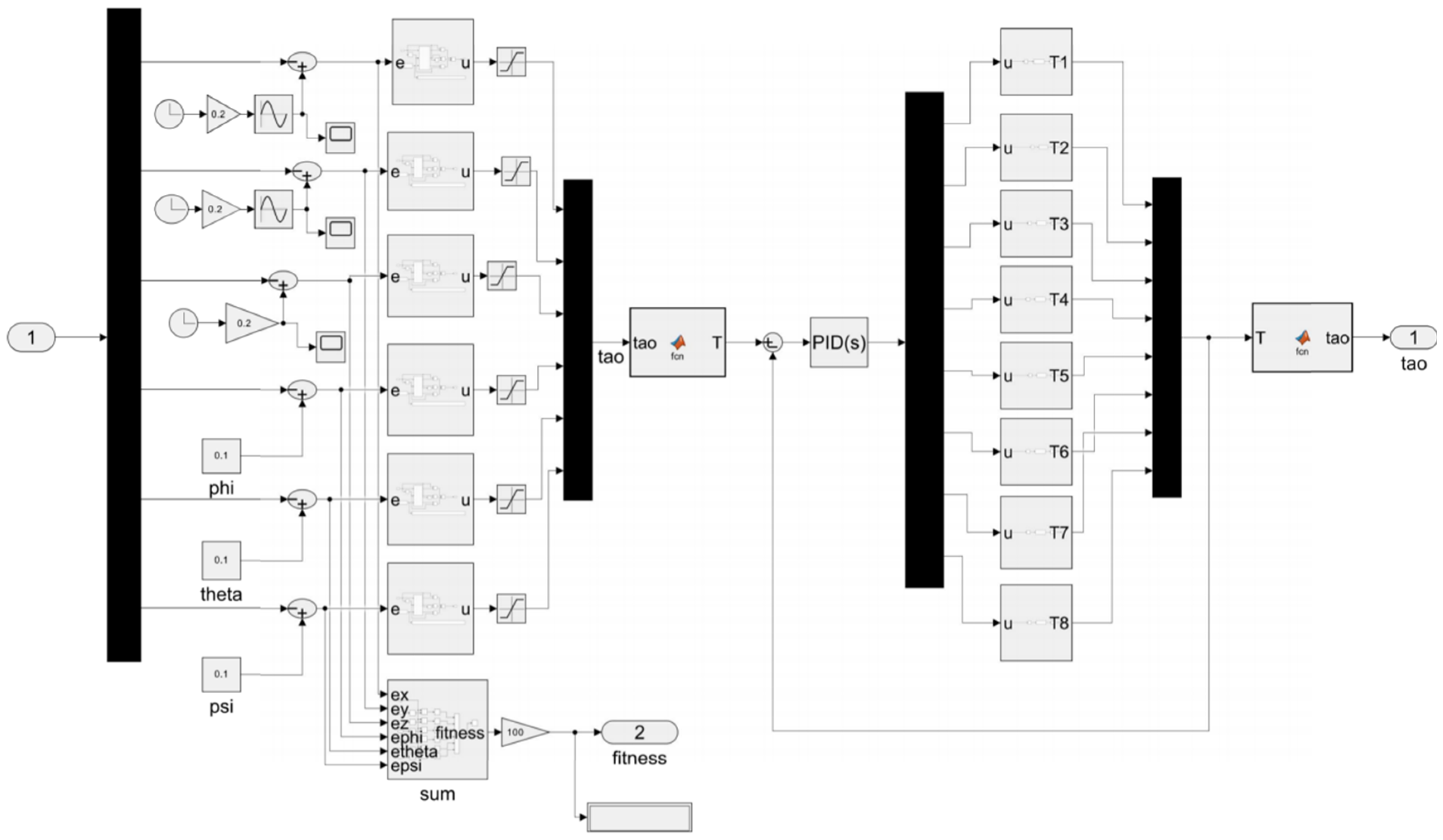
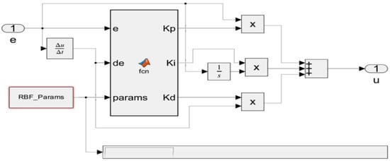
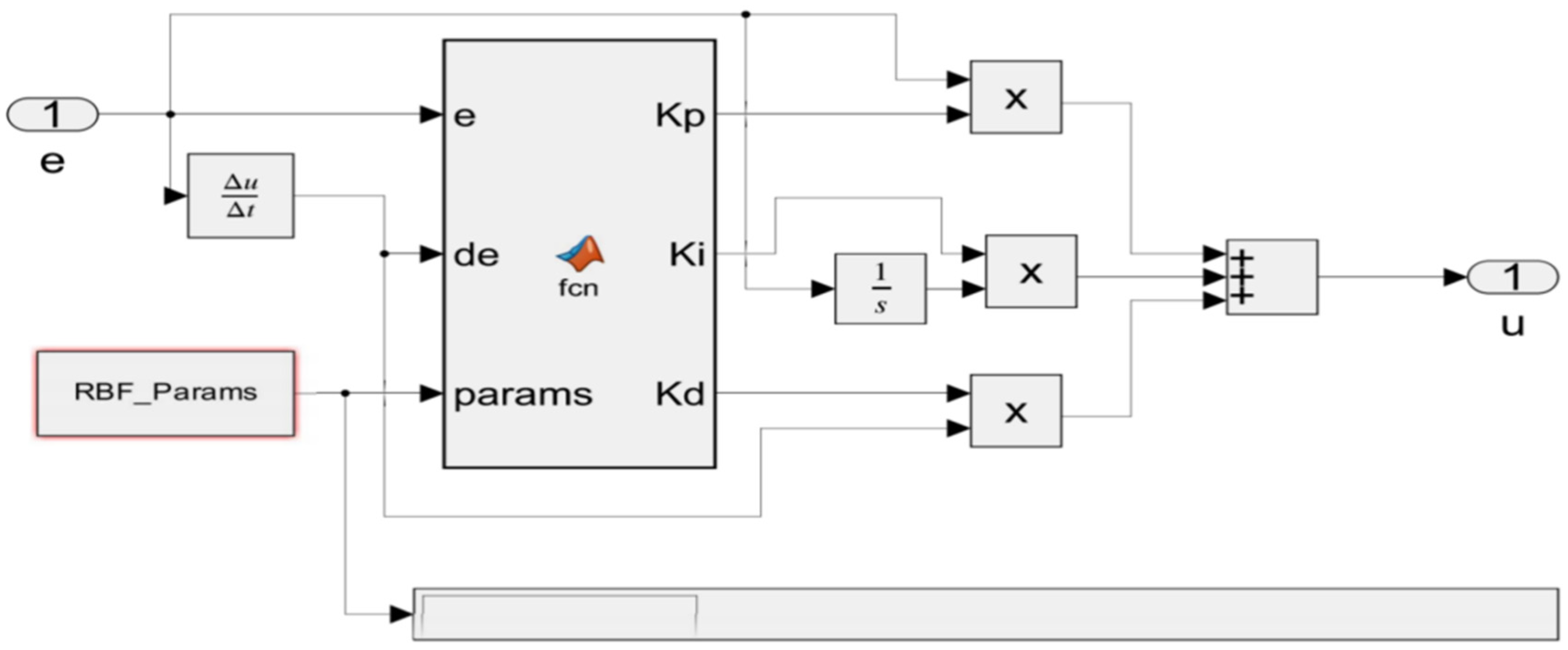
The main algorithm module of the PSO-RBF-PID simulation system is shown in Figure 21:

Figure 21. The main algorithm module of PSO-RBF-PID simulation system.

Parameter Setting:

The simulation parameters adhere to the unified benchmark settings outlined in Section 4.1. The PSO parameters, including N = 20, Tmax = 40, w = 0.7, and $c_1$ = $c_2$ = 1.49, were optimized through repeated simulations and sensitivity analysis to balance convergence speed, performance, and computational cost. Similarly, the RBF neural network parameters, with the number of hidden nodes set to 10, were determined through extensive simulations and sensitivity analysis. These parameters, along with the initial PID gains, were jointly optimized by PSO. During online operation, the RBF network adapts the PID parameters in real time to compensate for system nonlinearities and disturbances, with stability and robustness validated through multiple independent runs. The parameter changes during PSO-RBF-PID optimization and adaptation are shown in Figure 22.

Figure 22. Parameter changes.

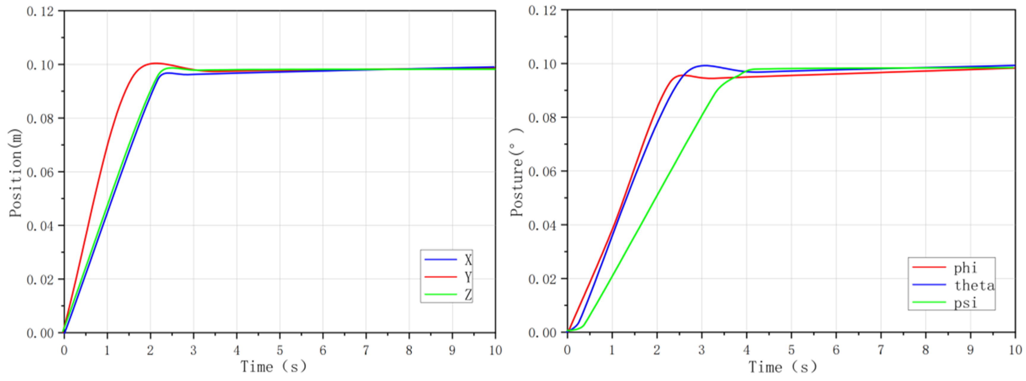
The step response curves of the PSO-RBF-PID controller are shown in Figure 23:

Figure 23. PSO-RBF-PID step response curve.

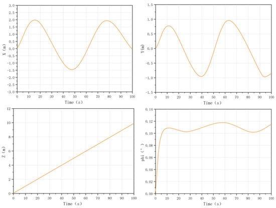
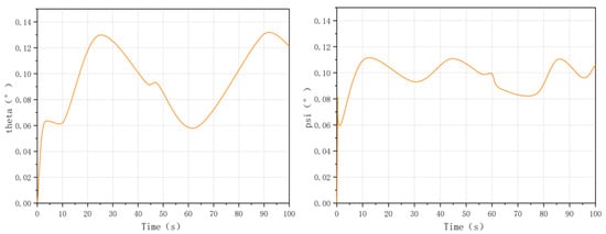
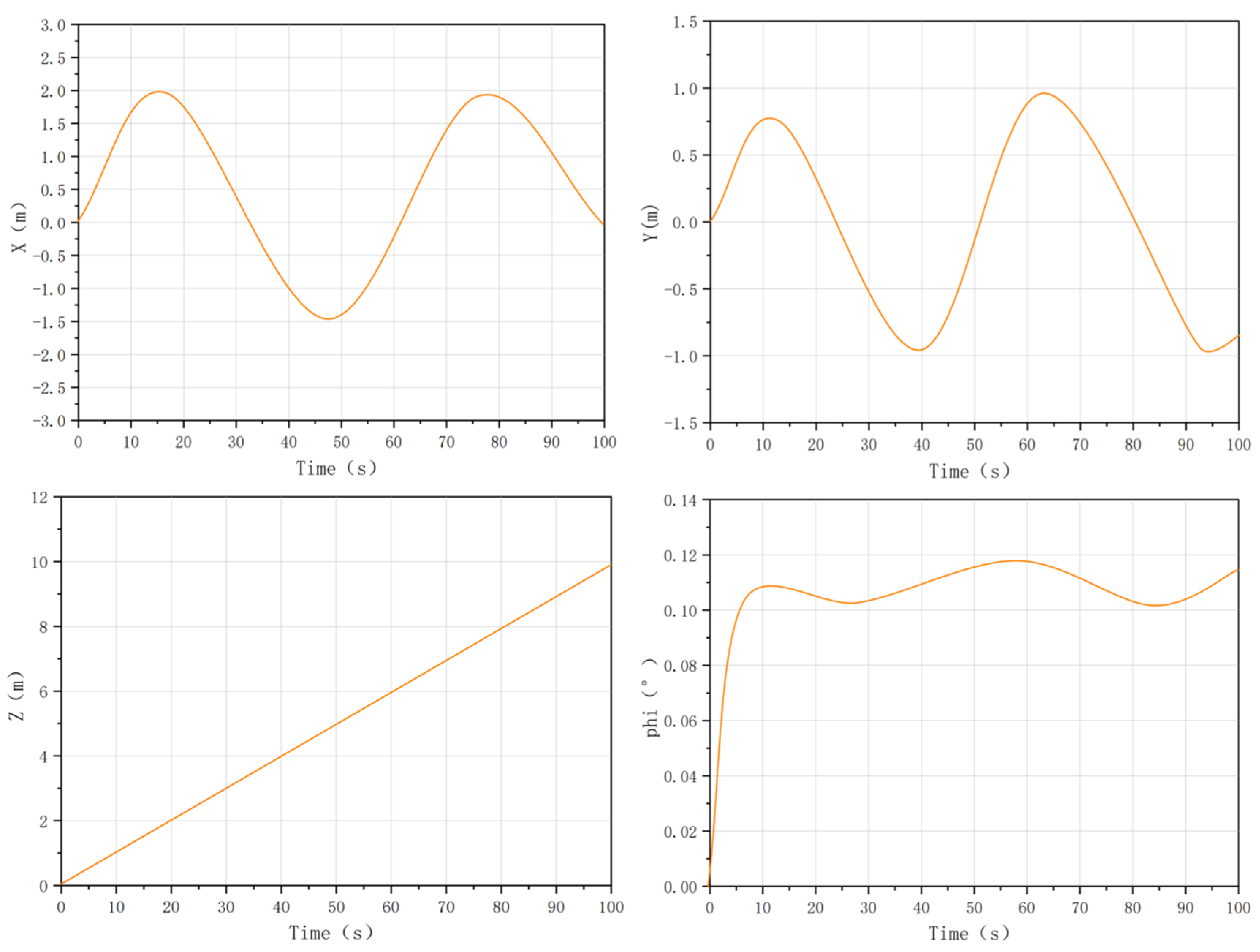
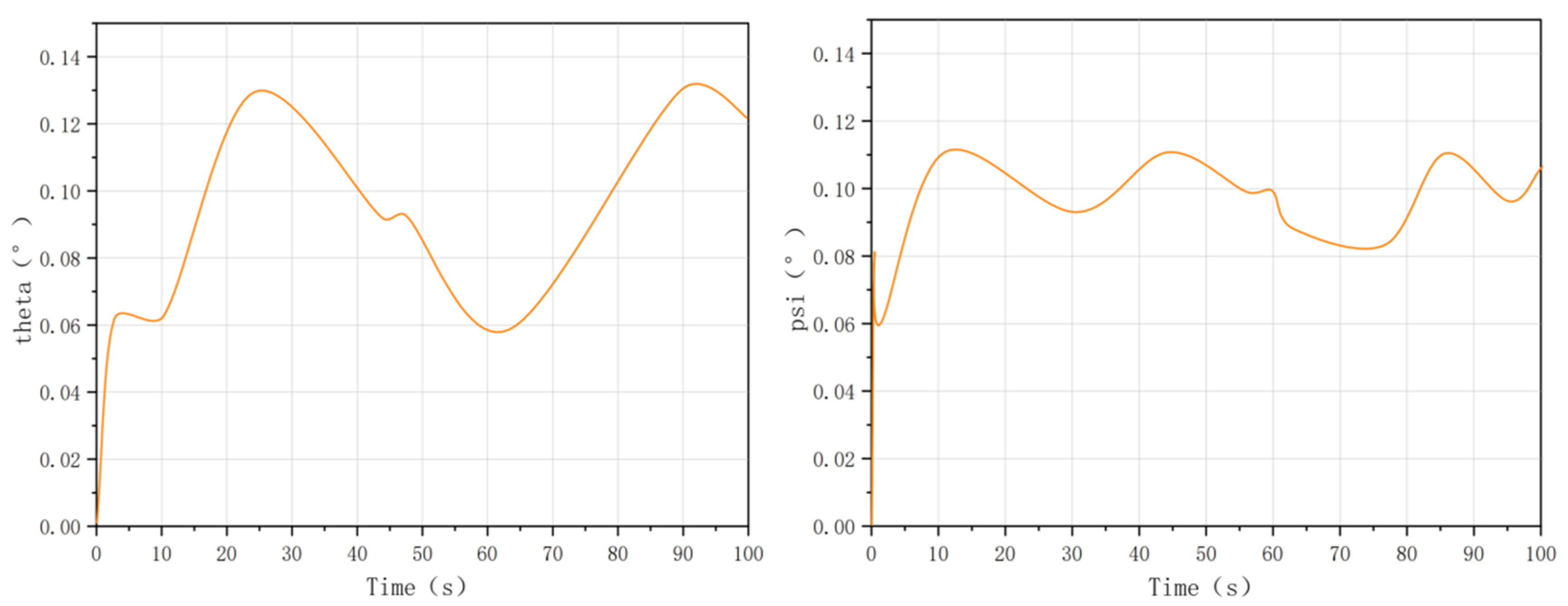
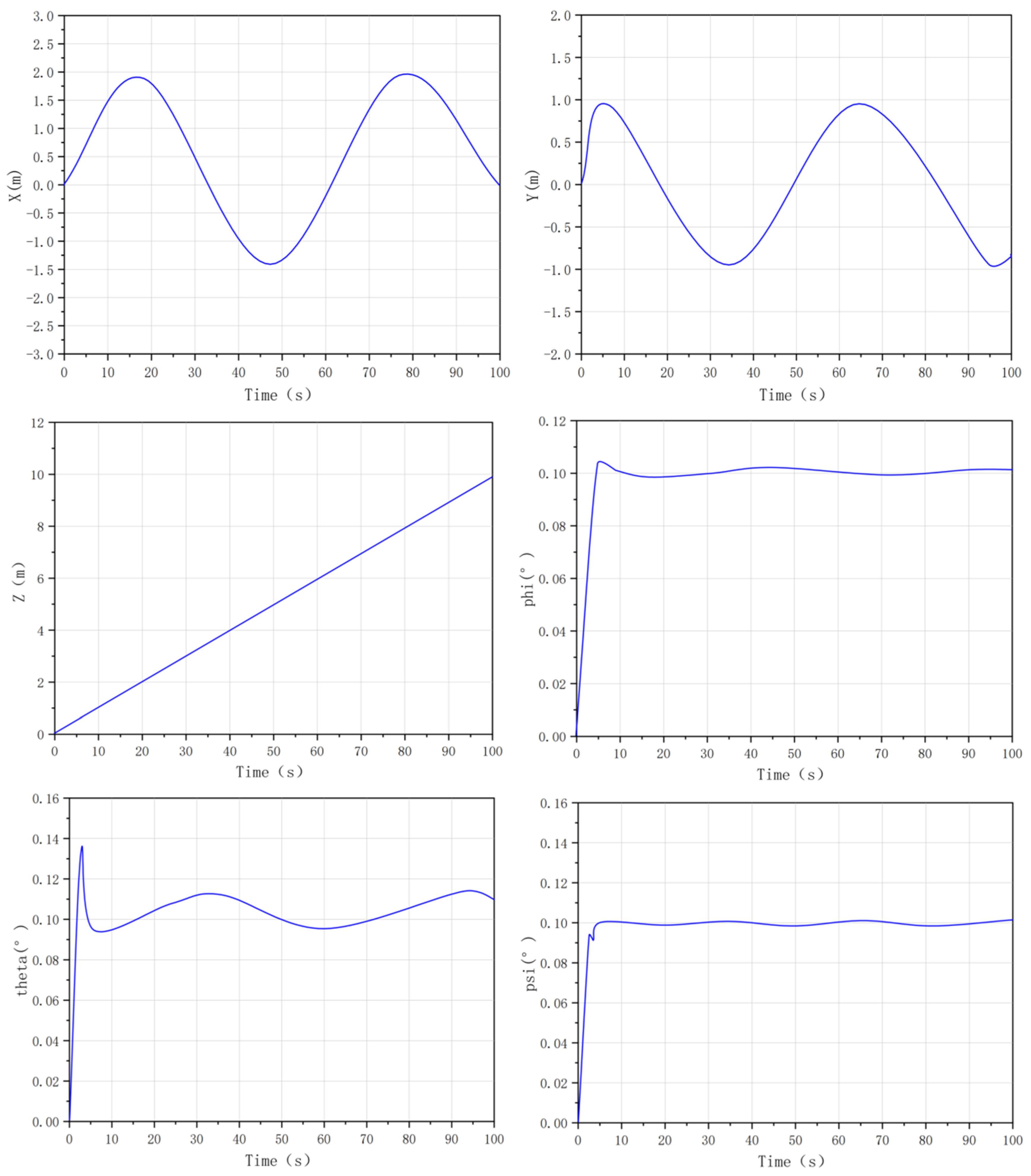
The spiral trajectory response curve of the PSO-RBF-PID controller is shown in Figure 24:

Figure 24. PSO-RBF-PID spiral trajectory response curve.

Experimental Results and Analysis:

The results demonstrate that the PSO-RBF-PID achieves superior performance in both step response and trajectory tracking tasks. As shown in Table 12, the steady-state errors of the $\theta$ and $\psi$ channels are 0.000359 and 0.000353 m/rad, respectively, with regulation times of 5.78 s and 5.83 s. Their overshoots are approximately 0.603%, and the IAE values are 0.22813 and 0.22793, indicating fast convergence and high attitude-control accuracy. Across all six degrees of freedom, the steady-state error remains within 0.000232–0.000359 m/rad, while the IAE is limited to 0.22793–0.37835, demonstrating the overall stability and accuracy of the proposed controller.

Table 12. PSO-RBF-PID step response performance.

Algorithm	Degree of Freedom	SSE	Ts/s	OS/%	IAE
PSO-RBF-PID	x	0.000347	8.55	1.625513	0.37656
	y	0.000232	8.82	1.632186	0.37645
	z	0.000356	8.38	1.623432	0.37835
	phi	0.000261	8.61	1.626738	0.37698
	theta	0.000359	5.78	0.603391	0.22813
	psi	0.000353	5.83	0.603626	0.22793

In the spiral trajectory tracking task, as shown in Table 13, the steady-state errors of the x, y, and z channels are 0.1258 m, 0.0861 m, and 0.3215 m, respectively. For the x-axis, the IAE and ITAE are 126.78 and 6271.2, respectively. The y-axis achieves the best position tracking accuracy, with a steady-state error of 0.0861 m and IAE/ITAE values of 98.56 and 4936.0. These results confirm that the PSO-RBF-PID controller provides strong dynamic tracking capability and robustness under multi-degree-of-freedom coupled conditions.

Table 13. PSO-RBF-PID spiral trajectory response performance.

Algorithm	Degree of Freedom	SSE	Ts/s	OS/%	IAE	ITAE
PSO-RBF-PID	x	0.1258	15.8	8.6	126.78	6271.2
	y	0.0861	12.5	6.4	98.56	4936.0
	z	0.3215	8.4	2.4	255.61	12,297.0
	phi	0.0013	3.6	6.1	0.88	46.1
	theta	0.0026	4.4	12.8	1.29	64.0
	psi	0.0020	3.9	8.5	0.98	48.0

4.3. Comparative Experiment

Experiment Introduction

To comprehensively and quantitatively evaluate each algorithm’s performance, this section conducts two groups of comparative experiments on a unified simulation benchmark: step response performance comparison (under ocean current interference) and spiral trajectory tracking performance comparison. The four core evaluation indicators in Section 4.1 are used for quantitative analysis, and the performance advantages of the PSO-RBF-PID algorithm proposed in this paper are verified through multi-dimensional comparison.

• Step Response Performance Comparison (Affected by variable ocean currents)

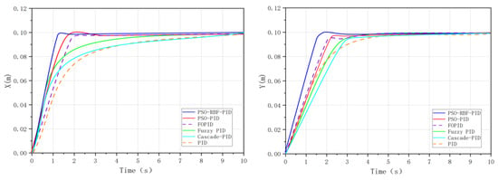
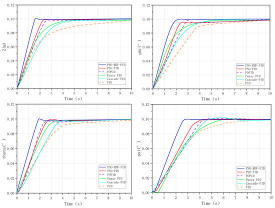
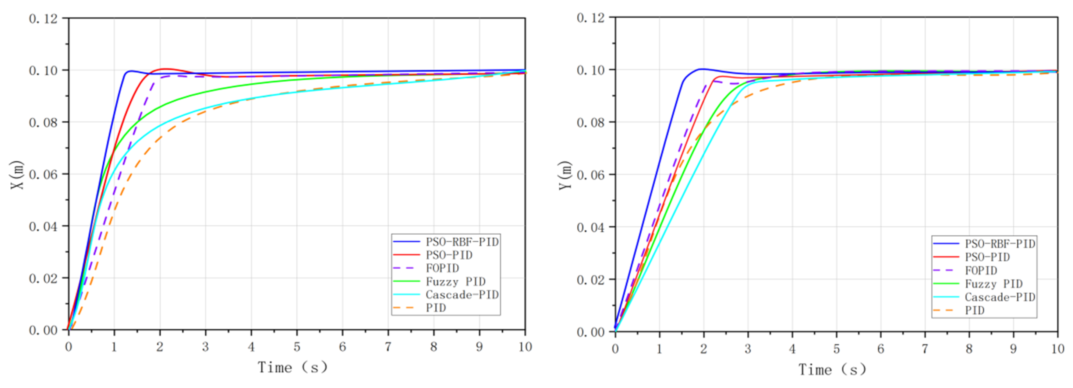
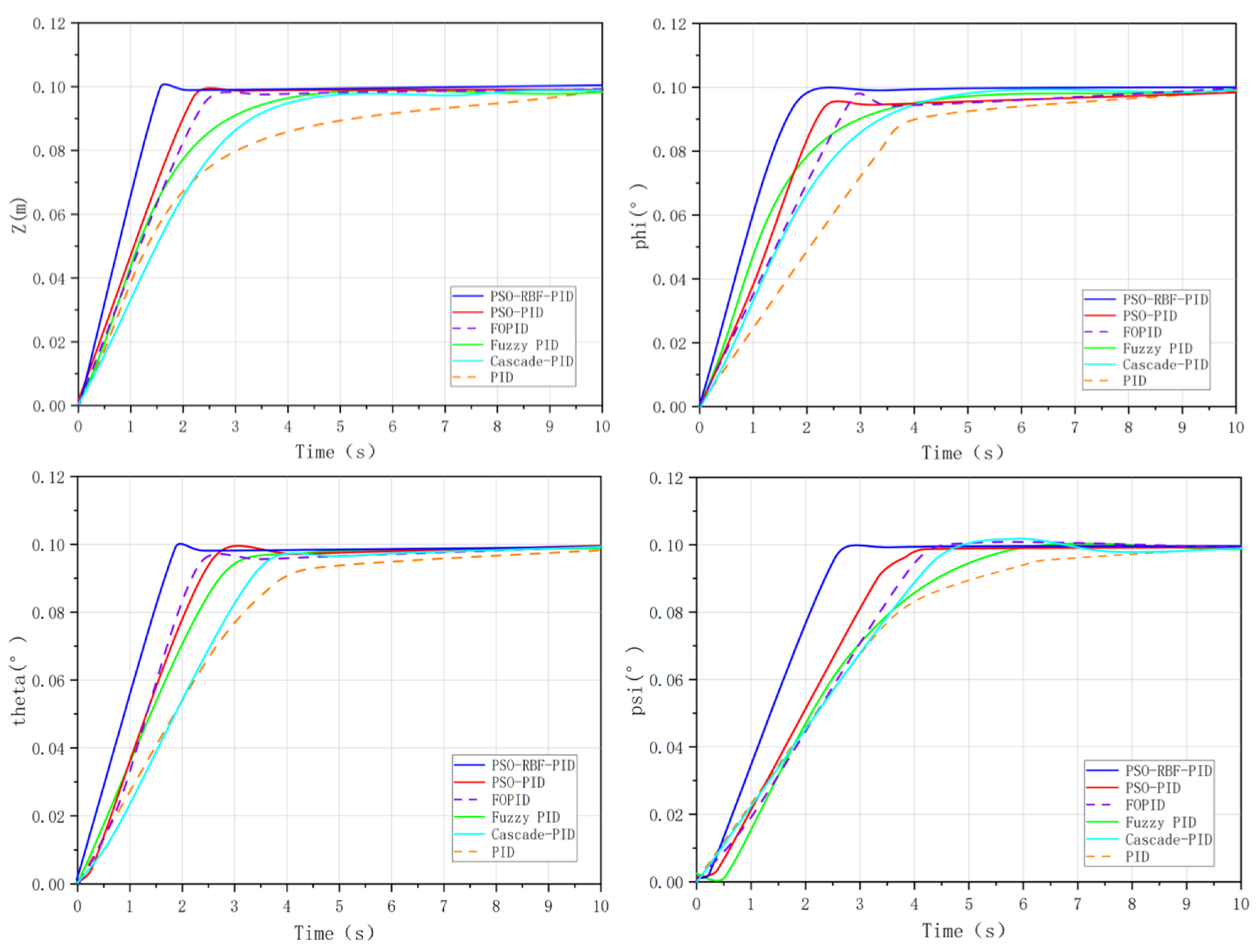
The step response results for a target value of 0.1 for six control algorithms of six channels are shown in the table of step response performance for each algorithm and Figure 25.

Figure 25. Comparative study of step responses of six control algorithms (affected by variable ocean currents).

For the conventional PID, the steady-state error of the position channels is around 0.0142–0.0152 m/rad, with a regulation time of approximately 10 s and an IAE of 0.56–0.58, indicating slow convergence. Cascade PID offers limited improvement, reducing steady-state error to 0.0135–0.0140 m/rad but increasing overshoot. Fuzzy PID significantly reduces the error to 0.0031–0.0035 m/rad and shortens the response time of $\theta$ and $\psi$. FOPID and PSO-PID further enhance control accuracy to the order of 10⁻⁴ m/rad, with faster responses and lower IAE. As summarized in the table of step response performance for each algorithm, the proposed PSO-RBF-PID achieves the smallest steady-state error, fastest convergence, and lowest IAE among all controllers. Specifically, PSO-RBF-PID results in steady-state errors of 0.000347 m (x-axis), 0.000232 m (y-axis), and 0.000356 m (z-axis), with regulation times of 8.55 s, 8.82 s, and 8.38 s, respectively, and IAE values of 0.37656, 0.37645, and 0.37835, indicating superior accuracy, speed, and efficiency [37].

2.

Anti-Interference Performance Comparison

Under a 0.2 m/s ocean current disturbance with both time-varying and sudden components, the table of step response performance for each algorithm show that the performance of conventional PID, cascade PID, and fuzzy PID degrades significantly, with increased steady-state error and overshoot. FOPID and PSO-PID exhibit improved disturbance rejection, maintaining errors at the level of 10⁻³–10⁻⁴ m/rad. In contrast, the PSO-RBF-PID maintains high accuracy and fast response under disturbance, demonstrating superior robustness due to its real-time adaptive capability. As shown in the latest data from the table of step response performance for each algorithm, the steady-state error for PSO-RBF-PID is reduced to 0.000347 m for the x-axis, 0.000232 m for the y-axis, and 0.000356 m for the z-axis, with a regulation time of 8.55 s, 8.82 s, and 8.38 s respectively, indicating its superior performance in dynamic and variable current conditions. This showcases its ability to adapt effectively to complex environmental disturbances.

3.

Spiral Trajectory Tracking Performance Comparison

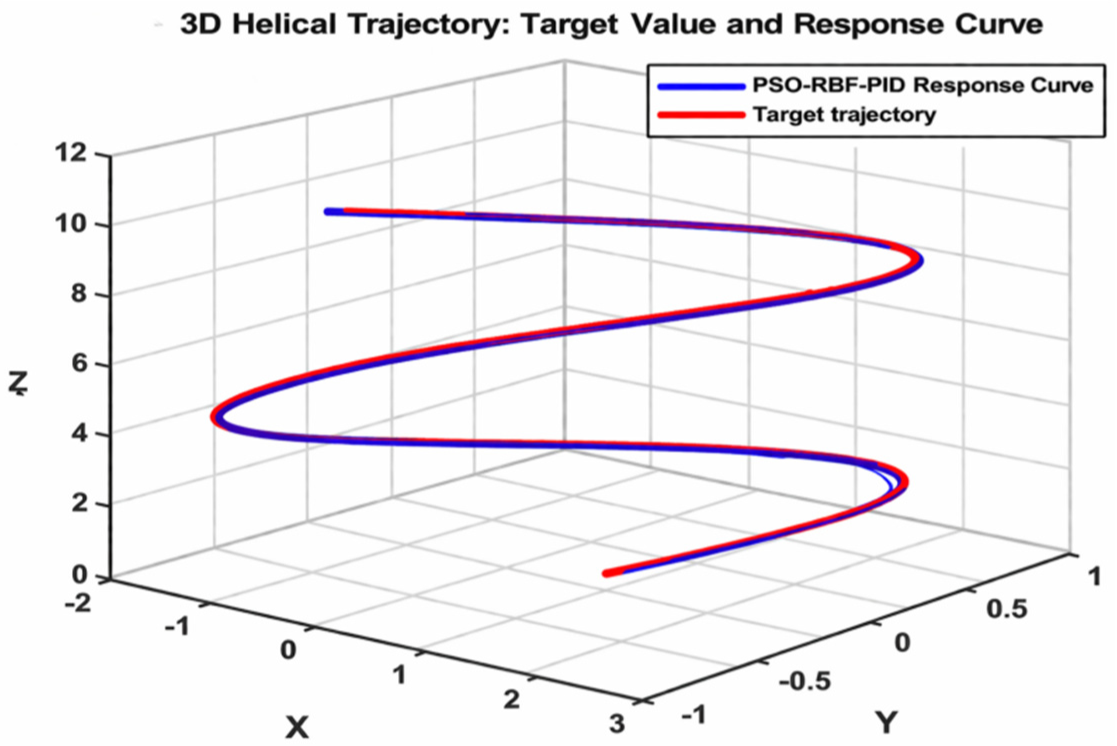
The spiral trajectory tracking performance comparison results of each algorithm are shown in the table of spiral trajectory response performance for each algorithm and illustrated in Figure 26.

Figure 26. Response comparison of spiral trajectory.

The results indicate that the PSO-RBF-PID algorithm achieves the highest trajectory tracking accuracy among all controllers. As shown in Table 3, Table 5, Table 7, Table 9, Table 11 and Table 13, the steady-state errors in the x, y, and z channels are reduced to 0.1258 m, 0.0861 m, and 0.3215 m, compared with 0.1861 m, 0.1658 m, and 0.4468 m for conventional PID. Meanwhile, the IAE and ITAE indices decrease from 134.65–286.54 and 6638.5–14,274.0 to 98.56–255.61 and 4936.0–12,297.0, respectively, indicating significantly improved tracking performance. The cascade PID shows only slight improvement over PID, with, for example, an x-axis error of 0.1813 m, while fuzzy PID reduces errors in some channels, such as the y-axis, to 0.1437 m but still suffers from dynamic lag. FOPID and PSO-PID further improve accuracy, with y-axis errors of 0.1185 m and 0.1161 m and corresponding IAE values of 122.78 and 118.62, respectively, yet they remain inferior to PSO-RBF-PID in overall response speed, tracking precision, and smoothness.

Overall, the PSO-RBF-PID achieves the smallest tracking errors, the lowest IAE/ITAE indices, and the best dynamic performance among all six controllers.

4.

Comprehensive Analysis

The above comparative experimental results fully verify that the PSO-RBF-PID algorithm proposed in this paper has the best comprehensive performance. Through the hybrid architecture of RBF neural network online identification and parameter approximation, PSO global optimization and PID closed-loop control, it effectively solves the control problems caused by the strong nonlinearity, strong coupling and environmental disturbances of underwater robots [36,37], and has significant advantages over traditional PID, fuzzy PID and PSO-PID algorithms in terms of steady-state accuracy, dynamic response speed, stability and anti-interference capability [38]. It is suitable for high-precision operation scenarios of 6-DOF multi-thruster underwater robots in complex marine environments.

Although the simulation considers hydrodynamic disturbances, actuator saturation, parameter uncertainty, sensor noise, and time delay, it cannot fully reproduce real underwater conditions. Practical operation may involve more complex fluid–structure interactions, turbulent currents, actuator degradation, sensor drift, and communication delays. Therefore, the present results only demonstrate the relative performance of the proposed controller in a controlled simulation case study. Future work will involve water-tank or real underwater robot experiments to further validate its practical applicability.

5. Conclusions

This paper proposes a PSO-RBF-PID controller for the considered 6-DOF multi-thruster underwater robot under nonlinear dynamics, strong coupling, and environmental disturbances. Based on a simplified dynamic model with external disturbance scenarios, comparative simulations were conducted with PID, cascade PID, fuzzy PID, FOPID, and PSO-PID controllers. The results show that the proposed method improves global parameter search by jointly optimizing the initial PID gains and RBF network parameters, while the RBF-based online adaptive mechanism enhances disturbance compensation and robustness. In the step-response task, the steady-state error was reduced to 0.000347–0.000356 m/rad, the settling time was shortened to 5.78–8.55 s, and the IAE values were reduced to 0.22793–0.37656. In the helical trajectory-tracking task, the x-axis tracking error was reduced to 0.1258 m, with lower IAE and ITAE values of 126.78 and 6271.2, respectively, demonstrating improved tracking accuracy and stability. Unlike FOPID, the proposed method does not rely on fractional-order approximation but improves adaptability through online RBF-based PID gain correction. Overall, under the same simulation conditions, PSO-RBF-PID achieved the best overall performance in precision, response speed, and robustness among the compared controllers. However, the current validation is limited to simulation results based on a simplified dynamic model and predefined disturbance scenarios. Real underwater environments may involve more complex hydrodynamic effects, actuator dynamics, sensor noise, and communication delays. Future work will therefore focus on real-time implementation, hardware-resource evaluation, more realistic disturbance modeling, and experimental validation using a physical underwater robot platform [31,39,40].

References

- Liu, X.; Zhang, Y.; Wang, J. Adaptive Attitude Control of Underwater Robots Based on Improved Sliding Mode Theory. Ocean Eng. 2023, 289, 116023. [Google Scholar] [CrossRef] [Scilit]
- Liu, K.; Ding, M.; Pan, B.; Yu, P.; Lu, D.; Chen, S.; Zhang, S.; Wang, G. A Maneuverable Underwater Vehicle for Near-Seabed Observation. Nat. Commun. 2024, 15, 10284. [Google Scholar] [CrossRef] [Scilit] [PubMed]
- Chen, M.; Wang, T.; Zhang, H. Parameter Design and Hydrodynamic Analysis of Screw Propellers for Port Underwater Dredging Robots. Ocean Eng. 2024, 298, 117245. [Google Scholar] [CrossRef] [Scilit]
- Huang, Y.; Chen, Z.; Li, L. Hovering Control of Underwater Robots Using Improved PID with Nonlinear Disturbance Observer. Control Eng. Pract. 2023, 140, 105689. [Google Scholar] [CrossRef] [Scilit]
- Gao, X.; Hu, X.; Liu, J.; Li, T. Event-Driven Prescribed Optimal Disturbance Rejection for Dynamic Positioning of Ships via Reinforcement Learning. IEEE Trans. Autom. Sci. Eng. 2026, 23, 4615–4626. [Google Scholar] [CrossRef] [Scilit]
- Wang, J.; Yan, S.; Bao, H.; Chen, C.; Yu, D.; Li, J.; Chen, X.; Dou, R.; Tang, Y.; Li, S. Reinforcement-Learning-Based Adaptive PID Depth Control for Underwater Vehicles Against Buoyancy Variations. J. Mar. Sci. Eng. 2026, 14, 323. [Google Scholar] [CrossRef] [Scilit]
- Amare, N.D.; Yang, S.J.; Son, Y.I. An Optimized Position Control via Reinforcement-Learning-Based Hybrid Structure Strategy. Actuators 2025, 14, 199. [Google Scholar] [CrossRef] [Scilit]
- Chen, Q.; Cheng, Y.; Yuan, Y.; Hua, L. Autonomous Navigation of an Unmanned Underwater Vehicle via Safe Reinforcement Learning and Active Disturbance Rejection Control. J. Mar. Sci. Eng. 2026, 14, 425. [Google Scholar] [CrossRef] [Scilit]
- Cao, L.; Qin, Y.; Pan, Y.; Liang, H. Prescribed Performance-Based Optimal Formation Control for USVs With Position Constraints and Yaw Angle Time-Varying Partial Constraints. IEEE Trans. Intell. Transp. Syst. 2025, 26, 4109–4121. [Google Scholar] [CrossRef] [Scilit]
- Algarín-Pinto, J.A.; Garza-Castañón, L.E.; Vargas-Martínez, A.; Minchala-Ávila, L.I.; Payeur, P. Intelligent Motion Control to Enhance the Swimming Performance of a Biomimetic Underwater Vehicle Using Reinforcement Learning Approach. IEEE Access 2025, 13, 37128–37146. [Google Scholar] [CrossRef] [Scilit]
- Luo, G.; Zhang, D.; Feng, W.; Jiang, Z.; Liu, X. Deep Reinforcement Learning Based Active Disturbance Rejection Control for ROV Position and Attitude Control. Appl. Sci. 2025, 15, 4443. [Google Scholar] [CrossRef] [Scilit]
- Huang, X.; Chen, Y.; Zhan, W.; Lin, J.; Zhang, Y. Motion Control of Robotic Fish Based on BP Neural Network-Fuzzy Fusion Optimization Algorithm. IEEJ Trans. Electr. Electron. Eng. 2026; early view. [CrossRef] [Scilit]
- Liang, Y. Robot Trajectory Tracking Control Based on Neural Networks and Sliding Mode Control. IEEE Access 2025, 13, 96740–96757. [Google Scholar] [CrossRef] [Scilit]
- Huerta-Moro, S.; Tlelo-Cuautle, E. Parasitic Resistance and Circuit Variation Effects in a DC–DC Buck Converter With Integer/Fractional-Order PID Controllers. Int. J. Circuit Theory Appl. 2025, 54, 2314–2321. [Google Scholar] [CrossRef] [Scilit]
- Zhang, P.; Hao, L.; Wang, R. Adaptive Transmission Interval-Based Self-Triggered Model Predictive Control for Autonomous Underwater Vehicles with Additional Disturbances. J. Mar. Sci. Eng. 2024, 12, 1489. [Google Scholar] [CrossRef] [Scilit]
- Zhao, Y.; Xu, S.; Zheng, X.; Luo, L.; Xu, B.; Xiong, C. Enhanced Real-Time Simulation of ROV Attitude and Trajectory Under Ocean Current and Wake Disturbances. Appl. Syst. Innov. 2025, 8, 75. [Google Scholar] [CrossRef] [Scilit]
- Yang, F.; Wang, G.; Zhang, C. Hydrodynamic Performance and Motion Control of Remotely Operated Vehicles in Current Environments. Ocean Eng. 2023, 291, 116312. [Google Scholar] [CrossRef] [Scilit]
- Zhang, D.; Zhao, B.; Zhang, Y.; Zhou, N. Numerical Simulation of Hydrodynamics of Ocean-Observation-Used Remotely Operated Vehicle. Front. Mar. Sci. 2024, 11, 1357144. [Google Scholar] [CrossRef] [Scilit]
- Lee, K.; Kim, J.; Park, S. Design of an Underwater Observation Robot for Ship Inspection. Ocean Eng. 2024, 302, 117568. [Google Scholar] [CrossRef] [Scilit]
- Fan, S.; Wang, H.; Zuo, C.; Han, J. Fuzzy Adaptive PID-Based Tracking Control for Autonomous Underwater Vehicles. Actuators 2025, 14, 470. [Google Scholar] [CrossRef] [Scilit]
- Rojas-Galván, R.; Mercado-Gutiérrez, E.; Tlelo-Cuautle, E. Optimizing Chaotic Systems by Orbit Counting and Fourier Spectrum: FPGA Implementation and Image Encryption Application. Math. Model. Anal. 2025, 30, 322–341. [Google Scholar] [CrossRef] [Scilit]
- Wang, Y.; Hou, Y.; Lai, Z.; Cao, L.; Hong, W.; Wu, D. An Adaptive PID Controller for Path Following of Autonomous Underwater Vehicle Based on Soft Actor–Critic. Ocean Eng. 2024, 307, 118171. [Google Scholar] [CrossRef] [Scilit]
- Zhang, W.; Wu, W.; Li, Z.; Du, X.; Yan, Z. Three-Dimensional Trajectory Tracking of AUV Based on Nonsingular Terminal Sliding Mode and Active Disturbance Rejection Decoupling Control. J. Mar. Sci. Eng. 2023, 11, 959. [Google Scholar] [CrossRef] [Scilit]
- Wang, G.; Li, Y.; Zhang, H. Design of Underwater Robot Control System Based on Fuzzy Shared Control. Ocean Eng. 2024, 305, 117892. [Google Scholar] [CrossRef] [Scilit]
- Wang, P.; Liu, X.; Song, A. Actuation and Locomotion of Miniature Underwater Robots: A Survey. Engineering 2025, 51, 206–227. [Google Scholar] [CrossRef] [Scilit]
- Bashir, A.; Khan, S.; Iqbal, N.; Bashmal, S.; Ullah, S.; Usman, M. A Review of Various Control Algorithms for Unmanned Underwater Vehicle Trajectory Control. Sustainability 2023, 15, 14691. [Google Scholar] [CrossRef] [Scilit]
- Yan, J.; Zhang, T.; Guan, X.; Yang, X.; Chen, C. Digital Twin-Driven Swarm of Autonomous Underwater Vehicles for Marine Exploration. Commun. Eng. 2026, 5, 18. [Google Scholar] [CrossRef] [Scilit] [PubMed]
- Bai, F.; Song, X.; Wang, Z.; Wang, X.; Liu, Y.; Liu, K.; Xue, G. Research on Design, Modeling, and Maneuverability of Hybrid-Driven Bionic Underwater Robots. Front. Mar. Sci. 2025, 12, 1648335. [Google Scholar] [CrossRef] [Scilit]
- Dong, J.; Duan, X. A Robust Control via a Fuzzy System with PID for the ROV. Sensors 2023, 23, 821. [Google Scholar] [CrossRef] [Scilit] [PubMed]
- Duan, Y.; Xiang, X.; Liu, C.; Yang, L. Double-Loop LQR Depth Tracking Control of Underactuated AUV: Methodology and Comparative Experiments. Ocean Eng. 2024, 300, 117410. [Google Scholar] [CrossRef] [Scilit]
- Zhang, B.; Li, Y.; Chen, J. Particle Swarm Optimization for PID Parameter Tuning in Underwater Robot Control. Ocean Eng. 2023, 287, 115897. [Google Scholar] [CrossRef] [Scilit]
- Chen, H.; Li, W.; Liu, Z. Fuzzy PID Algorithm for Underwater Robot Control System Optimization. Ocean Eng. 2024, 293, 116789. [Google Scholar] [CrossRef] [Scilit]
- Zhang, P.; Chen, J.; Xia, H.; Li, Z.; Lin, X.; Zhou, P. Development and Motion Mechanism of a Novel Underwater Exploration Robot for Stratum Drilling. IEEE J. Ocean. Eng. 2024, 49, 763–774. [Google Scholar] [CrossRef] [Scilit]
- Vangi, M.; Topini, E.; Liverani, G.; Topini, A.; Ridolfi, A.; Allotta, B. Design, Development, and Testing of an Innovative Autonomous Underwater Reconfigurable Vehicle for Versatile Applications. IEEE J. Ocean. Eng. 2025, 50, 509–526. [Google Scholar] [CrossRef] [Scilit]
- Yang, C.; Liu, S.; Su, H.; Zhang, L.; Xia, Q.; Chen, Y. Review of Underwater Adsorptive-Operating Robots: Design and Application. Ocean Eng. 2024, 294, 116794. [Google Scholar] [CrossRef] [Scilit]
- Gong, Q.; Zhang, W.; Zhang, H.; Yang, H.; Sun, R. An Underwater Dual-Mode Robot with Simultaneous Swimming and Crawling Functions: Design and Experiment. Ocean Eng. 2024, 309, 118349. [Google Scholar] [CrossRef] [Scilit]
- Li, Z.; Gai, Q.; Lei, M.; Yan, H.; Xia, D. Development of a Multi-Tentacled Collaborative Underwater Robot for Biomimetic Propulsion. Ocean Eng. 2024, 308, 118376. [Google Scholar] [CrossRef] [Scilit]
- Yang, Z.; Lang, Q.; Xiong, Y.; Yang, S.; Zhang, C.; Deng, L.; Zhang, D. Research on Trajectory Tracking Control Method for Crawler Robot Based on Improved PSO Sliding Mode Disturbance Rejection Control. Sensors 2025, 25, 2113. [Google Scholar] [CrossRef] [Scilit] [PubMed]
- Guo, J.; Wang, J.; Bo, Y. An Observer-Based Adaptive Neural Network Finite-Time Control for Autonomous Underwater Vehicles. Drones 2023, 7, 604. [Google Scholar] [CrossRef] [Scilit]
- Ahmad, A.; Yushchenko, A. Neural Network-Based Control of an Undulating Robot for Underwater Pipeline Tracking in Unity 3D. In Proceedings of the 2025 7th International Youth Conference on Radio Electronics, Electrical and Power Engineering (REEPE), Moscow, Russia, 8–10 April 2025; pp. 1–6. [Google Scholar] [CrossRef] [Scilit]
Disclaimer/Publisher’s Note: The statements, opinions and data contained in all publications are solely those of the individual author(s) and contributor(s) and not of MDPI and/or the editor(s). MDPI and/or the editor(s) disclaim responsibility for any injury to people or property resulting from any ideas, methods, instructions or products referred to in the content. |
© 2026 by the authors. Licensee MDPI, Basel, Switzerland. This article is an open access article distributed under the terms and conditions of the Creative Commons Attribution (CC BY) license.