Admittance Prediction for PMSG via Dimensionality-Reduced Equivalent Circuits and Support Vector Machines

Abstract

Admittance-based analysis of wind farm-integrated power systems is inaccurate across varying operating points (OPs) resulting from wind speed fluctuations and shifting grid conditions. Existing methods can be classified as model-driven, which require detailed system modeling and struggle with parameter extraction, and as data-driven, which often lack physical interpretability, suffer from high dimensionality, and provide insufficient coverage of training frequency points. This study introduces an AM reconstruction framework that integrates equivalent circuits with a support vector machine (SVM). The approach first applies vector fitting and an equivalent-circuit transformation to decompose the admittance response into first- and second-order subcircuits, thereby representing the frequency-domain characteristics with low-dimensional, more physically interpretable parameters. Subsequently, an SVM establishes a nonlinear mapping between OPs and equivalent-circuit parameters, enabling the reconstruction of continuous admittance transfer functions for new OPs. This framework transforms the modeling of high-dimensional frequency-domain data into a low-dimensional physical parameter prediction problem, thereby avoiding error accumulation from interpolation over discrete frequency points. The proposed method is validated using a direct-drive permanent magnet synchronous generator (PMSG) wind turbine model connected to the IEEE 14-bus test system. Frequency-domain simulations and error analyses under previously unseen OPs confirm the method’s high prediction accuracy and strong generalization capability.

1. Introduction

Wind power capacity has grown rapidly in recent years. During this period, direct-drive permanent magnet synchronous generator (PMSG) systems have been extensively deployed due to their high efficiency and reliability [1,2,3]. However, most wind farms are typically located far from major load centers and connected to the grid via long-distance transmission lines. This configuration intensifies control and electromagnetic coupling between wind farms and the external grid, thereby increasing the risk of wideband oscillations [4,5].

The black-box nature of practical equipment stems from incomplete information about control structures and parameters. This limitation has led to widespread adoption of admittance-based analysis to investigate instability issues [6,7]. This approach requires both equivalent grid admittance and PMSG output admittance at a specific operating point (OP). However, stochastic variability in wind speed and fluctuations in dispatch power commands cause wind farms to operate over a broad range of conditions [8]. As a result, small-signal stability characteristics can vary widely within a high-dimensional operating space [9]. Mainstream methods for admittance acquisition, such as analytical derivations and frequency-domain scanning measurements [10,11,12,13], typically produce models that are valid only near a single steady-state OP [14]. Thus, stability assessment requires repeated admittance identification at various operating points. This process is time-consuming, hard to extend over the entire region, and insufficient for comprehensive risk screening [15]. To address the operating-point dependence of admittance models (AM), previous studies have explored multiple approaches to develop generalized models that are robust across a range of OPs. These approaches fall into two broad categories: analytical-model-based and data-driven methods.

For analytical model-based methods, representative strategies have been reported in [16,17,18]. In [16], an approximately decoupled sequence-domain AM was developed for grid-following inverters (GFLIs); however, this method relies on the phase-locked loop (PLL) and does not apply to PLL-less grid-forming inverters (GFMIs). In [17], an improved decoupled AM of inverter-based resources (IBRs) in the synchronous reference frame was proposed. Although applicable to both GFL and GFM converters, it involves complex calculations and multiple matrix inversions, resulting in a relatively high computational burden and requiring at least 28 data points. In [18], a 2 × 2 frequency-coupled admittance matrix was established in the sequence domain to describe the coupling between subsynchronous and complementary supersynchronous frequencies simultaneously; however, it still fundamentally relies on equivalent modeling and several simplifying assumptions.

With the rapid development of data-driven techniques, machine learning has been increasingly used to address nonlinear operating uncertainties in grid-connected microgrids, such as forecasting, clustering, and energy management [19], and has also attracted growing attention for admittance prediction under varying OPs [20,21,22,23,24,25,26,27,28,29,30]. These methods use trained models to predict the admittance at unseen operating points. In [20], a recurrent neural network (RNN)-based method was proposed for measuring converter admittance, but it was limited to specific operating conditions. In [21], an artificial neural network (ANN) was employed to predict AMs under different operating conditions. Transfer-learning-based admittance prediction methods for two-level and modular multilevel converters were proposed in [22,23], both of which require offline data generation followed by online admittance identification. In [24,25], small-scale feedforward neural networks (FNNs) combined with transfer learning were used for admittance prediction; however, the overall procedure remains relatively complicated due to the need for pretraining and transfer learning. In [26], a physics-informed neural network (PINN)-based method was proposed for predicting the admittance of IBRs. Although it reduces the computational burden of online admittance identification, it still requires both offline and online training, relies on prior knowledge of the converter control structure, and has been validated only for current-controlled grid-following inverters. In [27], support vector machines (SVMs) were extended to admittance prediction for both grid-following and grid-forming converters. In [28], the Drop-KAN architecture was introduced into power electronics and shown to maintain high prediction accuracy across voltage-source-converter systems with different topologies without reconfiguring the network architecture. In [29], a transfer-learning-based data-driven method was proposed for identifying the admittance of doubly fed induction generators (DFIGs) under multiple operating conditions, providing an effective solution for small-sample scenarios through tailored operating-condition clustering, physics-informed feature selection, and maximum mean discrepancy (MMD)-based domain adaptation. In [30], frequency-coupled admittance measurements were combined with vector fitting (VF) and a polytopic modeling framework, thereby requiring only three to five local models, significantly reducing measurement effort, data volume, and model complexity.

In summary, analytical model-based methods provide clear physical interpretability but require dedicated derivations tailored to specific control structures and operating mechanisms. Consequently, these methods involve cumbersome modeling procedures, a strong reliance on prior knowledge, and a challenging tradeoff between accuracy and complexity, particularly in frequency-coupled and wide-operating-range scenarios. In contrast, data-driven methods circumvent the complexity of mechanism-based modeling and offer greater flexibility for predicting admittance across multiple operating points. However, current data-driven approaches generally lack physical interpretability, depend on high-dimensional admittance data, incur substantial offline acquisition costs, and demonstrate limited generalization. They are typically trained on discrete frequency points, which restricts frequency coverage.

To address these challenges, this paper introduces an admittance-model reconstruction framework that merges equivalent-circuit transformation with data-driven prediction. First, a vector fitting (VF)-based equivalent-circuit transformation method is developed for the PMSG to characterize its AM. By extracting equivalent-circuit element parameters, such as resistances, inductances, capacitances, and controlled sources, this approach reduces the dimensionality of frequency-domain admittance data. Second, a support vector machine (SVM) is used to predict these low-dimensional parameters. This enables the establishment of a generalized $dq$ frame AM for black-box systems across a wide range of operating points, including nonconventional grid conditions. The key distinction is that the proposed method does not directly learn admittance samples at discrete frequencies; instead, it learns the operating-point dependence of physically interpretable circuit parameters extracted from a rational admittance representation. The main contributions of this paper are as follows.

• An equivalent-circuit transformation framework for PMSG admittance modeling is proposed, mapping the system into first- and second-order subcircuits.
• A data-driven SVM-based prediction strategy is developed to map varied grid conditions to low-dimensional equivalent-circuit parameters directly.
• Unlike standard black-box data-driven models prone to interpolation errors and limited frequency scope, the reconstructed AM, built from predicted parameters, provides full-frequency coverage.

The remainder of this paper is organized as follows. Section 2 presents the mathematical model of the PMSG in the synchronous reference frame. It also analyzes the impact of operating conditions on admittance characteristics. Section 3 details the VF-based equivalent-circuit transformation method. Section 4 introduces the proposed SVM-based prediction framework for equivalent-circuit parameters of the AM. Section 5 validates the method through multiple case studies. Section 6 provides further discussion. Section 7 concludes.

To better illustrate the novelty and advantages of our proposed method in comparison with existing admittance modeling approaches, Table 1 provides a structured comparison of representative algorithms, focusing on key dimensions including required prior knowledge, frequency coverage characteristics, physical interpretability, learning target/output form, and practical applicability. Unlike conventional methods, the proposed strategy jointly achieves low-dimensional parameterization, high physical interpretability, and continuous-frequency admittance reconstruction, while eliminating the need for repeated analytical derivations under varying operating points.

Table 1. Comparison of the proposed framework with recent admittance prediction methods.

Method Category	Representative Methods	Required Prior Knowledge	Learning Target	Frequency Coverage	Physical Interpretability	Main Limitation	Differences in This Work
Analytical/model-driven admittance modeling	Small-signal dq/sequence-domain models	High	Analytical admittance matrix	Continuous	High	Requires detailed control structure and parameters	Avoids repeated derivation under new OPs
Direct ANN/FNN/RNN-based prediction	ANN, FNN, RNN admittance predictors	Low/medium	Admittance values at sampled frequencies	Discrete frequency points	Low	High-dimensional complex output; limited interpretability	Predicts compact circuit parameters instead of raw frequency samples
Transfer-learning-based prediction	TL-FNN, TL admittance identification	Medium	Admittance or model correction	Usually discrete	Medium/low	Requires pretraining and transfer procedure	Uses one SVR-based parameter mapping after equivalent-circuit extraction
PINN-based prediction	Physics-informed ML	Medium/high	Constrained admittance response	Usually discrete or model-dependent	Medium/high	Needs prior physical/control knowledge; may require online/offline training	Does not rely on explicit converter control equations during prediction
Reduced-order/polytopic modeling	VF + local/polytopic models	Medium	Local rational models or reduced-order models	Continuous within fitted range	Medium	Often needs several local models; physical meaning may be indirect	Uses equivalent-circuit parameters as physically interpretable intermediate variables
Proposed method	VF + equivalent circuit + SVR	Low/medium	Local rational models or reduced-order models	Continuous after reconstruction	High at terminal behavior level	Accuracy depends on OP coverage	Low-dimensional, interpretable, continuous-frequency reconstruction

2. Mathematical Model of PMSG

This section reviews the background of PMSG, introduces its control structure and impedance models, and examines how variations in operating point affect the resulting impedance characteristics.

2.1. Control Structure of PMSG

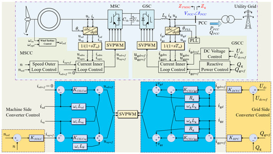
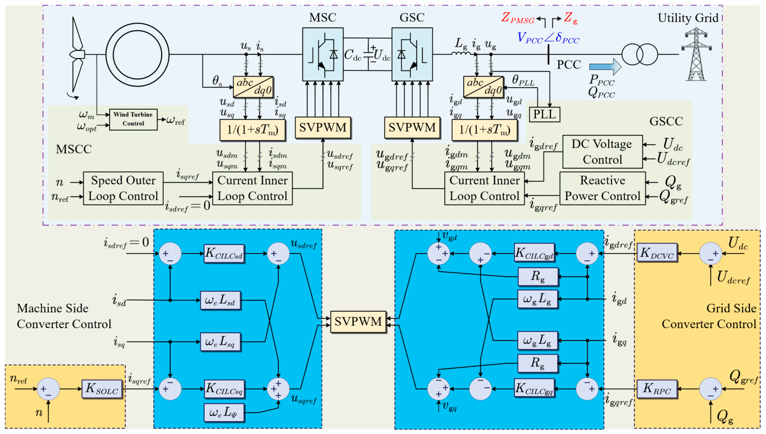
Figure 1 illustrates the typical structure and control strategy of a permanent magnet synchronous generator (PMSG) integrated into the power grid. The system comprises a wind turbine and its control system, a PMSG, a full-power converter system, and a generator-side filter inductor. The full-power converter and its control system are divided into three components: the Machine-Side Converter (MSC) with its control system, a DC capacitor for voltage stabilization, and the Grid-Side Converter (GSC) with its control system. Both the MSC and GSC employ $dq$-decoupling control strategies to simplify the control of alternating current machines. The MSC regulates the generator’s output power according to the optimal speed reference, while the GSC maintains DC-link voltage stability and adjusts the wind turbine’s reactive power output to support voltage regulation.

Figure 1. A schematic diagram of the grid connection structure and control method of PMSG.

The equivalent model of the utility grid employs a Thevenin grid voltage source $V_{PCC}$ and impedance $Z_g$. In this study, a standard 2-MW PMSG model, configured according to the motor convention, is utilized for training data acquisition and frequency-domain simulation. Controller limiters are not modeled in this analysis. This exclusion does not impact the admittance modeling of the PMSG, as admittance modeling is a small-signal analysis that describes a linearized steady-state model around a specific operating point.

2.2. AM of PMSG

The dynamic behavior of PMSG can be characterized by an AM. The AM can be established in either the sequence domain or the $dq$ reference frame. In this paper, the AM is developed in the $dq$ frame and denoted ${\mathbf{Y}}_{\mathrm{dq}}$. In general, the AM relates the inverter output voltage $v_{\mathrm{pcc}}=V_{\mathrm{d}}+j{V}_{\mathrm{q}}$ to the point-of-common-coupling (PCC) current $i_{\mathrm{pcc}}=I_{\mathrm{d}}+j{I}_{\mathrm{q}}$ as follows:

$$\left[\begin{array}{c}{I}_{\mathrm{d}}\\ I_{\mathrm{q}}\end{array}\right]=\underset{{\mathbf{Y}}_{\mathrm{dq}}}{\underbrace{\left[\begin{array}{cc}{Y}_{\mathrm{dd}}& Y_{\mathrm{dq}}\\ Y_{\mathrm{qd}}& Y_{\mathrm{qq}}\end{array}\right]}}\times \left[\begin{array}{c}{V}_{\mathrm{d}}\\ V_{\mathrm{q}}\end{array}\right],$$

(1)

Here, $Y_{\mathrm{dd}}$ and $Y_{\mathrm{qq}}$ denote the diagonal admittances of the AM along the d and q axes, respectively. The terms $Y_{\mathrm{dq}}$ and $Y_{\mathrm{qd}}$ correspond to the IM’s off-diagonal elements, which characterize the coupling between the d and q axes.

The matrix ${\mathit{Y}}_{\mathrm{dq}}$ may be determined either analytically or through measurement. Although the analytical method provides an accurate characterization of the AM, it is generally impractical for engineering applications because of commercial confidentiality constraints. Therefore, ${\mathit{Y}}_{\mathrm{dq}}$ is typically measured using identification techniques, where perturbations such as single- or multi-tone frequency scanning or pseudo-random binary sequence (PRBS) methods are applied to the d and q axes. To obtain linearly independent vectors for solving the AM, two independent measurement sets, $(I_{\mathrm{d}1},I_{\mathrm{q}1},V_{\mathrm{d}1},V_{\mathrm{q}1})$ and $(I_{\mathrm{d}2},I_{\mathrm{q}2},V_{\mathrm{d}2},V_{\mathrm{q}2})$, are required, as shown below:

$$\left[\begin{array}{cc}{Y}_{\mathrm{dd}}& Y_{\mathrm{dq}}\\ Y_{\mathrm{qd}}& Y_{\mathrm{qq}}\end{array}\right]=\left[\begin{array}{cc}{I}_{\mathrm{d}1}& I_{\mathrm{d}2}\\ I_{\mathrm{q}1}& I_{\mathrm{q}2}\end{array}\right]\times {\left[\begin{array}{cc}{V}_{\mathrm{d}1}& V_{\mathrm{d}2}\\ V_{\mathrm{q}1}& V_{\mathrm{q}2}\end{array}\right]}^{-1}.$$

(2)

However, the measured ${\mathit{Y}}_{\mathrm{dq}}$ in (2) is only valid for the corresponding OP. Once the OP of the PMSG changes, ${\mathit{Y}}_{\mathrm{dq}}$ needs to be measured again.

OP variations mainly arise from two causes:

• External events that modify the equivalent grid admittance—such as faults, load connection/disconnection, and generator start-up/shutdown.
• Deliberate set-point adjustments of the PMSG—for example, injecting reactive power to support the grid voltage.

Both categories lead to OP shifts and fluctuations. The OP dependence of the AM introduces substantial challenges for stability assessment under varying OPs. Consequently, an admittance prediction algorithm is needed to estimate the corresponding ${\mathit{Y}}_{\mathrm{dq}}$ at a new OP without repeating the measurement/identification procedure.

2.3. Impacts of the Variable OPs on PMSG

In the investigated PMSG system, the Grid-Side Converter operates in GFL mode. To evaluate the impact of OP variations on the AM of the PMSG, an analytical $dq$-domain AM is employed. The system parameters are summarized in Table 2.

Table 2. Parameters used for PMSG.

Parameter	Symbol	Value	Unit
Grid voltage (RMS, L-L)	$V_g$	690	V
Grid frequency	$f_g$	50	Hz
Rated power	$S_n$	2	MVA
Pole pairs	$N_p$	48	/
Rotor flux linkage	${\mathsf{\Psi }}_{\mathrm{f}}$	3.88889	Wb
d-axis stator inductance	$L_{\mathrm{sd}}$	1.8 × 10−3	H
q-axis stator inductance	$L_{\mathrm{sq}}$	1.8 × 10−3	H
Stator resistance	$R_{\mathrm{s}}$	2.6 × 10−3	$\mathsf{\Omega }$
Pitch angle	$\beta$	0	Deg
Moment of inertia	$J$	35,000	$\mathrm{kg}\cdot {\mathrm{m}}^2$
Mechanical damping coefficient	$D_{\mathrm{m}}$	7.8 × 10−2	N·m·s/rad
Wind turbine rotor radius	$R_{\mathrm{t}}$	36.6	m
Air density	$\rho$	1.12	$\mathrm{kg}\cdot {\mathrm{m}}^3$
Rated wind speed	vw	12	m/s
DC voltage	$V_{\mathrm{dc}}$	1150	V
DC-link Capacitor	$C_{\mathrm{dc}}$	1 × 10−3	F
Grid-side filter inductance	$L_f$	7 × 10−3	H
Grid-side filter resistor	$R_f$	5 × 10−2	$\mathsf{\Omega }$

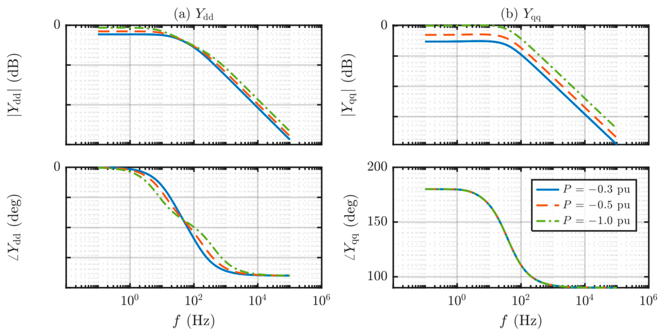
Since the phase-locked loop (PLL) enforces $V_{\mathrm{q}}=0$ during synchronization with the grid voltage, three operating points are considered by varying only the active power output $P$ (−0.3, −0.5, and −1 p.u.), while maintaining the reactive power $Q=0$ p.u. and the grid voltage magnitude $V$ at 1 p.u. For each OP, the diagonal admittance elements $Y_{\mathrm{dd}}$ and $Y_{\mathrm{qq}}$ are extracted from the analytical dq-domain AM.

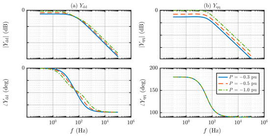
Figure 2 illustrates the influence of OP variations on the magnitude and phase characteristics of $Y_{\mathrm{dd}}$ and $Y_{\mathrm{qq}}$. As shown in Figure 2a, under the condition $Q=0$, $V=1$, and $\xi =0$, the $Y_{\mathrm{dd}}$ component exhibits significant sensitivity to the operating point. As |P| increases, the magnitude $\left|Y_{\mathrm{dd}}\right|$ rises noticeably in the mid-to-high frequency range, while the phase roll-off region of $\angle Y_{\mathrm{dd}}$ shifts accordingly, indicating that the effective dynamic behavior of the system varies with the operating point.

Figure 2. Bode plots of the AM of the PMSG considering variable OPs: (a) $Y_{\mathrm{dd}}$, and (b) $Y_{\mathrm{qq}}$.

In contrast, as depicted in Figure 2b, although the magnitude of $Y_{\mathrm{qq}}$ shows a certain offset across different operating points, its overall frequency-dependent trend remains consistent. Moreover, the phase responses of $Y_{\mathrm{qq}}$ under the three operating conditions nearly overlap, demonstrating that the phase characteristic of $Y_{\mathrm{qq}}$ is largely insensitive to variations in the operating point.

3. Equivalent-Circuit Transformation Method Based on VF

This section first outlines the principle of VF as a modeling tool, and then elaborates on the methods for equivalent-circuit transformation and component parameter calculation based on VF.

3.1. Principle of VF Algorithm

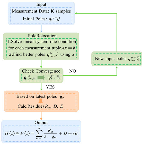
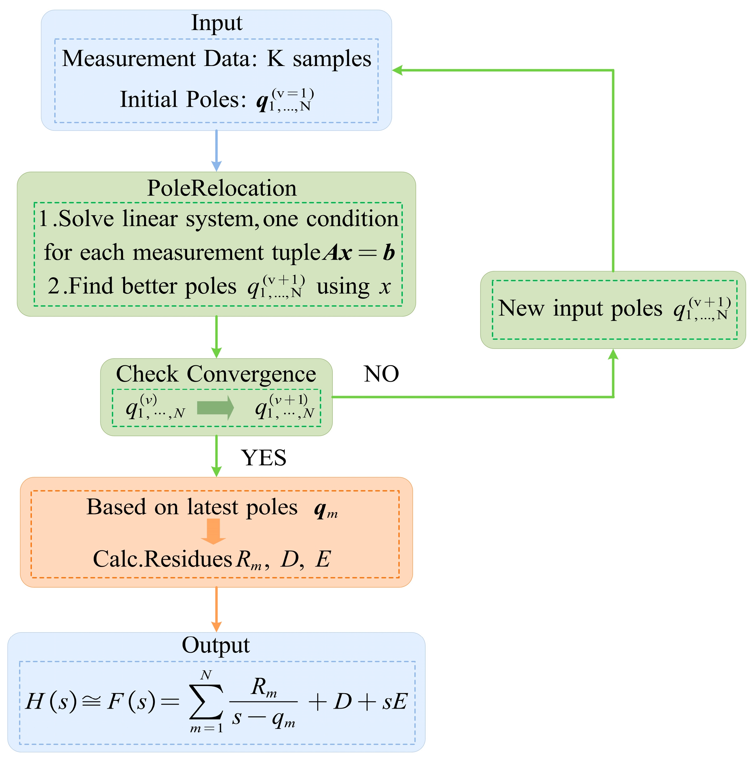
The VF algorithm developed in [31,32,33] is widely used to obtain a rational approximation of a black-box model from frequency response measurements $H\left(s\right)$. The flow chart describing the working principle of the VF algorithm is shown in Figure 3. VF seeks a rational fitting function $F\left(s\right)$ by iteratively minimizing the least-squares objective in Equation (3):

$$E_2\approx \min {\displaystyle \sum _{k=1}^K\parallel H\left(s_k\right)}-F(s_k){\parallel }^2,$$

(3)

Figure 3. Flow chart of VF algorithm.

The fitting function $F\left(s\right)$ with partial fraction basis is assumed to be in the form of Equation (4):

$$F\left(s\right)={\displaystyle \sum _{m=1}^N\frac{R_m}{s-a_m}}+D+sE,$$

(4)

where $q_m$ are the poles and $R_m$, $D$, $E$ are unknown variables.

For the frequency-domain AM, the frequency response measurements of the PMSG are collected at ${\left\{s_k\right\}}_{k=1}^K$, where $K$ represents the number of measurements and ${\left\{H\right(s_k)\}}_{k=1}^K$ denotes the frequency response, specifically the frequency-dependent PMSG admittance at each $s_k$. Because the AM is influenced by the control structure and design parameters, resonance peaks may occur. To address potential ill-conditioning in the fitting process, the initial poles are chosen as complex values, denoted by $q_{1\dots N}^{v=1}$, where $N$ is the number of poles (i.e., the selected system order), and $q^{v=1}$ refers to the pole set at the first iteration.

Because the initial poles are chosen arbitrarily, VF performs pole relocation, in which the poles are updated iteratively until convergence, i.e., $q_{1\dots N}^v\approx q_{1\dots N}^{v+1}$. This pole relocation step is achieved by minimizing the least squares problem $E_2$. Considering $F\left(s\right)$ is in the form of ${\displaystyle \frac{N\left(s\right)}{D\left(s\right)}}$ where $N\left(\begin{array}{c}s\end{array}\right)$ and $D\left(s\right)$ are the numerator and denominator of the fitting function $F\left(s\right)$ defined as in Equation (6), the error $E_2$ can be expressed as Equation (5):

$$\min {\displaystyle \sum _{k=1}^K\frac{1}{\left|D^v\right(s_k){|}^2}{\left|N^v\left(s_k\right)-D^v\left(s_k\right)H\left(s_k\right)\right|}^2},$$

(5)

$$F(s)={\displaystyle \frac{{\displaystyle \sum _{m=1}^N\frac{r_m}{s-q_m^v}}+d+se}{d_0+{\displaystyle \sum _{m=1}^N\frac{w_m}{s-q_m^v}}}},$$

(6)

The minimization problem $E_2$ in Equation (3) is nonlinear. Hence, following the Sanathanam–Koerner iteration technique, at each iteration $v$, the problem is linearized at each iteration $v$ [34] and cast into the form $Ax=b$, where

$$\underset{b}{\underbrace{H\left(s\right)}}=\underset{A}{\underbrace{\left[{\displaystyle \frac{1}{s-q_0}},\cdots ,{\displaystyle \frac{1}{s-q_n}},1,s,\cdots ,{\displaystyle \frac{H\left(s\right)}{s-q_0}},\cdots ,{\displaystyle \frac{H\left(s\right)}{s-q_N}}\right]}}\underset{x}{\underbrace{{\left[r_0,\dots ,r_N,d,e,w_0,\dots ,w_N\right]}^T}}.$$

(7)

Given the pole set from the previous iteration $q^{v-1}$ and the measurement data $H\left(s\right)$, the unknown vector $\mathit{x}$ is first computed. The poles $q^{v+1}$ are then updated from the identified $\mathit{x}$. This iterative process continues until convergence. Upon convergence, the final residues obtained from the residue-calculation step are used to construct a transfer function that emulates the frequency-dependent PMSG admittance.

In standard VF, choosing $d_0=1$ results in a biased approximation. To address this limitation, VF is modified by treating $d_0$ as an additional free variable, resulting in the augmented unknown vector described in Equation (8). An additional constraint ensures that $d_0$ remains non-zero, allowing it to participate in the pole relocation step. This modification is termed relaxed vector fitting (RVF):

$$x={[r_0,\dots ,r_N,d,e,w_0,\dots ,w_N,d_0]}^T.$$

(8)

3.2. Equivalent-Circuit Conversion Method

Once the rational-function parameters $R_m$, $q_m$, $D$, and $E$ are obtained via the vector fitting algorithm, the function is decomposed into three parts—(i) the constant and proportional terms, (ii) the contributions from real poles and their residues, and (iii) the contributions from complex-conjugate pole pairs and their residues. This decomposition enables computation of the parameters of the corresponding equivalent circuit, namely $R$, $L$, $\mathrm{C}$, and g_m. As described in [35], the equivalent-circuit model is constructed from:

• The subcircuit associated with the $\mathrm{D}+\mathrm{sE}$ term;
• The subcircuit corresponding to the real-pole part, ${\displaystyle \sum _{m=1}^N}{\displaystyle \frac{R_{m,i}}{s-q_{m,i}}}$;
• The subcircuit corresponding to the complex-conjugate pairs, ${\displaystyle \sum _{m=1}^N}\left({\displaystyle \frac{R_{m,i}}{s-q_{m,i}}}+{\displaystyle \frac{R_{m,i}^{*}}{s-q_{m,i}^{*}}}\right)$, where $\mathrm{s}$ is the Laplace variable and ${(\cdot )}^{*}$ denotes complex conjugation.

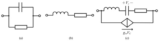
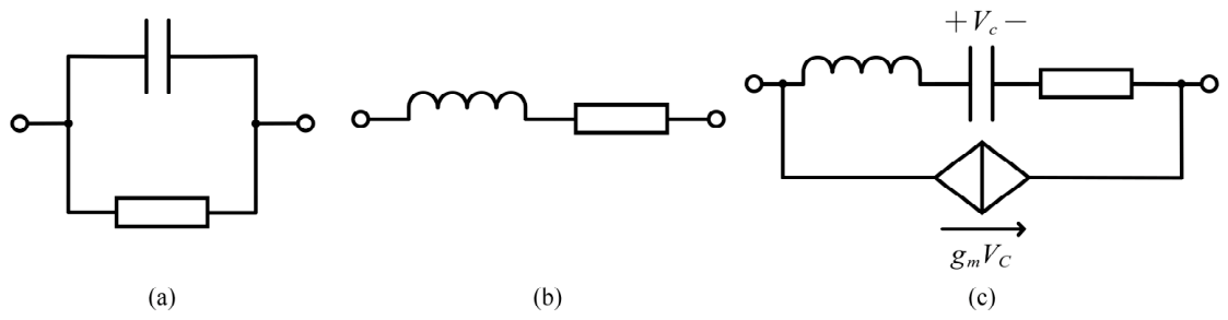
Specifically, these three components are represented by equivalent subcircuits in the admittance form $Y\left(s\right)$. As shown in Figure 4: (a) an RC parallel network represents the constant and proportional terms; (b) a series RL branch represents the real-pole/residue contribution; and (c) a series RLC branch combined with a voltage-controlled current source (VCCS) represents the contribution of complex-conjugate pole pairs and their residues.

Figure 4. Equivalent subcircuit schematics: (a) RC parallel branch for the constant and proportional terms; (b) series RL branch for a real-pole term; (c) series RLC branch with a VCCS for a complex-conjugate pole pair.

(a) Constant and proportional term $D+sE$:

The constant–proportional part is realized by an $\mathrm{RC}$ parallel network.

The target admittance is $H_{\mathrm{target}}\left(s\right)=D_i+s{E}_i$, while the RC parallel network admittance is $Y_{RC}(s)={\displaystyle \frac{1}{R}}+sC$.

Choosing $R={\displaystyle \frac{1}{D_i}}$ and $C=E_i$ gives an exact match, $Y_{RC}\left(s\right)=H_{\mathrm{target}}\left(s\right)$.

(b) Real pole with residue ${\displaystyle \sum _{m=1}^N}{\displaystyle \frac{R_m}{s-q_m}}$:

Each real-pole term is synthesized by a series $\mathrm{RL}$ branch.

For a single term, $H_{\mathrm{target}}(s)={\displaystyle \frac{R_{m,i}}{s-q_{m,i}}}$. The series $\mathrm{RL}$ branch has admittance $Y_{RL}(s)={\displaystyle \frac{\frac{1}{L}}{s+\frac{R}{L}}}$.

Setting $L={\displaystyle \frac{1}{R_{m,i}}}$ and $R={\displaystyle \frac{-q_{m,i}}{R_{m,i}}}$ yields $Y_{RL}(s)={\displaystyle \frac{R_{m,i}}{s-q_{m,i}}}$.

(c) Complex-conjugate pole pair ${\displaystyle \sum _{m=1}^N}{\displaystyle \frac{R_m}{s-q_m}}+{\displaystyle \frac{R_m^{*}}{s-q_m^{*}}}$:

In vector fitting, complex poles $q_m={q^{\prime }}_m+j{q^{″}}_m$, and residues $R_m={R^{\prime }}_m+j{R^{″}}_m$ appear as conjugate pairs $(q_m,q_m^{*})$ and $(R_m,R_m^{*})$. Their combined contribution is

$$H_{\mathrm{target}}(s)={\displaystyle \frac{R_m}{s-q_m}}+{\displaystyle \frac{R_m^{*}}{s-q_m^{*}}}={\displaystyle \frac{2{R^{\prime }}_{m}s-2\left({R^{\prime }}_m{q^{\prime }}_m+{R^{″}}_m{q^{″}}_m\right)}{s^2-2{q^{\prime }}_{m}s+|q_m{|}^2}}$$

which is realized by a series RLC branch augmented with a voltage-controlled current source (VCCS) referenced to the capacitor voltage. The augmented branch admittance is

$$Y_{RLC,I}(s)={\displaystyle \frac{\left(\frac{1}{L}\right)s+b}{s^2+\left(\frac{R}{L}\right)s+\frac{1}{LC}}}$$

Choosing $L={\displaystyle \frac{1}{2{R^{\prime }}_m}},\hspace{1em}R={\displaystyle \frac{-{q^{\prime }}_m}{{R^{\prime }}_m}},\hspace{1em}C={\displaystyle \frac{2{R^{\prime }}_m}{|q_m{|}^2}},\hspace{1em}b=-2({R^{\prime }}_m{q^{\prime }}_m+{R^{″}}_m{q^{″}}_m);$ gives $Y_{RLC,I}\left(s\right)=H_{\mathrm{target}}\left(s\right)$. The VCCS transconductance can be written as $g_n\triangleq bLC={\displaystyle \frac{b}{|q_m{|}^2}},$

here $|q_m{|}^2={\left({q^{\prime }}_m\right)}^2+{\left({q^{″}}_m\right)}^2$.

It should be noted that the synthesized circuit is a behavioral equivalent representation of the fitted admittance function rather than a literal hardware circuit inside the PMSG system. Nevertheless, these parameters retain physical interpretability at the terminal-behavior level. For example, equivalent resistive terms are associated with damping or negative-damping characteristics, inductive and capacitive terms describe frequency-dependent phase and energy exchange behavior, and controlled source terms represent coupling effects introduced by converter control loops and $dq$-axis interactions.

4. Proposed SVM-Based Method for Predicting Equivalent-Circuit Element Parameters

The following subsections provide an overview of the SVM as a modeling tool, followed by a detailed description of the proposed SVM-based method for predicting equivalent-circuit element parameters, and then inversely derive each fraction of the rational function model from the equivalent-circuit element parameters according to the formulas in Section 3.2, which are combined to form the admittance transfer function under new OPs.

4.1. SVM as a Modeling Tool

Support vector machines (SVMs) are supervised learning algorithms commonly used for classification and regression. They demonstrate particular effectiveness with complex datasets that exhibit nonlinear feature relationships. SVMs are recognized for their ability to manage high-dimensional data and their robustness to overfitting. As a result, SVMs have been used across diverse domains, including image recognition, text classification, and bioinformatics [36,37,38].

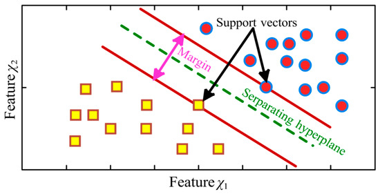
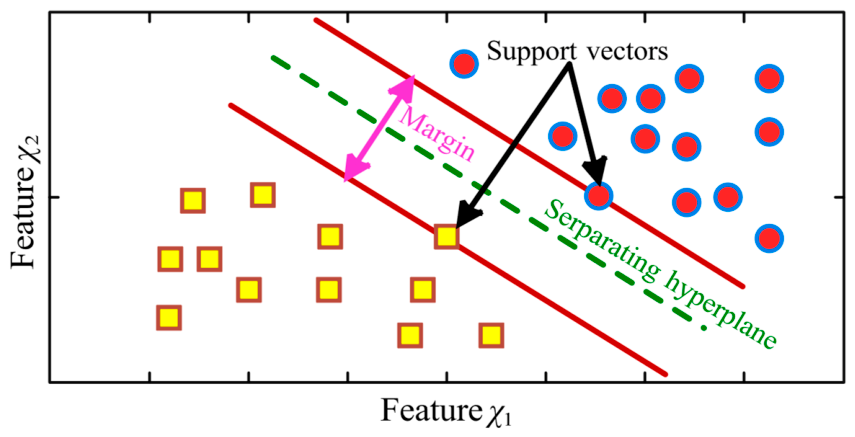
For linearly separable problems, the fundamental principle of SVM operation is depicted in Figure 5. The SVM identifies an optimal separating hyperplane between classes by maximizing the margin, which is the distance from the hyperplane to the nearest samples of each class. This maximization is enforced by the margin (also called the RVF constraint), which ensures that all samples lie on the correct side of the margin, thereby increasing separation and robustness. The samples closest to the hyperplane, known as support vectors, primarily define the decision boundary.

Figure 5. SVM classification for a linearly separable dataset.

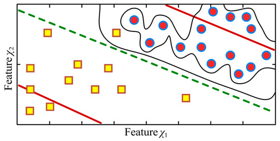
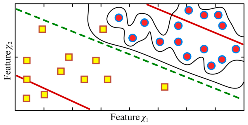
For linearly non-separable problems commonly encountered in practice, SVMs employ the soft-margin formulation and kernel methods. The soft margin permits limited violations of separability to balance margin maximization with empirical error minimization. Kernel methods, implemented via kernel functions as depicted in Figure 6, map the input data into a (possibly higher-dimensional) feature space, enabling the construction of nonlinear decision boundaries. The kernel-based SVM formulation adopted in this paper for predicting equivalent-circuit element parameters is summarized below.

Figure 6. SVM classification for a linearly non-separable dataset.

Given a training dataset $X_i$ (where $i=1, 2, 3, \dots ,N$), the kernelized hyperplane for linearly non-separable data using a kernel function $K(X,X_i)$ is expressed as

$$Y={\beta }_0+{\displaystyle \sum _{i=1}^N{\alpha }_i{y}_{i}K(X,X_i)},$$

(9)

where $Y$ denotes the nonlinear decision function that represents the predicted output for a new data point. ${\beta }_0$ is the bias term, $N$ is the number of training samples, ${\alpha }_i$ are the Lagrange multipliers associated with the training samples, and $y_i$ denotes the target output value for the $i^{th}$ sample in regression or the class label in classification. For the regression task addressed in this study, which aims to predict the equivalent-circuit element parameter, $y_i$ corresponds to the PMSG output admittance in the $dq$ reference frame used for training. $K(X,X_i)$ is the kernel function evaluated on $X$ and $X_i$, characterizing the similarity between the two samples.

During training, the objective is to determine the Lagrange multipliers ${\alpha }_i$ that maximize the margin in the induced feature space while considering pairwise relationships among training samples. This objective is achieved by maximizing the following [39]:

$${\max }_{\alpha }{\displaystyle {\displaystyle \sum _{i=1}^N}{\alpha }_i}-{\displaystyle \frac{1}{2}}{\displaystyle {\displaystyle \sum _{i=1}^N}{\displaystyle \sum _{j=1}^N{\alpha }_i{\alpha }_j{y}_i{y}_{j}K(X_i,X_j)}},$$

(10)

subject to

$$\left\{\begin{array}{l}0\le {\alpha }_i\le C\hfill \\ {\displaystyle \sum _{i=1}^N{\alpha }_i{y}_i}=0\hfill \end{array}\right.$$

(11)

for all training samples, where $C$ is the regularization parameter.

The kernel function $K(X_i,X_j)$ evaluates the similarity between samples $X_i$ and $X_j$ in the original feature space. Although the data may not be linearly separable in the input space, kernel mapping can render them separable in a higher-dimensional space, thereby enabling more flexible decision boundaries. The kernel selection depends on the data characteristics and the target task; commonly used kernels include linear, polynomial, and Gaussian radial basis function (RBF) kernels. Recent studies have also shown that kernel adjustment in SVMs can improve their ability to handle complex and imbalanced datasets by reshaping nonlinear decision boundaries, further highlighting the importance of kernel selection and parameter tuning in SVM-based learning [40]. In this paper, the RBF kernel is adopted due to its prevalence in the SVM literature and its ability to capture complex nonlinear decision boundaries [41]. With $\sigma$ denoting the kernel width, the RBF kernel is defined as

$$K(X_i,X_j)=\exp \left(-{\displaystyle \frac{\parallel X_i-X_j{\parallel }^2}{2{\sigma }^2}}\right).$$

(12)

4.2. SVM for Predicting Component Parameters of Equivalent Circuits

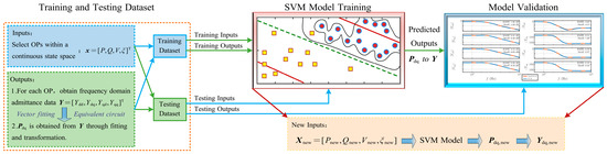
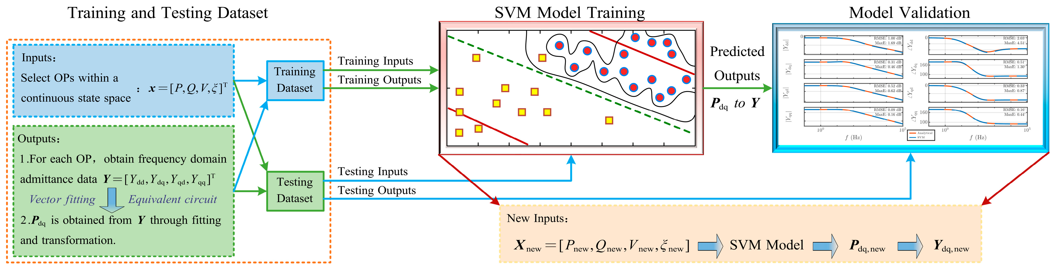
Figure 7 illustrates the methodological framework of the SVM-based prediction approach for equivalent-circuit element parameters of the PMSG in the synchronous rotating $dq$ reference frame. Table 3 shows the explanation of the symbols used in this section.

Figure 7. The methodological framework of the SVM-based prediction approach for equivalent-circuit element parameters.

Table 3. Organization of admittance channels, equivalent-circuit parameters, and SVR models.

Symbol	Meaning	Dimension
$N_{\mathrm{op}}$	Number of operating-point samples	scalar
$K$	Number of frequency samples	scalar
$x^{\left(n\right)}$	OP feature vector	$4\times 1$
$Y_{dq}^{\left(n\right)}$(s)	dq-frame admittance matrix	$2\times 2$
$Y_{ij}^{\left(n\right)}$(s)	One scalar admittance channel	scalar transfer function
${\mathit{\theta }}_{ij}^{\left(n\right)}$	Parameter vector of $Y_{ij}$	$n_{p,ij}\times 1$
${\theta }_{ij,r}^{\left(n\right)}$	The $r$-th branch parameter of $Y_{ij}$	scalar
$f_{ij,r}$	SVR for ${\theta }_{ij,r}$	one scalar-output SVR
$\mathcal{F}$	Complete SVR model set	${\displaystyle \sum _{i,j}{n}_{p,ij}}$ SVRs.

For clarity, let $N_{\mathrm{op}}$ denote the number of operating-point samples and $K$ denote the number of sampled frequency points. For the $n$-th operating point, the input feature vector is defined as $x^{\left(n\right)}={[P^{\left(n\right)},Q^{\left(n\right)},V^{\left(n\right)},{\xi }^{\left(n\right)}]}^T$. The corresponding admittance model in the synchronous reference frame is expressed as a $2\times 2$ matrix, including four scalar admittance channels, i.e., $Y_{dd}^{\left(n\right)}(s)$, $Y_{dq}^{\left(n\right)}(s)$, $Y_{qd}^{\left(n\right)}(s)$, and $Y_{qq}^{\left(n\right)}(s)$. Each admittance channel is independently fitted by VF and then transformed into an equivalent-circuit representation. And it can be converted into a parameter matrix ${\mathit{P}}_{\mathrm{dq}}$, defined as

$${\mathit{P}}_{\mathrm{dq}}=\left[\begin{array}{cc}{\mathit{P}}_{\mathrm{dd}}& {\mathit{P}}_{\mathrm{dq}}\\ {\mathit{P}}_{\mathrm{qd}}& {\mathit{P}}_{\mathrm{qq}}\end{array}\right].$$

(13)

The resulting equivalent-circuit parameter vector of $Y_{ij}^{\left(n\right)}(s)$ is denoted as ${\mathit{\theta }}_{ij}^{\left(n\right)}={[{\theta }_{ij,1}^{\left(n\right)},{\theta }_{ij,2}^{\left(n\right)},\dots ,{\theta }_{\mathrm{ij},n_{p,\mathrm{ij}}}^{\left(n\right)}]}^T,\hspace{1em}i,j\in \{d,q\},$ where $n_{p,ij}$ is determined by the synthesized equivalent-circuit topology of the corresponding admittance channel. The symbols $R$, $L$, $C$, and $g_m$ represent categories of equivalent-circuit parameters rather than four fixed output variables.

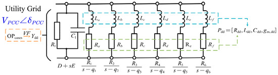
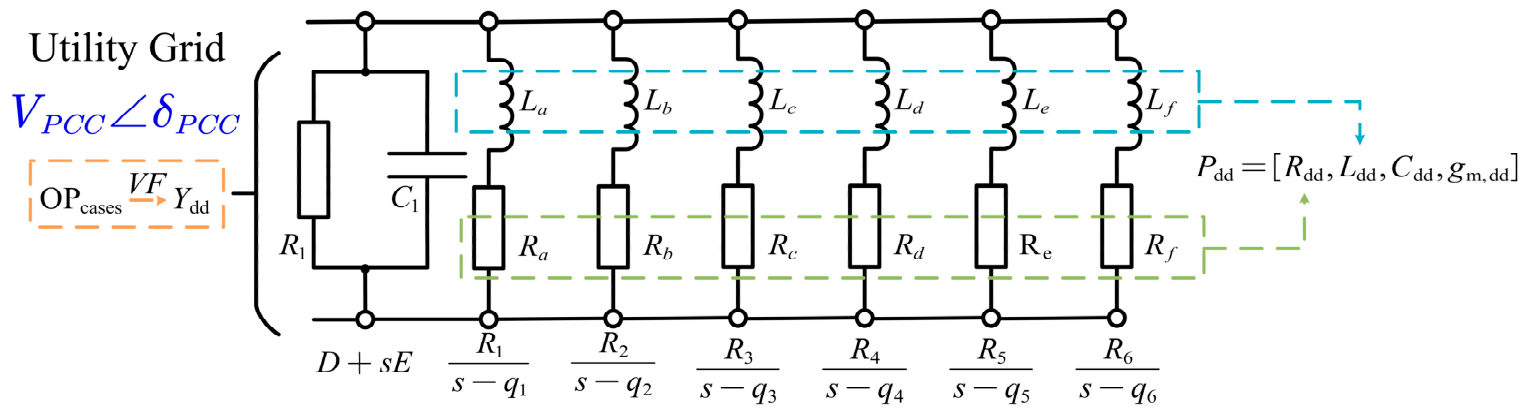
In the present PMSG case, the synthesized topology shown in Section 5.2 consists of one RC parallel branch and six RL series branches for the illustrated admittance channel. Therefore, the corresponding parameter vector can be arranged as

$${\mathit{\theta }}_{dd}^{\left(n\right)}={[R_{0,dd}^{\left(n\right)},C_{0,dd}^{\left(n\right)},R_{a,dd}^{\left(n\right)},L_{a,dd}^{\left(n\right)},\dots ,R_{f,dd}^{\left(n\right)},L_{f,dd}^{\left(n\right)}]}^T.$$

Other admittance channels are processed in the same manner, with their parameter vectors organized according to their own synthesized circuit topologies.

Under the black-box scenario, the input and output vector datasets required for model training and testing can be obtained through disturbance injection and response measurement. In the white-box scenario, the aforementioned input and output vectors can be obtained directly via analytical derivation.

The frequency-domain dynamic behavior of the PMSG in the power grid, characterized by the AM, is affected by multiple factors, including grid admittance, load variations, operating-point fluctuations, the control algorithm, and internal interactions within cascaded control loops. The coupling of these factors complicates the accurate modeling of PMSG. Accordingly, the SVM-based method proposed in this paper formulates parameter prediction for equivalent-circuit elements as a nonlinear, non-separable problem and employs the radial basis function (RBF) kernel to address it.

Since this article is a regression prediction problem, the support vector regression model in the support vector machine is used. The SVR model is trained in a parameter-wise manner. For the $r$-th equivalent-circuit parameter of $Y_{ij}$, its values over all operating points form a scalar target vector: ${\mathit{\theta }}_{ij,r}={[{\theta }_{ij,r}^{\left(1\right)},{\theta }_{ij,r}^{\left(2\right)},\dots ,{\theta }_{ij,r}^{{(N}_{\mathrm{op}})}]}^T.$

An independent scalar SVR model is then trained as ${\widehat{\theta }}_{ij,r}=f_{ij,r}(x),\hspace{1em}r=1,\dots ,n_{p,ij}.$

Hence, the proposed implementation is an ensemble of independent single-output SVR models.

The workflow of the proposed SVM-based AM prediction approach is detailed in the following steps:

• Dataset Preparation
  • Construction of Representative OP Subset: $N$ groups of typical operating points covering the full operating range are selected to establish the basic sample set for model training and testing.
  • Construction of Model Input Feature Set: The input feature vector for a single operating point is defined as $\mathit{x}={[P,Q,V,\xi ]}^{\mathrm{T}}$, where $P$, $Q$, and $V$ denote the active power, reactive power, and grid voltage amplitude of the corresponding operating point, all expressed in per-unit (p.u.) values; $\xi$ denotes the phase angle of the grid voltage with the unit of radians (rad). By stacking the feature vectors of $N$ operating points row-wise, the input dataset matrix for the SVM model is constructed as $\mathit{X}\in {ℝ}^{N\times 4}$, where each row corresponds to the complete features of one operating point, and each column corresponds to one feature dimension.
  • For each operating point, the four admittance channels $Y_{\mathrm{dd}}$, $Y_{\mathrm{dq}}$, $Y_{\mathrm{qd}}$, and $Y_{\mathrm{qq}}$ are extracted from the $dq$-frame admittance matrix. Each channel is independently fitted by VF and converted into its corresponding equivalent-circuit topology.
  • According to the equivalent-circuit conversion formulas in Section 3.2, the branch parameters of each synthesized topology are calculated. The extracted parameters may include resistances, inductances, capacitances, and VCCS transconductances, depending on whether the corresponding topology contains RC, RL, or RLC–VCCS subcircuits.
  • For each admittance channel $Y_{ij}$ and each equivalent-circuit parameter ${\theta }_{ij,r}$, the parameter values obtained under all operating points are collected as a scalar target vector. One independent SVR model is trained for this target vector. This parameter-wise construction avoids ambiguity in output dimensions and allows each branch parameter to be normalized and predicted separately.
• SVM Model Training: Construction and Training of SVM Model: Based on the input feature matrix $\mathit{X}\in {ℝ}^{N\times 4}$ and the output target matrix ${\mathit{P}}_{\mathrm{dq}}$ constructed in the dataset preparation section, the dataset is divided into the training set and validation set, to establish the nonlinear mapping relationship between OPs of PMSG and the equivalent-circuit element parameters in the $dq$ reference frame.
• SVM Model Validation: Validate prediction accuracy using an independent test set that does not overlap with the training set.
• AM Prediction for New Inputs: Based on the well-trained SVR model, for the input feature vector of any new operating condition ${\mathit{X}}_{\mathrm{new}}=[P_{\mathrm{new}},Q_{\mathrm{new}},V_{\mathrm{new}},{\xi }_{\mathrm{new}}]$, the corresponding equivalent-circuit element parameter matrix ${\mathit{P}}_{\mathrm{dq},\mathrm{new}}$ can be directly predicted, and then the $dq$-frame AM ${\mathit{Y}}_{\mathrm{dq},\mathrm{new}}$ in the full frequency range can be analytically generated.

With the proposed method, it is unnecessary to re-derive the frequency-domain analytical model of the PMSG for new OPs, nor to repeat the frequency-domain perturbation measurement experiments. The frequency-domain dynamic characteristics of the PMSG under variable operating conditions can be obtained quickly and accurately.

5. Performance Evaluation

5.1. Training and Testing Dataset

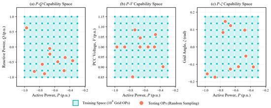
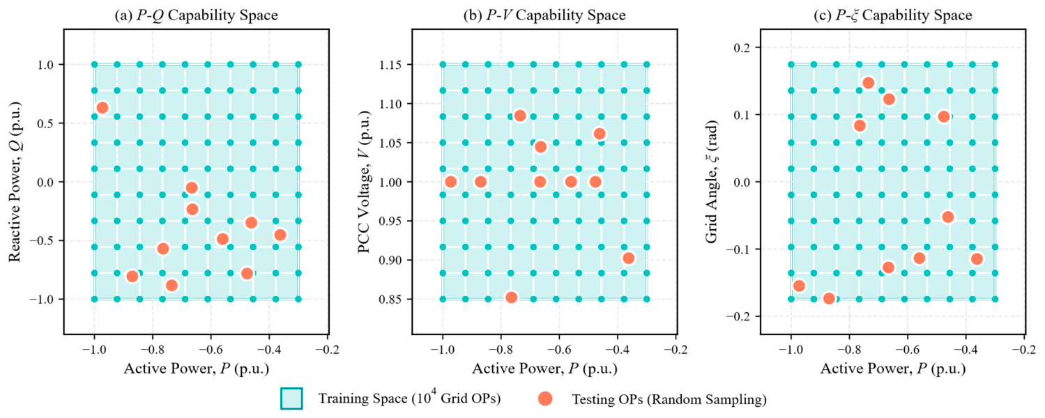
Figure 8 illustrates the generation logic and coverage of the training and testing datasets used in this study. To verify the generalization capability of the proposed SVM model, a grid-search multidimensional sampling strategy is adopted. This strategy comprehensively covers various steady-state OPs of PMSG.

Figure 8. Training and testing datasets.

The characteristic parameters of the OPs in the training dataset are defined within a continuous state space $\mathit{x}={[P,Q,V,\xi ]}^{\mathrm{T}}$, and the specific rules for linear uniform discretization are as follows:

• Active Power ($P$): 10 discrete points are uniformly distributed within the range of $[-1,-0.3]$ p.u. (following the motor convention, negative values denote the generating state of the PMSG), strictly covering the medium- and full-load rated operating conditions with fine granularity.
• Reactive Power ($Q$): 10 discrete points are uniformly selected within $[-1,1]$ p.u. This full range accurately accounts for the inductive and capacitive reactive power support capabilities required by grid standards.
• PCC Voltage Magnitude ($V$): 10 equally spaced points are configured within the range of $[0.85,1.15]$ p.u. This ultra-wide continuous operating range exceeds conventional industry-standard limits (e.g., the $[0.96,1.1]$ p.u. limit specified in IEEE 1547 [42] and AS/NZS 4777 [43,44]), thereby ensuring adequate representation of extreme operating scenarios.
• Grid Voltage Phase Angle ($\xi$): 10 discrete points are uniformly extracted within $[-\mathrm{pi}/18,\mathrm{pi}/18]$ rad (i.e., $-10°$ to $+{10}^{°}$) to simulate angle deviations induced by power flow shifts and grid disturbances.

By traversing wide ranges of $V$ and $\xi$, this multidimensional sampling strategy seamlessly integrates ideal strong grid conditions with non-ideal weak grid scenarios—selecting a critically weak grid with a short-circuit ratio (SCR) of 2, which typically provokes severe fluctuations in both the PCC voltage magnitude and phase angle.

The admittance data required for training and testing can generally be obtained via frequency-scanning measurements using electromagnetic transient (EMT) models, or through direct analytical computation based on detailed state-space models. To ensure mechanistic rigor and sampling efficiency, this study uses the detailed analytical model of the PMSG derived in Section 2 to generate the dataset. The frequency sampling range for the AM is configured as $[1\times {10}^{-1},1\times {10}^{-5}]$ Hz, within which 200 sampling frequencies are extracted using a logarithmic distribution.

For each OP, the dataset maps the system-side operating input features $\mathit{x}={[P,Q,V,\xi ]}^{\mathrm{T}}$ to the corresponding $2\times 2$ equivalent-circuit block-parameter matrix ${\mathit{P}}_{\mathrm{dq}}$ as the output target. The elements of ${\mathit{P}}_{\mathrm{dq}}$ are fitted and transformed from the source frequency-domain admittance data $\mathit{Y}={[Y_{\mathrm{dd}},Y_{\mathrm{dq}},Y_{\mathrm{qd}},Y_{\mathrm{qq}}]}^{\mathrm{T}}$. In summary, the full-range operating input limits of the PMSG strictly satisfy—and even exceed—the steady-state requirements stipulated in GB/T 19963.1-2021 [45] and IEEE 1547-2018, defined as follows:

$$\left\{\begin{array}{l}P\in [-1,-0.3] \mathrm{p}.\mathrm{u}.\hfill \\ Q\in [-1,1] \mathrm{p}.\mathrm{u}.\hfill \\ V\in [0.85,1.15] \mathrm{p}.\mathrm{u}.\hfill \\ \xi \in [-\mathrm{pi}/18,\mathrm{pi}/18] \mathrm{rad}\hfill \end{array}\right.,$$

(14)

The interpolation and extrapolation generalization capabilities of the proposed SVM models are rigorously evaluated using a testing set constructed from the PMSG-integrated IEEE 14-bus system. By adjusting the network power-flow distribution, a series of operating points at the PMSG point of interconnection are generated. To prevent overlap between training and testing samples, all testing operating points are strictly separated from the grid points used during training. Five representative cases under ideal grid conditions and five under weak grid conditions are selected to assess the predictive accuracy of the proposed SVM models. The detailed operating-point (OP) parameter configurations for all test cases are provided in Table 4.

Table 4. Configuration of OPs parameters for test sets.

Case_Name	$\mathit{P}$	$\mathit{Q}$	$\mathit{V}$	$\mathit{\xi }$
V_Fixed_1	−0.5598	−0.4876	1.0000	−0.1135
V_Fixed_2	−0.9725	0.6315		−0.1548
V_Fixed_3	−0.4759	−0.7818		0.0969
V_Fixed_4	−0.6661	−0.0506		−0.1274
V_Fixed_5	−0.8699	−0.8060		−0.1736
V_Var_1	−0.7643	−0.5704	0.8522	0.0835
V_Var_2	−0.6639	−0.2344	1.0447	0.1228
V_Var_3	−0.7346	−0.8829	1.0845	0.1471
V_Var_4	−0.4616	−0.3483	1.0614	−0.0523
V_Var_5	−0.3622	−0.4530	0.9024	−0.1148

V_Fixed: Ideal grid test cases (rated PCC voltage fixed at 1.0000 p.u.); V_Var: Weak grid test cases with variable PCC voltage.

5.2. VF and Equivalent-Circuit Conversion

Before training the SVM model, it is necessary to extract quantifiable, low-dimensional physical parameters from the raw wideband frequency-domain admittance data (generated in Section 5.1). To achieve this, the vector fitting (VF) algorithm is rigorously employed to approximate the frequency-domain characteristics of the admittance matrix $\mathit{Y}$. The numerical error (e.g., root mean square error) during the comprehensive VF process across the training dataset is strictly bounded below ${10}^{-10}$. Such a negligible discrepancy guarantees that the fitted rational functions effectively preserve the inherent dynamic fidelity of the original analytical model with limited fitting error.

Taking the diagonal element $Y_{\mathrm{dd}}$ of the PMSG admittance matrix as an illustrative example, a 6th-order fitting configuration is determined to be optimal, which initializes and yields 6 real poles. Consequently, the mathematical output of the VF algorithm decomposes the complex admittance profile into a highly structured rational fraction form. This form comprises exactly a real constant term, a proportional derivative term, and six fractional terms corresponding to the real poles. Specifically, these real poles span a broad spectrum across multiple orders of magnitude, generally distributed from ${10}^1$ to ${10}^3$.

To endow these black-box mathematical coefficients with explicit physical interpretability, the numerical results are subsequently mapped into circuit components based on the equivalent-circuit computation derivations detailed in Section 3.2. As illustrated in Figure 9, the synthesized equivalent-circuit topology for the admittance essentially consists of a main $RC$ parallel branch (corresponding to the constant and proportional terms) connected in parallel with six $RL$ series branches (derived from the six real pole terms).

Figure 9. Equivalent-circuit topology synthesized from the VF result of $Y_{\mathrm{dd}}$ in the PMSG case.

Driven by the broad span of the poles, the computed equivalent-circuit component parameters exhibit substantial fluctuations under varying operating conditions. Furthermore, unlike passive electrical networks, the target under conversion is an active PMSG system governed by complex control loops. Consequently, some derived circuit parameters inevitably assume negative values (e.g., negative equivalent resistance or negative inductance), which typically reflect the active dynamics and potential instability mechanisms of the wind turbine.

Negative equivalent resistance or inductance does not imply the existence of physical negative resistors or inductors inside the PMSG. Instead, these negative values arise from the rational approximation of an active, controlled power-electronic system. They represent non-passive small-signal behavior, such as equivalent negative damping, phase-leading effects, or active energy exchange induced by the converter control loops, PLL dynamics, and operating-point-dependent interactions.

This precise extraction structuralizes the frequency-dependent admittance into a static parameter matrix ${\mathit{P}}_{\mathrm{dq}}$, capturing both wide-ranging deviations and non-positive physical traits, thereby serving as highly interpretable targets for the subsequent SVM multi-output regression.

5.3. Admittance Prediction of the PMSG

To evaluate the overall effectiveness of the proposed framework, the end-to-end admittance frequency responses are reconstructed algebraically from the SVM-predicted equivalent-circuit parameters.

5.3.1. SVR Configuration and Hyperparameter Optimization

This subsection details the training procedure and hyperparameter optimization strategy for support vector regression (SVR). As shown in the figure, for the equivalent-circuit model associated with each admittance component, an independent single-output SVR model is constructed to predict each equivalent-circuit parameter.

Taking the admittance component $Y_{dd}$ as an example, the corresponding equivalent-circuit parameter vector is expressed as

$${\mathit{p}}_{\mathrm{dd}}=\left[R_a,R_b,\dots ,R_f,L_a,L_b,\dots ,L_f,C_{\mathrm{dd}},g_{\mathrm{m},\mathrm{dd}}\right],$$

(15)

For the $j$-th parameter $p_j$, an individual SVR model is established to learn the nonlinear mapping:

$$p_j=f_j(x),\hspace{1em}j=1,2,\dots ,N_p,,$$

(16)

where $N_p$ denotes the total number of equivalent-circuit parameters corresponding to the considered admittance component.

Since the operating variables and equivalent-circuit parameters generally exhibit nonlinear relationships, the radial basis function (RBF) kernel is adopted. A random search strategy is employed to independently optimize the SVR hyperparameters for each target parameter, including the penalty factor $C$, the RBF kernel parameter $\gamma$, and the insensitive loss coefficient $\epsilon$. Specifically, $C$ controls the trade-off between model smoothness and training error, $\gamma$ determines the locality and smoothness of the RBF-based fitting, and $\epsilon$ defines the width of the insensitive zone in the SVR loss function. Random search samples multiple hyperparameter combinations within predefined ranges, and the combination yielding the lowest validation error is selected. After the optimal hyperparameters are determined, the final prediction model is retrained using the selected configuration and evaluated on an independent test set.

The prediction accuracy is quantified using the coefficient of determination $R^2$, root mean square error (RMSE), and mean absolute percentage error (MAPE), defined as

$$\{\begin{array}{c}{R}^2=1-\frac{{\displaystyle \sum _{i=1}^N}{(p_i-{\hat{p}}_i)}^2}{{\displaystyle \sum _{i=1}^N}{(p_i-\overline{p})}^2},\\ \mathrm{R}\mathrm{M}\mathrm{S}\mathrm{E}=\sqrt{\frac{1}{N}{\displaystyle \sum _{i=1}^N}{(p_i-{\hat{p}}_i)}^2},\\ \mathrm{M}\mathrm{A}\mathrm{P}\mathrm{E}=\frac{100\%}{N}{\displaystyle \sum _{i=1}^N}\left|\frac{p_i-{\hat{p}}_i}{p_i}\right|.\end{array},$$

(17)

Here, $p_i$ is the true parameter value, ${\widehat{p}}_i$ is the predicted value, $\overline{p}$ is the mean value of the parameter, and $N$ is the total number of samples.

Table 5 presents the optimal hyperparameter configurations and prediction performance of representative SVR models with the RBF kernel for the equivalent-circuit parameters of $Y_{dd}$.

Table 5. Optimal SVR configurations and prediction performance for the equivalent-circuit parameters of $Y_{dd}$.

Target	Test ${\mathit{R}}^2$	RMSE	MAPE	$\mathit{C}$	$\mathit{\gamma }$	$\mathit{\epsilon }$
R_a	0.9988	0.5063	0.71%	10	0.5	0.01
R_b	0.9947	2.0222	0.65%	1000	0.5	0.01
R_c	0.9982	0.0249	0.76%	10	0.5	0.01
L_a	0.9921	0.1014	0.59%	1000	0.1	0.01
L_b	0.9944	0.0016	0.51%	500	0.01	0.5
L_c	0.9970	0.0575	0.46%	1000	0.1	0.01

5.3.2. Prediction Under the Ideal Grid Scenario

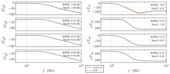
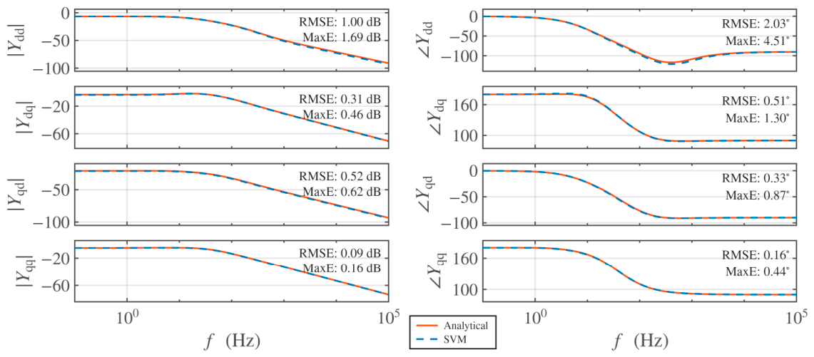
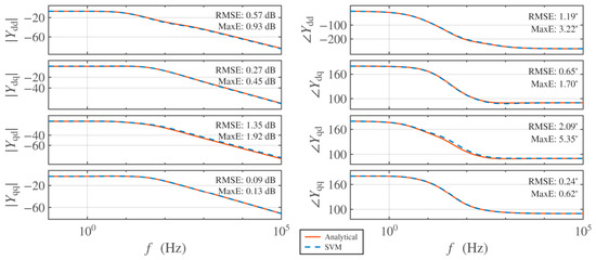
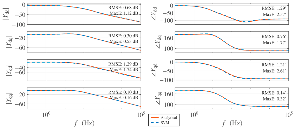
Figure 10 and Figure 11 illustrate the comparison between the true derived admittance and the SVM-predicted admittance under nominal grid voltage scenarios (fixed $V=1.0$ p.u.). Two random test cases are presented: Case $\mathrm{V}\_\mathrm{Fixed}\_3$ with the operating point $\mathit{x}={[-0.4759,-0.7818,1.0000,0.0969]}^{\mathrm{T}}$, and Case $\mathrm{V}\_\mathrm{Fixed}\_5$ with $\mathit{x}={[-0.8699,-0.8060,1.0000,-0.1736]}^{\mathrm{T}}$. As observed in the Bode plots, the predicted admittance tightly tracks the true model across the entire ultra-wide frequency band (0.1 Hz to 100 kHz). It is particularly noteworthy that the high fidelity is strictly maintained in the crucial low-frequency range (1–50 Hz). Since this specific band dictates the occurrences of sub-synchronous oscillations (SSO) in PMSG systems, the exact replication of resonance peaks and phase angles guarantees the reliability of subsequent stability margin assessments.

Figure 10. Results of Case $\mathrm{V}\_\mathrm{Fixed}\_3$ in the ideal grid.

Figure 11. Results of Case $\mathrm{V}\_\mathrm{Fixed}\_5$ in the ideal grid.

5.3.3. Prediction Under the Weak Grid Scenario

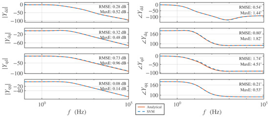
To further validate the robustness of the highly nonlinear mapping, Figure 12 and Figure 13 depict the prediction performance under voltage-varying conditions, representative of non-ideal weak grid environments. The tested operating points are $\mathrm{V}\_\mathrm{Var}\_1$ with $\mathit{x}={[-0.7643,-0.5704,0.8522,0.0835]}^{\mathrm{T}}$, and $\mathrm{V}\_\mathrm{Var}\_3$ with $\mathit{x}={[-0.7346,-0.8829,1.0845,0.1471]}^{\mathrm{T}}$. Despite the substantial deviations imposed on the PCC voltage, the equivalent-circuit topology equipped with SVM regressions reproduces the analytical admittance profiles with low errors, indicating its good generalization performance under the tested conditions in the presence of grid disturbances.

Figure 12. Results of Case $\mathrm{V}\_\mathrm{Var}\_1$ in the weak grid.

Figure 13. Results of Case $\mathrm{V}\_\mathrm{Var}\_3$ in the weak grid.

5.3.4. Quantitative Error Validation

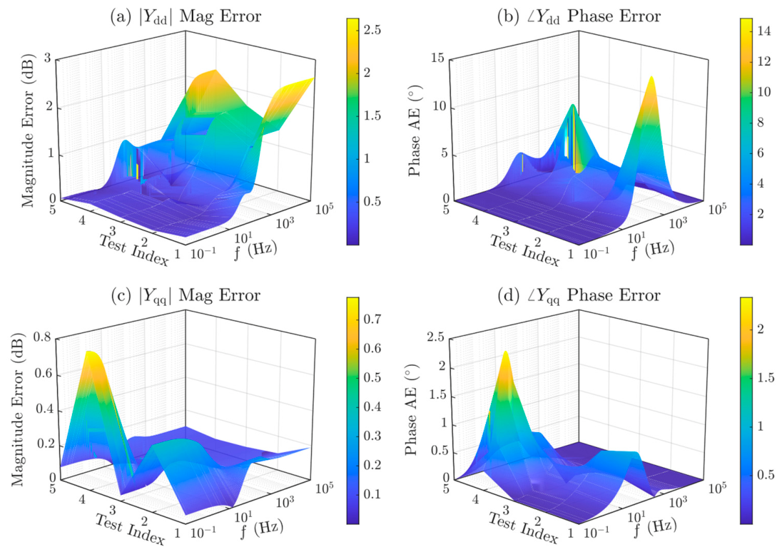
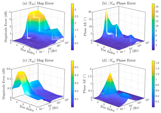
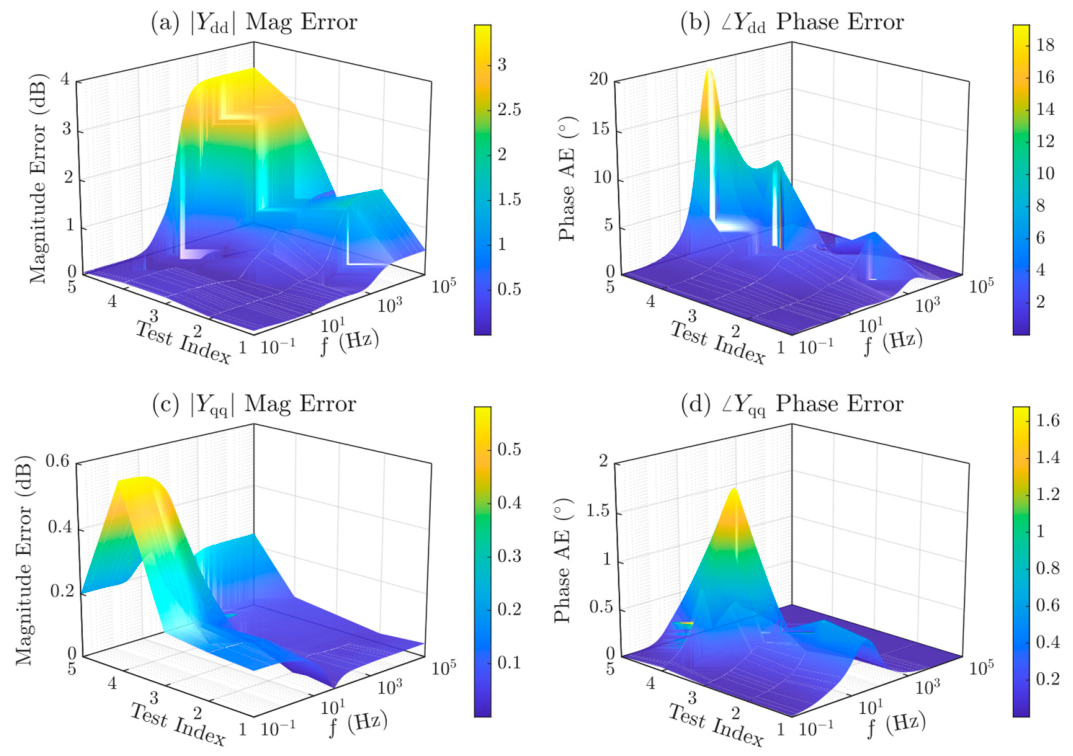
To conduct a rigorous statistical performance evaluation, Figure 14 and Figure 15 quantitatively characterize the absolute error (AE) between the predicted and reference values of the diagonal admittance components, i.e., $Y_{\mathrm{dd}}$ and $Y_{\mathrm{qq}}$.

Figure 14. Absolute errors of the predicted $Y_{\mathrm{dd}}$ and $Y_{\mathrm{qq}}$ of PMSG for the 5 random tests in the ideal grid: (a) $\left|Y_{\mathrm{dd}}\right|$, (b) $\angle Y_{\mathrm{dd}}$, (c) $\left|Y_{\mathrm{qq}}\right|$, and (d) $\angle Y_{\mathrm{qq}}$.

Figure 15. Absolute errors of the predicted $Y_{\mathrm{dd}}$ and $Y_{\mathrm{qq}}$ of PMSG for 5 tests in the weak grid: (a) $\left|Y_{\mathrm{dd}}\right|$, (b) $\angle Y_{\mathrm{dd}}$, (c) $\left|Y_{\mathrm{qq}}\right|$, and (d) $\angle Y_{\mathrm{qq}}$.

AE includes amplitude error and phase absolute error. For the admittance response at frequency $f_k$, let $Y_{\mathrm{pred}}\left(f_k\right)$ and $Y_{\mathrm{act}}\left(f_k\right)$ denote the predicted and reference admittance values, respectively.

The magnitude error in decibels (dB) is defined as

$$E_{\mathrm{mag}}\left(f_k\right)=\left|20{\log }_{10}\left|Y_{\mathrm{pred}}\right(f_k)|-20{\log }_{10}{|\mathrm{Y}}_{\mathrm{act}}{(\mathrm{f}}_{\mathrm{k}})|\right|.$$

(18)

This metric evaluates the deviation between the predicted and actual admittance magnitudes in the logarithmic frequency domain.

The phase absolute error is defined as

$$E_{\mathrm{phase}}(f_k)=\left|\mathrm{WrapTo}180\left(\angle \left({\displaystyle \frac{Y_{\mathrm{pred}}\left(f_k\right)}{Y_{\mathrm{act}}\left(f_k\right)}}\right)\cdot {\displaystyle \frac{180}{\pi }}\right)\right|,$$

(19)

where $\mathrm{WrapTo}180(\cdot )$ constrains the phase difference within the interval $[{-180}^{°},{180}^{°}]$ to avoid nonphysical discontinuities caused by phase wrapping.

Specifically, Figure 14 presents the error results under the ideal grid scenario, where subplots in Figure 14a,b illustrate the AE of the magnitude and phase of $Y_{\mathrm{dd}}$, respectively, while subplots in Figure 14c,d correspond to the AE results of the magnitude and phase of $Y_{\mathrm{qq}}$. Similarly, Figure 15 depicts the detailed error distributions for the aforementioned metrics under the weak grid scenario. Comprehensive analytical results confirm that the predicted AE remains low. For instance, within the low-to-medium frequency range under both scenarios, the AE of the magnitude and phase for both $Y_{\mathrm{dd}}$ and $Y_{\mathrm{qq}}$ fall into a limited range. Such minimal prediction deviations indicate that the methodology for mapping frequency-domain regression results to static equivalent-circuit parameter predictions can achieve high prediction accuracy identification and prediction of the AM for PMSG.

To further quantify the prediction accuracy of the proposed method, Table 6 lists the magnitude and phase errors of the Ydd admittance channel for the representative cases presented in Section 5.3.2 and Section 5.3.3. The reported metrics include the root mean square error (RMSE), mean absolute error (MAE), and maximum error for both magnitude and phase. As shown in Table 6, the proposed model achieves consistently low prediction errors for these representative cases.

Table 6. Quantitative prediction errors of the $Y_{\mathrm{dd}}$ admittance channel for the representative cases shown in Section 5.3.2 and Section 5.3.3.

Case	Mag_RMSE	Mag_MAE	Mag_Max_Error	Phase_RMSE	Phase_MAE	Phase_Max_Error
V_Fixed_3	1.00	0.73	1.69	2.03	1.34	4.51
V_Fixed_5	0.57	0.46	0.93	1.19	0.65	3.22
V_Var_1	0.28	0.21	0.52	0.54	0.37	1.44
V_Var_3	0.68	0.52	1.12	1.29	0.94	2.57

5.3.5. Impact of Training Dataset Size on Prediction Accuracy

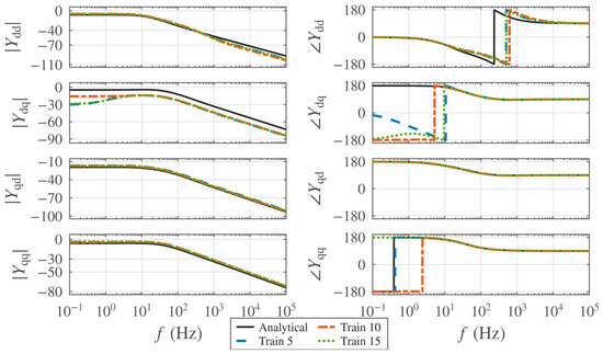
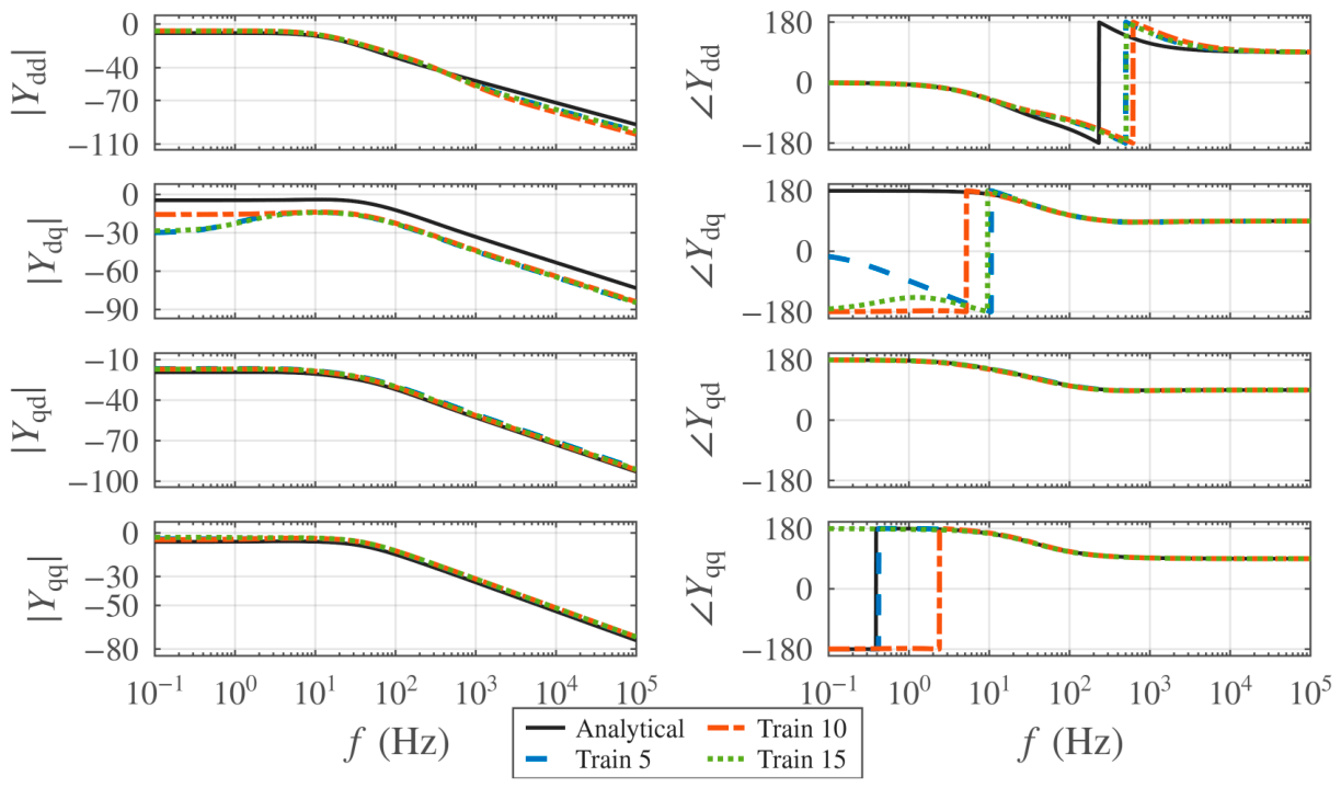
This subsection further evaluates the predictive performance of the proposed SVM-based AM by investigating the impact of varying training dataset sizes. The evaluated datasets are constructed by discretizing the active power ($P$) operating range into 5, 10 (the default configuration used throughout this paper), and 15 grid points. In comparison, the other three operating variables are consistently set to the default of 10 grid points. A comparative case study is conducted, focusing on PMSG performance under the conditionally selected V_Fixed_4 testing scenario. To ensure a rigorous and fair comparison, the SVM models trained on varying dataset scales use identical training methodologies and hyperparameter settings. Figure 16 illustrates the comparative results between the analytical and predicted AMs derived from the three training scales. As observed, the model trained with 10 grid points for $P$ achieves the optimal prediction accuracy. In contrast, the performance degrades to varying degrees when adopting either 5 or 15 grid points. This non-monotonic trend suggests that a sparse sampling grid (5 points) provides insufficient data to fully capture the system dynamics. Conversely, scaling up to an overly dense grid (15 points) tends to cause the model to overfit to localized variations, especially under fixed hyperparameter constraints. Consequently, rather than a simple linear tradeoff, appropriately selecting the dataset sampling granularity is critical; the 10-grid-point configuration offers the optimal balance between dataset generation cost and robust model generalization in practical engineering applications.

Figure 16. Impacts of varied training dataset sizes (5, 10, and 15 OPs) on the predicted AM using the proposed SVM-based approach.

5.3.6. Comparison with Alternative Regression Models and Rationale for Selecting SVR

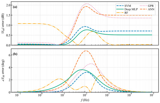
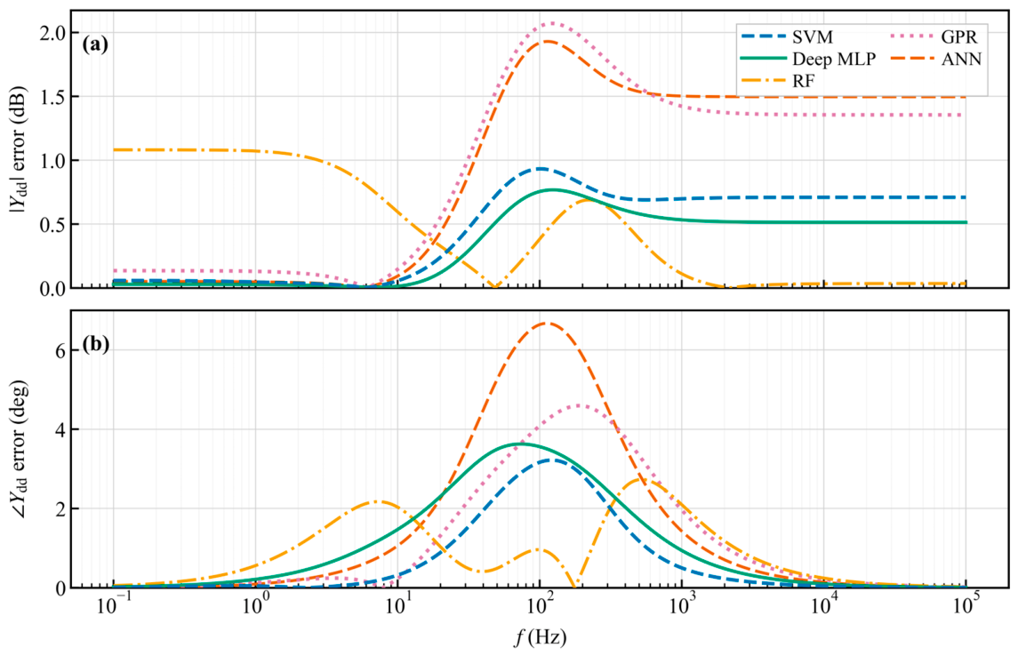
To further justify the selection of the SVM-based predictor, a comparative study was conducted using the $Y_{dd}$ channel of the admittance matrix as a representative example. Five regression models were considered, including SVM, ANN, Deep MLP, Gaussian Process Regression (GPR), and Random Forest (RF). All models were evaluated and compared at the same representative operating point, in terms of magnitude error, phase error, prediction time, saved model size, and peak resident-set-size (RSS) increase.

Figure 17 compares the frequency-domain errors of the $Y_{dd}$ responses reconstructed using different regression models. The results indicate that no single model achieves the best performance across all accuracy metrics: In terms of magnitude reconstruction, Deep MLP gives the lowest error, with a magnitude RMSE of 0.4352 dB, followed by SVM and RF with RMSE values of 0.5669 dB and 0.6314 dB, respectively. However, for phase reconstruction, SVM provides the lowest phase RMSE and MAE, namely 1.1863 deg and 0.6547 deg. RF gives the smallest maximum phase error of 2.7332 deg, but its average phase error is higher than that of SVM. ANN and GPR exhibit larger overall reconstruction errors than SVM and Deep MLP for this representative operating point. These results suggest that Deep MLP is advantageous in magnitude reconstruction, whereas SVM provides more favorable average phase accuracy. Therefore, the SVM-based predictor should not be interpreted as uniformly superior to all alternatives, but rather as a competitive option with balanced reconstruction accuracy, particularly for phase-sensitive admittance analysis.

Figure 17. Frequency-domain reconstruction errors of $Y_{dd}$ for different regression models at the representative operating point. The upper panel (a) shows the magnitude error in dB, and the lower panel (b) shows the phase error in degrees.

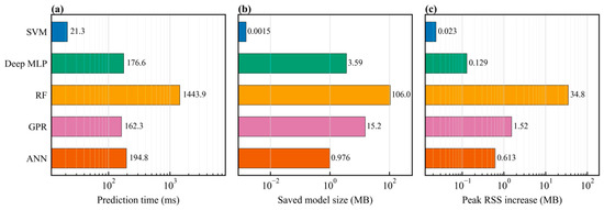
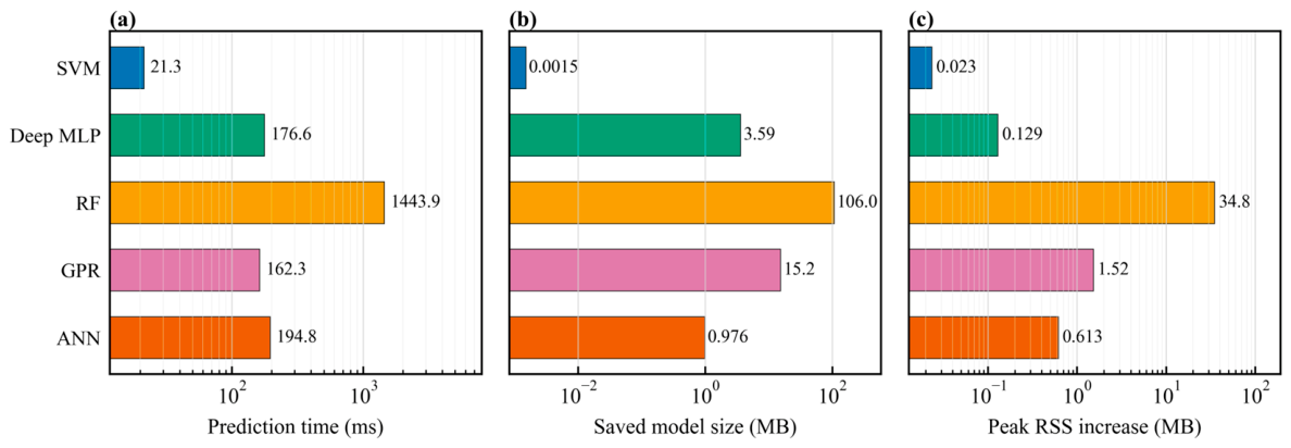
In addition to reconstruction accuracy, computational cost and memory requirement were evaluated to assess the feasibility of online or large-scale admittance prediction. As shown in Figure 18, SVM requires the shortest prediction time, the smallest saved model size, and the lowest peak memory increase among the compared models. Specifically, the SVM prediction time is 21.340 ms, with a saved model size of only 0.001495 MB and a peak RSS increase of 0.023438 MB. By contrast, Deep MLP achieves the lowest magnitude error but requires a larger model size of 3.589550 MB and a longer prediction time of 176.607 ms. RF obtains a relatively low maximum phase error, but its computational burden is considerably higher, with a prediction time of 1443.930 ms, a saved model size of 106.045 MB, and a peak RSS increase of 34.824 MB. GPR and ANN also require larger model sizes and memory footprints than SVM. These observations show that, although SVM is not the most accurate model in every error metric, it provides the most compact model representation and the lowest computational overhead in this comparison. Thus, SVM offers a favorable trade-off between frequency-domain reconstruction accuracy and deployment efficiency for the considered equivalent-circuit-parameter prediction task.

Figure 18. Computational-resource comparison among different regression models for $Y_{dd}$ reconstruction: (a) prediction time, (b) saved model size, and (c) peak resident-set-size increase during prediction.

6. Discussion

The proposed modeling framework, which integrates equivalent-circuit conversion with SVM-based prediction, offers a new perspective on admittance prediction and modeling. Instead of mapping steady-state operating points (OPs) to a high-dimensional data space comprising many discrete frequency points, the proposed method maps them to equivalent-circuit parameters, thereby avoiding the curse of dimensionality inherent in conventional black-box machine learning approaches. Consequently, the proposed strategy requires a significantly smaller training dataset while still achieving high-fidelity prediction. Moreover, it enables the derivation of broadband admittance characteristics across the entire frequency range, thereby avoiding interpolation errors and the limitations of narrowband modeling.

Furthermore, unlike purely data-driven black-box neural networks, the proposed synthesized equivalent-circuit model inherently preserves physical interpretability. The constructed resistive, inductive, and capacitive elements all have clear physical meanings, providing insights into the system’s dynamic interaction characteristics and its passive and active behavior across different frequency bands.

Despite its robust performance in the tested cases and analytical advantages, the proposed method still exhibits certain limitations in terms of data dependence. As a fundamental characteristic of data-driven mapping strategies, the prediction accuracy and generalization capability of the SVM-based parameter estimator inherently depend on the completeness of the training dataset. To ensure reliable generalization performance, the selected operating points must adequately cover the target operating range, especially when the system operates near nonlinear stability boundaries or under extreme grid conditions, where the internal control dynamics may undergo topological changes. If these critical regions are insufficiently sampled, the prediction accuracy of the equivalent-circuit parameters under a fixed topology may be adversely affected.

It should be emphasized that, although this paper uses the PMSG as a specific case to validate the effectiveness of the proposed framework, its underlying mathematical topology and circuit synthesis principles are, in theory, not restricted to any particular device type. By decoupling complex frequency-domain responses into physically meaningful equivalent circuits and further enabling low-dimensional mapping, the proposed method has broad potential for application to power-electronic-grid-interfaced equipment characterized by frequency-domain terminal behavior. Future work will focus on extending this unified modeling framework to heterogeneous topologies, such as GFM converters and high-voltage direct current (HVDC) systems, to further verify its practical applicability.

In addition, future research will build on this work to investigate the relationship between operating conditions and variations in equivalent-circuit element parameters, to identify their analytical models. This is expected to support real-time online admittance-based stability assessment of power systems with high penetration of renewable energy sources.

7. Conclusions

This paper proposes a highly efficient, physics-interpretable dimensionality-reduction and prediction framework for the wideband AM of a PMSG under varying operating conditions. The key findings of this work are summarized as follows:

• The occurrence of negative equivalent resistance or inductance indicates that the fitted terminal admittance contains non-passive small-signal characteristics in certain frequency ranges. These parameters should be regarded as behavioral equivalents of active converter-control dynamics, rather than as physical negative components in the PMSG hardware.
• By establishing the prediction model in terms of equivalent-circuit element parameters, the dimensionality of the output space is reduced, thereby alleviating the computational burden.
• By applying the inverse transformation to the newly predicted element parameters, the admittance under unseen OPs can be reconstructed, thereby enabling continuous characterization over the entire frequency range.

References

- Hatziargyriou, N.; Milanovic, J.; Rahmann, C.; Ajjarapu, V.; Canizares, C.; Erlich, I.; Hill, D.; Hiskens, I.; Kamwa, I.; Pal, B.; et al. Definition and Classification of Power System Stability—Revisited & Extended. IEEE Trans. Power Syst. 2021, 36, 3271–3281. [Google Scholar] [CrossRef] [Scilit]
- Buticchi, G.; Lam, C.-S.; Xinbo, R.; Liserre, M.; Barater, D.; Benbouzid, M.; Gomis-Bellmunt, O.; Ramos-Paja, C.A.; Kumar, C.; Zhu, R. The Role of Renewable Energy System in Reshaping the Electrical Grid Scenario. IEEE Open J. Ind. Electron. Soc. 2021, 2, 451–468. [Google Scholar] [CrossRef] [Scilit]
- Luo, J.; Liu, B.; Guo, X.; Yang, L.; Liu, C.; Xu, Y.; Bu, S. Oscillation stability induced by wind power integration: Incidents, mechanism, countermeasures and future challenges. Renew. Sustain. Energy Rev. 2025, 217, 115692. [Google Scholar] [CrossRef] [Scilit]
- Cheng, Y.; Fan, L.; Rose, J.; Huang, S.-H.; Schmall, J.; Wang, X.; Xie, X.; Shair, J.; Ramamurthy, J.R.; Modi, N.; et al. Real-World Subsynchronous Oscillation Events in Power Grids with High Penetrations of Inverter-Based Resources. IEEE Trans. Power Syst. 2023, 38, 316–330. [Google Scholar] [CrossRef] [Scilit]
- Zhan, Y.; Luo, Y.; Wang, L.; Xie, X. Interpretable data-driven method for sub/super-synchronous oscillation stability evaluation. Electr. Power Syst. Res. 2025, 241, 111399. [Google Scholar] [CrossRef] [Scilit]
- Kalcon, G.O.; Adam, G.P.; Anaya-Lara, O.; Lo, S.; Uhlen, K. Small-Signal Stability Analysis of Multi-Terminal VSC-Based DC Transmission Systems. IEEE Trans. Power Syst. 2012, 27, 1818–1830. [Google Scholar] [CrossRef] [Scilit]
- Sun, J. Impedance-Based Stability Criterion for Grid-Connected Inverters. IEEE Trans. Power Electron. 2011, 26, 3075–3078. [Google Scholar] [CrossRef] [Scilit]
- Pape, M.; Kazerani, M. A Generic Power Converter Sizing Framework for Series-Connected DC Offshore Wind Farms. IEEE Trans. Power Electron. 2021, 37, 2307–2320. [Google Scholar] [CrossRef] [Scilit]
- Luo, J.; Wang, P.; Zhao, H.; Liu, Y.; Terzija, V. Online identification of stability region for large-scale wind farms, Part II: Construction of stability region boundary. Int. J. Electr. Power Energy Syst. 2025, 169, 110790. [Google Scholar] [CrossRef] [Scilit]
- Zhou, W.; Torres-Olguin, R.E.; Gothner, F.; Beerten, J.; Zadeh, M.K.; Wang, Y.; Chen, Z. A Robust Circuit and Controller Parameters’ Identification Method of Grid-Connected Voltage-Source Converters Using Vector Fitting Algorithm. IEEE J. Emerg. Sel. Top. Power Electron. 2022, 10, 2748–2763. [Google Scholar] [CrossRef] [Scilit]
- Wang, L.; Qin, Z.; Bauer, P. A Gradient-Descent Optimization Assisted Gray-Box Impedance Modeling of EV Chargers. IEEE Trans. Power Electron. 2023, 38, 8866–8879. [Google Scholar] [CrossRef] [Scilit]
- Nahalparvari, M.; Asoodar, M.; Jahn, I.; Bessegato, L.; Despouys, O.; Norrga, S.; Nee, H.-P. DC-Side Impedance Estimation of a Modular Multilevel Converter Through System Identification of a Partially Black-Boxed Control System. IEEE Trans. Energy Convers. 2022, 37, 2708–2721. [Google Scholar] [CrossRef] [Scilit]
- Liao, Y.; Wu, H.; Wang, X.; Ndreko, M.; Dimitrovski, R.; Winter, W. Stability and Sensitivity Analysis of Multi-Vendor, Multi-Terminal HVDC Systems. IEEE Open J. Power Electron. 2023, 4, 52–66. [Google Scholar] [CrossRef] [Scilit]
- Li, Y.; Wu, X.; Shuai, Z.; Zhou, Q.; Chen, H.; Shen, Z.J. A Systematic Stability Enhancement Method for Microgrids With Unknown-Parameter Inverters. IEEE Trans. Power Electron. 2023, 38, 3029–3043. [Google Scholar] [CrossRef] [Scilit]
- Liao, Y.; Li, Y.; Chen, M.; Nordström, L.; Wang, X.; Mittal, P.; Poor, H.V. Neural Network Design for Impedance Modeling of Power Electronic Systems Based on Latent Features. IEEE Trans. Neural Netw. Learn. Syst. 2024, 35, 5968–5980. [Google Scholar] [CrossRef] [Scilit]
- Liu, W.; Xie, X.; Shair, J.; Li, X. A Nearly Decoupled Admittance Model for Grid-Tied VSCs Under Variable Operating Conditions. IEEE Trans. Power Electron. 2020, 35, 9380–9389. [Google Scholar] [CrossRef] [Scilit]
- Qiu, Q.; Huang, Y.; Ma, R.; Kurths, J.; Zhan, M. Black-Box Impedance Prediction of Grid-Tied VSCs Under Variable Operating Conditions. IEEE Access 2022, 10, 1289–1304. [Google Scholar] [CrossRef] [Scilit]
- Liu, W.; Xie, X.; Shair, J.; Liu, H.; He, J. Frequency-coupled impedance model-based sub-synchronous interaction analysis for direct-drive wind turbines connected to a weak AC grid. IET Renew. Power Gener. 2019, 13, 2966–2976. [Google Scholar] [CrossRef] [Scilit]
- Gbadega, P.A.; Sun, Y.; Balogun, O.A. Optimized energy management in Grid-Connected microgrids leveraging K-means clustering algorithm and Artificial Neural network models. Energy Convers. Manag. 2025, 336, 119868. [Google Scholar] [CrossRef] [Scilit]
- Xiao, P.; Venayagamoorthy, G.K.; Corzine, K.A.; Huang, J. Recurrent Neural Networks Based Impedance Measurement Technique for Power Electronic Systems. IEEE Trans. Power Electron. 2010, 25, 382–390. [Google Scholar] [CrossRef] [Scilit]
- Zhang, M.; Wang, X.; Yang, D.; Christensen, M.G. Artificial Neural Network Based Identification of Multi-Operating-Point Impedance Model. IEEE Trans. Power Electron. 2021, 36, 1231–1235. [Google Scholar] [CrossRef] [Scilit]
- Zhang, M.; Wang, X.; Yang, D.; Cui, Z.; Christensen, M.G. Transfer Learning for Identifying Impedance Estimation in Voltage Source Inverters. In Proceedings of the 2020 IEEE Energy Conversion Congress and Exposition (ECCE), Detroit, MI, USA, 11–15 October 2020; pp. 6170–6174. [Google Scholar] [CrossRef] [Scilit]
- Zhang, M.; Zhang, Y.; Xu, Q. Transfer Learning Based Online Impedance Identification for Modular Multilevel Converters. IEEE Trans. Power Electron. 2023, 38, 12207–12218. [Google Scholar] [CrossRef] [Scilit]
- Li, Y.; Liao, Y.; Wang, X.; Nordstrom, L.; Mittal, P.; Chen, M.; Poor, H.V. Neural Network Models and Transfer Learning for Impedance Modeling of Grid-Tied Inverters. In Proceedings of the 2022 IEEE 13th International Symposium on Power Electronics for Distributed Generation Systems (PEDG), Kiel, Germany, 26–29 June 2022; pp. 1–6. [Google Scholar] [CrossRef] [Scilit]
- Li, H.; Nian, H.; Zhan, L.; Hu, B.; Li, M. Few-Shot Data-Driven Modeling of Unified Grid Tied VSCs for Multioperation Impedance Identification Based on PINN. IEEE Trans. Ind. Electron. 2025, 72, 6957–6968. [Google Scholar] [CrossRef] [Scilit]
- Zhang, M.; Xu, Q.; Wang, X. Physics-Informed Neural Network Based Online Impedance Identification of Voltage Source Converters. IEEE Trans. Ind. Electron. 2023, 70, 3717–3728. [Google Scholar] [CrossRef] [Scilit]
- Mohammed, N.; Zhou, W.; Bahrani, B.; Hill, D.J. Support Vector Machines for Predicting the Impedance Model of Inverter-Based Resources. IEEE Trans. Power Syst. 2024, 39, 7359–7375. [Google Scholar] [CrossRef] [Scilit]
- Ali, M.; Mohamed, Y.A.-R.I. Dropout Kolmogorov–Arnold Networks: A Novel Data-Driven Impedance Modeling Approach for Voltage-Source Converters. IEEE Open J. Power Electron. 2025, 6, 562–582. [Google Scholar] [CrossRef] [Scilit]
- Wang, Y.; Li, H.; Zhang, F.; He, Z.; Zhang, J.; Nian, H. Data-Driven Modeling Method of Multi-Operation Impedance Identification for DFIG Based on Transfer Learning Theory. In Proceedings of the 2024 CPSS & IEEE International Symposium on Energy Storage and Conversion (ISESC), Xi’an, China, 8–11 November 2024; pp. 377–382. [Google Scholar] [CrossRef] [Scilit]
- Zhang, Z.; Wu, W.; Xie, Z.; Chen, Y.; Cao, S.; Luo, C. Identification Modeling of Frequency-Coupling Admittance for Grid-Connected Inverter Under All Operating Conditions. In Proceedings of the 2023 IEEE 6th International Electrical and Energy Conference (CIEEC), Hefei, China, 12–14 May 2023; pp. 2434–2439. [Google Scholar] [CrossRef] [Scilit]
- Gustavsen, B.; Semlyen, A. Rational approximation of frequency domain responses by vector fitting. IEEE Trans. Power Deliv. 1999, 14, 1052–1061. [Google Scholar] [CrossRef] [Scilit]
- Gustavsen, B. Improving the Pole Relocating Properties of Vector Fitting. IEEE Trans. Power Deliv. 2006, 21, 1587–1592. [Google Scholar] [CrossRef] [Scilit]
- Deschrijver, D.; Mrozowski, M.; Dhaene, T.; De Zutter, D. Macromodeling of Multiport Systems Using a Fast Implementation of the Vector Fitting Method. IEEE Microw. Wirel. Compon. Lett. 2008, 18, 383–385. [Google Scholar] [CrossRef] [Scilit]
- Knockaert, L.; Ferranti, F.; Dhaene, T. Vector Fitting vs. Levenberg-Marquardt: Some experiments. In Proceedings of the 2009 IEEE Workshop on Signal Propagation on Interconnects, Strasbourg, France, 12–15 May 2009; pp. 1–4. [Google Scholar] [CrossRef] [Scilit]
- Xiong, Y.; Li, X.; Li, Y.; Zhao, X. A High-frequency Motor Model Constructed Based on Vector Fitting Method. In Proceedings of the 2019 Joint International Symposium on Electromagnetic Compatibility, Sapporo and Asia-Pacific International Symposium on Electromagnetic Compatibility (EMC Sapporo/APEMC), Sapporo, Japan, 3–7 June 2019; pp. 191–194. [Google Scholar] [CrossRef] [Scilit]
- Cortes, C.; Vapnik, V. Support-vector networks. Mach. Learn. 1995, 20, 273–297. [Google Scholar] [CrossRef] [Scilit]
- Drucker, H.; Burges, C.; Kaufman, L.; Smola, A.; Vapnik, V. Support vector regression machines. Adv. Neural Inf. Process. Syst. 1997, 28, 779–784. [Google Scholar]
- Noble, W.S. What is a support vector machine? Nat. Biotechnol. 2006, 24, 1565–1567. [Google Scholar] [CrossRef] [Scilit]
- Burges, C.J.C. A Tutorial on Support Vector Machines for Pattern Recognition. Data Min. Knowl. Discov. 1998, 2, 121–167. [Google Scholar] [CrossRef] [Scilit]
- Ali, M.; Fissha, Y. Propose adjustable Support Vector Machine approach for classifying imbalanced work travel mode choice data. Transp. Res. Interdiscip. Perspect. 2026, 35, 101786. [Google Scholar] [CrossRef] [Scilit]
- Cervantes, J.; Garcia-Lamont, F.; Rodríguez-Mazahua, L.; Lopez, A. A comprehensive survey on support vector machine classification: Applications, challenges and trends. Neurocomputing 2020, 408, 189–215. [Google Scholar] [CrossRef] [Scilit]
- IEEE Std 1547-2018; IEEE Standard for Interconnection and Interoperability of Distributed Energy Resources with Associated Electric Power Systems Interfaces. IEEE: New York, NY, USA, 2018.
- AS/NZS 4777.1:2024; Grid Connection of Energy Systems via Inverters—Part 1: Installation Requirements. Standards Australia Limited: Sydney, Australia; Standards New Zealand: Wellington, New Zealand, 2024.
- AS/NZS 4777.2:2020; Grid Connection of Energy Systems via Inverters—Part 2: Inverter Requirements. Standards Australia Limited: Sydney, Australia; Standards New Zealand: Wellington, New Zealand, 2020.
- GB/T 19963.1-2021; Technical Requirements for Connecting Photovoltaic Power Station to Power System—Part 1: General Requirement. State Administration for Market Regulation: Beijing, China; Standardization Administration of the People’s Republic of China: Beijing, China, 2021.
Disclaimer/Publisher’s Note: The statements, opinions and data contained in all publications are solely those of the individual author(s) and contributor(s) and not of MDPI and/or the editor(s). MDPI and/or the editor(s) disclaim responsibility for any injury to people or property resulting from any ideas, methods, instructions or products referred to in the content. |
© 2026 by the authors. Licensee MDPI, Basel, Switzerland. This article is an open access article distributed under the terms and conditions of the Creative Commons Attribution (CC BY) license.