


Abstract
Driver drowsiness is a major cause of fatal car accidents, and camera-based monitoring offers a promising way to detect it. Detecting drowsiness from video requires modeling both facial appearance and its temporal evolution. In this article, we propose MSCT-Net, a multi-stream CNN–Transformer network for this purpose. Region-specific CNN backbones encode the face, right eye and mouth in every frame. Then, a single Transformer encoder jointly models their temporal dynamics across regions and time. MSCT-Net is trained from scratch on the challenging NTHU Drowsy Driver Detection dataset, which covers daytime and nighttime driving with and without eyewear. The architectures for the backbones and the Transformer are selected experimentally on the validation set. Compared with a baseline that shares the same backbones but averages features over time, MSCT-Net improves the clip-level accuracy from 78.70% to 82.16%, the F1-score from 81.15% to 83.15% and the AUC from 0.8807 to 0.9052, with higher accuracy and AUC in every scenario of the dataset. It also outperforms a CNN-LSTM baseline of similar size (accuracy 80.94%, F1-score 82.79%, AUC 0.8983). On the official test set of 14 subjects, MSCT-Net achieves a frame-level accuracy of 82.26% without any post-processing.
1. Introduction
Driver’s fatigue is one of the major causes of car accidents worldwide [1,2]. Fatigue develops gradually and arises not only from driving conditions but also from the driver’s own mental and physiological state. It leads to a decline in cognitive performance and reduces decision-making abilities. Moreover, it induces drowsiness, which is regarded as a transition from alertness to sleep and is directly associated with increased risk of accidents. To improve road safety and reduce road accidents, an automated system to detect driver drowsiness is highly desired which is destined to alert the driver when he/she enters the drowsiness state.
Among the various drowsiness detection approaches, ranging from techniques that analyze biological signals to those that rely on the imaging-based sensing, camera-based methods have shown great potential as they are non-intrusive, inexpensive and easy to deploy. In their simplest form, a camera captures driver’s face and vision-based algorithms track head movements and observe behavioral cues such as blink duration, eyelid closure and yawning to determine the drowsiness state. However, building robust vision-based algorithms for this task is quite challenging due to unrestricted head pose variations, changing illumination conditions, occlusions and the need to accurately capture facial cues associated with drowsiness [3]. Given the challenges, the design and development of robust vision-based algorithms for drowsiness detection have been a major research focus in the past decade within the fields of computer vision and intelligent transportation systems [4]. In this article, we address this modality.
As mentioned earlier, drowsiness emerges from motion cues such as eye closure spanning over several hundred milliseconds, a blink rate that climbs steadily over minutes and yawning lasting several seconds; a single frame from a video sequence cannot capture these cues and therefore spatiotemporal models are well suited for detecting drowsiness. Among such approaches, deep-learning-based models are quite popular for drowsiness detection as well as for vision tasks involving videos, since their end-to-end learning paradigm eliminates the need for hand-crafted appearance and motion features. Pioneering works on deep spatiotemporal networks extended convolutional neural networks (CNNs) in different ways. Two-stream networks [5] use an optical flow stream in addition to an RGB image stream to capture motion cues end to end. Three-dimensional CNNs [6] extend convolutions into the temporal dimension so that spatial and temporal filters are learned jointly, without the need of a separate optical flow stream. I3D [7] expands pretrained 2D convolutional filters into spatiotemporal kernels by replicating them along the time dimension. The resulting 3D network is then fine-tuned to perform video action recognition. The use of pretrained CNNs on large-scale datasets such as ImageNet has helped close the performance gap between video and image models. Rather than extending convolution into the temporal dimension, recurrent neural networks (RNNs) provide an alternative way to model temporal dynamics. Long-Term Recurrent Convolutional Networks (LRCN) [8] are an example of this approach where a CNN backbone generates a fixed-length feature vector for each frame, and a stack of Long Short-Term Memory (LSTM) units then encodes the temporal information for a sequence of frames. These developments have also helped in the design of spatiotemporal models for drowsiness detection in videos. In [9], a Hierarchical Temporal Deep Belief Network (HTDBN) was proposed that determines the drowsiness state by extracting temporal information from a sequence of face images. CNNs and their variants such as 3D CNNs have also been employed for drowsiness detection [10,11,12,13]. Similarly, RNN-based models, including LSTM variants, have also been proposed for the task [14,15,16]. These models have been found to perform reasonably well in determining the driver’s drowsiness state, but their performance remains limited by their ability to capture long-range temporal dependencies which is a common limitation of CNN- and RNN-based spatiotemporal models. Capturing long-range motion cues is crucial in drowsiness detection as they are associated with the gradual behavioral changes over time. Three-dimensional CNN models extract motion cues from a fixed, local temporal window with the help of 3D kernels, but their receptive field is limited to a finite range which prevents them from modeling long-range temporal dependencies. In contrast, RNN-based models propagate information through many recurrent units, which leads to temporal degradation over longer sequences due to vanishing gradients. Although LSTM’s gating mechanism is employed to overcome the vanishing gradient problem seen in traditional RNNs, it does not eliminate the degradation entirely for longer sequences.
In comparison to RNN-based architectures, the Transformer architecture [17], through its self-attention mechanism, offers an alternative approach to model long-range temporal dependencies. It also eliminates the need for recurrent paths and achieves high scalability. Moreover, it enables the model to compute contextual relationships across the entire sequence. The vision-based counterpart of Transformers, known as the Vision Transformer (ViT) [18], applies the same self-attention mechanism directly to image patches without the use of convolution filters. It has been shown to be superior or on par with the CNN-based architectures on various image-based tasks when trained on a sufficiently large-scale image dataset. TimeSformer [19] extends ViT to video classification by applying the self-attention mechanism across both spatial and temporal dimensions. It has shown to achieve competitive performance compared to 3D CNNs while being effective at handling longer sequences in video-based action recognition benchmarks. However, despite these advantages, training ViT-based models remains challenging on small datasets due to their weak inductive bias. To achieve adequate performance on limited data, both architecture and training scheme need to be designed carefully [20,21].
The Multi-stream CNN–Transformer network (MSCT-Net) proposed in this article for driver drowsiness detection in videos is motivated by the complementary strengths of CNNs and Transformers discussed above. Drowsiness detection relies on monitoring the face and facial regions for appearance and motion patterns, and we therefore adopt separate architectural components to model these two aspects. CNNs remain well suited to extracting appearance features from face and facial regions, so we employ a separate CNN backbone for each of the face, right eye and mouth streams to form a multi-stream network. Each backbone produces a compact feature vector for every frame in a video clip. To capture temporal dynamics such as eye-closure duration, yawning, and head tilt, a single Transformer encoder is applied jointly to the feature sequences of all three streams. The self-attention mechanism of the Transformer encoder enables the model to relate any frame of any region to any other and to learn both temporal patterns and dependencies across facial regions. This is different from existing multi-stream models where regions are fused frame by frame or only at the classification stage, resulting in an indirect interaction between different frames of different regions. The CLS embedding of the encoder is fed to a fully connected layer that classifies the clip as alert or drowsy. We train MSCT-Net from scratch using the challenging NTHU Drowsy Driver Detection dataset (NTHU-DDD) [9]. The backbones are simple, vanilla CNNs, and the Transformer encoder is shallow, so our proposed MSCT-Net has only about 3.6M parameters in total. As Transformers are prone to overfitting on small datasets [18], we employ strong image augmentations and regularization. Experiments on the official test set of the NTHU-DDD dataset, containing 14 subjects, show that MSCT-Net achieves a frame-level accuracy of 82.26% without any post-processing. In the following, we summarize the main contributions of our work:
- We propose MSCT-Net, which encodes the face, right eye and mouth with region-specific CNN backbones. A single shallow Transformer encoder then learns both temporal patterns and dependencies across all three regions. The model has only about 3.6M parameters and is trained from scratch.
- We compare MSCT-Net with a baseline that uses the same backbones and training but averages the features over time. The absolute gains of MSCT-Net in accuracy, F1-score and AUC are 3.5%, 2.0% and 0.025, respectively. Moreover, it outperforms the baseline in accuracy and AUC in every scenario of the dataset. MSCT-Net also outperforms a CNN-LSTM baseline with a comparable number of parameters on all three metrics.
- Our evaluation is based on the subject-disjoint official splits of NTHU-DDD, including the 14-subject test set. We also analyze the contribution of each facial stream and of the temporal window length. On the test set, MSCT-Net achieves a frame-level accuracy of 82.26% without any post-processing, comparable to that of an existing CNN-LSTM method that relies on temporal smoothing [22].
The rest of this article is organized as follows: Section 2 reviews existing methods and approaches for driver drowsiness detection in video. The details of the proposed hybrid CNN–Transformer model are presented in Section 3. Section 4 describes the NTHU dataset, implementation details, experimental results including the computational cost of MSCT-Net, an ablation study, a comparison with the existing methods and the limitations of this work. Finally, Section 5 concludes the article and outlines some future directions.
2. Related Works
Driver drowsiness detection is an active research problem within intelligent transportation systems. Three sensing paradigms have been proposed in the literature for the task: (1) direct monitoring of biological signals, including electrocardiograms (ECG) for heart rate variability, electromyograms (EMG) for muscle tone, electroencephalograms (EEG) for brain cortical activity and electrooculograms (EOG) for eye movement [23,24,25,26]; (2) contactless camera-based monitoring of visual fatigue indicators such as eyelid closure, blink rate, yawning, head tilting; and (3) non-intrusive monitoring of vehicle-based parameters, including lane deviations, steering wheel angle fluctuations, vehicle speed variances [27,28]. As this article focuses on vision-based sensing for driver drowsiness detection, we present a review of modern vision-based methods for the task. It is important to note that majority of recent methods for driver drowsiness detection are inspired by advances in deep learning. Such methods model driver’s state as a temporal sequence problem instead of static image classification problem, employing complex spatiotemporal architectures such as 3D-CNNs, CNN-LSTMs and ViTs to capture both spatial and temporal patterns of fatigue [3]. In addition to methods, several public benchmark datasets such as YawDD [29], NTHU-DDD, SUST-DDD [30], and ULDD [31] have been developed. Among them, NTHU-DDD is the most extensively used, as reflected in the literature reviewed below, due to its subject diversity and challenging conditions including illumination variations and occlusions.
In a pioneering work [9], Weng et al. propose a two-stage Hierarchical Temporal Deep Belief Network (HTDBN). In the first stage, geometric features from facial landmarks after 3D frontalization are fed to three separate Deep Belief Networks (DBNs) that compute region-specific motion probabilities for each frame. Pairwise landmark-point differences for the mouth and head, and average eye angle over a preceding time window for the eyes serve as the geometric features. The 3D frontalization offers robustness against head orientation prior to feature extraction. The resulting probability vectors form sequences that serve as the inputs to the second stage composed of two class-conditional continuous Hidden Markov Models (HMMs). These HMMs are trained on drowsy and non-drowsy sequences, respectively, and the accumulated likelihood difference between the two is transformed to yield a continuous drowsy score. The DBN-HMM architecture shows strong physiological interpretability by decoupling eye, mouth, and head motions. Moreover, unlike CNN-based approaches, which learn directly from pixel data in face or facial-region crops, this architecture operates on geometric features. Experimental results conducted on their proposed NTHU-DDD dataset show that the detection accuracy degrades substantially under sunglasses and nighttime conditions due to reflections and reduced facial-landmark accuracy.
Subsequent works have focused on replacing hand-crafted geometric features with learned spatiotemporal representations using 3D-CNN based encoders capable of modeling appearance and motion jointly. In [32], a condition-adaptive representation learning framework is proposed. The framework is composed of four major blocks: a 3D-CNN encoder for spatiotemporal feature extraction, a scene understanding module to predict the scene conditions including glasses/illumination, head, mouth and eye state, a feature fusion module and a final detection network. The scene understanding module uses the same spatiotemporal representation of the 3D-CNN for predicting the scene conditions. However, training of the module requires extra annotations regarding scene conditions beyond the drowsiness labels themselves. The framework achieves 76.2% average drowsiness detection accuracy on the NTHU-DDD evaluation set composed of 20 videos of four subjects. Kang et al. [12] proposed a 3D-CNN architecture using two facial regions and conducted a systematic search over the temporal window configuration. The authors propose using RetinaFace [33] to detect faces, along with five facial landmarks. The right eye and mouth regions are localized, aligned and warped to fixed 64 × 64 regions. Gamma correction with a target mean intensity of 128 and a separate contrast normalization stage to handle illumination variability are employed as preprocessing steps. Each facial region is then fed to a 3D-CNN network and the outputs of two streams are concatenated before the final classification layer. Models are trained using different temporal window sizes ranging from 5 to 128 frames and different frame overlaps. The best configuration, a temporal window of 10 with five-frame overlap, achieves an accuracy of 94.74% on the NTHU-DDD evaluation set. It is important to note that the authors select their best window and overlap by directly comparing accuracy across all evaluated configurations.
In contrast to 3D-CNNs where motion information is learned jointly with the appearance in an implicit manner, Shen et al. [11] propose using optical flow as a second input stream alongside appearance. The authors use three parallel two-stream networks for drowsiness detection in video clips. Each facial region (eyes, mouth and head) forms one stream of one of the two-stream networks while the corresponding optical flow forms the other stream. This scheme enables each two-stream network to capture both spatial and temporal patterns. The outputs of the parallel networks are concatenated and fed to a fully connected classification head for final decision. Before joint fine-tuning, each two-stream network is pretrained on the NTHU-DDD dataset separately. CLAHE is used in preprocessing to handle illumination variations. The parallel two-stream networks achieve an accuracy of 94.46% on a custom split of NTHU-DDD dataset.
Hybrid CNN-LSTM models separate spatial and temporal learning by employing a 2D CNN network for per-frame spatial features followed by an RNN-based network for temporal modeling. The Multistage Spatial-Temporal Network (MSTN) [22] uses a CNN (modified VGG-16 model) to extract spatial features from each frame and then uses LSTM to model the temporal evolution of the features. Finally, frame-level predictions are temporally smoothed to suppress noisy outputs. MSTN achieves an accuracy of 82.61% on the official NTHU-DDD test set. In [34], Long-Term Multi-Granularity Deep Framework (LMDF) is proposed. The CNN stage applies parallel CNNs as feature extractors to well-aligned facial patches from three granularities: global face, main parts (nose, eyes, mouth), and local regions, including the corners of the eyes and mouth and the sides of the nose. The resulting per-patch feature maps are concatenated into a high-dimensional feature vector and combined using a fully connected layer to output single spatial representation for each frame. A multi-layer LSTM stage models temporal patterns using these spatial representations across a sequence. A classification head then labels each frame as drowsy or non-drowsy. The method achieves 90.05% accuracy on the evaluation set of NTHU-DDD dataset. The experimental results on the static single-frame variant of the model show that the accuracy is highly sensitive to face landmark alignment precision. The authors also proposed to retrain a separate model for nighttime scenario rather than using a single model across daytime and nighttime scenarios. In a later work [16], a hybrid CNN-LSTM architecture is proposed which combines structural and spatial features. Specifically, six structural features (left/right eyes and eyebrows movements, mouth movements, head pose) extracted from 68-point Dlib facial landmarks [35] are used in the model. Moreover, classification decision score from the AlexNet is concatenated with the structural features to form a unified per-frame representation which is then fed to a four-layer LSTM over a 150-frame sequence for temporal modeling. A post-processing refinement process based on the consistency of prediction lasting tens of consecutive frames outputs the final decision. The method achieves 90.12% accuracy on combined NTHU-DDD evaluation and test set (18 subjects, 90 videos). The authors have found that structural features alone are particularly sensitive to illumination causing a decrease in accuracy in night-glasses scenario. Zhu et al. [36] proposed a two-stage framework that addresses both temporal modeling and inference efficiency. Facial and head pose features are extracted for each frame using YOLO and FSA-Net, respectively, to form two branches. In the first stage, a Temporal Dual-Stream Fusion (TDF) module uses Gated Recurrent Units to capture facial and head-pose dynamics. In the second stage, an adaptive feature selection mechanism dynamically executes the facial branch, the head-pose branch or both, based on a confidence score estimated from a single frame. The method achieves an accuracy of 96.07% at 56.96 frames per second on a custom subject-independent split of NTHU-DDD. Tüfekci et al. [14] formulate drowsiness detection as an anomaly detection problem and train an LSTM autoencoder on normal (non-drowsy) video clips only. A ResNet-34, pretrained on ImageNet and fine-tuned on the NTHU-DDD dataset, extracts a 512-dimensional feature vector for each frame which is then L2 normalized. Contrast Limited Adaptive Histogram Equalization (CLAHE) is used in preprocessing to enhance contrast in frames. The feature vectors of 3 s clips are fed into a two-layer LSTM encoder which converts them into a single spatiotemporal vector. A two-layer LSTM decoder reconstructs the features and reconstruction error is computed using mean square error (MSE), which served as the anomaly score. Anomalous clips yield higher reconstruction error and are therefore labeled as drowsy. The evaluation set of NTHU-DDD dataset is used to evaluate the model, achieving an accuracy and AUC of 81.79% and 87.40%, respectively. The recall and precision of the model are dependent on the choice of normal confidence labeling thresholds during training. For example, when low confidence normal clips are used during training, the model achieves high recall but poor precision.
In contrast to temporal-modeling approaches, frame-based deep classification models have also been proposed. Al-Gburi et al. [13] proposed EffRes-DrowsyNet framework, employing a pretrained EfficientNetB0 [37] and ResNet50 [38] as backbones. The features from both models are fused with the Eye Aspect Ratio (EAR) and Mouth Aspect Ratio (MAR) extracted via 68-point Dlib facial landmarks [35]. The backbones are fine-tuned on the training dataset along with a custom classification head. Experiments conducted on YawDD, SUST-DDD and NTHU-DDD datasets show that the framework achieves accuracies of 92.73%, 97.71%, and 95.14%, respectively. It is important to note that the framework uses a custom split for all datasets and performs frame-by-frame classification. Similarly, Vis-Net [39] categorizes a face image into one of the five drowsiness levels based on Kitajima’s scale. Face detection is achieved using YOLOv8 while the feature extraction stage employs different pretrained CNN backbones, including ResNet152, InceptionV3, DenseNet, NASNetLarge and MobileNetV2. The resulting features from a given backbone are fed to a ViT for classification. The Vis-Net is trained on 70% split of a custom dataset composed of 26,614 images with a 20% split held out for testing and rest for validation. The Vis-Net model achieved an accuracy of 98.94% on the test split. The authors have shown that the model is robust to face occlusions due to masks or glasses. The main limitation of the above-mentioned frame-based models is that they do not have a temporal component to observe the evolution of driver’s fatigue over time.
Unlike fully end-to-end deep learning pipelines, an alternative design choice uses a frozen backbone for features extraction followed by conventional machine learning classifiers. In [40] the authors propose a hybrid framework combining deep features, feature selection, and SVM classification. Tiny-YOLO is used for face detection followed by a frozen ResNet-50 pretrained on VGGFace2 to extract a 2048-dimensional feature vector per frame. A sliding window of nine frames is used to build a temporal window and per-frame features within the window are aggregated via mean and RMS statistics and then reduced to a compact representation using a hybrid feature selection method (FCFS). A linear SVM categorizes each temporal window or clip as drowsy or non-drowsy. Evaluated on the NTHU-DDD evaluation set with a single model spanning all five scenarios, the method achieves 86.74% overall accuracy. The framework also exhibits higher false positives than false negatives in most scenarios which the authors attribute to ambiguous drowsiness onset/offset frames.
In the majority of the deep learning-based works reviewed in this section, spatial feature extraction is performed by CNNs, while temporal modeling relies on either recurrent networks or 3D CNNs. Both 3D-CNN- and RNN-based approaches are limited in modeling long-range dependencies. Moreover, in the multi-stream methods presented above, the features of the facial regions for each frame are either concatenated into a single vector before the temporal modeling [16,34], or processed by separate networks whose outputs are fused only at the final classification stage [11]. In both cases, the frames of different regions interact only indirectly either through the recurrent state or through the final classifier. On the other hand, the Transformer-based Vis-Net [39] does not model the temporal evolution of drowsiness and classifies each individual frame. Video Transformers such as TimeSformer [19] apply attention across image patches from multiple frames and rely on large-scale pretraining. Transformers through self-attention mechanism offer a large temporal receptive field and are suitable for temporal modeling in handling tasks like driver drowsiness detection. However, training Transformers on limited data remains challenging, as their weak inductive bias can lead to overfitting on small-scale datasets. Our methodology, presented in the next section, is therefore designed around a hybrid CNN–Transformer architecture that combines the complementary strengths of both.
3. Materials and Methods
Facial behaviors such as prolonged eye closure, slowed blink rate, yawning and head tilting are indicative of drowsiness. These observations motivate the multi-stream spatiotemporal model proposed in this work. The proposed processing pipeline is shown in Figure 1. First, face detection and extraction of facial regions (eyes and mouth) is performed. Specifically, the whole face, the right eye, and the mouth are extracted. We use only the right eye region as eye closure and blink dynamics are physiologically synchronized across both eyes and keeping both left and right ocular regions offer redundant information for drowsiness detection. This choice is also supported by the prior work of Kang et al. [12]. The eye stream becomes less informative when the right eye is occluded or turned away from the camera. In such cases, the face stream still captures the overall facial appearance and head pose. The mouth stream also provides complementary information as shown in our experimental results (Section 4.5). Each of the three regions is encoded by a separate CNN backbone, extracting spatial appearance features from every frame of a short video clip. The feature sequences thus obtained are then processed jointly by a single shallow Transformer encoder which models the appearance evolution over time both within and across the facial regions. The classification (CLS) token of the encoder is fed to a fully connected layer with a sigmoid activation that is used to output a single alert/drowsy decision per clip. The details of each block are presented below.
Figure 1.
Proposed multi-stream CNN–Transformer architecture.
3.1. Face Detection and Facial Regions Extraction
BlazeFace [41] is used to detect face in a video frame along with 6 point facial landmarks. These landmarks correspond to the left eye, right eye, nose tip, mouth center, and the left and right ear tragions. Of these 6 landmarks, only the left eye, right eye, nose tip, and mouth center are used in this work. Only the right eye is extracted as an ocular input rather than both eyes. The four selected landmarks are used to determine an affine transformation that warps each frame to account for head tilt, after which the right eye and mouth regions are cropped from the warped frame and resized to a fixed resolution. The original face region (unwarped) is also resized to resolution (lower than the original) to match the input size used for the other two streams. The face stream provides the overall facial appearance including head-tilt which cannot be recovered by the other two regions. This process results in three fixed-size region crops per frame, which together form the three input streams processed by the proposed spatiotemporal model.
3.2. CNN Backbone Architecture
Each region-specific stream is processed by a separate CNN backbone to extract spatial features for every frame in the clip. All three backbones share the same architecture. The backbone is a plain CNN composed of 4 convolutional blocks each one processing a certain resolution of the input as shown in Figure 2. The input resolution to the stem block is . The subsequent blocks process , , and obtained with the help of max-pooling of size and a stride of 2 applied after each block except the final one. Each convolution block including the stem consists of N stacked layers of a convolution, batch normalization, and a ReLU activation. The stride of each convolution layer is set to 1 and does not use bias term as it is followed by batch normalization which makes the bias redundant. A global average pooling layer is then applied to the output of the fourth block to produce a fixed-length spatial feature vector (). Dropout regularization is applied after the third and fourth blocks which are the two highest-capacity blocks of the backbone.
Figure 2.
Backbone architecture. N denotes the number of stacked convolutional units per block; is a multiplier used to determine the number of filters in Blocks 1 to 4.
The depth N of each block and the number of filters used across the four blocks are the two hyperparameters that determine the backbone’s capacity. We have determined them experimentally instead of fixing them. A total of four configurations are evaluated experimentally by varying combined with a narrower filter configuration ( yielding 16, 32, 64 and 128 filters across the four blocks) and a wider configuration ( yielding 32, 64, 128 and 256 filters across the four blocks). Each configuration is evaluated on the validation set and the best performing one is selected for multi-stream model as detailed in Section 4. Dropout rates in block 3 and 4 are adjusted based on the configuration. Specifically, we use a lower rate for narrower backbone and a higher rate for the wider one.
3.3. Temporal Modeling Using Transformer
The spatial features () extracted from the CNN backbone for a given region (face, right eye and mouth) form a sequence corresponding to a clip of S frames. Instead of using a separate temporal model for each region, we process the three sequences jointly with a single Transformer encoder. Individually, the regions exhibit different temporal behaviors like blinks are brief, whereas yawning and head nods unfold over several seconds. However, the drowsiness state of the driver is often revealed by how these behaviors relate to one another: a yawn is frequently linked to narrowing or closing of the eyes, and the face and mouth may carry useful information when the eye region is occluded by eyewear. A joint encoder is well suited to capturing such interdependencies because self-attention can relate any frame of one region to any frame of another allowing cross-region dependencies to be learned directly.
The main blocks of our temporal model are shown in Figure 3 and are based on the conventional Transformer encoder architecture [17,18]. The per-frame features from the CNN backbone are first projected to a fixed embedding dimension using a region-specific linear projection. Layer Normalization (LN) is applied before and after the projection layer. Because the three backbones are trained independently, their features can differ in scale; the second LN ensures that no region dominates the attention weights merely because its features have a larger magnitude. This can be written as:
where the projection parameters and are not shared across regions.
Figure 3.
Architecture of the joint Transformer encoder. S denotes the sequence length and is the embedding dimension. M denotes the number of transformer encoder layers.
The embedding dimension is fixed at 192 across all experiments regardless of the CNN backbone configuration, in order to keep the Transformer lightweight and to decouple its capacity from the backbone-width search described above. Two learnable embeddings which encode temporal and region information, respectively, are added to every projected feature vector to yield spatiotemporal feature vector denoted as . Mathematically we write
It is important to note that the temporal embedding with , encodes the frame position and is shared across regions, while the region embedding identifies the region. Both embeddings are required as without the encoder could not order the frames and without it could not distinguish tokens from different regions.
Let denote the sequence of spatiotemporal feature vectors for a region r; the three sequences are concatenated along the sequence dimension and a learnable classification (CLS) token is prepended. This yields the following input sequence of the Transformer encoder:
The CLS token receives no temporal or region embedding and its role is to aggregate information from all regions and frames through self-attention. Channel-wise (spatial) dropout is applied to for regularization.
Our Transformer encoder is composed of M stacked blocks, each following a pre-normalization design [42], chosen for its improved stability during training relative to the original post-normalization design [17]. Each block contains two residual sub-blocks and is represented as follows:
The multi-head self-attention (MHSA) uses heads and attends all tokens. The MLP is a two-layer fully connected network with hidden units and GELU activation. Dropout is applied to the attention weights inside the MHSA, within the MLP and within the two residual sub-blocks. A final LN is applied after the last block and the resulting representation of the CLS token is taken as the clip-level spatiotemporal feature vector:
Finally, is fed to a single fully connected layer with sigmoid activation, which outputs the probability that the clip is drowsy.
The number of blocks M and the number of heads are hyperparameters as deeper encoders can model more complex interactions and additional heads can, in principle, specialize in different temporal or cross-region patterns within the same clip. We evaluate with empirically in our experiments (Section 4).
3.4. Backbone Pretraining and Joint Training
Training the MSCT-Net architecture end-to-end from scratch carries a risk of overfitting. The Transformer encoder is more susceptible to overfitting than the CNN backbone because self-attention lacks the locality and translation-invariance biases of convolution, leading to poor generalization on limited data [18]. This risk is amplified when both backbone and the Transformer encoder are randomly initialized and are attempting to jointly model spatiotemporal patterns in the data. To reduce this particular risk, each of the three region-specific CNN backbones is first pretrained independently as a frame-level drowsiness classifier, giving each backbone a task-relevant initialization before the joint training stage. The pretrained backbones are then incorporated into the spatiotemporal architecture and trained jointly with the Transformer encoder.
During pretraining, a classification head composed of two fully connected layers is attached to the output of the backbone, and each backbone is trained independently on video frames using the frame-level drowsiness labels described in Section 4.1 and the binary cross-entropy loss function. It is important to note that the objective of pretraining is not to build a high-performance drowsiness detector but to provide an informative initialization in which the backbone has already learned to extract appearance features correlated with drowsiness, specific to its own facial region.
After the pretraining, the classification heads used to train the backbones are discarded, and the three pretrained backbones are incorporated into the MSCT-Net architecture. The backbones and the Transformer encoder are then trained end-to-end using the clip-level drowsiness objective using the binary cross-entropy loss function. Notably, the backbones are not frozen during this joint training stage since frame-level and clip-level classification are distinct tasks.
4. Experimental Results
In this section, we first describe the NTHU-DDD dataset, the evaluation metrics and the implementation framework. We then present the training methodology and experimental results for the region-specific CNN backbones and MSCT-Net, together with the computational cost of MSCT-Net. This is followed by an ablation study examining the impact of key architectural choices. We then provide a comparison with existing methods and, finally, discuss the limitations of this work.
4.1. NTHU Drowsy Driver Detection Dataset (NTHU-DDD)
The dataset was produced by researchers in the Department of Computer Science at National Tsing Hua University for driver drowsiness detection [9]. The dataset is composed of video recordings of 36 male and female subjects performing a series of actions to demonstrate drowsy and non-drowsy behavior, including yawning, slow-blinking, and falling asleep as drowsy behaviors, and normal driving (alert and awake), laughing and talking as non-drowsy behaviors. The subjects are from different ethnicities and have different facial characteristics. The videos were recorded under five scenarios: bareface (noglasses), glasses, sunglasses, night-bareface (night-noglasses) and night-glasses, in a simulated driving environment. The subjects were given scripts to perform particular actions. An active IR camera with resolution, supplemented by a secondary RGB camera for daytime, was used for recording. Daytime and nighttime videos have different frame rates which are 30 fps and 15 fps, respectively. Frame-level annotations in the form of binary label are also provided. It is important to note that the frame-level annotations in the dataset are based on temporal context accumulated over frames in the previous several seconds and are not according to a single frame. Frames near segment boundaries may therefore carry labels that do not reflect their own content. This leads to label corruption in frames near drowsiness/alert transitions.
A 50-50 split was proposed in the original paper [9], resulting in a train set and a test set, each composed of 18 subjects. The train and test sets were composed of 356 and 90 videos, respectively. Later, the test set was subdivided for the ACCV 2016 challenge into an official 4 subject evaluation set composed of 20 videos and a 14-subject test set composed of 70 videos. These three sets are subject-disjoint and are adopted throughout this work. We treat the four-subject evaluation set as the validation set. As a wide range of illumination conditions are present in the dataset, Contrast Limited Adaptive Histogram Equalization (CLAHE) is applied as a preprocessing step to the face, right eye and mouth regions to enhance the images, following existing approaches [11,14]. The clip limit is set to five and a tile size of is used. Pixel values are then normalized to the [0, 1] range for all the streams before feeding them to the MSCT-Net.
4.2. Evaluation Metrics
As drowsiness detection is formulated as a binary classification problem in this work, standard classification metrics are used to evaluate the performance of MSCT-Net. These metrics include accuracy, recall, precision and F1-score, computed with the drowsy class treated as positive. The decision threshold is set to 0.5 to compute the metrics. The area under the receiver operating characteristic curve (AUC) is also reported as a threshold-independent measure of overall classification performance.
4.3. Implementation Details
We use the lightweight BlazeFace (full-range) model from Mediapipe library (v0.10.35) [43] to detect the face and localize the six facial landmarks described in Section 3.1. The backbone and MSCT-Net models are implemented in Keras (v2.12) with Tensorflow (https://www.tensorflow.org/ (accessed on 10 November 2025)) backend. All models are trained from scratch on a workstation running Ubuntu, equipped with an Intel Core i7-4770 CPU and a single NVIDIA GTX 1080Ti GPU (11 GB). The training methodology for the backbone and the MSCT-Net, along with the hyperparameter settings and experimental results, are described in the following sections.
4.4. Backbone Training and Results
Frames from NTHU training and validation sets are first extracted, after which the face detection and facial region extraction process is applied as described in Section 3.1. The obtained face and facial regions (right eye and mouth) are used to train three separate CNN backbones. Rather than using every frame from each video which would result in a large number of near-duplicate frames, we sample frames with a stride of 10. To handle label noise (label corruption in frames near drowsiness/alert transitions as mentioned in Section 4.1) to some extent, we exclude a window corresponding to 1 s of video around each transition (a heuristic used to reduce label noise but does not eliminate it). This process results in a train set of 87,024 frames and a validation set of 23,260 frames. Table 1 lists the class-wise distribution of alert and drowsy frames in both sets. It can be observed that the train set is moderately imbalanced towards the drowsy class (58.4% drowsy, 41.6% alert), which is handled by using sample weights during backbone training.
Table 1.
Class-wise distribution of frames in train and validation sets for backbone training and evaluation.
We train four backbones with different configurations by varying the number of convolutional layers per block and the width factor . The width factor produces a filter configuration of 16, 32, 64 and 128 filters across the four blocks and produces 32, 64, 128 and 256 filters, as described in Section 3.2. These four configurations, denoted as C1, C2, C3 and C4, are listed in Table 2, along with their capacities in the form of number of parameters. The dropout rates after the third and fourth blocks are set to 0.1 for and 0.2 for as the latter has higher capacity. We use the AdamW optimizer (Adam with decoupled weight decay) [44] with a mini-batch size of 128 and train each backbone for a total of 30 epochs. The weight decay is set to 0.1 and one-cycle learning rate schedule [45] is used. In our implementation, the warm-up stage increases the learning rate linearly to a maximum learning rate of over the first 30% of the total epochs and then uses cosine annealing to decay it to 5% of its starting value. We employ random horizontal flip, random rotation (), random zoom (±30%), random translation (±10% of image width and height), random brightness (±30%) and random cutout (up to 25% of the image region) for data augmentation. For the eye stream, we use an additional synthetic glare augmentation to improve robustness to glare caused by glasses. Note that the horizontal flip of right-eye crop is not equivalent to a left-eye image, particularly when the face is not frontal, since the head pose, viewing angle and illumination of the right-eye region are retained in mirrored form. Thus, the horizontal flip acts as a geometric augmentation of the same ocular region and does not introduce information for the left eye. Label smoothing with a factor of 0.1 is also used with the binary cross-entropy loss function. For each configuration, the model achieving the lowest validation loss during training is retained for the evaluation.
Table 2.
Number of parameters in different backbone configurations.
The performance of the three region-specific backbones on both train and validation sets is reported in Table 3. For the right eye and mouth streams, C3 ( and ) achieves the best performance across all four metrics on the training set. For the face stream, C3 attains the lowest training loss but C4 ( and ) achieves the highest training accuracy, F1-score, and AUC. On the validation set, for the right eye stream, C3 ( and ) achieves the lowest loss (0.5493), the highest accuracy (0.7538) and the highest AUC (0.8182). Its F1-score (0.7669) is slightly lower than that of C4 ( and ) which attains the best F1-score among the four configurations for this stream (0.7742). Similarly, for the face stream, C3 is the best-performing configuration across all validation metrics, including loss, accuracy, AUC and F1-score. For the mouth stream, C2 ( and ) outperforms the other configurations on three validation metrics: accuracy (0.6836), AUC (0.7367) and F1-score (0.7444). C4 attains a marginally lower validation loss (0.5860 vs. 0.5960) for this stream. Rather than selecting the backbone on validation loss alone in this case, we consider accuracy, AUC and F1-score jointly to determine the best configuration. This yields C3 for the right eye and face streams and C2 for the mouth stream as the backbone configurations carried forward into MSCT-Net.
Table 3.
Train and validation performance of the three region-specific CNN backbones with different configurations. The best metric values are shown in bold for each configuration.
4.5. MSCT-Net Training and Results
4.5.1. Video Clip Extraction and Labeling
Earlier works [11,14] use a temporal window of approximately 3 s for drowsiness detection. In this work, a longer temporal window of 6 s is used, so that slower drowsiness cues such as yawning (which typically spans several seconds), as well as the transitions into and out of drowsy episodes, can be observed within a single clip. This longer temporal context is expected to provide additional discriminative information to the model. To determine the effect of duration of temporal window, we have also included the 3 s temporal window in our experiments. Because adjacent video frames are highly redundant and the computational cost of self-attention scales as with sequence length S, frames within the 6 s windows are subsampled by retaining every sixth frame yielding a sequence of frames per clip. For 3 s windows, every third frame is retained so that we obtain in both cases. Non-overlapping windows are extracted from each video, i.e., with a stride equal to the window length.
Before clip-level labeling, frame-level labels of the nighttime videos are duplicated to match the 30 fps frame rate of the daytime videos. It is important to note that video frames themselves are not duplicated rather frame indices are mapped back to the original 15 fps so that a 6 s window of a nighttime video spans 90 frames, of which every third frame is retained. Clip labels are derived from the frame-level annotations. As discussed in Section 4.1, the frame-level annotations reflect the context accumulated over the preceding seconds, so we believe that the label of a clip should describe the state of the driver at the end of its window. Therefore, each clip is labeled drowsy if the weighted fraction of its drowsy frames is at least 50%, and alert otherwise. In our implementation, weights of each label in a window are determined by using an exponential decay from the last frame of the window with a time constant of one-third of the window length (2 s for 6 s windows). Thus, the clip-level label is not only causal but also depends on the order of the frames, i.e., a clip in which frame-level labels indicate driver becoming drowsy and one in which the driver recovers can contain the same number of drowsy frames yet receive opposite labels. Moreover, this labeling scheme reflects the practical deployment setting in which a drowsiness detection system must report the current state of the driver at the moment using only past observations. In Table 4, we report the number of alert and drowsy clips in train, validation and test sets.
Table 4.
Class-wise distribution of clips in the train, validation and test sets for 6 s and 3 s windows.
4.5.2. MSCT-Net Training Methodology and Experimental Results
As mentioned in Section 3.4, MSCT-Net is trained in an end-to-end manner. The three CNN backbones are initialized with the weights of the selected region-specific backbones and fine-tuned together with the randomly initialized Transformer encoder and the final classification layer. The batch normalization (BN) layers in the backbones are kept frozen as the mini-batch size in this phase is too small to estimate reliable batch statistics. Due to GPU memory constraints, we use a mini-batch size of eight clips and employ gradient accumulation over four steps to achieve an effective mini-batch size of 32. As for the backbone training, we use the AdamW optimizer with a weight decay of 0.1 and one-cycle learning rate schedule. In the schedule, the warmup is set to 30% of the total epochs to achieve a maximum learning rate of . After the warmup, cosine annealing decreases it to 1/10,000 of its starting value. All models are trained for a total of 30 epochs with a weighted binary cross-entropy loss to account for the class imbalance of the training clips (Table 4). Label smoothing is set to 0.1 in this phase also. Dropout with a rate of 0.1 is used inside the Transformer encoder, and channel-wise dropout with a rate of 0.2 is applied to its input sequence (Section 3.3). For data augmentation, we use the same geometric and photometric augmentations as for the backbones, i.e., horizontal flip, random rotation (), random zoom (±30%), random translation (±10% of image width and height), random brightness (±30%), random cutout (up to 25% of the image region), and synthetic glare for the eye stream. In this phase, however, these augmentations are applied on a per-clip basis. Additionally, the start of each training window is randomly shifted at every epoch to present the model with different temporal clips.
Transformer configuration: At first, we vary the number of encoder blocks M and the number of attention heads to determine the most performant Transformer configuration. Three models corresponding to with four attention heads are trained using the 6 s clips and the results on the validation set are listed in Table 5. Importantly, for each training run, the model corresponding to the lowest validation loss is retained as the final model. It can be observed that achieves the highest AUC score of 0.9374 followed by achieving an AUC of 0.9304. achieves the highest accuracy (0.8693) and highest F1-score (0.8720) at the threshold of 0.5, but its lower AUC (0.9237) indicates a weaker ranking of the clips across operating points. As a deeper encoder brings no improvement despite its additional parameters, we set the number of encoder blocks to . Next, we train two more models with two and six attention heads. The number of attention heads partitions the embedding dimension into subspaces of dimensions, resulting in a dimension of each head from 96 with two heads to 32 with six, while the number of parameters remains the same. achieves the highest accuracy, F1-score and AUC of the three configurations. In terms of AUC, gives the lowest value (0.9257), while lags behind the by 0.0056. Since, gives the best results on all three metrics without adding training parameters, we set and use and in all remaining experiments.
Table 5.
Performance of the Transformer configurations on the validation set.
Comparison with a temporal-averaging baseline: To assess the contribution of the Transformer encoder to MSCT-Net, we compare it with a temporal-averaging baseline. The baseline uses the same inputs, backbones, training procedure and learning rate schedule as MSCT-Net but replaces the Transformer encoder with averaging of per-frame features of each region over the clip to build a clip-level feature vector. These region-specific feature vectors are concatenated and fed to a single fully connected layer with sigmoid activation to produce the prediction. In comparison to the self-attention of Transformer encoder, averaging gives every frame the same weight regardless of its position in the clip, and a fully connected layer combines the regions in the same way for every clip. Consequently, the comparison of Transformer encoder with the baseline isolates the advantage of self-attention over order-insensitive aggregation of the same features. To account for randomness during training due to weight initialization, data augmentation and dropout, each model is trained three times, and we report the mean and standard deviation of each metric over the runs. The results on the test set are given in Table 6. MSCT-Net outperforms the baseline on all three metrics: accuracy, F1-score and AUC. The absolute gain in the mean accuracy achieved by MSCT-Net over the baseline is 3.46%. Moreover, the improvements in F1-score and AUC are 2% and 0.0245, respectively. MSCT-Net is also stable across training runs, with a standard deviation of 0.26% for accuracy, 0.32% for F1-score and 0.0053 for AUC. In addition to performance on all 70 videos of the test set, we also evaluate the baseline and MSCT-Net on each of the five scenarios of the dataset. Figure 4 summarizes the performance metrics by scenario. MSCT-Net improves on the baseline in accuracy, F1-score (except “sunglasses”), and AUC in every scenario. MSCT-Net and the temporal-averaging baseline perform best on the “noglasses” scenario. “Sunglasses” remains the most difficult scenario for both of them, as the eye region is largely occluded. Performance in nighttime scenarios is lower than in the corresponding daytime scenarios, i.e., “night-noglasses” compared with “noglasses” and “night-glasses” compared with “glasses”. The AUC gains are larger in the three eyewear scenarios (“glasses”, “night-glasses” and “sunglasses”) than in the two scenarios without eyewear (“noglasses” and “night-noglasses”), vs. with the AUC computed over all clips of each group.
Table 6.
Comparison of MSCT-Net performance with temporal-averaging and CNN-LSTM baselines on the test set. Values are the mean ± standard deviation over three training runs.
Figure 4.
Performance metrics of MSCT-Net and temporal-averaging and CNN-LSTM baselines across five scenarios on the test set.
Comparison with a CNN-LSTM baseline: We also compare the performance of MSCT-Net with a CNN-LSTM baseline. We replace the Transformer encoder with an LSTM while keeping the same inputs, backbones, region-specific projections, training procedure and learning rate schedule. The projected features of the three regions are concatenated frame by frame so that the LSTM models the regions jointly at every time step. To build a baseline with similar complexity, we use a single-layer LSTM with 192 hidden units (equal to ), which gives approximately the same number of parameters as MSCT-Net (3,559,089 vs. 3,569,073). The results in Table 6 show that the CNN-LSTM baseline outperforms the temporal-averaging baseline on all the three metrics which indicates the benefit of modeling the temporal order of the frames. MSCT-Net further improves the accuracy by 1.22%, the F1-score by 0.36% and the AUC by 0.0069. The scenario-based comparison with CNN-LSTM baseline (Figure 4) show that MSCT-Net achieves a higher accuracy than the CNN-LSTM baseline in each of the five scenarios. It also achieves higher F1-score and AUC in four of the five scenarios with marginally lower AUC in the “night-noglasses” scenario (0.9140 vs. 0.9169) and slightly lower F1-score in “sunglasses” scenario (0.7671 vs. 0.7728). We have also observed that the CNN-LSTM baseline favors the drowsy class with a higher recall (0.8936 vs. 0.8588) but a lower precision (0.7721 vs. 0.8060), resulting in about 28% more false alarms than MSCT-Net.
Frame-level evaluation: We additionally evaluate MSCT-Net at the frame level. For evaluation on test videos, we use a sliding window with a stride of 1 to generate a 6 s clip ending at every frame which is fed to the model. The prediction for that clip is taken as the decision for its last frame. Thus, the first decision for a video is available only after its first 6 s window. The initial frames of each test video, including the first 6 s, are excluded from the frame-level evaluation. Videos in the test set are evaluated according to their original frame rate and a decision threshold of 0.5 is used for evaluation. MSCT-Net achieves an accuracy of , an F1-score of and an AUC of over the three runs. These results are consistent with the clip-level results reported in Table 6. The frame-level and clip-level evaluations therefore lead to the same conclusions. Moreover, the ranking of the five scenarios is unchanged.
Qualitative results of MSCT-Net for two subjects of the test set (010 and 021 as permitted by the dataset license agreement) in different scenarios are shown in Figure 5. The frame-level ground truth and predictions are plotted against the frame number. Moreover, key-frame face images are also shown. It can be observed that different facial expressions are present in each scenario in addition to drowsiness cues, making the problem quite challenging. In the “noglasses” and “night-noglasses” scenarios (Figure 5a,c), where all facial regions are clearly visible, MSCT-Net achieves accuracies of 98.83% and 91.77%, respectively. In the “glasses” and “night-glasses” scenarios (Figure 5b,d), MSCT-Net achieves lower accuracies of 55.38% and 65.38%, respectively. However, we have observed that these scenarios are not inherently difficult as MSCT-Net achieves accuracies above 96% in the same scenarios for subject 021 (99.67% and 96.59%). This indicates that the difficulty depends on the subject as well as on the eyewear. In the “sunglasses” scenario (Figure 5e), where the eyes are largely occluded, the mouth stream carries more of the evidence, and the accuracy is 78.03%. This is also evident in Table 9 where removal of mouth stream causes the largest decrease in AUC in this scenario.
Figure 5.
Qualitative results of MSCT-Net for two subjects of the test set. See text for details. Best viewed on a color display.
Token-level attribution analysis: To interpret the contribution of facial regions in MSCT-Net, we perform a token-level attribution analysis [46] on the test set for all three training runs. For each token, the projected features are multiplied by their gradients with respect to the drowsiness output, and the products are summed over the feature dimensions to give the attribution of the token. Figure 6a shows the share of the attribution received by each facial region. Figure 6b shows the evidence for the correct decision, i.e., the attribution of each region signed towards the true class and normalized by the total absolute attribution of the clip. It can be observed that all three regions contribute and that their shares vary according to the scenario. The mouth receives its largest share in the “sunglasses” scenario, where the eyes are largely occluded. The eye receives its largest share in the “night-glasses” scenario. Moreover, the eye provides its weakest evidence in the “sunglasses” scenario, where it becomes comparable to that of the mouth. The face provides its strongest evidence in the “noglasses” scenario, where the whole face is clearly visible. These patterns are consistent across the three training runs and with the stream ablation in Section 4.6.
Figure 6.
Token-level attribution of MSCT-Net on the test set (mean ± standard deviation over three training runs). See text for details. Best viewed on a color display. (a) Share of the attribution by each facial region. (b) Evidence for the correct decision by each region.
4.5.3. Computational Cost
To assess the suitability of real-time deployment, we measured the execution time and computational cost of each stage of the MSCT-Net pipeline on the workstation described in Section 4.3. The results are listed in Table 7. Face detection, region extraction, and preprocessing are performed for each frame on the CPU, whereas MSCT-Net runs on the GPU. Face detection takes 4.34 ms per frame and region extraction and CLAHE take 1.27 ms, so that the preprocessing of a frame takes 5.61 ms in total. The three backbones take a total of 2.72 ms per frame and require 1.028 GFLOPs. The joint Transformer encoder, including the region-specific projections, requires 0.128 GFLOPs and 2.30 ms per clip. A complete 6-s clip therefore requires 30.97 GFLOPs. The preprocessing of frames takes about 168.3 ms on the CPU and the MSCT-Net processes the complete clip in 6.3 ms only. It is noteworthy that the sequential processing of 30 frames would take about 84 ms, but the GPU processes them in parallel. Thus, a complete clip is processed in about 175 ms which is far less than its duration of 6 s.
Table 7.
Execution time and computational cost of each stage of the MSCT-Net pipeline.
4.6. Ablation Study
Our ablation study focuses on two design choices of MSCT-Net: the contribution of each facial stream and length of the temporal window. We keep all hyperparameters and training settings identical to those of the full model.
4.6.1. Contribution of the Facial Streams
To determine the importance of each facial stream in MSCT-Net, we conducted ablation experiments by eliminating one stream at a time. This results in three different configurations: face + eye, face + mouth and eye + mouth, and Table 8 lists the results of the three configurations on the test set over three runs. Removal of the mouth stream (face + eye) from the MSCT-Net reduces the accuracy from 0.8216 to 0.8026, the F1-score from 0.8315 to 0.8157 and the AUC from 0.9052 to 0.8900. Without the eye stream (face + mouth), accuracy, F1-score and AUC decrease to 0.8047, 0.8176 and 0.8882, respectively. These decreases occur in every training run, indicating that each of these streams contributes information for which the remaining two do not fully compensate. Removing the face stream (eye + mouth) has a different effect. The accuracy decreases to 0.8062, the F1-score decreases marginally (0.8315 vs. 0.8303) and the AUC increases slightly to 0.9184. However, the full MSCT-Net is considerably more stable across training runs, with a standard deviation of accuracy of 0.0026 compared with 0.0075 without the face stream. Since the gain in AUC without the face stream is small, while the full model achieves a higher accuracy at the decision threshold and a lower variance across runs, we retain all three streams in MSCT-Net.
Table 8.
Stream ablation on the test set. Values are the mean ± standard deviation over three training runs.
We also provide average AUC over three runs of each configuration for the five scenarios in Table 9. Removing the mouth stream reduces the AUC mainly in the eyewear scenarios, by 0.0186 (“glasses”), 0.0269 (“night-glasses”) and 0.046 (“sunglasses”). The largest drop is in the “sunglasses” scenario indicating that the mouth stream compensates for the loss of eye information under occlusion. Removing the eye stream mainly affects the nighttime scenarios. The AUC decreases by 0.0463 (“night-glasses”) and 0.021 (“night-noglasses”). Removing the face stream reduces the AUC by 0.025 in the “noglasses” scenario but increases it in the other four scenarios, which is consistent with the slightly higher overall AUC of the eye + mouth configuration in Table 8.
Table 9.
AUC of the stream ablations on the test set for each scenario. Values are the mean over three training runs.
4.6.2. Temporal Window Length
To observe the influence of the temporal window length, we also train MSCT-Net with 3 s windows, the window length used in earlier works [11,14]. In order to keep the sequence length at frames, every third frame is retained within a 3 s window. Thus, the shorter temporal window covers half the duration at twice the temporal resolution. Evaluation is done on the same test set. However, in comparison to 6 s windows, 3 s windows yield twice as many clips (see Table 4). The results of both are listed in Table 10. We can observe that shortening the window to 3 s reduces the accuracy from 0.8216 to 0.7863, the F1-score from 0.8315 to 0.7950 and the AUC from 0.9052 to 0.8807. It can be argued that slower drowsiness cues such as yawning, which typically lasts several seconds, and transitions into and out of drowsy episodes are often captured partially in shorter windows. Moreover, the higher temporal resolution of the 3 s window does not compensate for the loss of context. On the other hand, a longer temporal window can delay the response of the model to a change in state of the driver which leads to a trade-off between temporal context and response time. Our clip-level labeling scheme (Section 4.5.1) helps in reducing this delay, as it reflects the most recent state of the driver rather than the whole temporal window.
Table 10.
Temporal window length ablation on the test set. Values are the mean ± standard deviation over three training runs.
4.7. Comparison with Existing Methods
We present a comparison with existing methods in Table 11. We have included in our comparison methods using different techniques such as 3D-CNNs [12,32], CNN-LSTMs [14,22,34] and CNN-SVM [40]. As published methods have reported results on different splits, decision units (frames, clips) and temporal context, we have grouped the methods by data split and list these properties alongside the reported performance for a fair comparison. It is important to note that most of the existing methods have reported performance metrics on the 4-subject evaluation set (validation set in our case) of NTHU-DDD instead of on the official 14-subject test set. Therefore, the MSCT-Net results are also reported on the same set for completeness though we have used the evaluation set for selecting the best model during training. In our comparison, we have not included methods using custom splits of NTHU-DDD [11,13,36] or image-based methods such as Vis-Net [39], since their results are not comparable with those using the official splits.
Table 11.
Comparison with existing methods on the official NTHU-DDD splits. The decision unit is the element that receives a prediction, and the temporal context is the span of video used for each prediction. MSCT-Net results are the mean ± standard deviation over three runs.
On the evaluation set, MSCT-Net achieves an accuracy of 0.8765 with 6 s clips which is higher than the accuracies reported for the clip-based methods of Yu et al. [32] (0.7620), Tüfekci et al. [14] (0.8179) and Bekhouche et al. [40] (0.8674). With 3 s clips, MSCT-Net also improves over Tüfekci et al. which uses a comparable temporal context, in both accuracy (0.8525 vs. 0.8179) and AUC (0.9148 vs. 0.8740). LMDF [34] and Kang et al. [12] report higher accuracies (0.9005 and 0.9474, respectively), but their protocol differs from ours. LMDF uses separate models for daytime and nighttime scenarios and is trained on relabeled annotations, whereas Kang et al. select the best of ten window configurations on the same data on which the result is reported. Note that the average accuracy of Kang et al. over ten configurations is 0.8721. As the evaluation set was also used for model selection in our work, these comparisons must be interpreted with caution. Therefore, we base our main conclusions on the test set. On the official 14-subject test set, the frame-level accuracy of MSCT-Net (0.8226) is comparable to that of MSTN [22] (0.8261). It is important to note that MSTN applies temporal smoothing as post-processing, which is not the case for MSCT-Net.
4.8. Limitations
The interpretation of the presented results should take into account some limitations which are mainly related to the dataset. The NTHU-DDD dataset was collected in a simulated driving environment and the behaviors of the subjects are scripted, whereas drowsiness in real driving develops gradually and may manifest in subtler indicators than acted yawning or eye closure. Real-world driving also introduces variability that is limited in NTHU-DDD, such as different camera placements, vehicle vibration and occlusion of the face. We also would like to emphasize that the evaluation set of NTHU-DDD covers all five scenarios but lacks diversity in subjects, as it contains only four subjects. Therefore, the selection of architecture and model checkpoints carries some uncertainty. For this reason, our main conclusions are based on the 14-subject test set.
5. Conclusions and Future Works
In this article, we proposed a multi-stream CNN–Transformer network (MSCT-Net) for driver drowsiness detection in videos. The face, right eye and mouth regions in each frame of a video are first encoded by region-specific CNN backbones. In the next stage, the temporal dynamics are modeled by a single shallow Transformer encoder that processes the feature sequences of the three backbones jointly. MSCT-Net has only about 3.6 M parameters and is trained from scratch on the NTHU-DDD dataset. In comparison with a temporal averaging baseline using the same backbones, the joint encoder improves the accuracy from 0.7870 to 0.8216, the F1-score from 0.8115 to 0.8315 and the AUC from 0.8807 to 0.9052, with gains in accuracy and AUC in every scenario of the dataset. In comparison to a CNN-LSTM baseline with a similar number of parameters, it improves the accuracy from 0.8094 to 0.8216, the F1-score from 0.8279 to 0.8315 and the AUC from 0.8983 to 0.9052. On the official test set, MSCT-Net achieves a frame-level accuracy of 0.8226 without any post-processing, comparable to the 0.8261 of MSTN [22] which is a CNN-LSTM model that additionally applies temporal smoothing.
In future work, we plan to use other datasets such as YawDD [29] and SUST-DDD [30] to evaluate the generalization of MSCT-Net. Since these datasets provide only a single label for each video, this would require either relabeling them with frame-level annotations or developing a post-processing method for aggregating clip-level predictions into video-level decisions. We also plan to implement MSCT-Net on embedded hardware for practical deployment, which is feasible due to its compact size and low computational cost. In a streaming implementation, the CNN features of each frame need to be computed only once and can be reused by every window that contains the frame. Consequently, each new frame requires only a single pass through the CNN backbones and one run of the Transformer encoder, which would enable real-time, frame-by-frame drowsiness detection.
Funding
The author gratefully acknowledges the Deanship of Scientific Research (DSR) at King Abdulaziz University, Jeddah, Saudi Arabia, for funding this project under grant No. (IPP: 980-135-2026) and for providing technical support.
Institutional Review Board Statement
Not applicable.
Informed Consent Statement
Not applicable.
Data Availability Statement
The NTHU-DDD dataset used in this work was obtained from the Computer Vision Lab of National Tsing Hua University (NTHU CVLab) upon request, under the terms of its Dataset License Agreement. The dataset information is available at http://cv.cs.nthu.edu.tw/php/callforpaper/datasets/DDD/ (accessed on 3 December 2025). The face images shown in this article are published with the consent provided under the Dataset License Agreement.
Conflicts of Interest
The author declares no conflicts of interest. The funders had no role in the design of the study; in the collection, analyses, or interpretation of data; in the writing of the manuscript; or in the decision to publish the results.
References
- Zhang, H.; Ni, D.; Ding, N.; Sun, Y.; Zhang, Q.; Li, X. Structural analysis of driver fatigue behavior: A systematic review. Transp. Res. Interdiscip. Perspect. 2023, 21, 100865. [Google Scholar] [CrossRef] [Scilit]
- Ni, D.; Zhang, H.; Ding, N.; Tian, K.; Li, S.; Sun, Y. A bibliometric review of research on driver fatigue under conditional automated driving. J. Traffic Transp. Eng. Engl. Ed. 2026, 13, 837–860. [Google Scholar] [CrossRef] [Scilit]
- Hassan, O.F.; Ibrahim, A.F.; Makhlouf, M.; Hafiz, B.; Gomaa, A. Intelligent driver monitoring systems: A survey of drowsiness detection technologies for road safety. Artif. Intell. Rev. 2026, 59, 137. [Google Scholar] [CrossRef] [Scilit]
- Fu, B.; Boutros, F.; Lin, C.T.; Damer, N. A Survey on Drowsiness Detection: Modern Applications and Methods. IEEE Trans. Intell. Veh. 2024, 9, 7279–7300. [Google Scholar] [CrossRef] [Scilit]
- Simonyan, K.; Zisserman, A. Two-stream convolutional networks for action recognition in videos. Adv. Neural Inf. Process. Syst. NeurlPS 2014, 27, 568–576. [Google Scholar] [CrossRef] [Scilit]
- Tran, D.; Bourdev, L.; Fergus, R.; Torresani, L.; Paluri, M. Learning spatiotemporal features with 3d convolutional networks. In Proceedings of the IEEE International Conference on Computer Vision (ICCV), Santiago, Chile, 13–16 December 2015; pp. 4489–4497. [Google Scholar]
- Carreira, J.; Zisserman, A. Quo vadis, action recognition? A new model and the kinetics dataset. In Proceedings of the IEEE Conference on Computer Vision and Pattern Recognition (CVPR); IEEE: Honolulu, HI, USA, 2017; pp. 4724–4733. [Google Scholar]
- Donahue, J.; Anne Hendricks, L.; Guadarrama, S.; Rohrbach, M.; Venugopalan, S.; Saenko, K.; Darrell, T. Long-term recurrent convolutional networks for visual recognition and description. In Proceedings of the IEEE Conference on Computer Vision and Pattern Recognition (CVPR), Boston, MA, USA, 7–12 June 2015; pp. 2625–2634. [Google Scholar]
- Weng, C.H.; Lai, Y.H.; Lai, S.H. Driver drowsiness detection via a hierarchical temporal deep belief network. In Proceedings of the Asian Conference on Computer Vision (ACCV); Springer: Taipei, Taiwan, 2016; pp. 117–133. [Google Scholar]
- He, H.; Zhang, X.; Jiang, F.; Wang, C.; Yang, Y.; Liu, W.; Peng, J. A real-time driver fatigue detection method based on two-stage convolutional neural network. IFAC-PapersOnLine 2020, 53, 15374–15379. [Google Scholar] [CrossRef] [Scilit]
- Shen, Q.; Zhao, S.; Zhang, R.; Zhang, B. Robust two-stream multi-features network for driver drowsiness detection. In Proceedings of the International Conference on Robotics, Intelligent Control and Artificial Intelligence, Shanghai, China, 17–19 October 2020; pp. 271–277. [Google Scholar]
- Kang, N.; Han, S.; Kim, S.; Kwon, S.; Choi, Y.; Lee, Y.T.; Lee, S.I. Driver drowsiness detection based on 3D convolution neural network with optimized window size. In Proceedings of the International Conference on Information and Communication Technology Convergence (ICTC); IEEE: Jeju Island, Republic of Korea, 2022; pp. 425–428. [Google Scholar]
- Al-Gburi, S.H.; Al-Sammak, K.A.; Marghescu, I.; Oprea, C.C.; Drăgulinescu, A.M.C.; Alduais, N.A.; Alheeti, K.M.A.; Al-Sammak, N.A.H. EffRes-DrowsyNet: A Novel Hybrid Deep Learning Model Combining EfficientNetB0 and ResNet50 for Driver Drowsiness Detection. Sensors 2025, 25, 3711. [Google Scholar] [CrossRef] [Scilit]
- Tüfekci, G.; Kayabaşı, A.; Akagündüz, E.; Ulusoy, İ. Detecting driver drowsiness as an anomaly using LSTM autoencoders. In Proceedings of the European Conference on Computer Vision (ECCV); Springer: Tel Aviv, Israel, 2022; pp. 549–559. [Google Scholar]
- Liu, M.Z.; Xu, X.; Hu, J.; Jiang, Q.N. Real time detection of driver fatigue based on CNN-LSTM. IET Image Process. 2022, 16, 576–595. [Google Scholar] [CrossRef] [Scilit]
- Benmohamed, A.; Zarzour, H. A deep learning-based system for driver fatigue detection. Ing. Syst. d’Inf. 2024, 29, 1779. [Google Scholar] [CrossRef] [Scilit]
- Vaswani, A.; Shazeer, N.; Parmar, N.; Uszkoreit, J.; Jones, L.; Gomez, A.N.; Kaiser, Ł.; Polosukhin, I. Attention is all you need. Adv. Neural Inf. Process. Syst. NeurlPS 2017, 30, 1–11. [Google Scholar]
- Dosovitskiy, A.; Beyer, L.; Kolesnikov, A.; Weissenborn, D.; Zhai, X.; Unterthiner, T.; Dehghani, M.; Minderer, M.; Heigold, G.; Gelly, S.; et al. An Image Is Worth 16x16 Words: Transformers for Image Recognition at Scale. In Proceedings of the International Conference on Learning Representations (ICLR), Virtual, 3–7 May 2021. [Google Scholar]
- Bertasius, G.; Wang, H.; Torresani, L. Is Space-Time Attention All You Need for Video Understanding? In Proceedings of the International Conference on Machine Learning (ICML), Proceedings of Machine Learning Research, Virtual, 18–24 July 2021; Volume 139, pp. 813–824. [Google Scholar]
- Shao, R.; Bi, X.J. Transformers meet small datasets. IEEE Access 2022, 10, 118454–118464. [Google Scholar] [CrossRef] [Scilit]
- Mahendra, H.; Pushpalatha, V.; Mallikarjunaswamy, S.; Rama Subramoniam, S. A hybrid deep learning model based on vision transformer and convolutional neural networks for land use and land cover classification. Appl. Soft Comput. 2026, 192, 114775. [Google Scholar] [CrossRef] [Scilit]
- Shih, T.H.; Hsu, C.T. MSTN: Multistage Spatial-Temporal Network for Driver Drowsiness Detection. In Proceedings of the Computer Vision—ACCV 2016 Workshops; Lecture Notes in Computer Science; Springer: Taipei, Taiwan, 2017; Volume 10118, pp. 146–153. [Google Scholar] [CrossRef] [Scilit]
- Jiao, Y.; Deng, Y.; Luo, Y.; Lu, B.L. Driver sleepiness detection from EEG and EOG signals using GAN and LSTM networks. Neurocomputing 2020, 408, 100–111. [Google Scholar] [CrossRef] [Scilit]
- Hassan, J.; Naziullah, S.; Rashid, M.; Islam, T.; Islam, M.N.; Islam, M.S.; Mahmud, S. Current status and challenges in electroencephalography (EEG)-based driver fatigue detection: A comprehensive survey. Cogn. Neurodyn. 2025, 19, 142. [Google Scholar] [CrossRef] [Scilit]
- Wu, X.; Jiang, Z.; Fan, C.; Li, C.; Xia, Z.; Zhang, Z.; Peng, Y. A Dual-Branch Spectral-Temporal Attention Fusion Network for EEG-Based Driving Fatigue Detection. IEEE Trans. Instrum. Meas. 2026, 75, 1–13. [Google Scholar] [CrossRef] [Scilit]
- Jiao, Y.; Zhang, Y.; Liu, W.; Jiao, Z. Detecting Driver Sleepiness From Physiological Indicators Using a CNN-LSTM Self-Attention Model. IEEE J. Biomed. Health Inform. 2026, 30, 4082–4095. [Google Scholar] [CrossRef] [Scilit]
- Lan, Z.; Zhao, J.; Liu, P.; Zhang, C.; Lyu, N.; Guo, L. Driving fatigue detection based on fusion of EEG and vehicle motion information. Biomed. Signal Process. Control 2024, 92, 106031. [Google Scholar] [CrossRef] [Scilit]
- Zhu, J.; Liu, Q.; Zhao, Z.; Lu, Y.; Yao, Z.; Li, Q. MADFM: Multi-Layer Adaptive Driver Fatigue Monitoring Model Based on Steering Wheel Signals. IEEE Trans. Intell. Transp. Syst. 2025, 26, 10295–10307. [Google Scholar] [CrossRef] [Scilit]
- Abtahi, S.; Omidyeganeh, M.; Shirmohammadi, S.; Hariri, B. YawDD: A yawning detection dataset. In Proceedings of the ACM Multimedia Systems Conference, Singapore, 19–21 March, 2014; pp. 24–28. [Google Scholar]
- Yılmaz, E.K.; Akcayol, M.A. SUST-DDD: A real-drive dataset for driver drowsiness detection. In Proceedings of the Conference of Open Innovations Association (FRUCT), Helsinki, Finland, 27–29 April 2022; Volume 6. [Google Scholar]
- Bodaghi, M.; Hosseini, M.; Gottumukkala, R.; Bhupatiraju, R.T.; Ahmad, I.; Gabbouj, M. A multimodal drowsiness dataset using video, biometric, and behavioral data. Sci. Data 2026, 13, 506. [Google Scholar] [CrossRef] [Scilit]
- Yu, J.; Park, S.; Lee, S.; Jeon, M. Driver Drowsiness Detection Using Condition-Adaptive Representation Learning Framework. IEEE Trans. Intell. Transp. Syst. 2019, 20, 4206–4218. [Google Scholar] [CrossRef] [Scilit]
- Deng, J.; Guo, J.; Ververas, E.; Kotsia, I.; Zafeiriou, S. Retinaface: Single-shot multi-level face localisation in the wild. In Proceedings of the IEEE/CVF Conference on Computer Vision and Pattern Recognition (CVPR); IEEE: Seattle, WA, USA, 2020; pp. 5202–5211. [Google Scholar]
- Zhang, H.; Liu, T.; Lyu, J.; Chen, D.; Yuan, Z. Integrate memory mechanism in multi-granularity deep framework for driver drowsiness detection. Intell. Robot. 2023, 3, 614–631. [Google Scholar] [CrossRef] [Scilit]
- Kazemi, V.; Sullivan, J. One millisecond face alignment with an ensemble of regression trees. In Proceedings of the IEEE Conference on Computer Vision and Pattern Recognition (CVPR), Columbus, OH, USA, 23–28 June 2014; pp. 1867–1874. [Google Scholar] [CrossRef] [Scilit]
- Zhu, R.; Zha, G.; Cao, X.; Fang, J. Adaptive Temporal-Aware Feature Selection for Driver Fatigue Detection. Sensors 2026, 26, 6758. [Google Scholar] [CrossRef] [Scilit]
- Tan, M.; Le, Q. EfficientNet: Rethinking Model Scaling for Convolutional Neural Networks . In Proceedings of the International Conference on Machine Learning, Proceedings of Machine Learning Research, Long Beach, CA, USA, 9–15 June 2019; Volume 97, pp. 6105–6114. [Google Scholar]
- He, K.; Zhang, X.; Ren, S.; Sun, J. Deep Residual Learning for Image Recognition. In Proceedings of the IEEE Conference on Computer Vision and Pattern Recognition (CVPR), Las Vegas, NV, USA, 27–30 June 2016; pp. 770–778. [Google Scholar]
- Phan, T.-C.; Phan, A.-C.; Nguyen, N.-H.-Q. A novel approach of drowsiness levels detection using Vis-Net combined with facial emotion. Syst. Soft Comput. 2025, 7, 200288. [Google Scholar] [CrossRef] [Scilit]
- Bekhouche, S.E.; Ruichek, Y.; Dornaika, F. Driver drowsiness detection in video sequences using hybrid selection of deep features. Knowl.-Based Syst. 2022, 252, 109436. [Google Scholar] [CrossRef] [Scilit]
- Bazarevsky, V.; Kartynnik, Y.; Vakunov, A.; Raveendran, K.; Grundmann, M. BlazeFace: Sub-millisecond Neural Face Detection on Mobile GPUs. In Proceedings of the CVPR Workshop on Computer Vision for Augmented and Virtual Reality, Long Beach, CA, USA, 17 June 2019. [Google Scholar]
- Xiong, R.; Yang, Y.; He, D.; Zheng, K.; Zheng, S.; Xing, C.; Zhang, H.; Lan, Y.; Wang, L.; Liu, T.Y. On Layer Normalization in the Transformer Architecture. In Proceedings of the International Conference on Machine Learning, Proceedings of Machine Learning Research, Virtual, 13–18 July 2020; Volume 119, pp. 10524–10533. [Google Scholar]
- Lugaresi, C.; Tang, J.; Nash, H.; McClanahan, C.; Uboweja, E.; Hays, M.; Zhang, F.; Chang, C.L.; Yong, M.; Lee, J.; et al. Mediapipe: A framework for perceiving and processing reality. In Proceedings of the Third Workshop on Computer Vision for AR/VR at IEEE Computer Vision and Pattern Recognition (CVPR), Long Beach, CA, USA, 17 June 2019; Volume 2019, p. 2. [Google Scholar]
- Loshchilov, I.; Hutter, F. Decoupled Weight Decay Regularization. In Proceedings of the International Conference on Learning Representations, New Orleans, LA, USA, 6–9 May 2019. [Google Scholar]
- Smith, L.N.; Topin, N. Super-convergence: Very fast training of neural networks using large learning rates. In Proceedings of the Artificial Intelligence and Machine Learning for Multi-Domain Operations Applications; International Society for Optics and Photonics, SPIE: Baltimore, MD, USA, 2019; Volume 11006, p. 1100612. [Google Scholar] [CrossRef] [Scilit]
- Shrikumar, A.; Greenside, P.; Kundaje, A. Learning important features through propagating activation differences. In Proceedings of the International Conference on Machine Learning, Proceedings of Machine Learning Research, Sydney, NSW, Australia, 6–11 August 2017; Volume 70, pp. 3145–3153. [Google Scholar]
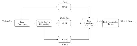
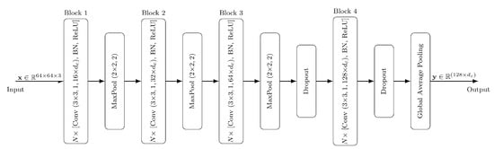
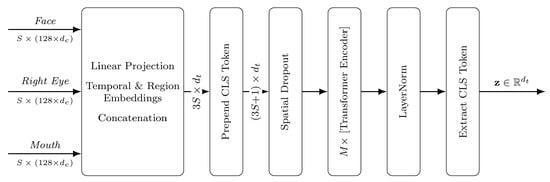
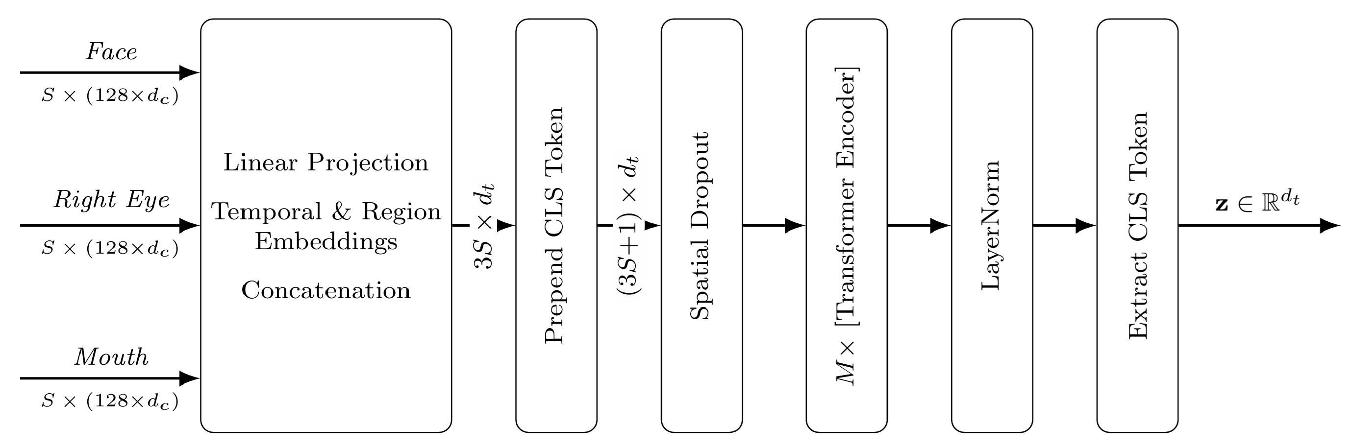
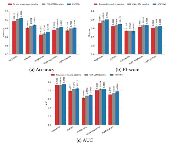
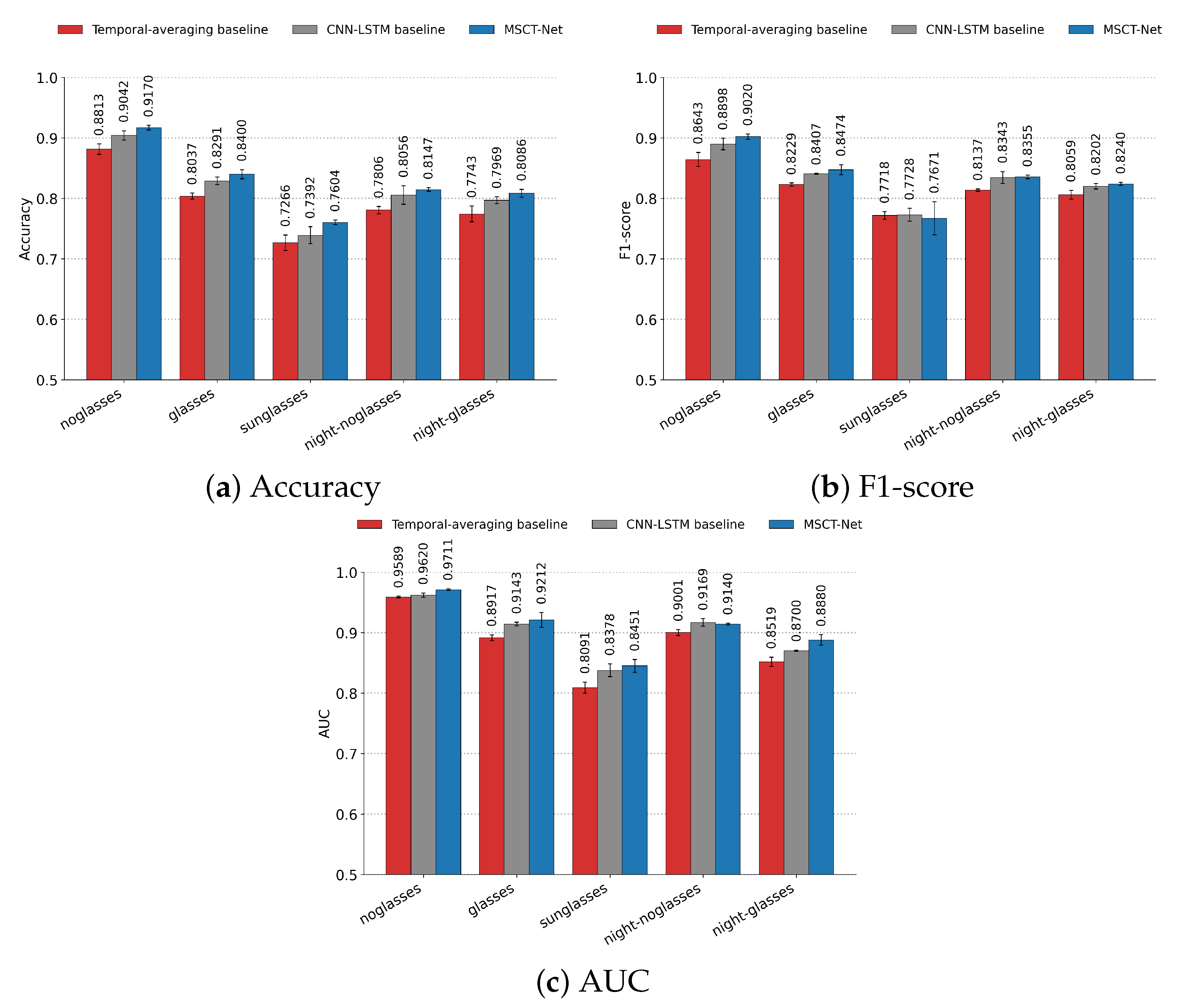
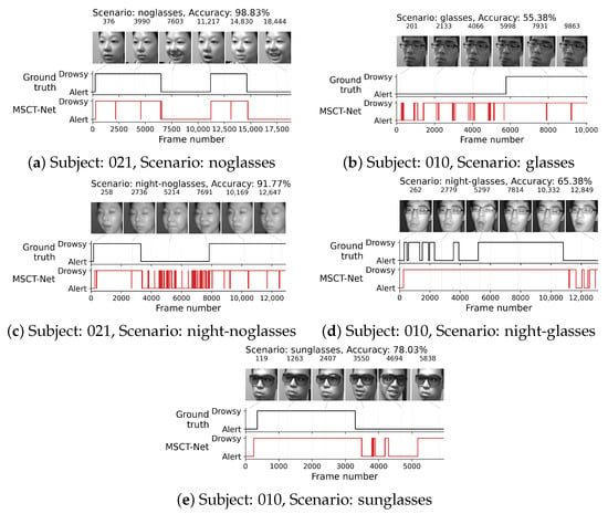
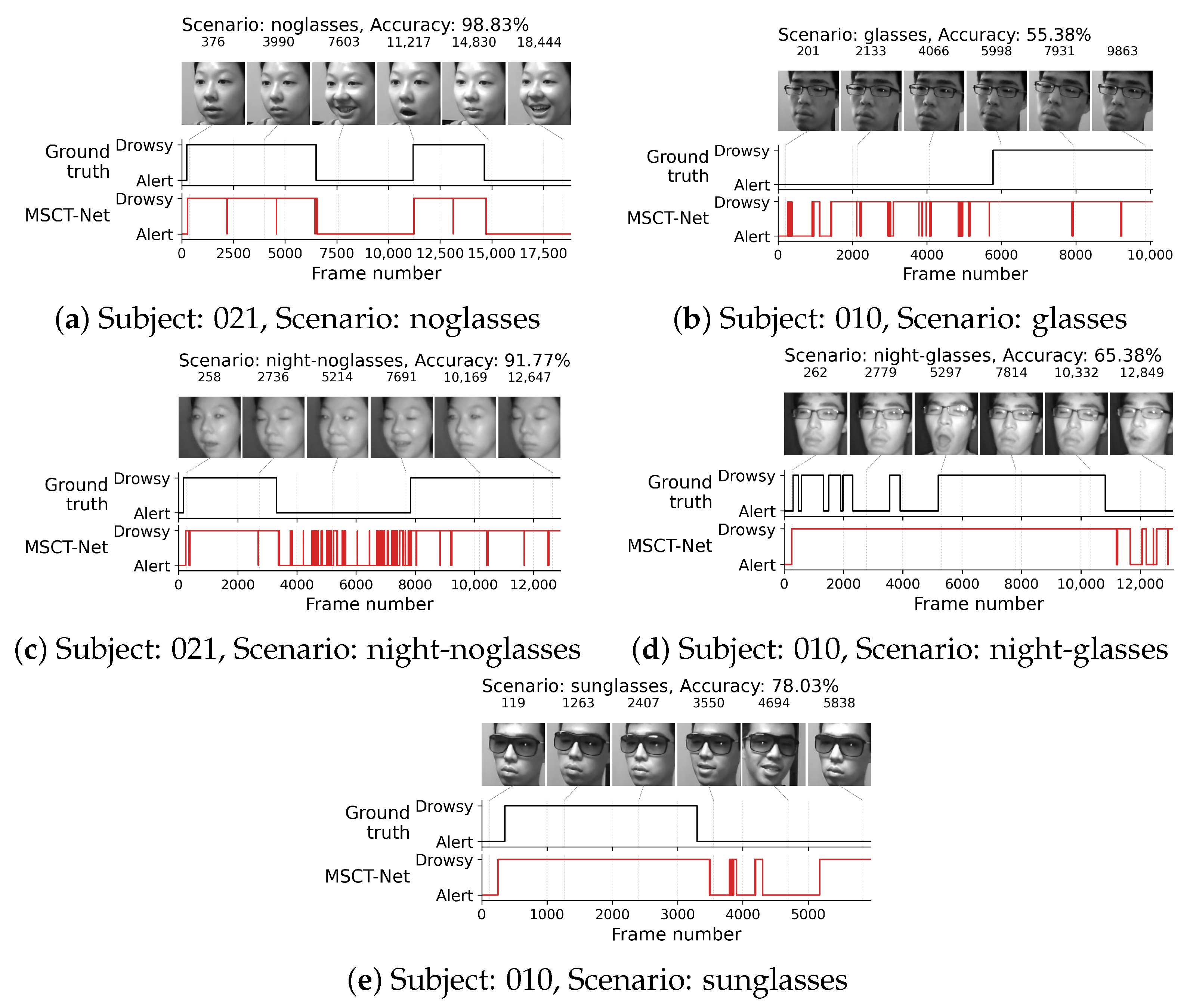
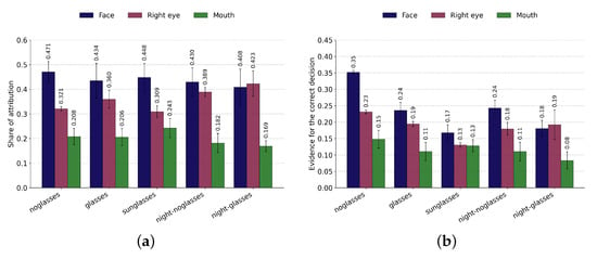
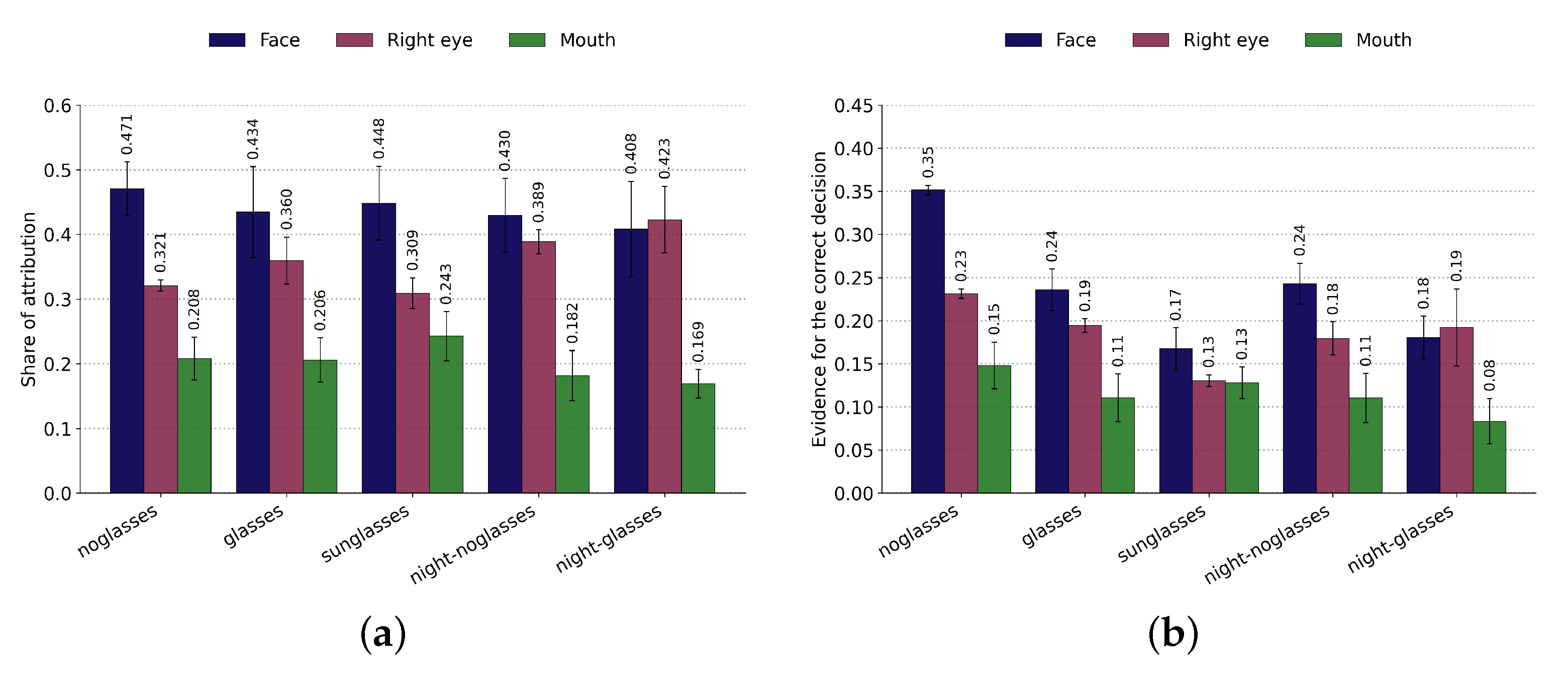

Disclaimer/Publisher’s Note: The statements, opinions and data contained in all publications are solely those of the individual author(s) and contributor(s) and not of MDPI and/or the editor(s). MDPI and/or the editor(s) disclaim responsibility for any injury to people or property resulting from any ideas, methods, instructions or products referred to in the content. |
© 2026 by the author. Licensee MDPI, Basel, Switzerland. This article is an open access article distributed under the terms and conditions of the Creative Commons Attribution (CC BY) license.