


Abstract
Strategic logistics network management requires decision support that anticipates demand and disruption uncertainty and evaluates candidate decisions before implementation. This paper presents GATrESN, a simulation-based predictive–prescriptive framework that couples Echo State Networks, a fixed parameter-free multi-head attention mechanism and a genetic algorithm over a robust scenario objective into a single decision loop over capacity, cost, inventory, workforce, resilience, and supplier redundancy. The case study is a panel of 24 sites, 16 product families, and 640 periods with 1800 matched decision instances. Against a linear-programming benchmark corrected so that the evaluator’s quality threshold is visible to it, and scored against realized rather than forecast states, the framework improves the strategic score by 0.0236 (95% bootstrap CI 0.0222–0.0250); the apparent margin against the original, weaker benchmark specification was 0.0596. Four external optimizers of the same objective reach the same operating region, and replacing the predictive core with a ridge readout changes ex post decision quality by 0.0001, locating the advantage in the robust objective rather than in the optimizer or the forecasting architecture. A closed-loop rolling-horizon experiment, in which decisions alter installed capacity, inventory, and risk at the next period, widens the advantage to 0.0315 and raises the worst-period service level from 0.52 to 0.76. Without automated exchange with a physical counterpart, the implementation is a digital model; the paper specifies the data acquisition required to close that loop.
1. Introduction
Logistics networks and supply chains operate under increasing uncertainty, driven by demand variability, resource constraints, supply disruptions, technological change, and competitive pressure. Strategic supply chain and logistics network management must therefore move beyond static planning models and adopt adaptive decision-support systems that connect operational data, predictive intelligence, and scenario-based evaluation. In distributed logistics networks, strategic decisions such as capacity expansion, cost-policy adjustment, inventory buffering, workforce flexibility, and resilience investment are interdependent, dynamic, and exposed to uncertainty. A decision that appears efficient under nominal demand may become fragile when disruptions affect capacity, labor availability, service pressure, or supplier reliability. Consequently, strategic supply chain and logistics network management requires computational frameworks capable of evaluating not only expected performance but also robustness, risk exposure, and the operational consequences of alternative managerial actions before implementation.
Digital twin research has increasingly emphasized the integration of cyber-physical data, simulation, and decision support as a mechanism for monitoring and improving operational systems [1,2]. Digital twins provide a promising mechanism for representing real or conceptual systems in a dynamic computational environment. In manufacturing and supply chain contexts, prior research has distinguished digital models, digital shadows, and digital twins according to the degree of data integration and feedback between physical and virtual systems [3]. This distinction is important for strategic logistics network management because a static model or dashboard can describe a system, but it cannot fully support adaptive strategic reasoning unless it can preserve system state, simulate future scenarios, evaluate decisions, and feed performance information back into the virtual representation.
When combined with artificial intelligence, digital twins can evolve from descriptive replicas into predictive and prescriptive decision-support platforms. In this context, an AI-driven digital twin can support strategic supply chain and logistics network management by forecasting future states, simulating strategic alternatives, detecting performance deviations, and recommending adaptive actions. It can also operate as a digital laboratory in which strategic policies are tested virtually before resources are committed in the logistics network. However, the value of such a system depends on the explicit connection between the virtual state of the logistics network, the predictive model used to estimate future operating conditions, the scenario engine used to represent uncertainty, and the prescriptive mechanism used to select strategic policies. Treating these components separately may lead to fragmented decision support: forecasting models may be accurate but non-prescriptive, optimization models may be mathematically tractable but dynamically simplified, and simulation models may be informative but computationally disconnected from adaptive policy search.
This paper addresses this methodological gap by proposing GATrESN, an AI-driven digital twin framework for strategic supply chain and logistics network management. The framework combines Echo State Networks (ESNs) for temporal operational memory, a fixed, parameter-free multi-head attention mechanism structurally inspired by Transformer-style attention for long-range dependency extraction, and genetic algorithms (GAs) for strategic decision optimization. This hybrid design is motivated by the ability of reservoir computing to model nonlinear temporal systems with efficient readout training [4,5], the ability of attention mechanisms to weight relevant sequence elements [6,7], and the suitability of evolutionary search for multi-criteria optimization problems [8]. Rather than presenting these techniques as independent modules, GATrESN embeds them in a single digital twin loop: operational states are encoded through reservoir dynamics, temporally relevant dependencies are emphasized through attention, future operating conditions are forecasted, uncertain scenarios are simulated, and strategic decisions are optimized according to service, utilization, cost, and residual-risk objectives.
The central contribution is therefore the digital twin logic that connects a virtual operational state, AI-based state forecasting, scenario simulation, prescriptive policy search, and KPI feedback into one reproducible decision-support loop. The contribution is fourfold: first, it presents a modular architecture connecting logistics network data, state representation, AI analytics, scenario simulation, and strategic decision support; second, it integrates ESNs, Transformer-style attention, and GAs into a reproducible prescriptive decision model; third, it demonstrates the framework through a simulation-based case study implemented in MATLAB R2026a (The MathWorks, Inc., Natick, MA, USA); and fourth, it reports an internal audit that locates the source of the measured advantage. That audit is central to how the present version should be read. The advantage over a linear benchmark is in strategic score once the benchmark is allowed to observe the quality threshold of the evaluator and once policies are scored against realized rather than forecast states, against the obtained under the benchmark specification of our earlier comparison (Section 4.3 and Section 4.4). Four external optimizers of the same objective reach the same operating region, and replacing the predictive core with a ridge readout changes decision quality by , so the measured value originates in the robust scenario objective rather than in the optimizer or the recurrent forecasting architecture (Section 4.7). The clearest evidence for the framework is a closed-loop rolling-horizon experiment in which decisions alter installed capacity, inventory, and risk at the next period, where the advantage widens to and the worst-period service level improves from to (Section 4.8). Finally, because no automated exchange with a physical counterpart is implemented, the system is a digital model under the established taxonomy; the term digital twin is used in this paper for the target architecture, whose data requirements are specified explicitly. By emphasizing reproducibility, explicit mathematical formulation, benchmark comparison, and the digital-laboratory role of the twin, the study aims to provide a rigorous foundation for AI-driven digital twins as strategic supply chain and logistics network management tools rather than as purely descriptive monitoring systems.
The remainder of the paper is organized as follows. Section 2 reviews the literature on digital twins, artificial intelligence, and strategic decision support. Section 3 presents the proposed GATrESN digital twin framework, including the strategic logistics network decision problem, operational data structure, digital twin representation, architecture, and computational model. Section 4 reports the experimental results in the order in which they qualify one another: the predictive accuracy of the forecasting core, the prescriptive benchmark as originally specified, its correction for an evaluator term invisible to the linear benchmark and for scoring against realized states, the analyses that isolate the contribution of the objective, the optimizer and the forecasting source, the closed-loop rolling-horizon experiment, the logistics indicators beyond the composite score, the external validation on real demand data with a sweep of the data-generating process, and the computational profile of the pipeline with its implications for deployment. Section 5 and Section 6 discuss the implications of the findings and conclude the paper, respectively. Three appendices report the data-generating process and its verification, the objective-vs-optimizer ablation, and the series-independence analysis.
2. Literature Background
2.1. Digital Twins in Supply Chain and Logistics Operations
Digital twins have been widely discussed as virtual representations of physical or logistics network systems. In supply chain and logistics operations, they enable monitoring, simulation, and decision support across production, logistics, maintenance, and service systems [1,2,9,10,11]. Digital-twin-driven manufacturing research highlights the convergence of physical product data, virtual models, and lifecycle information as a basis for improving design, manufacturing, and service processes [9,12,13,14]. Similarly, the relationship between digital twins, big data, and Industry 4.0 has been described as a key pathway for transforming manufacturing systems from isolated automation toward connected and data-intensive operational intelligence [15,16,17].
Work published in this journal has reviewed the enabling technologies that link Industry 4.0 and 5.0 to manufacturing supply chains [18], traced the path from process sensing to twinning [19], and demonstrated a cyber-physical system in which a digital twin is driven by real-time SCADA telemetry [20]; the last of these illustrates the data-acquisition architecture that the present framework would require in order to close the loop with a physical network, as discussed in Section 3.9.
The digital twin concept is particularly relevant for supply chain and logistics network management because it provides a structured way to connect state representation, system behavior, and decision feedback. A digital twin is not only a visualization layer; it can operate as a computational environment in which alternative actions are evaluated before being transferred to the real logistics network. The distinction between digital models, digital shadows, and digital twins is therefore central: a digital model may represent an asset or process, a digital shadow may update through operational data, but a digital twin implies a stronger bidirectional relationship between the system and its virtual counterpart [3]. For strategic logistics network management, this distinction implies that the virtual representation should support scenario experimentation, policy testing, and performance feedback rather than only reporting historical indicators.
In supply chains and distributed operations, digital twins have been proposed as mechanisms for improving resilience, managing disruption risk, stress-testing operational networks, and supporting decisions under uncertainty. The digital supply chain twin, for example, has been framed as a tool for disruption-risk management and resilience analysis in Industry 4.0 contexts [21,22,23,24,25]. Digital twins have also been used for scheduling and resource-allocation problems in manufacturing systems [26,27,28,29,30]. This perspective is consistent with the strategic logistics network decision problem addressed in this paper, where managerial actions must balance efficiency, service continuity, capacity utilization, and residual risk. Nevertheless, many digital twin studies remain concentrated on architecture, lifecycle integration, and operational monitoring, while the explicit integration of predictive learning and prescriptive optimization into the twin remains an open methodological challenge.
2.2. Artificial Intelligence for Strategic Decision Support
Artificial intelligence techniques, including machine learning, forecasting, anomaly detection, and optimization, can enhance strategic decisions by identifying patterns and estimating future system behavior. In supply chain and logistics network management, AI becomes especially relevant when decisions depend on temporal dependencies, nonlinear interactions, and uncertain future states [31,32,33,34]. Strategic supply chain and logistics decision problems often involve time-dependent demand, capacity restrictions, cost variation, labor availability, inventory coverage, and operational-risk exposure. These variables interact dynamically, which makes purely static planning models insufficient for adaptive decision support.
ESNs and reservoir computing are particularly relevant for temporal operational data because the recurrent reservoir maps input histories into a nonlinear state space while only the readout layer is trained [4,5,35]. Reservoir computing is rooted in the broader idea that complex recurrent dynamics can be exploited for real-time computation without requiring full recurrent-network training [36,37]. This property is attractive for strategic supply chain and logistics contexts where reproducibility, computational efficiency, and interpretable simulation workflows are important. Because the reservoir can be generated with fixed random seeds and controlled spectral properties, ESN-based models can provide a practical compromise between nonlinear temporal representation and reproducible experimentation; prior work on systematic reservoir selection and hyperparameter optimization for time-series forecasting supports this design choice by showing that spectral radius, leak rate, and reservoir size can be tuned in a principled, reproducible manner rather than by ad hoc search [38].
Attention mechanisms provide an additional layer of temporal selectivity. Attention mechanisms allow neural systems to weight the segments of an input sequence that are most relevant to the current prediction [6], while the Transformer architecture demonstrated that self-attention can represent sequence dependencies without relying entirely on recurrence [7]. Recent time-series research has extended Transformer-based models to long-sequence and multi-horizon forecasting problems [39,40]. Hybrid reservoir–Transformer architectures, which couple a fixed recurrent reservoir with an attention layer to obtain interpretable, position-aware representations of structured sequential data, provide direct precedent for combining reservoir dynamics with attention rather than treating either mechanism in isolation [41]. For a logistics network digital twin, attention can be used not as a black-box replacement for simulation but as a mechanism to emphasize the historical states most relevant to current demand, risk, utilization, and capacity decisions.
A parallel line of work questions the separation between the predictive and the prescriptive stage altogether: smart predict-then-optimize replaces the statistical loss of the forecasting model with the decision loss it induces downstream [42], and the decision-focused learning literature formalizes when training a model against the objective it will serve outperforms training it for accuracy [43]. This distinction is directly relevant here, because the predictive core of the proposed framework is trained for accuracy, while its measurable contribution, as Section 4.7 shows, resides in the objective rather than in the forecast.
Finally, evolutionary optimization is suitable when strategic decision variables must be selected under nonlinear trade-offs. Genetic algorithms and elitist evolutionary search have been widely used for complex multi-objective optimization where analytical gradients may be unavailable or insufficient [8]. Robust and data-driven optimization studies in supply chain planning further emphasize the importance of evaluating decisions under uncertainty rather than optimizing only nominal operating conditions [44,45,46,47,48]. This makes GA-based search appropriate for optimizing capacity adjustment, cost policy, resilience investment, inventory buffering, workforce flexibility, and supplier redundancy within a digital twin. When the decision-maker is averse to tail outcomes rather than to dispersion as such, coherent risk measures, and in particular the conditional value at risk, provide the formal basis for the downside terms used in the objective of this paper [49]. In a strategic logistics network context, the relevant objective is rarely a single cost-minimization criterion; instead, decision-makers must consider service level, utilization, expected cost, and risk simultaneously. Evolutionary search is therefore useful because it can explore nonconvex policy spaces and evaluate candidate strategies through simulation-based objective functions.
The integration of temporal learning, attention, and evolutionary optimization is particularly promising for AI-driven digital twins. Temporal models estimate the evolving state of the system, attention mechanisms identify which portions of the operational history are most informative, and evolutionary search evaluates alternative strategic actions under simulated uncertainty. When embedded inside a digital twin, these components can transform the twin from a passive representation into an active predictive–prescriptive environment.
2.3. Research Gap
Although digital twins and AI have been studied in operational contexts, there remains a need for integrated frameworks that explicitly connect AI-driven digital twins with strategic supply chain and logistics network management. Existing studies often emphasize digital twin architecture, lifecycle data integration, or operational monitoring, while fewer approaches integrate temporal learning, attention-based dependency extraction, and evolutionary optimization into a single reproducible strategic decision workflow. This gap is important because strategic logistics network decisions require more than accurate prediction: they require the ability to evaluate alternative actions under uncertainty and to translate predicted states into robust managerial policies.
Three limitations can be identified in the current literature. First, many digital twin studies focus on representation and monitoring rather than on prescriptive strategic decision-making. Second, many AI applications emphasize forecasting performance but do not embed the forecast inside a closed-loop decision environment. Third, optimization models often simplify the temporal and nonlinear structure of operations in order to maintain analytical tractability. The proposed GATrESN framework addresses these limitations by linking digital twin state representation, ESN-based temporal encoding, attention-based dependency weighting, Monte Carlo scenario simulation, GA-based policy search, and KPI feedback in a single reproducible workflow. In particular, the literature requires models that link predictive analytics, scenario simulation, and multi-criteria strategic evaluation while preserving the digital twin as the central organizing mechanism of the decision-support system.
3. Proposed GATrESN Digital Twin Framework
3.1. Strategic Supply Chain and Logistics Network Decision Problem and Case Study Context
The strategic logistics network decision problem addressed in this study concerns the management of a distributed logistics network in which multiple operational sites and product families must be coordinated under uncertain demand, heterogeneous capacity, variable cost structures, service-level pressure, and operational risk. In this environment, managerial decisions are not limited to forecasting future demand or selecting a single production quantity; rather, they involve the simultaneous selection of capacity-adjustment policies, cost-control actions, resilience investments, inventory buffers, workforce-flexibility actions, and supplier-redundancy levels whose effects propagate over time and interact with the current state of the logistics network. A capacity expansion may improve service reliability but increase operating cost; an aggressive cost policy may improve short-term efficiency but reduce service quality and flexibility under disruption; excessive inventory or redundancy may reduce residual risk but introduce additional operating cost; and insufficient resilience investment may leave the system vulnerable to demand shocks, labor constraints, inventory shortages, or site-specific risk events.
The case study represents a strategic logistics network responsible for delivering several product families under uncertain demand and resource conditions. The logistics network is structured as a multi-site operating system with 24 operational sites, 16 product families, and 640 sequential planning periods, producing more than 245,000 operational records before supervised lag transformation. Each site is interpreted as a semi-autonomous operational unit with its own capacity profile, cost structure, labor availability, inventory coverage, and exposure to operational risk. Each product family introduces differentiated demand patterns, volatility, and service pressure. The operational context is intentionally defined at the strategic-tactical interface: the objective is not to reproduce a single shop-floor process but to evaluate how an AI-driven digital twin can support managerial decisions that affect capacity allocation, cost policy, service reliability, inventory buffering, workforce flexibility, supplier redundancy, and resilience investment across a distributed logistics network.
Let denote the set of operational sites, the set of product families, and the set of planning periods. For each site–product–period tuple , the operational state is represented by
where is demand, is base capacity, is unit cost, is service pressure, is external operational risk, is labor availability, and is inventory coverage. Labor availability and inventory coverage are indexed by rather than because, although their systematic (non-stochastic) component varies mainly with site and period, each site–product–period record is generated from an independent stochastic draw, so realized values differ across products at fixed . The strategic decision vector for a decision instance at time t is
where is the capacity multiplier, is the cost-policy multiplier, is resilience investment, is the inventory-buffer level, is workforce flexibility, is supplier redundancy, and denotes the bounded feasible policy space. The strategic logistics network decision problem can be stated as the robust policy-selection problem:
subject to
where is the scenario-level strategic utility, is a possible future operational state generated inside the digital twin, is service level, is utilization, is expected cost, and is residual risk. Equations (3)–(5) formalize the engineering problem: the model must identify a decision vector that performs well not only for a single predicted future but across a family of plausible operating scenarios before managerial action is implemented. Figure 1 illustrates this problem conceptually, showing how demand, capacity, cost, labor, inventory, and operational-risk pressures interact and must be jointly balanced through the managerial decision vector.
Figure 1.
Strategic supply chain and logistics network management problem under uncertainty, showing interacting demand, capacity, cost, labor, inventory, and operational-risk pressures that must be balanced through managerial decisions. The diagram uses the term strategic operations management, which corresponds to the strategic logistics network management terminology used in the text; the two are equivalent in this paper.
3.2. Operational Data Structure
The operational data are organized as a longitudinal site–product–period panel. Each record corresponds to one tuple , where i identifies the operational site, p identifies the product family, and t identifies the sequential planning period. The main experimental configuration contains 24 operational sites, 16 product families, and 640 planning periods, resulting in 245,760 operational records before lag construction. This structure is sufficiently broad to represent spatial heterogeneity across sites, product-specific demand behavior, and temporal dependencies across planning periods.
The dataset contains 10 variables. Three variables define the panel index: site, product, and period. Site and product are categorical identifiers encoded as integers, whereas period is an ordered temporal index. The remaining seven variables are continuous numerical operational indicators: demand, base capacity, unit cost, service pressure, external risk, labor availability, and inventory coverage. Demand represents the requested operating load; base capacity represents available operating capability before strategic adjustment; unit cost captures the operating-cost level; service pressure measures the relationship between demand and capacity; external risk captures disruption exposure; labor availability measures workforce readiness; and inventory coverage represents buffer availability. No missing values are present in the generated computational dataset used by the model pipeline.
Figure 2 shows how the operational data are transformed into digital twin states. The raw panel is first ordered by site, product, and period. The seven continuous indicators are then converted into lagged temporal windows of length , allowing the ESN–attention layer to learn from recent operational history rather than from isolated observations. These lagged states feed the digital twin representation, where future demand and risk are forecasted and scenario-ready virtual states are created. The prescriptive stage evaluates 1800 matched decision states, each of which is solved by GATrESN and re-evaluated under the Rule-Based and LP-Simplified benchmark policies. As a result, the benchmark dataset contains 5400 rows, corresponding to the same 1800 decision states evaluated by three decision mechanisms.
Figure 2.
Organization of the operational data used by the GATrESN digital twin, from the site–product–period panel to lagged temporal states, matched decision instances, benchmark comparison, and KPI-based validation. The diagram labels the panel enterprise operations data, which is the logistics network operational panel described in the text.
Table 1 summarizes the role, type, and observed scale of each of these ten columns, namely, the three identifiers and the seven continuous indicators. This organization is important for the proposed AI-driven digital twin because it preserves the three dimensions required by the strategic logistics network decision problem: cross-site heterogeneity, product-family heterogeneity, and temporal evolution. It also supports paired model validation because all decision mechanisms are evaluated on the same digital twin states and the same KPI definitions. Therefore, differences among GATrESN, Rule-Based, and LP-Simplified policies are attributable to the prescriptive decision logic rather than to changes in data structure, state representation, or evaluation criteria.
Table 1.
Operational data structure used by the digital twin.
3.3. Data-Generating Process
The operational panel is produced by an explicit data-generating process whose functional form, parameters, and verification are reported in full in Appendix A. In summary, demand combines a site- and product-scaled trend, two seasonal components, an autoregressive disruption memory, and Gaussian noise; capacity, unit cost, labor availability, inventory coverage, and operational risk are driven by the same disruption state, so that adverse conditions co-occur across variables as they do in an operating network. Appendix A also documents the verification that the generator does not embed a structure favorable to the proposed method: no component of the generator, the predictive core, or the optimizer has access to the parameters, seeds, or memory states of the others, and all methods observe only realized values.
3.4. Digital Twin Representation and Framework Architecture
In this study, the digital twin is defined as a dynamic virtual representation of the strategic logistics network rather than as a static dataset, dashboard, or standalone forecasting model. The twin maintains a time-indexed state vector describing the relevant operating condition of the logistics network, including demand, capacity, unit cost, service pressure, labor availability, inventory coverage, and operational risk. This state representation is updated through operational observations and transformed into lagged temporal windows so that the virtual system preserves memory of prior conditions, disruption persistence, and cross-period dependencies. The digital twin layer therefore acts as the computational environment in which the logistics network can be observed, projected, stressed, and evaluated before managerial action is implemented.
The central idea is that the digital twin represents possible solutions before they occur in the real system. A candidate strategy is not adopted directly; it is first injected into the virtual logistics network, exposed to uncertain scenarios, and evaluated through the same performance logic used to assess real operations. In this sense, the twin is a digital laboratory for strategic decision-making: it creates plausible futures, tests the consequences of strategic actions, and helps decision-makers understand what may happen if the logistics network increases capacity, reduces cost, invests in resilience, expands inventory buffers, improves workforce flexibility, or adds supplier redundancy. The digital twin therefore supports anticipatory management because it turns future uncertainty into simulated evidence before the logistics network commits resources.
The proposed digital twin performs five functions. First, it represents the current and historical operational state of the logistics network at site, product, and period levels. Second, it preserves temporal memory by converting operational observations into lagged windows. Third, it predicts future operating states through the ESN–attention forecasting core. Fourth, it creates scenario-based replicas of uncertain future conditions by applying demand, capacity, cost, and risk shocks to the predicted state. Fifth, it evaluates strategic policy alternatives by computing service level, utilization, expected cost, residual risk, and composite strategic score. The feedback layer closes the digital twin loop by returning KPI information to the virtual state representation, enabling the system to support adaptive strategic learning rather than one-shot optimization.
Mathematically, the digital twin at time t is represented as
where is the observed operational history, contains structural operating parameters such as site and product characteristics, contains KPI feedback from prior evaluations, denotes the embedded GATrESN predictive–prescriptive model, and denotes the scenario-generation mechanism. The twin evaluates a candidate policy through
meaning that each policy is evaluated over a set of possible future scenarios before it is recommended.
- GATrESN Framework Architecture.
The proposed GATrESN framework is the operational structure that makes the digital twin predictive and prescriptive. It consists of six connected layers: the logistics network system layer, the data layer, the digital twin state layer, the AI analytics layer, the strategic decision layer, and the feedback layer. These layers connect operational indicators, temporal forecasting, scenario simulation, strategic optimization, and KPI-based learning. The framework is aligned with the view that digital twins should support a structured connection between physical or logistics network states, virtual representations, data analytics, and decision feedback [2,3].
Figure 3 depicts these six layers and their connections in detail. The logistics network system layer defines the real or conceptual strategic logistics network: sites, product families, planning periods, capacity structures, cost profiles, labor availability, inventory coverage, and risk exposure. The data layer transforms these indicators into structured temporal windows. The digital twin state layer stores the operational memory of the system and provides the virtual environment in which future states are projected. The AI analytics layer contains the ESN–attention predictive core, which estimates future demand and risk from temporal operational patterns. The strategic decision layer uses the predicted state as input to a GA-based optimizer that searches over policy packages. Finally, the feedback layer returns service, utilization, cost, risk, and strategic-score indicators to the digital twin state, closing the loop between virtual experimentation and adaptive strategic learning.
Figure 3.
Detailed architecture of the proposed GATrESN AI-driven digital twin framework, integrating logistics network operations data, digital twin state representation, temporal feature engineering, ESN–attention forecasting, scenario simulation, GA-based prescriptive optimization, and KPI feedback. The blocks labeled with operations-management terms inside the diagram, in particular strategic operations management and enterprise operations data, denote the strategic logistics network management layer and the logistics network operational panel described in the text; the terms are equivalent in this paper. The diagram depicts the target architecture, in which the loop is closed on live operational data; Section 3.9 states which of its elements the present implementation realizes.
This architecture is intentionally hybrid. The ESN is used because strategic logistics network data are temporal and nonlinear; attention is used because not all historical states are equally relevant to the next strategic decision; and the GA is used because the decision space is nonlinear, bounded, multi-criteria, and difficult to solve through a single closed-form optimization model. The result is not simply a combination of three algorithms but a digital twin workflow in which temporal learning, scenario generation, and policy optimization are coupled around the same virtual representation of the logistics network.
3.5. GATrESN Computational Model
The GATrESN computational model is the core methodological contribution of this paper. It defines how the AI-driven digital twin converts an observed operational history into a recommended strategic policy. The model is built as a predictive–prescriptive chain. First, the ESN maps lagged operational states into nonlinear reservoir trajectories that preserve temporal memory. Second, a fixed, parameter-free multi-head attention operator assigns relevance weights to the reservoir trajectory so that the model can emphasize the historical states that matter most for the current decision, without introducing any additional trainable parameters. Third, a ridge readout converts the ESN–attention representation into forecasts of future demand and risk. Fourth, the digital twin generates possible future scenarios around those forecasts. Fifth, the GA searches for the strategic decision vector that maximizes robust utility across those scenarios.
GATrESN combines three computational components inside the digital twin. First, an ESN encodes nonlinear temporal dynamics through reservoir states. ESNs are a form of reservoir computing in which a fixed recurrent reservoir transforms input sequences into high-dimensional dynamic states, while a comparatively simple readout is trained for prediction [4,5]. Second, a fixed, parameter-free multi-head dot-product attention mechanism, structurally inspired by Transformer-style attention [6,7] but without trainable query/key/value projections, extracts long-range dependencies from lagged reservoir representations by weighting each historical reservoir state according to its similarity to the current state within fixed reservoir sub-blocks (Equations (9)–(11)). Third, a GA optimizes strategic decision variables within the digital twin, including capacity adjustment, cost policy, resilience investment, inventory buffering, workforce flexibility, and supplier redundancy, following the use of evolutionary search for complex nonlinear optimization problems [8]. The AI components therefore operate as the predictive and prescriptive engines of the twin, while the digital twin provides the stateful environment in which forecasts, scenarios, decisions, and feedback are consistently evaluated.
The mathematical foundation of GATrESN is defined as a sequential predictive–prescriptive mapping that links digital twin state representation, reservoir-based temporal encoding, attention-based dependency weighting, scenario simulation, and evolutionary policy optimization. Let denote the aggregated operational state vector of the digital twin at time t. For a lag length L, the digital twin observes the temporal window . The ESN component maps this window into nonlinear reservoir states according to
where is the reservoir state, is the leak rate, is the input matrix, and is the recurrent reservoir matrix scaled to satisfy the echo-state stability condition through a controlled spectral radius . The resulting reservoir trajectory is then processed by a fixed, parameter-free multi-head dot-product attention operator, structurally inspired by Transformer-style attention [7] but without trainable query, key, or value projections. The -dimensional reservoir state is partitioned into M contiguous, non-overlapping blocks of size using fixed binary selection matrices , , which are set once by construction (from the reservoir indexing) and are not updated during training. For head m, the query is the corresponding block of the current reservoir state, and the key and value are identical and equal to the same block evaluated across the lagged context window:
so that , and ; no separate value transformation is applied, and the query/key/value roles are realized entirely through the fixed block-selection operator rather than through learned matrices , , . The attended representation for head m is
where the softmax is taken over the L time steps of the context window, yielding a scalar attention weight per lagged reservoir state and an attended vector . Each head is then collapsed to a single scalar by mean-pooling over its components, , and the complete attention vector is the concatenation of the M pooled scalars:
With the reservoir size and heads used throughout this study, each head spans reservoir units and . Because is fixed and there is no value projection, this attention layer has zero trainable parameters of its own; it is not optimized by backpropagation or by any other gradient-based procedure. The only learned parameters in the entire predictive core are the readout weights in Equation (12), fit in closed form by ridge regression (Section 3.6), given the fixed reservoir (, , drawn once at initialization and never updated) and the fixed attention operator described above. Section 5 returns to the implications of this design choice, and the predictive-only ablation reported in Section 4.1 quantifies its effect on forecasting accuracy relative to a reservoir without attention and to a linear baseline.
The predictive layer combines the lagged operational window, the final ESN state, and the attention representation to estimate the next-period demand and risk state:
The readout matrix is estimated through ridge regression to maintain numerical stability and reproducibility:
where is the matrix of training feature vectors, is the target matrix, and is the regularization coefficient.
The prescriptive layer uses the strategic decision vector defined in Equation (2). For each Monte Carlo scenario , the digital twin transforms the predicted demand and risk into shocked states and . Given base capacity and unit cost , the scenario-dependent effective capacity is
where , , and represent the capacity-equivalent effects of workforce flexibility, inventory buffering, and supplier redundancy. The quality effect of aggressive cost reduction is represented by
The scenario-level service, utilization, cost, and residual-risk indicators are then defined as
where clips values to the interval ; the variable-cost term in Equation (18) is charged on , the quantity actually fulfilled (Equation (16)), rather than on gross forecasted demand, so that unfulfilled demand is not billed; , , , , and are policy cost coefficients, and , , , and are risk-mitigation coefficients.
For each scenario, the strategic utility of a candidate policy is computed as
where is the target utilization, is normalized cost, is a minimum acceptable service-level threshold below which a linear shortfall penalty is applied, is a reference policy used to discourage extreme or operationally unstable decisions via the mean absolute deviation , and , , , , , and are scalar weights. The robust objective optimized by the GA is
Here, denotes the pth percentile of the scenario distribution of , is a minimum acceptable 10th-percentile utility threshold, the third term penalizes a low 10th-percentile outcome relative to , the fourth term penalizes a wide gap between the scenario mean and the 5th-percentile tail (an empirical downside-tail-width penalty), and , , and control risk aversion to dispersion, 10th-percentile downside performance, and tail width, respectively. Therefore, the complete GATrESN mapping can be summarized as
where denotes reservoir temporal encoding, denotes attention-based temporal dependency extraction, denotes the ridge readout, denotes Monte Carlo scenario simulation, and denotes genetic-algorithm-based prescriptive optimization. This formulation makes explicit that GATrESN is not a simple ensemble of three independent techniques but a coupled predictive–prescriptive digital twin in which the ESN and attention components estimate the future operational state and the GA searches for robust strategic policies conditional on that learned state.
Operationally, Equation (22) means that the model does not optimize a strategy from raw data directly. It first reconstructs the temporal state of the logistics network, identifies the most informative historical dependencies, forecasts the future demand–risk condition, expands that forecast into multiple plausible scenarios, and only then searches for a robust strategic policy. This sequence is essential for strategic logistics network management because it separates the question of what the logistics network is likely to face from the question of what action should be taken under uncertainty. GATrESN therefore acts as a decision engine embedded inside the digital twin: the ESN provides memory, attention provides temporal selectivity, scenario simulation provides uncertainty exposure, and the GA provides prescriptive search.
After a candidate policy is evaluated, the digital twin state is updated through a feedback operator:
where is the KPI vector generated by the scenario evaluation, whose components are the service level, utilization, expected cost, residual risk, and strategic score defined in Section 3.5. Equation (23) formalizes the digital twin character of the framework: the model maintains a virtual state, uses AI to project that state, tests actions in simulated future conditions, and feeds the resulting performance indicators back into the twin representation.
3.6. Reproducibility
Reproducibility in this study is established through the explicit disclosure of the computational structure, model configuration, source-code workflow, generated data structure, and experimental outputs. The complete MATLAB implementation generates the logistics network operations dataset, constructs the lagged digital twin state, trains the ESN–attention predictive layer, executes the GA-based prescriptive layer, evaluates benchmark policies, exports numerical results, and produces all figures used in the manuscript. Therefore, the reported results are not produced by manual post-processing; they are generated by a single reproducible computational pipeline.
The operational panel comprises 384 site–product series, each contributing 628 consecutive lagged observations after the 12-period lag window is applied, for n = 241,152 supervised rows in total. Rows are laid out series-by-series, in chronological order within each series, and the 70/15/15 train/validation/test partition is then applied as a fixed cut on this concatenated row index (, ) rather than as a chronological cutoff shared across all series. Because every series contributes the same number of rows, this row-index cut coincides almost exactly with series boundaries: 382 of the 384 series fall entirely within a single partition (268 in training, 57 in validation, 57 in testing), and the two partition boundaries each split exactly one series across the adjacent partitions, namely, series 269 across train/validation (rows 1–502 in training, rows 503–628 in validation) and series 327 across validation/test (rows 1–251 in validation, rows 252–628 in testing). Neither of these two split series contributes rows to both training and testing; the straddling is confined to the train/validation and validation/test boundaries. This yields 269 series (168,806 rows, 70.0%) touching training (268 exclusively, plus the first 502 rows of series 269), 59 series (36,173 rows, 15.0%) touching validation (57 exclusively, plus series 269 and 327 partially), and 58 series (36,173 rows, 15.0%) touching testing (57 exclusively, plus the final 377 rows of series 327), where series 269 and 327 are each counted in both of the two adjacent partitions they straddle; the totals therefore sum to , not 384, precisely because of this double-counting. Consequently, the test-set forecasting metrics reported in Section 4.1 measure generalization to site–product series that never appeared in training, namely, 57 series held out entirely, plus the final 377 rows of series 327, whose only prior appearance was in validation, not training, rather than to later periods of series already observed during training. Feature normalization (z-scoring) statistics (, ) are computed exclusively from the training partition and then applied to the validation and test partitions, preventing validation/test statistics from leaking into the normalization step. The 1800 strategic decision instances used for the prescriptive benchmark and SHAP analyses are drawn from the test partition using stratified sampling across all 58 test-partition series, rather than from a contiguous block of test rows, so that the reported benchmark and explainability results reflect the full held-out operational diversity rather than a small subset of series. Because rows from different site–product series are concatenated series-by-series into each partition, a series-boundary group identifier is tracked for every row (one integer per site–product pair), and both the ESN reservoir state in Equation (8) and the lagged attention context window in Equation (9) are reset whenever this identifier changes between consecutive rows: the reservoir state is reinitialized to zero at the first row of every series, and the attention context is clipped so it never extends past the most recent series boundary. This guarantees that no reservoir state or attention weight ever propagates across the boundary between two unrelated site–product series.
The experimental configuration used for the reported results includes 24 operational sites, 16 product families, 640 planning periods, 12 temporal lags, 240 ESN reservoir units, a spectral radius of 0.92, 8 attention heads, 1800 strategic decision instances, 35 Monte Carlo scenarios per decision instance, a GA population size of 140, and 180 GA generations. The random seed was fixed at 2026, and deterministic seeds were assigned to each decision instance so that the stochastic elements of data generation, reservoir initialization, scenario simulation, and GA search can be reproduced. Parallel execution was enabled through MATLAB parfor, using 12 requested workers on a Mac mini M4 Pro with 12 CPU cores. The parallelization affects execution time but not the mathematical definition of the model, because decision instances are independently seeded and evaluated under the same objective function.
The reproducibility protocol can be summarized as
where denotes the MATLAB source code, denotes the generated logistics network operations dataset, denotes the ESN–attention configuration, denotes the genetic-search configuration, denotes the scenario-simulation configuration, and denotes the exported tables, figures, benchmark results, and reproducibility metadata. This structure allows the experiment to be replicated by rerunning the same code rather than by reconstructing the model from narrative description alone.
3.7. Experimental Design: Benchmark Models and Extended Comparison
To evaluate whether the proposed GATrESN decision layer provides value beyond established decision mechanisms, the same case study is compared against two benchmark models: LP-Simplified and Rule-Based. These two policies define the primary comparison reported throughout Section 4; an extended set of external predictive and prescriptive methods is specified separately in Section 3.8 and evaluated in Section 4.6. These benchmarks were selected because deterministic optimization and threshold-based managerial policies are widely used in operations planning, capacity management, inventory control, and risk-response decision-making. The objective is therefore not to compare GATrESN against arbitrary alternatives but to evaluate whether the proposed AI-driven digital twin improves upon two common classes of strategic logistics decision models: analytical planning models and managerial heuristic policies.
The first benchmark, LP-Simplified, represents a deterministic linear programming approximation of the strategic logistics network decision problem. It minimizes a linear operating-cost function over the same six decision variables used by GATrESN:
subject to linearized service and risk constraints:
Here, contains the linearized cost coefficients associated with capacity adjustment, cost policy, resilience investment, inventory buffering, workforce flexibility, and supplier redundancy. This benchmark captures the logic of conventional deterministic planning: it is computationally efficient and interpretable, but it simplifies nonlinear interactions, downside uncertainty, and scenario-dependent trade-offs.
The second benchmark, Rule-Based, represents a structured managerial heuristic. It uses demand pressure and forecast risk as decision triggers:
where is the forecasted demand-pressure index. The policy is defined by threshold rules:
The high-risk policy increases resilience investment, inventory buffering, workforce flexibility, and supplier redundancy. In all three branches, the capacity multiplier is set by the same continuous rule, , so it responds to demand pressure rather than to the branch, which is why it is reported as a formula rather than as a constant in Table 2. The linearized cost vector of the LP benchmark is , and the service-constraint coefficients are , , and , with risk-constraint coefficients , , and ; Section 4.3 shows that the lower bound on in this formulation, not these coefficients, is what determines the benchmark’s measured performance. The pressure policy increases capacity and operational flexibility when forecasted demand exceeds available capacity. The base policy applies conservative adjustments under normal operating conditions. This benchmark reflects how many organizations operationalize strategic decisions through expert rules, risk thresholds, and demand-pressure triggers when full stochastic optimization is unavailable or impractical.
Table 2.
Experimental and decision-model parameters. All values are fixed configuration constants of the reproducible MATLAB pipeline (Section 3.6); none are fitted or tuned per decision instance.
Both benchmarks use the same forecasted demand, forecasted risk, base capacity, and unit-cost inputs as GATrESN. They are also evaluated using the same digital twin performance indicators: service level, utilization, expected cost, residual risk, and composite strategic score. The comparison therefore isolates the prescriptive decision mechanism rather than changing the data, forecasts, case-study structure, or performance metrics. Under this design, differences in results can be attributed to how each model converts the same digital twin state into a strategic policy.
3.8. Experimental and Decision-Model Parameters
Equations (8)–(21) introduce a substantial number of fixed constants that govern the predictive core, the effective-capacity and quality-penalty terms, the cost and risk functions, the scenario-utility weights, and the robust GA objective. All of these values are configuration constants of the single reproducible MATLAB pipeline (Section 3.6); none are fitted, tuned per instance, or learned from data. Table 2 reports the exact numerical value of every such constant, organized by the equation and layer in which it appears, so that the model is fully specified independently of the source code.
- Extended benchmark configuration.
To establish that the performance reported below is a property of the proposed decision formulation rather than of a narrow comparison set, the benchmark is extended in both layers of the framework. Every added method is evaluated on the same digital twin states, the same held-out partition, the same 1800 matched decision instances, and in the prescriptive layer, the same Monte Carlo scenario set per instance, so that all comparisons remain paired at the level of the individual decision.
Five additional decision methods operate on the identical decision vector of Equation (2) and the identical robust objective of Equation (21): (i) a replicated genetic algorithm with the configuration of Section 3.8 (population 140, 180 generations, mutation rate 0.12), which serves as a control for the re-implementation; (ii) particle swarm optimization with 140 particles and 180 iterations, inertia decreasing linearly from 0.9 to 0.4 and cognitive and social coefficients of 1.5; (iii) simulated annealing with 20 parallel chains of 1260 steps, matching the genetic algorithm’s budget of 25,200 objective evaluations, under a quadratic cooling schedule; (iv) a sample-average-approximation policy that maximizes the expected scenario utility of Equation (20) instead of the robust objective, searched with the same genetic operator so that only the objective differs; and (v) a policy that maximizes the conditional value at risk of the scenario utility, approximated by the mean of the two worst of the 35 scenarios. Methods (iv) and (v) isolate the contribution of the risk-aware terms of the objective, whereas (ii) and (iii) isolate the contribution of the search mechanism itself.
Four additional forecasting models are trained on the supervised panel of Section 3.6. Two are global models that follow the GATrESN protocol, fitted on the training series and evaluated on the held-out series: histogram-based gradient-boosted regression trees (400 boosting iterations, learning rate 0.08, early stopping) and a two-layer GRU network (64 hidden units, Adam optimizer, batch size 512, early stopping on the validation partition, five random seeds). Two are classical per-series models fitted on each held-out series’ own early history and evaluated one step ahead over its later periods: a seasonal ARIMA model and an additive Holt–Winters model with damped trend and seasonal period 12. Because the per-series models consume part of each held-out series for estimation, their metrics are reported on the common evaluation subset formed by the later of every held-out series, and the global models are reported on both scopes so that the comparison is like for like.
The additional baselines were implemented in Python 3.11.15 (NumPy 2.4.6, scikit-learn 1.9.0, statsmodels 0.14.6, PyTorch 2.14.0) on top of a port of the decision model of Section 3.5, and the port was validated before any new result was produced. Re-evaluating the stored decision vectors of the three original methods reproduces all 5400 published benchmark rows with a maximum absolute deviation of on expected cost and machine precision on the remaining indicators, and the reconstructed supervised panel reproduces the persistence and linear/ridge baselines of the predictive ablation reported in Section 4.1 to within . Because the Gaussian random streams of the two environments cannot be made bit-identical, the Monte Carlo scenario sets were regenerated once per decision instance and shared by all optimizers, including the replicated genetic algorithm; the difference between the originally reported result and that replication therefore quantifies the effect of the scenario realization and is reported in Section 4.6.
3.9. Data Acquisition, Feedback Loop, and Position in the Digital Twin Taxonomy
Two questions must be answered before the framework can be called a digital twin: what data would drive it in an operating network, and how tightly the virtual and physical systems are coupled. We answer both explicitly, and we place the present implementation where the evidence puts it rather than where the terminology is most favorable.
What the twin consumes. The virtual state of Equation (1) is built from a site–product–period table with seven fields: realized demand, available capacity, unit operating cost, labor availability, inventory coverage, and the derived service pressure and operational risk. In a deployment, these originate in systems that most logistics organizations already operate: order and shipment lines from the enterprise resource planning system supply demand; warehouse and transport management systems supply throughput, available capacity, and inventory positions; the human-resources or shift-planning system supplies labor availability; and procurement records supply unit costs and supplier status. Risk is not an input but a derived indicator, computed from labor and inventory shortfalls and from disruption signals. Where telemetry exists—gate scans, vehicle position, conveyor or AGV utilization, and temperature and condition sensors on sensitive freight—it enters the same state vector as higher-frequency measurements of capacity and service pressure, which is the architecture demonstrated for SCADA-driven twins in cyber-physical installations [20] and the progression from process sensing to twinning described for manufacturing processes [19].
Refresh and feedback. The twelve-period lag window sets the minimum history: a site–product series becomes usable after thirteen observed periods. The offline component of the pipeline—state reconstruction, reservoir states, attention features, and readout estimation—is refreshed when new periods close, whereas the decision stage is re-run whenever the forecast or the managerial preference weights change (Section 4.13). The feedback path implemented in this paper is closed within the simulation: in the rolling-horizon experiment of Section 4.8, the decision taken at one period alters installed capacity, inventory, and risk at the next, and those altered states are what the twin observes when it decides again. The path that remains open is the physical one: no measurement from an operating network enters the state, and no recommendation leaves it.
Where this places the system. Under the taxonomy that distinguishes digital models, digital shadows, and digital twins by the direction and automation of data flow [3], an implementation without automated data exchange with a physical counterpart is a digital model, not a digital twin, regardless of how faithfully it represents system dynamics. We therefore describe the contribution of this paper as a simulation-based predictive–prescriptive framework with a closed decision loop, which is what the experiments support. The term digital twin is retained only for the target architecture—the same loop instantiated on live operational data—and the requirements for reaching it are the data sources listed above, an automated ingestion path, and the governance that must precede acting on a prescriptive recommendation.
4. Results
This section reports the predictive and prescriptive performance obtained from the reproducible experimental protocol, organized so that each result is immediately followed by the analysis that qualifies it. Section 4.1 establishes the accuracy of the forecasting core across partitions. Section 4.2 reports the prescriptive comparison as it was originally specified, and Section 4.3 and Section 4.4 correct that comparison on its two substantive weaknesses, an evaluator term the linear benchmark could not observe and a scoring convention based on the model’s own forecasts; the corrected figures supersede those of Section 4.2, which is retained because the earlier version of this work reported them. Section 4.6 and Section 4.7 then isolate where the surviving advantage originates, by varying the optimizer, the objective, and the forecasting source independently. Section 4.8 evaluates the policies when decisions alter subsequent states, Section 4.9 reports indicators beyond the composite score, and Section 4.10, Section 4.11, Section 4.12 and Section 4.13 report external validation, robustness across data-generating regimes, managerial preference scenarios, explainability, and computational cost. To keep the magnitudes unambiguous, the strategic-score advantage over the linear benchmark is reported throughout as a chain: against the originally specified benchmark, against the quality-aware benchmark, when additionally scored against realized states, and in the closed loop. All prescriptive comparisons use the same 1800 matched decision instances, in which every policy receives the same forecasted demand, forecasted risk, base capacity, unit cost, and KPI definitions.
4.1. Predictive Performance of the Forecasting Core
The forecasting results in Table 3 indicate stable generalization across the training, validation, and test partitions for both predicted variables. For demand, RMSE increases from in training to in testing (MAE from 8.868 to 9.296), while decreases modestly from 0.786 to 0.755; this small degradation suggests that the ESN–attention predictive core did not simply memorize the training sequence but retained enough temporal structure to explain three-quarters of the demand variance in unseen series. For external risk, absolute errors are small in native units (RMSE , MAE , consistent with a variable bounded in ), but is substantially lower and declines from 0.191 in training to 0.120 in testing, indicating that the reservoir–attention core explains only a limited share of risk variance beyond what a constant-mean predictor would achieve; risk is evidently harder to forecast from the available lagged operational state than demand is. We report both variables separately, rather than a single pooled error, precisely because their native scales differ by more than two orders of magnitude and a joint metric in original units would be driven almost entirely by the demand component. In the proposed framework, forecasting accuracy is still relevant to the prescriptive layer because the predicted demand–risk pair is used as the input condition for scenario simulation and policy search regardless of its absolute precision, but the weaker risk-forecasting fidelity should be read as a limitation of the predictive core discussed further in Section 5. As detailed in Section 3.6, the partitions are formed by holding out site–product series rather than by cutting the panel chronologically: 382 of the 384 series fall entirely within one partition, with only two series split across an adjacent partition boundary as a residual effect of the row-index cut; the small train-to-test increase in error therefore reflects generalization to previously unseen operational series, not merely to later time periods of already-observed series.
Table 3.
Forecasting performance of the GATrESN predictive core, reported separately per output variable. The readout jointly predicts (Equation (12)); demand and risk are evaluated on their native scales because demand ranges approximately 17–214 while external risk is bounded in , so a single pooled RMSE/MAE in original units would be dominated by the demand component alone. Values are means ± standard deviations over 15 random initializations of the reservoir and of the attention projections, on the same partitions; the previously submitted version of this table reported a single initialization, whose test demand RMSE of 12.021 lies at the 87th percentile of the seed distribution reported here, and is consistent with the aggregate value reported in Section 4.6.
The results in Table 3 report the full GATrESN predictive core, but they do not by themselves establish that its ESN–attention design is necessary: the benchmark comparison of Section 4.2 evaluates only prescriptive policies (LP-Simplified, Rule-Based) downstream of a fixed forecast, so it cannot attribute strategic gains to the predictive architecture. To isolate the contribution of the reservoir and the attention layer to forecasting accuracy itself, Table 4 reports a predictive-only ablation on the test partition, comparing four models of increasing complexity under the same ridge-regularized readout and the same 12-lag input window: a persistence (naive) forecast that carries forward the most recent observed demand and risk value; a linear ridge regression on the raw lagged features, with no reservoir or attention; the ESN reservoir with the raw lagged features but without the attention layer; and the full GATrESN predictive core.
Table 4.
Predictive-only ablation on the test partition, isolating the contribution of the ESN reservoir and the attention layer to forecasting accuracy (independent of the downstream prescriptive comparison in Table 5). The ESN and GATrESN rows report the mean ± standard deviation over 15 independent random reservoir draws (, ), since a single draw is not representative of the reservoir’s variability; persistence and linear/ridge involve no random initialization.
Table 4 shows that the largest gain comes from adding multivariate lagged structure at all: moving from persistence to linear ridge regression reduces demand RMSE by 18.8% and risk RMSE by 25.7% on the test partition, confirming that the lagged operational state is genuinely informative rather than trivially forecastable. Adding the ESN reservoir on top of the same raw lagged inputs, without attention, leaves demand and risk RMSE statistically indistinguishable from linear ridge (12.042 ± 0.014 vs. 12.033 for demand; 0.1490 ± 0.0004 vs. 0.148 for risk); the nonlinear reservoir alone does not improve on a linear baseline for this case-study configuration. The attention layer contributes a small but statistically reliable additional reduction relative to the reservoir-only variant, evaluated pairwise across the same 15 reservoir draws: demand RMSE falls by 1.14% ± 0.33% (paired , ), and risk RMSE falls by 0.27% ± 0.18% (paired , ). The effect is consistent in direction across every draw but modest in magnitude: with the head configuration used throughout this study (, grouping the 240-unit reservoir into eight 30-unit blocks), the full ESN–attention core does not substantially outperform a linear ridge model on pure forecasting accuracy.
This finding motivated a further sensitivity analysis, varying the number of attention heads from to (one head per reservoir unit) while holding the reservoir size, lag window, and ridge penalty fixed and averaging over 8 independent reservoir draws per head count (Figure 4). Demand RMSE decreases monotonically as H increases, reaching 11.405 ± 0.041 at , a 5.2% reduction relative to linear ridge, compared to the 1.1% reduction obtained at ; risk RMSE is comparatively insensitive to H, declining only from 0.1491 at to 0.1480 at . This confirms that the attention mechanism does carry predictive value that scales with head granularity and that is a conservative operating point rather than a ceiling on what attention can contribute. Because that sensitivity curve is computed on the test partition, it cannot by itself justify the choice of H. We therefore repeated the comparison on the validation partition only, over five independent reservoir draws per head count, obtaining a demand RMSE of for , for , for , for , and for . The validation partition therefore favors over the configuration adopted here, by a margin of , which is approximately one and a half times the seed-to-seed dispersion at either setting. The selection of H is made on this validation evidence, and no test-partition value is used for it. We retain for all reported results in this paper because it keeps the computational cost of the attention feature extraction low while capturing a meaningful share of the head-count benefit, without a corresponding change in the downstream prescriptive comparison, which depends on the forecasted demand–risk pair rather than on marginal reductions in its RMSE. We report this sensitivity analysis explicitly, rather than silently fixing , because it directly addresses whether the ESN–attention combination is justified: it is, in the sense that attention improves forecasting accuracy monotonically with head count, but the specific configuration adopted here trades a larger share of that improvement for reproducibility and computational efficiency, consistent with the design goals stated in Section 3.6.
Figure 4.
Sensitivity of test-set forecasting RMSE to the number of attention heads , , with the reservoir size, lag window, and ridge penalty held fixed. (Left) demand RMSE decreases monotonically with H; (Right) risk RMSE is comparatively insensitive to H. The dashed line marks the linear/ridge test RMSE from Table 4; the dotted line marks , the configuration used throughout this study.
4.2. Benchmark Comparison Under the Originally Specified Benchmarks
Table 5 shows that GATrESN achieved the highest composite strategic score among the evaluated decision models. Relative to the Rule-Based benchmark, GATrESN improved the mean strategic score by 9.23%, increased mean service level by 12.90%, and reduced mean residual risk by 64.79%. Relative to LP-Simplified as originally specified, GATrESN improved the mean strategic score by 7.85%, increased mean service level by 26.75%, and reduced mean residual risk by 63.91%. These figures are reported here only to document the comparison made in the previous version of this work; Section 4.3 shows that most of the service and risk differences are produced by an evaluator term invisible to that benchmark, and the corrected comparison supersedes them. These gains were obtained at the expense of higher expected cost, which increased by 14.82% relative to Rule-Based and by 53.63% relative to LP-Simplified. This cost increase should not be interpreted as inefficiency alone; it reflects a strategic policy that invests in resilience, buffers, workforce flexibility, supplier redundancy, and capacity protection to reduce downside exposure under uncertainty. That interpretation is nevertheless only partially supported: Section 4.9 shows that once cost is normalized by the units actually delivered, GATrESN is the most expensive of the defensible policies, and its case rests on an expected interruption cost three times lower rather than on cost efficiency. Consistent with the paired statistical validation in Table 6, the strategic-score improvement is itself large in effect-size terms, not only a byproduct of the service-level and residual-risk components: GATrESN’s composite-score advantage is statistically comparable in magnitude to its advantage on the individual KPIs, rather than a small residual after cost is netted out.
Table 5.
Benchmark comparison of strategic decision models under the benchmark specification used in the earlier version of this comparison. Table 7 reports the same comparison against a quality-aware linear benchmark and supersedes the service and risk differences shown here.
Figure 5 summarizes the main KPI trade-offs. GATrESN dominates the two benchmarks in service level, residual risk, and composite strategic score as those benchmarks were originally specified; Section 4.3 shows that the service and risk components of this dominance largely disappear once the linear benchmark is allowed to observe the quality threshold, and Section 4.9 shows that no dominance survives on cost per delivered unit. Rule-Based achieves the highest mean utilization, but this occurs together with higher residual risk and lower service reliability, indicating that high utilization is partly obtained by operating closer to capacity pressure. LP-Simplified achieves the lowest expected cost, as expected from its linear cost-minimization structure, but it produces the lowest service level and does not reduce residual risk as effectively as GATrESN. Therefore, the comparison shows that the proposed method is not merely optimizing a single KPI; it shifts the policy balance toward robustness and service continuity.
Figure 5.
Benchmark KPI dashboard comparing GATrESN, Rule-Based, and LP-Simplified policies using the same digital twin performance indicators. The value labels of this figure were regenerated directly from the result file: in the previously submitted version, the labels of LP-Simplified and Rule-Based were interchanged in all four panels, although the bars themselves were correct.
Figure 6 provides a distributional view of the same comparison. GATrESN shows a strategic-score distribution with a median of 0.821 and a 5th–95th percentile interval of 0.802–0.832, which no longer overlaps with either benchmark: Rule-Based (median 0.751, interval 0.705–0.794) and LP-Simplified (median 0.762, interval 0.746–0.771) both fall entirely below GATrESN’s 5th-percentile floor. Consistent with the large paired effect sizes reported in Table 6, the strategic-score distributions are as clearly separated as the other two KPIs, not closer together. The service-level distribution also shows a clear separation: GATrESN maintains near-complete fulfillment for most decision instances (median 1.000, 5th percentile 0.974), whereas Rule-Based exhibits a broader, lower range (median 0.896, 5th percentile 0.738), and LP-Simplified remains capped by the linearized service approximation (median 0.784, tightly concentrated between 0.758 and 0.820). In residual risk, GATrESN is concentrated around markedly lower values, with a median of 0.066 and a 95th percentile of 0.107, compared with a median of 0.180 (95th percentile 0.281) for Rule-Based and a median of 0.183 (tightly concentrated between 0.169 and 0.187) for LP-Simplified. These results indicate that the proposed model’s advantage is not confined to service reliability and downside risk exposure: it extends to a clean, non-overlapping margin on the composite strategic score as well.
Figure 6.
Distributional benchmark analysis across strategic decision instances. Boxes represent interquartile ranges, median lines, and 5th–95th percentile whiskers for each model. The residual-risk distribution of LP-Simplified is degenerate because its risk constraint binds identically in every instance; it is therefore drawn as a marked point with its constant value rather than as a box, which, in the previously submitted version, rendered as an invisible line.
To validate whether the observed differences persist at the instance level, a paired statistical analysis was performed using the 1800 matched digital twin decision states. For each KPI and benchmark, the paired advantage was computed as GATrESN minus the benchmark for strategic score and service level and as the benchmark residual risk minus GATrESN residual risk for risk reduction. Therefore, positive values in Table 6 consistently indicate an advantage for GATrESN. The validation used bootstrap 95% confidence intervals for the mean paired advantage, a two-sided paired sign test, Holm adjustment across the six pairwise tests, and Cohen’s as a paired effect-size measure.
Table 6.
Paired statistical validation of GATrESN advantages across matched decision instances.
All bootstrap intervals in Table 6 are strictly positive, indicating that the paired mean advantage remains above zero for all evaluated KPIs and benchmark comparisons, and the Holm-adjusted sign-test results were significant for all six comparisons (). The effect sizes and dominance rates are large and consistent across all three KPIs: for residual risk, GATrESN dominates on essentially every matched instance (–, –); for service level, the advantage is likewise large (–, –); and for strategic score, the composite objective that GATrESN’s own genetic algorithm optimizes, the paired advantage is comparably large (mean advantage 0.060–0.069 on a roughly score, dominance –, –). This confirms that the superiority of GATrESN is not driven by a small number of favorable cases: the advantage is consistently positive and, on essentially every matched instance, dominant across all three KPIs, and GATrESN’s edge on the strategic-score metric itself is not merely a residual of the service-level and residual-risk gains netted against higher expected cost (Table 5) but a robust advantage in its own right. These statistics quantify the consistency of the comparison, not its fairness: they are computed against the benchmark specification of our earlier comparison, and Section 4.3 and Section 4.4 repeat the same paired analysis against a corrected benchmark and realized states, where the advantage falls to and , respectively.
Figure 7 clarifies why the GATrESN solution differs from the two benchmarks. LP-Simplified occupies the low-cost region but remains at a higher residual-risk band, because its deterministic linear policy prioritizes cost and satisfies only simplified service and risk constraints. Rule-Based occupies a middle-cost region but with substantial risk dispersion, reflecting the discontinuous behavior of threshold policies. GATrESN moves toward higher expected cost but substantially lower residual risk, indicating that the GA selected policy packages that invest in resilience and operational buffers when the digital twin projected risk-sensitive future states. This is consistent with the role of GATrESN as a robust strategic decision model rather than a nominal cost optimizer.
Figure 7.
Cost–risk trade-off across matched decision instances. Small points represent sampled decisions, and diamond markers represent model means.
The optimized decision variables also show that the case is not solved by a single trivial policy. Across 1800 decision instances, GATrESN selected a mean capacity multiplier of 1.185, a mean cost-policy multiplier of 0.950, a mean resilience investment of 0.870, a mean inventory buffer of 0.744, a mean workforce-flexibility level of 0.718, and a mean supplier-redundancy level of 0.763. The dispersion across these levers indicates that the GA adapted the policy package to the digital twin state rather than applying one fixed rule to all decision instances. At the instance level, GATrESN produced the highest strategic score in 99.72–100.00% of matched decisions, the highest service level in 96.39–100.00% of decisions, and the lowest residual risk in 99.78–99.94% of decisions. These dominance rates indicate that the proposed digital twin’s decision policy creates prescriptive value beyond both deterministic linear optimization and managerial threshold rules consistently across all three KPIs rather than predominantly on service level and residual risk; Section 4.5 decomposes this advantage into the contribution of the optimization objective vs. the GA search mechanism itself.
4.3. Benchmark Fairness: An Evaluator Term Invisible to the Linear Benchmark
The comparison reported above rests on an assumption that must be tested: that the benchmark policies solve their own problem well. They do not. The simplified LP minimizes operating cost, so its objective drives the cost multiplier to its lower bound, which it reaches in every one of the 1800 decision instances (). At that point, the quality penalty of Equation (15), which belongs to the evaluator but is absent from the LP formulation, takes its maximum value . The proposed policy settles at , within one percentage point of the threshold at which the penalty vanishes. A large part of the reported service-level gap is therefore an artifact of a term the benchmark cannot see, not a difference in decision quality.
Table 7.
Fair-benchmark reconstruction. Decision variables are means over the 1800 instances. The piecewise-linear variant makes the quality penalty visible inside the LP.
Three corrections are applied cumulatively. Imposing raises the LP service level from 0.7855 to 0.9567. Repairing capacity until the evaluator’s own service definition is met adds 0.0086. Granting the LP a risk cap comparable to the outcome the proposed policy attains ( instead of ) brings its residual risk to 0.0715 against 0.0657. A fifth variant, in which the penalty is linearized piecewise inside the LP instead of imposed as a bound, reaches on its own: once the penalty is visible to the optimizer, the optimizer avoids it. The difference was one of information, not of method.
Against this fair benchmark, the advantage of the proposed framework is smaller but statistically unambiguous: 0.0345 in strategic score (95% bootstrap CI [0.0338, 0.0352], , dominance 0.952) against 0.0596 previously, and 0.0257 in service level against 0.2101. Correcting the benchmark removes 88% of the service gain and 42% of the strategic-score gain reported previously, and the corrected figures are the ones we report.
4.4. Ex Post Evaluation Against Realized States
In the evaluation above, key performance indicators are computed on the model’s own forecasts, so forecast error carries no cost. We therefore re-evaluated every policy against the demand and risk actually realized in the next period of the panel. Over the decision instances, the forecast error is 12.2 units of demand (RMSE) and 0.149 of risk, and its effect is asymmetric: the proposed policy loses 0.0111 of strategic score when scored against realized states, whereas the fair LP loses 0.0002. A policy optimized to operate close to the service threshold is the one most exposed to forecast error. The ex post advantage over the fair LP is 0.0236 (95% CI [0.0222, 0.0250], dominance 0.778) against 0.0345 when both are scored on forecasts (Figure 8 and Figure 9).
Figure 8.
Benchmark fairness. (Left) the quality penalty as a function of the cost multiplier, with the decisions each policy actually chose; the published LP is pinned where the penalty is maximal. In the left panel the markers follow the same colours as the legend: the single point at is LP-Simplified as published, the point at is the fair LP, the two points above are Rule-Based, and the dense locus rising along the penalty curve is GATrESN across the 1800 decision instances. The legend is placed in the lower-right region of the panel, which contains no plotted decision. (Right) the advantage as each correction is applied cumulatively.
Figure 9.
Scoring against realized rather than forecast states. (Left) mean strategic score of each policy under both evaluations. (Right) the advantage as the benchmark is corrected and the evaluation moved ex post.
4.5. Ruling Out an Objective-Function and Optimizer Confound
A natural objection to the benchmark of Table 5 is that GATrESN and the LP benchmark differ in two respects at once, the optimization objective and the search mechanism, so that the reported advantage cannot be attributed to either. Appendix B reports the ablation that separates them, in which the genetic algorithm is applied to the LP objective: the resulting policy behaves essentially like the LP policy rather than like GATrESN, which locates the advantage in the objective. Section 4.6 extends this conclusion to four external optimizers applied to the robust objective.
4.6. Extended Benchmark Against External Predictive and Prescriptive Methods
The ablation of Section 4.5 separated the optimization objective from the search mechanism within the proposed framework. This subsection extends that argument to external methods, using the configuration described in Section 3.8.
Table 8 and Figure 10 show that every method optimizing the robust strategic objective converges to essentially the same operating region and that all of them remain above the two reference policies as originally specified, a margin that Section 4.3 reduces substantially. Paired validation over the matched instances, following the protocol of Table 6 but computed within this replicated run so that all optimizers face the same scenario realization, confirms this reading: against the LP-Simplified policy, the replicated genetic algorithm improves the strategic score by 0.0634 (95% bootstrap confidence interval [0.0630, 0.0639], , dominance rate ) and against the Rule-Based policy, by 0.0731 (95% confidence interval [0.0717, 0.0744], , dominance rate ), with the remaining optimizers reproducing these margins to within .
Table 8.
Extended prescriptive benchmark over the 1800 matched decision instances. All methods optimize the same decision vector under the same scenario sets; key performance indicators are evaluated at the nominal forecast, exactly as in Table 5. Values are reported to four decimal places because the differences between optimizers lie in the fourth decimal, two orders of magnitude below the margin over the benchmark policies.
Figure 10.
Extended prescriptive benchmark. (Left) mean strategic score of every decision method over the 1800 matched decision instances. (Right) paired differences in strategic score between search mechanisms, with 95% bootstrap confidence intervals over 10,000 resamples; note that the horizontal scale is two orders of magnitude finer than the margin over the reference policies shown on the left.
The differences between search mechanisms, by contrast, are two orders of magnitude smaller than the margin over the benchmarks: −0.0001 against particle swarm optimization, +0.0002 against simulated annealing, and +0.0001 against sample-average approximation, the last of which is not statistically significant after Holm correction (). The CVaR-constrained policy trades 0.0083 of strategic score for a more conservative operating point, with lower utilization and higher residual risk than the mean-oriented policies, which is the expected behavior of a tail-focused criterion under this utility. Taken together with Section 4.5, these results indicate that the advantage of the proposed framework is attributable to the robust strategic objective evaluated inside the digital twin and not to the particular metaheuristic used to search it. The originally reported GATrESN result differs from its replication by −0.0038 in strategic score (95% confidence interval [−0.0043, −0.0034]), which reflects the Monte Carlo scenario realization rather than a difference in policy and sets the resolution at which the optimizers should be compared.
In the predictive layer (Table 9 and Figure 11), a tuned GRU network attains a marginally lower demand RMSE than the GATrESN predictive core, but the gap is smaller than the seed-to-seed dispersion of either model, so the two are statistically indistinguishable on this panel; both outperform gradient boosting, the linear/ridge readout, persistence, and the two classical per-series models by a clear margin. We report this outcome as obtained: the contribution of the predictive core is not a gain in point accuracy over a trained recurrent network but a reproducible, seed-controlled, and computationally inexpensive state forecast of comparable quality, obtained with a single trained linear readout, whose outputs condition the scenario simulation and policy search where the measurable advantage of the framework arises.
Table 9.
Extended predictive benchmark for one-step-ahead demand forecasting. Values after ± are standard deviations across random seeds. Per-series models are reported on the common evaluation subset because they consume part of each held-out series for estimation.
Figure 11.
Extended predictive benchmark. (Left) one-step-ahead demand RMSE for every forecasting model, with per-series classical models reported on the common evaluation subset. (Right) detail of the leading models, with error bars showing the standard deviation across random seeds.
4.7. How Much the Predictive Core Contributes to the Decision
With forecast error now carrying a cost, the contribution of the predictive core can be measured directly. We re-ran the prescriptive layer three times, feeding it the GATrESN forecast, a linear/ridge forecast, and a persistence forecast, and evaluated every resulting policy ex post.
Replacing the entire reservoir-and-attention core with a ridge readout changes ex post decision quality by 0.0001. Replacing it with a persistence forecast, 26% worse in RMSE, costs 0.0046. Moving from the fair LP objective to the robust objective under the same forecast is worth 0.0272. The objective is worth six times the entire forecasting component, and the consequence should be stated plainly: in this decision problem, the predictive architecture is not the source of the framework’s value. This is what the decision-focused learning literature predicts when a model is trained for accuracy rather than for the decision it serves [42,43] (Table 10 and Figure 12).
Table 10.
Ex post decision quality under three forecast sources. Optimizer and objective are identical in all rows; only the forecast changes.
Figure 12.
Contribution of the predictive core. (Left) ex post strategic score under three forecast sources. (Right) the contribution of the objective compared with that of forecast quality.
4.8. Closed-Loop Rolling-Horizon Experiment
All results reported so far treat each decision as an independent single-period problem, a weak test of a framework whose premise is that decisions and states interact over time. We therefore built a closed-loop experiment in which the generator acts as the plant: installed capacity persists and responds to the previous capacity decision, unused capacity is carried over as inventory up to the chosen buffer, resilience investment and supplier redundancy damp the effect of disruptions on future capacity and labor, and disruptions are drawn once per site and period and applied simultaneously to all products of that site, correcting the sequential product-by-product indexing of the open-loop generator. Ninety-six site–product series were simulated over 80 periods after a 24-period warm-up, with the same plant realization for every policy and the same forecast available to all (Table 11).
Table 11.
Closed-loop operation over 80 periods with state persistence. The worst-period service level is the minimum over the horizon, averaged across series.
When decisions compound, the ordering not only holds but widens. The advantage over the fair LP is 0.0315 in strategic score (95% CI [0.0304, 0.0327], dominance 1.000, ), larger than the 0.0236 measured on independent single-period instances, and the gap in the worst period of the horizon is far larger than the gap in the mean: 0.761 against 0.517. The myopic policy spends the buffer that the robust policy keeps and pays for it when a disruption arrives. This is the setting in which the value of the framework is clearest and the one that substantiates its closed-loop framing (Figure 13).
Figure 13.
Closed-loop rolling-horizon operation. (Left) mean and worst-period service level per policy over 80 periods. (Right) the advantage over the fair LP on independent instances and under state persistence.
4.9. Logistics Indicators Beyond the Composite Score
The composite strategic score is a weighted aggregate and can conceal the trade-off that produces it. Table 12 reports four indicators defined on logistics quantities and evaluated ex post: total logistics cost per delivered unit; expected interruption cost, defined as unserved demand valued at its margin plus a risk-weighted allowance for the demand exposed to residual risk; unserved demand; and the ratio of effective capacity to realized demand.
Table 12.
Logistics indicators evaluated against realized states.
The proposed policy has the highest cost per delivered unit among the defensible policies and the lowest expected interruption cost by a factor of three, holding 22% more effective capacity than realized demand against 1% for the fair LP. It is a different point on the cost–robustness frontier rather than a dominant solution, and an organization that prices interruption below that premium should prefer the fair LP. Stating this is more useful to a practitioner than the composite score alone.
4.10. External Validation and Robustness Across Data-Generating Regimes
Two analyses address the extent to which the results depend on the controlled case study: an external validation of the predictive core on real operational demand and a sweep of the generator’s parameters to test whether the ranking of decision methods is a property of the decision problem or an artifact of one particular regime (Figure 14).
Figure 14.
Logistics indicators. (Left) the cost–robustness frontier traced by the four policies. (Right) unserved demand, coverage ratio, and supplier-redundancy index.
External validation on real demand data. The predictive core and all forecasting baselines of Section 3.8 were re-evaluated on a public transactional retail dataset [50], aggregated into a country–product–week panel of 414 series over 104 weeks, with 5714 one-step-ahead evaluation windows. The protocol is the one used throughout this paper: twelve lagged periods, leave-series-out 70/15/15 partitioning, and standardization fitted on the training series only. The available covariates are demand, unit price, and order count, so the state vector is narrower than the seven-variable state of the case study.
Table 13 and Figure 15 report the outcome, and we state it without qualification: on real demand data, the predictive core reduces the error of the naive predictor by 22% and outperforms gradient boosting, and on the common subset, it outperforms both per-series classical models by a clear margin; but it does not outperform the linear/ridge readout (69.79 against 71.61) nor the GRU (68.80), and the attention layer contributes nothing measurable over the plain reservoir on this panel (71.61 against 71.63). Two features of the external panel plausibly explain the difference with respect to the case study: the state vector is reduced from seven variables to three, and the series are 104 weeks long rather than 640 periods, which limits what a reservoir with fixed temporal memory can exploit. The conclusion we draw is the one already adopted in Section 4.6: the generalizable contribution of this work is the decision layer, and the predictive core should be understood as a reproducible and inexpensive state estimator rather than as a superior forecaster.
Table 13.
External validation on a real country–product–week retail demand panel. Per-series classical models are estimable only on the common evaluation subset, where the global models are also reported.
Figure 15.
External validation on real retail demand. (Left) global models on the full held-out partition. (Right) the common evaluation subset, the only scope on which the per-series classical models are estimable.
Robustness across data-generating regimes. The generator was then swept over four parameters—disruption rate, demand volatility, seasonality strength, and capacity slack—at four levels each, re-running the decision comparison in every regime with 150 matched decision instances. Across all sixteen regimes, the ordering of the decision methods is preserved without exception. The advantage of GATrESN over the LP-Simplified policy ranges from 0.0597 to 0.0702 with a dominance rate of 1.000 in every regime and its advantage over the Rule-Based policy from 0.0361 to 0.0834. The one systematic pattern, visible in Figure 16, is that the margin over the Rule-Based policy narrows as capacity slack increases: when capacity is abundant, a fixed threshold policy is nearly sufficient, and the value of scenario-based optimization is concentrated in tight-capacity regimes, which is both intuitive and managerially informative. Against particle swarm optimization on the same objective, the difference remains within 0.0005 in every regime, reproducing at regime level the finding of Section 4.6.
Figure 16.
Robustness of the decision-method ranking across data-generating regimes. Each panel varies one generator parameter over four levels; shaded bands are 95% bootstrap confidence intervals of the paired advantage in strategic score over 150 matched decision instances per regime.
4.11. Managerial Preference Scenarios
The Dirichlet-sampled weight sweep in Section 4.5 establishes that the GATrESN ranking is stable under broad, randomly perturbed weightings, but random draws are not directly interpretable by a manager deciding which strategic posture the utility function should encode. We therefore complement that analysis with four named preference profiles, each redistributing the weights of Equation (20) toward a distinct managerial emphasis while re-scoring the same fixed decisions already selected by GATrESN, LP-Simplified, and Rule-Based (i.e., without re-optimizing any policy): the balanced profile used throughout this paper; a cost-oriented profile that doubles the cost weight relative to the paper (); a resilience-oriented profile that emphasizes residual risk (); and a service-oriented profile that emphasizes fill rate (). Table 14 and Figure 17 report the winning model, strategic score, service level, utilization, expected cost, and residual risk under each profile.
Table 14.
Strategic-score ranking under four named managerial preference profiles. Decisions are the same fixed policies underlying Table 5; only the scenario-utility weights used to score them change. Weights : Balanced ; Cost-oriented ; Resilience-oriented ; Service-oriented .
Figure 17.
Mean strategic score for Rule-Based, LP-Simplified, and GATrESN under four named managerial preference profiles (weights annotated below each group). The star marks the winning model in each profile.
GATrESN wins under the balanced, resilience-oriented, and service-oriented profiles, but LP-Simplified overtakes it under the cost-oriented profile (0.711 vs. 0.694), the only scenario among the four in which cost is given a weight () large enough to dominate the combined contribution of service and risk; GATrESN remains the runner-up in this profile (0.694), still ahead of Rule-Based (0.662). This reversal is the named-profile instance of the crossover already characterized by the continuous weight sweep in Section 4.5 and is explained by the underlying decisions themselves: LP-Simplified’s policy is, by construction, the lowest-cost of the three ($6366 vs. $9779 for GATrESN), so any sufficiently cost-dominant utility function must eventually favor it. We report this reversal deliberately rather than omitting it, because it demonstrates that the digital twin is not constructed to declare GATrESN the winner under every managerial preference; it is a decision-support environment whose ranking responds coherently to the weight a manager places on cost vs. service and resilience, and a logistics manager whose mandate is strict cost minimization would correctly be directed toward LP-Simplified by the same framework.
4.12. Explainability of the GATrESN Decision Model
Because the strategic decision layer couples a temporal ESN–attention forecaster with a genetic-algorithm optimizer, the full GATrESN pipeline does not admit a closed-form input–output mapping that standard feature-attribution methods can query directly. To obtain a rigorous explainability analysis without requiring thousands of re-evaluations of the coupled MATLAB pipeline, we trained gradient-boosted surrogate regression models (XGBoost, 300 trees, maximum depth 4) on the 1800 matched decision instances, using the fourteen operational-context, forecast, and GA decision-variable features as predictors and each key performance indicator as the target. Surrogate fidelity was assessed by five-fold cross-validated and an independent 20% holdout split before any attribution was computed, following standard practice for post hoc explanation of black-box optimization pipelines [51].
Table 15 shows that service level, residual risk, and expected cost were reproduced by their surrogates with high fidelity ( between 0.948 and 0.989 on holdout data), supporting reliable SHAP-based attribution for these three KPIs. The strategic score surrogate achieved a substantially lower on both the holdout split and cross-validation; this low fidelity is consistent with the stochastic construction of the robust strategic utility, because the strategic score used during GA optimization is computed as robustStrategicUtility, a Monte Carlo average over 35 randomly perturbed demand, risk, capacity, and cost scenarios with an instance-specific random seed, penalized by the scenario-level standard deviation and lower-tail percentile. This robustness mechanism injects irreducible stochastic variation that is not a deterministic function of the recorded input features, and the corrected pipeline’s boundary-reset forecasts appear to carry a smaller deterministic signal into this composite score than the surrogate previously captured; we therefore restrict SHAP-based attribution to the three high-fidelity KPIs (service level, residual risk, and expected cost) and do not report feature attributions for the strategic score itself, more conservatively than in a preliminary pass of this analysis.
Table 15.
Surrogate model fidelity for SHAP-based explanation of GATrESN outputs.
We computed exact TreeSHAP values [51] for the three high-fidelity surrogates. Figure 18 summarizes the mean absolute SHAP value per feature for each KPI, grouped by feature category (operational context, GATrESN forecast, GA decision variable).
Figure 18.
SHAP feature attribution (mean absolute SHAP value) for the three high-fidelity GATrESN surrogate models. Bars are grouped by feature category: operational context (grey), GATrESN forecast output (blue), and GA-optimized decision variable (orange).
The attribution pattern is consistent with the structural formulation of the strategic utility function. Service level is dominated by the GA-selected cost-policy multiplier, which directly gates the quality penalty applied to fulfilled demand. Residual risk is jointly driven by the GATrESN forecast risk and by the resilience-investment, supplier-redundancy, and workforce-flexibility decision variables, matching the risk-mitigation term of the utility formulation. Expected cost is dominated by GATrESN forecast demand, unit cost, and the capacity multiplier, consistent with the cost term of the digital twin’s decision model. In all three KPIs, GA-optimized decision variables carry attribution comparable to or larger than the raw operational-context features, indicating that the prescriptive layer, not only the forecasting layer, materially shapes the digital twin’s projected outcomes.
Figure 19 shows the signed SHAP values for expected cost, confirming the direction of each effect: higher forecast demand and higher unit cost increase predicted expected cost, while higher values of the GA-selected capacity multiplier and workforce-flexibility level also increase cost, reflecting the added capacity-expansion and labor-flexibility expenditures in the utility formulation.
Figure 19.
Signed SHAP values for the expected-cost surrogate. Each point is one of the 1800 matched decision instances; color encodes the corresponding feature value (blue = low, red = high).
4.13. Computational Cost, Scalability, and Practical Deployment
A decision-support framework is only useful in practice if a full re-optimization cycle can be completed within the planning rhythm of the organization that uses it. This subsection reports the measured computational profile of the pipeline and derives from it the conditions under which the digital twin can be operated.
Measured cost. Table 16 reports wall-clock time per stage, averaged over three repetitions, for the three configurations of the case study: 48 series and 120 decision instances (quick), 384 series and 1800 decision instances (the configuration reported throughout this paper), and 864 series and 4200 decision instances (stress). Measurements were taken on a 12-core workstation with the reference implementation described in Section 3.8.
Table 16.
Wall-clock cost per pipeline stage, mean of three repetitions on a 12-core workstation. The decision stage is parallel across decision instances; its marginal cost per instance, in both wall-clock and single-core terms, is reported in the text.
A complete cycle—state reconstruction, forecasting, scenario simulation, and policy optimization for every decision instance—takes 36.1 s at the scale reported in this paper and 129.7 s for a network of 864 site–product series with 4200 decision instances, with a peak memory footprint of 5.3 GB. The marginal cost of one additional decision instance is 0.016 s of wall-clock time on twelve cores at the paper scale and 0.025 s at the stress scale, which corresponds to approximately 0.20 and 0.30 s of single-core time, respectively. Figure 20 shows that every stage scales at most linearly with the size of the panel: the fitted log–log slopes range from 1.00 for panel ingestion and feature construction to 1.25 for the attention features, and the decision stage, which dominates the total, scales with slope 1.02. No stage exhibits superlinear growth over the range examined, so the cost of instantiating the twin for a larger network is predictable from its size.
Figure 20.
Computational profile of the digital twin pipeline. (Left) wall-clock time per stage against panel size on logarithmic axes, with the fitted log–log slope in brackets. (Right) total time for a complete re-optimization cycle at the three configurations of the case study.
Implications for deployment. Three consequences follow for an organization considering this framework. First, re-optimization is not a batch job that constrains the planning calendar: at a cost of about two minutes per full cycle for a network almost three times larger than the case study, the twin can be re-run daily or on demand whenever a disruption is detected, rather than on the monthly or quarterly cadence typical of strategic planning exercises. Second, the cost structure separates cleanly into an offline and an online component. Panel ingestion, reservoir state computation, attention features, and readout estimation—6.6 s of the paper-scale cycle—depend only on the operational history and can be refreshed on a slow schedule, whereas the decision stage, which consumes the remainder, must be re-run whenever the forecast or the managerial preference weights change. Because the decision stage is embarrassingly parallel across decision instances, its wall-clock time is reduced proportionally by the number of available cores. Third, the data requirement is modest: the twin is instantiated from a site–product–period table containing demand, available capacity, unit cost, labor availability, and inventory coverage, which are standard fields in enterprise resource planning and warehouse management systems; service pressure and operational risk are derived from those fields rather than being required as inputs. The twelve-period lag window means that a site–product series becomes usable after thirteen observed periods, so a network with two years of monthly history, or six months of weekly history, is already sufficient to instantiate the framework.
What this evidence does not establish. These measurements characterize computational feasibility, not organizational feasibility. They say nothing about data quality in operational systems, about the effort of mapping an enterprise schema onto the twin’s state representation, or about the governance required before a prescriptive recommendation is acted upon. Those remain open and are discussed in Section 5.
5. Discussion
The results show that a simulation-based representation of operations can be moved from a descriptive role toward a predictive and prescriptive decision environment, which is the role a digital twin would play once the physical data path of Section 3.9 is in place. The main implication is that the digital twin is not treated as a visualization layer or a passive data repository. Instead, it becomes a structured digital laboratory in which operational states are reconstructed, future demand–risk conditions are projected, candidate policies are stress-tested, and KPI feedback is returned to the virtual representation. This is important for strategic logistics network management because many managerial decisions must be evaluated before implementation, especially when they involve costly capacity adjustments, resilience investments, inventory buffers, workforce flexibility, or supplier-redundancy commitments.
The benchmark results indicate that the value of GATrESN does not come from optimizing a single KPI in isolation. The proposed model increased service reliability and reduced residual risk while accepting a higher expected cost. This behavior is consistent with a strategic robustness perspective: the model selected policies that invested in operational protection when the digital twin projected risk-sensitive states. LP-Simplified produced lower expected cost, as expected from a deterministic cost-oriented approximation, but it remained exposed to higher residual risk and lower service performance. This reading requires an important qualification established in Section 4.3: most of that exposure was an artifact of the comparison rather than of the method, because the benchmark operated at the bound where the evaluator’s quality penalty is maximal without being able to observe it. Once the penalty is made visible to the linear program, it selects almost the same cost multiplier as GATrESN and recovers a service level of , and the surviving service advantage is percentage points rather than . Section 4.9 qualifies the cost argument in the same direction: per unit actually delivered, GATrESN is the most expensive of the defensible policies, and the reallocation it performs is justified only for an organization that prices an interruption above that premium. Rule-Based achieved high utilization but with greater risk dispersion and weaker strategic-score performance. Therefore, the trade-off observed in the results should be interpreted as a strategic cost–resilience reallocation rather than as a simple cost inefficiency.
The paired statistical validation strengthens this interpretation. Because GATrESN and the two benchmark policies were evaluated on the same 1800 digital twin decision states, the comparison controls for the underlying demand, risk, capacity, and cost conditions. The bootstrap intervals, dominance rates, Holm-adjusted sign tests, and paired effect sizes show that the observed gains are strictly positive and not driven by isolated favorable cases, and their magnitude is consistently large across KPIs: large and highly consistent for service level, residual risk, and the composite strategic score alike. The advantage appears consistently across the matched state distribution, although its magnitude is specific to the benchmark specification and to the scoring convention: repeated against a quality-aware benchmark, it is with a dominance rate of , and scored against realized rather than forecast states, it is with a dominance rate of , so what the paired design establishes is the consistency of a modest advantage rather than the magnitude of a large one. As Section 4.5’s ablation shows, this advantage is not attributable to the GA search mechanism itself, which contributes a comparatively small effect () relative to the choice of objective (): these findings support the prescriptive value of the integrated digital-twin formulation, particularly the robust strategic objective coupled with scenario-based policy search, expressed as a uniformly dominant composite score rather than being concentrated only in service reliability and risk reduction.
From a methodological perspective, the evidence assigns the framework’s value to its objective rather than to its architecture, and we state this plainly because it reverses the emphasis of our earlier interpretation. Substituting the entire reservoir-and-attention core with a ridge readout changes ex post decision quality by , while the objective contributes (Section 4.7), and four external optimizers of the same objective reach the same operating region within (Section 4.6). The hybrid structure is therefore best understood as an inexpensive and reproducible way to supply the state estimate that the objective consumes, not as the source of the measured gains. The ESN provides nonlinear temporal memory without requiring full recurrent-network training, which supports reproducibility and computational efficiency; as Section 4.6 shows, this comes at no measurable cost in forecasting accuracy relative to a trained recurrent network, whose advantage on this panel falls within seed-to-seed dispersion. The attention layer allows the model to weight historical states according to their relevance for the current forecast, which is important when disruption effects persist over time. The GA then searches the bounded nonlinear policy space under scenario uncertainty. Embedding these components inside the same digital twin prevents the common separation between forecasting, simulation, and optimization. Forecasts are not reported as an end product; they are used to generate scenarios and prescribe decisions. Similarly, optimization is not performed on a static deterministic input; it is conditioned on a learned virtual state and evaluated through KPI feedback.
The study also has limitations. The most consequential is architectural: no automated data exchange with a physical counterpart is implemented, so under the established taxonomy, the system operates as a digital model and the feedback demonstrated here is a decision loop over a simulated plant rather than a physical one; Section 3.9 specifies what closing that loop would require. The operational data structure and disruption dynamics are controlled by the computational case-study design, which allows reproducibility but does not capture all organizational, behavioral, and institutional constraints of a specific logistics network. The absolute magnitudes reported here should therefore be read as properties of the data-generating process characterized in Section 3.3, not as forecasts of field performance; what the case study supports is the relative ordering of decision policies under a transparent and reproducible uncertainty model, and validation on proprietary operational records of an operating network remains necessary before deployment. The benchmark LP model is a simplified representation of deterministic analytical planning, and Section 4.3 documents that its originally reported performance was depressed by a bound interacting with a penalty term it could not observe rather than by the simplification itself; the extended comparison of Section 4.6 adds sample-average-approximation and CVaR-constrained formulations, together with two further metaheuristics, while mixed-integer and multi-stage stochastic formulations remain open for future comparisons. Likewise, the current attention layer is a fixed, parameter-free temporal weighting mechanism over reservoir sub-blocks (Equations (9)–(11)), not a fully trained deep Transformer architecture with learned query, key, and value projections; the only trained parameters in the predictive core are the ridge readout weights . The predictive-only ablation in Table 4 and the head-count sensitivity analysis in Figure 4 show that this design choice trades a larger share of attainable predictive accuracy for reproducibility, zero additional training cost, and lower computational overhead and that introducing trainable projections is a natural direction for future extensions of the predictive core. The SHAP-based explainability analysis in Section 4.12 relies on high-fidelity surrogate models rather than direct attribution over the coupled MATLAB pipeline, and it deliberately excludes the strategic score because that KPI embeds an irreducible Monte Carlo robustness component; future work could extend attribution to the full stochastic objective using scenario-conditional or distributional SHAP variants.
The reported pipeline resets the reservoir state and the attention context window at every site–product series boundary so that no state propagates between unrelated series; Appendix C documents this choice and the results that depend on it.
Two of the analyses reported above bear directly on how far these findings travel. The external validation of Section 4.10 shows that the predictive core transfers to real operational demand in the sense that matters least for this framework and most for a reader’s confidence: it clearly outperforms naive, boosted, and per-series classical predictors, but it does not outperform a ridge readout or a trained recurrent network on that panel, and its attention layer adds nothing measurable there. We read this as a boundary on the claim rather than a defect of the design, because the role of the predictive core inside the twin is to supply a reproducible and inexpensive state estimate, not to win a forecasting competition; where the framework does create measurable value is in the prescriptive layer, and that advantage survives the corrected benchmark, the ex post scoring, the extended optimizer comparison, and the sixteen-regime sweep, in reduced form in each case. The strongest evidence is the closed-loop experiment of Section 4.8, which is also the setting closest to how such a system would be used: when decisions alter installed capacity, inventory, and risk at the next period, the advantage widens to , and the worst period of the horizon improves from a service level of to . The pattern across these experiments is coherent: the benefit of a robust objective is small when each decision is scored in isolation and grows when the consequences of a decision persist. The computational profile of Section 4.13 completes the picture on the operational side: because a full re-optimization cycle costs minutes rather than hours and scales at most linearly, the binding constraints on adoption are organizational rather than computational—data quality in enterprise systems, the mapping of an existing schema onto the twin’s state representation, and the governance that must precede acting on a prescriptive recommendation.
Future work may also extend the framework using real-time enterprise-system integration, richer uncertainty models, multi-objective Pareto analysis, and additional benchmark families such as reinforcement learning and model predictive control.
6. Conclusions
This study presented GATrESN, a simulation-based predictive–prescriptive framework for strategic supply chain and logistics network management, implemented as a digital model of the target digital twin architecture. The framework integrates digital twin state representation, Echo State Networks, a fixed parameter-free multi-head attention mechanism, genetic algorithms, Monte Carlo scenario simulation, KPI feedback, and multi-criteria decision support. The proposed approach treats the logistics network as a dynamic virtual twin rather than as a static optimization problem, allowing strategic decisions to be evaluated under plausible future conditions before managerial implementation.
The case study was organized as a longitudinal site–product–period operational panel and transformed into lagged digital twin states for predictive–prescriptive modeling. Across 1800 matched decision instances, GATrESN attained the highest strategic score of the policies compared. The margin, however, depends critically on how the benchmark is specified and how performance is measured: against a linear benchmark that respects the quality threshold and is granted a comparable risk cap, and scored against realized rather than forecast states, the advantage is 0.0236 in strategic score and 2.6 percentage points of service level, not the 0.0596 and 21.0 points obtained against the original specification. The extended comparison of Section 4.6 places four external optimizers of the same robust objective within the same operating region, and Section 4.3, Section 4.4, Section 4.5, Section 4.6, Section 4.7 and Section 4.8 show that the margin over a correctly specified linear benchmark is 0.0236 ex post and 0.0315 under state persistence, that it originates in the objective rather than in the optimizer or the forecast, and that it is obtained at the highest cost per delivered unit of the policies compared. The paired statistical validation confirmed that these advantages were consistently positive across decision states, with positive bootstrap confidence intervals and significant Holm-adjusted sign-test results throughout; dominance rates and paired effect sizes were large and consistent for service level, residual risk, and the composite strategic score alike. An ablation isolating the optimization objective from the genetic-algorithm search mechanism further showed that this advantage is attributable predominantly to the robust strategic objective rather than to the search mechanism itself, which contributed a comparatively small effect on its own. These findings indicate that the proposed model improves not only average benchmark performance but also the reliability of decisions across heterogeneous operational conditions and that this advantage should be attributed primarily to the formulation of the robust strategic objective coupled with scenario-based policy search rather than to the predictive core or search mechanism in isolation.
The main contribution of the paper is the integration of temporal learning, attention-based dependency extraction, scenario simulation, and evolutionary prescriptive optimization inside a reproducible digital twin workflow. In practical terms, GATrESN provides a digital laboratory for testing strategic policies before implementation, quantifying service–cost–risk trade-offs, and supporting adaptive managerial learning through KPI feedback. Future research may extend the framework using empirical supply chain data, real-time enterprise systems, richer benchmark models, distributional explainability for stochastic robustness objectives, and multi-objective decision interfaces for strategic supply chain and logistics network management.
Author Contributions
Conceptualization, C.H.V. and L.M.V.; methodology, C.H.V. and A.E.S.O.; software, C.H.V. and A.E.S.O.; validation, C.H.V., L.M.V. and A.E.S.O.; formal analysis, C.H.V. and A.E.S.O.; investigation, C.H.V. and L.M.V.; data curation, C.H.V.; writing—original draft preparation, C.H.V. and A.E.S.O.; writing—review and editing, C.H.V., L.M.V. and A.E.S.O.; visualization, C.H.V.; supervision, L.M.V. All authors have read and agreed to the published version of the manuscript.
Funding
This research received no external funding.
Institutional Review Board Statement
Not applicable.
Informed Consent Statement
Not applicable.
Data Availability Statement
The synthetic operational dataset, the MATLAB R2026a implementation of the GATrESN framework and the LP-Simplified and Rule-Based benchmarks, and the result files (CSV tables and figures) generated for this study are available from the corresponding author upon reasonable request. No proprietary or third-party data were used.
Conflicts of Interest
The authors declare no conflicts of interest. The funders had no role in the design of the study; in the collection, analyses, or interpretation of data; in the writing of the manuscript; or in the decision to publish the results.
Abbreviations
The following abbreviations are used in this manuscript:
| AI | Artificial Intelligence |
| CI | Confidence Interval |
| DT | Digital Twin |
| ESN | Echo State Network |
| GA | Genetic Algorithm |
| GATrESN | Genetic-Attention Transformer Echo State Network |
| KPI | Key Performance Indicator |
| LP | Linear Programming |
| MAE | Mean Absolute Error |
| MC | Monte Carlo |
| RB | Rule-Based |
| RMSE | Root Mean Square Error |
| SHAP | SHapley Additive exPlanations |
| XAI | Explainable Artificial Intelligence |
Appendix A. Data-Generating Process and Verification of Non-Favorable Structure
Because GATrESN is trained and evaluated on a computationally generated case study rather than on proprietary field data, the properties of the data-generating process (DGP) must be stated explicitly so that the difficulty and neutrality of the synthetic environment can be verified independently. The generator (implemented once in MATLAB and executed with the same random-number stream for all downstream models) constructs each of the seven continuous state variables in Equation (1) as a superposition of a deterministic component (trend and seasonality), a persistent stochastic component (autoregressive memory with intermittent shocks), and independent Gaussian noise. No component of the generator, the ESN, the attention mechanism, or the GA is aware of the parameters of the other; GATrESN and the two benchmarks observe only the realized values , never the generating parameters, the random seeds, or the underlying memory states.
- Heterogeneity.
Each site i is assigned a capacity/demand scale and a baseline risk level , drawn once and held fixed across all periods and products of that site. Each site–product pair is further assigned a demand scale and a demand-volatility coefficient . These parameters are never observed by the models; only their downstream effect on , , , and is observed, which is what makes site- and product-level heterogeneity a genuine estimation problem rather than a labeled covariate.
- Persistence and shocks.
Two autoregressive memory processes introduce serial dependence and regime-like behavior. A site-level disruption memory (with indexing time continuously across all products of site i, so that it carries over product transitions within a site) follows , where a disruption shock is injected with probability per period. A product-level demand memory , reset at the start of each product sequence, receives shocks with probability per period. An additional transient demand shock of magnitude occurs independently with probability per period. These three shock processes are the only source of regime change in the DGP; they are not visible to any model as separate features.
- State equations.
For site i, product p, and period t, the generator constructs
where are independent Gaussian innovations (one independent draw per variable per record), is the transient-shock Bernoulli indicator, and . Service pressure is fully derived and introduces no additional randomness. Equations (A1)–(A6) show that couples capacity, cost, labor, inventory, and risk through a shared latent disruption state, so the seven observed variables are correlated by construction rather than independent, and risk is a nonlinear, threshold-dependent function of the other state variables rather than an exogenous label.
Table A1.
Distributional parameters of the data-generating process. All Gaussian innovations are independent per record; all uniform draws for site- and product-level parameters are independent across i and p and fixed across t.
Table A1 lists the exact distributions and recursions used to instantiate Equations (A1)–(A6), including the site- and product-level heterogeneity parameters and the disruption-memory process that couples the five state variables.
- Empirical verification.
Because the generator combines several stochastic mechanisms, its realized properties were verified directly on the generated dataset (245,760 records) rather than assumed from the specification alone. Figure A1 summarizes four checks. First, mean demand grows with period with for a linear trend, confirming the intended non-stationary trend component. Second, the periodogram of the detrended mean-demand series shows its two largest peaks at periods of ≈12 and ≈24 steps, matching the two seasonal terms in Equation (A1). Third, the mean lag-1 autocorrelation is for demand and for external risk (averaged over 36 site–product series), confirming that demand carries short-range memory while risk retains only weak, intermittent persistence consistent with acting on a sparse shock process rather than on a smooth series. Fourth, one-way ANOVA decompositions show that site identity explains a substantial share of variance in base capacity () and unit cost (), a moderate share in external risk () and demand (), and essentially none in labor availability or inventory coverage (), which matches the generator specification: only capacity, cost, demand, and risk carry a systematic site effect, while labor and inventory vary through noise and the shared disruption channel rather than through a deterministic site or product term. The cross-variable correlation matrix (panel d) shows the expected structure: by direct construction, and the disruption-memory channel induces and , while capacity and cost are anti-correlated () because both are driven by the same disruption memory with opposite signs. The full statistics, including per-variable variance decompositions, are reported in the accompanying results file.
Figure A1.
Empirical characterization of the data-generating process: (a) periodogram of detrended mean demand, showing seasonal peaks at periods 12 and 24; (b) mean autocorrelation of demand and external risk across 36 site–product series; (c) site-level heterogeneity in the demand distribution for a representative subset of sites; (d) correlation matrix of the seven continuous state variables.
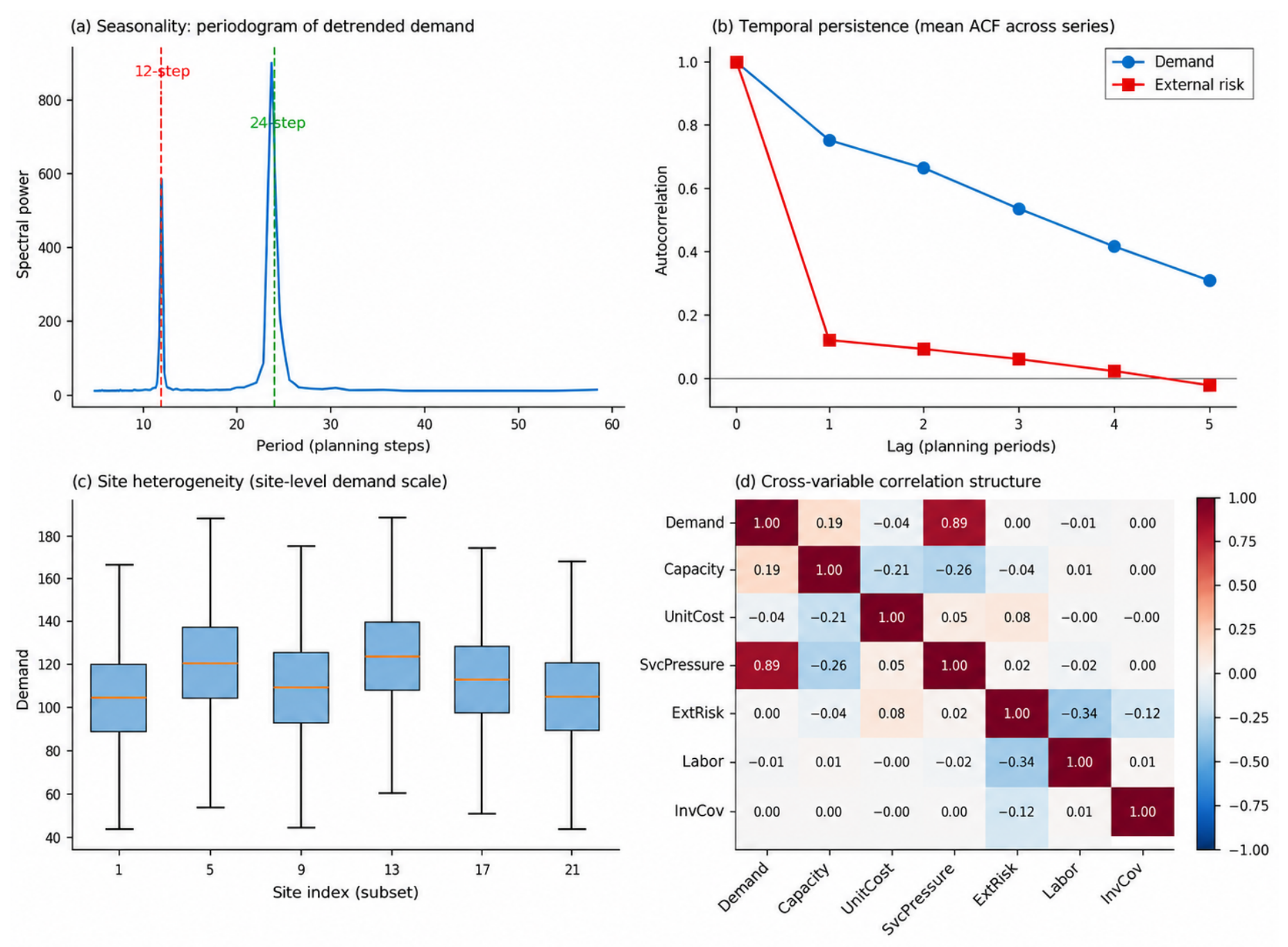
- Why this does not favor GATrESN.
Three properties of the DGP are relevant to assessing whether the synthetic environment was constructed in a way that advantages the proposed model. First, all three decision mechanisms (GATrESN, LP-Simplified, Rule-Based) receive identical input records ; none have access to , , , , or the random seeds, so none can exploit knowledge of the generating mechanism directly. Second, the nonlinear threshold terms in Equation (A6) (, ) and the intermittent, low-probability shocks in and are sources of genuine unpredictability rather than smooth, easily learned structure; they penalize any model, including GATrESN, that relies on recent history alone, and they are the reason the Monte Carlo scenario layer (Section 3.5) rather than the forecasting layer is responsible for capturing tail risk. Third, the LP-Simplified benchmark is not artificially weakened: it optimizes the same linear cost–capacity trade-off structure that dominates the trend and site/product-scale terms of Equations (A1)–(A3) (which explain the majority of variance, per the decomposition above), so a substantial share of the generated variation is, by construction, within reach of a linear planning approach. The performance gap reported in Section 4 therefore reflects GATrESN’s ability to exploit the temporal, cross-site, and disruption-coupled structure that a linear or Rule-Based policy cannot represent, rather than an artifact of a DGP tuned to make simple baselines fail.
Appendix B. Objective-Function and Optimizer Ablation
The dominance rates and paired effect sizes reported in Table 6 and Section 4 are large and consistent across service level, residual risk, and strategic score alike ( up to 8.56, dominance rates up to 100.00%). Because GATrESN’s decision is the direct output of a genetic algorithm that maximizes robustStrategicUtility (Equation (21)), while the same function is subsequently used to score all three models in Table 5, a specific and legitimate methodological concern remains regardless of effect-size magnitude: the objective function and the optimization mechanism may structurally favor the proposed solution rather than reflect a genuine predictive–prescriptive advantage. We treat this as a design property to be isolated and tested empirically rather than argued away.
- The confound has two components.
All three decision mechanisms are evaluated by the same deterministic function evaluateStrategicDecision (Equation (20)), so the scoring itself is not biased. What differs is how each mechanism selects its decision : GATrESN’s GA directly maximizes a Monte-Carlo-robust version of the same scenario-utility function it is later scored on; LP-Simplified minimizes an unrelated linear cost objective subject to service- and risk-level constraints (Equation (25)); and Rule-Based applies fixed threshold rules with no optimization at all. The comparison therefore conflates two distinct sources of advantage: which objective is pursued, and which search mechanism pursues it.
- GA-Linear ablation: isolating the mechanism from the objective.
To separate these two sources, we constructed a third decision mechanism, GA-Linear, that uses the identical genetic-algorithm search procedure as GATrESN (same simpleGA routine, population size, generation count, mutation rate, and decision-space bounds ) but optimizes LP-Simplified’s linear cost objective under the same service- and risk-level constraints, instead of the robust strategic utility. If GA-Linear scores close to LP-Simplified, the advantage of GATrESN traces to what is optimized, not how it is optimized; if GA-Linear instead scores close to GATrESN, the GA mechanism itself would be implicated. Table A2 and Figure A2a report the result: GA-Linear (mean strategic score 0.763) remains close to LP-Simplified (0.760), with a small mechanism effect in GA-Linear’s favor (paired mean advantage 0.0030, bootstrap 95% CI , entirely positive; dominance rate 91.6%; ). GATrESN (0.819) remains ahead of GA-Linear by a much larger margin (paired mean advantage 0.0566, bootstrap 95% CI ; dominance rate 100.00%; ), and the combined GATrESN-vs-LP-Simplified effect (mean advantage 0.0596, dominance 100.00%, ) is consistent with the paired statistical validation in Table 6. Replacing LP-Simplified’s search mechanism with the same GA used by GATrESN therefore contributes a small effect on its own, while the objective substitution, from a linear cost criterion to the robust strategic utility, accounts for nearly the entire gap: the objective effect () is roughly an order of magnitude larger than the mechanism effect (). This is a materially cleaner decomposition than a naive reading of the combined effect alone would suggest; we report the exact magnitudes here rather than a qualitative statement, because the ablation is intended to quantify, not merely confirm, the objective-vs-mechanism decomposition.
Table A2.
GA-Linear ablation: decomposing the GATrESN advantage into an objective effect and a mechanism effect. GA-Linear uses the same genetic-algorithm search as GATrESN but optimizes LP-Simplified’s linear objective under the same constraints.
- Weight-sensitivity analysis: is the ranking an artifact of the chosen weights?
A second, related concern is that the ranking GATrESN > LP-Simplified/Rule-Based could be an artifact of the specific weights chosen for the scenario-utility function (Equation (20)), rather than a robust property of the three policies. We re-scored the fixed decisions already selected by GATrESN, LP-Simplified, and Rule-Based (i.e., without re-optimizing) under 500 alternative weight vectors sampled from a Dirichlet distribution centered on the paper’s weights, spanning . GATrESN ranked first in 87.8% of the 500 draws and in 97.4% of a second, tighter sample restricted to within approximately of the paper’s weights. Figure A2b shows the mechanism of the exception: GATrESN’s margin over the best benchmark declines monotonically as the cost weight increases, and LP-Simplified overtakes GATrESN only once exceeds approximately , well above the weight actually used in this paper (). This is consistent with, rather than contradicting, the cost–risk trade-off already reported in Section 4: GATrESN’s advantage is a property of a decision-maker that weighs service and risk substantially alongside cost, and it attenuates, predictably rather than erratically, as the utility function is pushed toward a purely cost-minimizing objective. Because the paper’s own weight () sits comfortably below this crossover, the ranking reported throughout this paper should be read as robust for any decision-maker who does not weight cost roughly twice as heavily as the paper’s own configuration.
Figure A2.
Isolating the source of the GATrESN advantage. (a) Mean strategic score for Rule-Based, LP-Simplified, GA-Linear, and GATrESN; replacing LP-Simplified’s search mechanism with the GA used by GATrESN (GA-Linear) produces a small mechanism effect (), while replacing its objective with the robust strategic utility (GATrESN) produces a much larger objective effect (), roughly an order of magnitude greater. (b) GATrESN’s margin over the best-scoring benchmark, evaluated under 500 Dirichlet-sampled scenario-utility weight vectors, as a function of the cost weight ; the vertical line marks the weight used throughout this paper (), well below the crossover at .
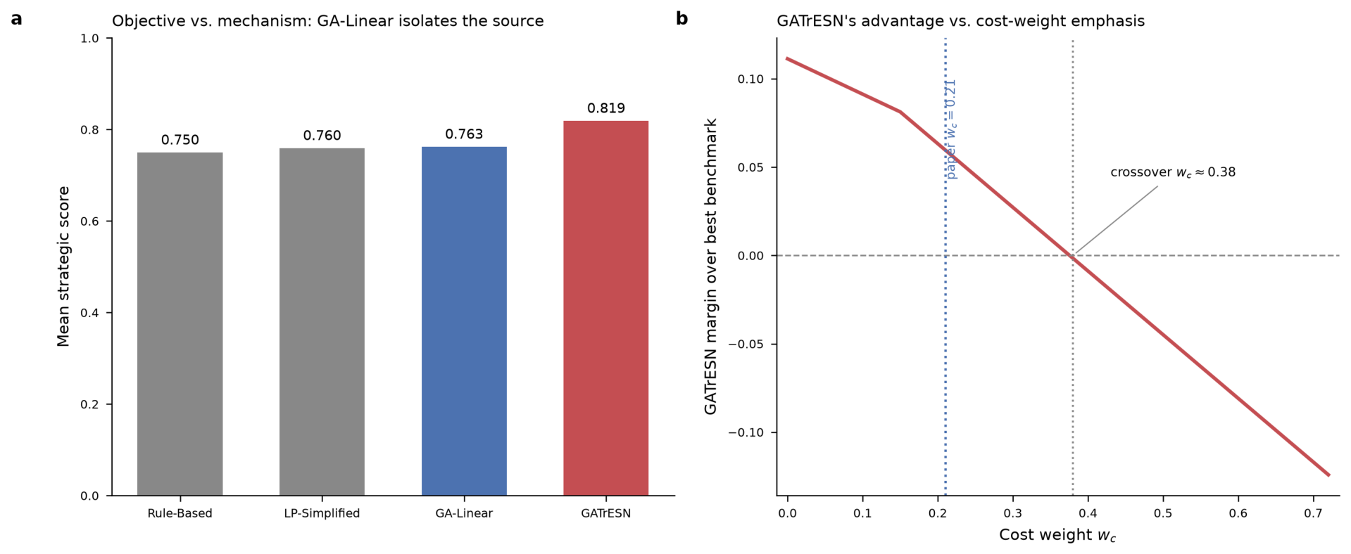
- Interpretation.
Together, the two analyses indicate that the reported superiority of GATrESN is not an artifact of granting its optimizer privileged access to the evaluation metric: an equally privileged optimizer pursuing LP-Simplified’s objective does not reproduce the advantage, and the ranking is stable under substantial perturbation of the utility weights except in the region where cost is deliberately made to dominate service and risk (Section 4.11 presents this exceptional region as a concrete named managerial profile rather than only as a continuous sweep). The remaining, narrower claim, that GATrESN’s objective function is itself richer than a linear cost criterion, and that GATrESN is the only mechanism evaluated that can pursue that richer objective directly because its threshold and percentile-based terms are not linear-programming-expressible, is a genuine design choice rather than a confound and is stated explicitly here rather than left implicit.
Appendix C. Series Independence and Boundary Resets
The case-study panel is organized as a family of site–product series , and nothing in the data-generating process defines consecutive series in the group-major row ordering (e.g., followed by ) as temporally adjacent trajectories: they are distinct operational units that happen to be adjacent only because of how rows are concatenated for matrix construction. An earlier version of the predictive core processed all rows in a single pass without resetting state at series boundaries, which would implicitly treat unrelated series as one continuous sequence. The reported pipeline avoids this: as described in Section 3.6, a series-boundary group identifier is tracked for every row, and both the ESN reservoir state (Equation (8)) and the lagged attention context window (Equation (9)) are reset at every site–product series boundary, so no state or attention weight ever propagates from one series into an unrelated one. All results reported in this paper, including the forecasting metrics (Table 3), the benchmark comparison (Table 5), the statistical validation (Table 6), and the predictive ablation (Table 4), are computed under this boundary-reset implementation.
References
- Tao, F.; Zhang, H.; Liu, A.; Nee, A.Y.C. Digital twin in industry: State-of-the-art. IEEE Trans. Ind. Inform. 2019, 15, 2405–2415. [Google Scholar] [CrossRef] [Scilit]
- Fuller, A.; Fan, Z.; Day, C.; Barlow, C. Digital Twin: Enabling Technologies, Challenges and Open Research. IEEE Access 2020, 8, 108952–108971. [Google Scholar] [CrossRef] [Scilit]
- Kritzinger, W.; Karner, M.; Traar, G.; Henjes, J.; Sihn, W. Digital Twin in manufacturing: A categorical literature review and classification. IFAC-PapersOnLine 2018, 51, 1016–1022. [Google Scholar] [CrossRef] [Scilit]
- Jaeger, H.; Haas, H. Harnessing Nonlinearity: Predicting Chaotic Systems and Saving Energy in Wireless Communication. Science 2004, 304, 78–80. [Google Scholar] [CrossRef] [Scilit] [PubMed]
- Lukoševičius, M.; Jaeger, H. Reservoir computing approaches to recurrent neural network training. Comput. Sci. Rev. 2009, 3, 127–149. [Google Scholar] [CrossRef] [Scilit]
- Niu, Z.; Zhong, G.; Yu, H. A review on the attention mechanism of deep learning. Neurocomputing 2021, 452, 48–62. [Google Scholar] [CrossRef] [Scilit]
- Vaswani, A.; Shazeer, N.; Parmar, N.; Uszkoreit, J.; Jones, L.; Gomez, A.N.; Kaiser, L.; Polosukhin, I. Attention Is All You Need. In Proceedings of the Advances in Neural Information Processing Systems 30 (NIPS 2017), Long Beach, CA, USA; Neural Information Processing Systems Foundation, Inc. (NeurIPS): La Jolla, CA, USA, 2017; pp. 5998–6008. [Google Scholar]
- Deb, K.; Pratap, A.; Agarwal, S.; Meyarivan, T. A fast and elitist multiobjective genetic algorithm: NSGA-II. IEEE Trans. Evol. Comput. 2002, 6, 182–197. [Google Scholar] [CrossRef] [Scilit]
- Tao, F.; Cheng, J.; Qi, Q.; Zhang, M.; Zhang, H.; Sui, F. Digital twin-driven product design, manufacturing and service with big data. Int. J. Adv. Manuf. Technol. 2018, 94, 3563–3576. [Google Scholar] [CrossRef] [Scilit]
- Moshood, T.; Nawanir, G.; Sorooshian, S.; Okfalisa, O. Digital Twins Driven Supply Chain Visibility within Logistics: A New Paradigm for Future Logistics. Appl. Syst. Innov. 2021, 4, 29. [Google Scholar] [CrossRef] [Scilit]
- Soori, M.; Arezoo, B.; Dastres, R. Digital twin for smart manufacturing, A review. Sustain. Manuf. Serv. Econ. 2023, 2, 100017. [Google Scholar] [CrossRef] [Scilit]
- Kusiak, A. Smart manufacturing. Int. J. Prod. Res. 2018, 56, 508–517. [Google Scholar] [CrossRef] [Scilit]
- Ding, K.; Chan, F.T.S.; Zhang, X.; Zhou, G.; Zhang, F. Defining a Digital Twin-based Cyber-Physical Production System for autonomous manufacturing in smart shop floors. Int. J. Prod. Res. 2019, 57, 6315–6334. [Google Scholar] [CrossRef] [Scilit]
- Zhou, G.; Zhang, C.; Li, Z.; Ding, K.; Wang, C. Knowledge-driven digital twin manufacturing cell towards intelligent manufacturing. Int. J. Prod. Res. 2020, 58, 1034–1051. [Google Scholar] [CrossRef] [Scilit]
- Qi, Q.; Tao, F. Digital Twin and Big Data Towards Smart Manufacturing and Industry 4.0: 360 Degree Comparison. IEEE Access 2018, 6, 3585–3593. [Google Scholar] [CrossRef] [Scilit]
- Fatorachian, H.; Kazemi, H. Impact of Industry 4.0 on supply chain performance. Prod. Plan. Control 2021, 32, 63–81. [Google Scholar] [CrossRef] [Scilit]
- Rasheed, A.; San, O.; Kvamsdal, T. Digital Twin: Values, Challenges and Enablers From a Modeling Perspective. IEEE Access 2020, 8, 21980–22012. [Google Scholar] [CrossRef] [Scilit]
- Fanoro, M.; Božanić, M.; Sinha, S. A Review of 4IR/5IR Enabling Technologies and Their Linkage to Manufacturing Supply Chain. Technologies 2021, 9, 77. [Google Scholar] [CrossRef] [Scilit]
- Stavropoulos, P. Digitization of Manufacturing Processes: From Sensing to Twining. Technologies 2022, 10, 98. [Google Scholar] [CrossRef] [Scilit]
- Martinez-Ruedas, C.; Flores-Arias, J.M.; Moreno-Garcia, I.M.; Linan-Reyes, M.; Bellido-Outeiriño, F.J. A Cyber–Physical System Based on Digital Twin and 3D SCADA for Real-Time Monitoring of Olive Oil Mills. Technologies 2024, 12, 60. [Google Scholar] [CrossRef] [Scilit]
- Ivanov, D.; Dolgui, A. Digital supply chain twin for managing the disruption risks and resilience in the era of Industry 4.0. Prod. Plan. Control 2021, 32, 775–788. [Google Scholar] [CrossRef] [Scilit]
- Ivanov, D.; Dolgui, A.; Sokolov, B. The impact of digital technology and Industry 4.0 on the ripple effect and supply chain risk analytics. Int. J. Prod. Res. 2019, 57, 829–846. [Google Scholar] [CrossRef] [Scilit]
- Burgos, D.; Ivanov, D. Food retail supply chain resilience and the COVID-19 pandemic: A digital twin-based impact analysis and improvement directions. Transp. Res. Part E Logist. Transp. Rev. 2021, 152, 102412. [Google Scholar] [CrossRef] [Scilit] [PubMed]
- Ivanov, D. Intelligent digital twin (iDT) for supply chain stress-testing, resilience, and viability. Int. J. Prod. Econ. 2023, 263, 108938. [Google Scholar] [CrossRef] [Scilit]
- Ivanov, D.; Dolgui, A.; Sokolov, B. Cloud supply chain: Integrating Industry 4.0 and digital platforms in the Supply Chain-as-a-Service. Transp. Res. Part E Logist. Transp. Rev. 2022, 160, 102676. [Google Scholar] [CrossRef] [Scilit]
- Fang, Y.; Peng, C.; Lou, P.; Zhou, Z.; Hu, J.; Yan, J. Digital-Twin-Based Job Shop Scheduling Toward Smart Manufacturing. IEEE Trans. Ind. Inform. 2019, 15, 6425–6435. [Google Scholar] [CrossRef] [Scilit]
- Zhang, M.; Tao, F.; Nee, A.Y.C. Digital Twin Enhanced Dynamic Job-Shop Scheduling. J. Manuf. Syst. 2021, 58, 146–156. [Google Scholar] [CrossRef] [Scilit]
- Lugaresi, G.; Matta, A. Automated manufacturing system discovery and digital twin generation. J. Manuf. Syst. 2021, 59, 51–66. [Google Scholar] [CrossRef] [Scilit]
- Wang, G.; Zhang, G.; Guo, X.; Zhang, Y. Digital twin-driven service model and optimal allocation of manufacturing resources in shared manufacturing. J. Manuf. Syst. 2021, 59, 165–179. [Google Scholar] [CrossRef] [Scilit]
- Ouahabi, N.; Chebak, A.; Kamach, O.; Laayati, O.; Zegrari, M. Leveraging digital twin into dynamic production scheduling: A review. Robot. Comput.-Integr. Manuf. 2024, 89, 102778. [Google Scholar] [CrossRef] [Scilit]
- Toorajipour, R.; Sohrabpour, V.; Nazarpour, A.; Oghazi, P.; Fischl, M. Artificial intelligence in supply chain management: A systematic literature review. J. Bus. Res. 2021, 122, 502–517. [Google Scholar] [CrossRef] [Scilit]
- Huang, T.; Bergman, D.; Gopal, R. Predictive and Prescriptive Analytics for Location Selection of Add-on Retail Products. Prod. Oper. Manag. 2019, 28, 1858–1877. [Google Scholar] [CrossRef] [Scilit]
- Bertsimas, D.; Kallus, N. From Predictive to Prescriptive Analytics. Manag. Sci. 2020, 66, 1025–1044. [Google Scholar] [CrossRef] [Scilit]
- Kilimci, Z.H.; Akyuz, A.O.; Uysal, M.; Akyokus, S.; Uysal, M.O.; Atak Bulbul, B.; Ekmis, M.A. An Improved Demand Forecasting Model Using Deep Learning Approach and Proposed Decision Integration Strategy for Supply Chain. Complexity 2019, 2019, 9067367. [Google Scholar] [CrossRef] [Scilit]
- Gauthier, D.J.; Bollt, E.; Griffith, A.; Barbosa, W.A.S. Next generation reservoir computing. Nat. Commun. 2021, 12, 5564. [Google Scholar] [CrossRef] [Scilit] [PubMed]
- Maass, W.; Natschläger, T.; Markram, H. Real-time computing without stable states: A new framework for neural computation based on perturbations. Neural Comput. 2002, 14, 2531–2560. [Google Scholar] [CrossRef] [Scilit] [PubMed]
- Cucchi, M.; Abreu, S.; Ciccone, G.; Brunner, D.; Kleemann, H. Hands-on reservoir computing: A tutorial for practical implementation. Neuromorphic Comput. Eng. 2022, 2, 032002. [Google Scholar] [CrossRef] [Scilit]
- Valencia, C.; Vellasco, M.; Figueiredo, K. Echo State Networks: Novel reservoir selection and hyperparameter optimization model for time series forecasting. Neurocomputing 2023, 545, 126317. [Google Scholar] [CrossRef] [Scilit]
- Zhou, H.; Zhang, S.; Peng, J.; Zhang, S.; Li, J.; Xiong, H.; Zhang, W. Informer: Beyond Efficient Transformer for Long Sequence Time-Series Forecasting. Proc. AAAI Conf. Artif. Intell. 2021, 35, 11106–11115. [Google Scholar] [CrossRef] [Scilit]
- López Santos, M.; García-Santiago, X.; Echevarría Camarero, F.; Blázquez Gil, G.; Carrasco Ortega, P. Application of Temporal Fusion Transformer for Day-Ahead PV Power Forecasting. Energies 2022, 15, 5232. [Google Scholar] [CrossRef] [Scilit]
- Valencia-Niño, C.; Nuñez-Rodriguez, R.; Vellasco, M.; Marin, J. ESNformer: A Hybrid Reservoir–Transformer Architecture for Interpretable, Position-Aware Classification of Structured Assessment Data, with a Braille-Literacy Case Study. Technologies 2026, 14, 517. [Google Scholar] [CrossRef] [Scilit]
- Elmachtoub, A.N.; Grigas, P. Smart “Predict, then Optimize”. Manag. Sci. 2022, 68, 9–26. [Google Scholar] [CrossRef] [Scilit]
- Mandi, J.; Kotary, J.; Berden, S.; Mulamba, M.; Bucarey, V.; Guns, T.; Fioretto, F. Decision-Focused Learning: Foundations, State of the Art, Benchmark and Future Opportunities. J. Artif. Intell. Res. 2024, 80, 1623–1701. [Google Scholar] [CrossRef] [Scilit]
- Zhao, S.; You, F. Resilient supply chain design and operations with decision-dependent uncertainty using a data-driven robust optimization approach. AIChE J. 2019, 65, 1006–1021. [Google Scholar] [CrossRef] [Scilit]
- Gumte, K.M.; Devi Pantula, P.; Miriyala, S.S.; Mitra, K. Data driven robust optimization for handling uncertainty in supply chain planning models. Chem. Eng. Sci. 2021, 246, 116889. [Google Scholar] [CrossRef] [Scilit]
- Fattahi, M.; Govindan, K.; Maihami, R. Stochastic optimization of disruption-driven supply chain network design with a new resilience metric. Int. J. Prod. Econ. 2020, 230, 107755. [Google Scholar] [CrossRef] [Scilit]
- Lejarza, F.; Kelley, M.T.; Baldea, M. Feedback-Based Deterministic Optimization Is a Robust Approach for Supply Chain Management under Demand Uncertainty. Ind. Eng. Chem. Res. 2022, 61, 12153–12168. [Google Scholar] [CrossRef] [Scilit]
- Chen, S.; Chen, Y. Designing a resilient supply chain network: A multi-objective data-driven distributionally robust optimization method. Comput. Oper. Res. 2025, 173, 106868. [Google Scholar] [CrossRef] [Scilit]
- Rockafellar, R.; Uryasev, S. Conditional value-at-risk for general loss distributions. J. Bank. Financ. 2002, 26, 1443–1471. [Google Scholar] [CrossRef] [Scilit]
- Chen, D.; Sain, S.L.; Guo, K. Data mining for the online retail industry: A case study of RFM model-based customer segmentation using data mining. J. Database Mark. Cust. Strategy Manag. 2012, 19, 197–208. [Google Scholar] [CrossRef] [Scilit]
- Lundberg, S.M.; Erion, G.; Chen, H.; DeGrave, A.; Prutkin, J.M.; Nair, B.; Katz, R.; Himmelfarb, J.; Bansal, N.; Lee, S.I. From local explanations to global understanding with explainable AI for trees. Nat. Mach. Intell. 2020, 2, 56–67. [Google Scholar] [CrossRef] [Scilit] [PubMed]
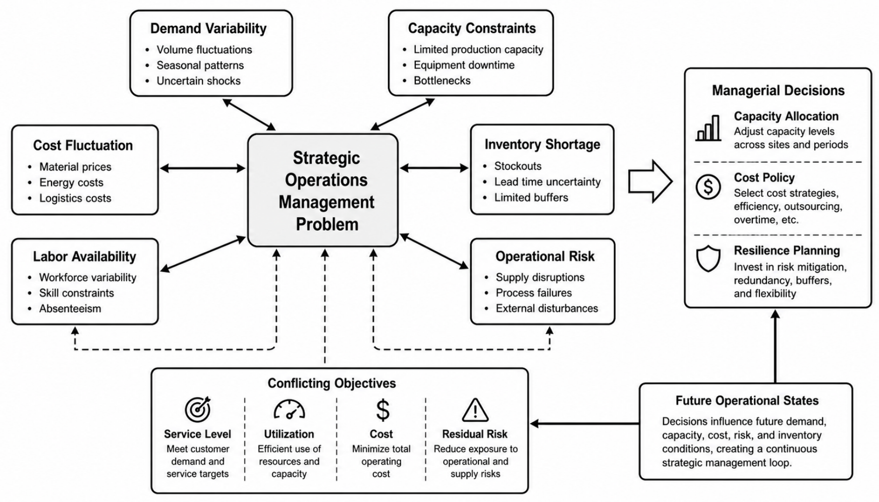
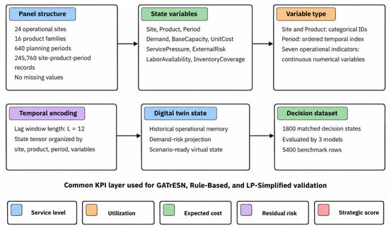
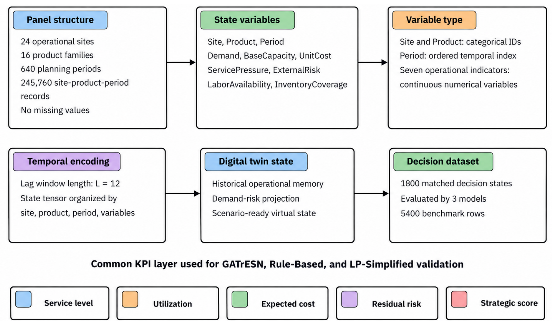
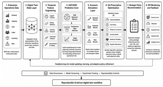
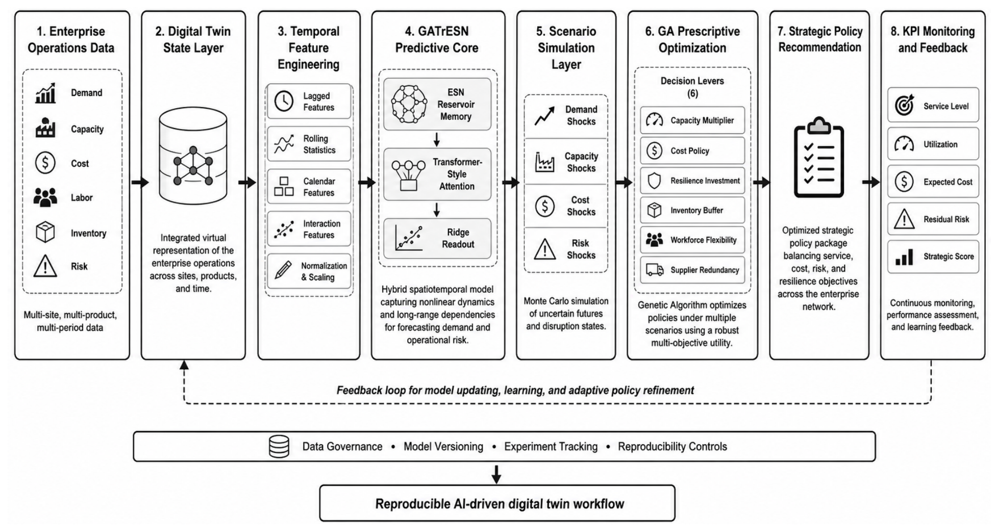
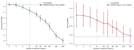
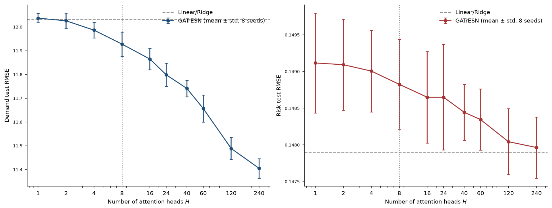
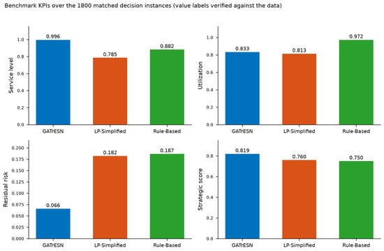
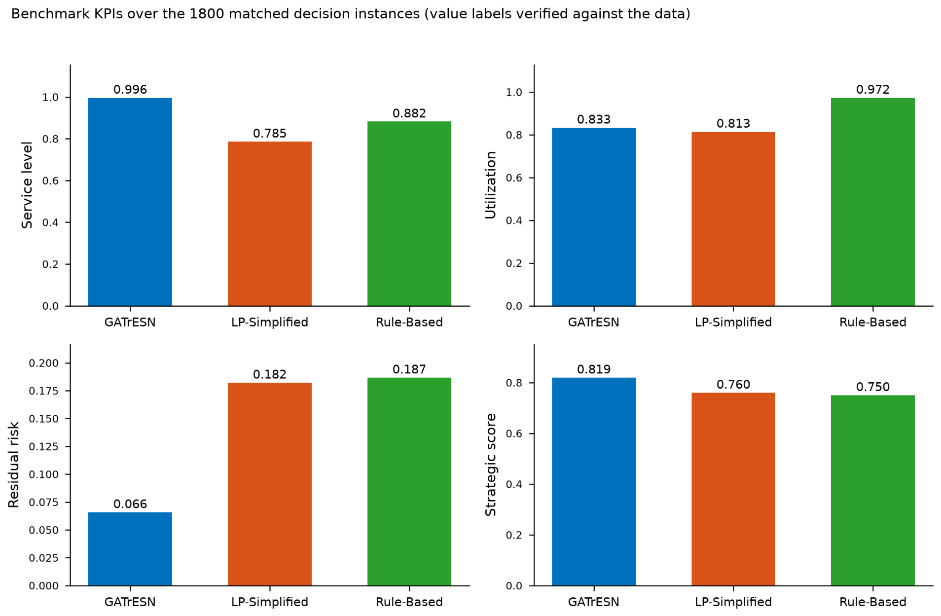
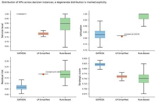
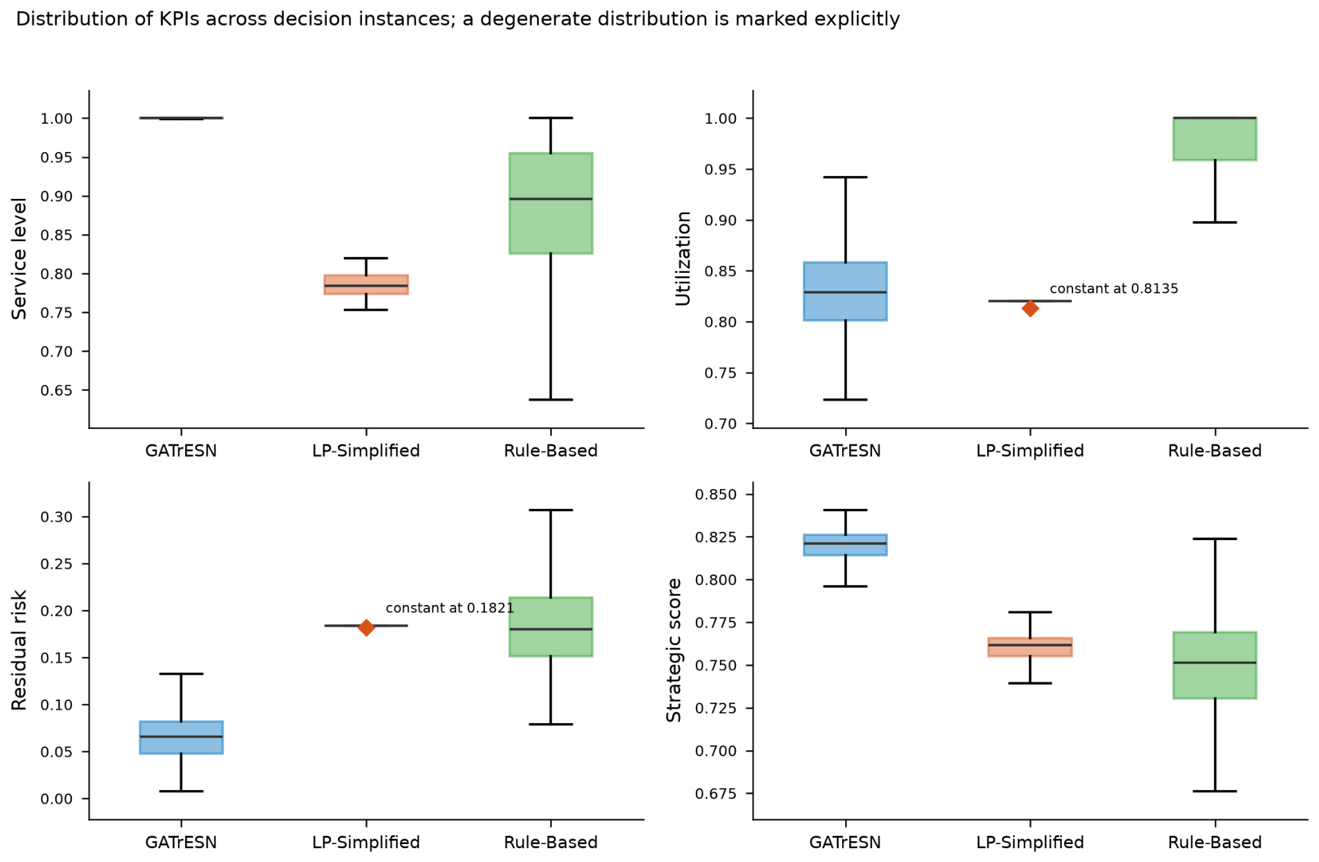
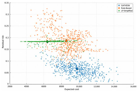
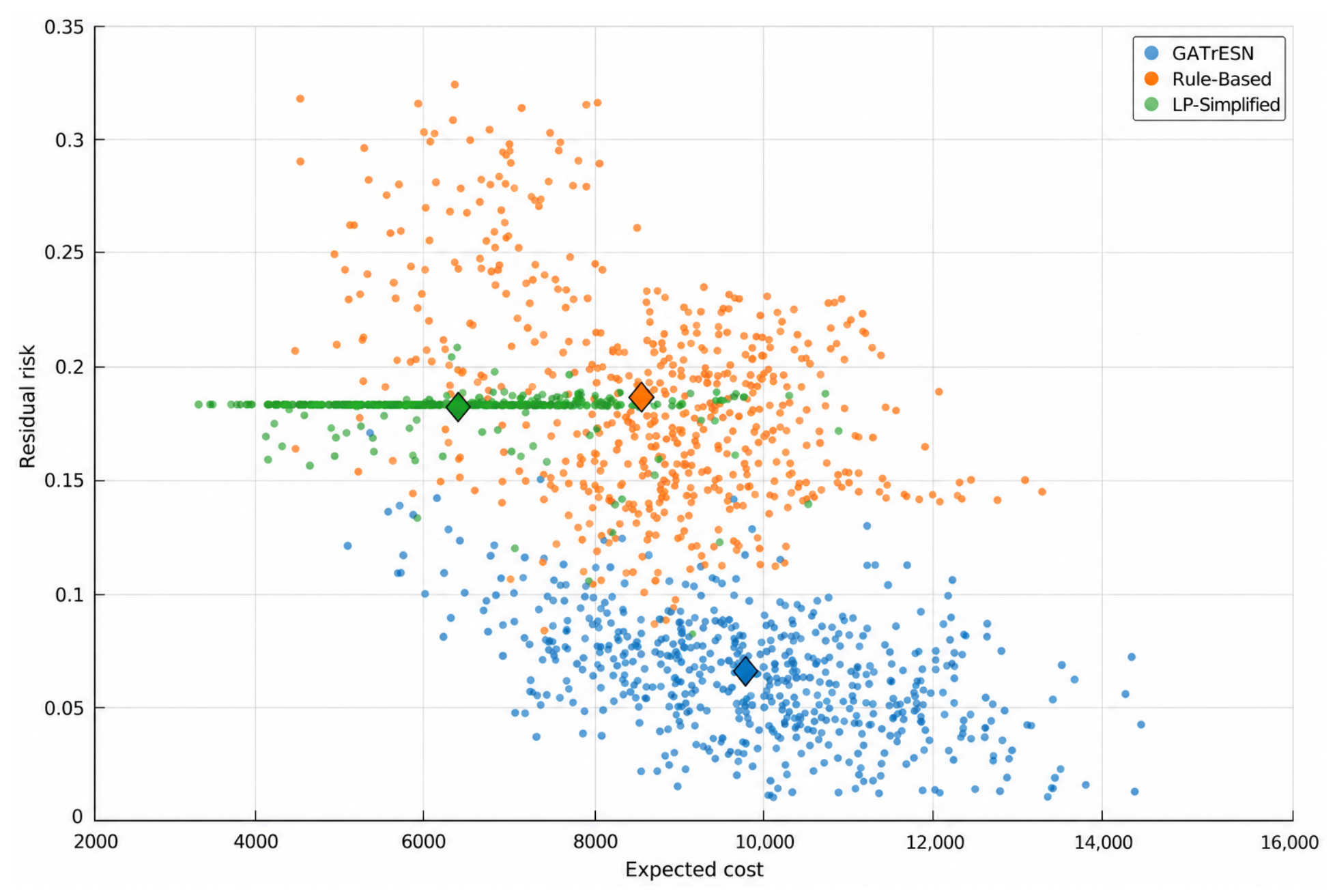
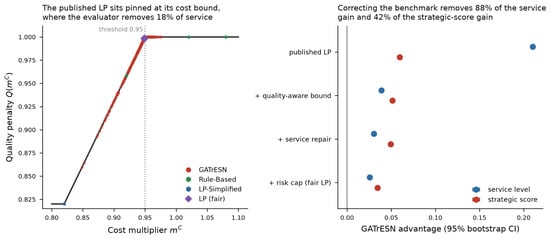
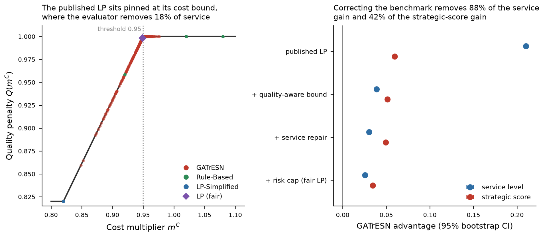
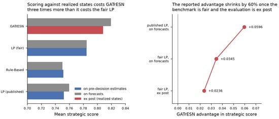
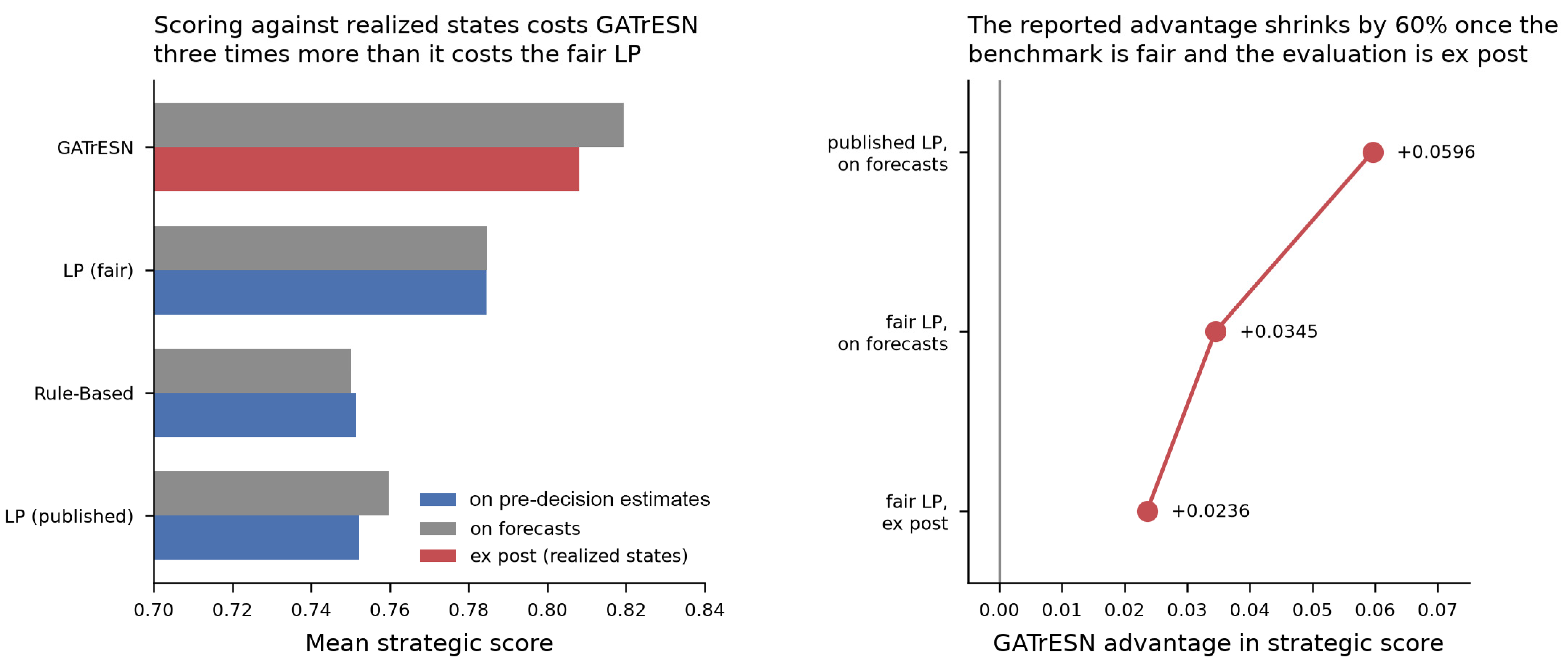
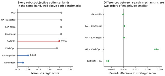
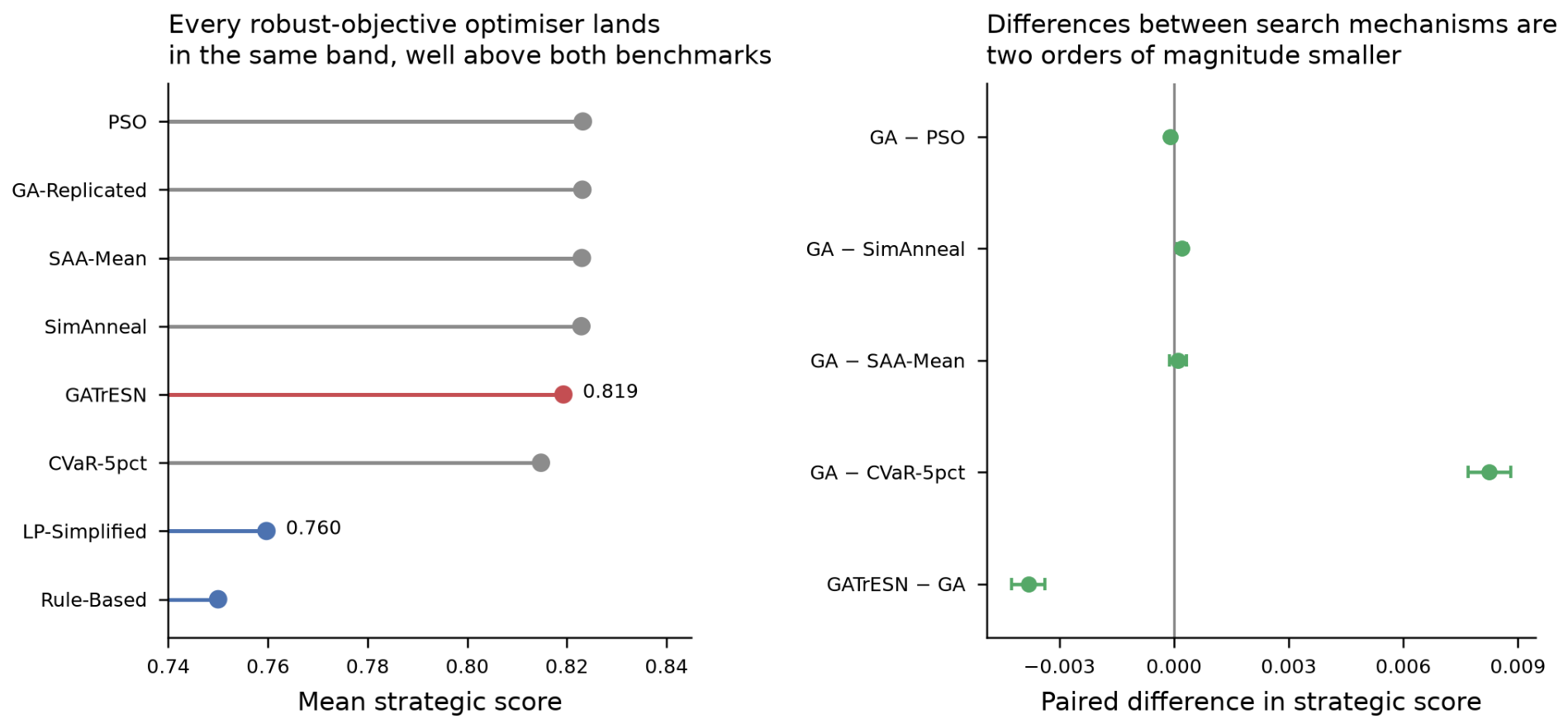
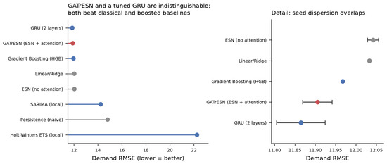
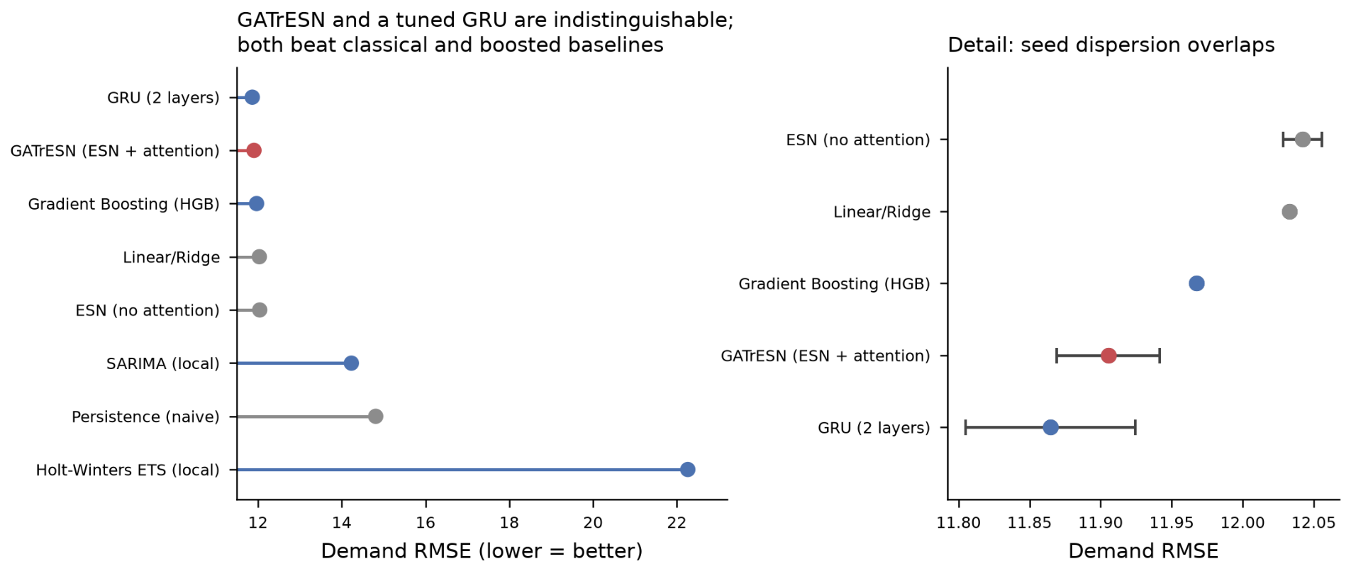
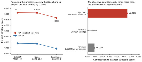
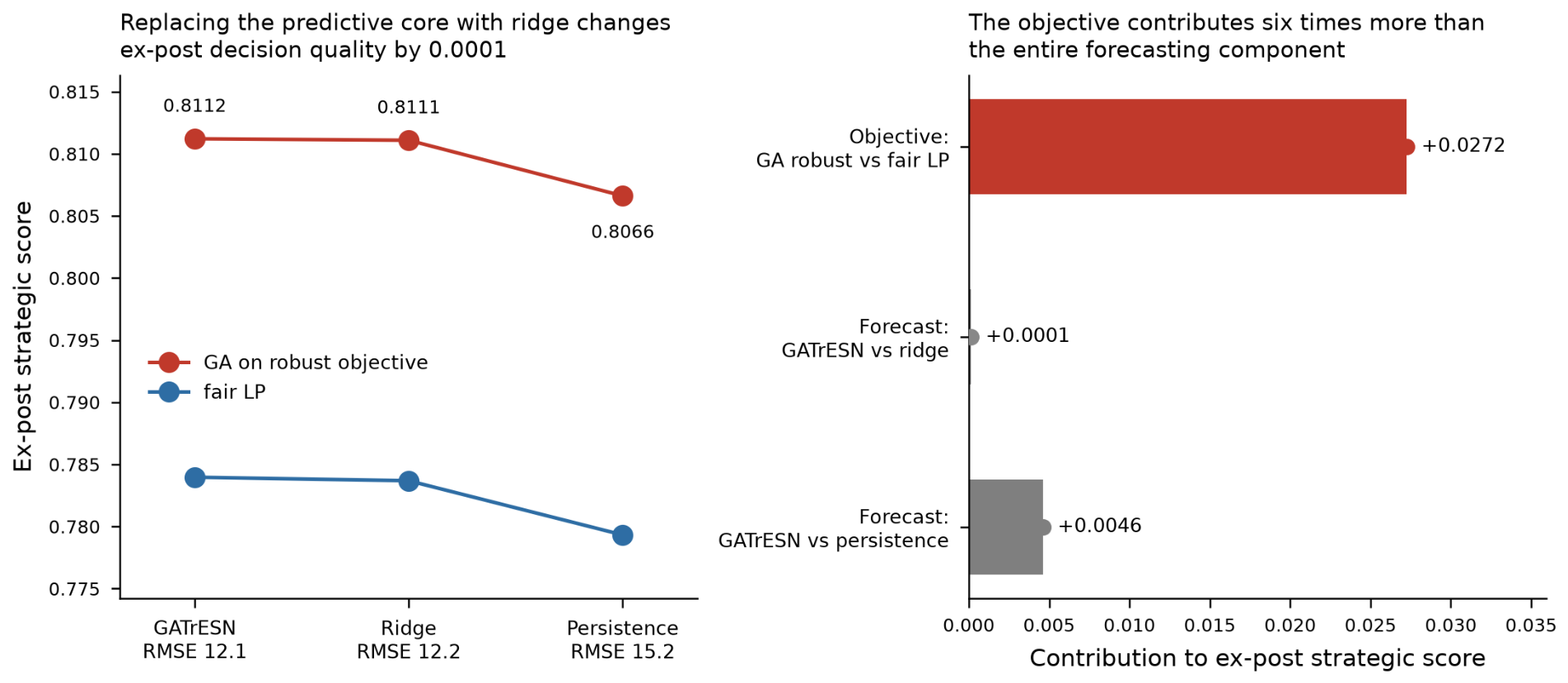
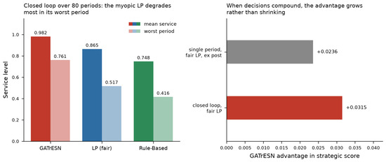
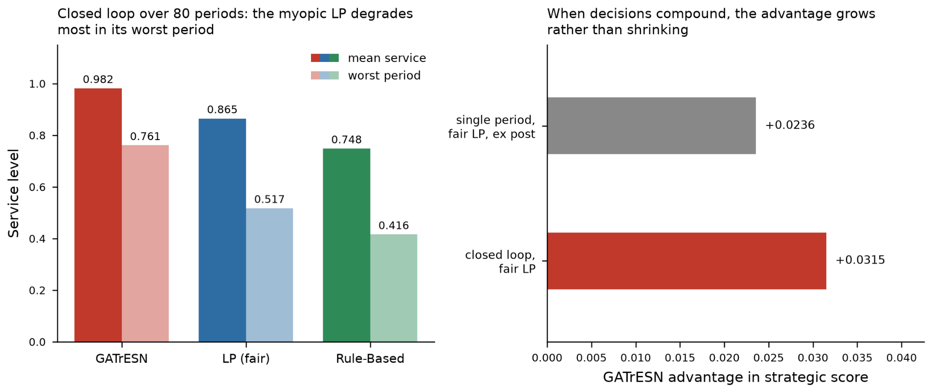
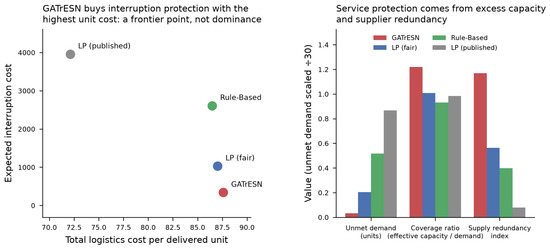
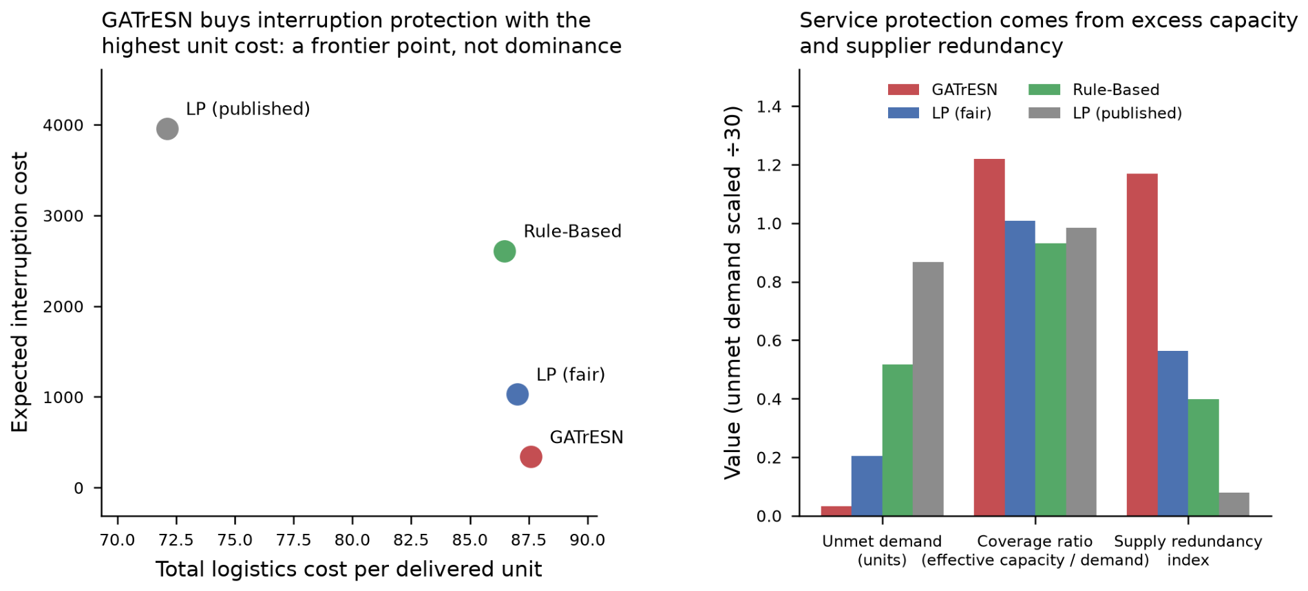
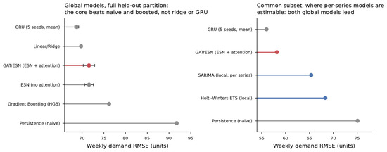
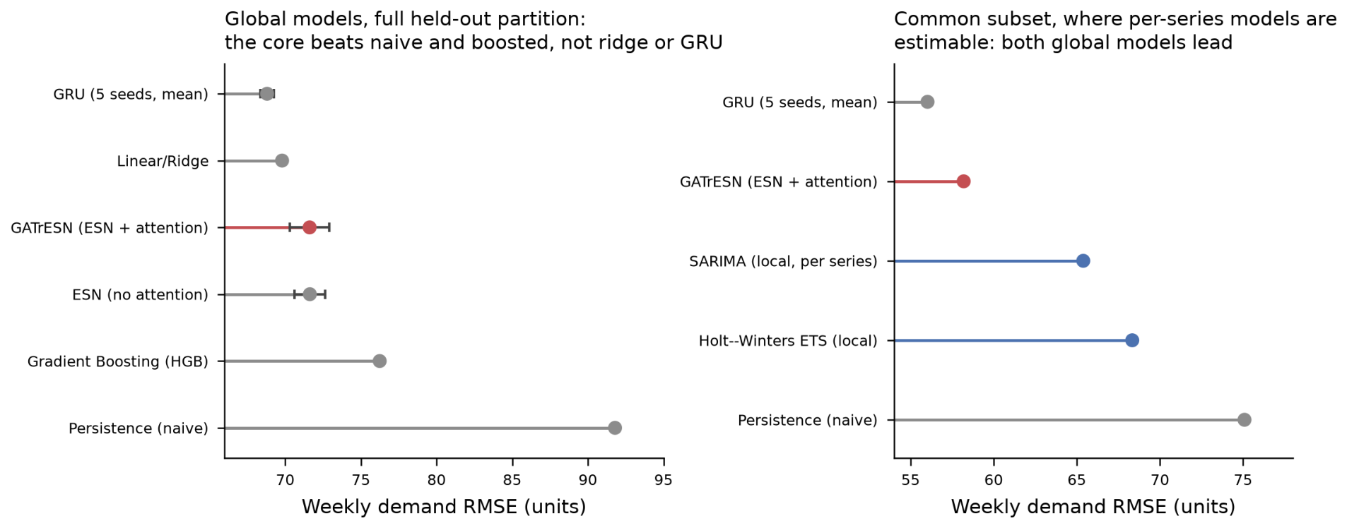
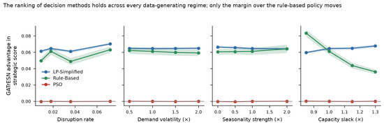
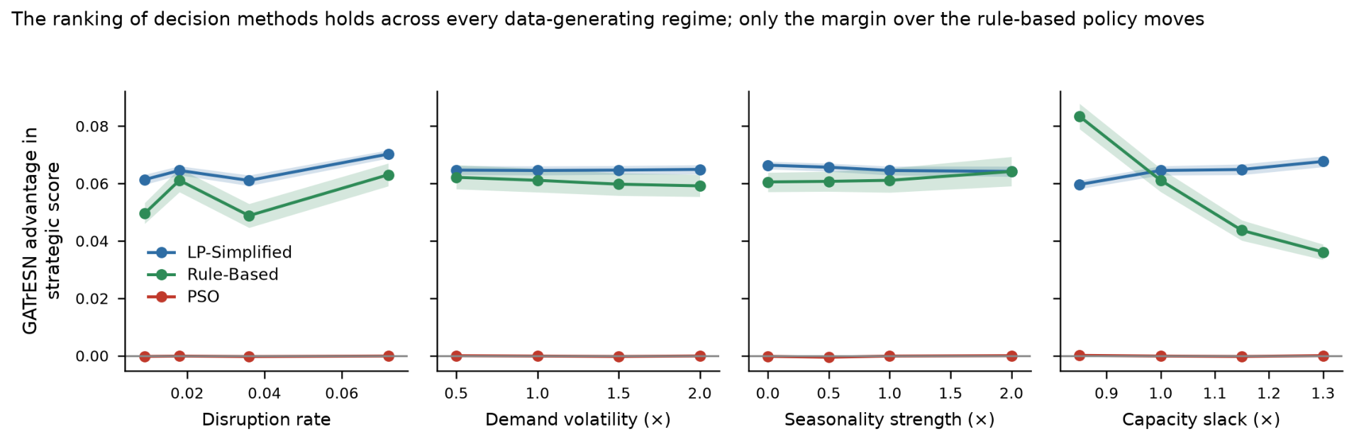
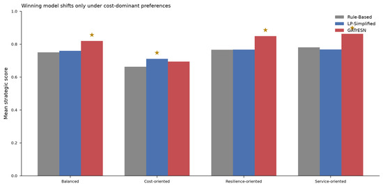
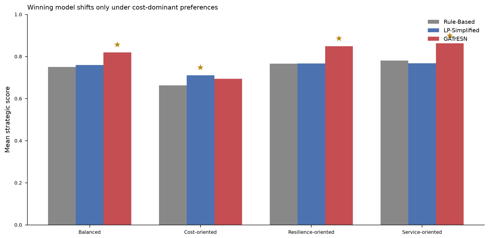
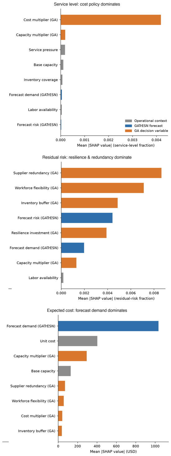
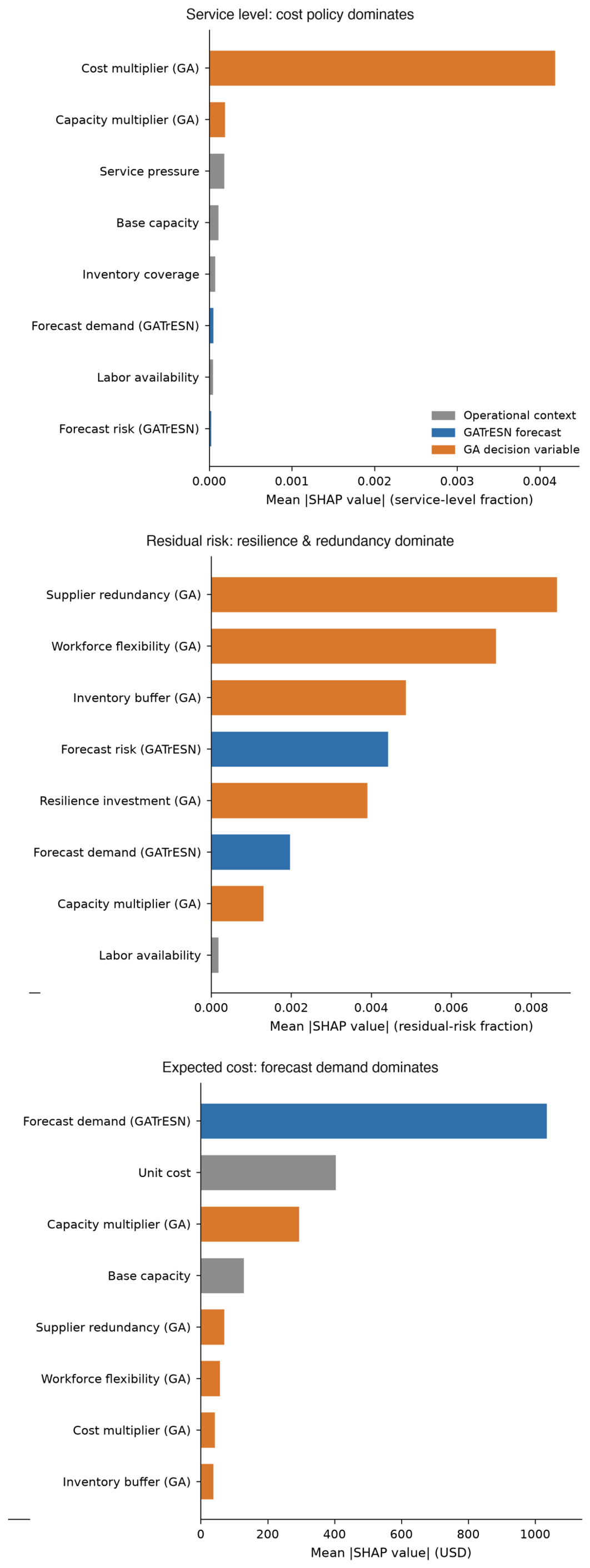
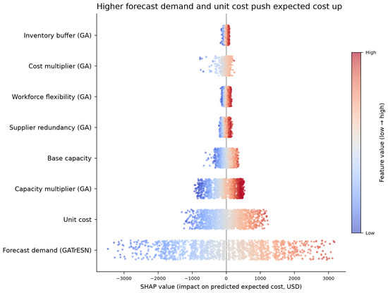
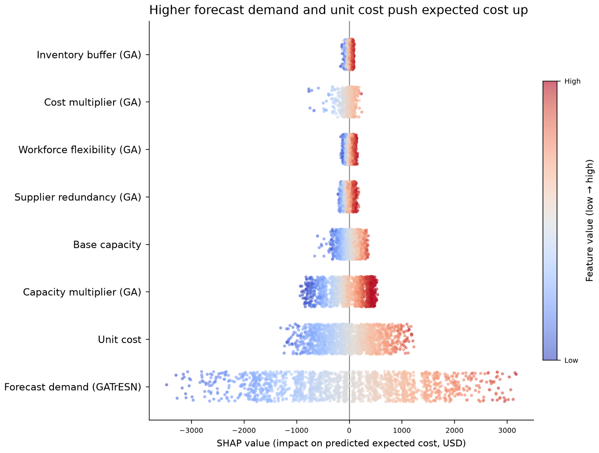
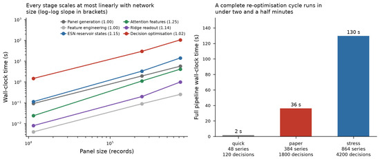
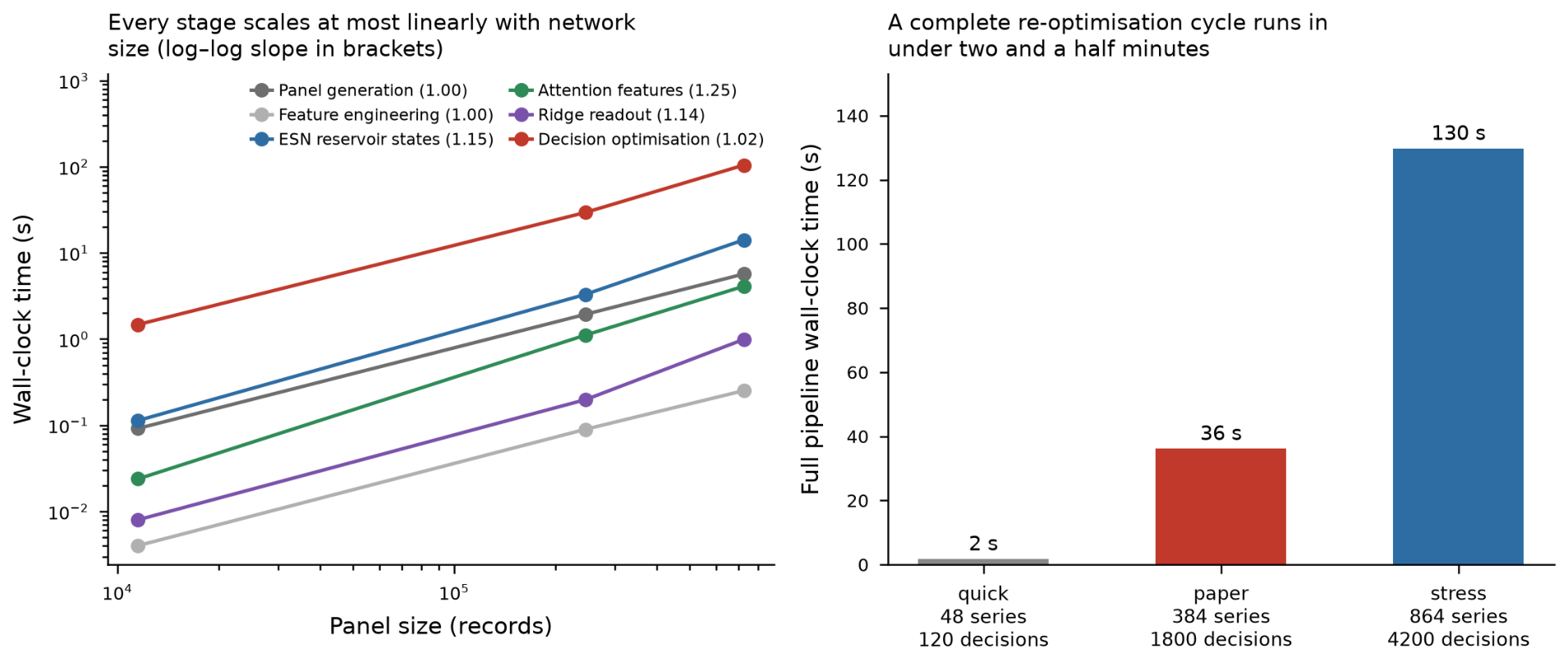

Disclaimer/Publisher’s Note: The statements, opinions and data contained in all publications are solely those of the individual author(s) and contributor(s) and not of MDPI and/or the editor(s). MDPI and/or the editor(s) disclaim responsibility for any injury to people or property resulting from any ideas, methods, instructions or products referred to in the content. |
© 2026 by the authors. Licensee MDPI, Basel, Switzerland. This article is an open access article distributed under the terms and conditions of the Creative Commons Attribution (CC BY) license.