PG-MTCDGNet: A Physics-Grounded Multi-Scale Time-Lagged Dynamic Graph Network for Structured Evidence Reporting in Planetary-Gearbox Fault Diagnosis

Abstract

Multichannel vibration from a planetary gearbox exhibits operating-condition-dependent interactions across both time scale and lag. Static undirected graphs cannot represent ordered temporal dependence, while repeated graph aggregation can attenuate localized impacts. This paper presents PG-MTCDGNet, a physics-grounded multi-scale time-lagged dynamic graph network for structured evidence reporting in planetary-gearbox fault diagnosis. Phase-synchronous X/Y vibration, transient residuals, Hilbert envelopes, cross-channel coupling, and encoder micro-speed are represented as eight physical nodes. Sparse directed graphs are induced using the angular lags of one, four, and 16 samples from lagged predictive associations and are regularized by label-independent mesh and modulation priors. A time-lagged graph branch is fused with an unsmoothed local-evidence branch, and the complete model is trained with a fold-internal noise-consistency curriculum spanning −6 to 10 dB. The WT dataset comprises 80 continuous raw files and 5120 windows from five health states, two installations, and eight speeds. Under raw-file-isolated, class-installation-speed-balanced five-fold validation, PG-MTCDGNet achieved 99.61% ± 0.33% accuracy, 99.63% ± 0.31% macro-F1, and 0.99999 macro-AUC. Accuracy at 0 dB feature noise was 96.78%. A depth-reduced variant, PG-MTCDGNet-Lite, separates comparable signal descriptors from heterogeneous physical tokens and uses a regularized linear readout. In exploratory installation and speed holdouts, its four-condition file-level accuracy was 88.125%, versus 86.250% for the matched MLP; likewise, macro-F1 was 88.044% versus 84.171%. Removing graph propagation tied its overall accuracy, so this improvement does not establish a unique graph contribution. The 80 recordings were reused during model development, and the results require confirmation on new independent recordings.

1. Introduction

Planetary gearboxes combine high-power density with compact load sharing, and are widely used in wind-energy, aerospace, and heavy-duty drivetrains. Their measured vibration, however, is shaped by planet revolution, gear rotation, multiple simultaneous mesh contacts, and a transfer path that changes with the carrier position [1]. The WT benchmark makes these effects explicit by covering five health states, two sensor installations, and eight input speeds. Reviews of planetary-gearbox diagnoses and rotating machinery under time-varying speeds show that speed fluctuation broadens fault-related spectral components and weakens the transferability of fixed-frequency features [2].

While deep models reduce reliance on handcrafted descriptors, they can also exploit speed, installation, and sensor orientation as shortcuts [3]. Recent reviews identify graph neural networks (GNNs) as a useful means of representing relationships among sensors, frequency bands, or local signal segments, while also emphasizing that graph construction and cross-condition generalization remain unresolved [4]. Early multichannel graph convolution used parallel undirected neighborhood graphs, and spiking graph attention introduced spatiotemporal encoding for planetary-gearbox diagnosis [5,6]. These studies established the value of relational modeling, but their graphs were usually based on synchronous similarity or prescribed adjacency and therefore did not represent which channel preceded another.

Multi-scale graph convolution with contrastive pooling can aggregate gearbox information across frequency resolutions, and time-frequency similarity graphs can organize local windows into graph-level samples [7,8]. Because these approaches generally rely on symmetric distances, a directed lagged dependency is reduced to an undirected association [9]. Noise-robust multiview GNNs and richly connected spatiotemporal graphs improve complementarity and long-range information flow across sensors [10], yet they do not explicitly separate the direction of transmission at different time scales.

The 2025 ESC-DGCN model combines elastic spatial convolution, an autoregressive receptive field, and deep graph cascading for non-stationary speed conditions [11]. Work on degree-bias mitigation further shows that incorrect connections and unbalanced node degree can amplify aggregation errors under strong noise [12]. More recent mechanism-oriented models infer adaptive dependency structures or use frequency-aware graph contrastive learning [13,14]. These developments move the field from correlation graphs toward mechanism-informed representations, but file-isolated validation across both installation and speed variations remains uncommon.

A spatial–temporal decoupled graph has shown that temporal samples can themselves serve as dynamic nodes, while a spiking graph convolutional residual network has demonstrated robustness for planetary gearboxes at negative signal-to-noise ratios (SNRs) [15,16]. Heterogeneous meta-path graphs and entropy-driven multilevel fusion also integrate operating-condition and multisensor information [17,18]. Directly connecting speed or installation nodes to the diagnostic target, however, risks encoding an operating-condition shortcut. The present study therefore admits only label-independent physical relations into the graph prior.

Model outputs have been examined through adaptive fusion GCNs for heating, ventilation, and air-conditioning systems and through graph-based label propagation with virtual adversarial training for gearboxes [19,20]. Attention maps alone do not verify a physical mechanism: any proposed interpretation should be tested against counterfactual deletion, operating-condition variation, and independent physical evidence [21]. Generative one-class and semi-supervised physics-informed models address limited fault samples [22], but generated signals may introduce patterns inconsistent with the actual mesh mechanism. We instead use analytically controlled Gaussian perturbations and do not synthesize fault labels.

Encoder signals provide a physical phase reference for toothwise monitoring under variable speed, and synchro-reassigning transforms improve instantaneous-frequency estimation and reconstruction [23,24]. Proportion-extracting chirplet analysis captures non-stationary rotational components, while hypergraph models show that higher-order relations can supplement pairwise interactions [25,26]. To keep the reported dependency structure directly inspectable, this work uses pairwise directed edges from angular lags of one, four, and 16 samples, spanning short, impulsive events and slower modulation.

Multi-scale entropy and discriminative sparse autoencoders remain strong descriptors for complex vibration signals [27,28]. Modified stacked autoencoders and attention-guided denoising networks represent complementary compression and noise-rejection strategies [29,30]. We therefore include a random forest, an SAE-MLP, and a deep MLP as classical and deep baselines, and distinguish default robustness experiments from a matched-curriculum control in which all deep models receive exactly the same noisy training examples.

Signal-Transformer and health-adaptive time-scale convolution illustrate two routes toward operating-condition-invariant representations [31,32]. Local bispectrum networks and wavelet-packet multi-scale CNNs further show that non-Gaussian impacts and cross-scale energy should be retained rather than collapsed into a single spectrum [33,34]. Accordingly, the proposed node set preserves angle-domain waveforms, high-pass transients, envelopes, cross-channel coupling, and encoder-derived micro-speed information.

Convformer-NSE and efficient convolutional Transformers improve noise adaptation and long-range modeling [35,36]. Cross-domain and multisensor Transformers align conditions and fuse complementary channels through attention [37,38]. Their latent attention, however, is not necessarily a transmission direction. Multisensor and multi-scale fusion networks also confirm that sensor relevance changes with operating conditions [39,40]. We make this dependence explicit through lag-specific edges, branch-level posteriors, and node-level counterfactual deletion.

Multisensor CNNs improve cross-channel discrimination, whereas open-set studies caution that unseen faults can invalidate a closed-set boundary [41,42]. Source-free and adversarial domain adaptation reduce distribution mismatch but require assumptions about target-domain access [43,44]. The present experiments deliberately avoid any adaptation to the held-out fold. The resulting task is native generalization to unseen raw records under a balanced mixture of classes, installations, and speeds; it is not target-domain adaptation.

Recent transfer-learning and class-conditional adaptation studies address operating-condition and cross-machine shifts through staged fine-tuning or target-domain alignment [45,46]. These approaches are complementary to the present no-target-adaptation setting, as they emphasize distribution transfer, while PG-MTCDGNet emphasizes a fixed, physically organized representation within one benchmark.

Planetary-gearbox diagnosis also includes signal-processing, embedded-sensing, anomaly-detection, and prognostic routes. The HUMS 2023 study combined condition indicators with a digital twin for crack-growth and remaining-useful-life estimation, and reported that traditional signal-processing methods were competitive with the evaluated deep-learning approaches [47]. Wireless embedded sensing has likewise related planetary-gearbox sidebands and amplitude/frequency modulation to experimental fault diagnosis [48]. These studies motivate retaining physically organized signal paths rather than evaluating deep classifiers alone.

These observations motivate a model that places variable-speed vibration in a common angular coordinate, learns ordered dependencies at several lags, constrains topology with label-independent gearbox knowledge, retains local impulsive evidence alongside graph propagation, and reports the resulting structure under raw-file isolation. We propose PG-MTCDGNet, a physics-grounded multi-scale time-lagged dynamic graph network, for this purpose. The term time-lagged dependency denotes a correlation-based past-to-future predictive association under the stated mechanical constraints; it is not an intervention effect or a validated physical explanation.

The principal contributions are as follows:

• An eight-node physics-grounded graph representation combines phase-synchronous X/Y vibration, transient residuals, Hilbert envelopes, cross-channel coupling, and encoder micro-speed with 24 descriptors per node, without using speed or installation labels as predictors.
• A sparse directed graph is induced using angular lags of one, four, and 16 samples. An edge measures how the past of a source node predicts the future of a target node, and a weak label-independent prior preserves plausible mesh, transient-to-envelope, and encoder-modulation paths. The resulting graph is a structured representation; the data do not establish that its edges are physical causes.
• A time-lagged graph branch is paired with an unsmoothed local-evidence branch. Their posterior fusion limits oversmoothing, while a fold-internal noise-consistency curriculum improves resistance to perturbations from −6 to 10 dB. The matched-curriculum control explicitly separates the training effect from the graph effect.
• File-isolated experiments compare the original dual-branch architecture with a depth-reduced variant that keeps heterogeneous physical tokens outside graph propagation. Condition holdouts, a strong matched MLP, and component controls quantify the attainable gain and its limits. Reported graph outputs are descriptive, not expert-validated explanations.

2. Materials and Methods

2.1. Dataset, Diagnostic Task, and Evaluation Boundary

The WT dataset contains five states: healthy, wear, root crack, broken tooth, and missing tooth. Each state was recorded under two independent sensor installations and eight input speeds from 20 to 55 Hz. The X-direction vibration, Y-direction vibration, and an encoder signal were synchronously sampled at 48 kHz. Encoder polarity correction, pulse debouncing, and equal-angle resampling yielded 5120 windows from 80 continuous MAT files.

$$D=\left\{\right({\mathbf{x}}_i,{\mathbf{y}}_i,{\mathbf{e}}_i,c_i,g_i,s_i,m_i){\}}_{i=1}^N,N=5120,c_i\in \{0,1,2,3,4\}$$

(1)

Here, g_i identifies the source MAT file, whereas s_i and m_i denote input speed and installation, respectively. The source file is the minimum grouping unit: all windows from one file remain in the same fold. The five-fold assignment follows a deterministic cyclic arrangement based only on class, installation, and speed rank. Neither vibration features nor model outputs are used to determine a fold.

This protocol prevents window- and record-segment leakage, but it is not a component- or specimen-isolated evaluation. The public WT benchmark does not provide multiple physically independent gearbox specimens for every health class; recordings assigned to different folds can therefore share the same manufactured fault specimen and test rig. A strict specimen-wise split, as recommended for realistic fault-diagnosis evaluation [49], cannot be formed for five-class training and testing from this benchmark without withholding the only specimen representing a class. Accordingly, the reported scores quantify generalization to unseen raw records and operating conditions on the same rig, not to unseen physical fault specimens.

2.2. End-to-End Workflow

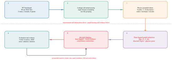
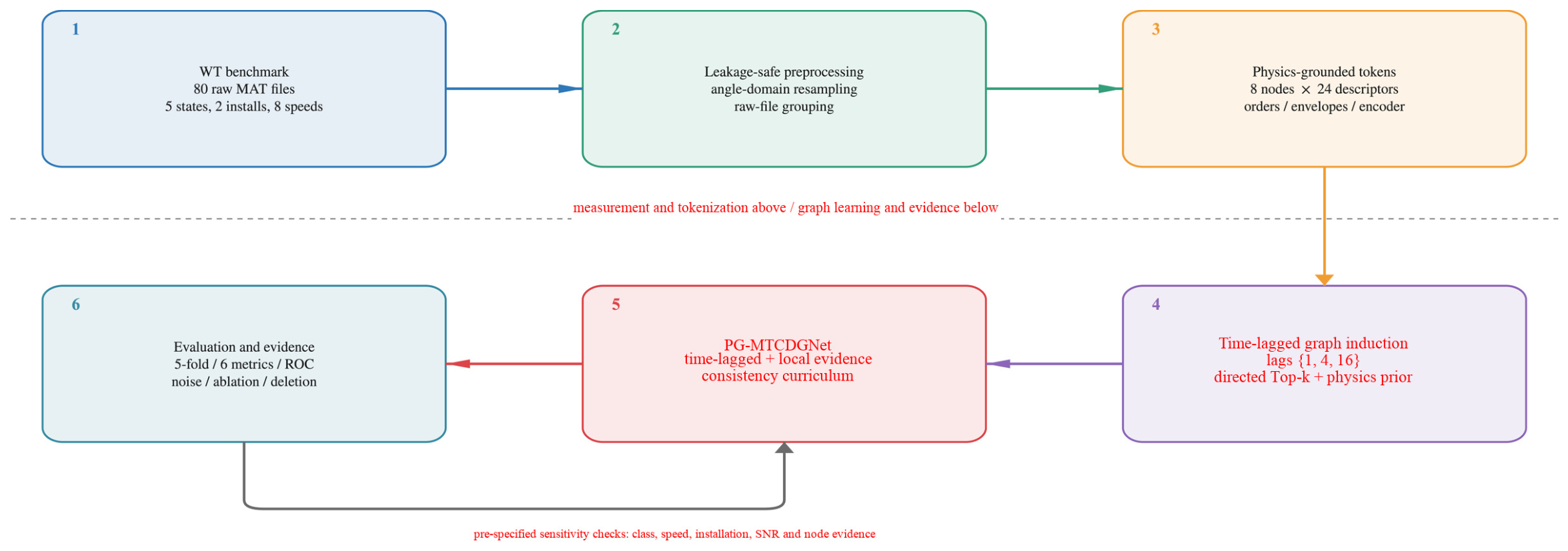
Figure 1 summarizes the workflow. Leakage-controlled equal-angle preprocessing produces the physical nodes, after which multi-lag predictive correlations induce a directed graph for each sample. The noise curriculum, graph propagation, and dual-evidence fusion are fitted only on the training files. Statistics estimated from a training fold are then frozen and applied to its held-out files. Evaluation covers classification performance, perturbation robustness, and the structured evidence outputs produced by the model.

Figure 1. End-to-end workflow for PG−MTCDGNet development and evaluation.

2.3. Phase-Synchronous Resampling and Eight-Node Construction

We let f_r(t) denote the instantaneous rotational frequency estimated from the encoder. Its integral defines the rotational phase. Interpolation at 1024 equally spaced positions per revolution maps the frequency components that move with speed to approximately stationary orders.

$$\theta (t)=2\pi {\int }_0^t{f}_r(u)du,\overline{x}[n]=x\left(t\left({\theta }_n\right)\right)$$

(2)

To limit the graph size, each angle-domain waveform is phase-uniformly downsampled to T = 256. The eight nodes are the X-order waveform, X-transient, Y-order waveform, Y-transient, X-envelope, Y-envelope, pointwise XY-interaction, and encoder micro-speed. Each node contains 12 sequence descriptors and 12 physical tags allocated from a 96-dimensional physical feature vector.Table 1 lists the signal sources and physical interpretations of the eight nodes.

$${\mathbf{H}}_i=[{\mathbf{h}}_{i,1};\dots ;{\mathbf{h}}_{i,8}]\in R^{8\times 24},{\mathbf{h}}_{i,v}=\left[\varphi \right({\mathbf{z}}_{i,v})\Vert {\psi }_{i,v}]$$

(3)

Table 1. Eight physics-grounded graph nodes.

Node	Signal Source	Primary Physical Interpretation
X-order	Equal-angle X waveform	Mesh and order response
X-transient	High-pass X residual	Localized impact and crack transient
Y-order	Equal-angle Y waveform	Orthogonal transmission path
Y-transient	High-pass Y residual	Orthogonal transient impact
X-envelope	Hilbert envelope of X	Modulation and local energy
Y-envelope	Hilbert envelope of Y	Transmission-path modulation
XY-interaction	Pointwise X × Y product	Cross-channel coupling
Encoder-speed	Encoder micro-speed	Speed perturbation and torsional variation

2.4. Multi-Scale Time-Lagged Directed Graph

At T = 256 angle samples per revolution, the lags of 1, 4, and 16 samples correspond to approximately 1.4°, 5.6°, and 22.5° of shaft rotation. This geometrically spaced set separates immediate sample-to-sample transmission, an intermediate local-impact neighborhood, and slower modulation without expanding the graph bank excessively. For each ordered pair of a source node u and target node v, the past-to-future correlation is evaluated at these three lags. The edge matrix follows the convention that row v and column u store u → v. Absolute correlation measures predictive strength; direction follows from the ordering of the lagged indices. The lag set was fixed for every fold and was not re-selected on held-out data.

$$r_{u\to v}^{\left(\tau \right)}\left(i\right)=\left|corr\left({\mathit{z}}_{i,u}[1:T-\tau ],{\mathit{z}}_{i,v}[1+\tau :T]\right)\right|,\tau \in \{1,4,16\}$$

(4)

$$r_{u\to v}^{¯}(i)=\underset{\tau \in \{1,4,16\}}{\max }{r}_{u\to v}^{(\tau )}(i)$$

(5)

Each receiving node retains only its three strongest data-driven incoming edges, in addition to a self-loop. With eight nodes, k = 3 retains three of the seven possible non-self parents per target (24 data-driven incoming edges per sample at most), enforcing a sparse and inspectable graph while avoiding single-parent dependence. The same k was used in every fold; no fold-specific tuning was performed.

2.5. Label-Independent Physical Prior and Normalization

The physical prior describes transmission mechanisms only and contains no health-state information. Prior links connect the orthogonal channels, transients to their envelopes, the XY-interaction to both envelopes, and the encoder speed to the vibration and envelope nodes. If a physically plausible edge is absent from the data-driven top-k set or is weaker than the floor, it receives a weight of 0.35 before row normalization. This floor does not overwrite a stronger learned correlation; after normalization, its effective contribution depends on the other incoming weights. The value was fixed across folds rather than optimized on held-out performance.

$$\widetilde{A_{vu}}(i)=max\left(r_{u\to v}^{¯}\left(i\right)I_{u\in TopK\left(v\right)},0.35{\Pi }_{vu}\right)+I_{u=v},A_{vu}(i)={\displaystyle \frac{\widetilde{A_{vu}}\left(i\right)}{\sum _j\widetilde{A_{vj}}(i)+\epsilon }}$$

(6)

The time-lagged graph in PG-MTCDGNet encodes a correlation-based past-to-future predictive association under stated mechanical constraints. It is not an intervention model, and its adjacency should not be interpreted as a validated physical transmission law or a verified explanation.

2.6. Graph Shrinkage and Multi-Hop Graph Filtering

Under strong perturbation, standardized node features are first clipped to [−6, 6]. The representation then combines the node itself, its one-hop parents, and its two-hop parents. The fixed convex weights prevent the representation from depending exclusively on neighbors and thereby limit oversmoothing.

$${\mathbf{H}}_c=0.55clip\left(\mathbf{H}\right)+0.30\mathbf{A}clip\left(\mathbf{H}\right)+0.15{\mathbf{A}}^{2}clip\left(\mathbf{H}\right)$$

(7)

The graph branch forms a filter bank from zero-hop, one-hop, two-hop, and directional-flux blocks. Mean and maximum pooling are applied to every block. Directional flux compares propagation through A with propagation through its transpose, retaining information that would disappear in a symmetric graph.

$${\mathbf{G}}_1=\mathbf{A}{\mathbf{H}}_c,{\mathbf{G}}_2={\mathbf{A}}^2{\mathbf{H}}_c,{\mathbf{G}}_{\Delta }=\mathbf{A}{\mathbf{H}}_c-{\mathbf{A}}^{\mathsf{\top }}{\mathbf{H}}_c$$

(8)

$${\mathbf{q}}_c=Concat\left(vec\left({\mathit{H}}_c\right),\left\{MeanPool\right(\mathit{B}),MaxPool(\mathit{B}){\}}_{\mathit{B}\in \{{\mathit{H}}_c,{\mathit{G}}_1,{\mathit{G}}_2,{\mathit{G}}_{\Delta }\}}\right)$$

(9)

2.7. Dual-Evidence Posterior Fusion

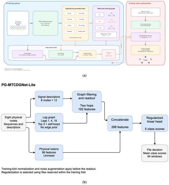
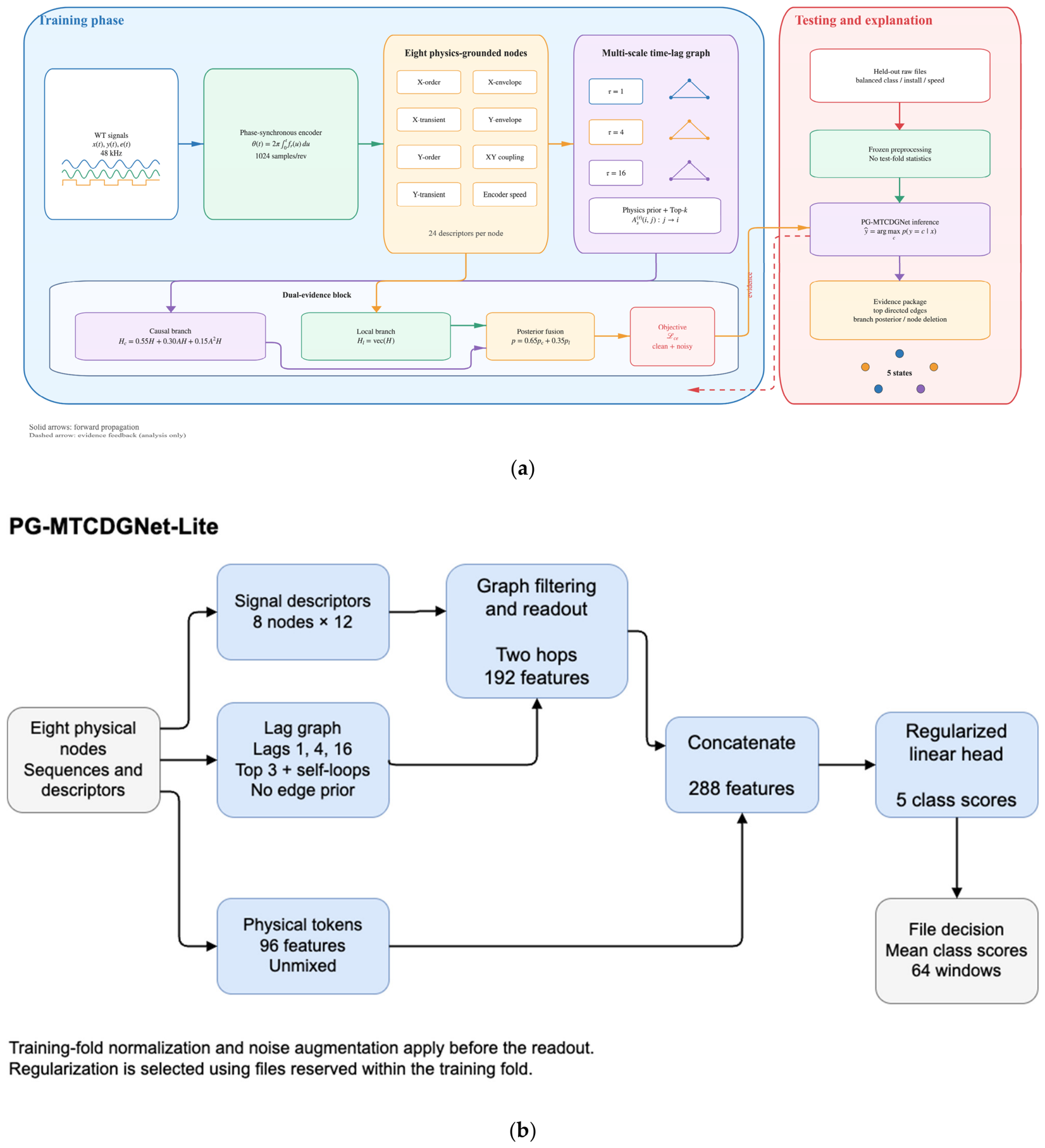
Graph shrinkage can attenuate isolated peaks, so an unsmoothed local branch is trained in parallel. The graph branch uses hidden layers of 160 and 96 units to produce the graph posterior, while the local branch applies hidden layers of 96 and 64 units directly to the vectorized node matrix. The two branches are optimized separately and combined at the posterior level, which allows their contributions to be compared independently. Figure 2a illustrates the original dual-branch architecture; it is presented alongside Figure 2b.

$${\mathbf{q}}_l=vec\left(\mathbf{H}\right),{\mathbf{p}}_c=softmax\left(f_c\right({\mathbf{q}}_c\left)\right),{\mathbf{p}}_l=softmax\left(f_l\right({\mathbf{q}}_l\left)\right)$$

(10)

$$\mathbf{p}=0.65{\mathbf{p}}_c+0.35{\mathbf{p}}_l,\widehat{c}=arg\underset{k}{\max }{p}_k$$

(11)

Figure 2. PG-MTCDGNet architecture for training, inference, and evidence reporting as in (a). The original dual-branch configuration is shown alongside the depth-reduced variant in (b).

2.8. Noise-Consistency Curriculum and Objective

During training, standardized node features are perturbed with Gaussian noise at −6, 0, 6, and 10 dB and are learned jointly with the clean examples. The held-out fold contributes neither normalization statistics nor graph or network parameters. The perturbation variance is computed from the feature power of each sample.

$${\tilde{\mathbf{H}}}^{\left(\gamma \right)}=\mathbf{H}+ϵ,ϵ\sim N(0,{\sigma }_{\gamma }^2\mathbf{I}),{\sigma }_{\gamma }^2={\displaystyle \frac{\Vert \mathit{H}{\Vert }_F^2/\left(8d\right)}{10^{\gamma /10}}}$$

(12)

The implemented loss is supervised cross-entropy over clean and noisy versions; no explicit KL penalty is optimized. The infinity symbol in Equation (13) denotes the clean version.

$$L={\displaystyle \frac{1}{5\left|B\right|}}\sum _{i\in B}\sum _{\gamma \in \Gamma \cup \{\infty \}}-\log p_{i,c_i}^{\left(\gamma \right)}$$

(13)

2.9. Training and Inference Procedure

The implementation is summarized below as mathematical mappings and reproducible operations rather than software-specific pseudocode.

• We specify the grouped raw-file dataset, lag set T = {1, 4, 16}, k = 3, physical-prior matrix Π, noise curriculum Γ = {−6, 0, 6, 10} dB, and five file folds.
• For fold q, we use file identifiers to define the training and test indices. We estimate each normalization statistic from the training files and apply the frozen statistics to the held-out files.
• For each window, we perform encoder-based phase synchronization and construct the eight-node sequences and the 8 × 24 feature matrix.
• At each lag, we compute the ordered predictive correlations, retain the top-k incoming edges, add the label-independent physical prior, and row-normalize the adjacency.
• We generate perturbed copies only for the training fold. The graph branch applies graph shrinkage and multi-hop filtering; the local branch preserves the unsmoothed node evidence.
• We optimize the two classification heads, combine their posteriors with fixed weights, and we then compute the six classification metrics and one-versus-rest AUC on the held-out files.
• We set each node to zero in turn and record the changes in accuracy, macro-F1, and class recall; we then export the lag-specific directed edges and their asymmetry indices.

$$I_{te}^{\left(q\right)}=\{i:g_i\in F_q\},I_{tr}^{\left(q\right)}=\{1,\dots ,N\}\setminus I_{te}^{\left(q\right)}$$

(14)

2.10. Experimental Protocol

2.10.1. Dataset and Implementation

Table 2 summarizes the dataset and implementation settings. Each raw file contributes 64 windows. Grouping by file rather than randomly splitting windows prevents adjacent segments of the same continuous record from entering both the training and test sets. Each model uses the same folds, training-fold normalization, and class order.

Table 2. Dataset and implementation settings.

Item	Setting
Health states	Healthy, wear, root crack, broken tooth, missing tooth
Sensor installations	2
Input speeds	20, 25, 30, 35, 40, 45, 50, and 55 Hz
Channels	X vibration, Y vibration, encoder
Sampling rate	48 kHz
Raw files/windows	80/5120
Five-fold rule	MAT-file isolation; balanced by class, installation, and speed
Random seed	20260730 for the primary split and visualization
Software	MATLAB R2025b

Computations were performed on an Apple M3 Max workstation with a 16-core CPU and 48 GB unified memory under macOS. MATLAB R2025b was used for signal preprocessing and the neural baseline experiments; the Lite ridge-regression experiments used Python with NumPy, SciPy, and scikit-learn.

2.10.2. Baselines

The ESC-DGCN-style entry is an in-house common-input architecture control. It uses the same eight-node descriptors, file splits, training-fold normalization, and class labels; under the matched curriculum it also receives the same perturbed training samples and optimization budget. As specified in Table 3, this implementation uses a symmetric dynamic graph, multi-hop filtering, and a 64/96-unit head.

Table 3. Baselines and unified implementation settings.

Model	Category	Configuration
Random Forest	Classical machine learning	160 bagged trees; at most 63 splits
SAE-MLP	Deep learning	96-dimensional sparse autoencoder; 64/32-unit MLP
Deep MLP	Deep learning	128/64 hidden units; L2 regularization
ESC-DGCN-style control	Controlled reference implementation	Symmetric dynamic graph; multi-hop filtering; 64/96 head
PG-MTCDGNet	Proposed method	Multi-lag directed graph; dual evidence; noise curriculum

2.10.3. Metrics

The five-class task is evaluated using accuracy, macro-averaged sensitivity, specificity, precision, $F1$, and Jaccard index. We let $T{P}_k$, $F{P}_k$, $T{N}_k$, and $F{N}_k$ denote the one-versus-rest counts for class k.

$$Acc={\displaystyle \frac{\sum _{k}T{P}_k}{N}},Sen={\displaystyle \frac{1}{K}}\sum _k{\displaystyle \frac{T{P}_k}{T{P}_k+F{N}_k}},Spe={\displaystyle \frac{1}{K}}\sum _k{\displaystyle \frac{T{N}_k}{T{N}_k+F{P}_k}}$$

(15)

$$Pre={\displaystyle \frac{1}{K}}\sum _k{\displaystyle \frac{T{P}_k}{T{P}_k+F{P}_k}},F1={\displaystyle \frac{1}{K}}\sum _k{\displaystyle \frac{2P_k{R}_k}{P_k+R_k}},Jac={\displaystyle \frac{1}{K}}\sum _k{\displaystyle \frac{T{P}_k}{T{P}_k+F{P}_k+F{N}_k}}$$

(16)

Macro-AUC is the arithmetic mean of the five one-versus-rest ROC areas. Tables report the mean and sample standard deviation over five folds. Confusion matrices pool all out-of-fold predictions.

2.10.4. Noise Controls and Structured Evidence Protocol

The default noise experiment compares the complete training configuration of each method; only PG-MTCDGNet includes the consistency curriculum in that comparison. To separate training information from graph structure, a matched-curriculum control supplies deep MLP, ESC-DGCN, and PG-MTCDGNet with the same perturbed training samples, hidden widths, and optimization budget. Noise is added after fold-specific standardization in node-feature space. These experiments characterize classifier robustness to feature-chain perturbation; they do not show that graph structure itself creates the robustness gain or simulate raw sensor noise.

Structured evidence outputs are summarized at three levels: mean and dispersion of directed edges at each lag, out-of-fold performance of the local, graph, and fused branches, and the decline in macro-F1 and class recall after setting one node to zero. These summaries show what the model reports, but they are not expert validation or physical verification of an explanation.

$$\eta (\mathbf{A})={\displaystyle \frac{\Vert \mathit{A}-{\mathit{A}}^{\mathsf{\top }}{\Vert }_F}{\Vert \mathit{A}+{\mathit{A}}^{\mathsf{\top }}{\Vert }_F+\epsilon }}$$

(17)

2.10.5. Held-out-Condition Validation

Two installation-holdout tests trained on all 40 raw files from one sensor installation and evaluated all 40 files from the other. Four speed-holdout tests each excluded one predefined adjacent speed pair (20–25, 30–35, 40–45, or 50–55 Hz), leaving 60 files for training and 20 for testing. Every file contributed 64 windows. Normalization was estimated from training files only. The MLP, a capacity-control dual MLP, the controlled dynamic-graph reference, PG-MTCDGNet, and its structural ablations received identical training-file noise realizations at −6, 0, 6, and 10 dB with clean examples. Network widths, iteration limits, graph settings, and the 0.65 fusion weight were fixed before testing. At inference, graph adjacency was constructed from the individual test window without its label. We report window metrics and file metrics obtained by averaging the 64 window posteriors within each raw file. Additional test noise was injected after feature extraction while the adjacency was held fixed; it is a feature perturbation test and not a raw-sensor-noise test.

2.10.6. Depth-Reduced PG-MTCDGNet-Lite

PG-MTCDGNet-Lite retains the eight nodes and directed top-three adjacency obtained from the maximum lagged correlation over lags of 1, 4, and 16. Self-loops and row normalization are retained, but the fixed edge-prior floor is removed. Each node’s first 12 descriptors have the same signal-statistical meaning across nodes; its remaining 12 entries belong to different physical-token groups. The Lite variant propagates only the comparable signal descriptors and retains all 96 physical tokens in a separate readout. This separation avoids averaging unlike physical quantities along a shared feature coordinate.

We let S denote the standardized and clipped eight-by-twelve signal-descriptor matrix and A the directed adjacency. The fixed two-hop filter is

$$G=0.55S+0.30AS+0.15A^{2}S$$

The readout concatenates the flattened G with the nodewise mean and maximum of G, its one- and two-hop propagated forms, and forward-minus-reverse one-hop propagation. These 192 graph features are concatenated with the 96 unmixed physical tokens. The resulting 288 features are standardized using the augmented training set. A single regularized linear head replaces the two nonlinear classifiers and posterior fusion. With one-hot target matrix Y and design matrix X, its objective is

$$\underset{W,b}{\mathrm{m}\mathrm{i}\mathrm{n}}{\displaystyle \frac{1}{N}}{\Vert XW+1b^{\mathrm{T}}-Y\Vert }_{\mathrm{F}}^2+\lambda {\Vert W\Vert }_{\mathrm{F}}^2$$

The intercept is unpenalized. Regularization is selected from 0.001, 0.01, 0.1, 1, and 10 using the two lowest available speeds reserved within each outer training fold. The other training files fit each candidate; selection first maximizes the mean file accuracy over clean, −6, 0, and 6 dB conditions followed by macro-F1, with the remaining ties resolved by grid order. The chosen value is 0.1 for the 30–35 Hz outer holdout and 0.001 for the other five folds. The final head is refitted on all outer training files. Clean data and four Gaussian feature-noise copies at −6, 0, 6, and 10 dB are used for fitting. All Lite ablations use the same training realizations and selection procedure. The strong MLP reference is retained with its original settings and the identical held-out feature perturbations. The primary file decision averages 64 class-score vectors before taking the largest score; linear-head scores are not interpreted as calibrated probabilities.

The primary summary averages the four test conditions within each fold, then averages the two installation folds and the four speed folds separately, assigning each shift family a weight of one half. Window metrics are secondary. Architecture development and evaluation used the same 80 recordings across successive comparisons; these estimates are therefore exploratory despite training-fold regularization selection.

3. Results

3.1. Five-Fold Diagnostic Performance

Table 4 reports the six classification metrics. PG-MTCDGNet achieved 99.61% ± 0.33% accuracy, 99.63% ± 0.31% macro-F1, and 0.99999 macro-AUC. Deep MLP remained the strongest clean-data classifier at 99.75%, 0.14 percentage points above PG-MTCDGNet. The clean-data scores are therefore descriptive and are not evidence that the graph improves accuracy. The ESC-DGCN entry is a controlled reference implementation rather than the published code, so it is not used to support a claim about the published model.

Table 4. Six classification metrics under raw-file-isolated five-fold validation (%, mean ± standard deviation).

Model	Accuracy	Sensitivity	Specificity	Precision	Macro-F1	Jaccard
Random Forest	95.21 ± 4.47	95.74 ± 3.66	98.82 ± 1.10	95.49 ± 3.84	95.27 ± 4.36	91.56 ± 7.05
SAE-MLP	97.56 ± 0.96	97.57 ± 1.08	99.39 ± 0.24	97.58 ± 0.91	97.54 ± 1.03	95.25 ± 1.96
Deep MLP	99.75 ± 0.28	99.79 ± 0.23	99.94 ± 0.07	99.74 ± 0.28	99.76 ± 0.26	99.53 ± 0.51
ESC-DGCN-style control	99.36 ± 0.74	99.46 ± 0.59	99.84 ± 0.18	99.36 ± 0.72	99.39 ± 0.68	98.82 ± 1.30
PG-MTCDGNet	99.61 ± 0.33	99.66 ± 0.27	99.90 ± 0.08	99.60 ± 0.33	99.63 ± 0.31	99.26 ± 0.60

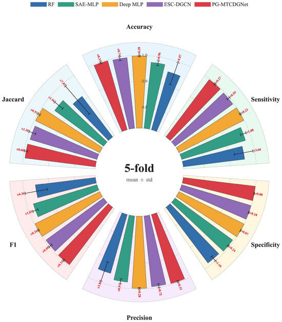
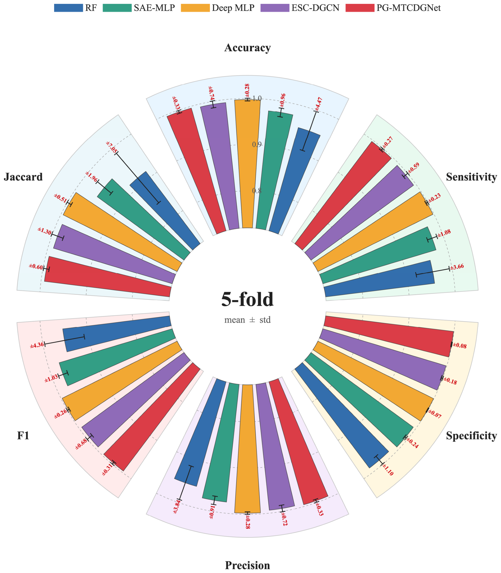
Figure 3 summarizes the six metrics and their fold-to-fold dispersion. PG-MTCDGNet was close to the upper bound for specificity and AUC, and its variability was substantially lower than that of the random forest and ESC-DGCN. Balancing each fold by class, installation, and speed limited the influence of an unusually difficult condition on the aggregate result.

Figure 3. Six-metric comparison across five raw-file-isolated folds (mean ± standard deviation).

Across all 5120 out-of-fold decisions, random forest, SAE-MLP, deep MLP, the ESC-DGCN-style controlled reference, and PG-MTCDGNet made 245, 125, 13, 33, and 20 errors, respectively. These counts describe the supplied implementations under a common protocol; because the ESC-DGCN entry is not the published authors’ code, the difference is not interpreted as a reduction relative to published ESC-DGCN. Reporting counts remains useful in this near-saturated regime because small percentage-point changes correspond to a few decisions.

$$RE{R}_{a\to b}={\displaystyle \frac{E_a-E_b}{E_a}}\times 100\%,RE{R}_{ESC\to PG}={\displaystyle \frac{33-20}{33}}\times 100\%=39.39\%$$

(18)

Table 5 presents fold-specific accuracies and error counts.PG-MTCDGNet obtained fold accuracies of 100%, 99.80%, 99.61%, 99.51%, and 99.12%; its least favorable fold therefore remained above 99%. ESC-DGCN fell to 98.14% in Fold 4, which increased its standard deviation. The accuracy coefficient of variation was 0.33% for PG-MTCDGNet, compared with 0.28% for deep MLP, 0.74% for ESC-DGCN, 0.98% for SAE-MLP, and 4.69% for random forest. The dual-evidence model did not obtain its mean from one unusually easy fold.

Table 5. Fold-specific accuracy, total out-of-fold errors, and coefficient of variation.

Model	Fold 1	Fold 2	Fold 3	Fold 4	Fold 5	Errors	CV (%)
Random Forest	98.73	94.82	87.70	98.14	96.68	245	4.69
SAE-MLP	96.48	96.68	97.75	98.14	98.73	125	0.98
Deep MLP	100	99.90	99.90	99.61	99.32	13	0.28
ESC-DGCN-style control	100	99.41	99.90	98.14	99.32	33	0.74
PG-MTCDGNet	100	99.80	99.61	99.51	99.12	20	0.33

The paired fold-wise accuracy differences between PG-MTCDGNet and the ESC-DGCN-style controlled reference were 0, 0.39, −0.29, 1.37, and −0.20 percentage points. With only five folds, the mean difference of 0.25 percentage points had an approximate 95% paired confidence interval from −0.58 to 1.09 percentage points. Because this interval includes zero, the data do not establish statistical superiority, even within this controlled reference comparison. The defensible interpretation is narrower: PG-MTCDGNet produced a similar high clean-data score while exposing a different structured evidence representation.

$${\Delta }_q=Ac{c}_{PG}^{\left(q\right)}-Ac{c}_{ESC}^{\left(q\right)},\overline{\Delta }=0.25\%,C{I}_{95\%}=[-0.58,1.09]\%$$

(19)

Near-perfect accuracy also limits statistical power because each fold contains roughly ten or fewer errors and changing one prediction moves fold accuracy by about 0.10 percentage points. Mean differences, intervals, and error counts should therefore be interpreted together. The synchronized improvements in macro sensitivity, precision, F1, and Jaccard indicate that the result was not produced by favoring one class. A specificity of 99.90% further shows that the model did not obtain high recall by systematically over-predicting a fault category.

3.2. Confusion Patterns, Discriminant Space, and ROC Analysis

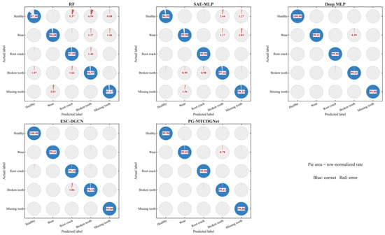
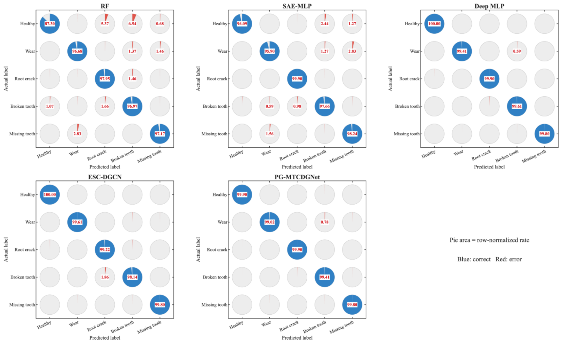
Figure 4 pools out-of-fold predictions into row-normalized pie-matrix confusion plots. PG-MTCDGNet attained recalls of approximately 99.90%, 99.02%, 99.90%, 99.41%, and 99.80% for healthy, wear, root crack, broken tooth, and missing tooth, respectively. The remaining mistakes were concentrated among wear, root crack, and broken tooth, which share partially overlapping impact and modulation signatures. Wear can produce distributed surface roughness and broadband envelope modulation, whereas a broken tooth produces more phase-localized impacts; after window-level peak, spectral, envelope, and energy descriptors are aggregated, severe wear and weak broken-tooth windows can occupy adjacent score neighborhoods under some speeds and transfer paths. This is a descriptive interpretation of feature-space overlap; t-SNE does not identify a mechanism. Relative to ESC-DGCN, recall increased by about 0.7 and 1.3 percentage points for root crack and broken tooth, whereas healthy and wear were lower by about 0.1 and 0.6 points and missing tooth was nearly unchanged.

Figure 4. Pie-matrix confusion plots assembled from out-of-fold predictions for the five models.

The baseline patterns help locate the source of difficulty. Random forest recalled only about 87.3% of healthy cases, suggesting that aggregate statistics were sensitive to installation- or speed-dependent amplitude changes. SAE-MLP increased healthy recall to 96.1% but retained visible confusion for wear and missing tooth. Deep MLP produced an almost perfectly diagonal matrix, confirming that the 24-dimensional node descriptors were already highly discriminative. The role of PG-MTCDGNet is therefore not to replace all dense classifiers; it is to retain comparable clean-data performance while exposing lagged edges, physical nodes, and branch posteriors that a conventional MLP does not provide.

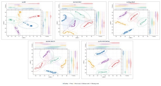
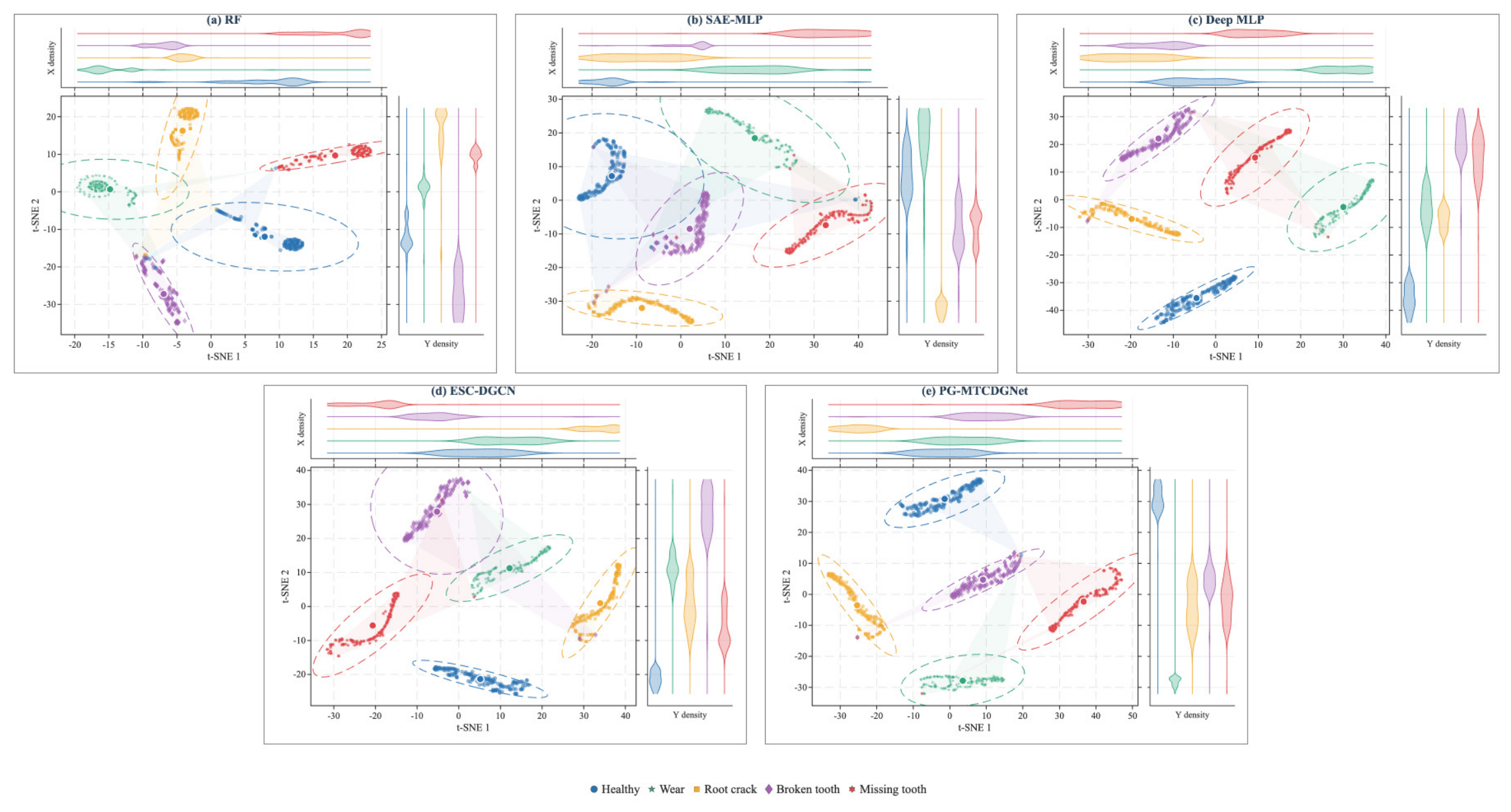
Figure 5 applies t-SNE to a common five-dimensional out-of-fold discriminant-score space instead of comparing hidden layers of different dimensionality. The projections include class boundaries, 95% covariance ellipses, centroids, and marginal kernel-density ridges. Random forest and SAE-MLP formed elongated manifolds with overlapping marginal densities, consistent with residual installation and speed subgroups. Deep MLP, ESC-DGCN, and PG-MTCDGNet formed tighter clusters. In PG-MTCDGNet, healthy, root crack, and missing tooth were distinctly separated, whereas wear and broken tooth remained close but distinguishable, consistent with the related modulation and impact descriptors discussed for Figure 4. Their t-SNE proximity is qualitative and does not establish a shared physical mechanism.

Figure 5. t-SNE projections of common out-of-fold discriminant scores with marginal density estimates.

t-SNE preserves local neighborhoods rather than global Euclidean distances, and changes in random seed can rotate or mirror a projection. We fixed the sample set, seed, and perplexity and use Figure 5 only as a qualitative check of local cluster consistency. Performance claims rest on out-of-fold metrics, ROC curves, and file-level errors.

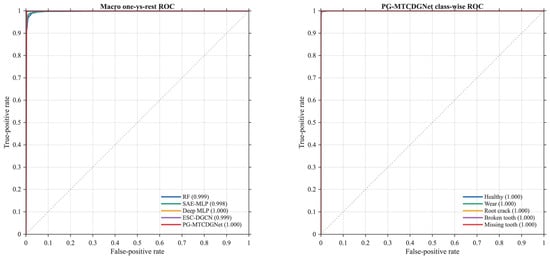
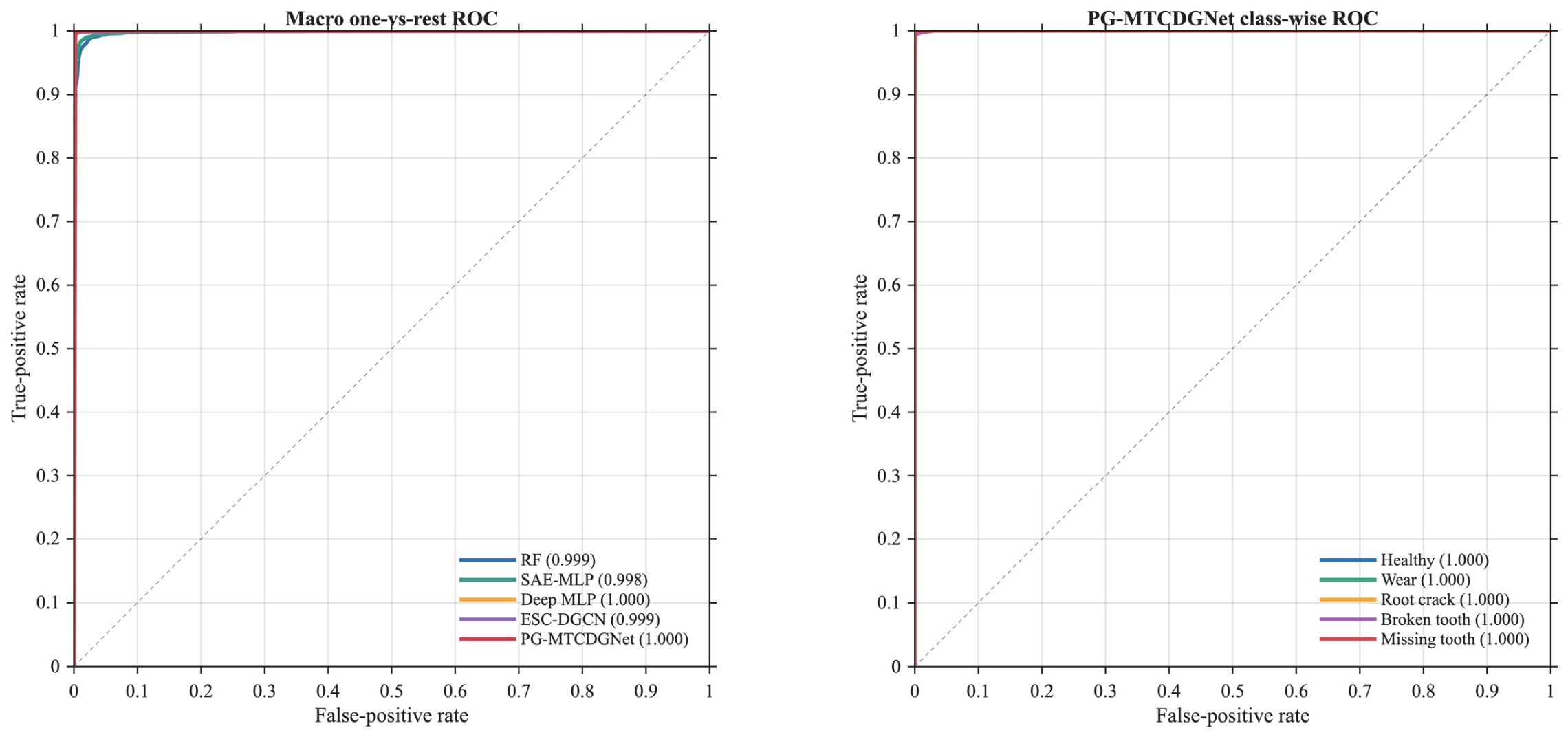
Figure 6 shows the macro-average ROC and the class-wise curves of PG-MTCDGNet. Macro-AUC was 0.99999; broken tooth had the lowest class-wise AUC but remained close to 0.998. A few samples can therefore be misclassified at the maximum-posterior decision while their true-class scores still rank above most negative examples. Threshold adjustment could prioritize crack or broken-tooth sensitivity without retraining the model. AUC close to one does not establish probability calibration, which requires a separate calibration set.

$$AU{C}_{macro}={\displaystyle \frac{1}{K}}{{\displaystyle \sum _{k=1}^K}{\int }_0^{1}TPR}_k(FPR)dFPR,K=5$$

(20)

Figure 6. Macro−average and class-wise ROC curves for PG-MTCDGNet.

3.3. Training Behavior

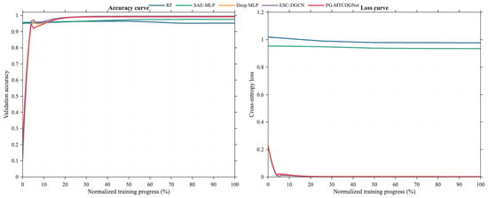
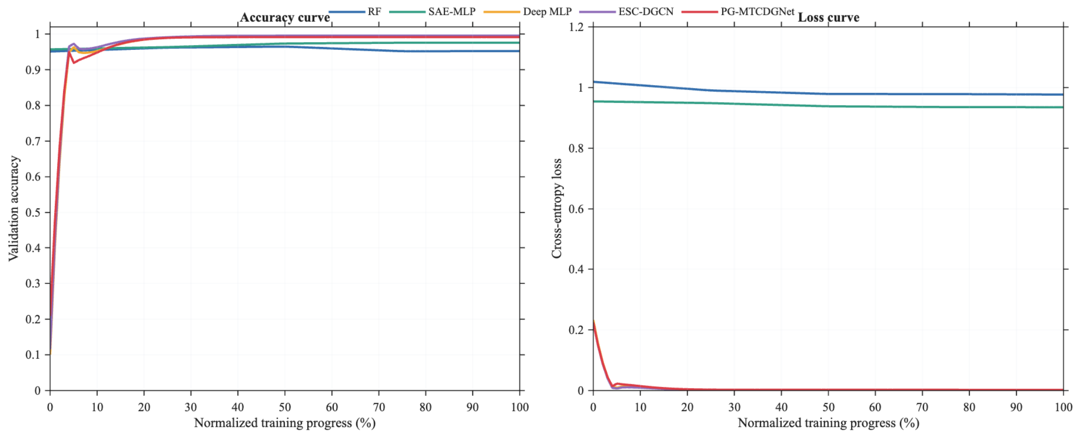
Figure 7 places all learning histories on a normalized training-progress axis. Deep MLP, ESC-DGCN, and PG-MTCDGNet converged rapidly during the first 20% of optimization. The random forest and SAE-MLP traces are genuine learning curves obtained by progressively increasing the training subset, so their horizontal axes are not epoch-by-epoch gradient trajectories. The figure is used to assess convergence shape and overfitting, not the absolute training speed.

Figure 7. Accuracy and loss/learning-progress curves for the five models.

PG-MTCDGNet reached a stable validation plateau without a sustained late-stage loss increase. ESC-DGCN also converged quickly but showed more visible terminal variation, consistent with its drop in Fold 4. The local branch can exploit an isolated physical cue early in training; the graph branch then adds cross-node dependencies. Running the two branches in parallel prevents an erroneous adjacency from controlling the complete representation. With eight nodes, three lags, and k = 3, each sample retains, at most, 24 data-driven incoming edges plus a small number of prior links, which remains directly inspectable.

3.4. Robustness Under the Default Training Configurations

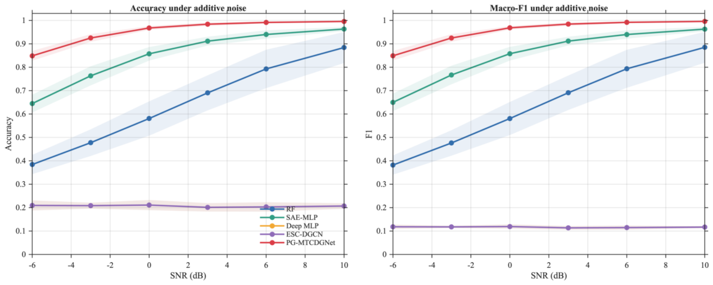
PG-MTCDGNet achieved 84.86%, 96.78%, and 99.57% accuracy at −6, 0, and 10 dB, respectively. These values describe the complete configuration—graph branch, local branch, posterior fusion, and noise-consistency curriculum—and cannot be assigned to the directed graph alone. The matched-curriculum control below is the relevant comparison for separating training from architecture.

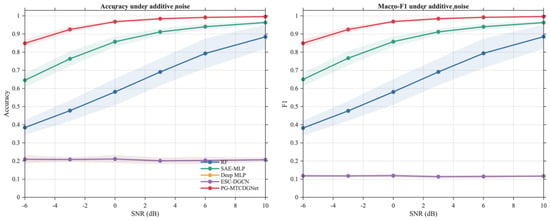
Table 6 reports noise-level accuracies; Figure 8 shows accuracy and macro-F1 across the tested feature-noise levels. PG-MTCDGNet improved monotonically from 84.86% accuracy at −6 dB to 92.50%, 96.78%, 98.40%, 99.14%, and 99.57% at −3, 0, 3, 6, and 10 dB. Its average accuracy over the six noise levels was 95.21%, compared with 84.67% for SAE-MLP and 63.50% for random forest. Deep MLP and ESC-DGCN, which had seen only clean features during default training, averaged about 20.66% and approached random performance. This comparison answers how complete deployable configurations behave after an unanticipated feature perturbation; it does not establish that dense or undirected architectures are intrinsically unable to learn noise robustness.

$$R{A}_{\Gamma }={\displaystyle \frac{1}{\left|\Gamma \right|}}\sum _{\gamma \in \Gamma }Acc(\gamma ),\Gamma =\{-6,-3,0,3,6,10\}dB$$

(21)

Table 6. Accuracy under additive feature noise using each method’s default training configuration (%, five-fold mean).

Model	−6 dB	0 dB	6 dB	10 dB
Random Forest	38.42	58.09	79.28	88.42
SAE-MLP	64.47	85.74	94.00	96.33
Deep MLP	20.94	21.09	20.29	20.68
ESC-DGCN-style control	20.94	21.09	20.29	20.68
PG-MTCDGNet	84.86	96.78	99.14	99.57

Figure 8. Accuracy and macro−F1 under additive feature noise using each model’s default training configuration.

3.5. Matched-Curriculum Control

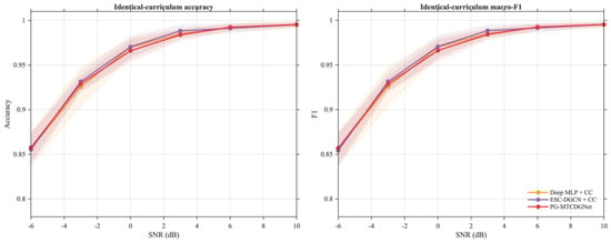
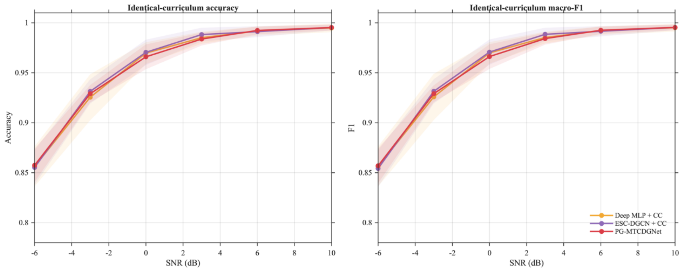
Once deep MLP + CC and the ESC-DGCN-style controlled reference + CC received the same noisy training examples, the difference from PG-MTCDGNet narrowed sharply. At −6 dB, accuracies were 85.62%, 85.53%, and 85.74% for deep MLP + CC, the ESC-DGCN-style controlled reference + CC, and PG-MTCDGNet, respectively. At 0 dB, the corresponding values were 96.97%, 97.05%, and 96.60%. Averaged over six SNRs, the three models attained 95.39%, 95.53%, and 95.40%, with a maximum difference of only 0.14 percentage points.

Table 7 and Figure 9 compare the deep models under the matched noise curriculum. The matched-curriculum control shows that the dominant robustness gain comes from consistency training rather than graph topology. Deep MLP, ESC-DGCN + CC, and PG-MTCDGNet were effectively tied across the six SNRs, with a maximum difference of only 0.14 percentage points. A dense MLP is therefore sufficient when only closed-set accuracy and minimal computation are required. PG-MTCDGNet is useful only for the additional structured outputs—lag-specific propagation, branch posteriors, and node-occlusion responses—and not because the graph has been shown to improve robustness.

Table 7. Accuracy under an identical noise-consistency curriculum (%, five-fold mean).

Model	−6 dB	0 dB	6 dB	10 dB
Deep MLP + CC	85.62	96.97	99.18	99.49
ESC-DGCN-style control + CC	85.53	97.05	99.12	99.53
PG-MTCDGNet	85.74	96.60	99.24	99.53

Figure 9. Robustness comparison when the three deep models receive the same noise–consistency curriculum.

3.6. Ablation Study

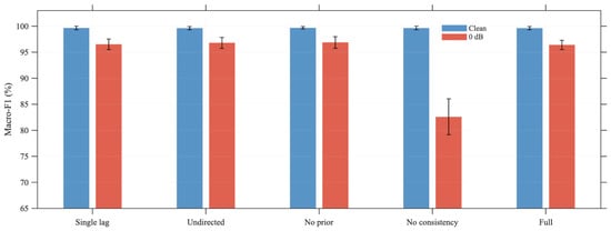
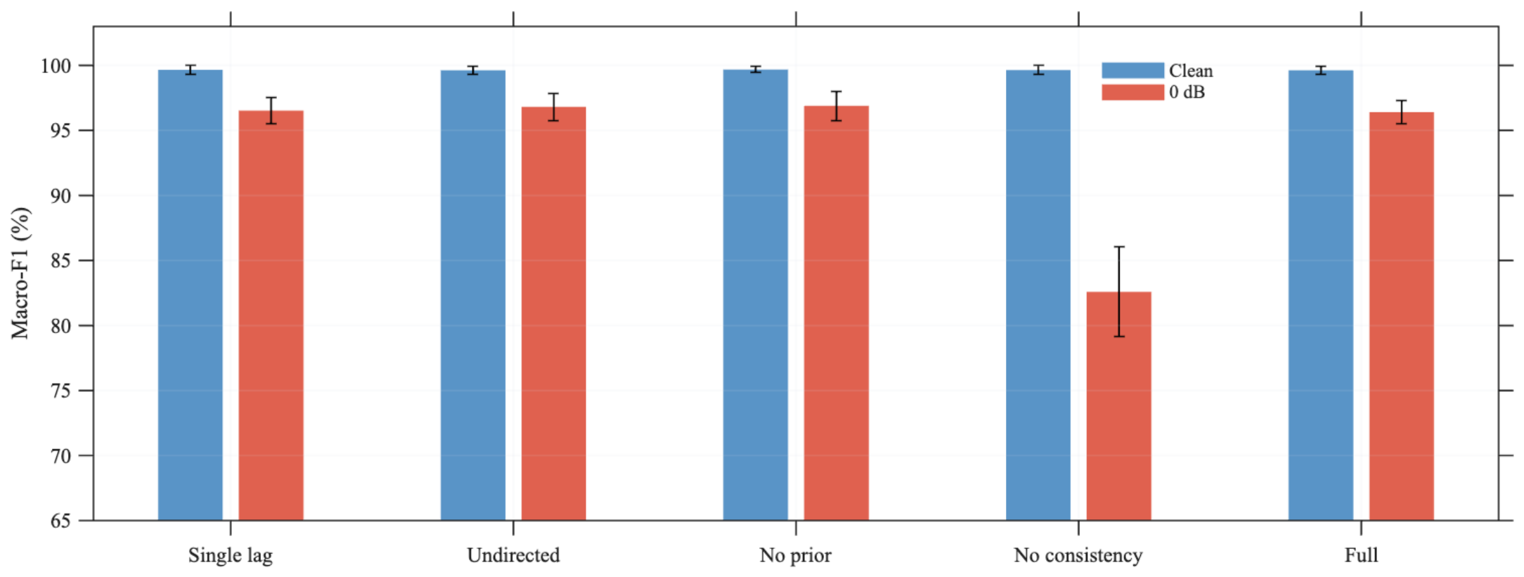
Table 8 and Figure 10 summarize the component ablations on clean and 0 dB inputs. Removing the consistency curriculum left the clean macro-F1 near 99.65% but reduced 0 dB macro-F1 to 82.58%. In contrast, removing multi-scale lags, edge direction, or the physical prior changed 0 dB macro-F1 by less than one percentage point, and each simplified variant was slightly higher than the complete model on this benchmark. Their accuracy benefit was not consistent across conditions. Their demonstrated role is to constrain the representation and produce structured evidence outputs; the curriculum, not the graph, controls the robustness ceiling.

Table 8. Component ablation measured by macro-F1 (%, five-fold mean ± standard deviation).

Variant	Clean	0 dB
Without multi-scale lags	99.66 ± 0.32	96.53 ± 1.03
Without edge direction	99.63 ± 0.31	96.82 ± 1.04
Without physical prior	99.68 ± 0.25	96.89 ± 1.11
Without consistency curriculum	99.65 ± 0.36	82.58 ± 3.44
Complete PG-MTCDGNet	99.63 ± 0.31	96.40 ± 0.91

Figure 10. Component ablation on clean and 0 dB inputs.

The full model attained 96.40% macro-F1 at 0 dB. Removing multi-scale lags, direction, and the physical prior yielded 96.53%, 96.82%, and 96.89%, respectively. The 24-dimensional node descriptors and the consistency curriculum were already highly discriminative, leaving little headroom for topology to improve a closed-set score. Removing the curriculum, in contrast, reduced 0 dB macro-F1 by 13.82 percentage points and increased its standard deviation from 0.91% to 3.44%. The matched-curriculum control and the ablation therefore agree: perturbation training controls robustness, whereas graph structure organizes the reported dependency evidence without a demonstrated accuracy benefit.

3.7. Directed-Graph and Counterfactual Evidence

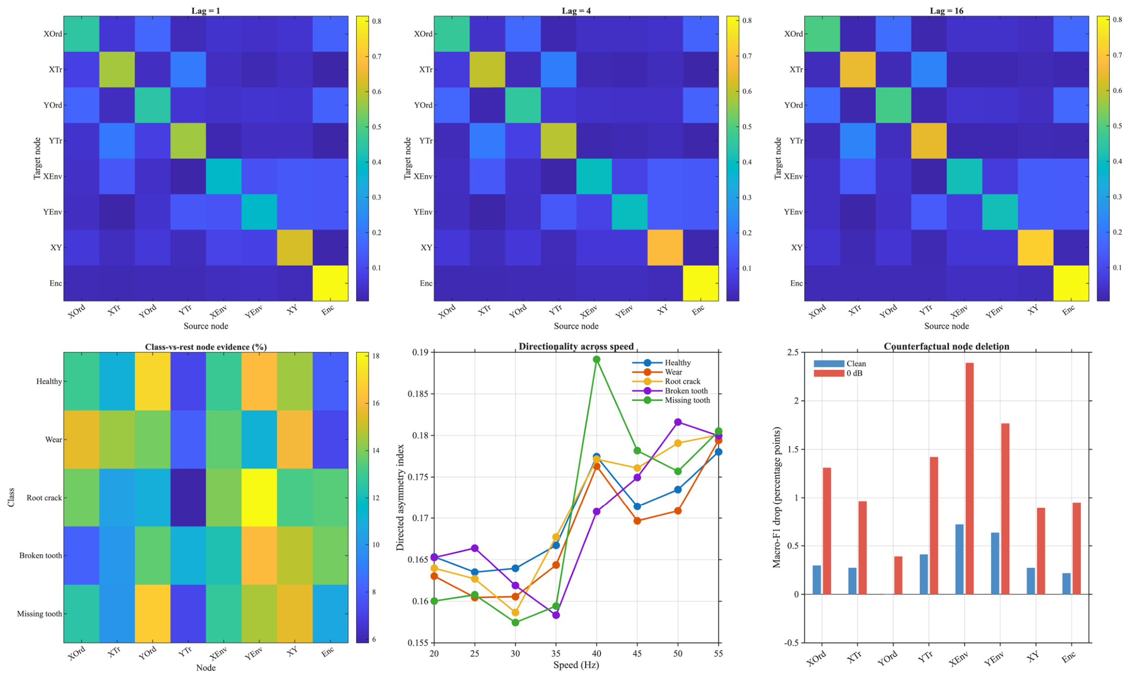
Figure 11, summarizes lag-specific adjacency, node sensitivity, and speed-dependent directionality. On clean files, macro-F1 was 99.66% for the graph branch, 99.64% for the local branch, and 99.63% after fusion. At 0 dB, the corresponding values were 96.27%, 96.48%, and 96.57%. Fusion therefore added only 0.09–0.30 percentage points under perturbation and was not the best branch for clean data. Its value is conditional: local peaks and graph relations can fail on different noisy samples, and posterior averaging reduces the chance that either failure controls the decision. This is a model-level observation and not a validated physical explanation.

Figure 11. Multi-lag directed graphs, node evidence, speed-dependent directionality, and counterfactual node occlusion.

Counterfactual deletion identified Y-envelope as the most influential node at 0 dB; setting it to zero reduced macro-F1 by 2.39 percentage points. Deleting the Y-order, XY-interaction, X-envelope, and encoder-speed nodes reduced macro-F1 by 1.77, 1.42, 1.31, and 0.95 points, respectively. Y-envelope particularly affected healthy and root-crack recall, whereas the XY-interaction was more influential for broken- and missing-tooth recall. These changes describe sensitivity to the constructed feature nodes; they do not verify a physical transfer path or fault location.

$$\Delta F{1}_v=F1\left(\mathbf{H}\right)-F1\left(\mathit{H}\odot (1-{\mathit{e}}_v)\right),v\in \{1,\dots ,8\}$$

(22)

Across all three lags, Y-transient → X-transient and X-transient → Y-transient were among the strongest connections, with mean weights near 0.21–0.23. Links between the X- and Y-order nodes were about 0.17–0.18, and encoder-speed → X/Y-order links were about 0.16–0.17. Simultaneous evidence in both directions is not contradictory, as within different phases and windows, either channel can carry predictive information about the other. Directional flux retains the difference between A and its transpose without asserting a unique one-way mechanical chain.

The direction-asymmetry index was generally near 0.16 at 20–30 Hz and rose to about 0.17–0.18 for many conditions at 40–55 Hz, although the trend was not strictly monotonic. Shorter impact intervals and changing transfer-path phase at higher speed may contribute to the observed variation, while installation differences explain local crossings. No single average adjacency should therefore be treated as representative of all speeds. Together, lagged edges, node deletion, and branch posteriors form a structured evidence report: a reported source-to-target association is identified, the corresponding feature node is removed to test whether held-out performance changes, and the branch posterior indicates whether the decision depended on local or propagated information.

3.8. Held-Out Installation and Speed Validation

The new tests probe condition shifts that the original balanced five-fold split could not isolate. Table 9 reports mean accuracy over two installation directions and four disjoint held-out speed pairs. The 40-file test set in each installation direction and 20-file test set in each speed pair are the independent recording units; window scores are retained to show within-file classification behavior.

Table 9. Held-out-condition accuracy (%, mean across two installation directions or four speed pairs). All comparators use the same training-file noise curriculum. The graph reference is a common-input implementation, not the published ESC-DGCN code.

Model/Variant	Installation Clean Window	Installation 0 dB Window	Installation Clean File	Speed Clean Window	Speed 0 dB Window
MLP + matched curriculum	69.71	67.11	70.00	97.09	92.62
Dual MLP + matched curriculum	70.00	67.19	72.50	97.25	92.60
Graph reference + matched curriculum	70.12	67.56	68.75	95.94	90.90
PG-MTCDGNet	71.39	68.12	72.50	96.64	91.33
Without direction	71.19	68.16	71.25	96.46	91.35
Without physical prior	70.61	67.71	70.00	96.56	91.46
Single lag	71.35	68.34	72.50	96.70	91.46
Without graph branch	70.21	67.52	71.25	96.97	92.38
Without local branch	72.17	68.28	70.00	96.31	90.84

Under the installation holdout, PG-MTCDGNet reached 71.39% clean-window accuracy, 1.68 percentage points above the matched MLP and 1.27 points above the controlled graph reference. Its 72.50% file-level accuracy equaled the dual-MLP control. The graph-only ablation reached 72.17% clean-window accuracy, above the full model’s 71.39%; at 0 dB, removing the direction or using one lag also slightly exceeded the full model. Across held-out speed pairs, PG-MTCDGNet averaged 96.64% on clean windows versus 97.09% for the MLP and 97.25% for the dual MLP. These results show a modest installation-specific gain in window accuracy, with no comprehensive superiority over the baselines or ablations. With only two installation directions and four speed groups from one rig, the differences are descriptive.

3.9. Performance of the Depth-Reduced Variant

PG-MTCDGNet-Lite achieved 88.13% four-condition file-level accuracy, exceeding the strong matched MLP’s 86.25% by 1.88 percentage points (Table 10). Its file-level macro-F1 was 88.04%, compared with 84.17% for the MLP. Clean file accuracy was 88.75% versus 86.25%. Secondary four-condition window accuracy was 79.50% versus 78.61%. These summaries include every installation direction, speed pair, and test condition rather than selecting a favorable subset.

Table 10. File-level accuracy (%) of the simplified model, retained controls, and matched Lite variants. Installation and speed-shift families have received equal weight; overall also weights the four conditions equally. All values are exploratory point estimates.

Model or Variant	Clean	−6 dB	0 dB	6 dB	Overall
PG-MTCDGNet-Lite	88.75	89.38	87.50	86.875	88.125
Matched MLP	86.25	84.38	86.25	88.13	86.25
Dual-MLP control	83.75	83.75	85.00	83.75	84.06
Controlled dynamic graph	85.63	82.50	83.75	84.38	84.06
Lite: Undirected graph	88.13	88.75	87.50	87.50	87.97
Lite: Single lag	87.50	88.75	87.50	86.88	87.66
Lite: Edge prior restored	88.75	88.75	87.50	86.88	87.97
Lite: Graph removed	88.13	88.75	88.13	87.50	88.13
Lite: Identity adjacency	88.13	88.75	88.13	87.50	88.13
Lite: Physical tokens removed	40.63	37.50	42.50	43.75	41.09

The component results qualify this gain. Undirected adjacency, one lag, and restoring the edge prior produced overall accuracies of 87.97%, 87.66%, and 87.97%, respectively. Removing the 96 physical tokens reduced accuracy to 41.09%. However, removing graph propagation or replacing adjacency with the identity matrix tied the full Lite model at 88.13%; their macro-F1 was slightly higher at 88.10%. The directed graph explicitly represents lag-dependent associations among physical nodes, providing a framework for investigating cross-node information under changing operating conditions. Although the present ablations do not establish an additional accuracy gain from graph propagation, this representation offers a testable research direction: determining when such associations provide diagnostic information beyond local descriptors.

4. Discussion

4.1. Boundaries of the Accuracy and Robustness Claims

The original matched-curriculum controls attribute most feature-noise robustness to training rather than graph structure. The new depth-reduced variant improves the designated four-condition file summary over the retained MLP, but an equally shallow non-graph control ties its accuracy. The evidence therefore favors a compact classifier with physically organized descriptors while leaving the additional predictive value of graph propagation unresolved.

Installation transfer remains harder than the balanced five-fold task. The 99.61% five-fold accuracy and Table 9 describe the dual-branch architecture; conversely, Table 10 describes Lite under the condition holdouts. Lite’s 1.86-percentage-point advantage over the MLP is an exploratory point estimate, without established statistical significance or specimen-independent validation.

The graph representation preserves the ordered lagged associations and directional readouts that can be examined alongside local descriptors. This makes it a candidate for studying how cross-node information varies with operating conditions. The equal overall accuracy of the shallow non-graph control indicates that the graph’s incremental predictive value remains unresolved on this dataset. Further research should test whether these associations offer additional diagnostic value on independent recordings and whether they agree with expert assessments or controlled physical measurements.

Performance near 100% makes leakage control especially important. Randomly dividing adjacent windows from one MAT file would allow training and test sets to share background noise, installation transfer functions, and slow speed trajectories. Grouping complete raw files prevents that form of segment leakage. However, it does not provide specimen-level independence: files from different folds may still originate from the same physical gear and rig. Recent leakage-aware evaluation work shows why component-wise separation matters when multiple independent components per class are available [49]. Because the WT benchmark lacks that diversity, the present result should be read as internal record-level validation rather than evidence of unseen-component generalization.

4.2. Model-Reported Structured Evidence

The graph repeatedly linked the X/Y-transient nodes, the X/Y-angle-domain nodes, and encoder micro-speed to vibration nodes across all three lags. The general increase in direction asymmetry with speed is consistent with changes in the observed cross-channel timing features as impact intervals shorten. Counterfactual deletion localizes the model’s reported sensitivity; Y-envelope, Y-order, and XY-interaction nodes were the most influential at 0 dB. These are associations in the learned representation, not validated mechanical paths.

The importance of Y-envelope is rig-specific and consistent with the feature construction. Envelope demodulation separates a carrier-related component from an amplitude-modulation descriptor, and the model assigned greater deletion sensitivity to the Y-direction feature at low SNRs on this rig. This association does not establish that the Y-direction contains the physical fault source or justify a universal sensor preference. Changing sensor orientation or support stiffness would be a useful external test of whether the counterfactual ranking persists.

Encoder micro-speed was not the leading deletion feature but contributed consistently to incoming edges of the angle-domain vibration nodes. Its role is closer to an operating reference than a direct fault marker. Within-window speed variation helps separate order drift caused by rotational fluctuation from modulation caused by damage. Speed and installation identifiers are never supplied to the class head, reducing the risk that the model learns a condition-to-label shortcut.

For a maintenance operator, the model can report a predicted state, supporting nodes, parent edges, lag scales, and the performance change after deletion. These items form a structured evidence package rather than a verified explanation. A root-crack decision, for example, can be accompanied by the contributions of Y-envelope and the X/Y-order nodes, encoder-speed modulation edges, and the three lag weights. Whether those signals correspond to the actual fault location should be checked by an expert or a physical experiment before they are used to trigger maintenance.

4.3. Limitations and Generalizability

The main limitation is external validity. The WT benchmark spans two installations and eight speeds, but all recordings share the same gear geometry, housing, acquisition chain, and a limited set of physical fault specimens. The model may therefore exploit order relationships or specimen signatures specific to this rig. A convincing external study should add at least one gearbox with different tooth counts or sensor placement and multiple independent components per health class, and should pre-specify the available speed range, condition composition, and missing-condition cases. The lags, k, and prior-floor value should remain fixed during that evaluation; a separately nested sensitivity analysis should then test whether conclusions persist across nearby settings. In addition, all 80 recordings informed repeated architecture development. The Lite comparison should be confirmed once on new raw recordings after freezing the architecture and training-fold selection rule.

Noise was added independently in a standardized node-feature space. This design isolates the classifier’s response to feature perturbation, but it does not represent colored background vibration, periodic electromagnetic interference, clipping, missing encoder pulses, sampling loss, or a loose sensor. A stricter test should perturb the raw X/Y/encoder waveforms, repeat phase synchronization and node construction, and report preprocessing failure rates in addition to classification accuracy. Such a test requires sensor- and acquisition-specific disturbance models and is therefore identified as necessary external validation rather than claimed by the present feature-noise results.

Past-to-future correlation excludes some reverse-time associations but cannot remove confounding by common speed excitation, housing resonance, or an unmeasured load. The physical prior, sparse incoming edges, and node-deletion tests organize the reported evidence; they do not convert the adjacency into a physical transmission law. Controlled impact tests, channel masking, load interventions, and structural equation modeling would be required to verify a physical interpretation.

The current task is closed-set recognition of five states. Unseen or compound faults and continuous degradation were not evaluated. A model with near-perfect AUC can still assign a known overconfident label to an unknown state. Future work should include leave-one-fault-out evaluation, independent temperature or conformal calibration, and human annotation of whether the reported evidence points to the correct physical location. The ESC-DGCN comparator is also a common-input MATLAB implementation rather than a run of the authors’ original code, so conclusions apply to the controlled reference implementation used here.

4.4. Computational Complexity and Deployment

Graph induction uses V = 8 nodes, L = 3 lags, and an angle-domain sequence of length T. Direct evaluation of every ordered pair costs O(LV²T). After top-k selection, one-hop propagation costs O(Vkd), and two-hop propagation is obtained by another sparse multiplication. Because V and k are small constants, phase synchronization, node construction, and the two compact classification heads dominate runtime rather than the adjacency itself. End-to-end latency on a target deployment device was not measured, so real-time performance remains unverified.

$$C_{graph}=O\left(L{V}^{2}T\right)+2O\left(Vkd\right),L=3,V=8,k=3$$

(23)

Offline operation estimates normalization statistics, trains both branches, and fixes the physical prior. Online operation constructs eight nodes for a new window, updates three sparse adjacencies, and produces the fused posterior. A deployment benchmark should report median and 95th-percentile end-to-end latency after warm-up, with batch size one, and should include acquisition, phase synchronization, feature construction, graph induction, and classification on the target controller. Edge weights and branch posteriors can be reported for every window, whereas the eight additional node-deletion passes can run asynchronously after an alarm. Direction-asymmetry summaries are better suited to periodic maintenance review.

A deployed system also requires an abstention rule. A low maximum posterior, disagreement between the two branches, or a key-edge pattern outside the training distribution should produce an uncertain state rather than a forced five-class label. Branch disagreement can be measured by Jensen–Shannon divergence and combined with maximum posterior and deletion stability. This rule was not included in the closed-set score and should be validated under unknown faults before deployment.

$$D_{JS}({\mathbf{p}}_c,{\mathbf{p}}_l)={\displaystyle \frac{1}{2}}{D}_{KL}({\mathbf{p}}_c\Vert \mathbf{m})+{\displaystyle \frac{1}{2}}{D}_{KL}({\mathbf{p}}_l\Vert \mathbf{m}),\mathbf{m}={\displaystyle \frac{{\mathit{p}}_c+{\mathit{p}}_l}{2}}$$

(24)

5. Conclusions

PG-MTCDGNet organizes phase-synchronous X/Y-vibration, transient residuals, envelopes, cross-channel coupling, and encoder micro-speeds into an eight-node graph. Directed top-k adjacencies from lags of one, four, and 16 samples are combined with graph shrinkage, unsmoothed local evidence, posterior fusion, and a noise-consistency curriculum. Under balanced, raw-file-isolated five-fold validation of 80 recordings and 5120 windows, the model achieved 99.61% ± 0.33% accuracy and 99.63% ± 0.31% macro-F1. These scores establish performance for the supplied implementation and protocol; they do not establish superiority over published ESC-DGCN or a unique graph contribution.

The controls place these numbers in context. Removing the consistency curriculum reduced 0 dB macro-F1 to 82.58%, whereas supplying the same curriculum to deep MLP and the ESC-DGCN-style controlled reference brought all three deep models to an average accuracy near 95.4% across six SNRs. Noise robustness is therefore primarily a training effect. Multi-scale directionality and the physical prior did not consistently increase closed-set accuracy on this dataset. Their supported contribution is limited to organizing lagged edges, graph and local posteriors, and node-occlusion responses as structured outputs; none of these outputs has been expert-validated as a physical explanation.

The present evidence supports PG-MTCDGNet as a reproducible structured-evidence framework for a single multi-installation, multi-speed planetary-gearbox benchmark. It does not establish intervention effects, expert-confirmed explanations, physical verification of edge meanings, published-baseline superiority, specimen-independent or cross-rig generalization, raw-sensor robustness, open-set reliability, or real-time latency on a target controller. External tests with multiple physical specimens, independent rig or gear geometry, raw-waveform disturbances, official reference implementations, and human or physical validation of evidence localization are required before stronger diagnostic claims can be made.

The depth-reduced PG-MTCDGNet-Lite reached 88.125% four-condition file accuracy and 88.044% macro-F1, compared with 86.250% and 84.171% for the retained MLP. A shallow non-graph ablation tied its accuracy, preventing a claim that every graph component is required. This exploratory result supports model simplification and motivates a frozen comparison on new recordings; it does not replace independent validation.

References

- Liu, D.; Cui, L.; Cheng, W. A review on deep learning in planetary gearbox health state recognition: Methods, applications, and dataset publication. Meas. Sci. Technol. 2024, 35, 012002. [Google Scholar] [CrossRef] [Scilit]
- Liu, D.; Cui, L.; Wang, H. Rotating machinery fault diagnosis under time-varying speeds: A review. IEEE Sens. J. 2023, 23, 29969–29990. [Google Scholar] [CrossRef] [Scilit]
- Zhu, Z.; Lei, Y.; Qi, G.; Chai, Y.; Mazur, N.; An, Y.; Huang, X. A review of the application of deep learning in intelligent fault diagnosis of rotating machinery. Measurement 2023, 206, 112346. [Google Scholar] [CrossRef] [Scilit]
- Li, T.; Zhou, Z.; Li, S.; Sun, C.; Yan, R.; Chen, X. The emerging graph neural networks for intelligent fault diagnostics and prognostics: A guideline and a benchmark study. Mech. Syst. Signal Process. 2022, 168, 108653. [Google Scholar] [CrossRef] [Scilit]
- Yang, C.; Liu, J.; Zhou, K.; Jiang, X.; Zeng, X. An improved multi-channel graph convolutional network and its applications for rotating machinery diagnosis. Measurement 2022, 190, 110720. [Google Scholar] [CrossRef] [Scilit]
- Cao, S.; Li, H.; Zhang, K.; Yang, C.; Xiang, W.; Sun, F. A novel spiking graph attention network for intelligent fault diagnosis of planetary gearboxes. IEEE Sens. J. 2023, 23, 13140–13154. [Google Scholar] [CrossRef] [Scilit]
- Chen, Z.; Ji, J.; Yu, W.; Ni, Q.; Lu, G.; Chang, X. A multi-scale graph convolutional network with contrastive-learning enhanced self-attention pooling for intelligent fault diagnosis of gearbox. Measurement 2024, 230, 114497. [Google Scholar] [CrossRef] [Scilit]
- Wang, L.; Xie, F.; Zhang, X.; Jiang, L.; Huang, B. Spatial-temporal graph feature learning driven by time-frequency similarity assessment for robust fault diagnosis of rotating machinery. Adv. Eng. Inform. 2024, 62, 102711. [Google Scholar] [CrossRef] [Scilit]
- Li, C.; Mo, L.; Kwoh, C.K.; Li, X.; Chen, Z.; Wu, M.; Yan, R. Noise-robust multi-view graph neural network for fault diagnosis of rotating machinery. Mech. Syst. Signal Process. 2025, 224, 112025. [Google Scholar] [CrossRef] [Scilit]
- Wang, C.; Wang, Y.; Wang, Y.; Li, X.; Chen, Z. Richly connected spatial-temporal graph neural network for rotating machinery fault diagnosis with multi-sensor information fusion. Mech. Syst. Signal Process. 2025, 225, 112230. [Google Scholar] [CrossRef] [Scilit]
- Li, X.; Ran, G.; Xiao, S.; Su, K.; Li, Q.; Wang, T.; Qin, Z.; Chu, F.L. A fault diagnosis method for bearings based on multiscale graph convolutional network under non-stationary speed conditions. Mech. Mach. Theory 2025, 217, 106267. [Google Scholar] [CrossRef] [Scilit]
- Liu, H.; Sun, Y.; Wang, X.; Wang, H. Degree bias mitigation and noise robustness for rotating machinery fault detection. Mech. Syst. Signal Process. 2025, 239, 113338. [Google Scholar] [CrossRef] [Scilit]
- Li, X.; Wang, Y.; Xing, J.; Wang, Y. Causal graph inference with adaptive dynamic structure learning for mechanism-oriented fault diagnosis in dynamic industrial systems. Reliab. Eng. Syst. Saf. 2026, 266, 111865. [Google Scholar] [CrossRef] [Scilit]
- Wang, C.; Xu, M.; Li, Y.; Zhang, Q.; Zhang, D.; Liu, B. A novel two-stage fault diagnosis method with frequency-aware graph contrastive learning and multi-scale recursive graph networks for rotating machinery. Adv. Eng. Inform. 2026, 70, 104196. [Google Scholar] [CrossRef] [Scilit]
- Li, X.; Wang, C.; Wang, H.; Wang, T.; Chu, F. Spatiotemporal graph neural diagnostics for rotating machinery: A single-sensor multidimensional fusion framework. Struct. Health Monit. 2026, 14759217251414064. [Google Scholar] [CrossRef] [Scilit]
- Li, X.; Yang, T.; Lin, B.; Jiang, S.; Han, Q.; Gong, Y.; Wang, X. Pioneering graph-enhanced diagnostics for bearings with interpretability. Eng. Appl. Artif. Intell. 2026, 180, 115173. [Google Scholar] [CrossRef] [Scilit]
- Li, Y.; Zhang, L.; Liang, P.; Wang, X.; Wang, B.; Xu, L. Semi-supervised meta-path space extended graph convolution network for intelligent fault diagnosis of rotating machinery under time-varying speeds. Reliab. Eng. Syst. Saf. 2024, 251, 110363. [Google Scholar] [CrossRef] [Scilit]
- Xiao, X.; Li, C.; He, H.; Huang, J.; Yu, T. Rotating machinery fault diagnosis method based on multi-level fusion framework of multi-sensor information. Inf. Fusion 2024, 113, 102621. [Google Scholar] [CrossRef] [Scilit]
- Deng, Q.; Chen, Z.; Zhu, W.; Li, Z.; Yuan, Y.; Wang, Y. Adaptive fusion graph convolutional network based interpretable fault diagnosis method for HVAC systems enhanced by unlabeled data. Energy Build. 2024, 324, 114901. [Google Scholar] [CrossRef] [Scilit]
- Shan, D.; Cheng, C.; Li, L.; Peng, Z.; He, Q. Semisupervised fault diagnosis of gearbox using weighted graph-based label propagation and virtual adversarial training. IEEE Trans. Instrum. Meas. 2023, 72, 3503411. [Google Scholar] [CrossRef] [Scilit]
- Pu, Z.; Cabrera, D.; Bai, Y.; Li, C. A one-class generative adversarial detection framework for multifunctional fault diagnoses. IEEE Trans. Ind. Electron. 2022, 69, 8411–8419. [Google Scholar] [CrossRef] [Scilit]
- Zhou, K.; Diehl, E.; Tang, J. Deep convolutional generative adversarial network with semi-supervised learning enabled physics elucidation for extended gear fault diagnosis under data limitations. Mech. Syst. Signal Process. 2023, 185, 109772. [Google Scholar] [CrossRef] [Scilit]
- Liang, K.; Zhao, M.; Lin, J.; Jiao, J.; Ding, C. Toothwise health monitoring of planetary gearbox under time-varying speed condition based on rotating encoder signal. IEEE Trans. Ind. Electron. 2022, 69, 6267–6277. [Google Scholar] [CrossRef] [Scilit]
- Li, M.; Wang, T.; Kong, Y.; Chu, F. Synchro-reassigning transform for instantaneous frequency estimation and signal reconstruction. IEEE Trans. Ind. Electron. 2022, 69, 7263–7274. [Google Scholar] [CrossRef] [Scilit]
- Zhang, D.; Feng, Z. Proportion-extracting chirplet transform for nonstationary signal analysis of rotating machinery. IEEE Trans. Ind. Inform. 2023, 19, 2674–2683. [Google Scholar] [CrossRef] [Scilit]
- Zhang, K.; Li, H.; Cao, S.; Yang, C.; Sun, F.; Wang, Z. Motor current signal analysis using hypergraph neural networks for fault diagnosis of electromechanical system. Measurement 2022, 201, 111697. [Google Scholar] [CrossRef] [Scilit]
- Wang, X.; Si, S.; Li, Y. Variational embedding multiscale diversity entropy for fault diagnosis of large-scale machinery. IEEE Trans. Ind. Electron. 2022, 69, 3109–3119. [Google Scholar] [CrossRef] [Scilit]
- Zhang, Z.; Yang, Q.; Zi, Y.; Wu, Z. Discriminative sparse autoencoder for gearbox fault diagnosis toward complex vibration signals. IEEE Trans. Instrum. Meas. 2022, 71, 3522611. [Google Scholar] [CrossRef] [Scilit]
- Shao, H.; Xia, M.; Wan, J.; de Silva, C.W. Modified stacked autoencoder using adaptive Morlet wavelet for intelligent fault diagnosis of rotating machinery. IEEE/ASME Trans. Mechatron. 2022, 27, 24–33. [Google Scholar] [CrossRef] [Scilit]
- Wang, H.; Liu, Z.; Peng, D.; Cheng, Z. Attention-guided joint learning CNN with noise robustness for bearing fault diagnosis and vibration signal denoising. ISA Trans. 2022, 128, 470–484. [Google Scholar] [CrossRef] [Scilit]
- Tang, J.; Zheng, G.; Wei, C.; Huang, W.; Ding, X. Signal-transformer: A robust and interpretable method for rotating machinery intelligent fault diagnosis under variable operating conditions. IEEE Trans. Instrum. Meas. 2022, 71, 3511911. [Google Scholar] [CrossRef] [Scilit]
- Kim, Y.; Na, K.; Youn, B.D. A health-adaptive time-scale representation embedded convolutional neural network for gearbox fault diagnostics. Mech. Syst. Signal Process. 2022, 167, 108575. [Google Scholar] [CrossRef] [Scilit]
- Jiang, L.; Li, S.; Li, X.; Lei, J.; Yang, D. Fault diagnosis of a planetary gearbox based on a local bi-spectrum and a convolutional neural network. Meas. Sci. Technol. 2022, 33, 045008. [Google Scholar] [CrossRef] [Scilit]
- Huang, D.; Zhang, W.A.; Guo, F.; Liu, W.; Shi, X. Wavelet packet decomposition-based multiscale CNN for fault diagnosis of wind turbine gearbox. IEEE Trans. Cybern. 2023, 53, 443–453. [Google Scholar] [CrossRef] [Scilit]
- Han, S.; Shao, H.; Cheng, J.; Yang, X.; Cai, B. Convformer-NSE: A novel end-to-end gearbox fault diagnosis framework under heavy noise using joint global and local information. IEEE/ASME Trans. Mechatron. 2023, 28, 340–349. [Google Scholar] [CrossRef] [Scilit]
- Sun, W.; Wang, H.; Xu, J.; Yang, Y.; Yan, R. Effective convolutional transformer for highly accurate planetary gearbox fault diagnosis. IEEE Open J. Instrum. Meas. 2022, 1, 3500209. [Google Scholar] [CrossRef] [Scilit]
- Zhang, Y.; Ren, Z.; Feng, K.; Yu, K.; Ma, H.; Liu, Z. Transformer-enabled cross-domain diagnostics for complex rotating machinery with multiple sensors. IEEE/ASME Trans. Mechatron. 2023, 28, 2293–2304. [Google Scholar] [CrossRef] [Scilit]
- Weng, C.; Lu, B.; Gu, Q.; Zhao, X. A novel multisensor fusion transformer and its application into rotating machinery fault diagnosis. IEEE Trans. Instrum. Meas. 2023, 72, 3507512. [Google Scholar] [CrossRef] [Scilit]
- Zhang, Y.; Feng, K.; Ma, H.; Yu, K.; Ren, Z.; Liu, Z. MMFNet: Multisensor data and multiscale feature fusion model for intelligent cross-domain machinery fault diagnosis. IEEE Trans. Instrum. Meas. 2022, 71, 3526311. [Google Scholar] [CrossRef] [Scilit]
- Xu, Z.; Bashir, M.; Zhang, W.; Yang, Y.; Wang, X.; Li, C. An intelligent fault diagnosis for machine maintenance using weighted soft-voting rule based multi-attention module with multi-scale information fusion. Inf. Fusion 2022, 86–87, 17–29. [Google Scholar] [CrossRef] [Scilit]
- Xie, T.; Huang, X.; Choi, S.K. Intelligent mechanical fault diagnosis using multisensor fusion and convolution neural network. IEEE Trans. Ind. Inform. 2022, 18, 3213–3223. [Google Scholar] [CrossRef] [Scilit]
- Zhang, Y.; Ji, J.C.; Ren, Z.; Ni, Q.; Wen, B. Multi-sensor open-set cross-domain intelligent diagnostics for rotating machinery under variable operating conditions. Mech. Syst. Signal Process. 2023, 191, 110172. [Google Scholar] [CrossRef] [Scilit]
- Zhang, Y.; Ren, Z.; Feng, K.; Yu, K.; Beer, M.; Liu, Z. Universal source-free domain adaptation method for cross-domain fault diagnosis of machines. Mech. Syst. Signal Process. 2023, 191, 110159. [Google Scholar] [CrossRef] [Scilit]
- Chen, P.; Zhao, R.; He, T.; Wei, K.; Yuan, J. A novel bearing fault diagnosis method based on joint attention adversarial domain adaptation. Reliab. Eng. Syst. Saf. 2023, 237, 109345. [Google Scholar] [CrossRef] [Scilit]
- Siddique, M.F.; Zaman, W.; Khalid, M.; Hamdan, B.; Kim, J.M. A multistage transfer learning framework for intelligent fault diagnosis of rotating machinery under variable operating conditions. Sci. Rep. 2026, 16, 18489. [Google Scholar] [CrossRef] [Scilit]
- Siddique, M.F.; Bourezg, A.; Wisal, M.; Ali, S.; Umar, M.; Saleem, F.; Janjua, M.M. Bearing fault diagnosis: Class-conditional deep domain adaptation for generalization across machines. In Proceedings of the 2026 International Conference on Robotics and Automation in Industry (ICRAI), Islamabad, Pakistan, 4–5 May 2026; pp. 1–7. [Google Scholar] [CrossRef] [Scilit]
- Matania, O.; Bechhoefer, E.; Blunt, D.; Wang, W.; Bortman, J. Anomaly detection and remaining useful life estimation for the Health and Usage Monitoring Systems 2023 Data Challenge. Sensors 2024, 24, 4258. [Google Scholar] [CrossRef] [Scilit]
- Huang, L.T.; Chang, J.Y. Vibration characterization and fault diagnosis of a planetary gearbox with a wireless embedded sensor. Appl. Sci. 2023, 13, 729. [Google Scholar] [CrossRef] [Scilit]
- Vieira, J.P.; Bauler, V.A.; Rosa, R.K.; Silva, D. Towards a more realistic evaluation of machine learning models for bearing fault diagnosis. Mech. Syst. Signal Process. 2026, 258, 114640. [Google Scholar] [CrossRef] [Scilit]
Disclaimer/Publisher’s Note: The statements, opinions and data contained in all publications are solely those of the individual author(s) and contributor(s) and not of MDPI and/or the editor(s). MDPI and/or the editor(s) disclaim responsibility for any injury to people or property resulting from any ideas, methods, instructions or products referred to in the content. |
© 2026 by the authors. Licensee MDPI, Basel, Switzerland. This article is an open access article distributed under the terms and conditions of the Creative Commons Attribution (CC BY) license.