


Abstract
Elevated string-rail systems, in which unmanned electric vehicles run on steel wheels along a prestressed rail carried on slender supports, have been proposed as a way of moving containers between a quay and an inland terminal without using the road network. Their developers claim gains in ship handling speed, terminal land use and emissions at the same time, but none of these claims has been tested against measured port performance. This study assesses such a link at eight European container ports handling between 0.4 and 14.2 million TEU. The assessment combines two distinct components: a discrete-event simulation of the quay interface, calibrated against the Container Port Performance Index to within 1.5% of reported ship time at berth, and separate analytical calculations of required yard area, emissions and cost. The simulation covers the crane and horizontal-transport interface only; stacking, retrieval, reshuffling and yard-crane operations are outside its boundary. Internal model behaviour is benchmarked against independently published terminal operating figures, and the logic, inputs and scenario behaviour of the model were assessed by four specialists in container terminal operations. Because no published source gives the energy use of the vehicle, it is derived from physics, specifically from rolling and aerodynamic resistance, as 0.482 kWh per TEU-km. On an analytical capacity calculation, removing half of the road-borne inland volume would reduce required stacking area by 7.7 to 31.6%, equivalent to between 4.2 and 108.6 hectares of terminal area under a stated proportionality assumption, and a conditional comparison of emission factors gives a reduction of 60 to 97% on the diverted traffic alone. Avoided road haulage gives a positive annual balance at seven of the eight ports, with simple payback of 3.5 to 5 years at the five largest diverted flows. The benefit depends on how much of a port’s traffic actually leaves by road: gateway ports with heavy road use gain most, while a transhipment hub such as Piraeus gains least despite its size. Ship handling improves by at most 3.8%, well below the 5 to 10% claimed, and the improvement comes from avoiding the drive across the yard rather than from a faster crane cycle. Measured against the price of carbon, the investment is poor value, but measured against the cost of road haulage, it is not, which suggests such links should be planned as land and traffic infrastructure rather than as an emissions measure.
1. Introduction
Container terminals are squeezed from three directions at once. Ships have grown faster than the quays that serve them, land near the sea has run out in most European ports, and the trucks that carry containers inland remain the dirtiest and least predictable part of the journey. Anything done about one of these tends to make another worse. A bigger stacking yard needs land the port does not have. More cranes need more vehicles driving between quay and yard. Clearing the yard faster pushes the queue out to the gate.
Elevated string-rail transport has been put forward as a solution to these issues. The idea is simple enough: a prestressed steel rail carried on widely spaced supports, above the ground and above whatever is already there, with small unmanned electric vehicles running along it on steel wheels [1,2]. Because the structure only touches the ground at its supports, it occupies almost no land. Because the wheel is steel on steel, rolling resistance is low. Because the vehicles are automated, they can run close together. Suppliers of the technology claim that a line installed inside the crane portal would speed up ship handling by 5 to 10%, that it would free terminal land, and that it would cut emissions.
The claims are plausible. None of them has been checked. The technology has been built at two demonstration sites but never at a working container terminal, so no operating data exist, and the published figures come from the company that makes it.
1.1. Background Work
How containers move between quay and yard has been studied for decades, and the problem is well understood [3,4]. A quay crane cannot finish a lift until a vehicle is underneath it, so the size of the vehicle fleet, the way it is dispatched and the distance it must travel all feed straight through into how fast a ship is worked [5]. The alternatives have been catalogued and compared: tractor-trailer sets, straddle carriers, automated guided vehicles (AGV), and automated lifting vehicles [6,7]. Work on yard layout shows how strongly block geometry and stacking height interact with the vehicles that serve them [8,9,10]. Simulation has been the usual tool throughout, and reviews of terminal simulation note a recurring weakness: models are often built on synthetic or private data and cannot be checked by anyone else [11].
What the vehicle comparisons agree on is that no single choice is best everywhere. Straddle carriers lift containers themselves and so decouple the crane from the yard, at the cost of higher maintenance and a taller stack. Tractor-trailer sets are cheap and flexible but tie the crane to the arrival of a driver. Automated vehicles remove the driver and the variability that comes with one, but they need a controlled surface and a large fleet, since an automated vehicle that cannot lift its own load waits under the crane and waits again at the stack. Every one of these trade-offs is a trade-off about ground-level movement, and none of them removes the movement itself.
All of these vehicles have one thing in common. They travel on the ground, inside the terminal, and their cycle time grows as the terminal grows. To keep pace, the fleet has to grow faster than the traffic it serves [12]. A link that leaves the terminal altogether would not care about the shape of the yard, which is the main argument for building one.
There is a second reason the geometry matters, which the yard layout studies bring out clearly. Longer travel does not only cost time; it costs predictability. A vehicle crossing a busy terminal shares its route with other vehicles, crosses working lanes and queues at transfer points, so the spread of its journey times widens faster than the average does. Cranes are sized against the worst of that spread rather than the middle of it, which is why terminals carry more vehicles than a simple throughput calculation would suggest.
The gate is the second pressure point. Truck congestion at terminal gates has produced its own literature on appointment systems, arrival windows and chassis exchange [13,14,15], all of which manage the queue rather than remove it. A link that never crosses the gate removes it by design, though at considerable cost.
Where the containers go afterwards has been studied under several names. Port regionalisation describes how ports have extended themselves inland along rail and barge corridors [16]. Terminalisation describes terminals taking an active role further along the chain, acting either as a bottleneck or as a buffer [17]. The dry port concept describes the inland site that receives containers moved out of the port early [18], sometimes under the terminal operator’s own control as an extended gate [19], and its development depends on whether the initiative comes from the coast or from inland [20]. Whether moving containers inland early actually reduces emissions and cost is less settled than the concept’s popularity suggests; it depends heavily on how far the inland site is and how the containers get there [21,22,23]. The same threshold behaviour is familiar from intermodal transport more generally, where handling cost and distance together decide whether a fixed link beats a truck [24,25]. Standard treatments of port economics set all of this in its commercial context [26].
The pressure on land is severe and getting worse. Antwerp and Rotterdam each cover more ground than the cities they belong to, and further growth now means reclaiming land from the sea or moving somewhere else, both expensive. Ports hemmed in by terrain, of which Rijeka is a clear case, have no room at all. How ports with limited space have coped with ever-larger ships has been examined directly [27], as has the wider reshaping of shipping networks that put them under pressure in the first place [28,29]. Where a port handles more than containers, every hectare given to stacking is a hectare taken from something else.
On emissions, reviews of port energy use and terminal carbon accounting agree on where the emissions are [30,31,32]. Road haulage inland is usually the largest single source for a gateway port, and it is the hardest for a port to do anything about, since it happens outside the fence [33]. A wide range of measures has been proposed, from cleaner ships [34] to near-zero-energy ports [35], smarter energy management [36] and terminal-level carbon strategies [37]. Studies of individual equipment changes, such as electrifying rubber-tyred gantries or replacing terminal vehicles, come closest to what is attempted here in method [38,39], though they change equipment inside the terminal rather than replacing the journey. Measurements from Valencia are directly relevant, since Valencia is one of the ports studied below [40].
Two habits in this literature are worth naming because this study avoids both. Electricity is usually given a single emission factor, which hides the fact that the same electric machine performs very differently in France and in Poland. And the thing being replaced is almost always a diesel truck, which is the easiest comparison to win; at a Rhine or Scheldt port the realistic alternative is a barge or an electric train, and those comparisons are rarely made.
Finally, string rail belongs to a family of ideas for getting freight off the road that have mostly failed to reach commercial scale. Underground freight networks were studied seriously in the Netherlands [41] and reviewed critically elsewhere, with capital cost and network effects rather than engineering identified as the obstacle [42]. Aerial ropeways have found niches in cities and in mining, and their engineering literature is useful about what maintaining a suspended system involves [43]. String rail differs from these in that the load is carried by a stiff prestressed rail rather than a flexible rope, so the vehicle rolls on steel rather than riding a cable. That is where its efficiency claim comes from, and it also means the structure costs more like an elevated railway than like a ropeway. What none of these proposals has settled is how much traffic a dedicated link needs before it beats the shared road network. That threshold is what this study estimates for the container port case.
Table 1 places this study against representative earlier work along the six dimensions that define its scope: how the system was modelled, which transport technology was examined, whether the model or the accounting was checked against measured data, and whether land use, emissions and economics were assessed. The pattern in the table is the gap. Terminal operations research models horizontal transport in detail and checks it against operational data, but confines itself to equipment that already exists and rarely costs or carbons its findings. The alternative-conveyance literature examines novel technologies but stops at feasibility, with no terminal model behind it. The hinterland and port-emission literature assesses emissions and sometimes cost, but treats the terminal as a point. No entry combines a calibrated quay-side model of a novel conveyance with land, emission and cost assessment at the same set of real ports.
Table 1.
Representative previous studies and the dimensions covered. DES = discrete-event simulation. Empirical basis records whether model behaviour or accounting was compared with measured data.
Three things are missing from the picture. Nobody has put an elevated conveyance system inside a container terminal model that has been checked against real performance data; the engineering literature describes the vehicle and the port literature ignores it. Port emission studies rarely test their proposed change against the mode it would genuinely displace at that particular port, and almost never against more than one. And the three benefits claimed for this kind of system have never been separated, so it is not known whether they come from the same cause or whether they simply appear on the same page of a brochure.
1.2. Aim of This Research
This study asks what an elevated string-rail link would actually do at a real European container port, using a model checked against independent performance measurements rather than supplier figures. Three questions follow. How much would it change ship handling speed? How much terminal land would it free? And against which alternative, at which national electricity mix, would it genuinely reduce emissions?
The study contributes in three ways: (i) It derives the vehicle’s energy use from physics, because no published figure exists. (ii) It calibrates a terminal simulation against the Container Port Performance Index, so the starting point is measured rather than assumed. (iii) It separates the three claimed benefits and shows that they do not come from the same cause, which changes how such a project should be judged.
Ports where the technology performs badly are kept in the sample deliberately. A transhipment hub and a small port with little traffic are included precisely because the link should struggle at both, and reporting where something fails is what separates an assessment from an advertisement.
2. Materials and Methods
The assessment combines two models. Ship time at berth depends on events at a single berth, so quay operations are simulated call by call, while yard area, emissions and cost depend on annual volumes and are calculated directly. Section 2.1 defines the system, the eight ports and the present operation against which everything is measured. Section 2.2 fixes the boundary of the simulation and states what is outside it. Section 2.3 gives the formal specification of the model, and Section 2.4 gives its inputs. Section 2.5, Section 2.6 and Section 2.7 deal with verification, calibration, the benchmarking of internal model behaviour against independent operating data, and an assessment of the model by specialists in terminal operations, since every result reported later is a difference from a calibrated starting point. Section 2.8 sets out the energy, land, emission and cost calculations.
2.1. The System, the Ports and the Alternative
The system modelled here runs an elevated line inside the ship-to-shore (STS) crane portal, takes containers directly from the spreader or from a small intermediate stack of one to three slots, crosses the terminal above it, and continues 5 to 30 km to an inland terminal. It therefore skips both the stacking yard and the truck gate. Figure 1 shows the arrangement alongside the ordinary route it replaces.
Figure 1.
The elevated link and the yard, gate and road haulage it replaces.
Other arrangements are conceivable. The line could serve only the terminal, moving containers from quay to stack; or a full two-level network could be built. Only the version modelled here produces all three claimed effects from one cause, since containers that leave the quay without touching the yard or the gate simultaneously shorten the crane’s reach, take trucks out of the port, and reduce the amount of yard needed. Replacing yard vehicles alone would leave land and emissions almost unchanged, and a full network adds so many untested connections that no measured starting point could anchor it. Table 2 lists what the manufacturer publishes. Every figure is treated here as a claim to be tested with a range around it, never as a measurement.
Table 2.
Published characteristics of the container vehicle and line.
Eight ports were selected to cover a wide spread of size, road dependence and electricity mix (Table 3). The spread matters more than the number. Throughput ranges over a factor of thirty-five, the share of containers transferred between ships ranges from a twentieth to four fifths, the share of inland traffic moving by road ranges from just under half to almost all of it, and the electricity used to run the line varies twelvefold between the cleanest and the dirtiest national supply in the sample. Any one of these could plausibly drive the result, and separating them is only possible if all four vary independently across the sample, which is why ports were chosen for contrast rather than for size. Each is paired with an inland terminal that already exists or is already planned, so the distances are real ones. Rijeka is included because it is the clearest case of a port with nowhere left to expand; the container depot at Škrljevo, ten kilometres inland, is being enlarged at present for exactly that reason. Piraeus is included because four-fifths of its containers are transferred between ships and never travel inland at all, so the link should do little for it.
Table 3.
The eight ports with the corresponding statistics.
Terminal areas, quay lengths, crane numbers and throughput were taken from port authority publications and terminal operator disclosures rather than from commercial databases, so that every figure can be traced. Where a port operates several deep-sea container terminals, the figures are the sum for those terminals only; barge berths, empty depots and feeder quays are excluded, since they are not on the path being modelled.
The comparison throughout is against how the port works today: containers cross the yard on terminal tractors, wait in the stack, leave through the gate and travel inland by truck. Deep-sea shipping, distribution beyond the inland terminal, the emissions of building the structure, and the rail and barge legs are all left out, the last of these held constant so they cannot distort the comparison.
2.2. Model Boundary and What Is Not Represented
Because the scope of the simulation determines how every later result should be read, it is stated explicitly before the model itself.
The discrete-event component is a quay-interface model. Its boundary begins at the quay crane hook and ends at the point where a container is handed to a horizontal transport unit, and that unit leaves the crane. Inside the boundary are vessel arrival, berth allocation, crane assignment, the crane work cycle, the availability of a horizontal transport unit under the crane, and the waiting that occurs when none is available.
Outside the boundary are stacking and retrieval, container reshuffling, the operation of yard cranes whether rubber-tyred, rail-mounted or reach stackers, internal traffic conflicts and routing, gate processing, and yard management strategy. These are represented only through their aggregate effect on the horizontal transport cycle time, which is treated as a random variable whose distribution is stated in Section 2.4. No claim is made that the model reproduces yard behaviour, and no result that depends on yard behaviour is derived from it.
This is a deliberate restriction rather than an omission. Representing stacking, reshuffling and yard-crane operations credibly requires terminal-specific layout, stacking policy and equipment data that is not publicly available for eight ports, and substituting assumed values would give the appearance of detail without its substance. The quantity the study needs from the simulation is the difference in crane waiting between two horizontal transport systems serving the same crane, and that difference is determined at the interface rather than in the stack.
The consequence is that the paper is not, and does not claim to be, an integrated simulation of terminal operations. It comprises four components with different methods and different epistemic status, set out in Table 4, and results should be attributed to the component that produced them.
Table 4.
Components of the assessment, their methods and their status.
2.3. Formal Specification of the Quay-Interface Model
Ship time at berth is a property of a single call, so a representative pair of berths reproduces it exactly without simulating the several thousand calls a large port receives each year. Time-based results therefore come from a discrete-event simulation of the quay, while yard area, emissions and cost are calculated annually from throughput. Figure 2 shows how the two fit together.
Figure 2.
How the model is designed.
The model is implemented in Python 3 with the SimPy discrete-event library [45]. Its formal structure is given below so that it can be reproduced independently.
Entities. Vessel calls, containers (aggregated as crane moves), quay cranes, and horizontal transport units.
Resources. A berth pool of capacity Nb; a crane set of capacity Nc per berthed vessel; and one of two horizontal transport resources, described below.
State variables. Number of vessels in service and in queue; per-crane remaining move count; number of idle transport units; cumulative crane waiting time; cumulative crane cycle time; and simulation clock.
Events. (i) vessel arrival; (ii) berth seizure; (iii) berthing manoeuvre completion; (iv) crane move request for a transport unit; (v) transport unit made available under the crane; (vi) crane cycle completion; (vii) transport unit released after its cycle; (viii) last crane finishes, unberthing begins; (ix) berth release.
Process logic. On arrival, a vessel requests a berth and queues first-come-first-served if none is free. On seizure, it incurs a fixed berthing time, then its total move count is divided as evenly as possible among the assigned cranes. Each crane then repeats the following until its share is exhausted: request a horizontal transport unit; wait, recording the waiting time separately, until one is available; execute one crane cycle of stochastic duration; release control. When all cranes finish, the vessel incurs a fixed unberthing time and releases the berth.
Horizontal transport, baseline. A pool of nt = λ Nc tractor units, where λ is the fleet ratio per crane. A unit becomes available to the crane immediately if the pool is non-empty; it is then occupied for a stochastic round-trip time representing travel to the stack, transfer and return, after which it rejoins the pool. Queue discipline is first-come-first-served across cranes. The round-trip distribution is the only channel through which yard conditions enter the model.
Horizontal transport, elevated link. A carrier is presented at the crane every h/nL seconds, where h is the published minimum headway, and nL is the number of lines. The supply process is modelled as a bounded store of capacity one per line: a carrier arriving when no container is ready is not held but passes empty, and the next carrier arrives one interval later. A crane requesting a carrier therefore waits a residual time uniformly distributed on [0, h/nL] in expectation. In the buffered variant, an intermediate stack of s slots is interposed: the crane deposits into the stack and is blocked only when the stack is full, while carriers remove from the stack at the headway interval. Blocking, empty running and the residual-wait mechanism are therefore all represented explicitly; what is not represented is a dispatching policy that would allocate carriers preferentially among competing cranes, because at the line capacities considered, the supply process is interval-driven rather than allocation-driven.
Queues. There are two: vessels waiting for a berth and cranes waiting for a horizontal transport unit. Both are first-come-first-served and unbounded.
Scenario control. The claimed improvement in crane cycle is applied only to the vertical component of the cycle, leaving trolley travel, spreader handling, lashing and gantry moves unchanged, since these are unaffected by what is waiting below. Treating the whole cycle as faster would have overstated the effect.
2.4. Input Data, Distributions and Experimental Design
Table 5 gives the complete parameter set for the eight ports, with each value flagged as reported, derived or assumed. Table 6 gives the parameters common to all ports. Values marked as assumed are varied in the sensitivity analysis of Section 3.4.
Table 5.
Port-level model inputs. Status: R = reported by port or CPPI, D = derived in this paper, A = assumed.
Table 6.
Common model inputs and probability distributions.
The lognormal choice for call size, crane cycle and round-trip time follows standard practice in container terminal simulation, where these quantities are strictly positive, right-skewed and bounded below by a physical minimum [11]. We do not claim to have fitted these distributions to empirical samples; no such samples are available for the eight ports, and the coefficients of variation are assumed. The consequence is that the model reproduces the shape of variability that generates crane waiting rather than any particular terminal’s measured variability, which is sufficient for a comparison between two transport systems serving the same crane but insufficient for absolute prediction of any single terminal’s performance.
Ships arriving at a port are not a smooth stream, and the model reflects that. Arrivals are random, call sizes vary widely around their average, and the number of cranes assigned depends on the size of the call. This matters for the question being asked, because a system that removes waiting only shows its value when there is waiting to remove, and waiting is generated by peaks rather than by averages. A model built on average arrivals and average call sizes would understate both the problem and the remedy.
2.5. Verification, Calibration and the Limits of Both
Verification used the standard checks for discrete-event models [46,47]. Under degenerate conditions, the model reproduces analytically known values: with transport capacity made effectively unlimited, the gross crane rate converges on the reciprocal of the mean cycle time; with a single transport unit, it converges on that unit’s cycle throughput; with all variance switched off, berth times match hand calculation to rounding. Trace inspection of individual vessel calls confirmed that waiting is recorded only when no transport unit is available and that no crane completes more moves than assigned. Common random numbers are used across scenarios so that scenario differences are not contaminated by sampling noise.
Calibrating the starting point turned out to be the most consequential step in the whole study, and three assumptions had to be replaced with measurements from the Container Port Performance Index [48]. The number of cranes put on a ship does not rise in proportion to the size of the call: a call of 1647 moves attracts 3.1 cranes on average, not the five originally assumed. Crane cycles are slower than a nominal figure suggests, because the measured rate of 23.5 moves per crane hour includes breakdowns, weather, lashing and hatch covers. And ships spend 3.71 h at the berth before and after working cargo, not the shorter time first assumed.
With these corrected, simulated time at berth matches the reported figures to within 1.5% on average (Table 7, Figure 3), and the simulated crane rate of 23.21 moves per gross crane hour sits 1.2% below the CPPI global figure of 23.5.
Table 7.
Calibration of the quay-interface model: simulated ship time at berth against CPPI-derived values.
Figure 3.
Calibration of the quay-interface model: simulated against CPPI-derived ship time at berth for the eight ports. The dashed line is the 1:1 relation and the shaded band ±5%. This is a calibration against two aggregate indicators, not an independent validation of internal model behaviour; see Section 2.5 and Section 2.6.
Two calibration targets are therefore matched: time at berth per call, and gross crane rate. It is important to be clear about what this does and does not establish. Both are aggregate indicators, and the same berth time can be produced by many combinations of crane cycle, crane intensity and waiting, including combinations that are structurally wrong. Matching them constrains the model but does not identify it uniquely. Calibration is not validation, and the distinction is maintained here: no empirical series from any of the eight terminals was available to us for the internal variables that would discriminate between those combinations, namely crane waiting time, transport unit utilisation, queue lengths at the crane, or the distribution of round-trip times. Section 2.6 sets those variables out and compares them with values published independently of the calibration source and with the queueing identities the model should satisfy, which is corroboration rather than validation. The residual limits are stated again in Section 4.3.
What the calibration does secure is the quantity the study actually uses. Because every reported result is a difference between two horizontal transport systems operating against an identically calibrated crane process, errors common to both arms cancel. The absolute level of berth productivity would be affected by a mis-specified cycle; the difference between a tractor pool and an elevated line at the same crane would not, unless the mis-specification interacted with the transport system, and no such interaction is present in the model structure.
2.6. Benchmarking of Internal Model Behaviour
Section 2.5 matches two aggregate indicators. Aggregate agreement does not establish that the mechanism producing it is correct, so the internal variables of the model are set out here and compared, where a comparison is possible, with values published independently of the calibration source. A distinction has to be drawn first. Some of the quantities are inputs: the crane cycle, the horizontal transport round trip and the number of cranes worked per call are set rather than computed, and comparing them with published values tests the parameter set rather than the model. The quantities the model itself produces are the gross crane rate, berth productivity, the crane waiting caused by horizontal transport, the number of transport units engaged, and the share of carriers on the elevated line that are used. Table 8 separates the two and reports the representative terminal, Hamburg, with the range across all eight ports in parentheses.
Table 8.
Internal behaviour of the quay-interface model at the representative terminal (Hamburg, baseline configuration, three cranes per call), with the range across the eight ports in parentheses. Status: I = input, O = model output.
Three of these rows deserve comment rather than a tick. The first is crane waiting. In the model, the baseline crane almost never waits for a tractor, because the fleet ratio of 3.5 units per crane exceeds the analytical requirement of 2.75 at every port. Real terminals do lose crane time to horizontal transport, and the model does not reproduce that loss as waiting; it carries it inside the calibrated cycle of 153 s, which is already a gross figure containing breakdowns, weather, lashing and hatch covers. The consequence runs in one direction and is worth stating plainly: the incumbent system is given a fleet that never constrains it, so the improvement attributed to the elevated link is a lower bound rather than a central estimate.
How much of a lower bound can be measured? Table 9 sweeps the fleet ratio at the representative terminal and reports what the baseline then looks like internally and what the elevated link is then worth.
Table 9.
Effect of the incumbent fleet ratio at the representative terminal (Hamburg). Gain is the change in berth productivity against the baseline at the same fleet ratio, for the two-line configuration with a 10% vertical cycle reduction (U2b) and the same with a three-slot buffer (U2c).
Two things in Table 9 are checks on the model rather than results. The number of units engaged per crane rises and then stops at 2.75, which is exactly the round trip divided by the cycle, the value the queueing identity requires; and the gross crane rate converges on 23.5 moves per hour, the reciprocal of the mean cycle, as the fleet ceases to bind. The model reaches both limits without being told them. The substantive consequence is that the estimated benefit of the elevated link is governed almost entirely by how tightly the incumbent fleet is sized, which is the same finding reported in Section 3.1 from the length of the yard trip, but reached from the other direction. At a fleet ratio of 2.5 units per crane, where the baseline loses 8.2% of crane time to waiting, the link is worth 10.9%. Terminals that keep a fleet this lean are the ones where the technology would be worth examining, and none of the eight ports is modelled that way here.
The second comment concerns vessel queueing. The representative berth group is driven at an occupancy of 0.65 with fully random arrivals, which produces a wait time to service time ratio of 0.46, well above the 0.1 that port planning guidance treats as the acceptable maximum for container terminals [50]. The cause is the abstraction rather than an error: a two-berth group with Poisson arrivals and no berthing windows queues more than a real terminal working to a schedule. Running the whole experiment at an occupancy of 0.53, the value that guidance associates with an acceptable wait at two berths roughly halves the queue and leaves the reported results untouched. Across all eight ports, the estimated gain moves by no more than 0.16 percentage points, because every reported quantity is a difference between two horizontal transport systems working an identically loaded berth, and the queue outside the berth is common to both arms.
The third comment is the limit of the exercise. Benchmarking of this kind establishes that the internal variables of the model lie where published operations and queueing identities say they should, and that its behaviour responds correctly when the binding resource is changed. It is not validation against a measured series from a terminal, which would require operational data that no operator released to us, and it cannot be performed at all for the elevated link, because no such installation exists at a container terminal. Those two limits stand and are restated in Section 4.3.
2.7. Expert Assessment of the Model
Benchmarking answers whether the model’s variables sit in the right place. It does not answer whether the model represents the right things, which is a judgement that belongs to people who have worked with container terminals. The model logic, its boundary, its input values and its behaviour in three scenarios were therefore put to four specialists in container terminal operations and maritime logistics; none of them was involved in the study, and none is a co-author. Their experience ranges from 6 to 20 years and covers academic research, terminal and port planning, consulting and the private sector, with operating contexts in the North Sea, the Mediterranean, the Adriatic and Asia. Each received a four-page description of the model written to the same boundary as Section 2.2, the three scenarios identified below, and an instrument of 18 statements rated on a five-point scale, from 1 for strong disagreement to 5 for strong agreement, with space for comment on every item and four open questions. The three scenarios presented were the two-line configuration with a shortened vertical cycle, the single-line configuration, and the reduction of the incumbent fleet from 3.5 to 2.5 tractors per crane, that is, the cases reported in Table 9. The instrument and the completed responses are retained by the authors and are available to the editor on request.
Table 10 reports the outcome. No item had a median at or below 3, so no part of the model was rejected by the panel. Support was strongest for the behaviour of the model in the three scenarios, where the group median was 5, and weakest for the input values, where it was 4 with six individual ratings of 3. Because a unanimous panel would be of no evidential use, the dissent is reported in full below rather than summarised.
Table 10.
Expert assessment of the model, four respondents. Ratings run from 1 for strong disagreement to 5 for strong agreement. Item labels follow the four groups of the instrument: B, model logic and boundary; C, input values; D, behaviour in the three scenarios; E, overall fitness for purpose.
Six items drew a rating of 3 from at least one respondent, and the objections concentrate on the input values rather than on the structure of the model. The combined berthing and unberthing allowance of 3.71 h drew two: it was accepted as an aggregate calibration value but not as a generally representative figure, since the time varies with vessel size, berth layout, tug requirements, weather and port procedure. The fleet ratio of 3.5 tractors per crane drew one, with a working range of roughly 3 to 4 per crane preferred to a single figure, rising with haul distance and with variability in transport demand; Table 9 reports the model across 1.5 to 4.5. Scaling the round trip by terminal size drew one, on the ground that terminal size alone is not a sufficient determinant and that haul distance, traffic, layout and dispatching all shift the distribution. The gross crane cycle of 153 s drew one, as plausible for a gross figure but variable between terminals with ship type, crane and hatch configuration. Based on the structure of the model, aggregating the yard into the round-trip distribution drew one, acceptable for the stated objective provided that the results are not read as a prediction of full-terminal performance, and the headway presentation rule for the elevated link drew one, to be treated as a reasonable stylisation rather than a literal description, because a real interface would involve dispatching, synchronisation and some temporary buffering.
The open questions produced three requests that have changed the paper. All four respondents named the treatment of the yard through an assumed round-trip distribution as the principal limitation, and two singled out the fleet-ratio sensitivity as the most useful part of the treatment, which is why it is now reported as Table 9 rather than as a sensitivity note. Three of the four asked that the land result be reported as a planning or design estimate rather than as area that becomes available, which is how Section 3.3 states it. One asked that the distinction between calibration and validation be made explicit, which Section 2.5 and Section 2.6 now do.
The standing of this exercise should not be overstated. It is a face-validation exercise with a panel of four, reported as such [46]. It establishes that specialists who were not involved in the work find the boundary, the logic and the inputs defensible for the comparative question being asked, and that they regard the behaviour of the model under the three scenarios as operationally plausible. It does not substitute for validation against measured terminal data, and a panel of four cannot be treated as a representative sample of professional opinion.
2.8. Energy, Land, Emissions and Cost
No published source gives the energy the container vehicle uses. Taking the manufacturer’s word would have made every emission figure in this paper depend on an unverifiable claim, so it is worked out from first principles instead.
Resistance at steady speed is the sum of rolling and aerodynamic terms:
Electrical energy for one trip, including one acceleration and one braking with energy recovered:
where Crr = 0.0015 (range 0.0010 to 0.0020) for steel on steel, empty mass is 25,000 kg, average load is 19,000 kg, Cd = 0.70 (0.60 to 0.90), Af = 9.0 m2 (8 to 10), ηdrive = 0.88, ηsupply = 0.95, ηregen = 0.60 and Paux = 3.0 kW.
The return trip is included, and the share of return trips running loaded is set by a balance factor. The same factor is applied to the trucks, so neither is given a free ride home. At 60 km/h over 20 km, the result is 0.482 kWh per TEU-km delivered, with a range of 0.372 to 0.642, or 0.046 kWh per tonne-km. As a check, electricity alone then costs between USD 0.37 and 0.91 per 100 tonne-km depending on the price of power, against the manufacturer’s published operating cost of USD 1 per 100 tonne-km, which is reachable only with cheap electricity, full loads and low speeds, and excludes the payment for the structure.
Yard area follows from Little’s law [51]:
where ρ is 1000 TEU per hectare of stacking ground and u = 0.70. Published terminal areas are not stacking areas: they include the apron, roads, the gate, rail sidings, empty depots, workshops and reefer racks. Working backwards from the eight ports gives a multiplier with a median of 2.55 and a range of 1.76 to 3.55 between stacking ground and total terminal area, and using the stacking figure directly against published footprints would have overstated the land freed roughly threefold. Containers sent inland on the elevated line are assumed to sit in the port for half a day instead of four days.
Trucks emit 0.788 kg CO2 per TEU-km including the empty return, from a Euro VI articulated vehicle burning 0.33 L/km loaded and 0.25 L/km empty at 3.24 kg CO2 per litre, carrying 1.7 TEU, following the standard inventory method. The elevated line emits its derived energy multiplied by the national electricity emission factor [52]. Two other modes are compared: a diesel barge at 0.188 kg CO2 per TEU-km and an electric train at 0.264 kWh per TEU-km. Only containers that currently travel by road are allowed to move to the elevated line, since moving rail or barge traffic onto it would increase emissions.
Capital is spread over the 50-year life of the structure at 6%. Running cost is electricity at EUR 0.12/kWh plus maintenance at twice that. Road haulage avoided is valued at EUR 1.80 per TEU-km including the empty return.
One more choice deserves explaining. Only containers that presently travel inland by road may move to the elevated line. This is not a modelling convenience but a consequence of the energy figures: at every electricity mix in the sample, the line uses more energy per tonne-kilometre than an electric train, and above 390 gCO2e/kWh more than a diesel barge. A model that allowed rail or barge traffic to move onto the line would show emissions falling when in reality they would rise. Building the restriction into the calculation rather than mentioning it in the discussion keeps the results honest.
Sensitivity is examined three ways. A one-at-a-time analysis covers the quay: vehicle spacing, yard trip length, tractor fleet size, number of cranes and stack size. Because the three least well-founded quay assumptions could move together rather than one at a time, they are also varied jointly over a grid of plausible combinations in Section Combined Sensitivity of the Quay Result. A variance-based analysis [53,54] with 57,344 model runs using SALib [55] covers twelve inputs to the annual calculations against four outputs.
3. Results
The results are reported in the order in which the three claims were made. Section 3.1 covers what happens at the quay, where the simulation compares ship handling under present operations with the elevated line in four configurations. Section 3.2 converts the containers moved inland into yard area no longer needed, and Section 3.3 sets the emissions saved against three alternative modes and the cost of the structure against both the haulage it avoids and the carbon it saves. Throughout, the comparison is against how each port works today rather than against an idealised terminal. Table 11 below shows change in ship handling rate against present operations (in percentage).
Table 11.
Change in ship handling rate against present operations (%). Configurations are cumulative: each column adds the stated feature to the one before it.
3.1. Ship and Quay Operations
Figure 4.
Change in ship handling rate. The shaded band marks the 5 to 10% improvement claimed by the manufacturer.
The best result anywhere is 3.8%, against the 5 to 10% claimed. It should be noted that the 10% vertical-cycle reduction used in the U2b and U2c configurations is the most favourable value in the manufacturer’s own stated range of 5 to 10%, and is applied to the vertical component alone. The scenario is therefore generous to the technology rather than conservative: a 5% reduction, the lower end of the same range, yields gains of 1.0 to 1.9% across the eight ports. That the claimed 5 to 10% improvement in overall handling rate is not reproduced even under the most favourable admissible assumption is the substantive finding here. The faster crane cycle on its own is worth between 1.9 and 3.1%, and the small stack at the interface adds another 0.2 to 0.7%.
The first column of Table 11 is worth reading carefully, because it shows what happens when a single line is asked to serve two berths. Cranes wait between three and four per cent of the time, and the ship is worked more slowly than it is today. One line delivers a vehicle every 22.5 s, which is enough for a berth but not for two working simultaneously, and the shortfall appears immediately as idle cranes. Providing a line per berth removes almost all of it. This is a straightforward capacity calculation rather than a subtle result, but it sets the minimum a real installation would have to provide, and it doubles the length of track that has to be paid for.
More interesting is what explains the difference between ports. It is almost entirely how much the cranes were already waiting: across the eight ports, the correlation between waiting time under present operations and the improvement is +0.999. Rotterdam and Antwerp, where tractors take 480 s to cross the yard and cranes wait a little over 1% of the time, gain 3.7 to 3.8%. Ports with short yard trips and no waiting gain about 2.6%, which is roughly what the faster crane cycle is worth by itself.
Figure 5 confirms this. The gain stays near 2.7% for yard trips up to 420 s, reaches 3.9% at 480 s and 15.2% at 600 s. It reaches 11.1% if the tractor fleet is cut to 2.5 vehicles per crane, against 2.7% at 4.5. In other words, the elevated line is worth most where the present arrangement is worst.
Figure 5.
What the improvement in ship handling actually depends on.
Two smaller findings are noted. Vehicle spacing does not matter at realistic crane demand: the gain is 2.70% at 15 s, 2.87% at 22.5, 2.73% at 30 and 2.81% at 45. And the stack at the interface stops helping beyond two or three slots, so the manufacturer’s stated range is well chosen.
Combined Sensitivity of the Quay Result
The one-at-a-time analysis in Figure 5 moves each assumption on its own. The three assumptions carrying the least empirical support at the quay, the tractor fleet ratio and the mean and variability of the yard round trip, could in practice depart from their assumed values together, and a terminal with a long haul is also likely to have a more dispersed round trip. They were therefore varied jointly over a grid of plausible combinations: fleet ratios of 2.5 to 4.0 tractors per crane, mean round trips of 340, 420 and 500 s, and coefficients of variation of 0.30 and 0.50, giving 24 combinations at the representative terminal. Table 12 reports them. Fleet adequacy is the fleet ratio divided by the analytical requirement, the mean round trip divided by the mean crane cycle of 153 s; a value below 1 means the tractor pool cannot keep the cranes supplied. Waiting is the share of crane busy time lost to horizontal transport under present operations. Gain is the change in ship handling rate for the two-line configuration with a 10% vertical cycle reduction and a three-slot stack, the configuration reported in the final column of Table 11. CV is the coefficient of variation of the round trip.
Table 12.
Combined sensitivity of the quay result at the representative terminal (Hamburg).
The result is stable in the sense that matters and unstable in the sense already reported. Wherever the incumbent fleet is adequate, which here means a fleet adequacy of about 1.2 or more, the gain lies between 2.6 and 3.0% in every one of the twelve combinations that satisfy it, whatever combination of fleet size, haul length and variability produced the adequacy. The lower bound on the quay result is therefore insensitive to these three assumptions jointly, not only one at a time. The upper end is not: where the fleet cannot keep the cranes supplied, the gain rises to between 4 and 24%, and the manufacturer’s claimed 5 to 10% is reproduced only in that region, which requires a fleet adequacy below roughly 1.07.
The three assumptions do not act independently, and they collapse into one quantity. Across all 24 combinations, the gain is a linear function of how much the baseline crane was already waiting, at +1.20 percentage points of gain for each percentage point of crane waiting above a floor of 2.4%, with an R2 of 0.996. Crane waiting, in turn, depends on fleet adequacy alone, so a fleet ratio of 2.5 with a 340 s round trip and a ratio of 3.5 with a 500 s round trip behave almost identically despite sharing no parameter value. Variability acts on the same axis rather than on a separate one: raising the coefficient of variation from 0.30 to 0.50 changes the gain by at most 0.3 percentage points where the fleet is adequate and by up to 1.3 where it is already binding, because a wider spread of round trips exhausts a marginal pool sooner. The same linear relation holds for the configuration without the three-slot stack, with the floor 0.6 percentage points lower.
Two consequences follow for how the quay result should be read. It is conditional, and the condition is a single measurable quantity rather than three assumed ones: a terminal that knows what share of crane time it currently loses waiting for a horizontal transport unit can read its own answer from the relation above, without needing to accept the fleet ratio, haul length or variability assumed here. And the headline finding is not at risk from these assumptions. The claimed 5 to 10% is not reached in any combination in which the incumbent fleet is adequately resourced, and where it is reached, the comparison a port would actually make is not against an elevated structure but against buying more tractors, as Section 4.1 sets out.
3.2. The Diversion Assumption and the Capacity It Implies
Every result in Section 3.2 and Section 3.3 is proportional to the share of road-borne inland traffic assumed to move onto the link. This share is an assumption, not a model output, and it is treated as a scenario parameter throughout: 25%, 50% and 75% are reported, with 50% as the central case.
Two checks bound what the assumption can mean. First, capacity. At the published headway of 22.5 s, a single line delivers 160 containers per hour, or roughly 1.6 million TEU per year at 6000 operating hours and 1.7 TEU per container. At 50% diversion, the implied annual flows range from 0.12 million TEU at Rijeka to 3.1 million at Antwerp-Bruges, so a single line suffices at seven ports and two are required at Antwerp-Bruges. Line capacity is therefore not binding on the assumption, and the capital figures reported in Section 3.3 include the second line where needed.
Second, regarding plausibility, we make no claim that 50% is achievable. It is a commercial outcome depending on inland terminal attractiveness, haulier contracts and shipper willingness, none of which is modelled. The reader should treat the diversion share as the quantity that would have to be secured, and Section 3.3 reports how the economics change across the range. Where the required share exceeds what the road-borne flow can supply, that is stated.
3.3. Land Freed
Figure 6 shows the land freed, in hectares on the left and as a share of the terminal on the right. The two panels rank the ports differently, which is the first sign that absolute size and relative benefit are not the same thing.
Figure 6.
Container terminal area freed. (a) Hectares, by share of road traffic moved; (b) percentage, at half the road traffic moved.
Moving half the road-borne traffic onto the elevated line would reduce required stacking area by 7.7 to 31.6%. Converted to terminal area under the proportionality assumption discussed below, this is equivalent to between 4.2 hectares at Rijeka and 108.6 hectares at Antwerp-Bruges (Table 13).
Table 13.
Analytical estimates of released area and avoided emissions with half the road traffic moved to the elevated line. These are capacity and emission-factor calculations, not simulation outputs.
The reason the land appears at all is worth stating plainly, because it is easy to mistake for an accounting trick. A stacking yard is sized by how many containers are in it at any moment, and that number is the arrival rate multiplied by how long each container stays. Containers bound inland by road currently wait in the yard for the truck that will collect them, typically three to five days. Containers loaded straight onto an elevated line leave within hours. The yard shrinks not because containers are stacked more tightly but because far fewer of them are present at once.
Two qualifications attach to these figures, and they are material.
The primary quantity computed is stacking area, which follows directly from Little’s law given throughput, dwell time and stacking density. Conversion to terminal area uses a multiplier of 2.55, calibrated by inverting the same relation against published area and design capacity across European terminals. That conversion assumes that apron, internal roads, gate, rail sidings, empty depots and workshops scale with stacking area. In the long run, when a terminal is laid out afresh, that is a reasonable planning assumption and is how terminal area is sized at the design stage. In the short run it is clearly false: a reduction in stacking demand does not shrink a gate complex or a workshop. The terminal-area figures should therefore be read as the area that would not need to be provided in a terminal designed around the lower dwell time, not as area that becomes available at an existing terminal next year.
The released area is also not necessarily usable. Whether a freed block can be converted to another function depends on its contiguity, its position relative to the quay and the rail sidings, and on the terminal’s stacking policy. The calculation is a capacity statement, not a site plan. Three of the four specialists consulted in Section 2.7 raised this point independently, asking that the figure be read as a planning or design estimate rather than as land that would become available at an existing terminal, and it is reported here on that basis.
With those qualifications, what decides the percentage is not the size of the port but how much of its traffic actually goes inland by road. Piraeus, the largest in the sample by installed capacity, frees the least at 7.7%, because four-fifths of its containers move between ships and never see a truck. Le Havre frees the most at 31.6%, because 85% of its inland traffic goes by road. Rijeka’s 4.2 hectares sounds negligible until it is read as a quarter of a 16-hectare terminal at a port with nowhere to grow.
3.4. Emissions and Cost
Figure 7 plots what the elevated line emits per container-kilometre as the electricity that powers it gets dirtier, against the three alternatives it might replace. The horizontal lines do not move with the electricity mix; the two electric options rise from the origin.
Figure 7.
Emissions per TEU-km against national electricity emission factor, compared with three other ways of moving the same container.
The comparison reported here is a conditional one between two emission factors for a single, narrowly defined transport segment: the movement of one diverted container between the quay and the inland terminal. It is not a terminal-wide emission inventory, and it is not a life-cycle assessment. Excluded are the construction of the structure, the manufacture of vehicles and transfer equipment, operations at the inland terminal, backup arrangements, and emissions during failure or maintenance. Several of these could be material, and the construction term in particular would be expected to offset a meaningful share of the operational saving over a 50-year life. The figures below should be read accordingly.
On that basis, the elevated line emits between 59.5% less than a truck at Gdansk, where electricity is the dirtiest in the sample, and 96.6% less at Le Havre, where it is the cleanest. The break-even against trucks lies at 1635 gCO2e/kWh, which no European country comes close to, so the line beats road haulage everywhere.
The comparisons that matter are the other two. Against a diesel barge, the break-even is 390 gCO2e/kWh, which falls inside the European range. Against an electric train, the line loses outright, using about 1.83 times the energy per tonne-km, and the electricity mix cancels out of that comparison because both are electric. The reason is structural: at 22.5 s spacing and 60 km/h, the vehicles are 375 m apart, too far to shelter behind one another, so each meets the full force of the air, whereas the wagons of a train do not.
The barge comparison matters less in practice than it first appears, because the two rarely compete. All four ports in this sample with a usable waterway lie below the break-even, and the ports above it have no navigable river inland, so trucks are their only real alternative. Hamburg, at 371 gCO2e/kWh, is the closest case, 5% inside the line.
The right description of the technology is therefore that it replaces trucks. It is not a general answer to port emissions, and moving rail or barge traffic onto it would make things worse. The two ways of judging the same investment are set side by side in Figure 8. The left panel shows the balance of avoided haulage against capital and running costs at three capital prices; the right panel shows what each tonne of avoided carbon costs, against the price of an allowance.
Figure 8.
(a) Annual balance at one, two and three times the quoted capital cost; (b) cost per tonne of CO2 avoided, against the EU emissions trading price.
Judged as a way of buying emission reductions, the investment is poor. Spreading the capital across the CO2 it saves gives EUR 518 per tonne at Antwerp, rising to EUR 7075 at Rijeka, six to eighty-eight times the price of an emission allowance, and the value of the carbon saved covers between 1.2 and 15.5% of the annual cost of the structure. The Sobol design comprises 57,344 model evaluations. Of these, 45,056 yield a strictly positive CO2 saving and therefore a defined abatement cost; the remainder, in which the assumed grid carbon intensity is high enough that the link saves nothing, give an undefined ratio and are excluded from this statistic only. Across those 45,056 evaluations, the abatement cost never fell below EUR 200 per tonne.
Two things drive that result. The structure is expensive, and the emissions saved per container-kilometre, though a large percentage of a truck’s, are small in absolute terms over a link of ten or twenty kilometres. Spread over a fifty-year life, the capital cost is modest as infrastructure goes, but set against a few thousand tonnes of CO2 a year, it is very poor value. This is not a peculiarity of this technology. Almost any fixed transport structure fails the same test, which is one reason emission pricing has never been the mechanism by which ports get built.
Judged as a way of avoiding road haulage, the same investment looks quite different. Setting the haulage saved against running and capital costs gives a positive balance at seven of the eight ports at the quoted price, and repayment in 3.5 to 5 years at the five largest flows. At three times the quoted capital cost, Antwerp, Rotterdam, Valencia, Hamburg and Le Havre remain positive.
Rijeka does not, at any price. Moving 119,272 TEU a year over ten kilometres cannot pay for a hundred-million-dollar structure, and a single line would run at 7% of its capacity. The port where the technology fits best physically is the one where it makes least sense financially.
The wider sensitivity analysis (Figure 9) points to three things. How long containers presently sit in the yard dominates the land result, ahead of how much traffic is moved, how much of it goes by road, and the multiplier between stacking ground and terminal area. How far the inland terminal dominates the emissions saved, while the electricity mix ranks only sixth: the line’s own emissions are small next to the truck emissions it removes, so the tonnage saved follows distance rather than the mix. And the financial result has no single driver, with the traffic moved, the price of haulage, the distance and the capital cost all mattering about equally; 18.7% of the range of plausible inputs produces a loss.
Figure 9.
Which inputs drive which result.
4. Discussion
4.1. Where It Works, and Where It Does Not
The three benefits do not come from the same cause, and once that is seen, the technology becomes much easier to judge. The gain at the quay comes from not having to drive across the yard, and it is small wherever the existing tractor fleet is adequate. The land comes from getting containers out of the port days earlier, and it is large wherever a lot of traffic goes inland. The emission saving comes from replacing diesel with electricity, and it is large wherever a lot of that traffic goes by road. Only the second and third share a cause.
A terminal that judges this on ship handling alone will turn it down, and will be right to: under 4% does not pay for a structure costing a hundred million dollars or more. A port that judges it as a way of buying land and taking trucks off the road may reach the opposite conclusion from exactly the same numbers.
There is a comparison here that deserves to be made plainly. The improvement at the quay reaches 11% only when the tractor fleet is starved at 2.5 vehicles per crane, and buying more tractors is cheaper than an elevated railway by orders of magnitude. The case at the quay therefore rests entirely on situations where more tractors would not help: a yard that is already full, a port with no land, a gate that cannot be widened, or a haul that cannot be shortened.
The results also invert the obvious expectation about which ports benefit. Le Havre, Valencia and Gdansk, none of them among Europe’s largest, gain more per container moved than Rotterdam and Antwerp, because more of their traffic goes inland by road. Piraeus gains least of all despite being one of the busiest in the sample. Size is the wrong thing to look at; what matters is how much of a port’s traffic actually leaves by truck.
Rijeka deserves a note of its own, since it is the case where physical fit and financial sense pull hardest against each other. It is the only port in the sample small enough for a single line to serve, and the only one where the investment never pays back. Ports with no land tend also to be ports with little traffic, so those that most need the space are least able to afford the structure that would free it. That would change if traffic grew towards the capacity now being built there, if one line served several terminals, or if the comparison were made not against doing nothing but against the cost of reclaiming land from the sea, which is what such a port’s alternative actually is.
One further comparison is worth making, because it is the one a port authority would face. A port with no room left has essentially three options: reclaim land from the sea, move terminals elsewhere, or use the land it has more intensively. The first two are measured in hundreds of millions of euros and in decades of permitting. Read against those, freeing eighty or a hundred hectares by moving containers inland faster is not obviously the expensive option, and the comparison made throughout this paper, against continuing exactly as things are now, is the most demanding one available. Where continuing as things are now is not actually possible, the case would look considerably stronger than the figures presented here suggest.
4.2. What Would Have to Be Settled First
Four things sit outside this model and would decide whether any of it could be built.
The structure has to fit inside a crane portal 15 to 35 m wide with roughly 12 m of clear height under the bracing. Fitting it into cranes that were designed without it is a structural intervention on a working machine, and this study assumes it is possible because the manufacturer gives the dimensions, not because anyone has done it.
No European standard covers unmanned elevated freight transport over port and public land, and approvals granted in other jurisdictions do not carry over. Three routes to certification nonetheless exist, and they differ in how much of the framework already applies.
The first treats the link as guided rail transport. If the structure were brought within the scope of the rail interoperability and safety framework, the relevant technical specifications for interoperability and the common safety methods for risk evaluation would supply an established route, and the national safety authority would act as the approving body. The obstacle is that those instruments are written for vehicles on conventional track within a network, and an isolated suspended system on a proprietary rail structure fits the definitions poorly. A derogation or a national rule would be required, and the precedent of automated people movers, which were handled outside mainline rail rules, suggests that is the likelier outcome.
The second treats it as machinery. An automated transport installation confined within a terminal may be certified under the Machinery Regulation with functional safety assessed under the relevant risk-reduction standards, which is broadly the route used for automated stacking cranes and automated guided vehicles in existing terminals. This is the most direct path where the link stays inside the port perimeter, and the least helpful where it crosses public land, since machinery certification does not confer a right of way.
The third treats it as a fixed structure, certified for its civil engineering under the structural Eurocodes and permitted through the ordinary spatial planning and environmental assessment process, with the vehicles certified separately under the second route. For a link crossing a port boundary, a public road and possibly a railway, this hybrid appears the most realistic, and it implies that the permitting timetable is governed by planning consent rather than by technical certification.
None of these is a settled pathway, and the choice among them is a regulatory judgement that has not yet been made anywhere for this class of system. The practical implication for a port is that the approval route should be established before, not after, an engineering study is commissioned.
A fixed link fails differently from a fleet of trucks. Trucks degrade gracefully, because one can be replaced by another; a link either runs or it does not. Availability had to be assumed here because no reliability figures exist, and a link carrying half a port’s road traffic would need a fallback that the figures in Section 3.3 do not pay for.
Finally, the structure crosses the boundary between terminal operator, port authority and inland terminal, and whoever pays for it is not obviously whoever collects the haulage saving. Experience with extended gate arrangements shows how hard that alignment has been even for conventional inland services [19].
4.3. Limitations
Two limitations are structural rather than incidental, and both follow from the model boundary set out in Section 2.2.
The simulation represents the quay interface only. Stacking, retrieval, reshuffling, yard-crane operation, internal traffic conflicts and yard management strategy are not modelled, and enter only through the distribution of the horizontal transport round trip. A terminal in which reshuffling is heavy, or in which yard cranes rather than the transport fleet are the binding constraint, would behave differently in ways this model cannot show. The results should be read as a comparison of two ways of serving a quay crane, not as a comparison of two terminals.
The calibration matches two aggregate indicators, time at berth and gross crane rate. Section 2.6 benchmarks the internal variables of the model against independently published operating figures and against the queueing identities the model should satisfy, and they agree, but two gaps remain. The baseline crane in the model almost never waits for horizontal transport, because the incumbent fleet is sized so that it does not bind; real terminals do lose crane time this way, so the reported improvement is a lower bound rather than a central estimate, by an amount Table 9 and Table 12 quantify. Section Combined Sensitivity of the Quay Result shows that this lower bound holds when the fleet ratio and the mean and variability of the round trip are varied together rather than one at a time, and that the result should be read as conditional on a single quantity, the crane waiting a terminal presently experiences, rather than on the three assumptions separately. And no measured series from any of the eight terminals was available for crane waiting, transport utilisation or queue length, so agreement with published ranges is corroboration and not validation in the strict sense. For the elevated link, the question does not arise, because nothing like it has been built at a container terminal and there is nothing to validate against.
The bound runs in the other direction as well, and both halves should be read together. The elevated link is modelled with perfect availability: a carrier is presented at every headway without interruption, a carrier that has arrived waits until the crane is ready for it, and no fault on the line is represented. A fixed guideway and a fleet of tractors fail differently, as Section 4.2 sets out, and a stoppage on a buffer-free line stops every crane that line serves. The quay results are therefore a lower bound with respect to how tightly the incumbent fleet is sized and an upper bound with respect to the link itself.
The expert assessment reported in Section 2.7 is a face-validation exercise with four respondents. It supports the structure of the model and the plausibility of its behaviour, and it identifies the input values that are least well founded, but four respondents are not a representative sample, and the exercise carries no statistical weight. The input values the panel qualified—the berthing and unberthing allowance, the fleet ratio and the scaling of the round trip with terminal size—are all applied identically to both arms of the comparison, so they affect the absolute level of the simulated quantities rather than the difference the study reports.
Nothing like this has been built at a working container terminal, so this is a comparison of possibilities rather than a forecast, and the figures bound a plausible range rather than predicting an outcome.
The share of traffic moving by road, rail and barge is assumed at seven of the eight ports; only Antwerp’s barge share is taken from a published source. How long containers sit in the yard is also assumed, and the sensitivity analysis identifies it as the single most influential number in the study, which makes it the first thing that should be measured properly. Electricity emission factors are placeholders pending the current national figures. Refrigerated containers are left out of the energy calculation, and a substantial share of them would change the emission picture.
Building the structure, insuring it, buying the land under its supports, connecting it to power and buying the vehicles are all outside the quoted cost, which is why the analysis tests one, two and three times that figure. Berths are allocated first come, first served, whereas real terminals work to windows agreed with shipping lines; this affects waiting more than working time. Haulage avoided is valued at a single rate per kilometre, whereas real prices bend with distance and imbalance. And the land freed is treated as though it could be used for something else immediately, which understates the cost and delay of rearranging a working terminal.
5. Conclusions
An elevated string-rail link running from the crane portal to an inland terminal was simulated at eight European container ports, using a model of quay operations calibrated to within 1.5% of measured ship time at berth and annual calculations of land, emissions and cost. Because the vehicle’s energy use is not published anywhere, it was derived from resistance physics as 0.482 kWh per TEU-km.
Moving half of a port’s road-borne containers onto such a link would reduce required stacking area by between 7.7 and 31.6%, would cut emissions on the diverted traffic by 60 to 97% on a conditional comparison of emission factors, and would give a positive annual balance at seven of the eight ports, with simple payback of 3.5 to 5 years at the five largest diverted flows. What decides the size of the benefit is how much of a port’s traffic goes inland by road, not how big the port is, so medium-sized gateways with heavy truck traffic gain more than the largest ports and far more than a transhipment hub.
Ship handling improves by at most 3.8%, against the 5 to 10% claimed, and the improvement tracks almost exactly how much the cranes were already waiting for a vehicle. The benefit comes from avoiding the drive across the yard, not from a faster crane cycle, which means adding tractors would achieve much of the same thing far more cheaply wherever there is room to do so.
The emission saving is real but should not be the reason for building one. At EUR 518 to 7075 per tonne of CO2 avoided, the structure is a poor way to achieve emission reductions and would lose to electrifying a railway. It is better understood as land and traffic infrastructure that happens to reduce emissions, and it should be planned, appraised and funded on that basis.
The clearest candidates are medium to large gateway ports where most containers leave by road, land is short and the yard is congested. The clearest non-candidates are transhipment hubs, where too little traffic goes inland, and small ports, where the traffic will not pay for the structure, however badly the land is needed.
Supplementary Materials
The following supporting information can be downloaded at https://www.mdpi.com/article/10.3390/technologies14100629/s1, S1, the simulation code; S2, the port parameter set; S3, the instrumented validation script; S4, the result files, comprising the scenario results for the eight ports, the internal behaviour of the model reported in Table 8, the fleet-ratio sweep of Table 9 and the berth-occupancy check.
Author Contributions
Conceptualisation, M.Š. and Š.V.; methodology, M.Š. and L.G.; software, M.Š. and V.M.; validation, L.G. and V.M.; formal analysis, M.Š.; investigation, M.Š.; resources, M.Š.; data curation, M.Š. and L.G.; writing—original draft preparation, M.Š., L.G. and Š.V.; writing—review and editing, V.M.; visualisation, V.M.; supervision, M.Š.; project administration, M.Š.; funding acquisition, L.G. All authors have read and agreed to the published version of the manuscript.
Funding
This research received no external funding.
Data Availability Statement
The simulation code, the port parameter set, the instrumented validation script and the result files generated in this study are provided as Supplementary Materials and are also available from the corresponding author upon reasonable request. Technical specifications of the string-rail system were provided by Unitsky String Technologies Inc. and remain the property of the company; requests for those data should be directed to the developer.
Acknowledgments
The authors thank Unitsky String Technologies Inc. for providing technical documentation on the string-rail transport system, including vehicle specifications, line capacities and quay interface arrangements, without which this assessment could not have been carried out. The company had no role in the design of the study, the analysis or the conclusions. The authors also thank the four specialists in container terminal operations who assessed the model described in Section 2.7. They responded anonymously, received no compensation, are not authors of this paper and do not necessarily endorse its conclusions.
Conflicts of Interest
The authors declare no conflicts of interest.
Abbreviations
The following abbreviations are used in this manuscript:
| AGV | Automated Guided Vehicle |
| CO2 | Carbon Dioxide |
| CPPI | Container Port Performance Index |
| EEA | European Environment Agency |
| ETS | Emissions Trading System |
| EU | European Union |
| EUR | Euro |
| GHG | Greenhouse Gas |
| ISO | International Organization for Standardization |
| STS | Ship-to-Shore (crane) |
| TEU | Twenty-Foot Equivalent Unit |
| TEU-km | Twenty-Foot Equivalent Unit Kilometre |
| USD | United States Dollar |
References
- Unitsky, A.E.; Tikhonov, D.N.; Tsyrlin, M.I. On the prospects of the development of string transport for freight transportation. Innov. Transp. 2021, 3, 7–10. [Google Scholar]
- Unitsky String Technologies Inc. uST Transport and Infrastructure Solutions; Unitsky String Technologies: Minsk, Belarus, 2024. [Google Scholar]
- Steenken, D.; Voß, S.; Stahlbock, R. Container terminal operation and operations research: A classification and literature review. OR Spectr. 2004, 26, 3–49. [Google Scholar] [CrossRef] [Scilit]
- Stahlbock, R.; Voß, S. Operations research at container terminals: A literature update. OR Spectr. 2008, 30, 1–52. [Google Scholar] [CrossRef] [Scilit]
- Vis, I.F.A.; de Koster, R. Transshipment of containers at a container terminal: An overview. Eur. J. Oper. Res. 2003, 147, 1–16. [Google Scholar] [CrossRef] [Scilit]
- Carlo, H.J.; Vis, I.F.A.; Roodbergen, K.J. Transport operations in container terminals: Literature overview, trends, research directions and classification scheme. Eur. J. Oper. Res. 2014, 236, 1–13. [Google Scholar] [CrossRef] [Scilit]
- Vis, I.F.A. Survey of research in the design and control of automated guided vehicle systems. Eur. J. Oper. Res. 2006, 170, 677–709. [Google Scholar] [CrossRef] [Scilit]
- Gharehgozli, A.; Zaerpour, N.; de Koster, R. Container terminal layout design: Transition and future. Marit. Econ. Logist. 2020, 22, 610–639. [Google Scholar] [CrossRef] [Scilit]
- Kemme, N. Effects of storage block layout and automated yard crane systems on the performance of seaport container terminals. OR Spectr. 2012, 34, 563–591. [Google Scholar] [CrossRef] [Scilit]
- Petering, M.E.H. Effect of block width and storage yard layout on marine container terminal performance. Transp. Res. Part E 2009, 45, 591–610. [Google Scholar] [CrossRef] [Scilit]
- Angeloudis, P.; Bell, M.G.H. A review of container terminal simulation models. Marit. Policy Manag. 2011, 38, 523–540. [Google Scholar] [CrossRef] [Scilit]
- Kim, K.H.; Günther, H.-O. (Eds.) Container Terminals and Cargo Systems; Springer: Berlin/Heidelberg, Germany, 2007. [Google Scholar]
- Giuliano, G.; O’Brien, T. Reducing port-related truck emissions: The terminal gate appointment system at the Ports of Los Angeles and Long Beach. Transp. Res. Part D 2007, 12, 460–473. [Google Scholar] [CrossRef] [Scilit]
- Chen, G.; Govindan, K.; Yang, Z. Managing truck arrivals with time windows to alleviate gate congestion at container terminals. Int. J. Prod. Econ. 2013, 141, 179–188. [Google Scholar] [CrossRef] [Scilit]
- Dekker, R.; van der Heide, S.; van Asperen, E.; Ypsilantis, P. A chassis exchange terminal to reduce truck congestion at container terminals. Flex. Serv. Manuf. J. 2013, 25, 528–542. [Google Scholar] [CrossRef] [Scilit][Green Version]
- Notteboom, T.; Rodrigue, J.-P. Port regionalization: Towards a new phase in port development. Marit. Policy Manag. 2005, 32, 297–313. [Google Scholar] [CrossRef] [Scilit]
- Rodrigue, J.-P.; Notteboom, T. The terminalization of supply chains. Marit. Policy Manag. 2009, 36, 165–183. [Google Scholar] [CrossRef] [Scilit]
- Roso, V.; Woxenius, J.; Lumsden, K. The dry port concept: Connecting container seaports with the hinterland. J. Transp. Geogr. 2009, 17, 338–345. [Google Scholar] [CrossRef] [Scilit]
- Veenstra, A.; Zuidwijk, R.; van Asperen, E. The extended gate concept for container terminals: Expanding the notion of dry ports. Marit. Econ. Logist. 2012, 14, 14–32. [Google Scholar] [CrossRef] [Scilit]
- Wilmsmeier, G.; Monios, J.; Lambert, B. The directional development of intermodal freight corridors in relation to inland terminals. J. Transp. Geogr. 2011, 19, 1379–1386. [Google Scholar] [CrossRef] [Scilit]
- Roso, V. Evaluation of the dry port concept from an environmental perspective: A note. Transp. Res. Part D 2007, 12, 523–527. [Google Scholar] [CrossRef] [Scilit]
- Facchini, F.; Digiesi, S.; Mossa, G. Optimal dry port configuration for container terminals: A non-linear model for sustainable decision making. Int. J. Prod. Econ. 2020, 219, 164–178. [Google Scholar] [CrossRef] [Scilit]
- Lättilä, L.; Henttu, V.; Hilmola, O.-P. Hinterland operations of sea ports do matter: Dry port usage effects on transportation costs and CO2 emissions. Transp. Res. Part E 2013, 55, 23–42. [Google Scholar] [CrossRef] [Scilit]
- Kreutzberger, E. Distance and time in intermodal goods transport networks in Europe: A generic approach. Transp. Res. Part A 2008, 42, 973–993. [Google Scholar] [CrossRef] [Scilit]
- Behrends, S.; Flodén, J. The effect of transhipment costs on the performance of intermodal line-trains. Logist. Res. 2012, 4, 127–136. [Google Scholar] [CrossRef] [Scilit]
- Notteboom, T.; Pallis, A.; Rodrigue, J.-P. Port Economics, Management and Policy, 2nd ed.; Routledge: New York, NY, USA, 2026. [Google Scholar]
- Notteboom, T. The adaptive capacity of container ports in an era of mega vessels: The case of upstream seaports Antwerp and Hamburg. J. Transp. Geogr. 2016, 54, 295–309. [Google Scholar] [CrossRef] [Scilit]
- Rodrigue, J.-P.; Notteboom, T. Foreland-based regionalization: Integrating intermediate hubs with port hinterlands. Res. Transp. Econ. 2010, 27, 19–29. [Google Scholar] [CrossRef] [Scilit]
- Ducruet, C.; Notteboom, T. The worldwide maritime network of container shipping: Spatial structure and regional dynamics. Glob. Netw. 2012, 12, 395–423. [Google Scholar] [CrossRef] [Scilit]
- Iris, Ç.; Lam, J.S.L. A review of energy efficiency in ports: Operational strategies, technologies and energy management systems. Renew. Sustain. Energy Rev. 2019, 112, 170–182. [Google Scholar] [CrossRef] [Scilit]
- Geerlings, H.; van Duin, R. A new method for assessing CO2-emissions from container terminals: A promising approach applied in Rotterdam. J. Clean. Prod. 2011, 19, 657–666. [Google Scholar] [CrossRef] [Scilit]
- Alamoush, A.S.; Ballini, F.; Ölçer, A.I. Ports’ technical and operational measures to reduce greenhouse gas emission and improve energy efficiency: A review. Mar. Pollut. Bull. 2020, 160, 111508. [Google Scholar] [CrossRef] [Scilit]
- Poulsen, R.T.; Ponte, S.; Sornn-Friese, H. Environmental upgrading in global value chains: The potential and limitations of ports in the greening of maritime shipping. Geoforum 2018, 89, 83–95. [Google Scholar] [CrossRef] [Scilit]
- Bouman, E.A.; Lindstad, E.; Rialland, A.I.; Strømman, A.H. State-of-the-art technologies, measures, and potential for reducing GHG emissions from shipping: A review. Transp. Res. Part D 2017, 52, 408–421. [Google Scholar] [CrossRef] [Scilit]
- Sifakis, N.; Tsoutsos, T. Planning zero-emissions ports through the nearly zero energy port concept. J. Clean. Prod. 2021, 286, 125448. [Google Scholar] [CrossRef] [Scilit]
- Iris, Ç.; Lam, J.S.L. Optimal energy management and operations planning in seaports with smart grid while harnessing renewable energy under uncertainty. Omega 2021, 103, 102445. [Google Scholar] [CrossRef] [Scilit]
- Yang, Y.-C. Operating strategies of CO2 reduction for a container terminal based on carbon footprint perspective. J. Clean. Prod. 2017, 141, 472–480. [Google Scholar] [CrossRef] [Scilit]
- Yang, Y.-C.; Chang, W.-M. Impacts of electric rubber-tired gantries on green port performance. Res. Transp. Bus. Manag. 2013, 8, 67–76. [Google Scholar] [CrossRef] [Scilit]
- Kavakeb, S.; Nguyen, T.T.; McGinley, K.; Yang, Z.; Jenkinson, I.; Murray, R. Green vehicle technology to enhance the performance of a European port: A simulation model with a cost-benefit approach. Transp. Res. Part C 2015, 60, 169–188. [Google Scholar] [CrossRef] [Scilit]
- Martínez-Moya, J.; Vazquez-Paja, B.; Giménez Maldonado, J.A. Energy efficiency and CO2 emissions of port container terminal equipment: Evidence from the Port of Valencia. Energy Policy 2019, 131, 312–319. [Google Scholar] [CrossRef] [Scilit]
- Pielage, B.-J. Underground freight transportation: A new development for automated freight transportation systems in the Netherlands. In Proceedings of the IEEE Intelligent Transportation Systems Conference, Oakland, CA, USA, 25–29 August 2001. [Google Scholar]
- Egbunike, O.N.; Potter, A.T. Are freight pipelines a pipe dream? A critical review of the UK and European perspective. J. Transp. Geogr. 2011, 19, 499–508. [Google Scholar] [CrossRef] [Scilit]
- Alshalalfah, B.; Shalaby, A.; Dale, S. Experiences with aerial ropeway transportation systems in the urban environment. J. Urban Plan. Dev. 2014, 140, 04013001. [Google Scholar] [CrossRef] [Scilit]
- ISO 2533:1975/Add 2:1997; Standard Atmosphere. Addendum 2: Extension to—5000 m and Standard Atmosphere as a Function of Altitude in Feet. ISO: Geneva, Switzerland, 1997.
- Lünsdorf, O. SimPy: Discrete Event Simulation for Python, Version 4; Software Documentation. 2026. Available online: https://simpy.readthedocs.io/ (accessed on 15 September 2026).
- Sargent, R.G. Verification and validation of simulation models. J. Simul. 2013, 7, 12–24. [Google Scholar] [CrossRef] [Scilit]
- Law, A.M. Simulation Modeling and Analysis, 5th ed.; McGraw-Hill: New York, NY, USA, 2015. [Google Scholar]
- World Bank; S&P Global Market Intelligence. The Container Port Performance Index 2023; World Bank: Washington, DC, USA, 2024. [Google Scholar]
- Black Quay Maritime Consulting. Port of Melbourne Container Capacity Review, Final Report; Port of Melbourne: Melbourne, Australia, 2023. [Google Scholar]
- PIANC. Masterplans for the Development of Existing Ports; Report No. 158; MarCom Working Group 158, PIANC: Brussels, Belgium, 2014. [Google Scholar]
- Little, J.D.C. A proof for the queuing formula L = λW. Oper. Res. 1961, 9, 383–387. [Google Scholar] [CrossRef] [Scilit]
- European Environment Agency. Greenhouse Gas Emission Intensity of Electricity Generation in Europe; EEA: Copenhagen, Denmark, 2026. [Google Scholar]
- Saltelli, A.; Annoni, P.; Azzini, I.; Campolongo, F.; Ratto, M.; Tarantola, S. Variance based sensitivity analysis of model output. Comput. Phys. Commun. 2010, 181, 259–270. [Google Scholar] [CrossRef] [Scilit]
- Sobol, I.M. Global sensitivity indices for nonlinear mathematical models and their Monte Carlo estimates. Math. Comput. Simul. 2001, 55, 271–280. [Google Scholar] [CrossRef] [Scilit]
- Herman, J.; Usher, W. SALib: An open-source Python library for sensitivity analysis. J. Open Source Softw. 2017, 2, 97. [Google Scholar] [CrossRef] [Scilit]
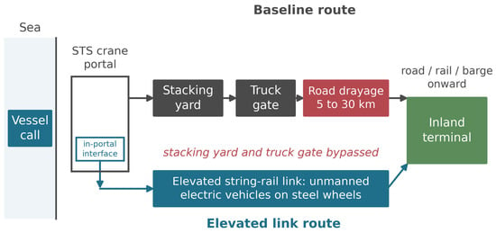
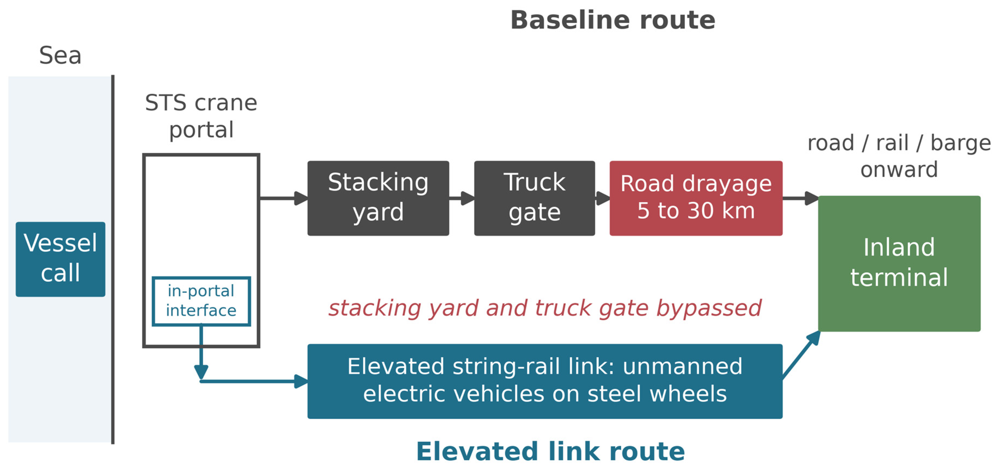
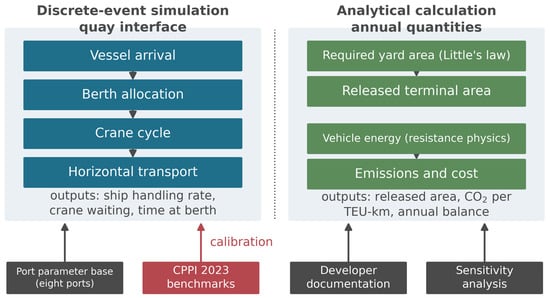
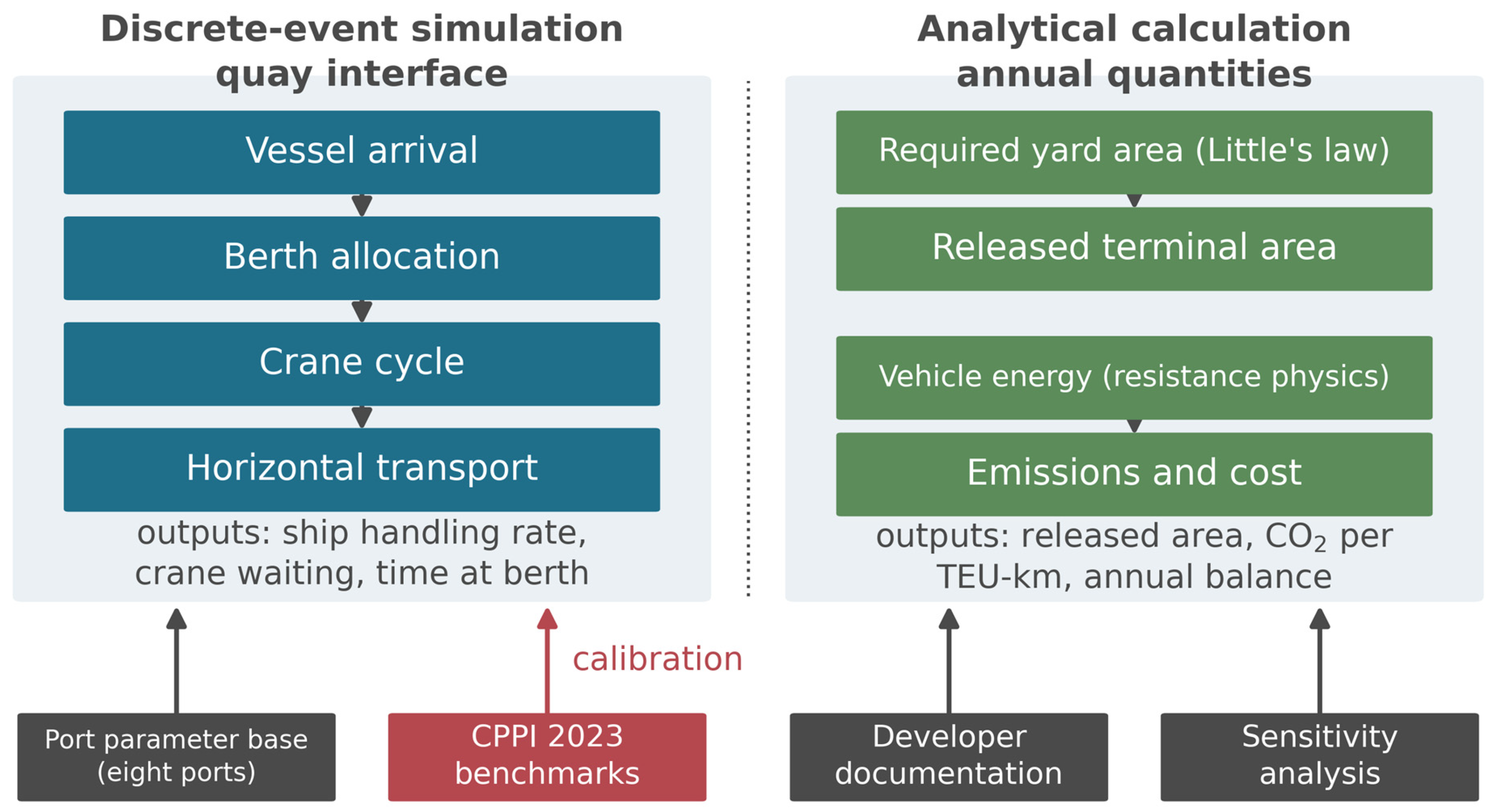
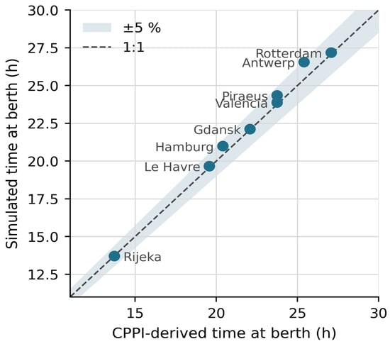
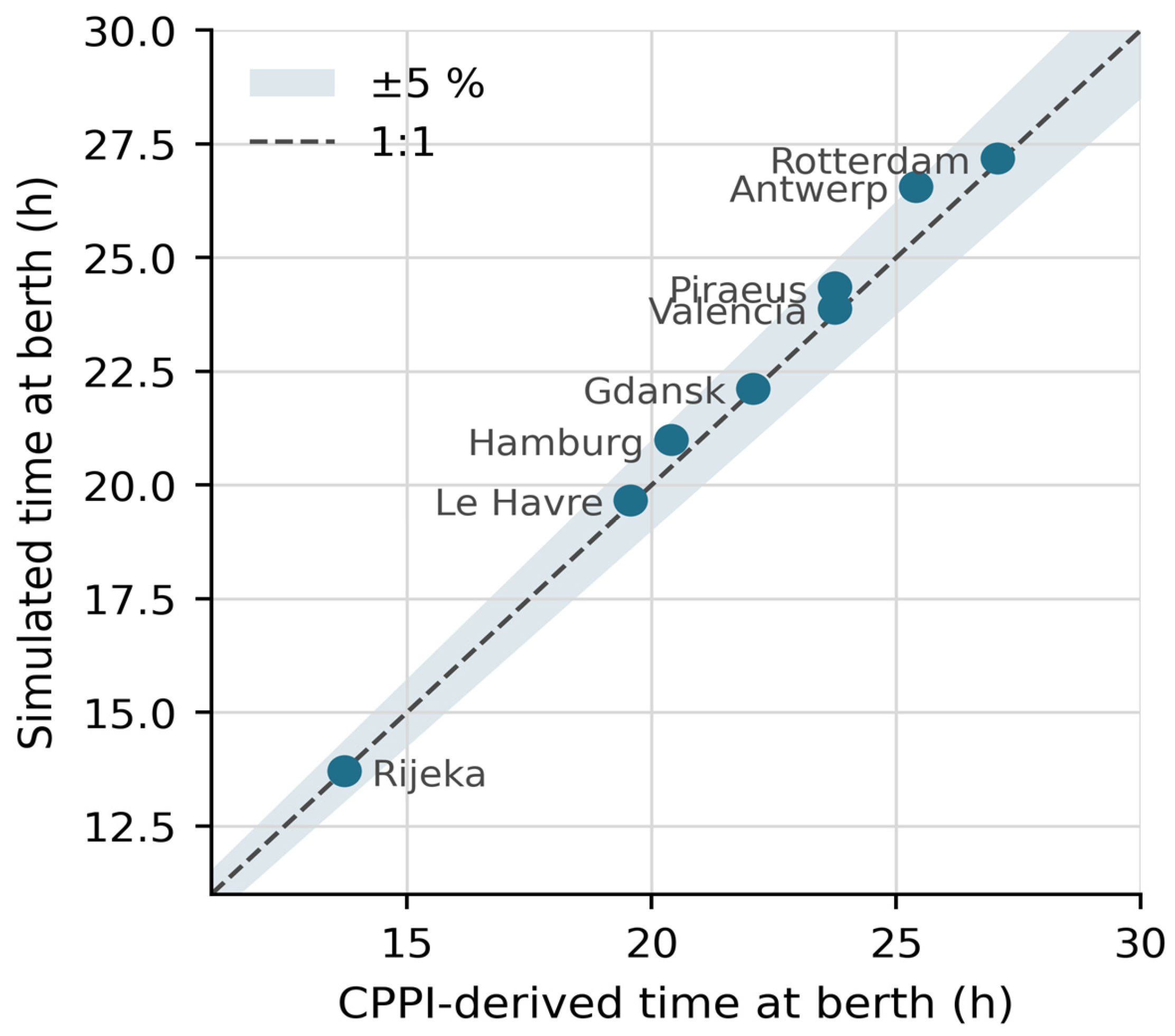
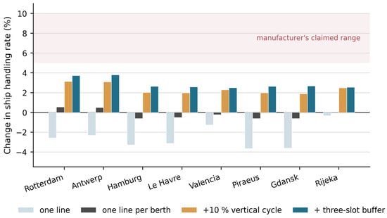
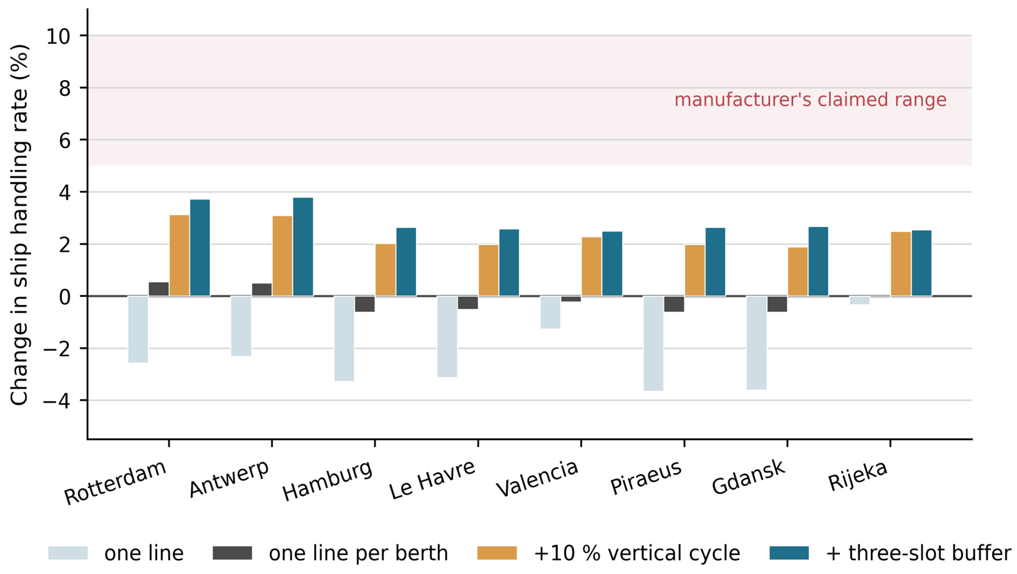
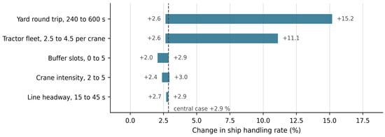
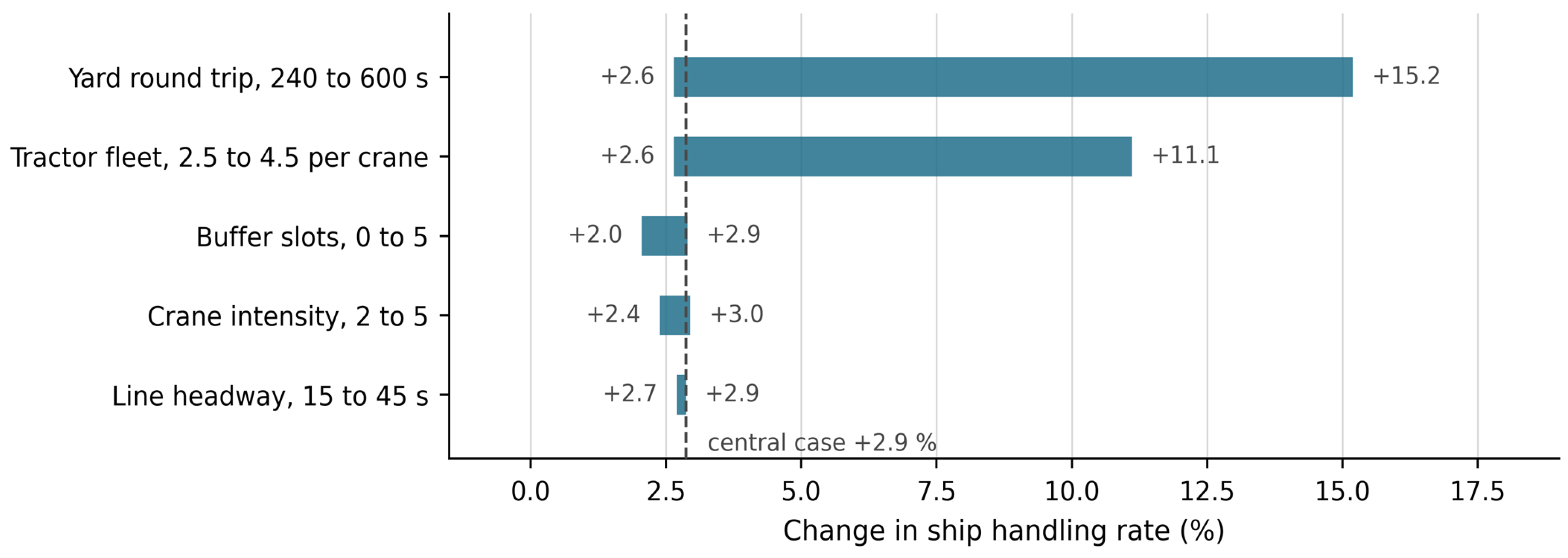
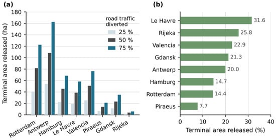
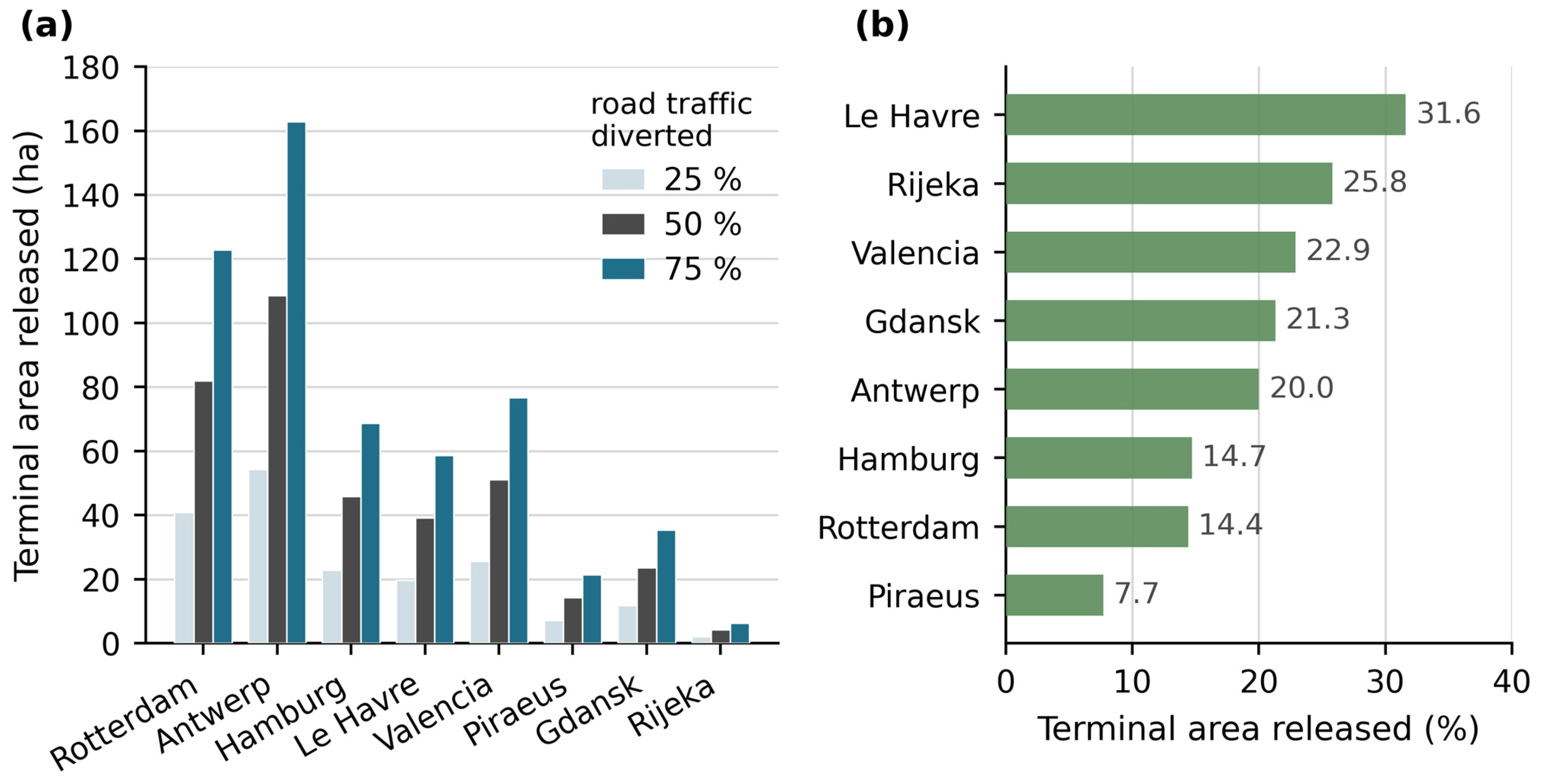
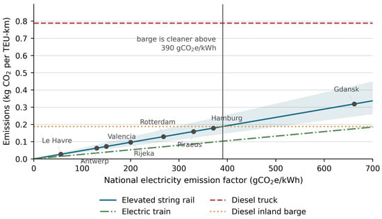
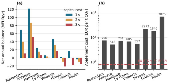
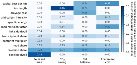
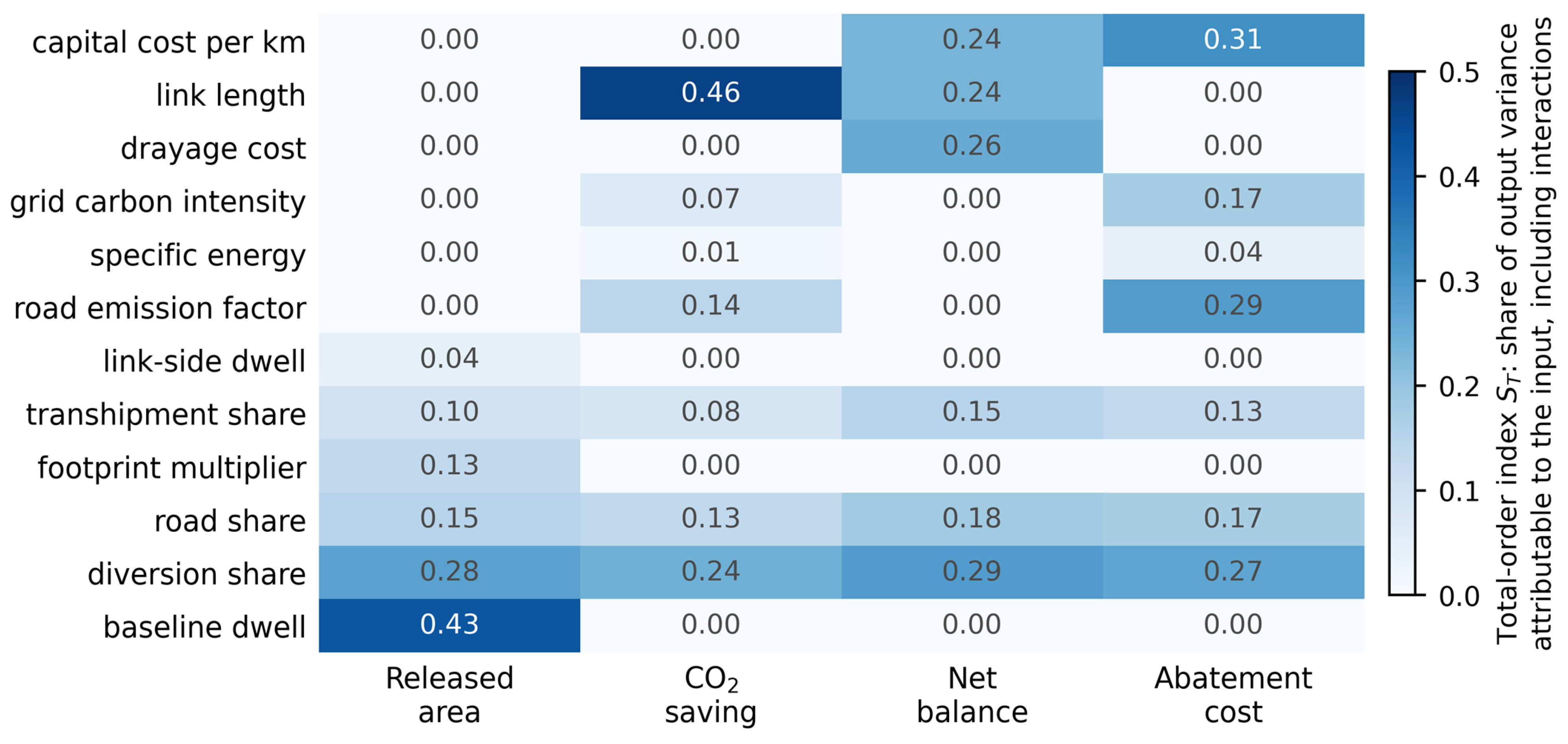

Disclaimer/Publisher’s Note: The statements, opinions and data contained in all publications are solely those of the individual author(s) and contributor(s) and not of MDPI and/or the editor(s). MDPI and/or the editor(s) disclaim responsibility for any injury to people or property resulting from any ideas, methods, instructions or products referred to in the content. |
© 2026 by the authors. Licensee MDPI, Basel, Switzerland. This article is an open access article distributed under the terms and conditions of the Creative Commons Attribution (CC BY) license.