Graph-Temporal Probabilistic Forecasting with Interpolation-Aware Data Representation

Abstract

This study proposes a method for probabilistic time-series forecasting on graphs incorporating interpolation (IA-GTPF)—a decision-tree-based ensemble approach that combines observation quality metrics, historical load dynamics, information on neighboring nodes, residual correction, quantile regression, and conformal calibration. The method’s performance was evaluated using the Open Power System Data Household dataset. Fixed time boundaries defined distinct periods for training, validation, calibration, and testing. Only information available at the time of forecasting was used as input, while graph weights and preprocessing parameters were determined solely based on the training set. A separate calibration period was used to adjust confidence interval boundaries without altering point forecasts. On the main test set, the IA-GTPF method demonstrated the following metrics for a 15-min forecast horizon: a Mean Absolute Error (MAE) of 0.9824 kW, a Root Mean Square Error (RMSE) of 2.5408 kW, and a Coefficient of Determination (R²) of 0.98947. For the 60-min horizon, the corresponding values were 1.3940 kW, 4.2017 kW, and 0.97122. The QuantileForest model showed a lower MAE for the 15-min horizon (0.9695 kW); however, IA-GTPF achieved the lowest RMSE and highest R² values. For the 60-min horizon, the IA-GTPF method demonstrated the lowest MAE and RMSE values among all evaluated models.

1. Introduction

Time series forecasting has become a central research topic in computer science, as modern Cyber–Physical systems continuously generate large volumes of heterogeneous temporal data. The rapid adoption of IoT devices, smart sensor technologies, and edge computing platforms has greatly increased the demand for accurate and robust forecasting models capable of handling complex multivariate sequences. Recent advances in deep learning have led to a variety of approaches for learning temporal representations. PatchTST employs patch-based representations to capture temporal dependencies [1], while TimesNet models temporal variations using multi-periodic representations [2]. TimeMixer integrates multi-scale temporal decomposition to capture patterns at different resolutions [3], whereas TSMixer utilizes an MLP-based architecture to mix temporal features [4]. iTransformer introduces an inverted attention mechanism to model dependencies between variables [5]. However, these approaches primarily focus on learning temporal representations rather than explicitly integrating dimension provenance, interpolation-aware features, and graph-based probabilistic forecasting. At the same time, graph neural networks have demonstrated a strong ability to model structural relationships between related observations, making graph temporal learning an increasingly important research direction in forecasting [6,7,8,9]. Furthermore, probabilistic forecasting has attracted considerable attention, as prediction intervals and uncertainty estimation provide more informative decision support than deterministic point forecasts in real-world applications [10,11,12].

Despite the progress made, forecasting based on heterogeneous time series from smart meters remains a challenging task. Individual measurement streams are often characterized by missing values, irregular sampling intervals, duplicate records, communication failures, and abrupt changes driven by consumer behavior or the operation of distributed energy resources. These characteristics reduce forecast reliability and often necessitate data interpolation or reconstruction prior to model training. Although recent studies have proposed increasingly sophisticated data reconstruction methods, reconstructed values are typically treated on par with original measurements, and the uncertainty associated with interpolation is ignored during feature engineering and probabilistic forecasting [13,14,15,16].

Large language models have recently been applied to spatiotemporal load forecasting, enabling the modeling of interdependencies among multiple energy consumers. Notably, the STDeepSeek model combines spatiotemporal modeling and continual learning techniques to forecast electricity demand at various electric vehicle charging stations, adapting to evolving load characteristics [17]. While this approach accounts for the dynamics of spatiotemporal dependencies, the present study focuses on integrating aspects such as measurement provenance, interpolation-aware feature representation, and probabilistic uncertainty calibration for heterogeneous smart meter data.

Existing graph-based time-series forecasting methods primarily focus on modeling structural connections and temporal dependencies between correlated series. Although such approaches account for interactions between entities, explicitly addressing measurement reliability and the provenance of reconstructed data remains a significant methodological challenge. Research on missing data recovery [13,14,15,16] primarily addresses the reconstruction of incomplete observations, whereas probabilistic forecasting methods [18,19,20] focus on forecast uncertainty and interval estimation. However, the comprehensive integration of feature representation incorporating interpolation, graph construction (performed only during the training phase), and probabilistic uncertainty calibration for heterogeneous smart meter data has not been sufficiently explored. These considerations motivated the development of the proposed IA-GTPF approach.

The scientific novelty lies in the integration of interpolation-aware data representation and graph-based probabilistic forecasting over time within a single learning architecture. Unlike recent studies that separately consider missing data imputation, graph-based forecasting, or uncertainty estimation, the proposed approach simultaneously models structural relationships, temporal dependencies, and interpolation robustness. This unified design allows the forecasting model to utilize the information contained in the reconstructed observations rather than discarding it after preprocessing, resulting in more robust probabilistic forecasting for heterogeneous smart meter data.

2. Materials and Methods

This study addresses the task of short-term net load forecasting for heterogeneous buildings using the publicly available Open Power System Data (OPSD) Household dataset (version dated 15 April 2020). This dataset comprises high-resolution smart meter readings from residential, public, and small industrial buildings in southern Germany; the data include aggregate figures for energy consumption and grid feed-in, photovoltaic generation, energy storage system operation, and the charging of electric vehicles and heat pumps. The availability of data with varying temporal resolutions and the explicit labeling of interpolated observations make this dataset suitable for evaluating forecasting methods that account for differences in data quality and building operating conditions. The study aims to develop and evaluate the IA-GTPF method for net load forecasting at 15- and 60-min intervals by integrating observation quality metrics, temporal dependencies, operating mode characteristics, and graph-based information. The methodology combines approaches such as causality-aware feature engineering, graph construction based solely on training data, ensemble decision-tree regression, ablation analysis, and comparison with baseline models. To prevent temporal information leakage, the experiments employ distinct chronological periods for training, validation, calibration, and testing, enabling independent assessment of point forecast accuracy and prediction interval quality. A description of the monitored buildings, available energy metering channels, and distributed energy resources is provided in Table S1 (Supplementary Material), while summary diagnostic data regarding intervals with extremely high positive values—identified during the preprocessing stage—are presented in Table S2.

2.1. Data Preprocessing and Leakage-Free Dataset Construction

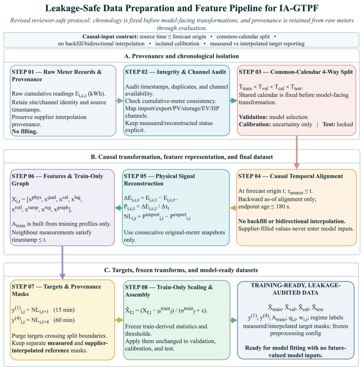
The IA-GTPF data preparation pipeline ensures chronological data isolation and prevents information leakage from the future. Model inputs are generated exclusively from observations available at the time forecasting begins, without employing “backward filling” or bidirectional interpolation methods. Data lineage information is preserved, allowing for the distinction between actual measurements and values interpolated by the data provider. The complete data preparation and feature engineering workflow is illustrated in Figure 1.

Figure 1. Leakage-safe data preparation and feature engineering pipeline for IA-GTPF.

Figure 1 shows the complete preprocessing flowchart that transforms raw cumulative smart meter measurements into a leak-proof dataset for model training. The workflow begins with defining the object, time, and measurement indices, followed by converting the cumulative energy readings into physically interpretable interval variables and constructing the target net load signal. Subsequent steps include data quality assessment, feature extraction with interpolation, temporal and statistical feature engineering, graph construction using only the training data, and chronological partitioning into training, validation, calibration, and test sets. The data preparation process is formally described by the following mathematical formulation, which defines the transformation of the original smart meter measurements into the final data set for modeling.

1. Indexing of objects, time and channels.

Let i denote the monitored object, t the time point, and c the measurement channel. The raw smart meter data are represented by cumulative energy measurements (1):

$$E_{i,t,c}^{\mathit{cum}}$$

(1)

where c may correspond to grid import, export, photovoltaic generation, battery storage, electric vehicle charging, heat pumps, or other available channels.

2. Conversion of cumulative measurements into interval variables. Because the original measurements are cumulative, the energy consumed or generated during each interval is obtained from consecutive readings (2):

$$\Delta E_{i,c,t}=E_{i,t,c}^{\mathit{cum}}-E_{i,t-1,c}^{\mathit{cum}}$$

(2)

Let Δτ_t denote the duration of the measurement interval in hours. The corresponding power-like representation is then calculated as (3):

$$P_{i,c,t}={\displaystyle \frac{\Delta E_{i,c,t}}{\Delta \mathrm{t}}}$$

(3)

These interval-based variables are subsequently used as physically interpretable representations of the available energy channels.

3. Construction of the net-load signal. The primary forecasting target is the net load of each monitored object. Based on the available grid import and export measurements, the net-load signal is defined as (4):

$$N{L}_{i,t}=P_{i,t}^{\mathrm{imp}}-P_{i,t}^{\exp }$$

(4)

when local generation and storage-related measurements are available, an auxiliary demand estimate is also constructed (5):

$$D_{i,t}=\mathrm{N}{L}_{i,t}+P_{i,t}^{\mathrm{PV}}+P_{i,t}^{\mathrm{bat}}$$

(5)

where $P_{i,t}^{\mathrm{PV}}$ and $P_{i,t}^{\mathrm{bat}}$ denote photovoltaic generation and the corresponding storage-related contribution, respectively. This quantity is used as an auxiliary physical feature rather than as the primary forecasting target.

4. Quantification of observation quality. Because the dataset contains missing and interpolated observations, the reliability of each observation is explicitly characterized. For each observation, the following quality indicators are considered: a missing-value indicator m_i,t, an interpolation indicator g_i,t, the normalized gap length g_i,t, and an abnormal-increment indicator a_i,t. The resulting quality score is defined as (6):

Q_i,t = 1 − (α_mm_i,t + α_qq_i,t + α_gg_i,t + α_aa_i,t)

(6)

where α_m,α_g,α_a—are non-negative weighting coefficients. The score is subsequently converted into an observation weight (7):

w_i,t = max(Q_i,t,ε)

(7)

where ε > 0 prevents zero-valued weights. The quality indicators and observation weights are retained as part of the data representation and are subsequently used by the proposed interpolation-aware forecasting framework.

5. Construction of forecasting targets. The forecasting problem is formulated for two horizons with a sampling interval of 15 min. For each object, the future net load is defined as (8):

$${\mathbf{y}}_{i,t}^{\left(\mathrm{h}\right)}=N{L}_{i,t+h},h\in \{1,4\}$$

(8)

This corresponds to forecasting with lead times of 15 and 60 min, respectively. Only observations available at or before the start of the forecasting period are used to construct the input representation. Information regarding the origin of the target data is preserved, making it possible to distinguish between directly measured values and reference values obtained via provider interpolation; this allows for the separate assessment of forecasting accuracy for each category of target data.

6. Chronological splitting. To prevent temporal data leakage between buildings with differing observation periods, the dataset is partitioned using common calendar cutoff dates. Nine key facilities with overlapping measurement periods are included in the forecast quality assessment. The same temporal boundaries are applied to all facilities, resulting in the formation of four non-overlapping subsets: training, validation, calibration, and test. The validation subset is used for model selection and the optimization of ensemble coefficients, while the independent calibration subset is intended for adjusting forecast confidence intervals. The test subset is used exclusively for the final performance evaluation (9):

$$T=T_{\mathit{train}}\cup T_{\mathit{val}}\cup T_{\mathit{cal}}\cup T_{\mathit{test}}, T_{\mathit{train}}<T_{\mathit{val}}<T_{\mathit{cal}}<T_{\mathit{test}}$$

(9)

The four non-overlapping subsets follow the chronological order of training, validation, calibration, and test. The training subset is used for model fitting, the validation subset for model selection, the calibration subset for prediction interval calibration, and the test subset exclusively for final performance evaluation.

7. Train-only imputation, encoding, and baseline-specific normalization. For each numerical feature x, normalization parameters are estimated exclusively from the training subset (10):

μ_x = meanT_train(x), σ_x = stdT_train(x)

(10)

and the normalized feature is obtained as (11):

$${\tilde{x}}_{i,t}={\displaystyle \frac{x_{i,t}-{\mu }_x}{{\sigma }_x+\epsilon }}$$

(11)

Missing values for numerical features are imputed using medians calculated solely from the training set, while categorical features are encoded using categories defined during the training phase. Standardization is not applied to decision tree-based IA-GTPF models. For linear and neural network base models requiring feature scaling, normalization parameters are determined exclusively from the training set and then applied without modification to the validation, calibration, and test sets.

2.2. Feature Engineering

Following the preprocessing procedure described in Section 2.1, a unified feature representation is constructed for each monitored object and forecasting time point. The feature engineering stage integrates physical, observation-quality, temporal, statistical, regime, and graph-based information. All features available at time t are constructed exclusively from observations at or before t, ensuring that no future information is introduced into the forecasting process. The physical feature block represents the current energy state of each monitored object. For each measurement channel c, the corresponding power-like value P_i,t,c obtained during preprocessing is used. To explicitly distinguish an unavailable channel from a measured zero value, an availability indicator is introduced (12):

A_i,t,c = II(P_i,t,c is observed)

(12)

The unified channel representation is then defined as (13):

$${\tilde{P}}_{i,t,c}=P_{i,t,c}{A}_{i,t,c}$$

(13)

The physical feature vector combines the available energy channels with the net-load and auxiliary demand variables (14):

$$x_{i,t}^{\mathit{phys}}=[{\tilde{P}}_{i,t,}, N{L}_{i,t},A_{i,t}]$$

(14)

To characterize the balance between imported and exported energy, an export activity indicator is additionally calculated as (15):

$${\mathit{R}}_{\mathit{i},\mathit{t}}^{\mathit{exp}}={\displaystyle \frac{{\mathit{P}}_{\mathit{i},\mathit{t}}^{\mathit{exp}}}{{\mathit{P}}_{\mathit{i},\mathit{t}}^{\mathit{imp}}+{\mathit{P}}_{\mathit{i},\mathit{t}}^{\mathit{exp}}+\mathit{\epsilon }}}$$

(15)

The relative photovoltaic contribution is represented by (16):

$${\mathit{R}}_{\mathit{i},\mathit{t}}^{\mathit{PV}}={\displaystyle \frac{{\mathit{P}}_{\mathit{i},\mathit{t}}^{\mathit{PV}}}{{\mathit{P}}_{\mathit{i},\mathit{t}}^{\mathit{PV}}+{\mathit{D}}_{\mathit{i},\mathit{t}}+\mathit{\epsilon }}}$$

(16)

These variables allow the model to distinguish between predominantly importing, exporting, locally generating, and mixed prosumer operating conditions. The preprocessing stage provides the quality indicators and observation weight described by Q_i,t and w_i,t. To retain information about the characteristics of missing or interpolated intervals, the quality feature vector is defined as (17):

$${\mathit{x}}_{\mathit{i},\mathit{t}}^{\mathit{qual}}=[{\mathit{m}}_{\mathit{i},\mathit{t}},{\mathit{q}}_{\mathit{i},\mathit{t}},{\mathit{g}}_{\mathit{i},\mathit{t}},{\mathit{a}}_{\mathit{i},\mathit{t}},{\mathit{Q}}_{\mathit{i},\mathit{t}},{\mathit{w}}_{\mathit{i},\mathit{t}}]$$

(17)

For long missing intervals, the gap length is transformed using a logarithmic representation (18):

$${\mathit{g}}_{\mathit{i},\mathit{t}}^{\mathit{log}}=\mathbf{log}(1+{\mathit{g}}_{\mathit{i},\mathit{t}})$$

(18)

This transformation preserves information about the duration of missing segments while reducing the influence of exceptionally long gaps. Calendar features are introduced to represent recurring daily, weekly, and seasonal patterns. Since direct numerical encoding of cyclic variables may create artificial discontinuities, periodic variables are represented using sine and cosine transformations (19):

$${\mathit{sin}}_{\mathit{k}}\left(\mathit{t}\right)=\mathbf{sin}\left({\displaystyle \frac{2\mathit{\pi t}}{{\mathit{T}}_{\mathit{k}}}}\right),{\mathit{cos}}_{\mathit{k}}\left(\mathit{t}\right)=\mathbf{cos}\left({\displaystyle \frac{2\mathit{\pi t}}{{\mathit{T}}_{\mathit{k}}}}\right)$$

(19)

where T_k denotes the corresponding period, such as a day, week, month, or year (20):

$${\mathit{x}}_{\mathit{i},\mathit{t}}^{\mathit{cal}}=[{\mathit{sin}}_{\mathit{day}},{\mathit{cos}}_{\mathit{day}},{\mathit{sin}}_{\mathit{week}},{\mathit{cos}}_{\mathit{week}},{\mathit{sin}}_{\mathit{season}},{\mathit{cos}}_{\mathit{season}},{\mathit{I}}_{\mathit{weekend}}]$$

(20)

Recent temporal dependencies are represented using lagged values of net load, demand, and selected physical channels. For a signal z_i,t and a predefined set of lags L, the lag representation is (21):

$${\mathit{x}}_{\mathit{i},\mathit{t}}^{\mathit{lag}}=[{\mathit{z}}_{\mathit{i},\mathit{t}-\mathit{l}}{]}_{\mathit{lϵL}}$$

(21)

To characterize local level and variability, rolling statistics are calculated over a set of historical windows W (22):

$${\mathit{x}}_{\mathit{i},\mathit{t}}^{\mathit{roll}}=[{\mathit{\mu }}_{\mathit{i},\mathit{t}}^{\left(\mathit{w}\right)},{\mathit{\sigma }}_{\mathit{i},\mathit{t}}^{\left(\mathit{w}\right)},{\mathit{z}}_{\mathit{i},\mathit{t}}^{\mathit{min},\left(\mathit{w}\right)},{\mathit{z}}_{\mathit{i},\mathit{t}}^{\mathit{max},\left(\mathit{w}\right)},{\mathit{z}}_{\mathit{i},\mathit{t}}^{\mathit{range},\left(\mathit{w}\right)}{]}_{\mathit{wϵW}}$$

(22)

where the corresponding statistics are calculated exclusively from observations available before or at time t. Changes in net load are represented using ramp features. The basic ramp is (23):

∆NL_i,t−, NL_i,t−1

(23)

The ramp feature block additionally includes absolute change, mean ramp activity, and local ramp variability (24):

$${\mathit{x}}_{\mathit{i},\mathit{t}}^{\mathit{ramp}}=\left[\mathbf{∆}\mathit{N}{\mathit{L}}_{\mathit{i},\mathit{t}},\left|\mathbf{∆}\mathit{N}{\mathit{L}}_{\mathit{i},\mathit{t}}\right|,\mathit{mean}(\mathbf{∆}\mathit{NL}),\mathit{std}(\mathbf{∆}\mathit{NL})\right]$$

(24)

These features capture short-term dynamics and rapid transitions that may not be adequately represented by the instantaneous net-load value alone. To explicitly represent qualitatively different operating conditions, four binary regime indicators are introduced: PV-active, export, weak-signal, and rapid-ramp regimes. They are combined into a single regime vector (25):

$${\mathit{r}}_{\mathit{i},\mathit{t}}=[\begin{array}{c}\begin{array}{c}\mathbb{I}\left({\mathit{P}}_{\mathit{i},\mathit{t}}^{\mathit{PV}}>{\mathit{T}}_{\mathit{PV}}\right)\\ \mathbb{I}\left(\mathit{N}{\mathit{L}}_{\mathit{i},\mathit{t}}<-{\mathit{T}}_{\mathit{exp}}\right)\\ \mathbb{I}\left(\left|\mathit{N}{\mathit{L}}_{\mathit{i},\mathit{t}}\right|<{\mathit{T}}_{\mathit{WS}}\right)\end{array}\\ \mathbb{I}\left(\left|\mathit{N}{\mathit{L}}_{\mathit{i},\mathit{t}}\right|>{\mathit{T}}_{\mathit{RAMP}}\right)\end{array}]$$

(25)

where T_PV,T_exp,T_WS,T_RAMP denote the corresponding operating thresholds. This representation enables the model to distinguish normal operation from PV-active, export, weak-signal, and rapidly changing conditions without introducing four separate mathematical definitions. In addition to temporal dependencies, the forecasting problem contains structural relationships between monitored objects. A graph is constructed exclusively from the training period to prevent information leakage from the validation and test periods. Let ${\mathit{s}}_{\mathit{i}}^{\mathit{train}}$ denote the training-period profile of object i. The similarity between objects i and j is defined as (26):

$${\mathit{S}}_{\mathit{ij}}={\displaystyle \frac{{\mathit{s}}_{\mathit{i}}^{\mathit{train}}\ast {\mathit{s}}_{\mathit{j}}^{\mathit{train}}}{\left|\left|{\mathit{s}}_{\mathit{i}}^{\mathit{train}}\right|\right|\left|\left|{\mathit{s}}_{\mathit{j}}^{\mathit{train}}\right|\right|+\mathit{\epsilon }}}$$

(26)

A sparse adjacency matrix is then constructed by retaining the \(K\) most similar training objects for each node (27):

A_ij = II(j∈ N_k(i))S_ij

(27)

where N_k(i) denotes the set of selected neighbors of object i. For an arbitrary signal z_i,t, the graph-based neighborhood representation is (28):

$${\mathit{G}}_{\mathit{i},\mathit{t}}\left(\mathit{z}\right)={\displaystyle \frac{{\sum }_{\mathit{j}\in {\mathit{N}}_{\mathit{k}}\left(\mathit{i}\right)}{\mathit{A}}_{\mathit{i},\mathit{j}}{\mathit{z}}_{\mathit{j},\mathit{t}}}{{\sum }_{\mathit{j}\in {\mathit{N}}_{\mathit{k}}\left(\mathit{i}\right)}{\mathit{A}}_{\mathit{i},\mathit{j}}+\mathbf{\in }}}$$

(28)

The graph-based neighborhood representation in Equation (28) assumes a centralized forecasting scenario in which contemporaneous smart meter measurements from neighboring buildings are available before the forecast for building i is issued. At each forecasting origin t, only measurements available at or before t are used to predict the net load at t + h, where h corresponds to 15 or 60 min. This operational scenario assumes timely data transmission from neighboring buildings. Communication delays and asynchronous meter reporting are not explicitly evaluated in the present study. The graph deviation is calculated as (29):

$${\mathit{D}}_{\mathit{i},\mathit{t}}^{\mathit{graph}}\left(\mathit{z}\right)={\mathit{z}}_{\mathit{i},\mathit{t}}-{\mathit{G}}_{\mathit{i},\mathit{t}}(\mathit{z})$$

(29)

The graph feature block therefore provides both neighborhood context and the deviation of the target object from its structurally similar peers. All feature blocks are concatenated into a unified representation (30):

$${\mathit{X}}_{\mathit{i},\mathit{t}}=[{\mathit{x}}_{\mathit{i},\mathit{t}}^{\mathit{phys}},{\mathit{x}}_{\mathit{i},\mathit{t}}^{\mathit{qual}},{\mathit{x}}_{\mathit{i},\mathit{t}}^{\mathit{cal}},{\mathit{x}}_{\mathit{i},\mathit{t}}^{\mathit{lag}},{\mathit{x}}_{\mathit{i},\mathit{t}}^{\mathit{roll}},{\mathit{x}}_{\mathit{i},\mathit{t}}^{\mathit{ramp}},{\mathit{r}}_{\mathit{i},\mathit{t}},{\mathit{x}}_{\mathit{i},\mathit{t}}^{\mathit{graph}}]$$

(30)

The resulting representation combines the instantaneous physical state, observation reliability, recurring temporal patterns, recent dynamics, operating regimes, and cross-object structural information. All components are constructed without access to future observations and are subsequently provided to the proposed IA-GTPF architecture described in Section 2.3. The complete feature dictionary, including feature groups, data types, and their use in the proposed forecasting framework, is provided in Table S3 (Supplementary Materials).

2.3. Proposed IA-GTPF Architecture

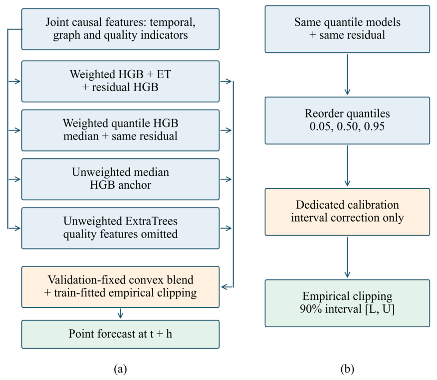
Figure 2 illustrates the trainable tree branches and the coefficients fixed after validation. A residual correction is applied to the deterministic and quantile components, while independent calibration adjusts only the interval boundaries. The individual outputs are a point forecast, the median quantile, and an uncertainty interval.

Figure 2. Overview of the proposed forecasting framework: (a) point forecasting and ensemble blending pipeline; (b) quantile forecasting and prediction interval calibration pipeline.

IA-GTPF combines six types of trainable components: weighted gradient boosting, weighted ExtraTrees, residual correction boosting, three quantile regressors, an unweighted median regressor, and an additional ExtraTrees model that excludes quality features. Temporal and graph representations serve as input features rather than hidden neural layers. Missing numerical values are replaced with training-set medians, and categorical features are encoded based on training-set categories. Standardization is not applied to the tree-based models; it is used only for linear and neural network comparisons. First, HGB and ExtraTrees models are evaluated on quality-weighted training data, and the coefficient for their combination is selected based on validation MAE (31):

$${\widehat{\mathit{y}}}_{\mathit{i},\mathit{t},\mathit{h}}^{\mathbf{base}}={\mathit{\lambda }}_{\mathit{h}}{\mathit{f}}_{\mathbf{HGB},\mathit{h}}\left({\mathbf{X}}_{\mathit{i},\mathit{t}}\right)+\left(1-{\mathit{\lambda }}_{\mathit{h}}\right){\mathit{f}}_{\mathbf{ET},\mathit{h}}\left({\mathbf{X}}_{\mathit{i},\mathit{t}}\right)$$

(31)

In-sample residuals are generated for the selected combination. A separate HGB is trained to predict these residuals using weights $w_{i,t}(1 + 0.75z{w}_{s_i,t})$. The use of in-sample residuals carries a risk of overfitting this branch; its utility is verified via independent ablation (32):

$$e_{i,t,h}=y_{i,t}^{\left(h\right)}-{\widehat{y}}_{i,t,h}^{\mathrm{base}}, {\widehat{e}}_{i,t,h}=g_h\left({\mathrm{X}}_{i,t}\right), {\widehat{y}}^{\det }={\widehat{y}}^{\mathrm{base}}+\widehat{e}$$

(32)

Three quantile HGB models minimize the weighted quantile loss function. A common residual correction is added to each quantile, and the boundaries are ordered before constructing the interval (33):

ρ_τ(e) = max{τe,(τ − 1)e},  τ ∈ {0.05,0.50,0.95}

(33)

The final point forecast is a convex combination of the adjusted deterministic forecast, the adjusted median regressor, the unweighted median regressor, and an additional ensemble tree. The coefficients are selected from a grid with a step of 0.1 based solely on validation. The point forecast is not identified with the median of interval (34):

$$\widehat{y}={\pi }_d{\widehat{y}}^{\det }+{\pi }_q\left(f_{0.50}+\widehat{e}\right)+{\pi }_a{f}_{\mathrm{anchor}}+{\pi }_r{f}_{\mathrm{robust}}, {\pi }_k\ge 0, {\sum }_k{\pi }_k=1$$

(34)

Once the regressors and coefficients are fixed, a separate calibration period is used solely to adjust the bounds. Simply enabling or disabling this adjustment does not alter the point forecast. Empirical range constraints, estimated based on training targets, are verified separately and are not referred to as known physical power limits. The ensemble coefficients selected on the validation set for the 15-min and 60-min forecasting horizons across five random initializations are reported in Table S5 (Supplementary Materials).

After training the regression branches and tuning the ensemble coefficients on the validation set, the predictive models are fixed. Subsequently, an independent calibration set is used exclusively to determine the adjustment of the prediction interval boundaries. For each observation in the calibration set, the conformity score is determined according to formula (35):

$$s_n=\max \{{\widehat{q}}_{0.05.n}-y_n, y_n-{\widehat{q}}_{0.95.n}, 0\}$$

(35)

where s_n is the nonconformity score for the n-th observation from the calibration set; y_n is the corresponding observed net load; ${\widehat{q}}_{0.05.n}$ and ${\widehat{q}}_{0.95.n}$ are the predicted lower and upper quantile bounds, respectively; and n is the index of the calibration observation. This score characterizes the extent to which the observed value falls outside the predicted interval and equals zero if the observation falls within that interval. The calibration adjustment is calculated from the empirical distribution of the conformity scores (36):

$$\widehat{\delta }=Q_{\left[\left(N+1\right)\left(1-\alpha \right)\right]/N} (\left\{s_n{\}}_{n=1}^N\right), \alpha =0.1$$

(36)

where $\widehat{\delta }$ is the correction obtained via conformal calibration; Q_p(∙) is the empirical quantile operator for level p, N is the number of observations in the calibration sample; α is the nominal non-coverage level (set to 0.10 for a 90% prediction interval), and [∙] is the ceiling function. This correction is estimated solely based on nonconformity scores obtained from an independent calibration sample. The resulting calibrated prediction interval is (37):

$$I_{i,t+h}=[{\widehat{q}}_{0.05,i,t+h}-\widehat{\delta },{\widehat{q}}_{0.95,i,t+h}+\widehat{\delta } ]$$

(37)

where I_i,t+h is the calibrated prediction interval for building i at time t + h, i is the building index, t is the forecast start time, h is the forecast horizon, ${\widehat{q}}_{0.05,i,t+h}$ and ${\widehat{q}}_{0.95,i,t+h}$ are the predicted lower and upper quantiles of the net load, respectively, and $\widehat{\delta }$ is the conformal calibration adjustment estimated from an independent calibration sample. The resulting interval is formed by subtracting $\widehat{\delta }$ from the lower quantile and adding it to the upper quantile. Conformal calibration modifies only the boundaries of the prediction interval and does not affect the final point prediction. Object-specific empirical constraints on output values, when employed, are estimated solely based on target values from the training set and are not interpreted as known physical power limits. The detailed implementation settings of IA-GTPF, including temporal lags, graph construction criteria, observation-quality coefficients, operating-regime thresholds, regression hyperparameters, and calibration settings, are provided in Table S4 (Supplementary Materials).

The IA-GTPF model was configured separately for 15-min and 60-min forecasting horizons. Temporal features were derived from lagged observations (with lags of 1, 2, 4, 8, 16, 32, 92, 95, and 96 time steps) and sliding windows of 4, 16, and 96 steps, based on a 15-min base resolution. The graph was constructed exclusively from training data using positive Pearson correlation values; a maximum of four neighbors per building was permitted, and each potential connection required at least 500 joint observations in the training set. Self-loops (connections of a node to itself) were excluded, and the resulting adjacency weights were row-normalized.

Observation reliability was accounted for via a constrained quality metric using coefficients of 0.45, 0.35, and 0.20 for missing data in measured channels, unavailability of current net load data, and the presence of anomalous increments, respectively. Corresponding observation weights were further adjusted based on the duration of the current data gap (using a 0.10 coefficient). Threshold values for operating modes were determined from the training data: small net load changes were identified using the 35th percentile, sharp changes using the 85th, and photovoltaic system operating modes using the 30th and 70th percentiles. These thresholds were fixed prior to model application during the validation, calibration, and testing stages.

The core forecasting component consisted of a combination of HistGradientBoosting (HGB) and ExtraTrees regressors, with weights determined by data quality. Two HGB configuration variants were considered: 180 and 240 boosting iterations, learning rates of 0.05 and 0.035, maximum leaf counts of 31 and 45, and L₂ regularization coefficients of 0.05 and 0.10, respectively. The primary ExtraTrees regressor employed 70 trees with a maximum depth of 18 and a minimum of four observations per leaf. Residual correction was performed using a separate HGB regressor (90 iterations, learning rate 0.04, 23 leaves, L₂ coefficient 0.08). The probabilistic component comprised three quantile regressors based on gradient boosting on decision trees (HGB), corresponding to quantile levels of 0.05, 0.50, and 0.95.

Model selection and uncertainty calibration were carried out using separate chronological data splits. Ensemble coefficients were selected from a grid of values with a step of 0.1 by minimizing the MAE on the validation set. Subsequently, the selected coefficients were fixed prior to model evaluation on the test set. Confidence interval adjustment (with a nominal coverage level of 90%) was performed using an independent calibration set, without altering the point forecasts. The experiments involved five random initialization variants (11, 23, 37, 53, and 71) and five evaluation time periods. Full implementation parameters and ensemble coefficients selected during the validation stage are presented in Tables S4 and S5, respectively (in the Supplementary Materials).

3. Results

3.1. Data Characterization and Feature Validation

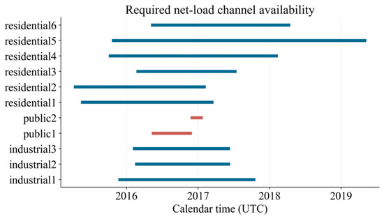
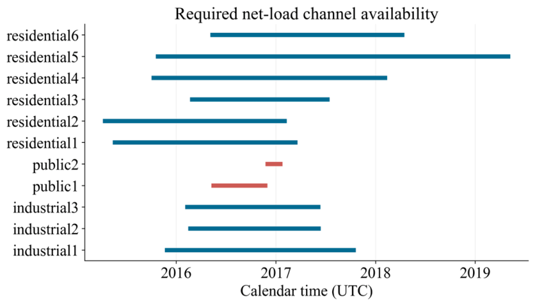
The buildings under observation exhibit non-uniformity in temporal coverage resulting from differences in the availability of measurement data from smart meters. To characterize these differences, the data-recording periods for the respective net load measurement channels were analyzed for all 11 buildings. Figure 3 illustrates the temporal availability of these channels for residential, industrial, and public buildings.

Figure 3. Temporal availability of required net-load measurement channels across the monitored buildings.

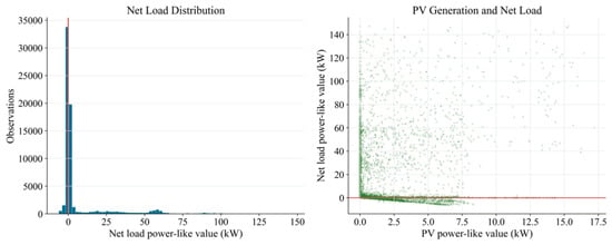
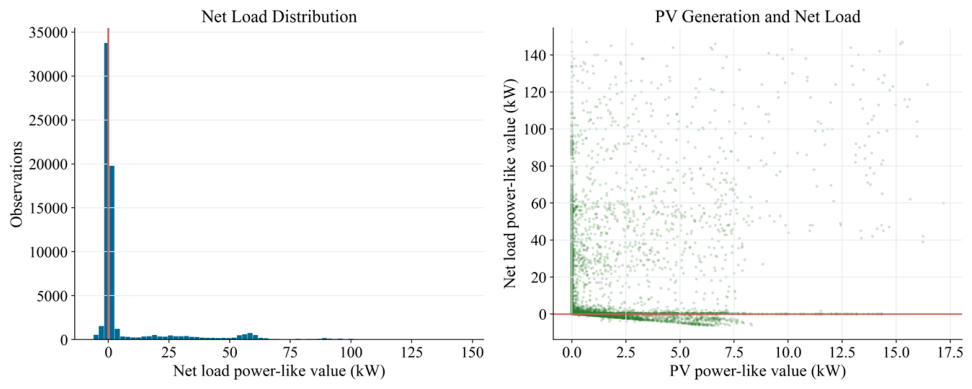
Figure 3 illustrates the uneven temporal coverage of data across 11 monitored sites, comprising six residential buildings, three industrial facilities, and two public buildings. The available measurements span various periods between 2015 and 2019, with residential buildings exhibiting longer observation periods compared to industrial and public sites. These disparities result in a temporally unbalanced dataset, necessitating a split strategy based on a unified calendar schedule to prevent the leakage of temporal information between sites. Consequently, uniform calendar split dates are applied to all sites included in the forecast quality assessment; this ensures that training data consistently precedes the validation, calibration, and testing periods across the entire dataset used for evaluation. Although all 11 sites were considered during the initial data characterization, the forecast assessment based on the unified calendar schedule is limited to nine primary sites (six residential buildings and three industrial facilities) with overlapping measurement periods. The two public buildings were excluded from this assessment because their temporal coverage was insufficient to accommodate the selected training, validation, calibration, and testing intervals. Figure 4 shows the distribution of the constructed target net load value after converting cumulative energy measurements into values similar to interval power values. The distribution is centered around zero, indicating a predominance of periods of low load operation, while the pronounced positive tail reflects episodes of high grid electricity imports.

Figure 4. Net load distribution and connection of PV generation with power-like network exchange values.

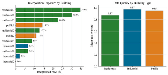
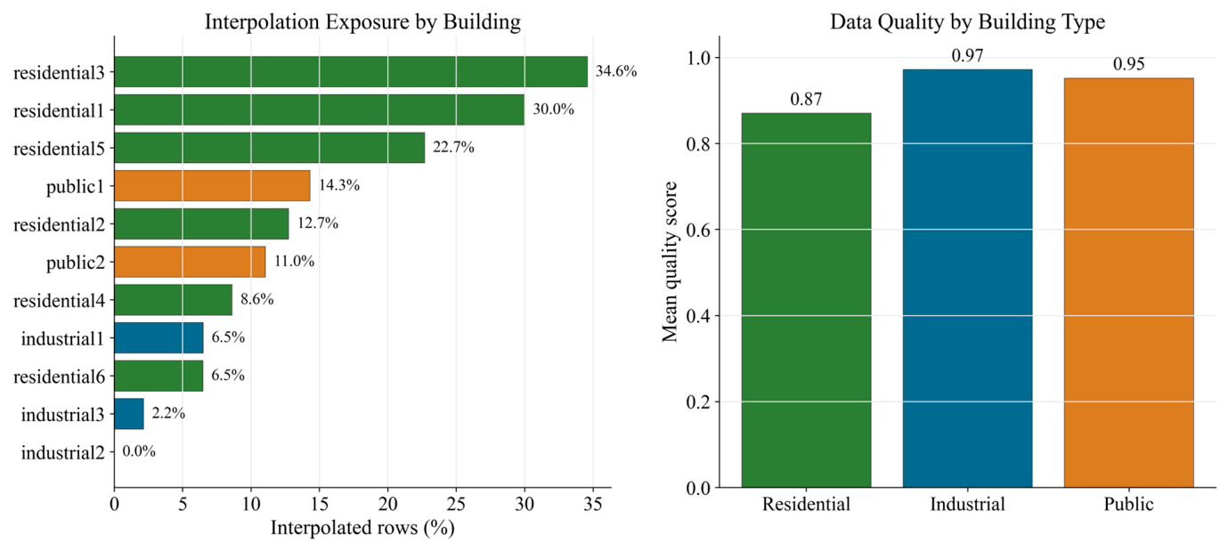
Figure 4 presents the statistical characteristics of the constructed net load target. Most observations are concentrated in the range of approximately 0–5 kW, indicating the prevalence of low-load operating conditions in the dataset. The distribution exhibits a pronounced positive tail, reaching nearly 160 kW, confirming the presence of rare but significant demand peaks. In contrast, negative net load values are relatively rare and typically remain around −5 kW, reflecting episodic electricity exports from consumer-producer buildings. The scatterplot also shows that PV generation spans a range of approximately 0–17.5 kW, while high PV generation is generally associated with lower net load values, although significant spread remains due to fluctuations in electricity demand. Figure 5 shows the distribution of interpolated exposure for individual buildings, as well as the average data quality estimates for different building categories.

Figure 5. Interpolation load by objects and average data quality by building type.

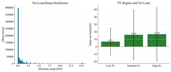
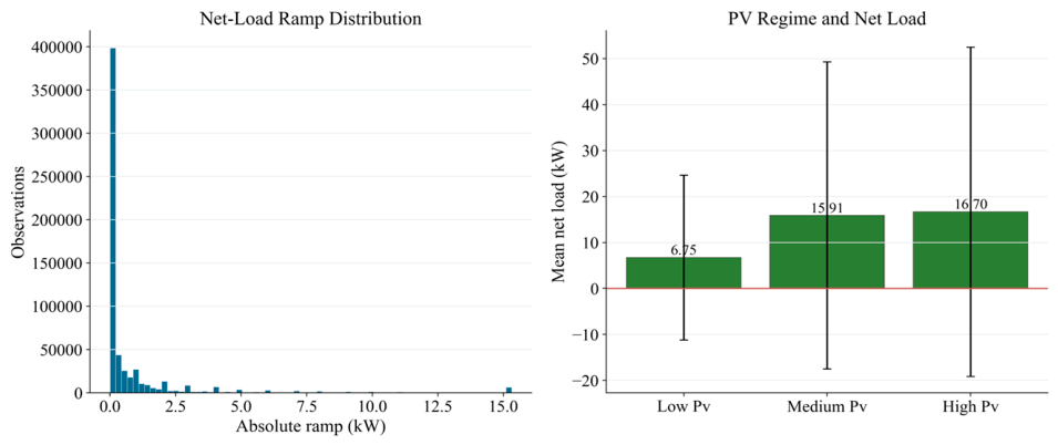
Figure 5 shows significant variability in interpolation requirements across the monitored buildings. The proportion of interpolated observations ranges from 0.0% for industrial buildings2 to 34.6% for residential buildings3, with residential buildings generally demonstrating higher interpolation rates than industrial and public buildings. Despite these differences, the average data quality remains consistently high across all building categories, with average quality scores of 0.87 for residential, 0.97 for industrial, and 0.95 for public buildings. These results indicate that missing observations are concentrated in a limited number of buildings, while the overall dataset maintains a high level of measurement reliability. Figure 6 shows the distribution of net load change values and the relationship between PV generation modes and the corresponding average net load levels.

Figure 6. Distribution of net load ramp events and average net load under different PV modes.

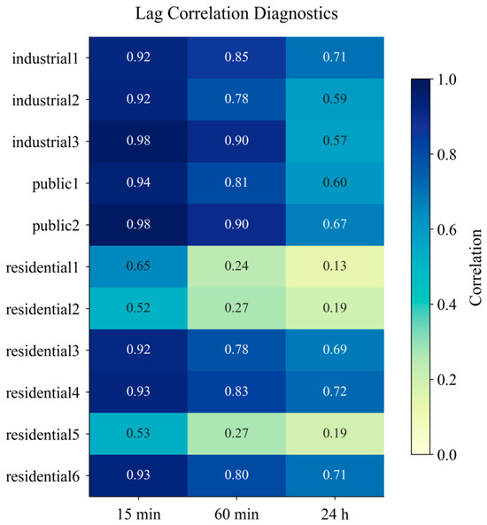
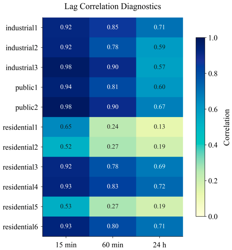
Figure 6 shows that the net load dynamics are dominated by small changes, with the vast majority of power surges concentrated below 1 kW, while larger surges are relatively rare, reaching approximately 16 kW. Analysis of the PV system operating mode further reveals a gradual increase in the average net load from 6.75 kW at low PV system power to 15.91 kW and 16.70 kW at medium and high PV system power, respectively. However, significant errors indicate significant variability within each operating mode, reflecting the combined effects of PV generation and the high variability of household electricity demand. Figure 7 shows a heat map of the correlation of the current net load with its lag values on three time scales: 15 min, 60 min and 24 h.

Figure 7. Diagnostics of lag correlation of net load by objects and time horizons.

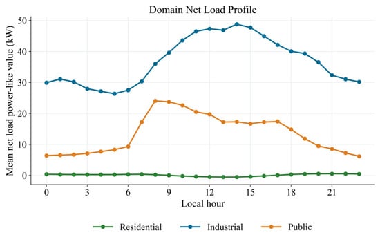
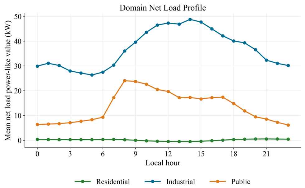
The results show that the industrial and public objects exhibit pronounced temporal inertia. For example, for industrial1, the correlation is 0.92 at a lag of 15 min, 0.85 at 60 min, and 0.71 at 24 h. Similar persistence is observed for industrial2, industrial3, public1, and public2. This means that for these objects, recent history and daily frequency predict future net load well, making lag features and rolling statistics methodologically sound. The residential group exhibits more heterogeneous behavior. Residential3, residential4, and residential6 maintain high correlation even at a daily lag, while residential1, residential2, and residential5 exhibit rapid decay: for example, residential1 decreases from 0.65 at 15 min to 0.13 at 24 h, and residential2 from 0.52 to 0.19. This indicates more irregular household dynamics, weak daily repeatability, and an increased role of local regimes, data quality, PV/export states, and ramp features. Figure 8 shows average daily net load profiles for residential, industrial and public buildings, illustrating the differences in energy consumption patterns depending on building category.

Figure 8. Daily profile of average net load by object type.

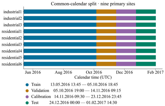
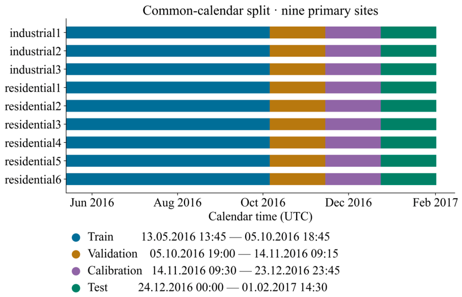
Figure 8 shows different patterns of daily electricity consumption in three building categories. Industrial buildings exhibit the highest and most stable demand, increasing from approximately 30 kW at night to a daytime peak of approximately 49 kW around 1:00–3:00 p.m., and then gradually decreasing in the evening. Public buildings exhibit a distinct consumption profile during working hours: the net load increases sharply after 7:00 a.m., reaching approximately 24 kW around 8:00 a.m., and steadily decreases after the workday ends to less than 7 kW late in the evening. In contrast, residential buildings maintain consistently low net load values, remaining close to 0 kW throughout the day with only minor fluctuations. These distinct temporal patterns indicate that building type strongly influences the dynamics of electricity demand, supporting the use of time-graph representations capable of capturing the heterogeneous daily behavior of interconnected buildings. To ensure an evaluation free from data leakage when dealing with buildings that have varying observation periods, a partitioning strategy based on a unified calendar schedule was employed. Nine primary facilities with overlapping measurement periods were selected, and identical time boundaries were established for all buildings. The resulting training, validation, calibration, and testing periods are shown in Figure 9.

Figure 9. Partitioning the nine main sites into training, validation, calibration, and test subsamples using a unified calendar schedule.

Figure 9 illustrates the data partitioning based on a unified schedule for nine buildings, comprising six residential and three industrial facilities. The training period spans from 13 May to 5 October 2016, followed by validation (5 October to 14 November 2016), calibration (14 November to 23 December 2016), and testing (24 December 2016, to 1 February 2017) phases. Identical temporal boundaries are applied to all nine buildings, ensuring that the training data precedes the validation, calibration, and testing periods for each facility. This partitioning eliminates temporal overlap between the training and evaluation periods and provides a consistent basis for analyzing prediction accuracy within the unified schedule protocol.

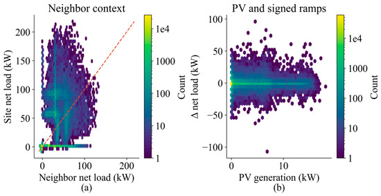
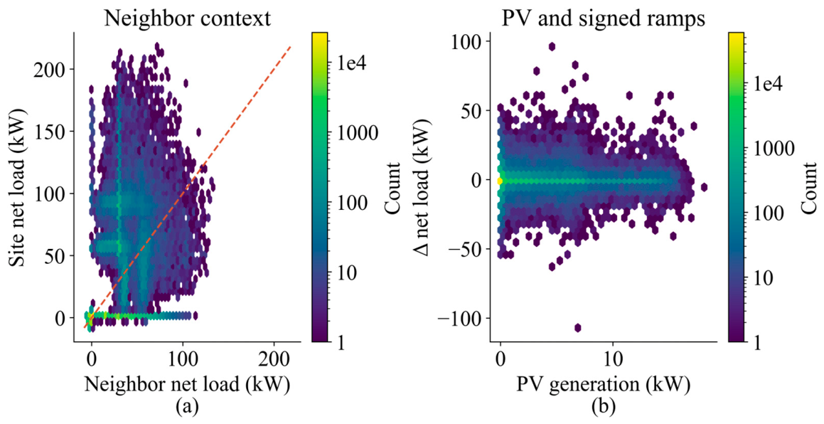
Figure 10 compares the current net load with the causally accessible neighboring context and load variations under different generation conditions. Significant dispersion indicates that the aggregate of neighbors does not substitute for individual characteristics. The observed relationship does not, in itself, establish a causal dependency between the buildings.

Figure 10. Adjacency graph and local network load dynamics: (a) neighbor net load versus site net load; (b) PV generation versus signed net-load ramps.

Figure 10a shows a significant spread in local net load values for similar load levels at neighboring sites. For instance, with a load of approximately 50 kW at a neighboring site, the local net load ranges from values close to zero to over 200 kW; this indicates that measurements at neighboring sites alone are insufficient to reliably characterize local demand. Figure 10b shows that net load variations (taking the sign into account) cluster around the zero mark across the entire observed range of photovoltaic power generation, although in some instances deviations exceed ±50 kW.

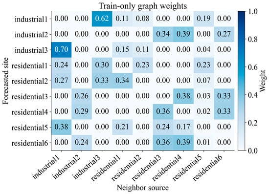
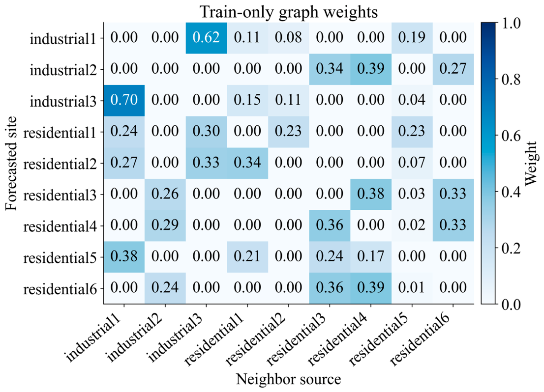
Figure 11 shows the weights used: the diagonal is zero, and the rows are normalized. The selection of neighbors and the normalization process can render the matrix asymmetric, even though the initial correlation is symmetric. These statistical relationships define the model’s context and are not interpreted as electrical connections.

Figure 11. Matrix of normalized weights of the training graph without self-loops.

The heatmap displays graph weights (calculated exclusively from the training set) assigned to neighboring entities for each target entity. These weights are sparse and vary across entities, indicating that the graph does not assign equal importance to all neighboring sources. For instance, the entity ‘industrial1’ assigns the highest weight to ‘industrial3’ (0.62), whereas ‘industrial3’ assigns the highest weight to ‘industrial1’ (0.70). Residential entities exhibit more dispersed connections: some receive information from both neighboring residential and industrial entities. Since the weights were estimated solely based on training data, constructing the graph does not require information from the validation or testing periods.

3.2. Comparative Performance Evaluation of IA-GTPF

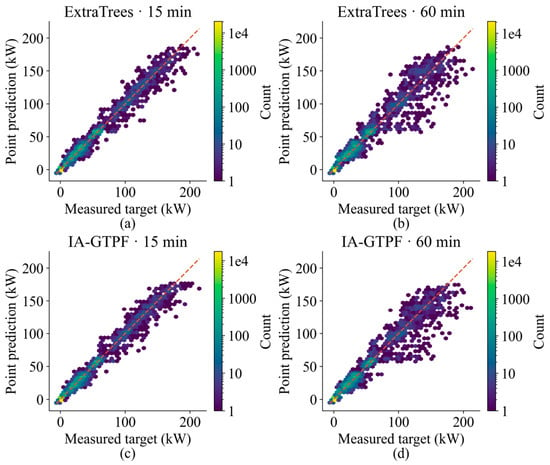
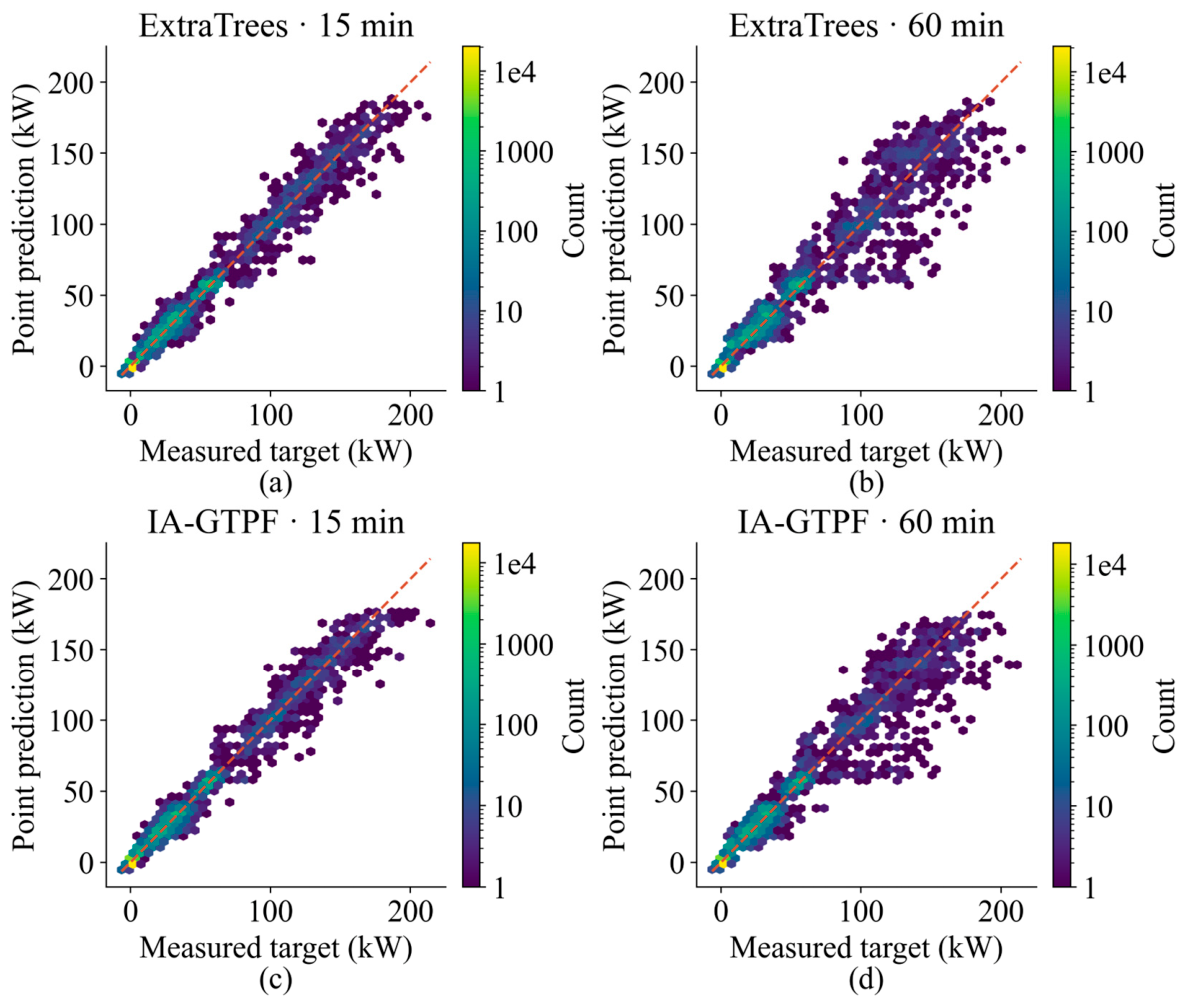
Figure 12 compares measured net load values with point forecasts obtained using the ExtraTrees and IA-GTPF methods for forecast horizons of 15 and 60 min. Panels (a) and (b) show the ExtraTrees results, while panels (c) and (d) present the corresponding IA-GTPF forecasts. The dashed diagonal line represents perfect agreement between measured and predicted values, and the color scale indicates the number of observations.

Figure 12. Comparison of measured and predicted net load for IA-GTPF and ExtraTrees: (a) ExtraTrees at 15-min resolution; (b) ExtraTrees at 60-min resolution; (c) IA-GTPF at 15-min resolution; (d) IA-GTPF at 60-min resolution.

For both forecasting horizons, the results of the IA-GTPF and ExtraTrees models cluster near the diagonal, particularly at low net load values. As the load increases, the dispersion grows, a trend that is more pronounced for the 60-min horizon. At the 60-min horizon, the IA-GTPF model demonstrates a higher degree of alignment with the diagonal, consistent with its lower RMSE compared to ExtraTrees (4.2017 kW vs. 4.4590 kW). Both models tend to underestimate values for certain high-load observations, highlighting the difficulty of predicting high net load levels.

Table 1 compares the point forecasting accuracy of the IA-GTPF model and baseline models on the main test set of measured target values for forecast horizons of 15 and 60 min. Performance is evaluated using MAE, RMSE, and the R². The test set contains 32,527 measured target values for each run. Where applicable, results are presented as the mean and standard deviation calculated from five random initializations.

Table 1. Point-forecast accuracy on the main test set with measured targets at the 15-min and 60-min forecasting horizons.

Model	15 min: MAE, kW	15 min: RMSE, kW	15 min: R2	60 min: MAE, kW	60 min: RMSE, kW	60 min: R2
IA-GTPF	0.9824 ± 0.0032	2.5408 ± 0.0042	0.98947 ± 0.00003	1.3940 ± 0.0078	4.2017 ± 0.0153	0.97122 ± 0.00021
QuantileForest	0.9695 ± 0.0068	2.5473 ± 0.0068	0.98942 ± 0.00006	1.4817 ± 0.0072	4.4265 ± 0.0318	0.96806 ± 0.00046
ExtraTrees	1.0013 ± 0.0262	2.5542 ± 0.0380	0.98936 ± 0.00032	1.5836 ± 0.0520	4.4590 ± 0.0909	0.96758 ± 0.00133
Conformalized ExtraTrees	1.0013 ± 0.0262	2.5542 ± 0.0380	0.98936 ± 0.00032	1.5836 ± 0.0520	4.4590 ± 0.0909	0.96758 ± 0.00133
RandomForest	1.0243 ± 0.0110	2.5677 ± 0.0164	0.98925 ± 0.00014	1.4837 ± 0.0075	4.2517 ± 0.0251	0.97053 ± 0.00035
QuantileHGB	1.0312	2.6734	0.98834	1.4571	4.3584	0.96904
Persistence	1.0338	2.6691	0.98838	1.5131	4.6793	0.96431
HGB	1.0560	2.6491	0.98855	1.5099	4.3109	0.96971
GRU-lite	1.0834 ± 0.0230	2.6808 ± 0.0548	0.98827 ± 0.00048	1.5581 ± 0.0426	4.3642 ± 0.0585	0.96895 ± 0.00084
Ridge	1.0879	2.5716	0.98921	1.8196	4.2341	0.97078
GraphTemporalMLP-lite	1.1969 ± 0.0330	2.8111 ± 0.0610	0.98711 ± 0.00056	1.6572 ± 0.0368	4.4207 ± 0.0446	0.96814 ± 0.00064
TCN-lite	1.2149 ± 0.0560	2.8628 ± 0.1190	0.98661 ± 0.00112	1.7177 ± 0.0670	4.5939 ± 0.1115	0.96558 ± 0.00166
PatchTST-lite	1.2437 ± 0.0456	2.9254 ± 0.0655	0.98604 ± 0.00062	1.6698 ± 0.0238	4.4559 ± 0.0579	0.96763 ± 0.00084
STGCN	1.3156 ± 0.0713	3.2524 ± 0.1862	0.98270 ± 0.00198	1.8529 ± 0.0921	4.9146 ± 0.2228	0.96056 ± 0.00348
DLinear-lite	1.6097 ± 0.6898	3.9297 ± 2.0743	0.96920 ± 0.03600	1.9841 ± 0.6382	5.4041 ± 1.7746	0.94829 ± 0.03815
Seasonal Persistence	2.6343	9.5179	0.85225	2.6360	9.5210	0.85223

To assess the robustness of the observed differences, a pairwise comparison of MAE values was conducted using confidence intervals and the Diebold–Mariano test with the Holm correction for multiple comparisons (Table S7). On the primary test set, the difference between IA-GTPF and ExtraTrees at the 15-min forecast horizon was not statistically significant (ΔMAE = 0.0189 kW, 95% CI: −0.0150 to 0.0622 kW; adjusted p = 1.0000). In contrast, at the 60-min horizon, the difference was statistically significant (ΔMAE = 0.1896 kW, 95% CI: 0.1199 to 0.2754 kW; adjusted p = 0.0004). These results indicate that the performance advantage over ExtraTrees is more robust at the longer forecast horizon. The sensitivity of the pairwise MAE differences and their confidence intervals to the temporal block length is further illustrated in Figure S1 (Supplementary Materials), which compares the results obtained using daily and seven-day evaluation blocks. Building-level forecasting performance across the nine evaluated buildings at both forecasting horizons is presented in Figure S3 (Supplementary Materials). Additional forecasting results for the two public buildings evaluated in separate cohorts are reported in Table S8 (Supplementary Materials). Table 2 presents the results not as a long list of individual algorithms, but as a comparison of methodological families. The proposed framework demonstrates competitive performance across the evaluated forecasting horizons and metrics. The closest families are the randomized tree ensemble and bagging tree ensemble, confirming the high competitiveness of tree-based methods with well-designed lag, rolling, graph, and quality features.

Table 2. Summary of the best representatives by model family.

Family	Best Representative	MAE	RMSE	R2	sMAPE
Proposed framework	IA-GTPF	1.1369	3.3393	0.9845	36.9496
Randomized tree ensemble	ExtraTreesRegressor	1.1652	3.3685	0.9843	39.1799
Bagging tree ensemble	RandomForestRegressor	1.1818	3.4418	0.9836	38.8641
Probabilistic boosting	Quantile HistGradientBoosting	1.2091	3.5871	0.9822	37.4283
Gradient boosting	HistGradientBoostingRegressor	1.2249	3.4966	0.9831	42.8681
Linear model	Ridge	1.3718	3.5152	0.9829	80.2916
Feed-forward neural model	MLPRegressor	1.3907	3.4250	0.9837	66.3943
Modern-lite graph-temporal NN	GraphTemporalMLP-lite	1.6422	3.7579	0.9804	85.7571
Modern-lite sequence model	DLinear-lite	1.7070	3.8324	0.9796	106.7192
Modern-lite recurrent model	GRU-lite	2.0370	5.4109	0.9594	104.3276
Modern-lite temporal convolution	TCN-lite	2.1532	4.0783	0.9769	99.9914
Modern-lite Transformer	PatchTST-lite	3.0532	5.7793	0.9537	109.8544

Probabilistic boosting demonstrates strong sMAPE but is inferior in absolute errors. This is important for the discussion: probabilistic setup alone does not guarantee better point forecasting unless combined with graph-temporal and interpolation-aware components. Linear and feed-forward neural models show that simply using the entire feature space without specialized quality mechanisms, graph, and mode correction is insufficient to achieve better results. Modern-lite sequence baselines in this configuration were inferior to table ensembles. To assess the contribution of individual components to the forecasting accuracy of the IA-GTPF model, an ablation study was conducted for forecast horizons of 15 and 60 min. The full-featured model was compared against configurations that excluded specific elements: graph features, observation quality information, residual correction, conformal calibration, small-change features, or quantile branches within the point-forecasting ensemble. One of the additional configurations utilized data from neighboring buildings with a 15-min time lag. Table 3 presents the Mean Absolute Error (MAE) and Standard Deviation (SD) for each configuration across all examined time intervals. Lower MAE values indicate higher point-forecast accuracy, while SD characterizes error variability across the various evaluation stages.

Table 3. IA-GTPF ablation assessment.

Configuration	15 min: Mean ± SD	60 min: Mean ± SD
Full IA-GTPF	1.2614 ± 0.1640	1.7595 ± 0.2768
No graph	1.2615 ± 0.1593	1.7590 ± 0.2762
No quality features or weights	1.2608 ± 0.1642	1.7654 ± 0.2727
No residual correction	1.2623 ± 0.1632	1.7610 ± 0.2769
No conformal correction	1.2614 ± 0.1640	1.7595 ± 0.2768
No small-change features	1.2651 ± 0.1606	1.7724 ± 0.2789
No quantile branches in the point mixture	1.2938 ± 0.1838	1.8539 ± 0.3465
Neighboring data with a 15-min lag	1.2616 ± 0.1659	1.7647 ± 0.2828

Ablation analysis results show that removing quantile branches leads to the most significant increase in MAE: from 1.2614 to 1.2938 kW (a 2.57% increase) for the 15-min forecast horizon and from 1.7595 to 1.8539 kW (a 5.37% increase) for the 60-min horizon. Excluding features representing minor changes increases MAE by 0.0037 and 0.0129 kW, respectively. Removing graph features, quality information, or the residual correction mechanism has a relatively minor impact (≤0.0059 kW), whereas disabling conformal correction does not alter point forecast accuracy. The effect of excluding residual correction across different temporal evaluation periods is illustrated in Figure S2 (Supplementary Materials). The variation in the direction and magnitude of the error changes indicates that the contribution of this component depends on the evaluation period. The performance of probabilistic forecasting was evaluated on the primary test set of actual values for both forecast horizons. Table 4 presents metrics for empirical coverage, mean interval width, absolute calibration error, interval score (IS), and weighted interval score (WIS₉₀) for the IA-GTPF model and baseline probabilistic forecasting models. In addition to the original and independently calibrated IA-GTPF intervals, the comparison includes intervals obtained after empirical range restriction and after rolling recalibration.

Table 4. Probabilistic forecasting performance on the main test set of measured targets at the 15-min and 60-min horizons.

Horizon	Model/Procedure	Coverage	Mean Interval Width, kW	Calibration Error	IS, kW	WIS90, kW
15 min	IA-GTPF: original quantiles	0.9117	13.6283	0.0117	15.1326	0.8432
15 min	IA-GTPF: independent calibration	0.9117	13.6283	0.0117	15.1326	0.8432
15 min	IA-GTPF: calibration and range restriction	0.9101	13.5522	0.0101	15.0983	0.8421
15 min	IA-GTPF: rolling recalibration	0.9343	13.7502	0.0343	15.0028	0.8389
15 min	QuantileForest	0.9162	5.5174	0.0162	6.9240	0.5540
15 min	QuantileHGB	0.9069	13.7145	0.0069	15.2282	0.8513
15 min	Conformalized ExtraTrees	0.9236	7.3078	0.0236	12.7337	0.7582
60 min	IA-GTPF: original quantiles	0.9252	14.6536	0.0252	17.6914	1.0786
60 min	IA-GTPF: independent calibration	0.9252	14.6536	0.0252	17.6914	1.0786
60 min	IA-GTPF: calibration and range restriction	0.9252	14.6525	0.0252	17.6903	1.0786
60 min	IA-GTPF: rolling recalibration	0.9418	14.8362	0.0418	17.6163	1.0761
60 min	QuantileForest	0.9254	7.7082	0.0254	9.5911	0.8136
60 min	QuantileHGB	0.9052	14.6459	0.0052	17.6993	1.0757
60 min	Conformalized ExtraTrees	0.9079	9.8032	0.0079	21.0481	1.2295

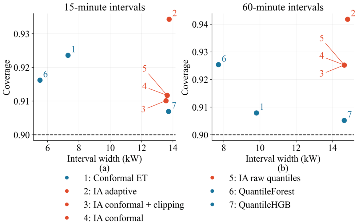
Independent calibration did not alter the initial IA-GTPF intervals for any of the forecast horizons, as the calculated conformal correction value was zero. Following empirical range restriction, the coverage rate was 0.9101 for the 15-min horizon and 0.9252 for the 60-min horizon. Rolling recalibration increased coverage to 0.9343 and 0.9418, respectively; however, it resulted in wider intervals and a greater deviation from the nominal 90% coverage level. The QuantileForest method yielded lower interval scores compared to the range-restricted IA-GTPF across both horizons: 6.9240 versus 15.0983 kW (15 min) and 9.5911 versus 17.6903 kW (60 min). Thus, the point-forecasting accuracy of the IA-GTPF method does not guarantee superior probabilistic performance across all evaluated metrics.

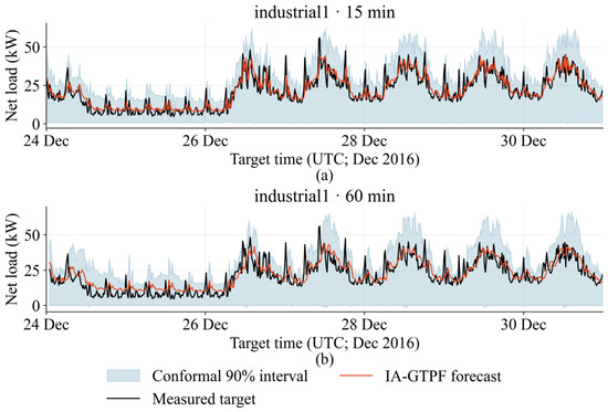
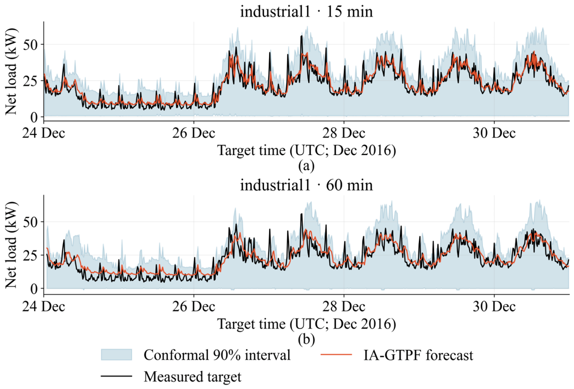
Figure 13 presents the forecasting results for the *industrial1* facility over the selected test period. For both forecasting horizons, the point forecasts obtained using the IA-GTPF method generally track the measured net load profile, capturing recurring peaks and demand fluctuations. The shaded 90% confidence intervals represent forecast uncertainty and widen during periods of significant load volatility. With the 60-min forecasting horizon, more pronounced deviations from measured values are observed during times of abrupt demand changes. These plots clearly illustrate the forecasting results and interval behavior for a single building; they should not be interpreted as evidence of achieving 90% empirical coverage across the entire test dataset.

Figure 13. IA-GTPF forecast and 90% intervals for two horizons: (a) 15-min forecasting horizon; (b) 60-min forecasting horizon.

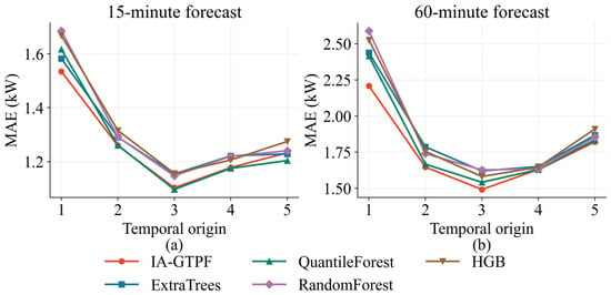
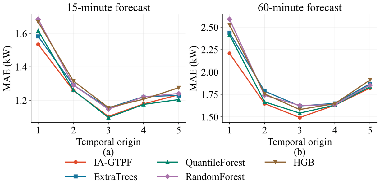
Figure 14 shows the average MAE across initializations for each temporal validation. The relative ranking of the models varies across periods. IA-GTPF exhibits the lowest average error across the five validations among the methods presented; however, this does not imply superiority in every single period or statistical superiority over every competitor.

Figure 14. Comparison of the main models based on the results of five consecutive temporal validation checks: (a) 15-min forecast; (b) 60-min forecast.

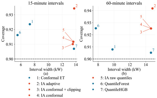
Figure 14 presents the results of the rolling-origin evaluation for 15-min and 60-min forecast horizons across five consecutive validation periods. Forecasting errors vary from period to period, reflecting changes in underlying load characteristics and operating conditions. The IA-GTPF method demonstrates a low average MAE across all periods considered, although its relative performance compared to individual baseline models varies depending on the specific origin point. Generally, errors are higher for the 60-min forecast horizon than for the 15-min horizon. The numerical results of the five rolling-origin evaluations are provided in Table S6. The table reports the mean MAE and standard deviation for IA-GTPF and the principal baseline models at both forecasting horizons, allowing the variability in forecasting performance across temporal evaluation periods to be assessed. Figure 15 illustrates the trade-off between interval width and empirical coverage, allowing for an assessment of the impact of independent conformal calibration, empirical range restriction, and rolling recalibration.

Figure 15. Empirical coverage versus mean interval width of 90% prediction intervals for IA-GTPF and probabilistic baseline models at the (a) 15-min and (b) 60-min forecasting horizons.

As shown in Figure 15, independent conformal calibration does not alter the original IA-GTPF intervals for any of the forecast horizons; consequently, the points corresponding to the original and calibrated configurations coincide. At the 15-min horizon, empirical range restriction slightly reduces the interval width (from 13.6283 to 13.5522 kW), while the coverage level drops from 0.9117 to 0.9101. Rolling recalibration raises the coverage level to 0.9343 but simultaneously increases the interval width to 13.7502 kW. A similar pattern is observed at the 60-min horizon: rolling recalibration increases coverage from 0.9252 to 0.9418 and interval width from 14.6536 to 14.8362 kW. The QuantileForest method yields significantly narrower intervals compared to IA-GTPF at both horizons while maintaining an empirical coverage level above the nominal 90% value.

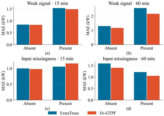
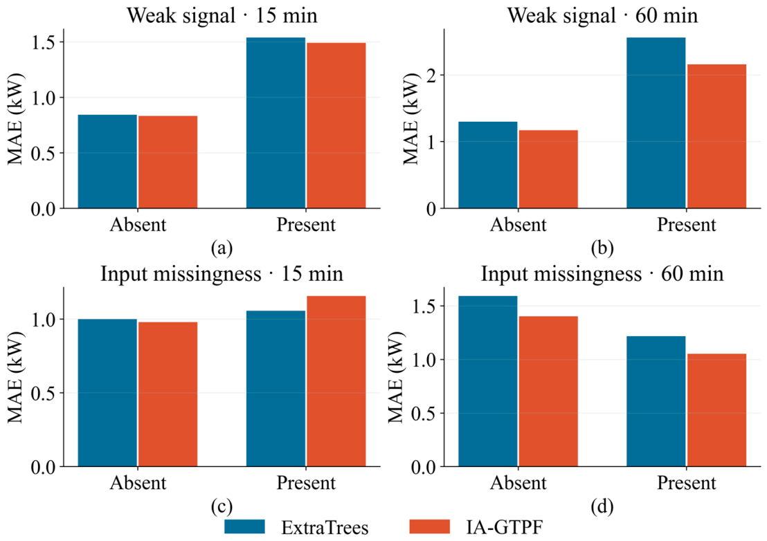
Figure 16 compares the MAE of the IA-GTPF and ExtraTrees methods under various data conditions for forecast horizons of 15 and 60 min. Panels (a) and (b) present results for observations with and without weak signals, while panels (c) and (d) compare observations with and without missing input values.

Figure 16. Forecasting errors associated with small-change regimes and input unavailability: (a) weak-signal regime at 15-min resolution; (b) weak-signal regime at 60-min resolution; (c) input missingness at 15-min resolution; (d) input missingness at 60-min resolution.

The presence of weak signals is associated with higher MAE values for both models across both forecasting horizons. At the 15-min horizon, errors increase from approximately 0.85 to 1.50 kW; at the 60-min horizon, they rise from approximately 1.2–1.3 to 2.1–2.5 kW. The impact of missing input data varies by horizon: at the 15-min horizon, MAE increases slightly in the presence of missing data, whereas at the 60-min horizon, MAE is lower for observations with missing input data. Overall, the IA-GTPF model demonstrates lower MAE values compared to ExtraTrees across all groups considered, although at the 15-min horizon, its error is slightly higher for observations with missing input data. These results indicate that the presence of weak signals complicates the forecasting task, while the relationship between missing input data and error magnitude is less straightforward.

4. Discussion

Experimental results demonstrate that the IA-GTPF model achieves competitive accuracy in short-term net load forecasting by integrating observation quality information, temporal and graph features, residual correction, and probabilistic forecasting within a decision-tree-based ensemble framework. An evaluation protocol employing a unified calendar schedule, causal input data generation, and graph weight determination exclusively during the training phase was implemented to minimize temporal information leakage and ensure the comparability of evaluation results across all buildings studied.

A comparative analysis shows that the performance of IA-GTPF depends on the forecasting horizon and the evaluation metric used. For a 15-min forecasting horizon, the proposed model yielded the following results: MAE = 0.9824 kW, RMSE = 2.5408 kW, and R² = 0.98947. Although the QuantileForest model achieved a slightly lower MAE (0.9695 kW), IA-GTPF demonstrated the lowest RMSE and highest R² values among all models evaluated. At a 60-min horizon, IA-GTPF metrics were: MAE = 1.3940 kW, RMSE = 4.2017 kW, and R² = 0.97122; notably, the MAE was 4.33% lower than that of the QuantileHGB model. These results indicate that the proposed approach yields more significant accuracy improvements as the forecasting horizon increases, although the extent of this advantage varies depending on the specific metrics and competing models.

Ablation analysis (the step-by-step exclusion of components) provides deeper insight into the contribution of individual model elements. Excluding quantile branches from the point forecasting ensemble resulted in a 2.57% increase in MAE (for the 15-min horizon) and a 5.37% increase (for the 60-min horizon), confirming their importance for forecast accuracy. Excluding features characterized by weak signals also led to increased forecasting errors for both horizons. Conversely, excluding graph-based features or observation quality features caused only minor changes in MAE, with the nature of this impact varying depending on the forecasting horizon. The findings indicate that the contribution of individual components depends on forecasting conditions, and their inclusion does not always improve point forecast accuracy across all experimental scenarios. As expected, omitting conformal calibration did not affect point forecasting errors, since this procedure adjusts confidence interval bounds rather than the point forecasts themselves. The probabilistic assessment highlights the importance of analyzing uncertainty estimates independently of point forecast accuracy. The initial IA-GTPF forecast intervals yielded empirical coverage levels of 0.9117 and 0.9252 for the 15-min and 60-min horizons, respectively. Independent conformal calibration did not alter these intervals, as the calculated adjustment value was zero. Rolling recalibration increased coverage levels to 0.9343 and 0.9418, respectively, but resulted in wider intervals and greater deviation from the nominal 90% coverage level. Furthermore, the QuantileForest method produced narrower intervals and lower interval quality metric values for both horizons. The results demonstrate that a higher empirical coverage level does not necessarily indicate better calibration or more informative uncertainty estimates. They also show that the point forecasting performance of the IA-GTPF model does not guarantee superiority in terms of probabilistic characteristics across all evaluated metrics.

The results of the ablation study indicate that incorporating the graph component yields only a marginal improvement in forecasting performance. Although graph-based features capture information regarding neighboring buildings, their exclusion does not lead to a significant drop in overall forecast accuracy. This suggests that temporal and physical characteristics, along with measurement quality metrics, already account for a substantial portion of the information required for short-term net load forecasting. Consequently, the graph component should be viewed as a source of supplementary contextual information rather than a primary determinant of the model’s predictive efficacy. Its contribution may depend on the degree of inter-building correlation and the availability of reliable measurement data from neighboring sites. Further research is needed to identify the conditions under which the use of graph-based information provides more tangible benefits.

The updated experimental protocol addresses several methodological challenges associated with forecasting based on heterogeneous smart meter data. Uniform timeframes were established for all nine buildings participating in the main evaluation phase, and model inputs were derived exclusively from information available at the time of forecasting. Graph weights and preprocessing parameters were determined solely using the training set, while a separate calibration period was used to adjust intervals. These measures minimize identified sources of temporal information leakage. However, independent calibration does not guarantee adherence to the nominal coverage level in the presence of temporal dependencies or distribution shifts between calibration and testing periods, highlighting the need for further research into adaptive uncertainty estimation methods.

Several limitations of this study should be noted. The primary analysis focused on nine buildings from a single geographic region with overlapping data collection periods, limiting the generalizability of the results to larger, more heterogeneous smart grid networks. Furthermore, the relatively small number of monitored sites precludes a full assessment of graph connectivity patterns under more complex operating conditions. The results obtained from lightweight neural network baselines should be viewed in the context of the specific computational parameters and hyperparameter settings used, rather than as evidence of fundamental limitations inherent to deep learning methods.

Consequently, future research should focus on external validation using larger and geographically diverse datasets, adaptive graph construction methods, and a more detailed analysis of observation quality in the presence of missing data. Integrating additional meteorological and behavioral variables, combined with conformal calibration techniques adapted for time series, could enhance forecasting reliability and the accuracy of uncertainty estimation under changing operating conditions.

5. Conclusions

This study proposes IA-GTPF, a decision-tree-based ensemble method for short-term probabilistic net load forecasting. The method integrates observation quality metrics, temporal and graph-based features, residual correction, quantile regression, and conformal calibration. Performance evaluation was conducted using the Open Power System Data Household dataset, following a unified scheduling protocol that entails distinct periods for training, validation, calibration, and testing. To mitigate the risk of temporal information leakage, input data generation relied on causal relationships, and graph construction was performed exclusively during the training phase.

On the primary test dataset, for a 15-min forecasting horizon, the IA-GTPF model achieved the following results: MAE = 0.9824 kW, RMSE = 2.5408 kW, and R² = 0.98947. For the 60-min horizon, the corresponding metrics were 1.3940 kW, 4.2017 kW, and 0.97122. Although the QuantileForest model demonstrated a slightly lower MAE for the 15-min horizon, IA-GTPF exhibited the lowest RMSE and highest R² among all evaluated models. For the 60-min horizon, the proposed method yielded the lowest MAE and RMSE values, demonstrating competitiveness across both forecasting horizons.

Ablation analysis revealed that quantile branches made the most significant contribution to point forecasting accuracy, whereas the impact of graph-based features and observation quality metrics was less pronounced and varied depending on the forecasting horizon. Probabilistic assessment also demonstrated that independent conformal calibration does not alter the original confidence intervals, whereas rolling recalibration improves empirical coverage at the cost of widening intervals and increasing the deviation from the nominal coverage level. The QuantileForest model yielded narrower intervals and lower interval score values across both horizons, highlighting the need to separately evaluate point forecast accuracy and the quality of probabilistic estimates.

Overall, the study results confirm the merit of integrating data preparation methods incorporating causal relationships, observation quality information, and graph-temporal features into a unified forecasting system. However, the evaluation was limited to data from nine buildings in a single geographic region, and the contribution of individual components varied depending on forecasting conditions. Future research will focus on validation using larger and geographically diverse datasets, adaptive graph construction, and time-series-specific uncertainty calibration to enhance forecasting reliability under changing operating conditions.

References

- Nie, Y.; Nguyen, N.H.; Sinthong, P.; Kalagnanam, J. A time series is worth 64 words: Long-term forecasting with transformers. arXiv 2022, arXiv:2211.14730. [Google Scholar] [CrossRef] [Scilit]
- Wu, H.; Hu, T.; Liu, Y.; Zhou, H.; Wang, J.; Long, M. Timesnet: Temporal 2d-variation modeling for general time series analysis. arXiv 2022, arXiv:2210.02186. [Google Scholar] [CrossRef] [Scilit]
- Wang, S.; Wu, H.; Shi, X.; Hu, T.; Luo, H.; Ma, L.; Zhang, J.Y.; Zhou, J. Timemixer: Decomposable multiscale mixing for time series forecasting. In Proceedings of the International Conference on Learning Representations, Vienna, Austria, 7–11 May 2024; Volume 2024, pp. 38626–38652. [Google Scholar]
- Ekambaram, V.; Jati, A.; Nguyen, N.; Sinthong, P.; Kalagnanam, J. Tsmixer: Lightweight mlp-mixer model for multivariate time series forecasting. In Proceedings of the 29th ACM SIGKDD Conference on Knowledge Discovery and Data Mining; ACM: New York, NY, USA, 2023; pp. 459–469. [Google Scholar] [CrossRef] [Scilit]
- Liu, Y.; Hu, T.; Zhang, H.; Wu, H.; Wang, S.; Ma, L.; Long, M. itransformer: Inverted transformers are effective for time series forecasting. In Proceedings of the International Conference on Learning Representations, Vienna, Austria, 7–11 May 2024; Volume 2024, pp. 11116–11140. [Google Scholar]
- Sun, C.; Ning, Y.; Shen, D.; Nie, T. Graph Neural Network-Based Short-Term Load Forecasting with Temporal Convolution. Data Sci. Eng. 2024, 9, 113–132. [Google Scholar] [CrossRef] [Scilit]
- Saeed, F.; Rehman, A.; Shah, H.A.; Diyan, M.; Chen, J.; Kang, J.M. SmartFormer: Graph-based transformer model for energy load forecasting. Sustain. Energy Technol. Assess. 2025, 73, 104133. [Google Scholar] [CrossRef] [Scilit]
- Nguyen, Q.V.; Fernandez, J.D.; Menci, S.P. Spatiotemporal Graph Neural Networks in short term load forecasting: Does adding Graph Structure in Consumption Data Improve Predictions? arXiv 2025, arXiv:2502.12175. [Google Scholar] [CrossRef] [Scilit]
- Shi, W.; Wang, Y.; Wang, T. A short-term residential load forecasting framework based on dynamic spatio-temporal graph neural networks. Energy Build. 2025, 347, 116311. [Google Scholar] [CrossRef] [Scilit]
- Rasul, K.; Ashok, A.; Williams, A.R.; Ghonia, H.; Bhagwatkar, R.; Khorasani, A.; Bayazi, M.J.D.; Adamopoulos, G.; Riachi, R.; Hassen, N.; et al. Lag-llama: Towards foundation models for probabilistic time series forecasting. arXiv 2023, arXiv:2310.08278. [Google Scholar] [CrossRef] [Scilit]
- Zhang, W.; Zhan, H.; Sun, H.; Yang, M. Probabilistic load forecasting for integrated energy systems based on quantile regression patch time series Transformer. Energy Rep. 2025, 13, 303–317. [Google Scholar] [CrossRef] [Scilit]
- Renkema, Y.; Visser, L.; AlSkaif, T. Enhancing the reliability of probabilistic PV power forecasts using conformal prediction. Sol. Energy Adv. 2024, 4, 100059. [Google Scholar] [CrossRef] [Scilit]
- Gupta, T.; Bhatia, R.; Sharma, S. An ensemble-based enhanced short and medium term load forecasting using optimized missing value imputation. Sci. Rep. 2025, 15, 21857. [Google Scholar] [CrossRef] [Scilit] [PubMed]
- Shao, L.; Pang, K.; Feng, C.; Yang, Y.; Wen, F. Privacy-Preserving Residential Short-Term Load Forecasting with Missing Data Tolerance. IEEE Trans. Smart Grid 2025, 17, 1664–1679. [Google Scholar] [CrossRef] [Scilit]
- Sartipi, A.; Fernandez, J.D.; Menci, S.P.; Magitteri, A. Bridging smart meter gaps: A benchmark of statistical, machine learning and time series foundation models for data imputation. In 2025 IEEE Kiel PowerTech; IEEE: New York, NY, USA, 2025; pp. 1–7. [Google Scholar] [CrossRef] [Scilit]
- Buwaneswaran, M.; Danish, M.U.; Grolinger, K. Conditional denoising diffusion model for missing value imputation in smart meter data. Eng. Appl. Artif. Intell. 2026, 181, 115403. [Google Scholar] [CrossRef] [Scilit]
- Gu, X.; Liang, Z.; Chung, C.Y.; Li, C.; Fu, X.; Wang, Q.; Zhu, J. STDeepSeek: Continual Learning Enhanced Spatiotemporal Large Language Model for Load Forecasting of Electric Vehicle Charging Stations. IEEE Trans. Smart Grid, 2026; early access. [CrossRef] [Scilit]
- Mo, S.; Yao, Z.; Yang, C.; Wang, H.; Fan, S.; Liu, R.; Mo, Y. MRGNN: Multi-resolution graph neural network for electricity load forecasting. Energy Rep. 2025, 13, 4624–4634. [Google Scholar] [CrossRef] [Scilit]
- Austnes, P.F.; García-Pareja, C.; Nobile, F.; Paolone, M. Probabilistic Load Forecasting of distribution power systems based on empirical copulas. Sustain. Energy Grids Netw. 2025, 42, 101708. [Google Scholar] [CrossRef] [Scilit]
- Suresh, V.; Swain, A.; Revathi, B.S.; Guerrero, J.M. Mamba based adaptive conformal inference for probabilistic short-term load forecasting. Knowl.-Based Syst. 2025, 328, 114222. [Google Scholar] [CrossRef] [Scilit]
Disclaimer/Publisher’s Note: The statements, opinions and data contained in all publications are solely those of the individual author(s) and contributor(s) and not of MDPI and/or the editor(s). MDPI and/or the editor(s) disclaim responsibility for any injury to people or property resulting from any ideas, methods, instructions or products referred to in the content. |
© 2026 by the authors. Licensee MDPI, Basel, Switzerland. This article is an open access article distributed under the terms and conditions of the Creative Commons Attribution (CC BY) license.