


Abstract
Digital payment use reflects household characteristics, transaction context, technological diffusion, and aggregate conditions, but the incremental value of macroeconomic information and algorithmic flexibility is uncertain. We harmonize 182,409 U.S. payment records from 2015–2025; the primary comparison uses 146,507 dated transactions from eight definitionally comparable waves (2018–2025) linked to 122 FRED-MD indicators. Five architectures range from a microeconomic regularized logit with a diffusion trend (M0) to a factor-logit/gradient-boosting stack (M4). Under leakage-controlled leave-one-wave-out validation, M0 attains AUC 0.8121 and log loss 0.3423. M4 raises AUC to 0.8214 (difference 0.0093; 95% wave-bootstrap interval 0.0067–0.0120) and reduces log loss to 0.3389. In practical ranking terms, the AUC gain corresponds to approximately nine additional correctly ordered mobile/non-mobile pairs per 1000 randomly drawn pairs; it is, therefore, repeatable but modest. M4 improves AUC in all eight waves, yet its prospective rolling-origin advantage is smaller and its mean log loss is worse than M0. Under the strict mobile-instrument-code outcome, M4 does not improve AUC, although it improves precision–recall performance. Econometric associations with a composite macroeconomic state are sensitive to the diffusion-trend specification and are based on only eight aggregate states. The evidence, therefore, supports limited incremental predictive value—not macroeconomic irrelevance or causal resilience. For U.S. digital financial services, simple models are preferable when calibrated probabilities, transparency, or rapid updating dominate; the hybrid is defensible when small, stable ranking gains have decision value.
Keywords:
digital payments; digital finance; FinTech; factor-augmented models; financial econometrics; temporal validation; gradient boosting; FRED-MD JEL Classification:
C38; C52; C53; C55; E32; G21; G51
1. Introduction
Digital payment systems are observed through decisions made at several levels. A consumer enters a transaction with persistent characteristics and access constraints; the transaction has an amount, merchant setting, and channel; digital methods diffuse structurally as acceptance networks and habits develop and all of these decisions occur within an aggregate economic state. Existing evidence explains adoption and payment choice, but it remains unclear whether macroeconomic state information improves transaction-level prediction once diffusion and context are represented, whether latent factors transport better than a small set of named indicators, and whether nonlinear models generalize to an unseen payment-diary wave. These are economic questions because the answer determines whether changing aggregate conditions materially alter the information needed by payment providers and financial institutions, or whether a stable transaction-level model is sufficient.
Three related concepts must be separated. Adoption refers to whether a consumer has access to or has adopted an instrument; use is the instrument or authorization method observed for a particular transaction and resilience can refer to continued access, operational availability, or stable behavior under shocks. The SDCPC diaries directly identify transaction-level use, not platform uptime or causal shock resistance. Accordingly, our empirical use of resilience is deliberately narrow: temporal predictive resilience means that a model’s ranking, probability accuracy, and calibration remain stable when transported to a wave with a different aggregate state. A rising mobile share is evidence of diffusion, not by itself evidence of resilience to a macroeconomic shock.
Digital payment use is also a financial intermediation question. Mobile interfaces increasingly shape how consumers access card- and account-based payment rails, while use reflects the interaction among households, merchants, financial institutions, and payment infrastructures. This connects payment choice to broader digital-finance concerns involving transaction costs, access, platform structure, and market power (Goldfarb & Tucker, 2019; Gomber et al., 2017). Understanding whether these choices remain predictable across changing macroeconomic conditions is, therefore, relevant not only for technology adoption, but also for digital financial services, payment-system design, and financial policy.
Against this financial-services background, this study frames digital payment use as a problem of model design and temporal validation. The empirical application combines 11 waves of the U.S. Survey and Diary of Consumer Payment Choice (SDCPC) with the August 2026 vintage of FRED-MD. The harmonized file contains 182,409 valid payment records from 2015–2025; the primary predictive sample contains 146,507 dated records in eight comparable waves from 2018 onward. Detailed mobile-method information supports the primary outcome, while 122 transformed macroeconomic series provide a high-dimensional state description. The central question is not whether one macroeconomic coefficient crosses a conventional significance threshold. It is how much additional information and functional flexibility are required to characterize and predict mobile-payment use when the target is a completely unobserved survey wave.
The comparison is organized as a controlled sequence of five architectures. M0 is a regularized logit using consumer and transaction variables plus a common linear diffusion trend. M1 adds six observable macroeconomic indicators selected before estimation: industrial production growth, unemployment, year-on-year inflation, the federal funds rate, a corporate credit spread, and market volatility. M2 replaces those direct indicators with principal components extracted from FRED-MD, with the number of factors selected by the Bai–Ng ICp2 criterion (Bai & Ng, 2002; McCracken & Ng, 2016). M3 introduces spline bases and macro–micro interactions while retaining an additive probability model. M4 is a hybrid architecture: a factor-augmented logit produces an out-of-fold structural score, and a regularized gradient-boosting model learns nonlinear corrections to that score (Chen & Guestrin, 2016; Friedman, 2001). Each added layer addresses a specific modeling question about raw macro information, latent compression, nonlinearity, or hybrid correction.
Validation is part of the estimand rather than a final diagnostic. In the primary design, an entire survey wave is held out. Imputation, scaling, the number of factors, principal-component loadings, and model parameters are estimated without the held-out wave. The factor basis uses macroeconomic data available before the diary window of the retained wave, preventing the test state from entering preprocessing. A second rolling-origin design trains only on earlier survey waves and predicts 2022–2025 sequentially. Performance is evaluated with log loss, Brier score, ROC-AUC, precision–recall AUC, balanced accuracy, sensitivity, specificity, calibration intercept and slope, temporal stability, feature-importance stability, and fitting time. Paired wave bootstrap intervals assess whether apparent performance differences persist across held-out waves rather than reflecting a favorable year.
Inference and prediction are kept distinct. A weighted linear probability model estimates state dependence in probability units, with standard errors clustered by survey wave and restricted, studentized wild-cluster bootstrap inference for the two macroeconomic terms (Cameron et al., 2008; MacKinnon & Webb, 2017). These estimates describe conditional association; they do not identify a macroeconomic shock. Predictive metrics evaluate generalization; they are not interpreted as causal evidence. This separation matters because thousands of payment records do not create thousands of independent macroeconomic states.
Three results define the contribution. First, microeconomic transaction information is a strong benchmark. M0 reaches AUC 0.8121, and neither direct macro indicators nor latent factors improve it. Second, functional flexibility is useful only at the margin. M3 is nearly indistinguishable from M0; M4 raises AUC by 0.0093 in the primary outcome, but the improvement is modest, metric-specific, and not reproduced as an AUC gain under the strict instrument-code outcome. Third, latent factors are more stable than a small set of direct indicators for probability calibration, yet their incremental predictive value is limited after transaction context and diffusion are included. These findings contribute to financial economics by showing that model choice for transaction-level digital finance depends on the economic loss function: ranking gains favor the hybrid, while probability accuracy, interpretability, and model governance favor the simpler benchmark.
The remainder is structured as follows. Section 2 locates the modeling problem within consumer-payment, macroeconomic-factor, and temporal-validation literature. Section 3 defines the data, architectures, inference, validation, and interpretability procedures. Section 4 presents empirical and predictive results. Section 5 discusses what is gained and lost as complexity increases. Section 6 concludes.
2. Related Literature
2.1. Digital Payment Modeling
Payment instruments are differentiated by acceptance, speed, record keeping, privacy, security, rewards, liquidity, and credit provision. Transaction-level evidence consequently shows that payment choice changes with purchase size and checkout conditions (Klee, 2008). Consumer-level analyses add perceived instrument characteristics, adoption decisions, and persistent heterogeneity (Koulayev et al., 2016). Discounts and surcharges shift instrument use, confirming that observed shares reflect economic incentives as well as technology (Stavins, 2018). The historical decline of checks further shows that substitution is gradual because habits, cohorts, merchant networks, and learning evolve at different rates (Schuh & Stavins, 2010).
Mobile payment is especially difficult to classify. A device-mediated transaction may be funded by a card or account, so the mobile interface and the underlying rail are not mutually exclusive. Studies of mobile payment emphasize convenience, compatibility, and adoption costs (Trütsch, 2016). Research on digital finance also stresses that lower transaction costs coexist with access, privacy, and market-power concerns (Goldfarb & Tucker, 2019; Gomber et al., 2017). A taxonomy that uses only a dedicated mobile payment-instrument code understates device-mediated authorization. Conversely, a definition equating every remote transaction with mobile use overstates it. We address this by defining mobile use from either an official mobile instrument or a reported mobile authorization method, while preserving separate variables for the funding rail and transaction channel.
Distributional structure is equally important. Income, age, education, account ownership, and credit access influence both the feasible set and the relative cost of methods. Low-income consumers use cash more frequently (Shy, 2020); credit-card behavior is linked to rewards, balance carrying, and household finances (Greene & Stavins, 2024) and payment systems can redistribute benefits and costs across users (Felt et al., 2023). These findings motivate consumer controls and an explicit low-income interaction. They do not imply that the interaction must be statistically decisive. A stable average model may generalize well even when subgroup macro responses are weakly identified.
The pandemic adds a structural break and a transaction-channel shock. U.S. evidence documents changes in payment behavior that differ across income and demographic groups (Greene et al., 2021; Greene & Stavins, 2023). Merchant-level work also shows heterogeneous substitution from paper to electronic methods (Cohen et al., 2022). Remote status is, therefore, not a nuisance control: it is a primary part of the transaction environment. Omitting it can attribute a shift in where purchases occur to the direct effect of aggregate stress.
2.2. Macroeconomic States and Payment Behavior
Macroeconomic conditions are multidimensional. Output and employment, inflation, monetary policy, credit spreads, and financial volatility need not move together. A model using one preferred series can make conclusions depend on indicator selection. FRED-MD provides a systematic alternative by combining transformation codes, regularly updated vintages, and a broad set of monthly indicators (Federal Reserve Bank of St. Louis, 2026; McCracken & Ng, 2016). Approximate factor models represent a large standardized panel as common components plus idiosyncratic variation. Principal components have a long history in macroeconomic prediction (Stock & Watson, 2002), and information criteria permit a disciplined choice of factor dimension (Bai & Ng, 2002).
Several mechanisms can connect those states to transaction-level use. Inflation changes real cash balances and the salience of nominal prices, potentially altering liquidity management and transaction size; recent cross-country evidence also suggests nonlinear inflation regimes in digital financial inclusion, although that outcome and level of aggregation differ from ours (Dinh, 2025). Unemployment and weak activity can tighten household liquidity constraints and shift the mix of merchants, amounts, and discretionary purchases. Monetary tightening changes the opportunity cost of account balances and the price and availability of revolving credit. Credit spreads and financial uncertainty may increase precautionary behavior, reduce merchant investment, or change perceived security and acceptance. These channels can work in opposite directions: a shock may encourage low-contact or faster digital authorization while simultaneously reducing account liquidity, credit availability, or merchant acceptance. The resulting object is a conditional association after transaction context, not a single structural “macro effect.”
Compression, however, is not guaranteed to improve micro-level prediction. Latent factors discard idiosyncratic information and may align imperfectly with the economic states relevant to a payment decision. Direct observables are easier to interpret but can be collinear and unstable when the held-out wave occupies a macroeconomic region poorly represented in training. The comparison between M1 and M2 is designed around this trade-off. It asks whether latent compression improves out-of-wave probability estimates, not whether principal components explain a large share of the macroeconomic panel.
Separating structural diffusion from state dependence is another requirement. Mobile use can rise during an adverse year because a long-run adoption trend is stronger than a short-run negative state association. A model without a diffusion term confounds the two. Yet an excessively flexible time function can absorb the same limited variation used to estimate aggregate-state effects. Our baseline uses a common linear trend and treats a quadratic trend as sensitivity analysis. This choice makes trend uncertainty visible rather than resolving it through retrospective specification selection.
2.3. Statistical and Machine-Learning Models for Temporal Generalization
Explanatory and predictive objectives require different validation logic (Breiman, 2001; Yarkoni & Westfall, 2017). Randomly splitting transactions is unsuitable here because observations from the same diary wave share survey implementation, macroeconomic conditions, and parts of the payment environment. A random test set would, therefore, contain near-replicates of the states used for training. Structured cross-validation should respect the temporal or hierarchical level at which dependence occurs (Arlot & Celisse, 2010; Roberts et al., 2017). Holding out a wave is a direct test of whether a model transports to a state that was absent from estimation.
No single predictive metric is sufficient. ROC-AUC measures ranking and is insensitive to probability calibration; precision–recall is informative when positive outcomes are less frequent; log loss and the Brier score assess probability error and balanced accuracy prevents the majority class from dominating thresholded performance (Hand, 2009; Steyerberg et al., 2010). Calibration requires separate attention because a model can rank observations well while assigning probabilities that are systematically too extreme or too conservative (Van Calster et al., 2019). We consequently evaluate discrimination, probability accuracy, classification balance, and calibration together.
Flexible algorithms can capture interactions without enumerating them, but their incremental value should be measured against an informative baseline. Gradient boosting builds an additive predictor from sequential trees and regularization (Chen & Guestrin, 2016; Friedman, 2001). SHAP values summarize how fitted features move predictions relative to a reference expectation (Lundberg & Lee, 2017). Neither boosting nor SHAP changes the identification problem. A macroeconomic feature with low SHAP importance is not economically irrelevant, and a feature with high importance is not a causal driver. Their role is to assess predictive contribution within a specified architecture.
3. Data and Modeling Framework
3.1. SDCPC Data and Payment Taxonomy
The SDCPC is a public-use U.S. consumer survey and payment diary (Federal Reserve Bank of Atlanta, 2025). We harmonize the 2015–2025 releases. The 2015–2016 waves contain combined transaction–person files; the 2017–2025 releases separate individual, diary-day, and transaction levels. Respondent identifiers and dates link transaction records to day weights and respondent attributes. Records must be identified as payments and contain an instrument code in the published 0–14 range. Normalized diary weights preserve relative sampling weights without allowing an arbitrary weight scale to alter penalization.
The source files contain 231,930 candidate transaction rows. Applying the payment and valid-instrument rules leaves 182,409 harmonized records in eleven waves; restricting to the eight waves with comparable mobile-method reporting leaves 147,426; requiring a valid month leaves 146,507 for prediction and complete econometric controls leave 144,644. Figure A1 and Table A1 and Table A2 report every transition and the wave-specific counts, resolving the different sample sizes used for descriptive, predictive, and inferential analyses.
The primary mobile analysis begins in 2018, when detailed authorization-method fields are consistently present and informative. A transaction is mobile/digital when the payment instrument is coded as a mobile application or mobile-phone payment (codes 10 or 12), or when a nonmissing mobile authorization method is reported. The second condition captures a device-mediated authorization layered on an underlying rail; it is not inferred from remote status. The mutually exclusive taxonomy, therefore, assigns mobile/digital first, cash/paper to codes 1, 2, 8, and 9, card to codes 3–5, and account electronic to codes 6, 7, and 11. A mobile-wallet card payment is classified as mobile/digital in that taxonomy while its underlying card indicator remains separately available. The strict robustness outcome uses only codes 10 and 12, and we re-estimate all five predictive architectures under that definition. Broad electronic use, credit, debit, and remote status are also preserved separately.
Transaction variables include remote status and log amount. Consumer variables include age in decades, gender, college education, employment, household income, and an indicator for household income below USD 40,000. Missing predictors are imputed within the training portion of each fold; test-wave values do not determine medians. The main binary outcome has no missing values. Approximately one percent of records lack income, and other core variables have similarly limited missingness. Variables with substantially less stable coverage, such as unbanked and cardholder status, are retained in the distributable analytical file but excluded from the common model matrix so that comparisons use the same outcome population.
The diffusion trend is . Although it is not a consumer characteristic, it is included in all five architectures as a common temporal scaffold. Thus, M0 should be read as microeconomic information plus structural diffusion, and differences M1–M4 measure the incremental value of macroeconomic state representation and functional flexibility.
3.2. FRED-MD and Latent Macroeconomic Factors
Let denote the transformed FRED-MD panel. Each series follows its published transformation code before modeling. Series with less than 85% coverage over January 1962–December 2025 are removed, leaving . Missing transformed values are imputed with medians estimated only from the factor-training period. We do not interpolate across a held-out future observation. The standardized panel is represented as
where contains common factors, is the loading matrix, and contains idiosyncratic components. Principal components minimize
under the usual normalization . The number of factors is chosen by the Bai–Ng ICp2 criterion,
where is the mean squared reconstruction error. The full retrospective factor model selects 8 components. Fold-specific selection produces six factors for the 2018–2019 test waves and eight thereafter. This difference is recorded rather than overridden by the full-sample solution.
Equations (1)–(3) separate the factor representation, principal-component estimator, and dimension-selection rule.
For economic description only, three components are selected by absolute correlation with industrial production growth, year-on-year inflation, and VIX and their signs are normalized so that higher values mean activity stress, price pressure, and financial stress. This is sign normalization, not factor rotation or structural identification: the selected components remain PC1, PC3, and PC7, and changing their sign does not change model fit. Their standardized versions are averaged and standardized to obtain a composite macro stress index. All selected principal components—not only these three labeled summaries—enter M2–M4. Appendix B reports the anchors, raw correlations, sign conventions, and variance shares so that the statistical decomposition is kept separate from the proposed economic transmission mechanisms.
M1 uses six direct, theory-defined indicators constructed from FRED-MD levels: monthly industrial production growth, unemployment, year-on-year CPI inflation, the federal funds rate, the BAA–AAA credit spread, and VIX. The list is fixed before model comparison and spans real activity, labor markets, prices, monetary policy, credit conditions, and financial volatility. Standardization occurs inside each transaction-training fold.
3.3. Competing Modeling Architectures
For transaction i in wave t, denotes mobile/digital use and contains microeconomic predictors. The logistic link is . Equations (4)–(6) define the nested information sets for M0–M2. M0 is
M1 adds observable macroeconomic indicators ,
and M2 replaces with the selected factors ,
M0–M2 minimize the weighted penalized log loss in Equation (7),
where the intercept is not penalized. The same ridge scale is used across folds so the comparison reflects information sets rather than extensive hyperparameter search.
M3 replaces selected continuous terms with cubic B-spline bases using four knots and adds the pre-specified interactions low income and remote. Its linear predictor is given by Equation (8):
where contains continuous micro variables, trend, and selected factors, while contains binary predictors. Ridge regularization applies to the expanded basis.
M4 is a two-stage hybrid. Within each outer training set, grouped inner cross-validation produces an out-of-fold factor-logit probability . Its logit is combined with micro variables, direct indicators, and factors in the gradient-boosting function in Equation (9):
The are depth-three regression trees; , learning rate , row subsampling is 0.85, feature subsampling is 0.80, and L1/L2 penalties are fixed before the outer validation. Generating out of fold is essential: an in-sample first-stage score would leak outcome fit into the second stage.
3.4. Econometric Inference
The inferential specification in Equation (10) is a weighted linear probability model because coefficients and interactions are directly expressed in probability units:
where is the composite macro stress index and contains remote status, log amount, age, gender, education, employment, and log income. Complete cases are used for inference. The coefficient is the conditional state association for the reference income group; is descriptive heterogeneity.
Because macro variation is concentrated across only eight primary survey waves, the transaction count overstates the independent information available for and . We report cluster-robust standard errors and restricted, studentized Rademacher wild-cluster bootstrap p-values with 999 replications in the baseline. Robustness specifications use 499 replications. The bootstrap imposes the relevant null before resampling cluster residuals. Even this procedure cannot compensate for a small number of macroeconomic states; estimates are interpreted with that limitation.
A regularized multinomial logit provides a complementary reallocation analysis across cash/paper, card, account electronic, and mobile/digital classes (Train, 2009). Finite-difference average marginal effects measure the probability change associated with a one-standard-deviation increase in composite stress. They are descriptive model quantities, not causal responses.
3.5. Out-of-Wave Validation and Model Comparison
The primary outer folds are for training and for testing, with . Every transaction from wave t is absent from model fitting. For each fold, the macro factor basis is fitted on FRED-MD observations no later than August of the test year, before that wave’s diary window. Imputation, scaling, and factor selection are recomputed. This design allows training transactions from other waves on both sides of t but prevents the test macro state from entering preprocessing. It measures retrospective transport across survey waves rather than real-time forecasting.
The rolling-origin design is stricter. For each , only survey waves before t train the classifier. It, therefore, measures pseudo-prospective temporal generalization in the survey dimension. It is not a genuine real-time data-vintage exercise: every fold uses the fixed August 2026 FRED-MD release, whose historical series may contain later revisions, and we do not reconstruct release calendars or publication lags. Cutoff dates prevent future calendar observations from entering a factor basis, but they cannot remove information embedded in revised historical values. We consequently describe rolling-origin results as prospective across diary waves and explicitly limit claims about deployable real-time forecasting.
For test observations , weighted log loss is given by Equation (7) without the penalty, and the Brier score is
ROC-AUC and precision–recall AUC evaluate ranking. The classification threshold equals the weighted mobile prevalence in the outer training data; sensitivity and specificity are, therefore, evaluated without selecting a threshold on the test wave. Balanced accuracy is their arithmetic mean.
Equation (11) supplies the probability-error measure reported alongside log loss. Calibration curves use weighted deciles of the combined out-of-wave predictions. Calibration intercept and slope come from a logistic recalibration of outcomes on the logit of predicted probability. An ideal model has intercept zero and slope one (Van Calster et al., 2019). Model comparisons are paired by held-out wave. We resample the eight fold-level metric differences 1999 times and report percentile intervals. This preserves pairing and makes the limited effective temporal sample explicit.
Computational complexity is represented by mean wall-clock fitting time on the recorded environment, model dimension, and the need for nested fitting. The timing comparison is descriptive and hardware-dependent. Feature stability is summarized by pairwise Spearman rank correlation of absolute coefficient or gain rankings across folds. For the final hybrid fit, exact TreeSHAP contributions are calculated on a uniform sample of 5000 primary-analysis transactions drawn without replacement using the fixed project seed. This is a post-estimation interpretation sample from the frozen full-sample specification: it is not used for feature selection, tuning, fitting, or any out-of-wave prediction, so it cannot leak information into the reported validation metrics. For model g and feature j, the additive explanation satisfies
and supplies the reported ranking in Equation (12).
4. Results
4.1. Data Patterns and Digital Diffusion
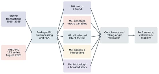
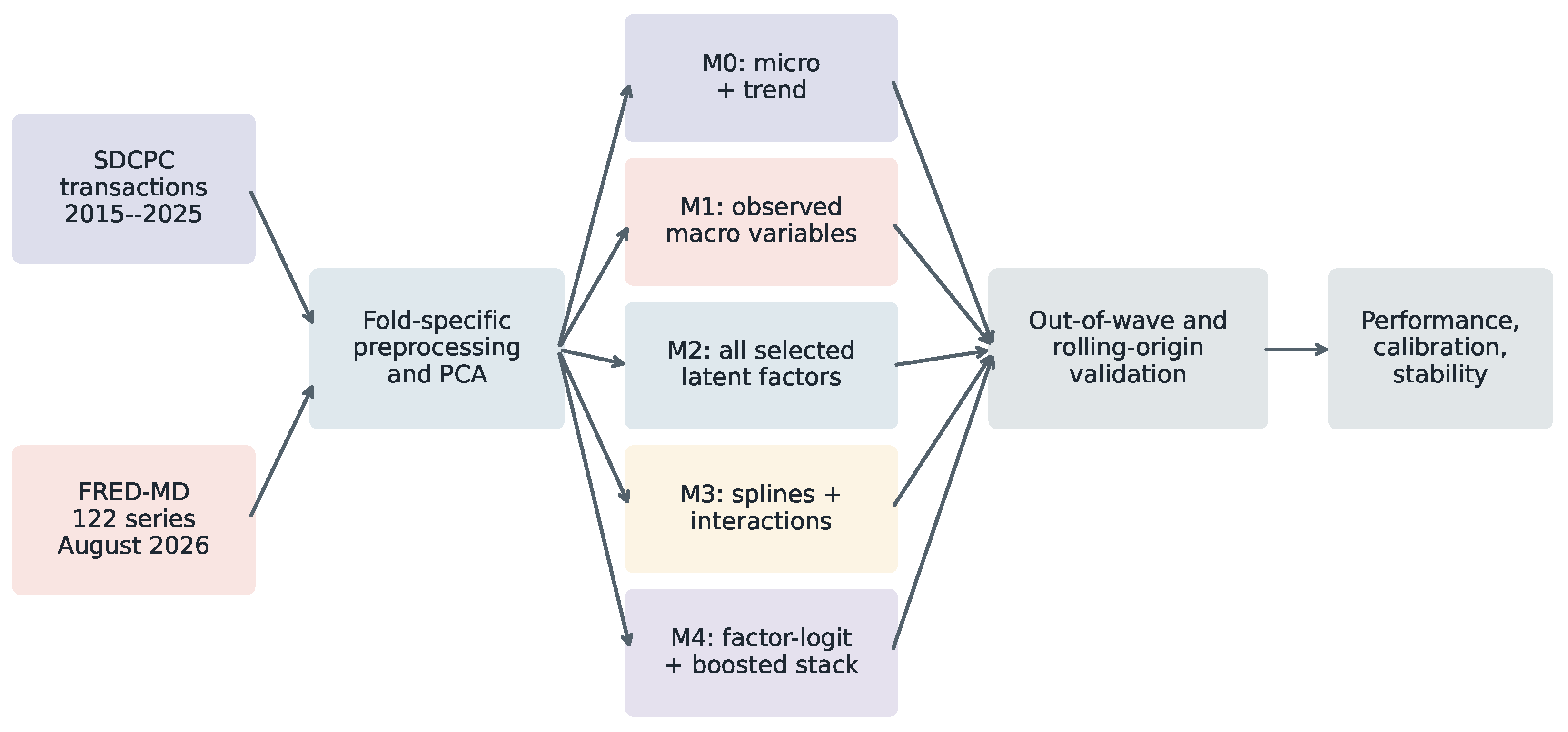
Figure 1 summarizes the complete workflow. The empirical and macroeconomic sources enter a fold-specific preprocessing stage before the architectures branch. Validation then reunites them under common metrics, calibration, comparison, stability, interpretation, and robustness procedures. This ordering prevents preprocessing choices from being treated as neutral steps outside the model.
Figure 1.
Leakage-controlled model-development and validation architecture.
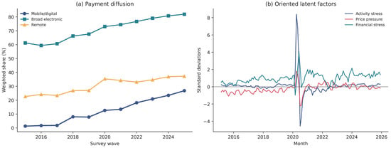
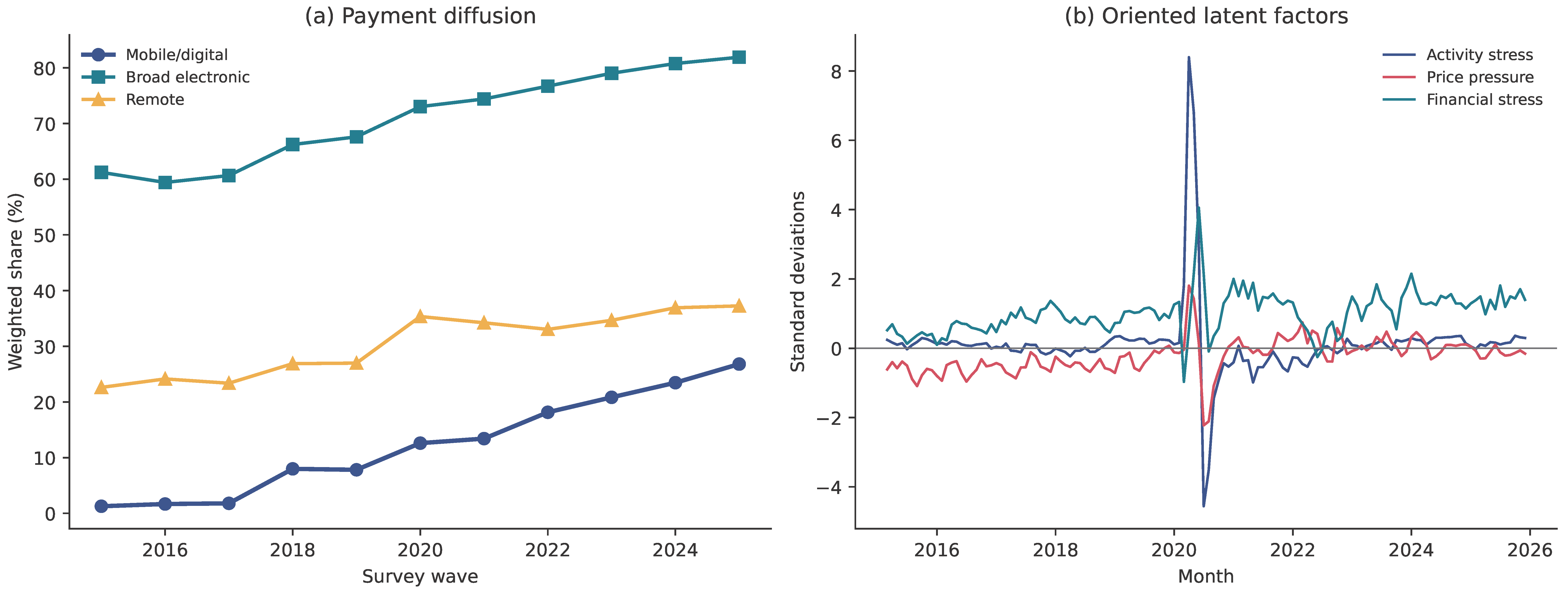
Figure 2 shows strong diffusion. The weighted mobile/digital share increases from 7.99% in 2018 to 26.81% in 2025. Broad electronic use rises from about 66% to 82%, while remote transactions rise from about 27% to 37%. The longer pre-2018 mobile series is shown for context but is not used as the primary comparable outcome because detailed mobile-method reporting is less stable. The factor panel shows why a single direct macro indicator is restrictive. Activity stress peaks during the pandemic, price pressure follows a different path, and financial stress has distinct episodes.
Figure 2.
Payment diffusion and oriented latent macroeconomic factors. Mobile/digital use before 2018 has a narrower measurement basis.
The secular increase creates a demanding validation problem. The positive-class share differs sharply between early and late folds, so a model must transport both rankings and probability levels. Transaction composition also changes: remote payments become more common and are strongly associated with mobile authorization. A model that ignores diffusion will underpredict later waves; a model that uses the wave label too aggressively can interpolate historical time but fail prospectively.
4.2. Econometric State-Dependence Models
Table 1 reports the weighted baseline. The composite-stress coefficient is −0.0064 with a wave-clustered standard error of 0.0057. Its restricted wild-cluster bootstrap p-value is 0.344. The stress–low-income interaction is positive (0.0076) but also imprecise (wild ). Remote status has a much larger association than either macro term. The baseline, therefore, supplies limited evidence that short-run macroeconomic state dependence is a stable component of mobile use after diffusion and transaction context are included.
Table 1.
Weighted mobile-payment state-dependence model, 2018–2025.
The distinction between asymptotic and few-cluster inference is material. For strict mobile instrument codes, the asymptotic cluster test suggests a positive stress coefficient, but the wild bootstrap does not reject (). The quadratic diffusion specification yields a more negative state coefficient, −0.0167, with wild . We investigated whether this change was due to mechanical collinearity. At the wave level, macro stress correlates 0.387 with centered linear trend and 0.367 with centered trend squared; after centering, the two trend terms are orthogonal. The variance-inflation factors are 1.21, 1.19, and 1.40 for linear trend, quadratic trend, and macro stress. Thus, the coefficient movement is not explained by severe multicollinearity. It instead reflects functional-form dependence when only eight annual macro states identify both diffusion and state effects. The quadratic result is, therefore, a sensitivity bound, not a retrospectively selected preferred estimate. Appendix E reports the full coefficient and diagnostic tables.
The multinomial model associates a one-standard-deviation stress increase with a 1.30-point decrease in mobile/digital probability and increases of 0.34 points for card, 0.39 points for account electronic, and 0.57 points for cash/paper. These marginal effects sum to approximately zero. They suggest reallocation rather than a uniform retreat from electronic instruments, but their regularized descriptive status and the few aggregate states preclude a structural interpretation.
4.3. Model Architecture Comparison
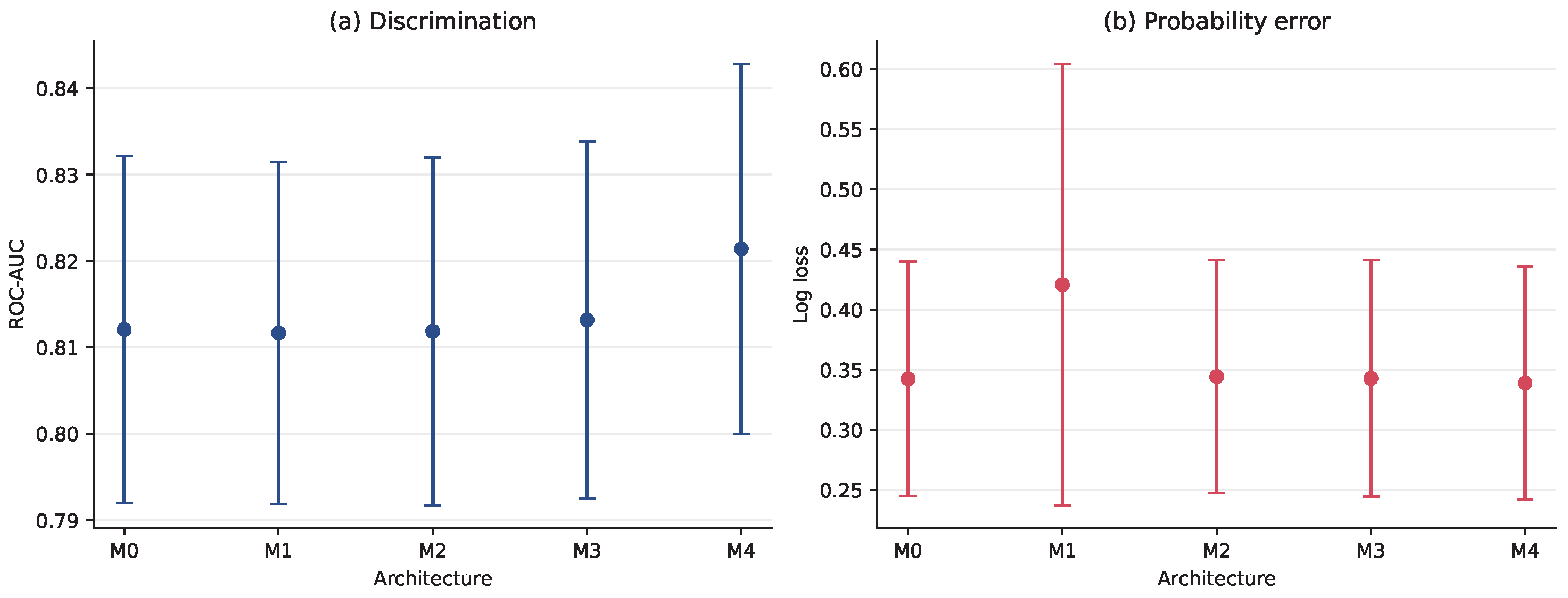
Table 2 contains the primary leave-one-wave-out results. M0 is already strong: log loss 0.3423, Brier score 0.1053, AUC 0.8121, and precision–recall AUC 0.4533. M1 leaves ranking essentially unchanged (AUC 0.8116) but worsens log loss to 0.4206 and Brier score to 0.1339. Direct macro indicators, therefore, change the probability scale without adding useful cross-wave ranking. Their coefficients extrapolate poorly when a test wave has an unusual combination of rates, inflation, and volatility.
Table 2.
Leave-one-wave-out predictive performance, 2018–2025.
M2 demonstrates the benefit and limit of latent compression. Its log loss of 0.3442 is close to M0 and far better than M1, showing that factors regularize direct macro information. Yet AUC 0.8118 is marginally below M0, and the Brier score is slightly higher. The macro panel contains coherent state information, but most of the signal relevant to transaction-level mobile use is already captured by micro variables and trend.
M3 raises AUC to 0.8131, a difference of only 0.0011 relative to M0. Its log loss is 0.3426, essentially unchanged. Spline flexibility consequently refines rankings but does not deliver a meaningful reduction in probability error. M4 provides the largest gain: AUC 0.8214, precision–recall AUC 0.4693, and log loss 0.3389. The hybrid uses the factor-logit score as a structured starting point and applies nonlinear corrections rather than asking trees to rediscover the entire signal.
Paired bootstrap comparisons in Table 3 clarify magnitude and uncertainty. The M4 AUC difference is 0.0093 with interval 0.0067 to 0.0120; every held-out wave favors M4 on AUC, yielding an exact two-sided sign-test . M3’s interval is also positive but economically small. M1 and M2 do not improve AUC. An AUC difference of 0.0093 means that M4 correctly orders roughly 9.3 additional randomly paired mobile/non-mobile transactions per 1000 pairs. For log loss, M4 improves by 0.0034 on average and wins in seven of eight waves (sign-test ), while its Brier improvement is less decisive. The gain is, therefore, consistent in ranking but modest in practical size and estimated from only eight paired differences.
Table 3.
Paired wave-bootstrap AUC differences relative to M0.
Equal weighting gives every macroeconomic state the same influence, which is appropriate for transport but gives the small and atypical 2020 wave the same weight as 2025. Weighting fold metrics by test-wave transaction counts leaves the conclusion nearly unchanged: M0 and M4 have AUC 0.8046 and 0.8137, respectively, and log loss 0.3772 and 0.3732. Appendix C reports both aggregation rules and every M4–M0 fold difference.
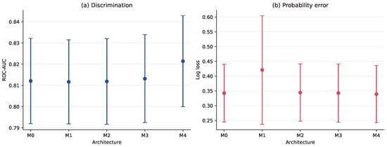
Figure 3 summarizes the mean discrimination and probability error of the five architectures across held-out waves.
Figure 3.
Mean leave-one-wave-out performance with one standard deviation across waves. Blue denotes ROC-AUC in panel (a), and red denotes log loss in panel (b); lower log loss is better.
4.4. Calibration and Temporal Generalization
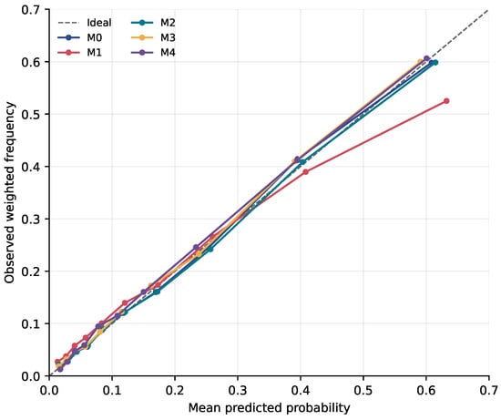
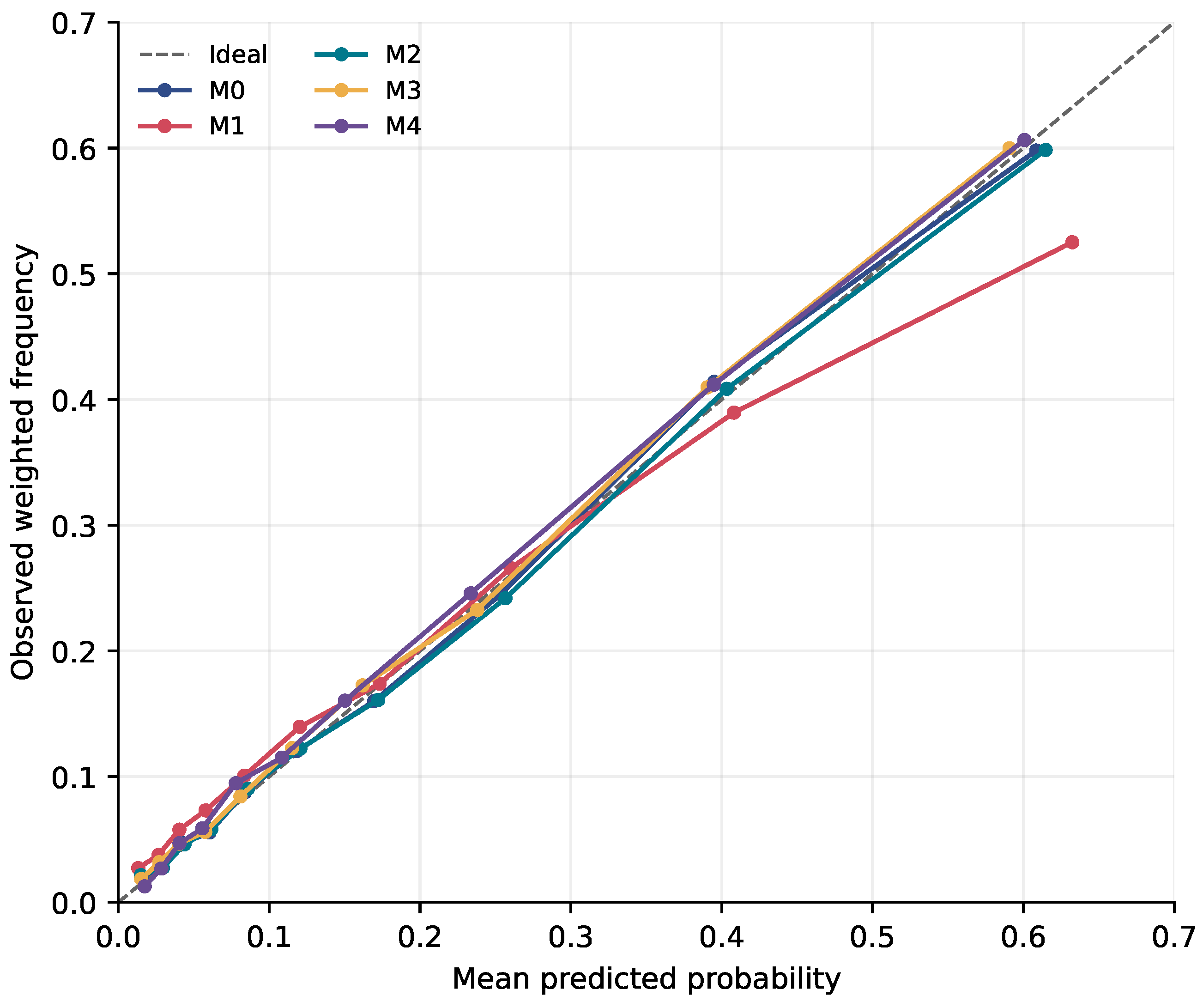
Figure 4 shows that M0, M2, M3, and M4 track the diagonal closely through most of the probability range. Their pooled calibration slopes are 0.985, 0.973, 0.988, and 0.991, respectively. M1 has intercept and slope 0.761, consistent with probabilities that are too dispersed and shifted when transported across waves. Latent compression, therefore, has a clear calibration advantage over direct macro indicators even though it does not beat the micro benchmark.
Figure 4.
Weighted out-of-wave calibration by predicted-probability decile.
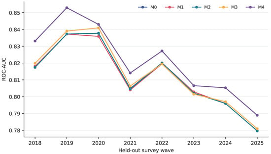
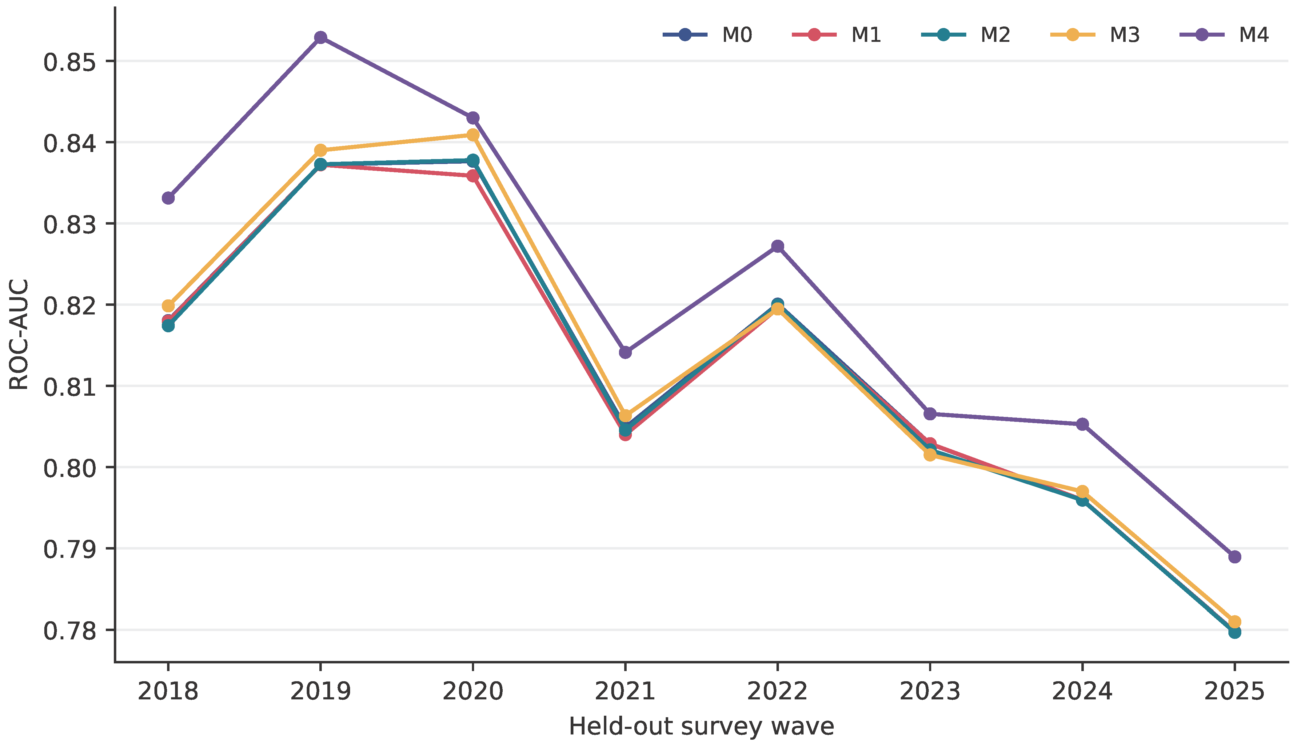
Performance varies temporally (Figure 5). All architectures reach their highest AUC near 2019–2020 and decline toward 2025. The parallel paths imply that later-wave difficulty is not resolved by macro variables or nonlinear flexibility. M4 improves AUC in every wave, but the separation remains approximately one percentage point rather than expanding in the later states.
Figure 5.
ROC-AUC by held-out survey wave. The dark-blue M0 trajectory is partially obscured where it overlaps with other model trajectories.
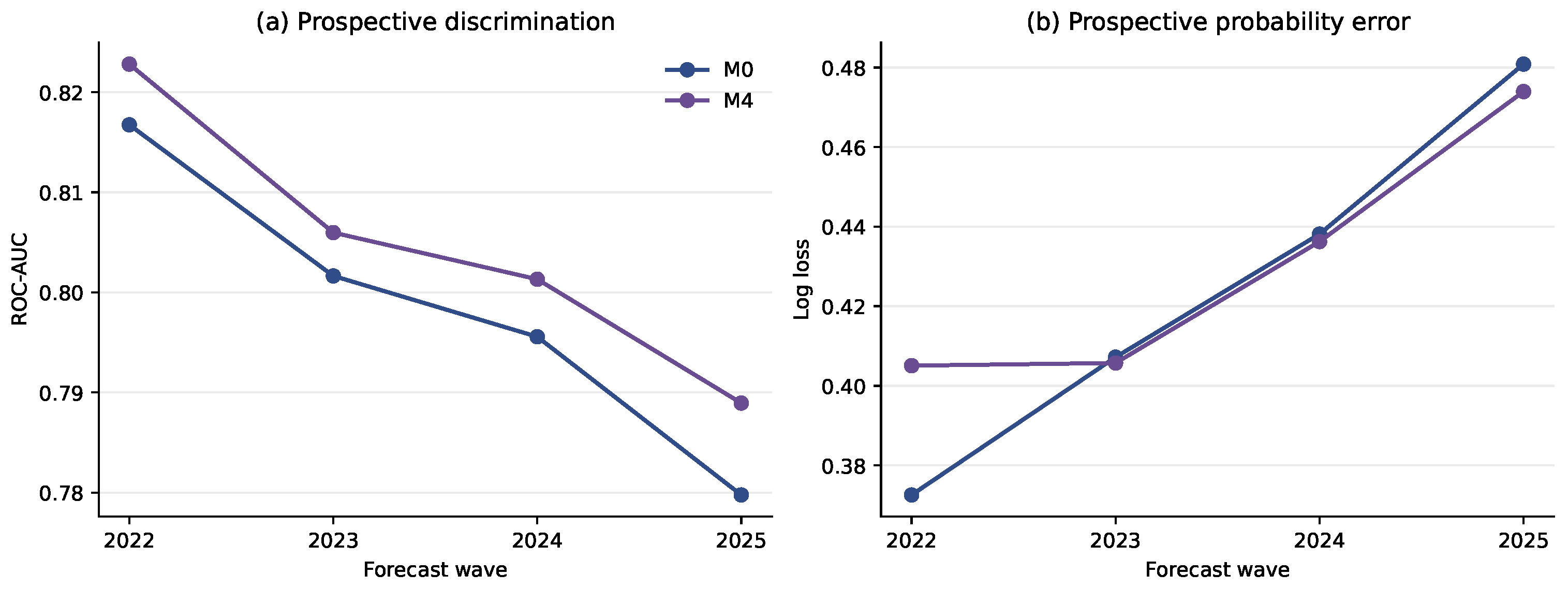
Rolling-origin validation makes the trade-off sharper (Figure 6). M0 averages AUC 0.7984 and log loss 0.4247 for 2022–2025. M4 raises AUC to 0.8048 but worsens log loss to 0.4302. The aggregate loss difference is driven by 2022: M4 improves that wave’s AUC from 0.8167 to 0.8228 but worsens log loss from 0.3726 to 0.4051, consistent with improved ordering but probabilities that are too extreme under the new state. M4 improves log loss in 2023–2025, including 0.4739 versus 0.4808 in 2025, yet not enough to offset 2022. M1 and M2 still have higher mean log loss. This fold-level pattern prevents selection of M4 solely from its retrospective leave-one-wave-out advantage.
Figure 6.
Rolling-origin performance for M0 and M4 by forecast wave. M4’s ranking advantage need not imply better probability calibration.
4.5. Interpretability, Stability, and Computational Complexity
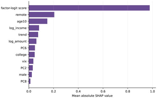
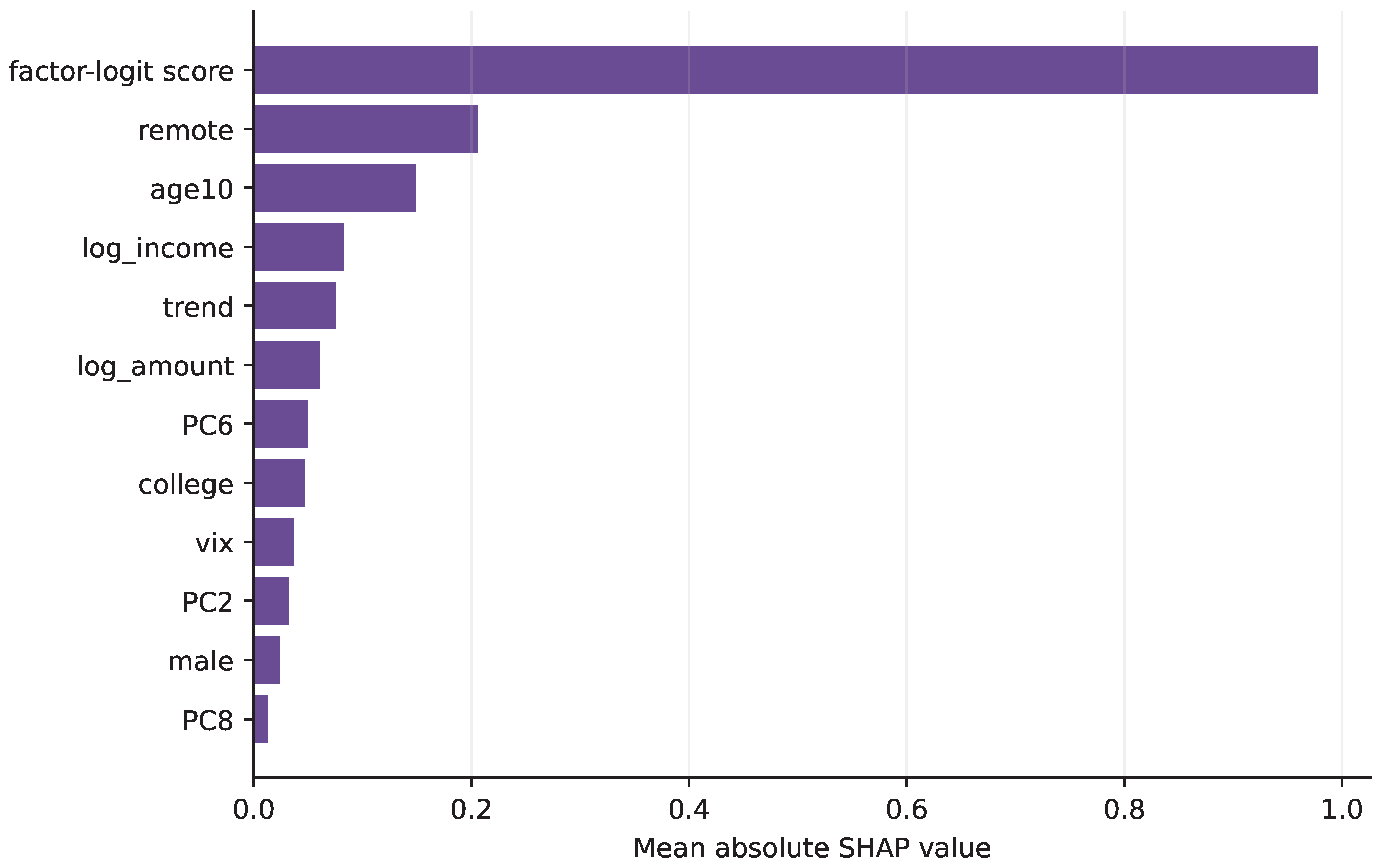
Figure 7 decomposes the full-sample hybrid. The factor-logit score is the dominant second-stage input, with a mean absolute SHAP value of 0.977. Remote status (0.206), age (0.149), log income (0.083), trend (0.075), and log amount (0.061) follow. The first explicit macro entries are PC6 (0.049) and VIX (0.037). This ordering supports the hybrid design: boosting mostly preserves the structured econometric score and adds selective corrections.
Figure 7.
Mean absolute SHAP values for the fitted M4 second stage. The factor-logit score aggregates M2’s micro, trend, and latent-factor information.
The stack complicates attribution of importance. A macro factor can influence the first-stage score even when its separate second-stage SHAP value is small. Consequently, the figure describes how M4 corrects M2; it is not a complete decomposition of structural economic influence. Remote status remains important both inside the base score and as a nonlinear correction. Its prominence is consistent with mobile payment as an interface tied closely to the transaction channel.
Stability also favors parsimony. The mean pairwise Spearman correlation of feature rankings across folds is 0.935 for M0, compared with 0.772 for M1, 0.766 for M2, 0.709 for M3, and 0.782 for M4. Additional features create more ways for importance to be redistributed across correlated predictors. M4 is more stable than M3 but less stable than M0.
Computational cost rises faster than predictive gain. Mean fitting time increases from 0.33 s for M0 to 0.94 for M2, 3.40 for M3, and 7.32 for M4. M4 is, therefore, about 22.4 times slower in relative terms, but the absolute difference is only about seven seconds per outer fold in this fixed, moderately sized exercise. It is not an operational barrier for a one-off fit. It becomes relevant when nested estimation is repeated across eight folds, many tuning grids, refreshed vintages, or governed deployment pipelines; prediction-time latency was not benchmarked and is not inferred from these training times. The model choice, therefore, depends on the loss attached to a one-point AUC difference, the need for calibrated probabilities, and the governance value of a transparent specification.
4.6. Robustness and Sensitivity
Robustness evidence does not support a single invariant macroeconomic coefficient. The baseline composite association is negative and imprecise. Unweighted and pandemic-excluded estimates remain negative and imprecise. In-person transactions and the strict code outcome change the sign. Separate activity, price, and financial factors also fail to provide stable wild-bootstrap rejection. The quadratic trend is the exception, producing a larger negative coefficient, but the low VIFs show that this is functional-form uncertainty rather than severe collinearity. Figure A3 and Table A14 and Table A15 report these estimates and diagnostics together.
The predictive sensitivity analyses re-estimate all five architectures rather than changing only the econometric outcome. For the strict code outcome (weighted prevalence 1.51%), M0 and M4 have AUC 0.7568 and 0.7546, so the primary M4 AUC gain does not replicate; M4 nevertheless raises precision–recall AUC from 0.0446 to 0.0537 and slightly lowers log loss from 0.0717 to 0.0707. Under strict rolling-origin validation, neither model dominates. For in-person transactions, M4 raises AUC from 0.6737 to 0.6919, although both models are much weaker than in the full sample. Excluding 2020–2021 leaves the primary ranking intact (AUC 0.8090 versus 0.8175). These results narrow the claim: M4’s benefit depends on how device-mediated use is measured and is strongest for ranking the broader authorization outcome, not for every definition of mobile payment. Appendix E reports the full table and figure.
5. Discussion
The evidence changes how temporal stability in digital payment use should be described. Mobile use rises through a pandemic, inflation, monetary tightening, and market volatility, but that coexistence does not identify resilience to those shocks. Much of the stable predictive structure comes from transaction channel, age, income, amount, and diffusion. Once these are represented, the macroeconomic panel adds limited incremental transaction-level predictive information. This finding does not imply that aggregate conditions are unimportant for welfare, access, merchant investment, or payment-system stability; those outcomes are not the estimand.
The comparison between M1 and M2 is particularly informative. Direct observable indicators are economically legible, but their cross-wave combinations are difficult to transport. They preserve AUC while damaging log loss and calibration. Principal components compress the same broad state space and largely eliminate that damage. Latent factors, therefore, contribute as a stabilization device even when they do not improve discrimination beyond M0. This is a modeling contribution distinct from finding a significant factor coefficient.
The limited difference between M0 and M3 suggests that smooth nonlinearities and two targeted interactions do not transform the problem. A regularized linear predictor already captures most of the persistent ordering. M4 obtains a consistent AUC improvement for the primary outcome by treating M2 as a structured score and learning residual nonlinearities. Yet the gain is less than one AUC point, balanced accuracy barely changes, feature rankings become less stable, rolling-origin log loss worsens, and the strict-code AUC does not improve. There is no metric-free or outcome-definition-free winner.
These results are consistent with earlier payment-choice studies while extending them in a different direction. The importance of amount and checkout context accords with transaction-level evidence in Klee (2008); persistent demographic and adoption structure accords with Koulayev et al. (2016) and the separation between a mobile interface and its funding rail follows the classification problem emphasized by Trütsch (2016). The role of remote status is also consistent with pandemic-era changes documented by Greene et al. (2021); Greene and Stavins (2023). Our contribution is not another coefficient for one determinant. It is evidence that these established micro and transaction signals transport more reliably across U.S. waves than raw observable macro indicators, while factor compression protects calibration. The nonlinear inflation regimes studied by Dinh (2025) further caution against assuming a universal linear macro channel, but their cross-country digital-inclusion outcome is not directly comparable to transaction-level use.
For applications that require rank ordering—for example, targeting usability research toward transactions least likely to use a mobile interface—M4 may be justified. For probability-sensitive decisions, reporting, scenario analysis, or environments with limited computational governance, M0 or M2 may be preferable. M0 has the strongest ranking stability and the best rolling-origin log loss. M2 sacrifices almost no performance while providing an explicit representation of macroeconomic state. The choice between them depends on whether macroeconomic scenario sensitivity is itself an output requirement.
The econometric and predictive findings are compatible. The baseline state coefficient is negative but imprecise under preferred few-cluster inference. Factors also add little transaction-level predictive value. Neither result establishes the absence of macroeconomic influence. The quadratic trend illustrates identification uncertainty, and M4’s modest gain shows that some state information can contribute through nonlinear combinations. The appropriate conclusion is limited robust incremental value, not a precisely estimated zero effect.
Remote status deserves substantive attention. It is the strongest direct predictor in the econometric model and the most important correction after the hybrid base score. Mobile authorization is embedded in an ecosystem of devices, merchant interfaces, authentication processes, and underlying rails. Within this U.S. sample, where and how a purchase is made contains more predictive signal than any single national macro indicator. This is not evidence that expanding merchant acceptance or changing infrastructure would causally raise use. It instead indicates that providers evaluating prediction systems should represent transaction channel before adding a large macro block, while regulators should continue to assess operational resilience, interoperability, consumer protection, and access with evidence designed for those distinct outcomes.
Income differences require similarly careful interpretation. Low income is relevant to levels of payment access and funding choice, but the stress interaction is unstable. A nonsignificant interaction is not evidence that vulnerable consumers face identical constraints. It means that eight national survey waves do not deliver a precise differential macro response after controls. Policy analysis should not replace persistent access gaps with an unsupported claim of cyclical homogeneity.
Several limitations bound the findings. First, public-use file structures and questions change across waves. The 2018–2025 restriction and strict-code robustness improve comparability, but the broader authorization outcome cannot be proven perfectly measurement-invariant, and its 1.51% strict-code counterpart describes a narrower construct. Second, diary observations are clustered within respondents as well as waves. The prediction design blocks waves, while the inferential focus clusters at the level of macro exposure; richer multiway dependence would require more aggregate clusters. Third, eight annual waves provide only eight comparable macro states, and the small, atypical 2020 sample makes uncertainty across states more important than the nominal transaction count. Equal- and volume-weighted results agree, but neither creates additional state variation. Fourth, most annual diary activity occurs around October, limiting within-year macro variation. Fifth, the August 2026 FRED-MD vintage contains retrospective revisions and does not recreate the release set available to a forecaster in each year. Sixth, factor labels are sign-normalized statistical summaries rather than rotated or identified shocks. Seventh, the hybrid settings are fixed and deliberately moderate; extensive tuning might improve M4 but would increase selection risk and computational cost. Eighth, SHAP values are conditional on the fitted stack and correlated inputs. Finally, the U.S. payment environment may not generalize to economies with different account access, mobile-money infrastructure, inflation histories, or regulatory institutions.
Future extensions should add aggregate states before adding many algorithms. More annual waves would improve separation of diffusion and macro dependence. Regionally identified diaries could exploit local labor-market and financial variation. Respondent panels could model switching and habit formation. Merchant attributes, fees, outages, fraud, and platform availability would connect economic resilience to operational resilience. Methodologically, distribution-shift calibration, conformal prediction by wave, and hierarchical dynamic models could provide uncertainty estimates for new states. These extensions would address information limits visible here rather than treating algorithmic complexity as a substitute for design.
6. Conclusions
This study compares five progressively richer architectures for modeling transaction-level digital payment use across changing macroeconomic states. The design links 182,409 U.S. payment records to 122 FRED-MD indicators, reconstructs preprocessing within each held-out wave, and evaluates both retrospective leave-one-wave-out transport and pseudo-prospective rolling-origin prediction.
The central result is a bounded and outcome-dependent return to complexity. A microeconomic regularized logit with structural diffusion attains AUC 0.8121. Direct macro indicators worsen probability performance. Latent factors stabilize the macro information but do not outperform the benchmark. Spline interactions add negligible improvement. A hybrid factor-logit/boosting stack raises primary-outcome AUC to 0.8214 and improves leave-one-wave-out log loss, but has less stable feature rankings, does not improve rolling-origin log loss, and does not improve AUC for the strict instrument-code outcome.
The financial-economics contribution is a decision rule for model complexity rather than a universal winning algorithm. Macroeconomic information should enter as a tested incremental layer above a strong transaction-level benchmark. A simpler M0 or M2 specification is defensible for calibrated probabilities, scenario reporting, transparent governance, or frequent updating. M4 is defensible when rank ordering has measurable value and a gain of roughly nine additional correctly ordered pairs per 1000 justifies nested fitting. Latent compression is preferable to a direct state block when macroeconomic representation is required without sacrificing calibration.
Econometric results provide limited robust evidence of a short-run composite-stress association after diffusion and transaction context are represented. A quadratic trend produces a larger negative estimate despite low VIFs, underscoring functional-form uncertainty when only eight waves separate diffusion from state dependence. The appropriate conclusion is limited incremental predictive and associational evidence in this U.S. sample—not that payment systems are structurally resilient, that macroeconomic conditions are irrelevant, or that any channel is causal.
Author Contributions
Conceptualization, A.F.O.-M., O.J.-B. and S.L.-E.; methodology, A.F.O.-M., O.J.-B. and S.L.-E.; software, formal analysis, data curation and visualization, A.F.O.-M.; validation, A.F.O.-M. and S.L.-E.; investigation, A.F.O.-M., O.J.-B. and S.L.-E.; writing—original draft preparation, A.F.O.-M.; writing—review and editing, A.F.O.-M., O.J.-B. and S.L.-E.; supervision, O.J.-B. and S.L.-E.; project administration, O.J.-B. All authors have read and agreed to the published version of the manuscript.
Funding
This research received no external funding.
Institutional Review Board Statement
Not applicable. The analysis uses anonymized public-use secondary data.
Informed Consent Statement
Not applicable.
Data Availability Statement
The SDCPC public-use files are available from the Federal Reserve Bank of Atlanta. FRED-MD is available from the Federal Reserve Bank of St. Louis.
Acknowledgments
During preparation of this manuscript, the authors used OpenAI ChatGPT (GPT-5, accessed on September 2026) for language editing. The authors reviewed and take full responsibility for the content.
Conflicts of Interest
The authors declare no conflicts of interest.
Appendix A. Data Harmonization and Payment Taxonomy
Figure A1 and Table A1 consolidate the sample construction from raw transaction candidates to the two analysis samples. Predictor imputation in the predictive models occurs inside each training fold; it, therefore, does not reduce the 146,507-row predictive sample. Complete-case deletion is used only for the econometric model.
Figure A1.
Sample-construction flow. Percentages above arrows are retention rates from the preceding stage.

Table A1.
Consolidated analytic sample construction.
Table A2 shows how combined 2015–2016 files and separate 2017–2025 files pass the same payment and valid-instrument filters. In 2021 and 2022, the payment flag and instrument validity do not nest perfectly; the final column is their intersection, not either marginal count.
Table A3 reports the annual sample and weighted shares. The primary mobile definition uses detailed authorization information from 2018 onward; the strict outcome uses only instrument codes 10 and 12. Broad electronic use contains card, account-electronic, and official mobile instruments. Remote indicates that the transaction was not in person.
Table A2.
Wave-specific source layout and harmonization counts.
Table A3.
Annual sample inventory and weighted payment shares.
The mutually exclusive taxonomy applies the following precedence: mobile/digital, cash/paper, card, account electronic, and residual other. This ordering avoids assigning a mobile-wallet card transaction to the card class before recognizing its mobile interface. Card and account funding outcomes remain available separately. Table A4 reports the regularized multinomial stress marginal effects.
Table A4.
Multinomial average marginal effects of composite macroeconomic stress.
Appendix B. Factor Construction and Diagnostics
The August 2026 FRED-MD file contains 126 named columns plus a date field; four columns are removed because a valid transformation code or sufficient coverage is unavailable. Transformations follow the supplied codes. For the full retrospective basis, median imputation and standardization are estimated over 1962–2025. Figure A2 shows the ICp2 minimum at eight factors and the associated variance decomposition. The first component explains about 19% of standardized-panel variation, and the first eight explain about 52%.
Figure A2.
Factor-number selection and explained variance. In panel (a), the blue line shows the ICp2 criterion and the red dashed line marks the selected eight-factor solution. In panel (b), teal bars show the variance explained by each component and the red line shows cumulative explained variance.
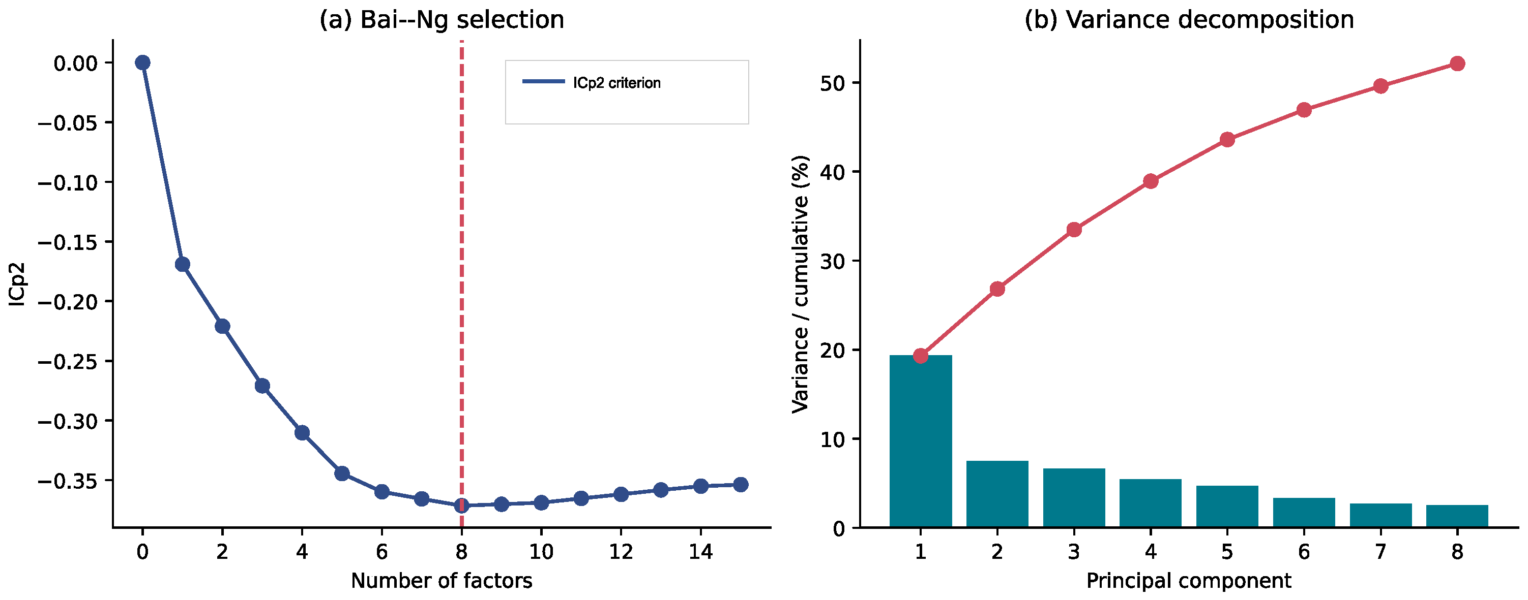
Table A5 shows fold-specific factor selection. Early cutoffs yield six factors; the criterion selects eight once the pre-wave macro history extends through 2020. All test observations are projected using the basis estimated before their diary window.
Table A5.
Fold-specific Bai–Ng selection and sample sizes.
Table A6 documents the descriptive orientations. PC1, PC3, and PC7 are selected by their absolute correlations with the three anchors over 1985–2025; only their signs are normalized. No orthogonal or oblique rotation is applied, and the labels do not identify structural shocks. The predictive models use every factor selected within a fold, including components without an economic label.
Table A6.
Sign normalization and descriptive interpretation of selected principal components.
Appendix C. Extended Model Diagnostics
Table A7 records calibration intercepts and slopes. The deterioration of M1 occurs mainly in the probability scale rather than ranking. M2’s latent compression restores a slope near one. M4 is closest to the ideal pooled slope, although its rolling-origin log loss remains worse than M0.
Table A7.
Pooled leave-one-wave-out calibration parameters.
Table A8 summarizes importance stability. Rank correlation is computed for every pair of held-out waves after taking the union of available features and assigning zero to absent fold-specific components. The comparison is descriptive because coefficient magnitude and tree gain are different importance scales; correlations are only compared within architecture across time.
Table A8.
Feature-importance rank stability across held-out waves.
Table A9.
Leading mean absolute SHAP values for the full hybrid second stage.
Table A10 compares equal-wave and transaction-volume weighting. The M4 advantage over M0 is similar under both rules, showing that the primary conclusion is not driven by the small 2020 wave.
Table A10.
Sensitivity of predictive summaries to fold-aggregation weights.
Table A11.
Fold-level M4 differences relative to M0.
Appendix D. Rolling-Origin Validation
Table A12 evaluates 2022–2025 with training restricted to earlier waves. Discrimination and probability accuracy point to different selections. M4 has the highest AUC and precision–recall AUC, whereas M0 has the lowest log loss and Brier score. M3 achieves the highest balanced accuracy. The result reinforces a decision-specific rather than universal architecture ranking.
Table A12.
Rolling-origin predictive performance, 2022–2025.
Table A13 displays the M0–M4 comparison in each forecast wave.
Table A13.
Fold-level rolling-origin comparison of M0 and M4.
Appendix E. Robustness and Sensitivity Analysis
Figure A3 and Table A14 compare macroeconomic-state coefficients. Confidence intervals use wave-clustered standard errors; inference in the table uses the restricted wild-cluster bootstrap. The quadratic trend is the only specification that rejects at 5%. Its difference from the baseline is interpreted as trend-model uncertainty, not as a preferred retrospective result.
Figure A3.
Macroeconomic-state coefficients across robustness specifications. Blue denotes estimates with wild-cluster , and red denotes wild-cluster .
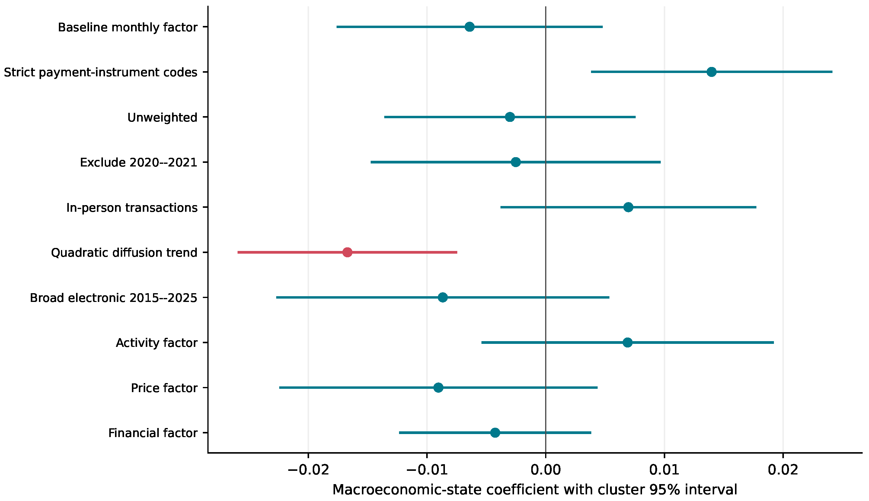
Table A14.
Robustness of macroeconomic-state estimates.
Table A15.
Wave-level trend–macroeconomic-state diagnostics.
Figure A4 and Table A16 report predictive robustness in which the complete M0–M4 sequence is re-estimated. The strict instrument-code outcome is rare; precision–recall AUC and log loss are consequently important complements to ROC-AUC. The figure focuses on M4 relative to M0.
Figure A4.
Predictive robustness of M4 relative to M0. Positive AUC favors M4; negative log loss favors M4.
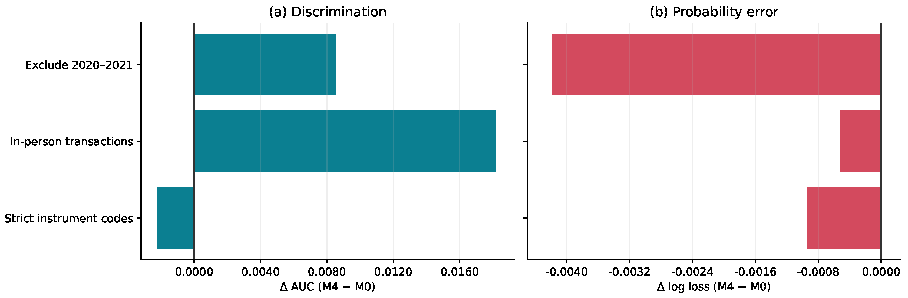
Table A16.
Predictive robustness under alternative outcomes, samples, and validation designs.
References
- Arlot, S., & Celisse, A. (2010). A survey of cross-validation procedures for model selection. Statistics Surveys, 4, 40–79. [Google Scholar] [CrossRef] [Scilit]
- Bai, J., & Ng, S. (2002). Determining the number of factors in approximate factor models. Econometrica, 70(1), 191–221. [Google Scholar] [CrossRef] [Scilit]
- Breiman, L. (2001). Statistical modeling: The two cultures. Statistical Science, 16(3), 199–231. [Google Scholar] [CrossRef] [Scilit]
- Cameron, A. C., Gelbach, J. B., & Miller, D. L. (2008). Bootstrap-based improvements for inference with clustered errors. Review of Economics and Statistics, 90(3), 414–427. [Google Scholar] [CrossRef] [Scilit]
- Chen, T., & Guestrin, C. (2016). XGBoost: A scalable tree boosting system. In Proceedings of the 22nd ACM sigkdd international conference on knowledge discovery and data mining (pp. 785–794). Association for Computing Machinery. [Google Scholar] [CrossRef] [Scilit]
- Cohen, R., Shy, O., & Stavins, J. (2022). Payments evolution from paper to electronic payments by merchant type (Tech. Rep. No. 22-6). Federal Reserve Bank of Boston. [Google Scholar] [CrossRef]
- Dinh, L. Q. (2025). The optimal inflation threshold in digital financial inclusion: A key to sustainable development. SN Business & Economics, 5(5), 40. [Google Scholar] [CrossRef] [Scilit]
- Federal Reserve Bank of Atlanta. (2025). Survey and diary of consumer payment choice: 2025 codebook. Available online: https://www.atlantafed.org/banking-and-payments/consumer-payments/survey-and-diary-of-consumer-payment-choice (accessed on 30 October 2026).
- Federal Reserve Bank of St. Louis. (2026). FRED-MD monthly database. Available online: https://www.stlouisfed.org/research/economists/mccracken/fred-databases (accessed on 30 October 2026).
- Felt, M.-H., Laferrière, A., & Leduc, S. (2023). The distributional effects of payment choice. Journal of Banking & Finance, 151, 106968. [Google Scholar] [CrossRef] [Scilit]
- Friedman, J. H. (2001). Greedy function approximation: A gradient boosting machine. The Annals of Statistics, 29(5), 1189–1232. [Google Scholar] [CrossRef] [Scilit]
- Goldfarb, A., & Tucker, C. (2019). Digital economics. Journal of Economic Literature, 57(1), 3–43. [Google Scholar] [CrossRef] [Scilit]
- Gomber, P., Koch, J. A., & Siering, M. (2017). Digital finance and FinTech: Current research and future research Directions. Journal of Business Economics, 87, 537–580. [Google Scholar] [CrossRef] [Scilit]
- Greene, C., Merry, E., & Stavins, J. (2021). Has COVID changed consumer payment behavior? (Tech. Rep. No. 21-12). Federal Reserve Bank of Boston. [Google Scholar] [CrossRef]
- Greene, C., & Stavins, J. (2023). Changes in U.S. payment behaviour during COVID-19: Differences by income and demographics. Journal of Payments Strategy & Systems, 17, 1–18. [Google Scholar] [CrossRef] [Scilit]
- Greene, C., & Stavins, J. (2024). Credit card behavior and consumer finances. Journal of Financial Services Research, 65, 1–31. [Google Scholar] [CrossRef] [Scilit]
- Hand, D. J. (2009). Measuring classifier performance: A coherent alternative to the area under the ROC Curve. Machine Learning, 77, 103–123. [Google Scholar] [CrossRef] [Scilit]
- Klee, E. (2008). How people pay: Evidence from grocery store data. Journal of Monetary Economics, 55(3), 526–541. [Google Scholar] [CrossRef] [Scilit]
- Koulayev, S., Rysman, M., Schuh, S., & Stavins, J. (2016). Explaining adoption and use of payment instruments by U.S. consumers. RAND Journal of Economics, 47(2), 293–325. [Google Scholar] [CrossRef] [Scilit]
- Lundberg, S. M., & Lee, S.-I. (2017). A unified approach to interpreting model predictions. In Advances in neural information processing systems (Vol. 30). Neural Information Processing Systems Foundation. [Google Scholar]
- MacKinnon, J. G., & Webb, M. D. (2017). Wild bootstrap inference for wildly different cluster sizes. Journal of Applied Econometrics, 32(2), 233–254. [Google Scholar] [CrossRef] [Scilit]
- McCracken, M. W., & Ng, S. (2016). FRED-MD: A monthly database for macroeconomic research. Journal of Business & Economic Statistics, 34(4), 574–589. [Google Scholar] [CrossRef] [Scilit]
- Roberts, D. R., Bahn, V., Ciuti, S., Boyce, M. S., Elith, J., Guillera-Arroita, G., Hauenstein, S., Lahoz-Monfort, J. J., Schröder, B., Thuiller, W., Warton, D. I., Wintle, B. A., Hartig, F., & Dormann, C. F. (2017). Cross-validation strategies for data with temporal, spatial, hierarchical, or phylogenetic structure. Ecography, 40(8), 913–929. [Google Scholar] [CrossRef] [Scilit]
- Schuh, S., & Stavins, J. (2010). Why are (some) consumers (finally) writing fewer checks? Journal of Banking & Finance, 34(8), 1745–1758. [Google Scholar] [CrossRef] [Scilit]
- Shy, O. (2020). Low-income consumers and payment choice. Research in Economics, 74(4), 292–300. [Google Scholar] [CrossRef] [Scilit]
- Stavins, J. (2018). Consumer preferences for payment methods: Role of discounts and surcharges. Journal of Banking & Finance, 94, 35–53. [Google Scholar] [CrossRef] [Scilit]
- Steyerberg, E. W., Vickers, A. J., Cook, N. R., Gerds, T., Gonen, M., Obuchowski, N., Pencina, M. J., & Kattan, M. W. (2010). Assessing the performance of prediction models: A framework for traditional and novel measures. Epidemiology, 21(1), 128–138. [Google Scholar] [CrossRef] [Scilit] [PubMed]
- Stock, J. H., & Watson, M. W. (2002). Forecasting using principal components from a large number of predictors. Journal of the American Statistical Association, 97(460), 1167–1179. [Google Scholar] [CrossRef] [Scilit]
- Train, K. E. (2009). Discrete choice methods with simulation (2nd ed.). Cambridge University Press. [Google Scholar] [CrossRef] [Scilit]
- Trütsch, T. (2016). The impact of mobile payment on payment choice. Financial Markets and Portfolio Management, 30, 299–336. [Google Scholar] [CrossRef] [Scilit]
- Van Calster, B., McLernon, D. J., van Smeden, M., Wynants, L., & Steyerberg, E. W. (2019). Calibration: The achilles heel of predictive analytics. BMC Medicine, 17, 230. [Google Scholar] [CrossRef] [Scilit] [PubMed]
- Yarkoni, T., & Westfall, J. (2017). Choosing prediction over explanation in psychology: Lessons from machine learning. Perspectives on Psychological Science, 12(6), 1100–1122. [Google Scholar] [CrossRef] [Scilit] [PubMed]

Disclaimer/Publisher’s Note: The statements, opinions and data contained in all publications are solely those of the individual author(s) and contributor(s) and not of MDPI and/or the editor(s). MDPI and/or the editor(s) disclaim responsibility for any injury to people or property resulting from any ideas, methods, instructions or products referred to in the content. |
© 2026 by the authors. Licensee MDPI, Basel, Switzerland. This article is an open access article distributed under the terms and conditions of the Creative Commons Attribution (CC BY) license.