Credit Expansion, Housing Cycles and Financial Stability: Cross-Country Evidence on Boom-and-Bust Dynamics, 1995 to 2025

Abstract

Whether credit expansion systematically drives house price booms, raises the probability of subsequent busts, and impairs bank balance sheets remains an open empirical question. Historical evidence and the financial cycle literature point in that direction, but few studies analyse the three links within a single framework or cover the corrections that followed the post-pandemic boom. This paper assembles an annual panel of 57 economies for 1995 to 2025 from the Bank for International Settlements residential property price series and the World Bank World Development Indicators, and identifies 37 real house price busts, defined as cumulative real declines of at least 15 percent from a local peak within six years. Country fixed effects regressions show that a one percentage point increase in the ratio of private credit to GDP raises real house price growth in the following year by 0.17 to 0.21 percentage points. Logistic models predict busts up to three years ahead with an area under the ROC curve of 0.79 to 0.84; the odds of a bust are 3.8 times higher after a credit boom and 2.4 times higher after a house price boom, and the bust rate reaches 30 percent when both booms coincide, compared to 5 percent otherwise. During busts, the ratio of non-performing loans rises by about one percentage point per year more than in other periods, with an additional effect of the preceding credit expansion. The results are robust across advanced, euro area and emerging economies, to the low interest rate period after 2008 and to alternative bust definitions, and they provide quantitative benchmarks for countercyclical macroprudential policy.

1. Introduction

Financial stability is rarely lost in a single moment. It erodes gradually, during years in which credit grows faster than income, collateral values rise faster than rents, and the perceived riskiness of lending falls precisely when exposure is accumulating. Housing markets are the arena in which this process is most visible because residential property is simultaneously the largest asset of households, the dominant form of collateral in bank lending and the sector most sensitive to the cost and availability of credit. The global financial crisis of 2007 to 2009, the peripheral euro area crisis that followed and the synchronised correction of real house prices in several advanced economies after the monetary tightening of 2022 all share this pattern of credit-fuelled expansion followed by abrupt revaluation.

The question of whether credit expansion causes housing booms, or merely accompanies them, is not new. von Mises (1912/1953) and Hayek (1931, 1933) argued that an expansion of bank credit not backed by prior saving lowers the market rate of interest below its natural level, distorts the intertemporal structure of production and generates malinvestment that must eventually be liquidated. Huerta de Soto (2006) extended this analysis to the institutional features of fractional reserve banking and, in a treatment that anticipated much of the post-2008 debate, emphasised the role of real estate as the preferred vehicle of malinvestment in modern economies. In parallel, and from a different methodological tradition, Minsky (1986) and Kindleberger and Aliber (2005) described financial fragility as an endogenous outcome of prolonged stability, while the empirical financial cycle literature associated with the Bank for International Settlements (Borio & Lowe, 2002; Drehmann et al., 2012; Borio, 2014) and the long-run historical work of Schularick and Taylor (2012) and Jordà et al. (2015, 2016) documented that credit booms, and especially mortgage credit booms, are the single most robust predictor of financial crises.

Despite this convergence between theoretical traditions and historical evidence, three empirical gaps remain. First, most cross-country studies of housing busts stop in 2010 or shortly after and therefore exclude the post-pandemic boom of 2020 to 2022 and the real price corrections that followed in Germany, Sweden, Canada, New Zealand, Finland, Austria and Luxembourg. Second, the literature tends to study either the price side of the cycle (what predicts a bust) or the balance sheet side (what happens to banks after a bust), but seldom both in the same framework with the same data. Third, few papers make explicit the connection between the empirical regularities and the mechanisms proposed by the Austrian theory of the cycle, which is arguably the oldest and most complete account of why credit expansion should systematically generate boom-and-bust dynamics in long-lived capital goods such as housing.

This paper addresses these gaps with a deliberately transparent empirical design based exclusively on official statistics. We construct an annual panel of 57 economies covering the period 1995 to 2025, combining the selected residential property price series compiled by the Bank for International Settlements (BIS) with the World Development Indicators (WDI) of the World Bank, which in turn draw on the International Monetary Fund and national statistical offices. Using a simple peak and trough algorithm, we identify 37 real house price busts during the sample period, each involving a cumulative real decline of at least 15 percent within six years of a local peak. We then ask three questions. Does credit expansion predict real house price growth one year ahead, once country heterogeneity and the macroeconomic environment are controlled for? Does the conjunction of a credit boom and a house price boom raise the probability that a bust begins within the next three years, and how well do such models discriminate between bust and non-bust years? And do busts, together with the credit expansion that preceded them, translate into a measurable deterioration of bank asset quality as captured by the ratio of non-performing loans?

Our contribution is threefold. Empirically, we provide updated cross-country estimates that include the 2022 to 2025 corrections and that report both cluster-robust and heteroskedasticity-consistent (HC3) standard errors, odds ratios with confidence intervals, and discrimination statistics (area under the ROC curve) that allow direct comparison with the early warning literature. Theoretically, we show that the pattern of results, namely the primacy of credit growth over other macroeconomic variables in predicting house price growth and busts, the amplification when credit and price booms coincide, and the lagged transmission of busts to bank balance sheets, is consistent with the sequence described by the Austrian theory of the credit cycle and complements the financial accelerator and leverage cycle explanations. From a policy perspective, we translate the estimates into quantitative benchmarks: a bust rate of 30 percent within three years when a credit boom and a house price boom coincide, compared to 5 percent otherwise, is the kind of number that a countercyclical capital buffer framework can act upon.

The remainder of the paper is organised as follows. Section 2 reviews the theoretical framework and the empirical literature and states the hypotheses. Section 3 describes the data sources, the identification of bust episodes, the variables, and the estimation strategy. Section 4 presents the results: the catalogue of episodes and descriptive statistics, bivariate tests, panel regressions for real house price growth, logistic models for bust prediction, regressions for the dynamics of non-performing loans, and robustness checks. Section 5 discusses the findings in light of the literature, examines unexpected results, and acknowledges limitations. Section 6 concludes with policy implications and directions for future research.

2. Theoretical Framework and Literature Review

2.1. The Austrian Theory of the Credit Cycle and the Housing Market

The Austrian theory of the business cycle, developed by von Mises (1912/1953) in the first edition of his monetary treatise of 1912 and refined by Hayek (1931, 1933), starts from a distinction between two sources of loanable funds. When banks lend out of genuine savings, the rate of interest coordinates the intertemporal plans of savers and investors and the structure of production adjusts to consumer time preferences. When banks instead expand credit through the creation of deposits, the market rate of interest falls below the rate that would have prevailed in the absence of the expansion. Entrepreneurs respond to the lower rate by lengthening the structure of production, that is, by investing in projects whose profitability depends on the availability of cheap finance for a long period. Because the underlying time preferences of consumers have not changed, the expansion cannot be sustained: either the central bank and the banking system accelerate the expansion indefinitely, which leads to a loss of confidence in money, or the expansion stops, the rate of interest rises, and the projects begun during the boom reveal themselves as malinvestment.

Garrison (2001) formalised this account in a framework that combines the production possibilities frontier, the market for loanable funds and the Hayekian triangle, and showed that credit expansion pushes the economy temporarily beyond its sustainable frontier through the simultaneous stimulation of consumption and long-term investment. Huerta de Soto (2006) added an institutional and legal analysis of fractional reserve banking and, crucially for this paper, argued that the assets most affected by credit expansion are those with the longest duration and the highest sensitivity to the discount rate. Residential real estate is the paradigmatic case: its value is the present value of a very long stream of housing services, it is purchased almost entirely with borrowed funds, and it serves as collateral for the very loans that finance its purchase. A reduction in the interest rate below its natural level therefore increases house prices disproportionately, encourages the extension of mortgage maturities and the loosening of lending standards, and induces an overexpansion of construction that is later revealed as unsustainable (Alonso Neira et al., 2011; Ravier & Lewin, 2012).

Two features of this account are directly testable with aggregate data. First, the theory implies a temporal ordering: credit expansion precedes, rather than follows, the rise in house prices, so that lagged credit growth should predict real house price growth even after controlling for income growth and inflation. Second, the theory implies that the size of the eventual correction is increasing in the size of the preceding expansion, so that the probability and depth of a bust should be increasing functions of the cumulative credit expansion and of the cumulative price rise that it financed. Bagus and Howden (2010) further argue that maturity mismatching, that is, the funding of long-term mortgage assets with short-term liabilities, amplifies the fragility created by credit expansion, an insight that connects the Austrian account to the analysis of bank balance sheets in the aftermath of a bust.

2.2. Financial Cycles, Leverage and the Financial Accelerator

The Austrian emphasis on credit has found a partial echo in the modern financial cycle literature. Minsky (1986) argued that periods of stability encourage a migration from hedge to speculative and finally to Ponzi financing structures, so that fragility is endogenous to prosperity. Kindleberger and Aliber (2005) documented the historical regularity of manias fuelled by an expansion of credit, and Reinhart and Rogoff (2009) showed that banking crises are typically preceded by sustained increases in housing prices and in the debt-to-income ratio. Borio and Lowe (2002) and Borio (2014) proposed that the joint behaviour of credit and property prices defines a medium-term financial cycle whose peaks are closely followed by banking distress, and Drehmann et al. (2012) showed that this financial cycle has a longer duration and larger amplitude than the traditional business cycle. Aikman et al. (2015) reached similar conclusions with a long historical panel and argued that the credit cycle is a distinct phenomenon that requires dedicated countercyclical policy.

The most influential quantitative evidence comes from the long-run historical datasets. Schularick and Taylor (2012) showed for 14 advanced economies since 1870 that lagged credit growth is the single most robust predictor of financial crises, with a predictive power that dominates that of money growth and that has increased since the Second World War. Jordà et al. (2015) refined the result by showing that asset price bubbles are dangerous mainly when they are leveraged, and that housing bubbles financed by credit are followed by deeper and longer recessions than equity bubbles. Jordà et al. (2016) documented the great mortgaging of the twentieth century, whereby mortgage lending became the dominant component of bank balance sheets and the main driver of the credit cycle. Mian et al. (2017) confirmed with a broader sample that increases in the household debt-to-GDP ratio predict lower subsequent GDP growth and higher unemployment, and Mian and Sufi (2009) traced the mechanism to the expansion of mortgage credit towards marginal borrowers in the United States.

On the theoretical side, the financial accelerator of Bernanke et al. (1999) and the collateral constraint model of Kiyotaki and Moore (1997) explain why credit and asset prices reinforce each other: an increase in collateral values relaxes borrowing constraints, which increases demand for the asset, which raises its price further. Adrian and Shin (2010) showed that the leverage of financial intermediaries is procyclical, so that the supply of credit expands endogenously during booms. Favara and Imbs (2015) and Justiniano et al. (2019) provided causal evidence that credit supply shocks raise house prices, and Hott (2011) developed a model in which bank lending behaviour generates endogenous housing cycles. These contributions differ from the Austrian account in their emphasis on frictions rather than on the intertemporal distortion of relative prices, but they share the central prediction that credit expansion generates house price booms that are not sustainable.

2.3. Housing Booms, Busts and Early Warning Indicators

A large empirical literature has studied the determinants and consequences of housing booms and busts. Bordo and Jeanne (2002) found that asset price busts are more likely when they are preceded by rapid credit growth and argued for a pre-emptive monetary policy response. Agnello and Schuknecht (2011) analysed housing booms and busts in 18 industrialised countries and found that domestic credit and interest rates are the main determinants of both the probability and the magnitude of these episodes. Claessens et al. (2012) showed that recessions associated with house price busts are deeper and longer than other recessions. Cerutti et al. (2017b) found that real estate booms are more likely to end in crises when they are accompanied by credit booms, and Dell’Ariccia et al. (2016) showed that credit booms that end badly are typically larger and longer and are accompanied by faster growth in house prices. Anundsen et al. (2016) demonstrated that the combination of house price and credit gaps substantially improves the prediction of banking crises.

A related strand of the literature asks whether housing booms are bubbles, that is, departures of prices from the value justified by fundamentals. Stiglitz (1990) defined a bubble as a situation in which prices are high today only because investors believe that they will be high tomorrow, and Brunnermeier and Oehmke (2013) review the mechanisms through which bubbles emerge and explain why credit-financed bubbles are particularly harmful for financial stability. Case and Shiller (2003) and Shiller (2015) documented the role of extrapolative expectations in the formation of housing bubbles, and Glaeser and Nathanson (2017) showed how such expectations generate the momentum and reversal observed in house prices. Himmelberg et al. (2005), by contrast, warned that high price-to-rent ratios may reflect low real interest rates and other fundamentals rather than a bubble, and Glaeser et al. (2008) showed that bubbles are more frequent and longer where housing supply is inelastic, whereas elastic supply shortens them at the cost of overbuilding. Econometrically, recursive right-tailed unit root tests (Phillips et al., 2015) are now widely used to detect explosive episodes. This paper does not test for bubbles in this strict sense because such tests require series of rents or other fundamentals that are not available on a comparable basis for the whole sample; it focuses instead on large real price corrections, which are observable regardless of the nature of the preceding rise. The two approaches are complementary: a bust may follow a bubble or a change in fundamentals, and the question we ask is whether, in either case, the booms financed by credit are those most likely to end in a bust.

The early warning literature has converged on the credit-to-GDP gap as the reference indicator for the countercyclical capital buffer under Basel III. Drehmann and Juselius (2014) evaluated a range of indicators against the policy requirements of timing, stability and interpretability and found that the credit-to-GDP gap and the debt service ratio perform best. Kaminsky and Reinhart (1999) had earlier shown that banking crises are preceded by credit booms and by deteriorating external positions, a result that motivates the inclusion of the current account balance among our regressors. Gourinchas and Obstfeld (2012) confirmed for a large sample of advanced and emerging economies that domestic credit expansion and real currency appreciation are the most significant predictors of financial crises. Laeven and Valencia (2020) provide the reference database of systemic banking crises, most of which are preceded by the kind of credit and housing booms studied here. The Spanish experience, in which a decade of credit growth in excess of nominal GDP financed a construction boom that ended in a 43 percent real decline in house prices and the restructuring of the savings bank sector, is documented by Akin et al. (2014), Jiménez et al. (2014) and Banco de España (2017), and it will serve as an illustration of the aggregate patterns identified in this paper.

2.4. Hypotheses

The framework reviewed above leads to three hypotheses.

H1 (credit and house prices).

Credit expansion raises subsequent real house price growth: an increase in the ratio of private credit to GDP in year t-1 is followed by higher real house price growth in year t, even after controlling for money growth and the real interest rate.

H2 (booms and busts).

Credit and house price booms predict busts: the probability that a bust begins within three years increases with the preceding expansion of credit and of real house prices, and it is highest when both booms coincide.

H3 (busts and banks).

Busts impair bank asset quality: the non-performing loan ratio rises faster during busts, and more so the larger the credit expansion that preceded them.

3. Method

3.1. Data Sources and Sample

All data used in this paper come from two official international sources that are freely accessible and regularly updated. Residential property prices are taken from the selected residential property price series published by the Bank for International Settlements in its Data Portal (Bank for International Settlements, 2026). This dataset, described by Scatigna et al. (2014), compiles for more than 60 economies one representative nominal index and one real index per economy, the latter obtained by deflating the nominal series with the consumer price index; the series are selected by the BIS in cooperation with central banks on the basis of the Handbook on Residential Property Prices to maximise cross-country comparability. We use the real index (2010 = 100) at quarterly frequency and convert it to annual frequency by taking the average of the available quarters in each calendar year. The year 2026, for which only the first quarter is available, is excluded.

Macroeconomic and financial variables are taken from the World Development Indicators of the World Bank, which, for the variables used here, are compiled from the International Financial Statistics of the International Monetary Fund, the Financial Soundness Indicators of the IMF, and national accounts. Specifically we use domestic credit to the private sector as a percentage of GDP (code FS.AST.PRVT.GD.ZS); the real interest rate, defined as the lending rate adjusted for inflation as measured by the GDP deflator (FR.INR.RINR); bank non-performing loans as a percentage of total gross loans (FB.AST.NPER.ZS); real GDP growth (NY.GDP.MKTP.KD.ZG); consumer price inflation (FP.CPI.TOTL.ZG); the unemployment rate (SL.UEM.TOTL.ZS); the current account balance in current US dollars (BN.CAB.XOKA.CD); nominal GDP in current US dollars (NY.GDP.MKTP.CD), which we use to express the current account as a percentage of GDP; and broad money as a percentage of GDP (FM.LBL.BMNY.GD.ZS). The credit variable captures financial resources provided to the private sector by financial corporations through loans, purchases of non-equity securities, trade credits, and other accounts receivable, and it is the closest widely available counterpart of the BIS total credit concept discussed by Dembiermont et al. (2013). The two sources are matched using ISO 3166 country codes (ISO, 2020).

The estimation sample comprises all individual economies present in the BIS-selected series, excluding the regional aggregates, for the years 1995 to 2025. This yields an unbalanced panel of 57 economies and 1526 country-year observations, of which 1303 have information on the credit ratio and 951 on non-performing loans, the latter being available in the WDI only from the early 2000s. The sample includes 20 euro area members, the other advanced economies of Europe, North America and the Asia–Pacific region, and the main emerging economies of Latin America, Central and Eastern Europe, Asia and Africa. Real house price series extend back to the 1970s for most advanced economies and to the 1990s or 2000s for emerging economies; the earlier history is used only to identify peaks and troughs, so that no bust starting in the 1990s is truncated by the start of the estimation window.

3.2. Identification of House Price Bust Episodes

Following the tradition of Bordo and Jeanne (2002), Claessens et al. (2012) and Agnello and Schuknecht (2011), we define a bust as a large and persistent decline in the real house price index from a local peak. Operationally, a year t is a local peak in economy i if the annual average real index in t is the maximum of the five-year window centred on t and exceeds the value of the previous year. A peak initiates a bust if the index declines by at least 15 percent in real terms from the peak to the minimum reached within the following six years, or before the index recovers its peak value if that happens sooner. The trough is the year of that minimum. Once a bust has been identified, no new peak can be declared until the trough has been passed, which prevents the double counting of temporary rebounds inside a prolonged correction. Episodes whose trough coincides with the last available year (2025) are flagged as censored because the decline may continue; they are retained in the analysis since the 15 percent threshold has already been met.

There is no single conventional threshold for a house price bust. One strand of the literature dates peaks and troughs with turning point algorithms that impose no minimum amplitude and then classifies phases by their duration and size (Harding & Pagan, 2002; Claessens et al., 2012; Bracke, 2013), while another defines booms and busts relative to country-specific historical benchmarks (Bordo & Jeanne, 2002; Agnello & Schuknecht, 2011). We adopt a fixed real decline of 15 percent within six years because it is transparent, easy to replicate, and comparable across economies with very different volatility of house prices. The threshold is large enough to exclude ordinary cyclical fluctuations while capturing all the episodes that are conventionally regarded as busts, including the Nordic and Japanese corrections of the early 1990s, the Asian crisis, the global financial crisis and the post-2022 corrections. The six-year horizon distinguishes busts from slow secular declines such as the one experienced by Germany between the early 1980s and 2010. Because these parameters are a convention, Section 4.7 shows that the main results hold with thresholds of 10 and 20 percent, with horizons of four and eight years and with fourth-quarter values of the price index. The algorithm identifies 67 busts in 43 economies over the full history of the BIS series, of which 37 have their peak in 1995 or later. From these episodes, we construct three variables. The pre-bust indicator equals one in the three years preceding a peak that initiates a bust (t 𢀒 3 to t 𢀒 1), and it is the dependent variable of the logistic models. The in-bust indicator equals one in the years strictly after the peak and up to and including the trough. Years in which a bust is in progress are excluded from the logistic sample because the question of interest is whether a new bust starts, not whether an existing one continues.

3.3. Variables

The dependent variable of the first set of models is the annual growth rate of the real house price index, expressed as a percentage. The main explanatory variable is the annual change in the ratio of private credit to GDP, in percentage points, lagged one year; a lag is used both to respect the temporal ordering implied by the theory and to attenuate simultaneity. Control variables, all lagged one year, are real GDP growth, consumer price inflation, and the current account balance as a percentage of GDP, the last of which captures the reliance on foreign saving that Kaminsky and Reinhart (1999) and Gourinchas and Obstfeld (2012) identify as a marker of vulnerability. Two alternative measures of monetary expansion are added in separate specifications: the growth rate of the ratio of broad money to GDP and the real interest rate. These two specifications provide the test of the second part of H1.

For the logistic models, the covariates are measured as cumulative changes over three years, which is the horizon at which the theory and the countercyclical capital buffer framework locate the build-up of vulnerabilities: the change in the credit-to-GDP ratio between t minus 3 and t, in percentage points, and the growth of the real house price index over the same window, in percent. We also construct three boom dummies. A credit boom equals one when the three-year change in the credit ratio is in the top quartile of the pooled distribution, which corresponds to an increase of at least 8.8 percentage points of GDP; a house price boom equals one when three-year real growth is in the top quartile, that is, at least 16.6 percent; a twin boom equals one when both conditions hold. Contemporaneous real GDP growth and the current account balance are included as controls, and the real interest rate is added in a reduced sample.

For the third set of models, the dependent variable is the annual change in the ratio of non-performing loans to gross loans, in percentage points. Working in first differences removes the strong persistence of the level of the ratio and the differences in supervisory definitions across countries. The explanatory variables are the in-bust indicator, the three-year change in the credit ratio lagged one year, and contemporaneous real GDP growth and unemployment.

3.4. Estimation Strategy

The analysis proceeds in three stages, following the standard practice for observational panel data (Wooldridge, 2010). The first stage reports descriptive statistics for the full sample and by phase of the cycle, and bivariate tests of association. The association between the boom dummies and the pre-bust indicator is tested with Pearson chi-square tests and quantified with Cramér’s V; differences in the continuous covariates between pre-bust years and other years are tested with Welch’s t-tests, which do not assume equal variances, and with Mann–Whitney U tests, which do not assume normality.

The second stage estimates linear panel regressions for real house price growth with country fixed effects, which absorb all time-invariant differences in housing institutions, tax treatment, land supply and measurement of the price index. Inference is based on standard errors clustered by country, which are robust to arbitrary serial correlation within countries (Cameron & Miller, 2015); for transparency, we also report HC3 heteroskedasticity-consistent standard errors, which are the most conservative of the heteroskedasticity-consistent family in small samples. We report the overall R-squared, which includes the explanatory power of the fixed effects, and the within R-squared, obtained from the regression on country-demeaned variables.

The third stage estimates binary logistic regressions for the pre-bust indicator with standard errors clustered by country. For each coefficient, we report the estimate, its standard error, the odds ratio, and its 95 percent confidence interval. Goodness of fit is assessed with the likelihood ratio chi-square of the model, McFadden pseudo R-squared, Nagelkerke R-squared (Nagelkerke, 1991), and the area under the receiver operating characteristic curve, which measures the probability that a randomly chosen pre-bust year receives a higher predicted probability than a randomly chosen other year (Hanley & McNeil, 1982). Average marginal effects are computed for the baseline specification. Finally, the dynamics of non-performing loans are estimated with the same fixed effects and inference framework as the house price regressions. All calculations were carried out in Python (version 3.12.3) using the pandas (version 3.0.6), statsmodels (version 0.15.0), SciPy (version 1.18.1), and scikit-learn (version 1.9.1) libraries, and the complete set of tables and figure data is provided in the companion spreadsheet. Section 4.6 and Section 4.7 assess the robustness of the results to the composition of the sample, to the period of interest rates at the effective lower bound, to the definition of busts, and to the frequency of the price index.

3.5. Data Quality and Measurement Choices

The data have clear advantages for the questions studied here. Both sources are official, public, and regularly revised, which makes the analysis fully replicable. The BIS-selected series are chosen in cooperation with central banks according to the Handbook on Residential Property Prices in order to maximise comparability, cover a wide range of advanced and emerging economies, and, for most advanced economies, extend back to the 1970s, which allows the identification of peaks well before the estimation window. The WDI variables are compiled with common definitions from IMF statistics, so that credit, interest rates, and non-performing loans are measured consistently across countries.

The data also have limitations that condition the design of the analysis. First, the national price indices differ in method (hedonic, repeat sales or stratified), in geographical coverage (national or main cities), and in the type of dwelling covered (Scatigna et al., 2014). Country fixed effects absorb permanent differences in the level and composition of the indices, and the bust definition is based on percentage changes within each country, which reduces, but does not eliminate, the effect of these differences. Second, the annual average of quarterly data smooths short-term fluctuations and seasonal noise and matches the annual frequency of the macroeconomic variables, but it also dates turning points only to the year and understates the depth of the peak-to-trough decline measured on quarterly data. Annual frequency is appropriate for medium-term cycles that typically last well over a decade (Drehmann et al., 2012) and is standard in the cross-country literature (Schularick & Taylor, 2012; Jordà et al., 2015), but to verify that the averaging does not drive the results, we repeat the analysis with the fourth-quarter value of the index in Section 4.7. Third, real prices are obtained by deflating with the consumer price index, so that real declines partly reflect inflation episodes, which is why inflation is included as a control. Fourth, the WDI credit variable includes credit to non-financial corporations and does not isolate mortgage credit, which the literature since Jordà et al. (2016) identifies as the most relevant component, so that our estimates capture the effect of total private credit. Fifth, the real interest rate and non-performing loans have incomplete coverage, so the models that use them rest on reduced and non-random subsamples, and non-performing loan ratios are affected by national differences in supervisory definitions, which is why we work with their annual changes rather than levels. Finally, the panel is unbalanced because price series for emerging economies start later; Section 4.6 shows that the main results hold separately for advanced and emerging economies.

4. Results

4.1. Bust Episodes and Descriptive Statistics

Table 1 lists the 37 real house price busts whose peaks fall in the estimation window. Three waves are apparent. The first, in the second half of the 1990s, is concentrated in Asia and in emerging economies (Colombia, Malaysia, Hong Kong SAR, Israel, Singapore) and is associated with the Asian and Russian crises. The second and largest wave has its peaks in 2006 to 2008 and comprises 18 economies, including the United States, the United Kingdom, Ireland, Spain, Greece, Denmark, the Netherlands, Italy, the Baltic states, Hungary, Bulgaria, Croatia, Slovakia, Cyprus, Iceland and Russia. The depth of these busts ranges from 17.5 percent in Italy to 54.5 percent in Ireland and 48.5 percent in Estonia; Spain recorded a decline of 42.9 percent between 2007 and 2013. The third wave follows the post-pandemic boom: peaks in 2021 and 2022 in Germany, Sweden, Finland, New Zealand, China, Canada, Austria and Luxembourg are followed by real declines of 15 to 23 percent, several of which are still in progress at the end of the sample. The synchronisation of this last wave with the tightening of monetary policy in 2022 is itself an informal confirmation of the interest rate channel emphasised by the Austrian theory.

Table 1. Real house price bust episodes identified in the sample, peaks from 1995 to 2025.

Economy	Peak	Trough	Real Decline (%)	Years	Economy	Peak	Trough	Real Decline (%)	Years
Colombia	1995	2001	−31.6	6	Bulgaria	2008	2013	−43.1	5
Malaysia	1996	1999	−18.8	3	Cyprus	2008	2014	−31.1	6
Hong Kong SAR	1997	2003	−57.3	6	Russia	2008	2011	−34.1	3
Israel	1997	2003	−18.3	6	Slovakia	2008	2013	−27.6	5
Singapore	2000	2004	−19.9	4	North Macedonia	2010	2013	−15.3	3
Hungary	2006	2012	−31.1	6	Serbia	2010	2013	−29.4	3
United States	2006	2011	−37.4	5	Brazil	2014	2019	−24.3	5
Croatia	2007	2013	−28.1	6	Türkiye	2016	2019	−15.9	3
Denmark	2007	2012	−27.2	5	Morocco	2017	2023	−19.5	6
Estonia	2007	2009	−48.5	2	Hong Kong SAR	2018	2024	−28.6	6
Greece	2007	2013	−39.4	6	China	2021	2025 †	−20.0	4
Iceland	2007	2010	−31.0	3	Finland	2021	2025 †	−22.8	4
Ireland	2007	2012	−54.5	5	Germany	2021	2024	−17.4	3
Italy	2007	2013	−17.5	6	New Zealand	2021	2025 †	−22.3	4
Lithuania	2007	2012	−40.3	5	Sweden	2021	2024	−18.8	3
Netherlands	2007	2013	−26.9	6	Austria	2022	2025 †	−15.4	3
South Africa	2007	2012	−19.8	5	Canada	2022	2025 †	−18.0	3
Spain	2007	2013	−42.9	6	Luxembourg	2022	2025 †	−19.1	3
United Kingdom	2007	2013	−22.5	6

Notes: A bust is a cumulative decline of at least 15 percent in the annual average real residential property price index (2010 = 100) from a local peak to the minimum reached within the following six years. Years denotes the duration from peak to trough. ^† indicates that the trough coincides with the last available year (2025) and the episode may still be in progress. Source: authors’ calculations from BIS-selected residential property price series (WS_SPP, release of 27 August 2026).

Table 2 reports descriptive statistics for the variables used in the analysis, together with their means in the three years preceding a bust and during busts. The average real house price growth in the pooled sample is 2.2 percent per year with a standard deviation of 7.4 percent, and the three-year cumulative growth averages 7.3 percent with a very wide dispersion. Credit to the private sector averages 93 percent of GDP, ranging from around 50 percent at the first quartile to 124 percent at the third, and the three-year change in the ratio has a mean of 1.8 percentage points and a standard deviation of 19 points. The contrast between phases is stark. In the three years before a bust, real house prices grow on average by 9.0 percent per year, and the credit ratio increases by 7.6 percentage points per year and by 17.0 points over three years, compared with 3.0 percent, 0.2 points and 0.4 points in other years. The current account balance averages a deficit of 2.9 percent of GDP before busts, compared to a surplus of 0.8 percent otherwise, and real GDP growth is higher (3.9 percent against 3.1 percent), which is consistent with the view that busts follow periods of apparent prosperity rather than periods of weakness. During busts, real house prices fall on average by 6.5 percent per year, real GDP growth falls to 0.5 percent, and the non-performing loan ratio averages 7.2 percent, up from 4.0 percent in other years and increasing by 1.5 percentage points per year, whereas it declines by 0.3 points per year in normal times.

Table 2. Descriptive statistics, 57 economies, 1995 to 2025.

Variable	N	Mean	SD	P25	Median	P75	Mean, Pre-Bust	Mean, in Bust
Real house price growth (%, y/y)	1498	2.21	7.42	−1.64	2.01	5.91	9.01	−6.49
Real house price growth, 3-year (%)	1440	7.32	18.44	−3.58	5.99	16.64	n/a	n/a
Credit to private sector (% GDP)	1303	92.62	49.74	50.33	86.80	124.48	n/a	n/a
Change in credit/GDP (pp, y/y)	1262	0.55	8.56	−2.59	0.51	3.27	7.59	−1.01
Change in credit/GDP, 3-year (pp)	1178	1.83	19.04	−6.04	1.69	8.79	17.01	2.37
Real interest rate (%)	809	4.85	7.31	1.54	3.56	6.42	4.59	6.81
Real GDP growth (%)	1526	2.81	3.46	1.32	2.85	4.65	3.88	0.54
CPI inflation (%)	1525	3.46	5.19	1.30	2.41	4.09	n/a	n/a
Unemployment rate (%)	1526	7.70	5.44	4.24	6.24	9.20	n/a	n/a
Current account (% GDP)	1468	0.43	6.07	−3.09	−0.18	3.38	−2.92	−0.35
Non-performing loans (% gross loans)	951	4.34	5.55	1.52	2.74	4.71	2.82	7.16
Broad money/GDP growth (%)	904	2.35	8.35	−1.48	1.60	4.89	n/a	n/a

Notes: N is the number of country-year observations with valid data. P25, Median and P75 denote the 25th, 50th and 75th percentiles. Pre-bust refers to the three years preceding a peak that initiates a bust; in bust refers to the years after the peak up to and including the trough. n/a denotes not applicable. Real interest rate and broad money variables have lower coverage because the underlying lending rate and monetary aggregates are not reported for all economies, in particular for several euro area members. Sources: BIS-selected residential property prices; World Bank World Development Indicators (IMF International Financial Statistics and Financial Soundness Indicators, national sources).

4.2. Bivariate Associations

Table 3 presents the bivariate evidence. Panel A cross-tabulates the boom dummies with the pre-bust indicator in the sample of years in which no bust is in progress. The unconditional probability that a bust begins within the next three years is 4.1 percent in country-years without a credit boom and 19.9 percent in country-years with a credit boom, a ratio of almost five to one; the chi-square statistic is 61.5, and Cramér’s V is 0.25. A house price boom raises the bust rate from 4.9 to 15.8 percent (V = 0.18). The strongest association is obtained for the twin boom: when the three-year credit expansion and the three-year real house price growth are both in the top quartile, a bust begins within three years in 30.0 percent of cases, compared to 5.3 percent otherwise, with a chi-square of 78.7 and a Cramér’s V of 0.28. These effect sizes are moderate by the conventions of Cramér’s V but large in substantive terms, since they concern rare events.

Table 3. Bivariate associations between booms and subsequent busts.

Panel A. Boom Indicators and the Occurrence of a Bust Within Three Years
Indicator	Bust Within 3 Years, No Boom (%)	Bust Within 3 Years, Boom (%)	N (No Boom/Boom)	Pearson chi-Square	Cramér V
Credit boom (top quartile, 3-year change in credit/GDP)	4.1	19.9	774/246	61.48 ***	0.246
House price boom (top quartile, 3-year real growth)	4.9	15.8	736/284	32.15 ***	0.178
Twin boom (credit boom and house price boom)	5.3	30.0	910/110	78.72 ***	0.278
Panel B. Covariates in Pre-Bust Years Versus Other Years
Variable	Pre-Bust Years, Mean (SD)	Other Years, Mean (SD)	N (Pre-Bust/Other)	Welch t	Mann–Whitney U
Change in credit/GDP, 3-year (pp)	17.01 (26.44)	0.43 (17.01)	81/939	5.55 ***	58,810 ***
Real house price growth, 3-year (%)	25.37 (24.09)	8.54 (15.32)	81/939	6.18 ***	55,126 ***
Current account (% GDP)	−2.54 (7.32)	1.14 (5.65)	78/930	−4.33 ***	25,910 ***
Real GDP growth (%)	3.54 (2.89)	2.99 (3.26)	81/939	1.65	43,103 **
Real interest rate (%)	4.02 (7.28)	4.55 (6.64)	42/527	−0.46	9591

Notes: Panel A: Pearson chi-square tests of independence between each boom indicator and the occurrence of a bust peak within the following three years; sample excludes years in which a bust is in progress. Credit boom and house price boom are top quartile indicators of the three-year change in the credit-to-GDP ratio (at least 8.8 percentage points) and of three-year real house price growth (at least 16.6 percent). Panel B: Welch t-tests and Mann–Whitney U tests comparing pre-bust years with other years. *** p < 0.01, ** p < 0.05, Source: authors’ calculations from BIS and World Bank data.

Panel B compares the distribution of the continuous covariates between pre-bust and other years. The three-year change in the credit ratio averages 17.0 percentage points before busts and 0.4 points otherwise, a difference of more than 16 points that is significant at the 1 percent level under both the Welch t-test and the Mann–Whitney test. Three-year real house price growth averages 25.4 percent before busts, compared with 8.5 percent otherwise. The current account is on average in deficit by 2.5 percent of GDP before busts and in surplus by 1.1 percent otherwise. Real GDP growth is somewhat higher before busts, but the difference is not significant in the t-test and only marginally so in the rank test. The real interest rate, available for a smaller sample, is lower before busts (4.0 percent against 4.6 percent), but the difference is not statistically significant; this weak result for the interest rate, which reappears in the multivariate analysis, is discussed in Section 5.

4.3. Credit Expansion and Real House Price Growth

Table 4 reports the fixed effects regressions for annual real house price growth. In the baseline Model M1, estimated on 1239 observations from 57 economies, the lagged change in the credit-to-GDP ratio has a coefficient of 0.174 with a cluster-robust standard error of 0.031 and an HC3 standard error of the same magnitude, so that a one percentage point increase in the credit ratio in year t minus 1 raises real house price growth in year t by 0.17 percentage points. Lagged real GDP growth has a coefficient of 0.48 and the lagged current account balance a coefficient of 0.43, both significant at the 1 percent level; lagged inflation has a negative but insignificant coefficient. The within R-squared is 0.13, which is typical for annual house price growth regressions given the large idiosyncratic component of the series.

Table 4. Fixed-effects panel regressions for real house price growth (percent, annual).

Regressor	Model M1	Model M2	Model M3
Change in credit/GDP (t−1)	0.174 *** (0.031) [0.031]	0.125 *** (0.037) [0.040]	0.214 *** (0.046) [0.037]
Broad money/GDP growth (t−1)	n/a	0.136 ** (0.058) [0.067]	n/a
Real interest rate (t−1)	n/a	n/a	−0.153 * (0.091) [0.077]
Real GDP growth (t−1)	0.482 *** (0.071) [0.068]	0.589 *** (0.122) [0.107]	0.540 *** (0.093) [0.093]
CPI inflation (t−1)	−0.170 (0.159) [0.176]	−0.077 (0.165) [0.204]	−0.347 *** (0.091) [0.100]
Current account/GDP (t−1)	0.426 *** (0.090) [0.073]	0.403 *** (0.095) [0.094]	0.294 *** (0.091) [0.097]
Constant	3.650 *** (0.465) [1.096]	2.714 *** (0.676) [1.201]	4.001 *** (0.591) [1.224]
Observations	1239	833	687
Countries	57	37	37
R-squared (overall)	0.166	0.166	0.207
R-squared (within)	0.126	0.126	0.153
Country fixed effects	Yes	Yes	Yes

Notes: Dependent variable is the annual growth rate of the real residential property price index. All regressors are lagged one year. Entries are coefficients with standard errors clustered by country in parentheses and HC3 heteroskedasticity-consistent standard errors in square brackets; significance stars refer to the cluster-robust standard errors. *** p < 0.01, ** p < 0.05, * p < 0.10. n/a denotes that the variable is not included in the model. Model M2 is restricted to economies reporting broad money, and Model M3 to economies reporting the real interest rate. Source: authors’ calculations from BIS and World Bank data.

Model M2 adds the lagged growth of the broad money-to-GDP ratio, which reduces the sample to 833 observations from 37 economies. Both monetary variables are significant: the credit coefficient falls to 0.125 (p = 0.001), and broad money growth enters with a coefficient of 0.136 (p = 0.019). The fact that credit remains significant when money is controlled for indicates that the effect operates through the lending channel and not merely through the quantity of money, which is in line with the Austrian distinction between credit expansion and monetary expansion in general, and with the finding of Schularick and Taylor (2012) that credit has become a better predictor than money in the post-war period. Model M3 replaces broad money with the lagged real interest rate, again in a reduced sample of 687 observations. The credit coefficient increases to 0.214, and the real interest rate has the expected negative sign, with a one-point higher real rate reducing subsequent real house price growth by 0.15 points, but the coefficient is significant only at the 10 percent level with clustered errors (and at the 5 percent level with HC3 errors). Inflation becomes significantly negative in this model, reflecting the erosion of real prices when nominal prices adjust slowly. Overall, Hypothesis H1 is supported: credit expansion predicts real house price growth one year ahead, robustly across specifications and inference methods, and the effect is distinct from that of money growth and of the real interest rate.

4.4. Predicting House Price Busts

Table 5 reports the logistic regressions for the probability that a bust begins within the next three years. The baseline Model L1 uses 1008 country-years without a bust in progress, of which 78 are pre-bust years, from 57 economies. The three-year change in the credit ratio has a coefficient of 0.026 (p = 0.001), which corresponds to an odds ratio of 1.026 per percentage point of GDP with a 95 percent confidence interval of 1.010 to 1.042; a ten point increase in the credit ratio over three years therefore multiplies the odds of a bust by 1.29, and a 25 point increase, which is the order of magnitude observed in Spain, Ireland or the Baltic states before 2007, multiplies them by 1.9. Three-year real house price growth has an odds ratio of 1.038 per percent (1.019 to 1.058), so that a 20 percent real appreciation multiplies the odds by 2.1. The current account balance has an odds ratio of 0.932 per percent of GDP, meaning that a deficit of 5 percent of GDP raises the odds by 42 percent relative to a balance. Real GDP growth is not significant. The likelihood ratio chi-square is 94.0, McFadden pseudo R-squared is 0.17, Nagelkerke R-squared is 0.21, and the area under the ROC curve is 0.789, which is within the range regarded as acceptable-to-good discrimination and comparable to the values obtained for the credit-to-GDP gap in the early warning literature (Drehmann & Juselius, 2014). The average marginal effects indicate that each percentage point of three-year credit expansion raises the probability of a bust within three years by 0.16 percentage points and each percent of real house price growth by 0.23 percentage points, from an unconditional probability of 7.7 percent.

Table 5. Logistic regressions for the probability that a real house price bust begins within the next three years.

Regressor	Model L1	Model L2	Model L3
Change in credit/GDP, 3-year (pp)	0.026 *** (0.008); OR 1.026 [1.010, 1.042]	0.016 * (0.010); OR 1.016 [0.997, 1.035]	n/a
Real house price growth, 3-year (%)	0.038 *** (0.010); OR 1.038 [1.019, 1.058]	0.049 *** (0.010); OR 1.050 [1.030, 1.070]	n/a
Credit boom (dummy)	n/a	n/a	1.338 *** (0.342); OR 3.812 [1.949, 7.456]
House price boom (dummy)	n/a	n/a	0.891 ** (0.363); OR 2.437 [1.196, 4.964]
Real interest rate (%)	n/a	−0.046 (0.051); OR 0.955 [0.864, 1.056]	n/a
Real GDP growth (%)	−0.030 (0.040); OR 0.970 [0.897, 1.050]	−0.021 (0.059); OR 0.979 [0.872, 1.099]	0.011 (0.042); OR 1.011 [0.932, 1.098]
Current account (% GDP)	−0.070 ** (0.034); OR 0.932 [0.872, 0.996]	−0.108 * (0.065); OR 0.898 [0.790, 1.020]	−0.074 ** (0.029); OR 0.929 [0.877, 0.983]
Constant	−3.168 *** (0.298); OR 0.042 [0.023, 0.075]	−3.453 *** (0.494); OR 0.032 [0.012, 0.083]	−3.422 *** (0.398); OR 0.033 [0.015, 0.071]
Observations	1008	560	1008
Bust events (peak within 3 years)	78	40	78
Countries	57	36	57
Model chi-square (LR)	94.0 ***	72.1 ***	78.1 ***
McFadden pseudo R-squared	0.171	0.250	0.142
Nagelkerke R-squared	0.212	0.300	0.178
AUC	0.789	0.837	0.741

Notes: The dependent variable equals one in the three years preceding a peak that initiates a bust and zero in other years without a bust in progress. Entries are coefficients with standard errors clustered by country in parentheses, followed by the odds ratio (OR) and its 95 percent confidence interval in square brackets. Credit boom and house price boom are top quartile indicators of the three-year change in the credit-to-GDP ratio and of three-year real house price growth. AUC is the area under the receiver operating characteristic curve. *** p < 0.01, ** p < 0.05, * p < 0.10. n/a denotes that the variable is not included in the model. Model L2 is restricted to economies reporting the real interest rate. Source: authors’ calculations from BIS and World Bank data.

Model L2 adds the real interest rate, which reduces the sample to 560 observations and 40 events. The house price coefficient increases (odds ratio 1.050) and the credit coefficient falls to 0.016 and is significant only at the 10 percent level; the real interest rate has a negative sign, as expected if low real rates precede busts, but it is not significant. Discrimination improves to an AUC of 0.837 and Nagelkerke R-squared to 0.30, but part of this improvement reflects the composition of the reduced sample, which excludes most euro area members. Model L3 replaces the continuous measures with the boom dummies. A credit boom multiplies the odds of a bust within three years by 3.8 (95 percent interval 1.9 to 7.5), and a house price boom by 2.4 (1.2 to 4.9), both conditional on each other and on the macroeconomic controls; the AUC of this parsimonious specification is 0.741. The dummies are therefore useful as simple heuristics, but the continuous specification extracts more information, as expected.

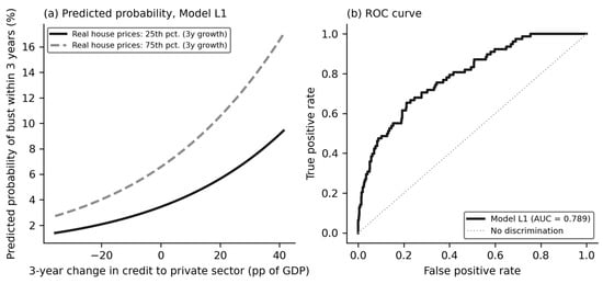
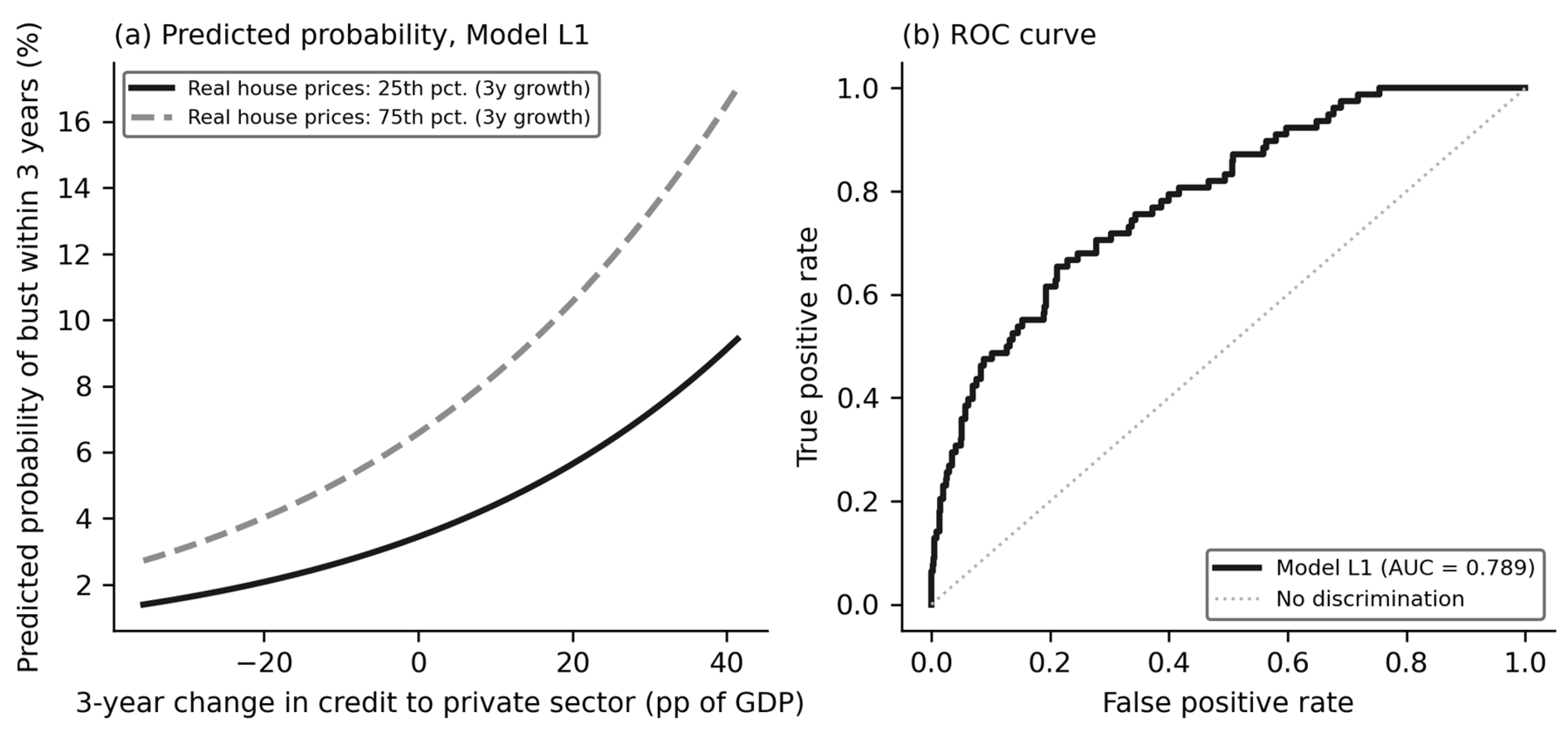
Figure 1 visualises these results. Figure 1a shows that the predicted probability of a bust rises from below 2 percent when the credit ratio has fallen by 35 points over three years to around 9 percent when it has risen by 40 points, holding real house price growth at its 25th percentile; along the 75th percentile of house price growth, the same range of credit expansion moves the probability from about 3 percent to 17 percent. The convexity of the curves and the widening gap between them illustrate the interaction between the two booms that Panel A of Table 3 captured in discrete form. Figure 1b plots the ROC curve of Model L1; the curve rises steeply at low false positive rates, which is the region that matters for policy, since a signal that captures half of the busts three years in advance at a false alarm rate of about 10 percent is operationally useful. Hypothesis H2 is therefore supported.

Figure 1. Predicted probability of a house price bust and discrimination of the baseline logistic model. Notes: Panel (a) plots the probability of a bust beginning within three years predicted by Model L1 as a function of the three-year change in the credit-to-GDP ratio, evaluated at the sample means of real GDP growth and the current account balance and at the 25th and 75th percentiles of three-year real house price growth. Panel (b) plots the receiver operating characteristic curve of Model L1. Source: authors’ calculations from BIS and World Bank data.

4.5. Busts and Bank Asset Quality

Table 6 turns to the consequences of busts-for-bank balance sheets. Model N1 regresses the annual change in the non-performing loan ratio on the in-bust indicator, real GDP growth, and unemployment with country fixed effects, on 780 observations from 55 economies. During a bust, the non-performing loan ratio increases by 1.4 percentage points per year more than in other periods after controlling for the cyclical position; the effect is significant at the 1 percent level with cluster-robust standard errors and even more precisely estimated with HC3 errors. A one-point lower real GDP growth raises the change in the ratio by 0.14 points and a one-point higher unemployment rate by 0.18 points, both significant. Model N2 adds the three-year change in the credit ratio lagged one year. The coefficient is 0.039 (p < 0.001): a credit expansion of 25 points of GDP over three years is followed by an additional increase of about one percentage point per year in the non-performing loan ratio, independently of whether a bust has started. The in-bust coefficient falls to 0.94 but remains significant at the 1 percent level, so that the effects of the bust and of the preceding credit expansion are cumulative. The R-squared rises from 0.24 to 0.32 when the credit variable is added.

Table 6. Fixed effects panel regressions for the annual change in the ratio of non-performing loans to gross loans (percentage points).

Regressor	Model N1	Model N2
House price bust in progress (dummy)	1.405 *** (0.509) [0.271]	0.937 *** (0.304) [0.228]
Change in credit/GDP, 3-year (t−1)	n/a	0.039 *** (0.008) [0.007]
Real GDP growth (%)	−0.137 *** (0.038) [0.033]	−0.126 *** (0.032) [0.031]
Unemployment rate (%)	0.179 ** (0.078) [0.054]	0.184 *** (0.070) [0.052]
Constant	−0.537 (0.358) [0.284]	−0.752 ** (0.342) [0.293]
Observations	780	780
Countries	55	55
R-squared	0.239	0.324
Country fixed effects	Yes	Yes

Notes: The dependent variable is the annual change in bank non-performing loans as a percentage of total gross loans. Entries are coefficients with standard errors clustered by country in parentheses and HC3 standard errors in square brackets; significance stars refer to the cluster-robust standard errors. *** p < 0.01, ** p < 0.05, n/a denotes that the variable is not included in the model. Source: authors’ calculations from World Bank World Development Indicators (IMF Financial Soundness Indicators) and BIS data.

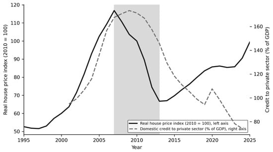
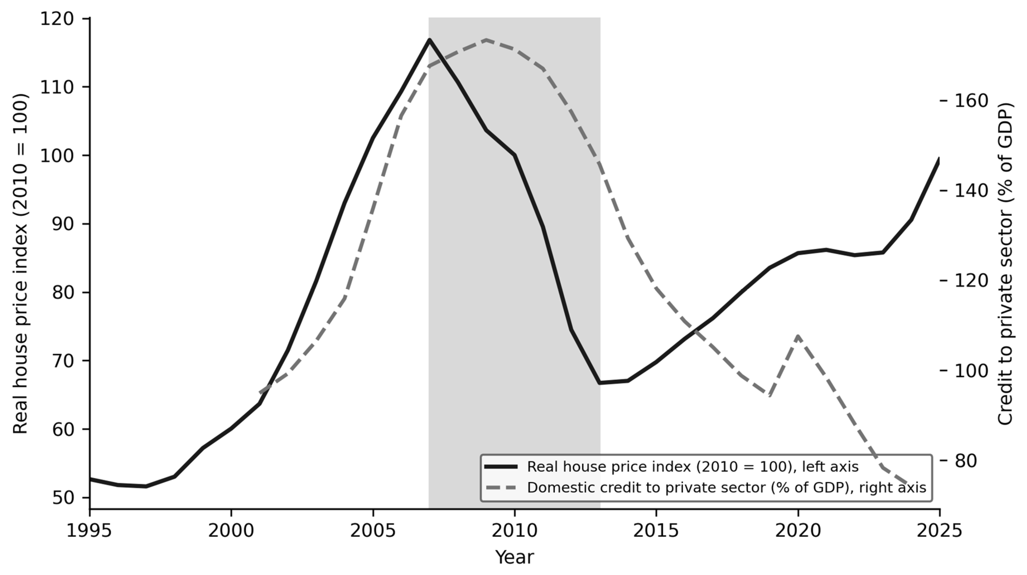
These results support Hypothesis H3 and close the circle of the argument. Credit expansion raises real house prices; the joint expansion of credit and prices raises the probability of a bust; and the bust, together with the preceding expansion, deteriorates the quality of bank assets. The Spanish experience shown in Figure 2 is the clearest illustration. Between 2001 and 2007, the ratio of credit to the private sector rose from 95 to 168 percent of GDP while the real house price index rose from 64 to 117; the peak of 2007 was followed by a six-year bust in which real prices fell by 43 percent, and the credit ratio, which continued to rise to 173 percent in 2009 as nominal GDP contracted, had fallen to 94 percent by 2019. The non-performing loan ratio, according to the WDI report for Spain from 2012, peaked at 7.1 percent in 2013 before declining steadily to below 3 percent. Since 2014, real house prices have recovered, but the credit ratio has continued to fall to 74 percent of GDP in 2024, so that the current expansion of Spanish house prices is, for the first time in decades, not being financed by an increase in leverage relative to income.

Figure 2. Real house prices and credit to the private sector in Spain, 1995 to 2025. Notes: The shaded area marks the bust episode identified by the algorithm of Section 3.2 (peak 2007, trough 2013, real decline of 42.9 percent). Sources: BIS-selected residential property price series (real index, 2010 = 100, annual averages of quarterly data); World Bank World Development Indicators, domestic credit to private sector (% of GDP), available from 2001.

4.6. Robustness: Country Groups and the Low Interest Rate Period

Because the sample of 57 economies is heterogeneous, we first re-estimate the baseline models separately for advanced economies (36), euro area members (20), advanced economies outside the euro area (16) and emerging economies (21), following the IMF World Economic Outlook classification. Table 7 shows that the lagged change in the credit-to-GDP ratio has a positive effect on real house price growth that is significant at the 1 percent level in every group, ranging from 0.14 in advanced economies outside the euro area to 0.18 in the euro area and 0.32 in emerging economies. The difference between emerging and advanced economies is not significant when tested in the pooled sample through an interaction term (p = 0.34). In the logistic models, both the three-year credit expansion and the three-year real house price growth raise the odds of a bust in all groups, and discrimination is highest in the euro area (AUC = 0.875) and in emerging economies (AUC = 0.852). The main results are therefore not driven by any particular group of countries.

Table 7. Robustness by country group.

Panel A. Fixed Effects Regressions For Real House Price Growth (Model M1)
Regressor	Full Sample	Advanced	Euro Area	Advanced, Non-Euro	Emerging
Change in credit/GDP (t−1)	0.174 *** (0.031) [0.031]	0.153 *** (0.031) [0.030]	0.182 *** (0.049) [0.059]	0.143 *** (0.041) [0.036]	0.317 *** (0.105) [0.101]
Real GDP growth (t−1)	0.481 *** (0.070) [0.068]	0.390 *** (0.080) [0.081]	0.504 *** (0.101) [0.115]	0.189 ** (0.085) [0.124]	0.697 *** (0.138) [0.123]
CPI inflation (t−1)	−0.173 (0.160) [0.176]	−0.592 *** (0.135) [0.118]	−0.487 *** (0.148) [0.151]	−0.791 *** (0.277) [0.182]	0.010 (0.141) [0.214]
Current account/GDP (t−1)	0.422 *** (0.089) [0.072]	0.393 *** (0.095) [0.072]	0.454 *** (0.173) [0.117]	0.328 *** (0.097) [0.092]	0.463 *** (0.156) [0.147]
Observations	1247	818	398	420	429
Countries	57	36	20	16	21
R-squared (within)	0.127	0.180	0.201	0.179	0.115
Country fixed effects	Yes	Yes	Yes	Yes	Yes
Panel B. Logistic Regressions for the Probability of a Bust Within Three Years (Model L1), Odds Ratios
Regressor	Full Sample	Advanced	Euro Area		Emerging
Change in credit/GDP, 3-year (pp)	1.026 *** [1.010, 1.043]	1.020 *** [1.005, 1.034]	1.079 *** [1.037, 1.123]		1.069 ** [1.002, 1.140]
Real house price growth, 3-year (%)	1.038 *** [1.019, 1.058]	1.055 *** [1.025, 1.085]	1.046 ** [1.005, 1.089]		1.031 *** [1.010, 1.052]
Current account (% GDP)	0.932 ** [0.872, 0.996]	0.952 [0.894, 1.014]	1.078 [0.954, 1.218]		0.877 [0.729, 1.055]
Observations/bust events	1021/78	664/50	311/29		357/28
Countries	57	36	20		21
AUC	0.791	0.783	0.875		0.852

Notes: Countries are classified following the IMF World Economic Outlook. Panel A: entries are coefficients with standard errors clustered by country in parentheses and HC3 standard errors in square brackets; significance stars refer to the cluster-robust standard errors. In the full sample with an interaction between the credit variable and an emerging economy dummy, the coefficient on credit is 0.165 (0.031) and the interaction is 0.092 (0.096), p = 0.34. Panel B: odds ratios with 95 percent confidence intervals based on standard errors clustered by country; real GDP growth and a constant are included but not shown. The full sample column re-estimates the baseline models with the BIS release of October 2026, and small differences from Table 4 and Table 5 reflect data revisions. *** p < 0.01, ** p < 0.05, Source: authors’ calculations from BIS and World Bank data.

Second, we examine whether the period of extremely low interest rates that followed the global financial crisis constitutes a distinct environment. We interact the credit variable with (i) a common indicator for the post-crisis low rate era, equal to one when the lagged regressors refer to 2009 to 2021; (ii) a country-specific indicator of the effective lower bound (ELB), equal to one when the annual average central bank policy rate is 0.5 percent or less (BIS dataset WS_CBPOL, using the ECB main refinancing rate for euro area members from the year of adoption of the euro); and (iii) the number of years at the effective lower bound during the previous three years, which allows for a delayed effect. Table 8 shows that the credit coefficient remains between 0.13 and 0.16 and is significant at the 1 percent level in all specifications, including one with year fixed effects. The low-rate environment raised real house price growth by about 2 percentage points per year, with a cumulative effect of about 0.5 points for each year spent at the lower bound, and in the 2009 to 2021 era the response of house prices to credit expansion was larger (0.26 against 0.14, an interaction which is significant at the 5 percent level); with the country-specific indicator, the interaction has the same sign but is not significant. In the logistic models, however, the low rate indicators and their interactions with credit are not significant (odds ratios of the interactions of 1.004 and 1.000) and leave the credit odds ratio unchanged (1.025 and 1.027). Low rates therefore amplified the transmission of credit to house prices without altering the link between credit and price booms and subsequent busts.

Table 8. Credit expansion and real house price growth in the low interest rate period.

Regressor	(1) Low-Rate Era, 2009 to 2021	(2) Country ELB (t−1)	(3) Years at ELB, t−3 to t−1	(4) Year Fixed Effects
Change in credit/GDP (t−1)	0.137 *** (0.035) [0.038]	0.152 *** (0.032) [0.035]	0.156 *** (0.032) [0.037]	0.130 *** (0.029) [0.026]
Low-rate indicator	0.347 (0.794) [0.567]	2.051 *** (0.597) [0.560]	0.467 ** (0.220) [0.179]	n/a
Credit x low-rate indicator	0.120 ** (0.059) [0.059]	0.085 (0.069) [0.071]	0.028 (0.029) [0.028]	n/a
Macroeconomic controls (t−1)	Yes	Yes	Yes	Yes
Country fixed effects	Yes	Yes	Yes	Yes
Year fixed effects	No	No	No	Yes
Observations	1247	1147	1083	1247
Countries	57	55	55	57

Notes: The dependent variable is annual real house price growth. Controls as in Model M1 (lagged real GDP growth, CPI inflation, and current account balance). ELB: effective lower bound, defined as an annual average central bank policy rate of 0.5 percent or less (BIS dataset WS_CBPOL; ECB main refinancing rate for euro area members). In column (3), the indicator counts the years at the ELB between t⁻³ and t⁻¹ (0 to 3). In the sample of columns (2) and (3), which excludes the two economies without policy rate data, the baseline credit coefficient without interactions is 0.161 (0.034). Entries are coefficients with standard errors clustered by country in parentheses and HC3 standard errors in square brackets. *** p < 0.01, ** p < 0.05, n/a denotes that the variable is not included in the model. Source: authors’ calculations from BIS and World Bank data.

4.7. Sensitivity to the Definition of Busts and to the Frequency of the Price Index

Table 9 re-estimates the baseline models under alternative definitions of a bust. Lowering the threshold to 10 percent raises the number of episodes from 37 to 52, and raising it to 20 percent reduces them to 26; shortening the horizon to four years or extending it to eight years yields 36 and 42 episodes. In all cases, the odds ratios of the three-year credit expansion (1.022 to 1.032) and of the three-year real house price growth (1.038 to 1.045) are very close to the baseline and significant at the 1 percent level, and the area under the ROC curve ranges from 0.77 to 0.85. A stricter threshold identifies fewer and deeper busts, which are easier to predict and more damaging for bank asset quality. Busts remain associated with a significant increase in the non-performing loan ratio in every case except with the four-year horizon, which truncates the longest and most costly episodes. Replacing the annual average of the price index with its fourth-quarter value, which dates turning points at the end of the year, leaves the results essentially unchanged; in this case, the coefficient of the lagged change in the credit ratio in Model M1 is 0.137 (0.028), significant at the 1 percent level.

Table 9. Sensitivity of the main results to the definition of busts and to the frequency of the price index.

Definition	Busts (Peak 1995 or Later)	Pre-Bust Years/Obs.	OR Credit, 3-Year	OR House Prices, 3-Year	AUC	NPL Change in Bust
Baseline: 15%, 6 years, annual average	37	78/1021	1.026 *** [1.010, 1.043]	1.038 *** [1.019, 1.058]	0.791	0.939 *** (0.301)
Threshold 10%	52	101/974	1.022 *** [1.008, 1.037]	1.041 *** [1.024, 1.059]	0.769	0.650 *** (0.234)
Threshold 20%	26	50/1064	1.028 *** [1.012, 1.045]	1.040 *** [1.021, 1.060]	0.842	1.115 *** (0.417)
Horizon 4 years	36	69/1071	1.032 *** [1.015, 1.050]	1.045 *** [1.024, 1.066]	0.846	0.486 (0.315)
Horizon 8 years	42	81/965	1.025 *** [1.009, 1.041]	1.040 *** [1.019, 1.062]	0.790	0.844 *** (0.267)
Fourth-quarter value instead of annual average	41	79/1018	1.027 *** [1.012, 1.043]	1.040 *** [1.020, 1.060]	0.789	0.706 ** (0.319)

Notes: ORs are odds ratios from the baseline logistic Model L1 with 95 percent confidence intervals based on standard errors clustered by country. NPL change in bust is the coefficient on the bust-in-progress indicator in Model N2 (annual change in the non-performing loan ratio), with standard errors clustered by country in parentheses. The baseline uses the catalogue of Table 1; the alternative definitions apply the algorithm of Section 3.2 with the parameters indicated to the BIS release of October 2026. *** p < 0.01, ** p < 0.05, Source: authors’ calculations from BIS and World Bank data.

5. Discussion

5.1. Interpretation of the Main Findings

The evidence assembled in this paper points consistently in the same direction. Credit expansion is the variable that most robustly predicts real house price growth, the probability of a bust, and the subsequent deterioration of bank balance sheets. The magnitude of the effects is economically meaningful. A country that increases its credit-to-GDP ratio by 25 points over three years while its real house prices rise by 25 percent—which is roughly what Spain, Ireland and the Baltic states experienced before 2007 and what several advanced economies experienced in more mildly between 2019 and 2022—faces a probability of a bust within three years that our baseline model places at around 15 percent, roughly twice the unconditional rate of 7.7 percent; if the bust materialises, the non-performing loan ratio can be expected to rise by roughly two percentage points per year over its normal path for the duration of the correction. Section 4.6 shows that these regularities are not specific to any group of countries: they hold in advanced economies, in the euro area and in emerging economies, and the credit effect remains when the post-crisis period of very low interest rates is taken into account.

These regularities are what the Austrian theory of the credit cycle predicts. The temporal ordering in Table 4, in which lagged credit growth explains current real house price growth, is consistent with the causal direction from credit expansion to relative price distortion that von Mises (1912/1953) and Hayek (1931) described, and with the specific role of long-lived assets emphasised by Huerta de Soto (2006) and Garrison (2001). The finding that the credit effect survives the inclusion of broad money growth is particularly relevant because it separates the credit channel, which operates through the lending decisions of banks and the resulting distortion of the interest rate, from the aggregate quantity of money; the Austrian account is a theory of credit expansion, not of inflation in general. The interaction between credit booms and price booms documented in Table 3 and Table 5 corresponds to the phase of the cycle in which the rise in collateral values validates further lending, the process that Minsky (1986) described as the migration towards speculative finance and that Kiyotaki and Moore (1997) and Bernanke et al. (1999) formalised as the financial accelerator. The lagged deterioration of bank asset quality in Table 6 is the liquidation phase in which malinvestment is recognised, and the additional effect of the preceding credit expansion on non-performing loans, over and above the effect of the bust itself, indicates that the losses are proportional to the excess that was accumulated, which is the central prediction of the theory.

Our results are also consistent with the empirical financial cycle literature. The predictive power of three-year credit growth for busts mirrors the findings of Schularick and Taylor (2012), Jordà et al. (2015) and Dell’Ariccia et al. (2016) for financial crises, and the improvement in discrimination obtained by combining credit and house price indicators reproduces the result of Anundsen et al. (2016) and of Borio and Lowe (2002). The area under the ROC curve of 0.79 for the baseline model is in the range reported by Drehmann and Juselius (2014) for the credit-to-GDP gap as a predictor of banking crises, although our outcome variable is a house price bust rather than a systemic banking crisis, which is a more frequent and less extreme event. The role of the current account deficit as an additional risk factor confirms the twin crises mechanism of Kaminsky and Reinhart (1999) and the results of Gourinchas and Obstfeld (2012): booms financed by foreign saving are more fragile because the reversal of capital flows can force an abrupt tightening of credit conditions that domestic banks cannot offset.

5.2. Unexpected Findings

Three results deserve comment because they were not fully anticipated. The first is the weak performance of the real interest rate. The Austrian theory attributes the boom to an interest rate below its natural level, and the financial cycle literature generally finds that low real rates precede booms. In our data, the real interest rate has the expected negative sign both in the house price growth regression and in the bust logit, but the coefficients are imprecisely estimated, and the sample is reduced by more than half. Two explanations are plausible. First, the WDI real interest rate is derived from the average lending rate deflated by the GDP deflator and is not reported for most euro area members after 1999, precisely the economies where the divergence between a common nominal policy rate and heterogeneous national inflation produced the largest real rate dispersion (Jiménez et al., 2014). Second, and more fundamentally, the relevant magnitude in the theory is not the level of the real rate, but its deviation from the unobservable natural rate, which the level of the rate captures only imperfectly; the quantity of credit created is a better observable proxy for that deviation, which is precisely why the credit variables perform so well. The result therefore does not contradict the theory but rather illustrates the measurement difficulty that has accompanied it since Wicksell.

The second unexpected finding is that real GDP growth is not significantly associated with the probability of a bust, and that pre-bust years display, if anything, higher growth than other years. This reinforces the point that busts are not the consequence of a deterioration of fundamentals but of an excess built during the boom: the economy grows fast precisely because credit is expanding, and the growth conceals the vulnerability. Policymakers who calibrate risk on the basis of current output growth will systematically underestimate it. The third finding is the composition of the third wave of busts. Whereas the 2007 wave was concentrated in economies with large current account deficits and rapid credit growth, the 2022 wave affected economies with current account surpluses and moderate credit growth, such as Germany, Sweden, Finland and Luxembourg, in which the boom had been driven mainly by an exceptionally long period of negative real rates rather than by an acceleration of leverage. These episodes are shallower and, so far, have not been accompanied by a comparable deterioration of bank asset quality, which suggests that the depth of a bust depends on the leverage accumulated during the boom rather than on the price rise alone, in line with Jordà et al. (2015). The robustness exercises of Section 4.6 support this interpretation: being at the effective lower bound raised real house price growth independently of credit, and the effect accumulated with the time spent at the bound.

5.3. Policy Implications

The findings have direct implications for the design of countercyclical macroprudential policy. The credit-to-GDP gap is already the reference indicator for the countercyclical capital buffer under Basel III, and our results confirm that the three-year change in the credit ratio is a powerful predictor of housing busts. However, the substantial improvement in discrimination obtained by adding real house price growth, and the disproportionate bust rate when both indicators signal a boom, argue for a dual indicator approach in which the buffer, loan-to-value limits, and debt service-to-income limits are activated when credit and house prices boom together. Cerutti et al. (2017a) and Akinci and Olmstead-Rumsey (2018) show that such instruments are effective in dampening credit and house price growth, especially in advanced economies. The results on non-performing loans also imply that provisioning and capital requirements should be forward-looking and calibrated to the credit expansion of the preceding years, since the eventual losses are proportional to that expansion. From the perspective of the Austrian theory, these instruments treat the symptoms of a process whose origin lies in the capacity of the banking system to expand credit beyond saving; the most reliable remedy is a monetary framework that does not systematically hold the market rate below the natural rate for extended periods, but in the absence of such a framework the countercyclical tools examined here are the second best.

5.4. Limitations

Several limitations should be borne in mind, in addition to the measurement issues discussed in Section 3.5. First, the analysis uses aggregate data, which cannot capture the heterogeneity of borrowers that Mian and Sufi (2009) exploit with microdata. Second, although Section 4.7 shows that the results are robust to alternative thresholds and horizons, the identification of busts rests on a convention, and alternative choices shift some marginal episodes. Third, the panel regressions establish predictive, not causal, relations; the use of lagged regressors and country fixed effects mitigates but does not eliminate the possibility of reverse causation through expectations of future price growth that induce both borrowing and lending. Finally, write-offs and asset transfers, such as the transfer of Spanish real estate assets to the asset management company in 2012, can reduce the measured non-performing loan ratio without any improvement in underlying quality.

6. Conclusions

This paper has used official data from the Bank for International Settlements and the World Bank for 57 economies between 1995 and 2025 to test three hypotheses on the relation between credit expansion, house price cycles and financial stability. The answer to each of them is as follows.

H1 is supported. Credit expansion raises subsequent real house price growth: each percentage point of GDP added to private credit raises real house price growth in the following year by 0.17 to 0.21 points, and the effect remains significant when broad money growth, the real interest rate, or year fixed effects are included in advanced, euro area, and emerging economies and during the post-crisis low interest rate period, when it was larger.

H2 is supported. The probability that a bust begins within three years increases with the preceding three-year expansion of credit (odds ratio 1.026 per percentage point of GDP) and of real house prices (1.038 per percent), and a model with these variables discriminates between pre-bust and other years with an area under the ROC curve of about 0.8. The odds of a bust are 3.8 times higher after a credit boom and 2.4 times higher after a house price boom, and when both booms coincide, the bust rate within three years is 30 percent, compared to 5 percent otherwise. These results hold for alternative definitions of a bust.

H3 is supported. During busts, the non-performing loan ratio rises by about one percentage point per year more than in other periods, and a credit expansion of 25 points of GDP over three years adds about one further point per year, so that the losses are larger the greater the preceding expansion. The result holds for all bust definitions except the shortest four-year horizon, which truncates the longest episodes.

These regularities are those predicted by the Austrian theory of the credit cycle and are consistent with the modern financial cycle literature. The sequence of credit expansion, relative price distortion in the most interest-sensitive asset, boom, bust, and liquidation is visible in the aggregate data of a large and heterogeneous set of economies over three decades and three waves of busts. The policy implication is that financial stability cannot be assessed from current output growth or from the level of interest rates alone; it requires the monitoring of the joint dynamics of credit and property prices and the willingness to act countercyclically when both signal a boom, through capital buffers, borrower-based measures, and forward-looking provisioning calibrated to the accumulated expansion.

Future research could extend the analysis in four directions. The use of the BIS total credit statistics would allow the separation of household and corporate credit and the identification of the mortgage component, at the cost of a smaller sample. Quarterly data and duration models could refine the timing of turning points and estimate the expected time to a bust rather than its probability within a fixed window. The comparison between the 2007 and the 2022 waves, in which the role of leverage and the length of the low-rate period differed markedly, offers a natural setting in which to test whether the depth of a correction is determined by the credit expansion or by the interest rate distortion that preceded it, a question on which the Austrian theory and the leverage cycle literature make partly different predictions. Finally, the post-crisis period of interest rates at the effective lower bound, whose effects on house prices we document in Section 4.6, deserves a dedicated study in which the shadow rate or the deviation of the policy rate from estimates of the natural rate is used to measure the stance of monetary policy more precisely.

References

- Adrian, T., & Shin, H. S. (2010). Liquidity and leverage. Journal of Financial Intermediation, 19(3), 418–437. [Google Scholar] [CrossRef] [Scilit]
- Agnello, L., & Schuknecht, L. (2011). Booms and busts in housing markets: Determinants and implications. Journal of Housing Economics, 20(3), 171–190. [Google Scholar] [CrossRef] [Scilit]
- Aikman, D., Haldane, A. G., & Nelson, B. D. (2015). Curbing the credit cycle. The Economic Journal, 125(585), 1072–1109. [Google Scholar] [CrossRef] [Scilit]
- Akin, O., Montalvo, J. G., García Villar, J., Peydró, J. L., & Raya, J. M. (2014). The real estate and credit bubble: Evidence from Spain. SERIEs, 5(2), 223–243. [Google Scholar] [CrossRef] [Scilit]
- Akinci, O., & Olmstead-Rumsey, J. (2018). How effective are macroprudential policies? An empirical investigation. Journal of Financial Intermediation, 33, 33–57. [Google Scholar] [CrossRef] [Scilit]
- Alonso Neira, M. A., Bagus, P., & Rallo Julián, J. R. (2011). Teorías del ciclo económico: Principales contribuciones y análisis a la luz de las aportaciones de la escuela austriaca de economía. Información Comercial Española, ICE: Revista de Economía, 858, 71–87. [Google Scholar]
- Anundsen, A. K., Gerdrup, K., Hansen, F., & Kragh-Sørensen, K. (2016). Bubbles and crises: The role of house prices and credit. Journal of Applied Econometrics, 31(7), 1291–1311. [Google Scholar] [CrossRef] [Scilit]
- Bagus, P., & Howden, D. (2010). The term structure of savings, the yield curve, and maturity mismatching. Quarterly Journal of Austrian Economics, 13(3), 64–85. [Google Scholar]
- Banco de España. (2017). Report on the financial and banking crisis in Spain, 2008–2014. Banco de España. [Google Scholar]
- Bank for International Settlements. (2026). Central bank policy rates (dataset WS_CBPOL). BIS Data Portal. Available online: https://data.bis.org (accessed on 2 September 2026).
- Bernanke, B. S., Gertler, M., & Gilchrist, S. (1999). The financial accelerator in a quantitative business cycle framework. In J. B. Taylor, & M. Woodford (Eds.), Handbook of macroeconomics (Vol. 1, pp. 1341–1393). Elsevier. [Google Scholar] [CrossRef] [Scilit]
- Bordo, M. D., & Jeanne, O. (2002). Monetary policy and asset prices: Does ‘benign neglect’ make sense? International Finance, 5(2), 139–164. [Google Scholar] [CrossRef] [Scilit]
- Borio, C. (2014). The financial cycle and macroeconomics: What have we learnt? Journal of Banking & Finance, 45, 182–198. [Google Scholar] [CrossRef] [Scilit]
- Borio, C., & Lowe, P. (2002). Asset prices, financial and monetary stability: Exploring the nexus (BIS Working Papers No. 114). Bank for International Settlements. [Google Scholar]
- Bracke, P. (2013). How long do housing cycles last? A duration analysis for 19 OECD countries. Journal of Housing Economics, 22(3), 213–230. [Google Scholar] [CrossRef] [Scilit]
- Brunnermeier, M. K., & Oehmke, M. (2013). Bubbles, financial crises, and systemic risk. In G. M. Constantinides, M. Harris, & R. M. Stulz (Eds.), Handbook of the Economics of Finance (Vol. 2, pp. 1221–1288). Elsevier. [Google Scholar] [CrossRef] [Scilit]
- Cameron, A. C., & Miller, D. L. (2015). A practitioner’s guide to cluster-robust inference. Journal of Human Resources, 50(2), 317–372. [Google Scholar] [CrossRef] [Scilit]
- Case, K. E., & Shiller, R. J. (2003). Is there a bubble in the housing market? Brookings Papers on Economic Activity, 2003(2), 299–362. [Google Scholar] [CrossRef] [Scilit]
- Cerutti, E., Claessens, S., & Laeven, L. (2017a). The use and effectiveness of macroprudential policies: New evidence. Journal of Financial Stability, 28, 203–224. [Google Scholar] [CrossRef] [Scilit]
- Cerutti, E., Dagher, J., & Dell’Ariccia, G. (2017b). Housing finance and real-estate booms: A cross-country perspective. Journal of Housing Economics, 38, 1–13. [Google Scholar] [CrossRef] [Scilit]
- Claessens, S., Kose, M. A., & Terrones, M. E. (2012). How do business and financial cycles interact? Journal of International Economics, 87(1), 178–190. [Google Scholar] [CrossRef] [Scilit]
- Dell’Ariccia, G., Igan, D., Laeven, L., & Tong, H. (2016). Credit booms and macrofinancial stability. Economic Policy, 31(86), 299–355. [Google Scholar] [CrossRef] [Scilit]
- Dembiermont, C., Drehmann, M., & Muksakunratana, S. (2013). How much does the private sector really borrow? A new database for total credit to the private non-financial sector. BIS Quarterly Review, 65–81. [Google Scholar]
- Drehmann, M., Borio, C., & Tsatsaronis, K. (2012). Characterising the financial cycle: Don’t lose sight of the medium term! (BIS Working Papers No. 380). Bank for International Settlements. [Google Scholar]
- Drehmann, M., & Juselius, M. (2014). Evaluating early warning indicators of banking crises: Satisfying policy requirements. International Journal of Forecasting, 30(3), 759–780. [Google Scholar] [CrossRef] [Scilit]
- Favara, G., & Imbs, J. (2015). Credit supply and the price of housing. American Economic Review, 105(3), 958–992. [Google Scholar] [CrossRef] [Scilit]
- Garrison, R. W. (2001). Time and money: The macroeconomics of capital structure. Routledge. [Google Scholar]
- Glaeser, E. L., Gyourko, J., & Saiz, A. (2008). Housing supply and housing bubbles. Journal of Urban Economics, 64(2), 198–217. [Google Scholar] [CrossRef] [Scilit]
- Glaeser, E. L., & Nathanson, C. G. (2017). An extrapolative model of house price dynamics. Journal of Financial Economics, 126(1), 147–170. [Google Scholar] [CrossRef] [Scilit]
- Gourinchas, P. O., & Obstfeld, M. (2012). Stories of the twentieth century for the twenty-first. American Economic Journal: Macroeconomics, 4(1), 226–265. [Google Scholar] [CrossRef] [Scilit]
- Hanley, J. A., & McNeil, B. J. (1982). The meaning and use of the area under a receiver operating characteristic (ROC) curve. Radiology, 143(1), 29–36. [Google Scholar] [CrossRef] [Scilit] [PubMed]
- Harding, D., & Pagan, A. (2002). Dissecting the cycle: A methodological investigation. Journal of Monetary Economics, 49(2), 365–381. [Google Scholar] [CrossRef] [Scilit]
- Hayek, F. A. (1931). Prices and production. Routledge. [Google Scholar]
- Hayek, F. A. (1933). Monetary theory and the trade cycle. Jonathan Cape. [Google Scholar]
- Himmelberg, C., Mayer, C., & Sinai, T. (2005). Assessing high house prices: Bubbles, fundamentals and misperceptions. Journal of Economic Perspectives, 19(4), 67–92. [Google Scholar] [CrossRef] [Scilit]
- Hott, C. (2011). Lending behavior and real estate prices. Journal of Banking & Finance, 35(9), 2429–2442. [Google Scholar] [CrossRef] [Scilit]
- Huerta de Soto, J. (2006). Money, bank credit, and economic cycles. Ludwig von Mises Institute. [Google Scholar]
- International Organization for Standardization. (2020). Codes for the representation of names of countries and their subdivisions—Part 1: Country code (ISO Standard No. 3166-1:2020). International Organization for Standardization.
- Jiménez, G., Ongena, S., Peydró, J. L., & Saurina, J. (2014). Hazardous times for monetary policy: What do twenty-three million bank loans say about the effects of monetary policy on credit risk-taking? Econometrica, 82(2), 463–505. [Google Scholar] [CrossRef] [Scilit]
- Jordà, Ò., Schularick, M., & Taylor, A. M. (2015). Leveraged bubbles. Journal of Monetary Economics, 76, S1–S20. [Google Scholar] [CrossRef] [Scilit]
- Jordà, Ò., Schularick, M., & Taylor, A. M. (2016). The great mortgaging: Housing finance, crises and business cycles. Economic Policy, 31(85), 107–152. [Google Scholar] [CrossRef] [Scilit]
- Justiniano, A., Primiceri, G. E., & Tambalotti, A. (2019). Credit supply and the housing boom. Journal of Political Economy, 127(3), 1317–1350. [Google Scholar] [CrossRef] [Scilit] [PubMed]
- Kaminsky, G. L., & Reinhart, C. M. (1999). The twin crises: The causes of banking and balance-of-payments problems. American Economic Review, 89(3), 473–500. [Google Scholar] [CrossRef] [Scilit]
- Kindleberger, C. P., & Aliber, R. Z. (2005). Manias, panics and crashes: A history of financial crises (5th ed.). Palgrave Macmillan. [Google Scholar]
- Kiyotaki, N., & Moore, J. (1997). Credit cycles. Journal of Political Economy, 105(2), 211–248. [Google Scholar] [CrossRef] [Scilit]
- Laeven, L., & Valencia, F. (2020). Systemic banking crises database II. IMF Economic Review, 68(2), 307–361. [Google Scholar] [CrossRef] [Scilit]
- Mian, A., & Sufi, A. (2009). The consequences of mortgage credit expansion: Evidence from the U.S. mortgage default crisis. The Quarterly Journal of Economics, 124(4), 1449–1496. [Google Scholar] [CrossRef] [Scilit]
- Mian, A., Sufi, A., & Verner, E. (2017). Household debt and business cycles worldwide. The Quarterly Journal of Economics, 132(4), 1755–1817. [Google Scholar] [CrossRef] [Scilit]
- Minsky, H. P. (1986). Stabilizing an unstable economy. Yale University Press. [Google Scholar]
- Nagelkerke, N. J. D. (1991). A note on a general definition of the coefficient of determination. Biometrika, 78(3), 691–692. [Google Scholar] [CrossRef]
- Phillips, P. C. B., Shi, S., & Yu, J. (2015). Testing for multiple bubbles: Historical episodes of exuberance and collapse in the S&P 500. International Economic Review, 56(4), 1043–1078. [Google Scholar] [CrossRef] [Scilit]
- Ravier, A. O., & Lewin, P. (2012). The subprime crisis. Quarterly Journal of Austrian Economics, 15(1), 45–74. [Google Scholar]
- Reinhart, C. M., & Rogoff, K. S. (2009). This time is different: Eight centuries of financial folly. Princeton University Press. [Google Scholar]
- Scatigna, M., Szemere, R., & Tsatsaronis, K. (2014). Residential property price statistics across the globe. BIS Quarterly Review, 61–76. [Google Scholar]
- Schularick, M., & Taylor, A. M. (2012). Credit booms gone bust: Monetary policy, leverage cycles, and financial crises, 1870–2008. American Economic Review, 102(2), 1029–1061. [Google Scholar] [CrossRef] [Scilit]
- Shiller, R. J. (2015). Irrational exuberance (3rd ed.). Princeton University Press. [Google Scholar]
- Stiglitz, J. E. (1990). Symposium on bubbles. Journal of Economic Perspectives, 4(2), 13–18. [Google Scholar] [CrossRef] [Scilit]
- von Mises, L. (1953). The theory of money and credit (H. E. Batson, Trans.). Yale University Press. (Original work published 1912). [Google Scholar]
- Wooldridge, J. M. (2010). Econometric analysis of cross section and panel data (2nd ed.). MIT Press. [Google Scholar]
Disclaimer/Publisher’s Note: The statements, opinions and data contained in all publications are solely those of the individual author(s) and contributor(s) and not of MDPI and/or the editor(s). MDPI and/or the editor(s) disclaim responsibility for any injury to people or property resulting from any ideas, methods, instructions or products referred to in the content. |
© 2026 by the authors. Licensee MDPI, Basel, Switzerland. This article is an open access article distributed under the terms and conditions of the Creative Commons Attribution (CC BY) license.