


Abstract
This study examines whether corporate information supplements management dividend forecasts in predicting dividend increases and whether the predictions improve stock selection in Japan. Using financial and market indicators, management forecasts, and dividend histories available at each prediction date, we develop machine learning models for Tokyo Stock Exchange firms with March fiscal year-ends, excluding banks. A rolling training, validation, and retraining procedure produces out-of-sample predictions for 2013–2023, with portfolio evaluation from June 2013 to May 2024. We compare forecast-based benchmarks and multivariate models. Then, we combine predicted probabilities with forecast dividend yields. Multivariate eXtreme Gradient Boosting (XGBoost) achieves a mean annual area under the receiver operating characteristic curve of 0.86, compared with 0.77 for XGBoost using only the forecast dividend yield change. The combined long–short strategy achieves an annualized Sharpe ratio of 1.26 and a positive alpha under the Fama–French three-factor model (t = 4.12, p < 0.001). Its arithmetic cumulative spread return remains positive under the examined transaction cost scenarios. These findings suggest that dividend increase predictions can complement forecast dividend yields in stock selection, whereas practical implementation requires consideration of borrowing costs and other trading constraints not separately assessed here.
1. Introduction
In recent years, listed firms have been increasingly called upon to improve their capital efficiency. Figure A1 in Appendix A separately shows the percentages of firms with a return on equity (ROE) below 8% and with a price-to-book ratio (PBR) below 1, highlighting challenges in enhancing firm value and returning capital to shareholders. Against this background, in March 2023, the Tokyo Stock Exchange (TSE) called on all companies listed on the Prime and Standard Markets to implement management practices conscious of the cost of capital and stock prices.
Dividend increases and share repurchases have attracted attention as measures for improving capital efficiency. Dividend increases, in particular, are shareholder payout measures that firms are more likely to choose when they are confident in stable future earnings and cash flows; they are therefore regarded as important decisions reflecting a firm’s stance and outlook. In recent years, moves to strengthen shareholder payouts through dividend increases have accelerated amid public concern about the accumulation of retained earnings and market calls for improved capital efficiency.
Dividend increases also serve multiple functions beyond returning funds to shareholders, including the appropriate use of surplus funds, adjustment of capital structure, and signaling a firm’s future outlook to the market. From a theoretical perspective, Jensen (1986) noted that excessive free cash flow within a firm may lead managers to undertake inefficient reinvestments, thereby eroding shareholder value. Returning funds to shareholders through dividend increases is an effective way to mitigate such agency problems. In addition, the asymmetric-information models of Bhattacharya (1979) and Miller and Rock (1985) show that dividend policy functions as a signaling mechanism that indirectly conveys information held within the firm to the market.
Dividend increases have also attracted attention because of their effects on stock prices. Julio and Ikenberry (2004) show that the market responds favorably to resumed or increased dividends. In Japan, Uchiyama and Takahashi (2015) document pronounced positive stock-price reactions to dividend-increase announcements.
These reactions suggest that dividend increases function as a clear positive signal in the Japanese market, where firms tend to manage dividend policy with a long-term emphasis on stability.
In contrast, share repurchases are a major shareholder payout measure but have a decision-making structure different from that of dividend increases. In particular, although dividend increases involve rigidity in that “a dividend level, once raised, cannot easily be lowered,” share repurchases tend to be implemented flexibly in response to business cycles and stock-price levels (Jagannathan et al., 2000). Consequently, dividend increases reflect long-term judgments about firms’ permanent earning capacity, whereas share repurchases are often based on short-term factors, such as stock-price undervaluation or temporary surplus funds. Another distinctive feature of dividend increases is that firms disclose forecast dividends in advance. Forecast dividends provide important information to investors, but managers tend to set them conservatively, and actual dividends frequently exceed forecast amounts. Therefore, forecast dividends alone may not fully explain the occurrence of dividend increases.
Mochizuki et al. (2026) show that share repurchase behavior can be predicted using firm-level financial, market, governance, and historical repurchase information and that the resulting predicted probabilities can be applied to stock selection. They provide a framework in which a shareholder payout decision is first predicted and the prediction is then evaluated as a stock selection signal. However, in the case of dividend increases, two unresolved issues remain. First, firms disclose forecast dividends before the realized dividend is known; therefore, investors already observe a management-based signal of future dividend decisions. Consequently, it is unclear whether firm-level information provides additional predictive information beyond management dividend forecasts. Second, forecast dividend yield is already a conventional stock selection measure based on expected dividend income. Even if future dividend increases can be predicted, it remains unclear whether the predicted probability provides information that complements this existing measure. These two unresolved issues motivate the following two research questions of this study.
First, to what extent can machine learning models combining financial and market indicators with historical dividend information improve the prediction of future dividend increases relative to approaches based on management dividend forecasts? Second, can combining predicted dividend increase probabilities with forecast dividend yields improve portfolio performance relative to strategies using either measure alone?
To address the first research question, we augment the financial, market, and governance indicators used in the share repurchase prediction framework with dividend-specific information, including historical dividend changes, positive and negative dividend surprises, and historical dividend yields. We compare the resulting multivariate models with management-forecast-based benchmarks and use feature importance and SHapley Additive exPlanations (SHAP) values to examine the information contributing to the predictions. To address the second research question, we combine predicted dividend increase probabilities with forecast dividend yields and compare the resulting strategy with strategies using either measure alone. Thus, this study extends the prior prediction framework by examining the incremental predictive information specific to dividend increases and its potential value in dividend-yield-based stock selection. The analysis concerns predictive associations and does not identify causal effects underlying dividend increase decisions.
2. Literature Review
Building on prior research on the determinants of dividend-increase behavior and its effects on stock prices, this study seeks to predict dividend-increase behavior using machine learning and applies the resulting predictions to equity portfolio management. This section reviews the relevant literature in four categories: theoretical foundations common to dividends and share repurchases, distinctive characteristics of and research on share repurchases, distinctive characteristics of and research on dividend increases, and related research using machine learning.
2.1. Common Theoretical Foundations of Dividends and Share Repurchases
Dividends and share repurchases are shareholder payout measures that share two principal theoretical foundations: agency theory and signaling theory. First, Jensen’s (1986) free cash flow hypothesis plays a central role in agency theory. This hypothesis argues that when excessive funds accumulate within a firm, managers may direct them toward inefficient investment or organizational expansion, potentially impairing shareholder value. Therefore, dividends and share repurchases are mechanisms for distributing surplus funds outside the firm and reducing agency costs. Recent evidence is consistent with this agency-based interpretation. Kim et al. (2024) find that dividend payments reduce managerial bad news hoarding and overinvestment, providing empirical evidence that dividend payouts can constrain managerial behavior associated with agency problems.
Second, according to Bhattacharya (1979) and Miller and Rock (1985), signaling theory emphasizes that dividends and share repurchases can convey a firm’s private information about future earning capacity. Strengthening shareholder payouts can therefore communicate managerial confidence and earnings outlooks to investors. Chang et al. (2024) examine how management forecasting ability affects the information conveyed by dividends. They find that the positive association between dividend increases and subsequent earnings improvements among Japanese firms is stronger when managers have greater earnings forecasting ability. This finding indicates that the information about future earnings contained in dividend changes depends on management forecasting ability.
Moreover, these theoretical arguments have empirical support. Grullon et al. (2002) and Uchiyama and Takahashi (2015) report positive abnormal returns following dividend increase announcements. Ikenberry et al. (1995) report medium- to long-term excess returns following share repurchase announcements. Furthermore, recent studies provide evidence that both forms of shareholder payout are associated with positive stock market reactions. Michałowski (2025) reports a statistically significant positive abnormal return of 1.39% for dividend increases on the Warsaw Stock Exchange. Similarly, Anolick et al. (2021) report positive cumulative abnormal returns for a large sample of open market share repurchases across nine European countries. Despite these commonalities, dividends and share repurchases differ substantially in their decision-making structures and implementation timing. The next subsection summarizes the characteristics specific to share repurchases and clarifies how they differ from dividend policy.
2.2. Distinctive Characteristics of Share Repurchases and Related Research
Like dividends, share repurchases are shareholder payout measures, but their decision-making processes have distinctive characteristics. Jagannathan et al. (2000) point out that share repurchases can be adjusted flexibly in response to business cycles and stock-price levels, whereas dividends exhibit rigidity because firms are expected to maintain a dividend level once it has been increased. Share repurchases therefore tend to be used for more flexible purposes, such as responding to temporary cash surpluses or correcting perceived stock-price undervaluation. Arena and Julio (2023) provide evidence of this flexibility: firms facing greater litigation risk reduce dividends and shift payout toward share repurchases, whereas cash-constrained firms reduce repurchases when settlement costs are realized.
Empirical studies have confirmed that share repurchases are sensitive to external conditions and market valuations. Vermaelen (1981) shows that share repurchases function as a signal of firm undervaluation and reports that repurchase activity increases when firms perceive their shares to be undervalued. Focusing on changes in ownership structure, Kitamura and Kojima (2019) show that, for regional banks, the probability of a share repurchase rises as foreign institutional ownership increases. This finding provides an example of shareholder monitoring pressure and governance demands influencing managerial behavior and supports the view that share repurchases are affected not only by market valuation but also by ownership structure. More recently, Bourveau et al. (2023) show that institutional-investor behavior can also affect repurchase decisions through market valuation: selling by short-term-oriented mutual funds can create undervaluation, to which portfolio firms respond by increasing share repurchases.
Mochizuki et al. (2026) use machine-learning models to predict share-repurchase behavior among Japanese firms and calculate feature importance to analyze factors underlying the decision-making process. According to the feature importance results, “share repurchase yield (past year)” is the most important variable, followed by variables capturing prior share-repurchase activity. These results suggest strong persistence in share-repurchase behavior. “Foreign ownership ratio,” “market capitalization,” “equity ratio,” and “PBR” also show non-negligible importance, indicating that external-investor pressure, market valuation, and financial soundness are relevant to the decision. Furthermore, they apply the predicted share repurchase probabilities directly to stock selection by constructing portfolios ranked by the model outputs. This provides a prediction-to-portfolio framework that this study extends using the predicted probability as an additional screening dimension (rather than as the sole stock selection signal) within a strategy based on forecast dividend yield.
Together, the prior literature suggests that share-repurchase decisions are often based on short-term factors that depend on the external environment. By contrast, dividend increases appear to reflect more long-term, structural judgments; the next subsection summarizes their distinctive characteristics.
2.3. Distinctive Characteristics of Dividend Increases and Related Research
Although dividend increases and share repurchases are both shareholder payout measures, their decision-making structures differ fundamentally. First, dividend policy exhibits strong rigidity because firms are expected to maintain a dividend level once it has been increased. Lintner (1956) shows that firms tend to base dividend-increase decisions on permanent earning capacity rather than temporary profits, indicating that such decisions are made cautiously and from a long-term perspective. Lin and Yu (2025) examine managerial characteristics associated with downward dividend stickiness. They find that overconfident CEOs increase dividends more when earnings rise but reduce them less when earnings fall, linking asymmetric dividend adjustments to managerial overconfidence. Drawing on life-cycle theory, DeAngelo et al. (2006) report that mature firms tend to favor dividend increases as retained earnings accumulate and growth opportunities decline. Additionally, Akindayomi and Amin (2022) provide recent evidence that firms’ longer-term strategic characteristics are related to dividend increase decisions. They find that innovation-oriented firms are less likely to increase dividends than cost-efficiency-oriented firms, with the difference being more pronounced among growth firms. Taken together, these studies suggest that dividend increases are associated with persistent earnings capacity, managerial characteristics, corporate life cycle conditions, and longer-term strategic orientation, consistent with the view that dividend increase decisions are relatively rigid and structural compared with more flexible payout measures such as share repurchases.
Second, a notable feature of dividend increases in the Japanese market is the existence of forecast dividends. Forecast dividends are the dividend amounts that a firm’s management expects to pay, based on its assessment of the firm’s condition and prospects. However, managers tend to set forecast dividends conservatively in light of future uncertainty, and actual dividends commonly exceed forecast amounts when financial results are finalized. It therefore remains unclear to what extent forecast dividends reflect managers’ private information, and forecast values alone have limited ability to explain the occurrence of dividend increases. Understanding dividend-increase decisions thus requires consideration of diverse factors not fully captured by forecast dividends, including complex relationships among financial indicators, corporate governance structures, and firms’ stages of growth. However, much of the existing literature focuses on stock-price reactions following dividend-increase announcements or descriptions of firm characteristics, leaving scope to examine whether firm-level information provides incremental predictive value for dividend increases beyond management dividend forecasts. Moreover, prior studies rely mainly on linear models and have not fully captured nonlinear interactions among financial indicators or the complexity of corporate governance structures. Accordingly, understanding dividend-increase behavior requires an integrated view of multiple information sources, including institutional features such as dividend rigidity and forecast dividends, as well as financial indicators, firm attributes, and market valuation.
2.4. Related Research Using Machine Learning
In recent years, a growing body of research has used firm characteristics and market information to predict stock returns and applied these predictions to portfolio management. Gu et al. (2020) showed that machine-learning estimates of risk premiums can provide greater predictive power and economic value for investment than conventional regression models. Their study demonstrates that extracting information embedded in firm characteristics through machine learning can bridge asset-pricing research and practical stock selection.
However, direct prediction of stock returns presents a distinct challenge. Lo (2004) proposes the adaptive markets hypothesis, in which market efficiency changes as market participants learn and compete, suggesting that the stock-price formation mechanism is not fixed. Gu et al. (2020) also showed that simply using a large number of explanatory variables can reduce out-of-sample predictive performance through overfitting, necessitating regularization or dimensionality reduction. These findings indicate that low signal-to-noise ratios and model generalizability are central challenges in direct return predictions.
In response to these challenges, recent studies have incorporated corporate-event information into machine-learning models for stock-market prediction and portfolio construction. Wu (2020) uses event sequences contained in financial news to predict movements in stock indices and individual stocks and shows that event information is useful for understanding market behavior and improving investment performance. Ye and Schuller (2020) also analyze post-earnings-announcement drift using XGBoost and show that machine-learning models built around corporate events can be applied to portfolio construction. These studies support the use of corporate-event information in investment models, although their prediction targets are stock-price movements rather than the occurrence of corporate events.
Michaely et al. (1995) showed that dividend initiations and omissions have substantial effects on stock prices.
Taken together, prior research shows that corporate payout actions can be treated as prediction targets and that the resulting predictions can be applied to stock selection. However, in the case of dividend increases, management dividend forecasts already provide an observable benchmark for prediction, whereas forecast dividend yield is already used as a conventional dividend-based stock selection measure. Therefore, the remaining gap pertains to whether dividend-specific firm information provides incremental predictive value beyond management forecasts and whether the resulting predicted probability can add stock selection value when used as an additional screening dimension within a strategy based on forecast dividend yield. These two issues define the contribution of this study.
Table 1 summarizes recent studies relevant to the shareholder payout mechanisms and prediction framework reviewed above.
Table 1.
Recent research relevant to shareholder payout mechanisms and prediction (2021–2026).
Figure 1 summarizes how the theoretical background informs the empirical analysis. Agency and signaling considerations, together with dividend rigidity and corporate life cycle characteristics, motivate the use of firm-level financial, market, ownership, and historical dividend information to predict future dividend increases.
Figure 1.
Conceptual framework of dividend increase prediction and its application to stock selection. Note. The framework links the theoretical background, information available at the prediction date, and the two research questions. A supplementary analysis using compounded cumulative returns compares the three portfolio strategies under annual rebalancing. The arrows indicate information use and evaluation links.
The empirical analysis is organized around the two research questions stated in Section 1. Section 4 evaluates the predictive information these inputs provide beyond management dividend forecasts through out-of-sample classification and model interpretation. Section 5 uses portfolio performance, risk factor adjustment, and transaction cost scenarios to evaluate whether combining predicted dividend increase probabilities with forecast dividend yields improves stock selection relative to using either measure alone.
4. Predictability of Dividend-Increase Behavior Using Machine Learning
This section describes the machine-learning models constructed to predict the occurrence of dividend increases. Specifically, it describes the data design, model selection and optimization, evaluation metrics, and visualization methods used to interpret the results, and then examines the extent to which machine learning can predict dividend-increase behavior.
4.1. Machine Learning
The prediction target (target variable) in this study is whether a firm increases its dividends during the following year, and the task is formulated as a binary classification problem. As in the analyses in the preceding sections, the prediction sample is restricted to firms listed on the TSE First Section or TSE Prime Market with fiscal years ending in March. The final modeling sample is obtained using the missing value treatment described in Appendix B.
For the explanatory variables, we first adopted the financial, market, and governance indicators used by Mochizuki et al. (2026) in their share-repurchase prediction models (Table 4). In addition, focusing on the characteristics of dividend-increase behavior, we introduced new variables related to firms’ historical dividend-policy outcomes. Specifically, as shown in Table 5, we added “historical dividend record,” “dividend-surprise history,” and “historical dividend yields.” The share-repurchase indicator (next year), shown in the first row of Table 4 as the target variable in the prior framework, is neither an explanatory variable nor the target variable in the present model.
Table 4.
Explanatory variables based on Mochizuki et al. (2026). Their original share-repurchase target (first row) is shown for reference only. Standardized scores are calculated cross-sectionally; industry indicators follow Section 3.1.
Table 5.
Target variable (first row) and newly introduced explanatory variables (all other rows) for the dividend-increase prediction model. These explanatory variables are combined with those in Table 4, excluding its first-row share-repurchase target.
The “historical dividend record” comprises variables indicating year-on-year changes in actual dividends, classified as an increase, no change, or a decrease, over the preceding 1 to 3 years. As Lintner (1956) notes, dividend policy exhibits strong rigidity, and firms tend to increase dividends only when they are confident that earnings have improved on a permanent basis. Recent dividend records may therefore provide important information for predicting future dividend-increase behavior.
“Dividend-surprise history” indicates whether actual dividends exceeded or fell below the firm’s prior dividend forecasts. Japanese firms tend to set dividend forecasts conservatively, and positive dividend surprises, in which actual dividends exceed forecast amounts, occur in a non-negligible number of cases. Such positive dividend surprises may reflect management confidence in future performance that was not explicitly conveyed in the disclosed forecasts or a less conservative disclosure stance. The forecast–actual dividend discrepancy may also capture managerial caution, forecast accuracy, and disclosure practices. Accordingly, dividend-surprise history supplements aspects of managerial decision-making not fully captured by dividend forecasts and may help identify latent information relevant to dividend-increase decisions.
These additional variables were adopted because the empirical findings in the preceding section indicate that dividend forecasts alone cannot fully explain the occurrence of dividend increases. Their inclusion was intended to improve dividend-increase prediction by incorporating historical dividend-policy information and managerial disclosure behavior.
The machine-learning models adopted for the binary classification problem were k-nearest neighbors, a support vector machine, logistic regression, a random forest, and XGBoost (eXtreme Gradient Boosting).
Each model was trained and evaluated sequentially using a sliding window procedure designed to prevent leakage of future information. The training and evaluation design follows Mochizuki et al. (2026), and Figure 7 provides the authors’ own illustration of how this procedure is implemented in this study. Firm-level information available at the end of May each year provided the explanatory variables, and whether each firm increased its dividend by the end of the following May was used as the prediction target. We refer to the data pairing the input information as of the end of May in year X with the dividend increase outcome from the first trading day of June in year X through the end of May in year X + 1 as the “year-X dataset.” The procedure is illustrated below using 2011–2013 datasets as an example.
Figure 7.
Sliding-window machine-learning and performance-evaluation procedure with the training data rolled forward annually. Source: Authors’ own illustration. The training and evaluation design follows Mochizuki et al. (2026).
- Training step: Optuna was used to specify a candidate set of hyperparameters, and the model was trained using the 2011 dataset. This procedure was repeated for multiple candidate hyperparameter sets.
- Validation step: The model trained in Step 1 was applied to the 2012 dataset, and its generalization performance was evaluated using the area under the receiver operating characteristic (ROC) curve (AUC). The hyperparameter combination with the highest AUC was selected from the candidates.
- Performance and portfolio-evaluation step: The best hyperparameters identified in Step 2 were fixed, and the model was retrained on the 2012 dataset. The 2013 dataset was then used to obtain out-of-sample predictions. Final model performance was evaluated and portfolio simulations were conducted using these out-of-sample predictions.
By repeating Steps 1–3 while rolling the window forward by 1 year at a time, we generated out-of-sample predictions for the 2013–2023 datasets, covering whether firms increased dividends from the first trading day of June 2013 through the end of May 2024.
The one-year training window follows the rolling design used in the related prediction framework and emphasizes recent cross-sectional relationships. Using several preceding years would increase the number of training observations; however, it would also combine observations from more distant periods. As the relationship between firm characteristics and payout decisions may change over time, older observations may contain patterns that are less relevant to the subsequent prediction period. Therefore, we use the most recent annual cross-section for model fitting. This design prioritizes recency but does not imply that one year is the optimal training window length.
Appendix C provides the software and implementation details.
Generative AI was used as an auxiliary tool for Japanese-to-English translation, manuscript revision, and code review. AI-assisted suggestions were checked and revised by the authors before being incorporated into the manuscript or analysis code.
4.2. Evaluation of Classification Performance
Table 6 reports the classification performance of each machine-learning model on the out-of-sample data for the 2013–2023 datasets. Performance was evaluated separately for each year, and the table reports averages over the full period. The evaluation metrics were AUC, accuracy, precision, recall, and the F1 score. For probability-based machine-learning classifiers, accuracy was calculated by applying a threshold of 0.5 to the predicted probability of a dividend increase.
Table 6.
Classification performance of the dividend-increase prediction models (annual averages).
Precision is the proportion of firms predicted to increase dividends that actually do so, whereas recall is the proportion of actual dividend-increasing firms correctly identified. The precision values in Table 6 are the averages of the annual test sample proportions; for example, 0.95 corresponds to a mean annual precision of 95% rather than a single proportion calculated after pooling all years. These values summarize out-of-sample predictive performance. Numerical differences between the reported averages are descriptive comparisons and are not presented as statistically significant differences between models.
The “forecast dividend yield” explanatory variable in Table 4 is the latest publicly available dividend forecast observable at the end of May each year divided by the share price at that same date. “Δ forecast dividend yield” is the forecast dividend yield minus the most recent actual dividend yield; a positive value indicates that management forecasts a dividend increase, zero indicates no change, and a negative value indicates a dividend decrease. The actual dividend yield is calculated using the same share price as the forecast dividend yield to ensure a common basis.
Because directly referring to Δ forecast dividend yield is the most basic approach available to an investor seeking to predict dividend increases, we use it as a benchmark for the machine-learning models in this study. Specifically, a positive Δ forecast dividend yield is classified as a dividend increase, whereas a value of zero or less is classified as no dividend increase. In addition to this sign-based classification, an XGBoost model using only Δ forecast dividend yield as an explanatory variable is included as another benchmark.
Table 6 presents the classification performance of these approaches. For the sign-based classification using Δ forecast dividend yield, precision was very high at 0.95, whereas recall was 0.57. Thus, this benchmark produced few false-positive dividend-increase predictions but missed many firms that subsequently increased dividends. One possible explanation is the asymmetry in the consequences of forecast errors: investors may react negatively if management forecasts a dividend increase that is not realized, whereas an unanticipated dividend increase may be received favorably. This asymmetry may encourage conservative management forecasts. Consequently, Δ forecast dividend yield derived from these forecasts may also be conservative and miss many firms that ultimately increase dividends. In the XGBoost model using only Δ forecast dividend yield, recall improved to 0.61, but limitations due to insufficient information remained. By contrast, all multivariate machine-learning models exhibited predictive ability across model types. XGBoost performed particularly well, with an AUC of 0.86, precision of 0.83, recall of 0.76, and an F1 score tied for the highest among the models. These results suggest that jointly using financial indicators, market information, ownership information, historical dividend records, and dividend-surprise information provides incremental predictive information beyond Δ forecast dividend yield alone. Appendix C reports the Optuna hyperparameter search ranges, number of trials, and best hyperparameters selected for each year.
Figure 8 and Figure 9 show the classification characteristics of XGBoost, one of the best-performing models listed in Table 6. The left panel of Figure 8 shows the ROC curves for the XGBoost model using only Δ forecast dividend yield, whereas the right panel shows those for the multivariate XGBoost model using all explanatory variables. The ROC curve visualizes overall classification performance independently of a particular classification threshold through the relationship between the true-positive and false-positive rates. In the left panel, the ROC curves bow toward the upper left corner to some extent even when only Δ forecast dividend yield is used, confirming that this indicator contains useful predictive information about future dividend-increase behavior. In the right panel, the ROC curves for the multivariate XGBoost model lie more consistently toward the upper-left corner, and the AUC is approximately 0.86. This result indicates that simultaneously using multiple sources of information, including financial indicators and past dividend behavior, in addition to the direct information on dividend changes contained in Δ forecast dividend yield, further improves discrimination between firms with and without a dividend increase. Figure 9 shows the frequency distribution of XGBoost outputs by class label, indicating that firms with higher model outputs were more likely to increase dividends.
Figure 8.
Annual receiver operating characteristic curves and area-under-the-curve values obtained from XGBoost. The (left) panel uses only Δ forecast dividend yield as an explanatory variable, whereas the (right) panel uses all explanatory variables.
Figure 9.
Frequency distribution of XGBoost outputs by class label (whether the firm increased dividends during the following year).
Overall, the multivariate machine-learning models, particularly XGBoost, extracted diverse information related to dividend-increase behavior and showed useful predictive performance.
4.3. Interpretation and Visualization of Explanatory Variables
As XGBoost was one of the best-performing models in the preceding comparison, we used its fitted results to visualize the importance of the explanatory variables and their contributions to the target variable.
Figure 10 and Figure 11 report the feature importance of each explanatory variable, measured by the extent to which it was used in tree splits. As Figure 10 shows, Δ forecast dividend yield is the most important variable, followed by variables related to forecast–actual discrepancies and profitability, including the positive dividend surprise indicator (past year), forecast after-tax return on total assets, and forecast return on equity (ROE). Although the dividend-increase indicator (past year) also has some importance, the positive dividend surprise indicator (past year) has greater feature importance. This suggests that, beyond a prior dividend increase itself, the “surprise” component, that is, an actual dividend above the firm’s prior forecast, provides particularly strong predictive information for future dividend-increase behavior. Because firms tend to announce conservative dividend forecasts, actual dividends above those forecasts may indicate strong management confidence in corporate performance and a proactive stance toward shareholder payouts. The model therefore appears to place greater weight on forecast–actual discrepancies, particularly positive dividend surprises, than on the simple historical record of dividend increases.
Figure 10.
Explanatory variables with the highest feature importance in XGBoost.
Figure 11.
Explanatory variables with the lowest feature importance in XGBoost.
In addition, stock-price return and payout-related indicators, such as the 240-day return (1 year), 60-day return (3-month return), and dividend payout ratio, show relatively high importance. This pattern is consistent with prior findings that firms’ financial conditions and stock-price movements are related to dividend-increase decisions and suggests that the machine-learning model extracts economically plausible features from the data.
By contrast, as Figure 11 shows, industry indicators have very low importance. This suggests that dividend-increase behavior depends more strongly on dynamic factors, such as forecast–actual discrepancies, corporate profitability, and market valuation, than on fixed attributes such as industry.
Next, SHAP values were calculated to interpret the direction and magnitude of each explanatory variable’s contribution to the model output. SHAP values show the extent to which each explanatory variable raises the model output (positive contribution) or lowers it (negative contribution) for individual predictions. In this study, SHAP values were calculated by applying the model trained in each year to the out-of-sample data for the following year, and values obtained over the full period were pooled to produce Figure 12 and Figure 13. The explanatory variables on the vertical axis are arranged from top to bottom in descending order of mean absolute SHAP values.
Figure 12.
Distribution of SHapley Additive exPlanations values in the XGBoost model, for the top-ranked explanatory variables with large contributions to the model output.
Figure 13.
Same as Figure 12, but for the lower-ranked explanatory variables with small contributions to the model output.
Among the top-ranked variables in Figure 12, higher values (red points) of Δ forecast dividend yield, 240-day return (1 year), and positive dividend surprise indicator (past year) are associated with larger positive SHAP values, indicating positive contributions to the model output. By contrast, lower values (blue points) of forecast dividend yield and actual price-to-book ratio (PBR) tend to be associated with larger positive SHAP values. The recent institutional context is relevant to interpreting this pattern. In March 2023, the TSE called on all companies listed on the Prime and Standard Markets to implement management practices conscious of the cost of capital and stock prices. In response, many firms have faced pressure to adopt management practices that are more conscious of the cost of capital, and undervalued firms with low PBRs may have stronger incentives to increase shareholder payouts through dividends or share repurchases. The SHAP finding that low PBR shifts the predicted probability toward a dividend increase is consistent with this institutional context. However, the pooled SHAP results include years preceding this request and should not be interpreted as identifying its effect.
Among the lower-ranked variables in Figure 13, industry indicators such as “Transportation and Logistics” and variables on past share-repurchase activity, such as the share-repurchase indicator (past year) and the share-repurchase indicator (1–2 years prior), have SHAP values concentrated approximately between −0.5 and 0.5. Therefore, these variables appeared to have little influence on the prediction model.
Each point represents the SHAP value for one firm. The horizontal axis shows the contribution to the model output, and the color indicates the magnitude of the explanatory variable.
To examine variable-level relationships in greater detail, Figure A2 and Figure A3 in Appendix A compare observed dividend increase rates with mean XGBoost predictions across groups of explanatory variable values. The grouping procedure is described alongside the figures. The model predictions generally track the observed incidence patterns, including nonlinear relationships for some variables. The principal observations from these visualizations are as follows.
- Model Output
The model outputs (predicted probabilities) closely matched the observed values (incidence rates), indicating that XGBoost captured the observed patterns.
- Dividend-Related Variables
The dividend-increase indicator (past year) shows a clear tendency for firms with a recent dividend increase to increase dividends again in the following year. This pattern indicates strong persistence in dividend policy as a form of corporate behavior and is consistent with the “dividend rigidity” identified by Lintner (1956).
Δ forecast dividend yield also shows a strong positive association with dividend increases. Because Japanese firms generally set dividend forecasts conservatively, firms that nevertheless announce a forecast dividend increase may be more likely to implement one, reflecting management confidence in future earning capacity.
The “dividend-surprise history” newly introduced in this study provides useful information for explaining dividend-increase behavior. In particular, firms with a positive dividend surprise in the past year have a markedly higher probability of increasing dividends in the following year, indicating that firms whose actual dividends exceeded their prior forecasts are more likely to maintain a proactive stance toward shareholder payouts. By contrast, negative dividend surprises over the preceding 1 to 3 years are associated with lower dividend-increase probabilities, and firms that previously paid dividends below forecasts tend to adopt more cautious dividend policies. Thus, dividend-surprise information provides information about both the conservatism and accuracy of management forecasts.
For both dividend yield (past year) and forecast dividend yield, firms with higher yields have lower probabilities of increasing dividends in the following year. This may reflect greater managerial caution because firms already offering high dividend yields have limited capacity for further dividend increases.
- Share-Repurchase-Related Variables
No clear relationship is observed between share repurchase yield and the probability of a dividend increase, although firms that conducted a share repurchase in the past year show a slight tendency to increase dividends more frequently. This pattern may reflect a stronger commitment to shareholder payouts and greater financial capacity. Accordingly, although past share repurchases are not a direct determinant of dividend increases, they may function as a complementary signal of a firm’s stance toward shareholder payouts.
- Firm Size
A clear monotonic positive relationship is observed between market capitalization and the probability of dividend increases. As Ueno and Baba (2005) note, this pattern may reflect the characteristics of mature firms, which have more stable cash flows and fewer investment opportunities and therefore may find it easier to distribute excess funds to shareholders as dividends.
- Profitability and Growth
Indicators of firms’ earning capacity, including forecast after-tax return on total assets, forecast return on equity (ROE), and forecast operating margin, show a positive relationship with the probability of a dividend increase. This pattern is consistent with the financial constraint that dividend increases must be supported by firms’ earning capacity and suggests that more profitable firms are more likely to increase dividends.
For growth indicators, such as the forecast return on assets (ROA) growth rate, forecast ROE growth rate, and forecast five-year ordinary profit growth rate, the probability of a dividend increase is highest near the mean standardized score of zero and declines as the score moves away from zero, revealing an inverted-U-shaped nonlinear pattern. This pattern is consistent with corporate life-cycle theory (DeAngelo et al., 2006). Specifically, Myers and Majluf (1984) note that firms in the growth stage with exceptionally high growth expectations tend to allocate internal funds preferentially to business expansion, thereby constraining shareholder payouts. At the other extreme, as Easterbrook (1984) suggests, mature firms with markedly low growth rates have a weakening earnings base from which to fund dividend increases and may find it difficult to secure sufficient dividend capacity. These considerations imply that dividend increases are most likely among mature firms that maintain profitability and have fewer large-scale investment opportunities. This result suggests that dividend-increase behavior is related to a firm’s stage in the corporate life cycle.
- Financial Soundness and Financial Capacity
For the current ratio, the probability of a dividend increase tends to be highest at an intermediate level, perhaps because an excessively low ratio indicates a shortage of funds, whereas an excessively high ratio suggests inefficient cash management. This pattern suggests that firms may be more likely to make shareholder payouts when they maintain appropriate liquidity while using funds effectively.
Distinctive patterns were also observed for indicators related to financial structure. Firms with higher fixed assets-to-long-term capital ratios are less likely to increase dividends, indicating that as more funds are tied up in fixed assets, funding flexibility declines and the capacity to allocate funds to shareholder payouts becomes more limited. The probability of a dividend increase also declines as the interest-bearing debt-to-total-assets ratio increases, suggesting that dividend capacity may be constrained when debt repayment is prioritized. By contrast, firms with higher equity ratios are more likely to increase dividends, indicating that financial stability is an important factor supporting shareholder payouts.
These results are consistent with Easterbrook’s (1984) argument that a firm’s financial capacity plays an important role in payout behavior. In other words, firms require sufficient financial capacity and a stable capital structure to increase dividends, and firms with sound financial foundations are more likely to pursue an active dividend policy.
- Market Valuation
For PBR, firms with standardized scores below zero tend to have a higher probability of increasing dividends. This interpretation is consistent with the emphasis on capital efficiency in the TSE’s 2023 request to all companies listed on the Prime and Standard Markets (Tokyo Stock Exchange, 2023). Undervalued firms may face greater capital-market pressure and may respond by strengthening shareholder payout measures, including dividend increases, to improve market valuation.
Firms with higher 60-day returns (3-month returns) and 240-day returns (1 year) are more likely to increase dividends. Strong stock-price performance may coincide with favorable earnings outlooks and, in turn, a more proactive stance toward shareholder payouts. Accordingly, the higher probability of dividend increases among high-return firms may reflect a more optimistic future outlook.
For indicators of market uncertainty and trading activity, including 240-day volatility (1 year), 240-day variance (1 year), and the one-year share turnover ratio, dividend increases tend to be most frequent when standardized scores are near zero. At extremely high levels, large stock-price fluctuations, excessive trading activity, or unstable market conditions may impede a stable dividend policy. By contrast, at extremely low levels, limited market attention may make firms less likely to commit to shareholder payouts. Thus, the greater frequency of dividend increases under relatively stable market conditions may indicate that firms emphasize stability when determining dividend policy.
- Ownership Structure
The tendency for firms with higher foreign ownership ratios to have higher probabilities of dividend increases is consistent with Kitamura and Kojima (2019) and suggests that shareholder pressure emphasizing capital efficiency may play a role. By contrast, the probability of a dividend increase tends to decline as the individual investor ownership ratio rises, suggesting that management may prioritize long-term business investment over short-term measures to support stock prices. The debt-to-total capital ratio is also negatively associated with the probability of a dividend increase, suggesting that firms with lower debt proportions in their capital structures, and correspondingly higher equity proportions, tend to favor dividend increases as shareholder payout measures.
5. Applicability to Equity Portfolio Management
5.1. Portfolio Construction and Performance
Section 4 demonstrated the predictability of dividend-increase behavior. The retrospective association documented in Section 3 motivates an examination of whether dividend increase predictions are useful for stock selection. This subsection constructs equity portfolios using out-of-sample predicted probabilities of dividend increases and evaluates their performance.
This section calculates the predicted probability of a dividend increase for each firm (stock) and constructs portfolios based on that probability. Specifically, as shown in Figure 7 of the preceding section, the hyperparameters are optimized, and the model parameters are retrained using a sliding-window procedure before the model is applied to new out-of-sample data. Repeating this process annually produces out-of-sample dividend-increase probabilities at the end of May in each year from 2013 to 2023, with the corresponding one-year evaluation periods ending in May 2014 through May 2024.
As in the preceding section, the explanatory variables consist of publicly available information at the end of May each year. This timing was used because information on firms with fiscal years ending in March generally becomes widely available in the market around May of the same year. To account for this information lag, the machine-learning model is updated at the end of May each year, and the equity portfolios are rebalanced based on the resulting predicted probabilities of dividend increases. Each new portfolio begins trading on the first business day of June and is held for 1 year through the end of the following May. Based on the predicted probability for each stock, all stocks are sorted into terciles, and an equally weighted long portfolio is constructed for each tercile. For comparison, we also construct a long portfolio from stocks that increased dividends during the prediction period. However, because these stocks are unknown on the prediction date, this portfolio represents an idealized state that cannot be traded in practice. We refer to it as the “perfect-foresight” portfolio. In addition, returns are calculated for a long–short portfolio formed by shorting stocks in the bottom tercile of model outputs and taking long positions in stocks in the top tercile, thereby examining the usefulness of predicted probabilities for stock selection.
As the analysis in this section corresponds to active management, performance is evaluated using excess returns relative to the Tokyo Stock Price Index (TOPIX), which serves as the passive-management benchmark. Specifically, let denote the return on portfolio p in month m, and denote the total return on TOPIX. The excess return on a long portfolio, , is then defined as follows:
The monthly values are then arithmetically summed, as in , and the resulting series is termed the “cumulative excess return”; its time-series evolution is plotted. For a long–short portfolio, let p1 denote the long portfolio in the top tercile and p2 denote the long portfolio in the bottom tercile.
Because the TOPIX return cancels in Equation (5), it need not be subtracted when calculating . Thus, for a long–short portfolio, ; Equation (5) is referred to in this paper as the “long–short spread return.”
Figure 14 plots the cumulative excess returns and long–short spread returns of portfolios formed on the predicted probability of a dividend increase. Portfolio performance is broadly rank-ordered as follows: perfect foresight > top predicted-probability tercile > middle predicted-probability tercile > bottom predicted-probability tercile, indicating the usefulness of the predicted probability. In particular, returns for stocks with low model outputs (the bottom predicted-probability tercile) remain consistently weak throughout the period, whereas stocks with high predicted probabilities generate stable excess returns relative to the market. This result indicates that the predicted probability of a dividend increase provides a practically useful signal for stock selection.
Figure 14.
Cumulative excess returns and long–short spread returns of portfolios formed on predicted dividend-increase probabilities.
By contrast, a widely used traditional investment approach based on dividend policy is investing in high-dividend-yield stocks. However, a high dividend yield does not necessarily indicate a firm’s future growth or dividend sustainability, and such strategies may tilt toward mature or low-growth firms (DeAngelo et al., 2006). Consequently, stock selection based solely on dividend yield risks selecting firms whose yields are temporarily high but whose underlying earning capacity and scope for further dividend increases are limited.
To address these limitations of the traditional approach, this study proposes using the output of the dividend-increase prediction model developed in Section 4, namely the predicted probability of a future dividend increase. Whereas forecast dividend yield measures the dividend income implied by management forecasts relative to the current share price, the predicted probability of a dividend increase provides a forward-looking signal of dividend growth over the following year, based on financial indicators, growth measures, dividend history, and dividend-surprise information. In this sense, the two measures capture the level of dividend income and the prospect of dividend growth, respectively, and may therefore provide complementary information for stock selection.
To examine this complementarity, Figure 15 groups firms by forecast-dividend-yield terciles and realized dividend outcomes—increase, no change, or decrease—and compares average monthly returns (%) across the resulting nine cells without subtracting TOPIX. Average returns differ substantially by forecast dividend yield and realized dividend outcome. Firms with high forecast dividend yields and realized dividend increases have the highest returns, whereas low-yield firms that cut dividends have the lowest returns, supporting the importance of jointly evaluating these two dimensions. These findings suggest that jointly considering the “level” and “change” of dividends may identify groups of stocks with greater investment efficiency.
Figure 15.
Differences in average monthly returns (%) by forecast dividend yield and realized dividend outcome.
The combined strategy first divides firms into forecast-dividend-yield terciles, then selects the highest-probability third within the highest-yield tercile and the lowest-probability third within the lowest-yield tercile for the long and short legs, respectively. Each leg therefore contains approximately one ninth of the eligible stocks. The following three investment strategies are compared to evaluate the usefulness of this approach.
(a) Traditional high-dividend-yield strategy: takes long positions in stocks in the top 33% of forecast dividend yields and short positions in stocks in the bottom 33%.
(b) Dividend-increase-prediction-only strategy: takes long positions in stocks in the top 33% of predicted probabilities and short positions in stocks in the bottom 33%. This strategy evaluates the standalone usefulness of the machine-learning dividend-increase prediction model and is equivalent to the results shown in Figure 14.
(c) Combined dividend-increase-prediction and forecast-dividend-yield strategy: considers both the predicted probability and forecast dividend yield, taking long positions in the cell in which both the predicted probability of a future dividend increase and forecast dividend yield are high and short positions in the cell in which both are low. This strategy aims to improve stock-selection efficiency by combining dividend level with future dividend growth.
Figure 16a–c plot the cumulative excess returns and long–short spread returns of the three strategies. First, the traditional high-dividend-yield strategy (Figure 16a) shows a recent recovery in its spread return; over the long run, however, its performance is unstable, and sustained returns are difficult to obtain. The annualized Sharpe ratio of its spread return is 0.71. The dividend-increase-prediction-only strategy (Figure 16b) has generated a positive spread return over the long run, but its recent performance has weakened. The annualized Sharpe ratio of its spread return is 0.44. By contrast, the combined strategy (Figure 16c) has generated a stable long-term spread return and has the highest annualized Sharpe ratio, at 1.26. The spread-return comparison in Figure 16d also shows that the combined strategy consistently outperforms the other strategies, indicating that information integration improves portfolio efficiency.
Figure 16.
Comparison of portfolio management based on the dividend-increase prediction model and forecast dividend yield. (a) Cumulative excess returns and long–short spread returns for an investment strategy representing a conventional high-dividend-yield fund; (b) cumulative excess returns and long–short spread returns for the strategy based solely on dividend-increase predictions; (c) cumulative excess returns and long–short spread returns for the strategy combining dividend-increase predictions and forecast dividend yields; (d) long–short spread returns for the three strategies shown in panels (a–c).
Appendix D provides an additional robustness check based on compounded cumulative returns. Using the same portfolio selections and monthly return inputs as the main analysis, each portfolio is equally weighted at the annual June formation and then held without within-year rebalancing, allowing constituent weights to evolve with realized returns. The year-end portfolio value is carried into the following annual formation. Under this specification, the probability-sorted portfolios retain their broad performance ordering, and the combined strategy exhibits the largest terminal compounded cumulative return differential (CCRD) between the top and bottom long-only portfolios among the three strategies. These results provide supplementary support for combining forecast dividend yield with the predicted probability of a dividend increase.
5.2. Portfolio Performance After Risk-Factor Adjustment
The preceding subsection confirmed the usefulness of the combined strategy, which uses the predicted probability of a dividend increase together with forecast dividend yield. However, if the returns obtained can be explained by established risk factors, such as market risk, the small-cap effect, and the value effect, the incremental contribution of the strategy would be limited. Accordingly, this subsection regresses the monthly returns of each strategy on the Fama–French three-factor model and examines whether positive returns remain after risk-factor adjustment. We use the Fama–French three-factor model as a conventional benchmark for an initial risk-adjusted evaluation of portfolio performance. We examine whether the portfolio returns remain positive after controlling for market, size, and value exposures. This specification is not intended to exhaustively explain the sources of portfolio returns; therefore, the resulting alpha should be interpreted as conditional on the three-factor benchmark. Evaluation using more recent and richer multifactor models, together with stricter portfolio evaluation settings, remains an important robustness extension for future research. Specifically, we estimate the following regression for the dependent return for each portfolio p:
where is the dependent return for portfolio p in month m, is a market factor, is a size factor, and is a value factor. The factor data were obtained from French (2025). is the market portfolio return net of the risk-free rate. In addition, α represents the additional return not explained by the three risk factors, and is the error term.
For the top and bottom stock portfolios, the dependent variable is the portfolio return net of the risk-free rate. For the long–short spread (SP), the dependent variable is the top-minus-bottom return, without a further risk-free-rate deduction.
Coefficients are estimated by ordinary least squares. Statistical inference uses Newey–West heteroskedasticity- and autocorrelation-consistent standard errors with a maximum lag of three months, and p-values are two-sided.
Table 7a–c present the results. Focusing first on the long–short portfolio’s spread return (SP), the βHML coefficient is large and statistically significant for the traditional high-dividend-yield strategy, indicating strong exposure to the value factor. One possible reason is that lower stock prices produce higher dividend yields and, as shown in the SHAP analysis in Figure 12, lower PBRs are associated with higher probabilities of dividend increases; accordingly, undervalued firms may be more inclined to pursue dividend payout policies. By contrast, the HML coefficient is 0.125 for the combined strategy, compared with 0.406 for the traditional high-dividend-yield strategy, indicating a smaller estimated positive exposure to the value factor. The combined strategy’s HML loading nevertheless remains significant at the 5% level.
Table 7.
Tests of Alpha Significance Using the Fama–French Three-Factor Model.
We next focus on α for the risk-factor-adjusted long–short spread return (SP). All three strategies have positive alphas that are statistically significant, at the 5% level for the dividend-increase-prediction-only strategy, the 1% level for the traditional high-dividend-yield strategy, and the 0.1% level for the combined strategy. The combined strategy has the largest estimated alpha, 0.670 (t = 4.12), suggesting that its spread return includes a positive component not fully explained by market, size, and value factors.
5.3. Portfolio Turnover and Transaction Costs
To further evaluate the combined strategy from a practical perspective, this subsection examines how portfolio turnover from rebalancing and transaction costs affect portfolio performance. In this study, transaction costs are assumed to be proportional to the value traded, and each stock’s position weight is defined as its position value relative to a fixed reference notional. At each annual June formation, stocks are equally weighted within each leg. During the subsequent one-year holding period, changes in individual stock prices alter position values and their weights even without trading. Accordingly, annual turnover is estimated from the difference between the new annual target weights and the drifted position-value weights immediately before rebalancing. The annual portfolio turnover (%) at the end-of-May rebalance is calculated using the following equation:
More specifically, the drifted position-value weight immediately before the next annual rebalance is calculated by multiplying the initial target weight by the product of the 12 monthly gross-return factors (one plus each monthly stock return) over the holding period:
Here, i indexes the stocks, and y denotes the portfolio formation year. For Figure 17a, the long and short legs are each equally weighted and scaled to unit absolute weights, with and denoting the numbers of stocks in the respective legs. The stock weights are defined as above. For each leg, the target position-value weight is zero for stocks not selected into that leg. In Equation (7), s denotes the long (L) or short (S) leg; is the target signed position-value weight for the new formation year, and is the signed position-value weight immediately before rebalancing. In the drift formula, denotes the decimal monthly return of stock i in month m of the preceding holding year. Position values are updated each month without within-year rebalancing, and their weights remain measured relative to the fixed reference notional rather than being renormalized to the year-end portfolio value. The absolute trading amounts of the long and short legs are calculated separately and then summed. Therefore, turnover reflects the difference between the new target and the drifted pre-rebalancing position values, rather than changes in successive annual target weights. Initial formation is measured relative to zero stock positions, giving turnover of 200%. After the initial formation, even complete replacement of all constituent stocks need not give turnover of exactly 400%, because the values of positions held over the preceding year may have changed.
Figure 17.
Practical analysis of the combined strategy (long–short portfolio). Panel (a) uses unit absolute target weights for each of the long and short legs relative to the fixed reference notional; panel (b) uses the unscaled long-minus-short spread with transaction costs based on the same turnover measure.
Figure 17a reports turnover on a 100% long/100% short absolute-notional basis. The long- and short-leg contributions are shown separately, and their sum gives the overall turnover. The initial value of 200% represents portfolio establishment from zero positions. In subsequent years, turnover varies with changes in constituents and position values during the holding period, with higher values at the 2020 and 2021 rebalances.
Next, transaction costs are calculated on the basis of portfolio turnover and deducted from the combined strategy’s long–short spread return . Let c denote the transaction cost rate in percentage units, with .
We examine transaction cost rates of 0.10%, 0.30%, 0.50%, and 0.80%, together with a zero-cost benchmark. Zurek and Heinrich (2021) assume a cost of 0.10% per unit of traded value in a study including Japanese equities, whereas Yamamoto et al. (2020) adopt a one-way cost of 0.50% for Japanese equity portfolios. Together, these two assumptions motivate the range considered here. The 0.80% rate is included as a conservative high-cost stress scenario rather than as an estimate of a market-wide average.
The assumed rates represent simplified transaction-cost scenarios proportional to traded value; stock-borrowing and other holding-period-dependent expenses are not estimated separately.
In particular, this analysis does not establish whether each short position can be initiated and maintained under the borrowing conditions applicable to that stock. Moreover, applying a common cost rate per unit of traded value does not provide separate estimates of security-specific execution costs. The 0.80% scenario is a stress test of the assumed trading cost component, not an upper bound on all implementation expenses. Therefore, the positive cumulative spread in Figure 17b should be interpreted conditional on these assumptions rather than as an investor-level return net of all implementation expenses.
As rebalancing occurs once per year, the transaction cost is divided by 12, allocated across months, and deducted from . Annual costs are allocated evenly across the 12 holding months for this sensitivity analysis; this allocation does not represent the actual timing of cost payments.
Let and denote the turnover of the long and short legs, respectively, each normalized to unit absolute weight. The spread return is calculated as − without an additional 0.5 multiplier. The sum of the two leg turnovers is the overall turnover shown in Figure 17a and is used directly to estimate transaction costs.
The cost rate c, turnover, and returns are expressed in percentage units; for example, denotes a cost rate of 0.50%. The year y refers to the portfolio formation year for the June-to-May holding period containing month m.
Therefore, the monthly long–short spread return, net of transaction costs, is defined as follows:
Figure 17b plots the arithmetic cumulative sum of monthly long–short spread returns after transaction costs. Over June 2013–May 2024, the terminal cumulative spread is 91.96% before costs and 69.27% under the 0.80% cost-rate scenario. The terminal cumulative spread remains positive under all scenarios examined, indicating that the combined strategy retains positive cumulative performance after the assumed trading costs.
5.4. Portfolio Composition by Industry and Firm Size
In portfolio management, concentration of portfolio constituents in a particular industry increases industry risk and limits diversification benefits. Smaller firms can also be more difficult to trade because of liquidity and market-impact considerations. Accordingly, for the long–short portfolio formed under the combined strategy, we examine the portfolio composition shares of selected stocks separately for the long and short legs.
Industry composition is calculated using the firms held in the portfolios. Firms are grouped using the TOPIX-17 classification, which distinguishes “Banks” from “Financials (ex Banks)”. The underlying firm-level information is available through Refinitiv Eikon.
Figure 18 reports the industry composition. On both the long and short legs, multiple industries, including “IT & Services, Others”, “Construction & Materials”, “Commercial & Wholesale Trade”, and “Electric Appliances & Precision Instruments”, account for meaningful shares, indicating diversification of industry risk.
Figure 18.
Industry composition of portfolio holdings selected by the combined strategy (long–short portfolio).
Figure 19 reports the composition by firm size. Investable firms are sorted into market-capitalization quintiles (Q1–Q5), and the portfolio composition share of each quintile is shown. On the long leg, firms in the lower two market-capitalization quintiles (Q1–Q2) account for approximately half of the holdings, with the remainder drawn from Q3–Q5. The short leg also includes firms across the five size groups. Together, these results show that the combined strategy selects constituents across a broad range of firm sizes, with substantial representation of mid- and large-cap firms on both legs.
Figure 19.
Same as Figure 18, but showing composition by firm size (market capitalization).
5.5. Discussion in Relation to the Research Questions
Regarding the first research question, multivariate XGBoost has a mean annual AUC of 0.86, compared with 0.77 for XGBoost using only the forecast dividend yield change. Its recall is 0.76, compared with 0.57 for the sign-based management forecast benchmark, although its precision is lower at 0.83 versus 0.95. As no formal statistical test of differences between classifiers is conducted, these comparisons should be interpreted descriptively. Within this limitation, the results indicate that combining firm-level information with dividend history information provides additional predictive information beyond management dividend forecasts.
Regarding the second research question, the combined strategy has an annualized Sharpe ratio of 1.26, compared with 0.71 and 0.44 for the yield-only and prediction-only strategies, respectively. Its three-factor alpha is positive and statistically significant (t = 4.12, p < 0.001). The alpha test evaluates whether the combined strategy’s alpha differs from zero and does not formally test whether its Sharpe ratio or alpha exceeds those of the other strategies. Subject to this limitation, the combined strategy shows the strongest overall performance among the three approaches under the evaluation settings used in this study, supporting the usefulness of combining forecast dividend yield with predicted dividend increase probability.
6. Conclusions
This study constructed machine-learning models to predict future dividend-increase behavior among firms listed on the TSE using financial indicators and other firm-level information and examined their effectiveness and potential applicability to asset management. Comparisons of XGBoost with other machine-learning models showed that dividend-increase behavior exhibited a degree of regularity and that the models achieved favorable predictive performance on metrics such as AUC. Because publicly disclosed dividend forecasts by Japanese firms are generally conservative, forecast-based predictions miss many firms that ultimately increase their dividends; the machine-learning models reduced such omissions and identified dividend-increasing firms with high recall. We also visualized feature importance and SHAP values for each explanatory variable to analyze the firm characteristics contributing to dividend-increase predictions and the direction of those contributions. The results indicate that forecast–actual dividend discrepancies, profitability, financial capacity, firm size, market valuation, ownership structure, and other characteristics contain important information for predicting dividend increases. These patterns are broadly consistent with existing theories of dividend rigidity, the corporate life cycle, financial capacity, and signaling.
To apply these findings to equity portfolio selection, we constructed a combined strategy using the predicted probability of a dividend increase and forecast dividend yield. Compared with the dividend-increase-prediction-only and traditional high-dividend-yield strategies, the combined strategy generated more stable long–short spread returns and a higher Sharpe ratio. Furthermore, a Fama–French three-factor regression showed that the combined strategy produced a statistically significant positive alpha after adjustment for conventional market, size, and value factors. After accounting for the transaction cost scenarios examined, the combined strategy retains a positive cumulative long–short spread return over the sample period. Its holdings span multiple industries and firm-size groups. In the compounded-cumulative-return analysis in Appendix D, the combined strategy also has the largest terminal CCRD between the top and bottom long-only portfolios. Together, these findings support the potential usefulness of combining dividend increase predictions with forecast dividend yield for stock selection.
Several limitations are directly related to the two research questions. For the first research question, the prediction results are based on a one-year rolling training window, which emphasizes recent relationships but does not establish that this window length is optimal. In addition, differences among the reported classification metrics are interpreted descriptively, and the feature importance and SHAP analyses identify predictive associations rather than causal mechanisms. Therefore, future research could examine alternative training windows, introduce a prespecified statistical framework for stricter model comparison, and investigate the economic mechanisms underlying the predictive relationships.
For the second research question, the portfolio results are conditional on the evaluation framework used in this study. The Fama–French three-factor model provides a conventional initial benchmark, but more advanced multifactor models and stricter portfolio evaluation settings would allow a broader assessment of performance robustness. In addition, the transaction cost analysis does not fully incorporate security-specific liquidity, borrowing conditions, short-sale feasibility, or realized execution costs. Therefore, future research should extend the risk-adjusted evaluation and implementation analysis. Generally, the findings remain conditional on the Japanese equity sample and evaluation period examined in this study.
Author Contributions
Conceptualization, T.K. and T.S.; data curation, Z.D. and S.T.; formal analysis, Z.D. and S.T.; funding acquisition, T.S.; investigation, Z.D.; methodology, Z.D. and T.S.; project administration, Z.D. and S.T.; resources, T.S.; software, Z.D.; supervision, T.K. and T.S.; validation, Z.D. and T.K.; visualization, Z.D. and S.T.; writing—original draft preparation, Z.D.; writing—review and editing, Z.D. and T.S. All authors have read and agreed to the published version of the manuscript.
Funding
This research was supported by institutional research funds from Ibaraki University.
Institutional Review Board Statement
Not applicable.
Informed Consent Statement
Not applicable.
Data Availability Statement
The financial and market data used in this study are available through Refinitiv Eikon, subject to the provider’s subscription and licensing requirements. Management earnings and dividend forecasts are disclosed in corporate earnings releases and subsequent revisions through TDnet. The authors hold local copies of the data used in the analysis and do not publicly redistribute licensed third-party datasets. Details of the data sources and sample construction are provided in Section 3.1.
Acknowledgments
The views expressed in this paper are those of the authors and do not represent the official views of their affiliated organizations. During the preparation and revision of this work, the authors used ChatGPT (OpenAI, web interface; model labels recorded by the authors: “5.6 sol”) to assist with Japanese-to-English translation, manuscript revision, and code review. The authors reviewed and revised the AI-assisted content used in the study and take responsibility for the final manuscript.
Conflicts of Interest
Takehiro Kakara is employed by Daiwa Asset Management Co. Ltd. Tomoya Suzuki’s primary appointment is at Ibaraki University, and he also holds a concurrent position at Daiwa Asset Management Co. Ltd. Takehiro Kakara participated in this study in his personal capacity, providing guidance on the research direction. No collaborative research agreement was established with Daiwa Asset Management Co. Ltd. for this study, and no research funding was received from the company.
Abbreviations
The following abbreviations are used in this manuscript:
| AUC | Area under the receiver operating characteristic curve |
| CCRD | Compounded cumulative return differential |
| FY | Fiscal year |
| PBR | Price-to-book ratio |
| ROA | Return on assets |
| ROC | Receiver operating characteristic |
| ROE | Return on equity |
| RQ | Research question |
| SHAP | SHapley Additive exPlanations |
| SP | Long–short spread |
| TOPIX | Tokyo Stock Price Index |
| TSE | Tokyo Stock Exchange |
Appendix A. Supplementary Background and Variable Relationship Plots
Appendix A.1. Capital Efficiency Background
Figure A1.
Trends in the percentage of firms listed on the TSE First Section before April 2022 and TSE Prime Market thereafter with return on equity below 8% and the percentage with a price-to-book ratio below 1.
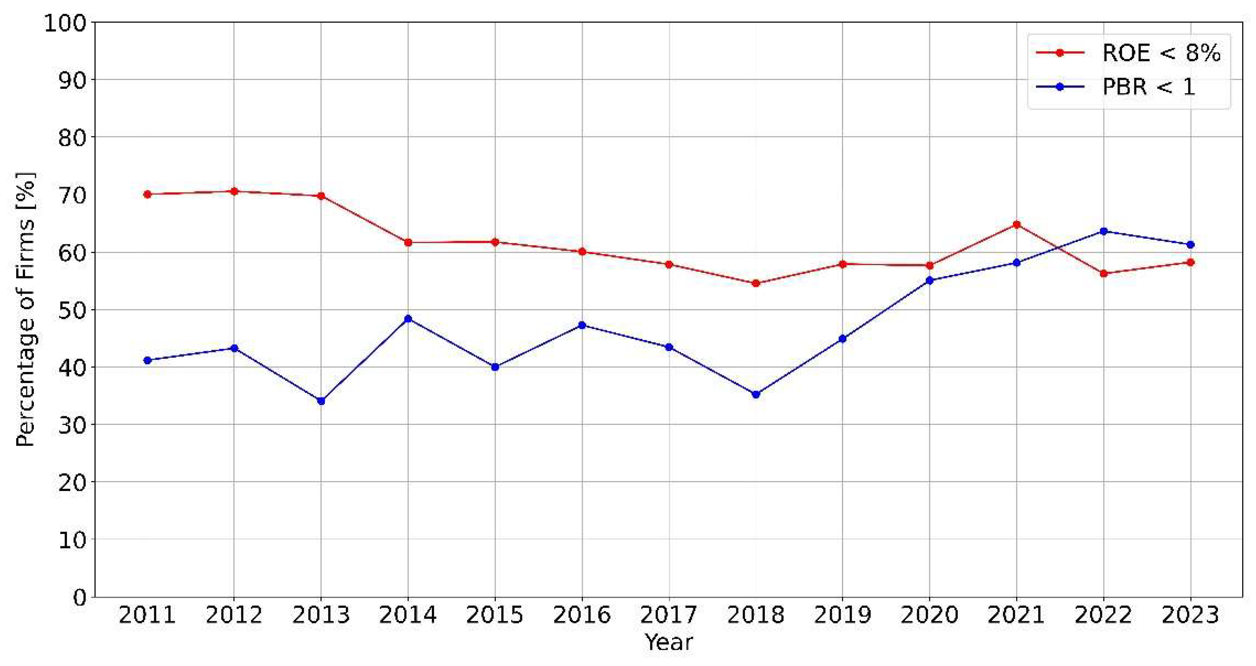
Appendix A.2. Variable-Level Relationships
For Figure A2 and Figure A3, continuous explanatory variables are divided into approximately 80 equal-width intervals after excluding observations outside the 1st–99th percentile range of each variable. Binary indicators are grouped by values of 0 and 1. Within each group, we calculate the mean variable value, observed proportion of dividend increases, and mean predicted probability. Similarly, model output is binned but without percentile trimming. These figures supplement the variable-level interpretation in Section 4.3.
Figure A2.
Relationships between explanatory variable values and observed dividend increase rates and mean predicted probabilities. Note. The blue and red points indicate the observed incidence rates and mean model predictions within groups, respectively. For variables designated as “Standardized score” in Table 4, the horizontal axis shows the mean standardized value within each interval. Percentage signs in variable names refer to their original units before standardization.
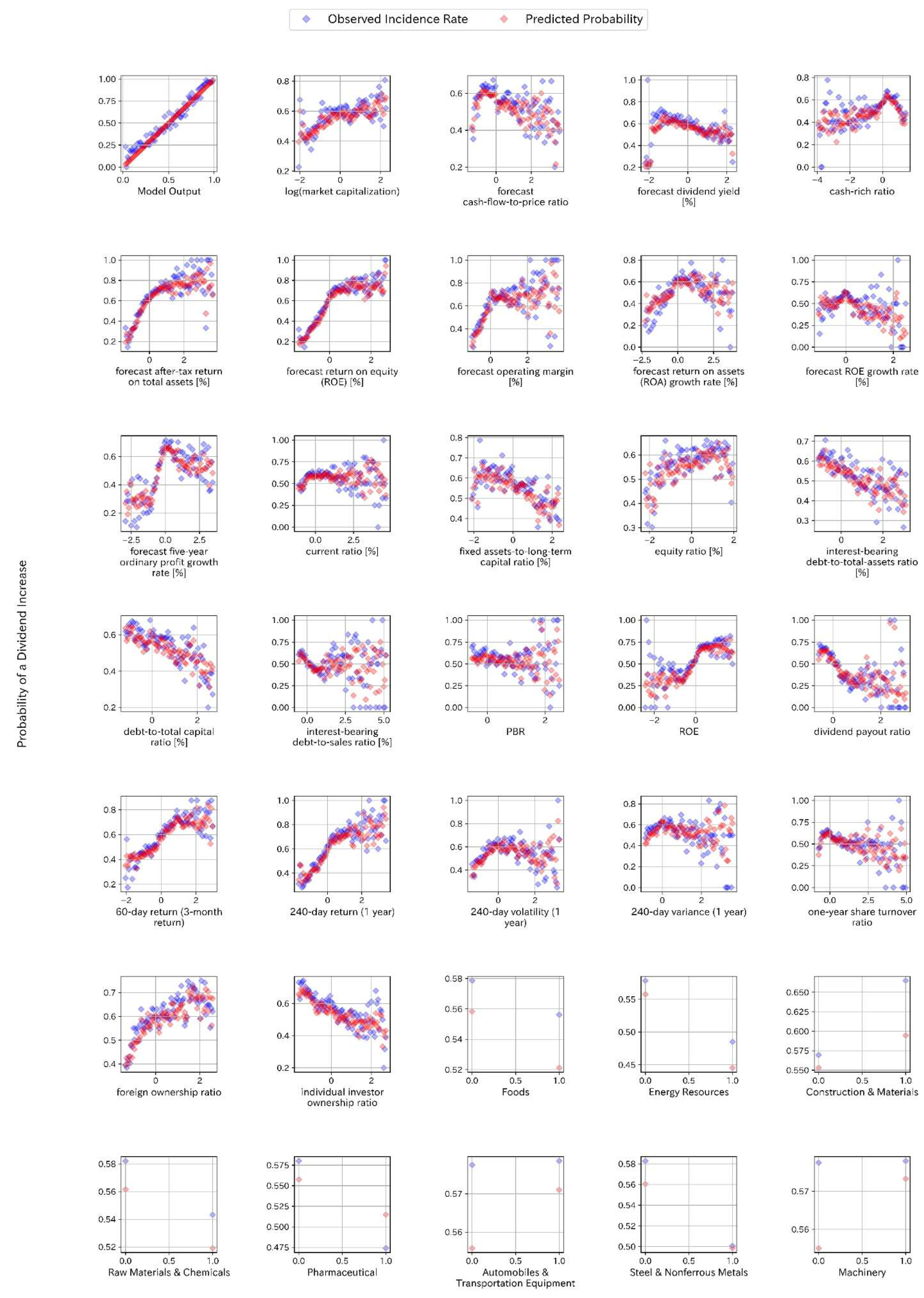
Figure A3.
Continuation of Figure A2 using the same grouping procedure and plotting conventions. Blue points indicate observed dividend-increase rates, and red points indicate mean predicted probabilities within each group.
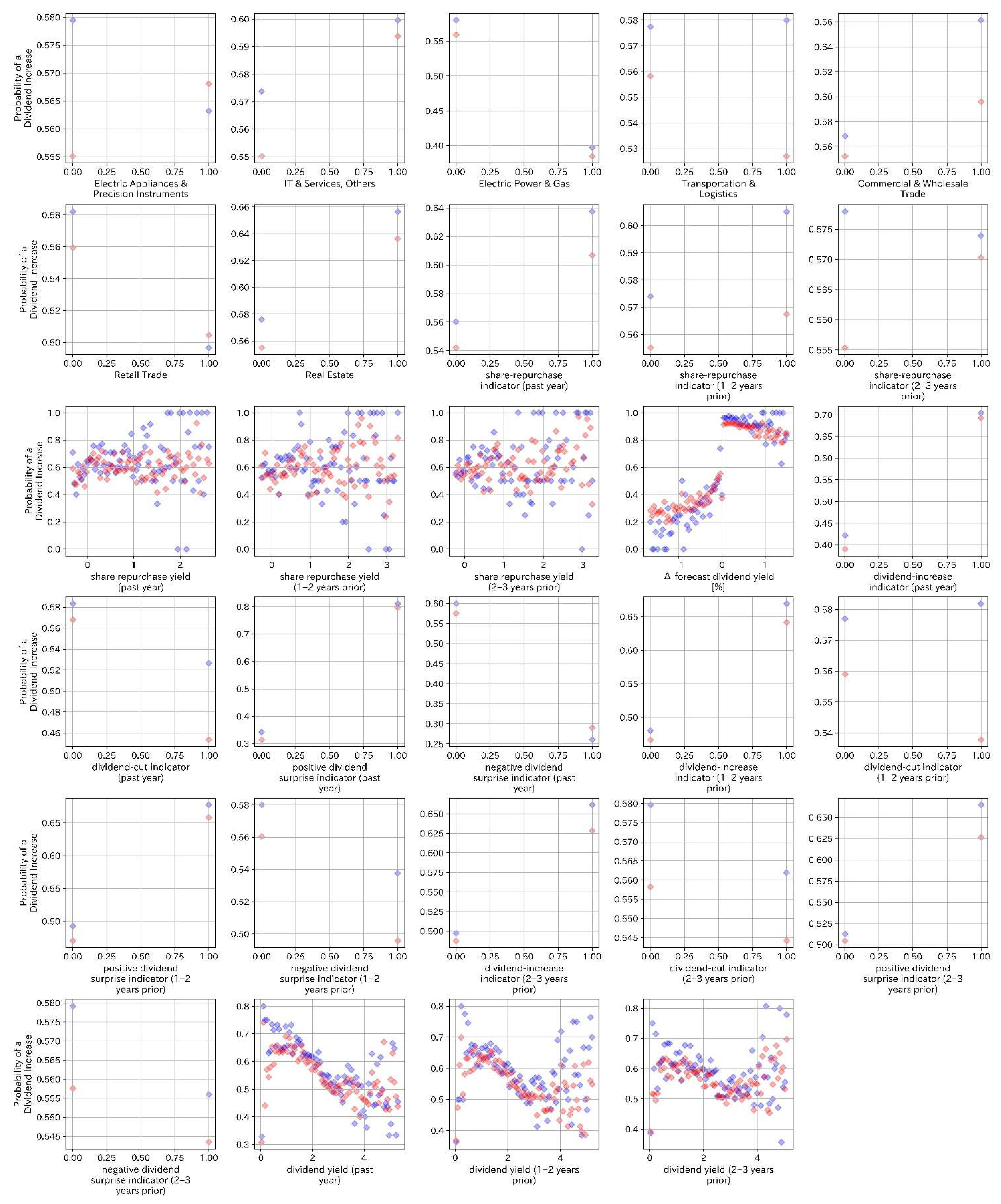
Appendix B. Annual Sample Counts and Missing Value Treatment
Appendix B.1. Annual Sample Coverage
Table A1 distinguishes the base sample from the final machine learning sample for each annual dataset from 2011 to 2023. An observation refers to a firm in one annual dataset; the total is the sum of annual observations rather than the number of distinct firms over the full period. The year designation follows Section 4.1: information available at the end of May is paired with the dividend increase outcome over the following June-to-May period.
The final machine learning sample contains 13,165 observations, including 7195 dividend increases and 5970 nonincreases. The aggregate dividend increase rate is 54.65%, calculated from the total counts. For the 2013–2023 out-of-sample datasets, the final sample comprises 11,207 observations, including 6473 dividend increases.
Table A1.
Annual sample counts, missing value exclusions, and dividend increase rates.
Appendix B.2. Missing Value Treatment
After columns not used in the model were removed, records containing a missing value in any retained data column were excluded before continuous variable standardization. No missing input values were imputed at this step. The recorded transition from the base sample to the final machine learning sample excludes seven observations: one each in 2020, 2021, and 2022, and four in 2023. These exclusions account for approximately 0.0531% of the 13,172 base observations. These counts concern this model input preparation step, not any earlier preparation of the source datasets. Missing return exclusions in Section 3.3 are handled separately for the annual return calculations.
The substantial reduction in the 2020 sample size is largely attributable to the limited availability of dividend forecasts during the COVID-19 pandemic. According to the Tokyo Stock Exchange (2020), only 52.4% of the companies covered by the report disclosed dividend forecasts as of the end of May 2020, compared with 92.8% in the previous year. Since forecast-dividend information is required for our prediction model and portfolio construction, observations lacking such information at the prediction date were excluded, contributing to the smaller sample size in 2020. Consequently, the reduced sample size also limits the coverage of the corresponding model evaluation and portfolio analysis.
Appendix C. Best Hyperparameters for Each Model by Year
Table A2 and Table A3 in this appendix present the Optuna search settings for the main hyperparameters of each machine-learning model. Table A4, Table A5, Table A6, Table A7, Table A8, Table A9, Table A10 and Table A11 report the best hyperparameters selected for each evaluation year. The best hyperparameters were selected as the combination yielding the highest validation AUC when candidate models trained on the preceding year’s data were applied to the following year’s data. The first column of each of Table A4, Table A5, Table A6, Table A7, Table A8, Table A9, Table A10 and Table A11 lists the evaluation year together with the validation AUC for that year. All random seeds used in the hyperparameter search, including random_seed and random_state, were fixed at 1234.
Table A2.
Hyperparameter search settings for k-nearest neighbors and XGBoost.
Table A3.
Hyperparameter search settings for random forest, logistic regression, and SVM.
Appendix C.1. k-Nearest Neighbors
Table A4.
Best hyperparameters for k-nearest neighbors by year.
Appendix C.2. XGBoost
Table A5.
Best hyperparameters for XGBoost by year (1).
Table A6.
Best hyperparameters for XGBoost by year (2).
Appendix C.3. Random Forest
Table A7.
Best hyperparameters for random forest by year (1).
Table A8.
Best hyperparameters for random forest by year (2).
Appendix C.4. Logistic Regression
Table A9.
Best hyperparameters for logistic regression by year.
Appendix C.5. SVM
Table A10.
Best hyperparameters for SVM by year (1).
Table A11.
Best hyperparameters for SVM by year (2).
Appendix C.6. Software and Implementation
The analysis and visualization code was written in Python 3.11. pandas and NumPy were used for tabular data processing and numerical operations, scikit-learn for preprocessing and classification metrics, XGBoost for boosted-tree models, and SHAP for model interpretation. SciPy was used for t-distribution calculations. The three-factor regression code estimates ordinary least squares coefficients with NumPy and implements the Newey–West covariance calculation in a custom function. Figures were produced with Matplotlib (version 3.10.8) and seaborn. The Optuna hyperparameter search procedure is described in Section 4.1; stored search results are read for subsequent model fitting.
Appendix D. Compounded Cumulative Return Robustness Check
This appendix provides a robustness check of the portfolio results in Section 5.1 using compounded cumulative returns. The main analysis reports arithmetic cumulative excess returns because this measure directly summarizes the monthly return differences used in the portfolio evaluation. As an additional perspective, this analysis examines how the results change when investment returns affect the value of the portfolio carried forward through time.
The analysis uses the same portfolio selections and monthly stock return inputs as Section 5.1. No model retraining or additional stock selection is introduced. Portfolios are formed once each year using the information available at the end of May, begin operation in June, and are held until the following May. At the next annual formation date, the resulting portfolio value is reallocated equally across the newly selected stocks.
Appendix D.1. Compounded Return Calculation Under Annual Rebalancing
Let p denote a portfolio, y the portfolio formation year, and m = 1, …, 12 the months from June of year y through May of year y + 1. Let denote the capital available at the beginning of formation year y, and let denote the number of stocks selected for portfolio p.
At portfolio formation, the available capital is allocated equally across the selected stocks. Therefore, the initial value assigned to stock i is as follows:
Let denote the monthly return of stock i, expressed in decimal form, using the same return inputs as in Section 5.1. During the 12-month holding period, no within-year rebalancing is performed. Instead, the value of each stock position evolves according to
Then, the month-end value of portfolio p is obtained by summing the values of all constituent positions:
As the individual positions evolve according to their own realized returns, portfolio weights are allowed to drift naturally within the holding year. Equal weights are restored only at the next annual portfolio formation.
At the end of May, the closing portfolio value becomes the capital available for the following formation year:
Thus, gains and losses are reflected continuously in portfolio value, while portfolio constituents and equal target weights are updated only once per year.
For the small number of missing monthly return observations in the selected stock matrices, the position value from the preceding month is carried forward for that month. This treatment preserves the annual holding rule and avoids mechanically reallocating capital among the remaining stocks when return availability changes.
The compounded cumulative return of portfolio p at month t is defined relative to its initial capital as
All portfolios begin with the same normalized initial capital; therefore, their compounded cumulative return paths can be directly compared.
Appendix D.2. Compounded Cumulative Return Differential (CCRD) and Benchmark Presentation
To further evaluate the stock-selection performance under compounded returns, we introduce the Compounded Cumulative Return Differential (CCRD) as a supplementary measure. This measure examines whether the performance differentiation between the top and bottom stock groups observed in the main analysis remains evident when returns are compounded over time.
TOPIX is shown as a separate market benchmark rather than being subtracted from each portfolio return. Using the same monthly TOPIX return series as in the main analysis, its normalized value evolves as
and its compounded cumulative return is 100( − 1).
For a descriptive comparison with the top-minus-bottom results in Section 5.1, CCRD is calculated as the difference between the compounded cumulative returns of the corresponding upper and lower portfolios, each formed and compounded independently as a long-only portfolio. Let and denote the normalized portfolio value factors of the top and bottom long-only portfolios for strategy s, respectively. The CCRD, expressed in percentage points, is defined as follows:
Both portfolios are financed and compounded separately as long-only portfolios. Accordingly, CCRD is a descriptive comparison and should not be interpreted as the cumulative wealth or compounded return of a self-financing long–short strategy.
Figure A4 and Figure A5 report the resulting compounded cumulative returns. Transaction costs are not deducted in these figures because the purpose of this appendix is specifically to examine the effect of compounding; turnover and transaction cost effects are evaluated separately in Section 5.3.
Appendix D.3. Results and Implications for Stock Selection
Figure A4 applies the compounded return calculation to the portfolios formed on predicted dividend increase probabilities in Figure 14.
Figure A4.
Compounded cumulative returns of portfolios formed on predicted dividend increase probabilities. Note. The lines show compounded cumulative returns for the top, middle, and bottom predicted-probability terciles, perfect foresight, and TOPIX. The pink bars indicate CCRD (Compounded Cumulative Return Differential), defined as the difference between the compounded cumulative returns of the separately financed top and bottom long-only portfolios, expressed in percentage points. Perfect foresight is an ex post, nontradable reference.
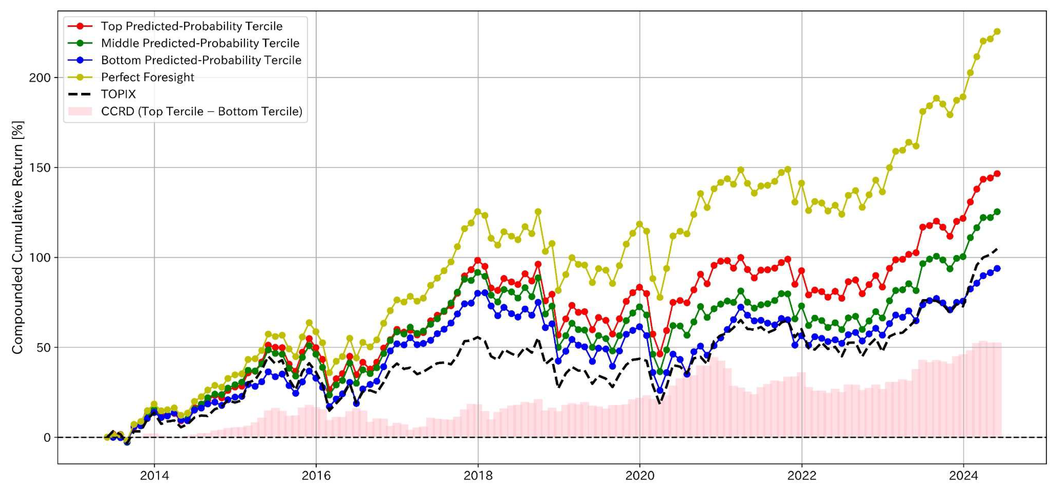
The probability-sorted portfolios retain the broad performance ordering observed in Figure 14. At the end of the evaluation period, the compounded cumulative returns are 225.58% for perfect foresight, 146.53% for the top predicted-probability tercile, 125.38% for the middle tercile, and 93.88% for the bottom tercile. TOPIX records a compounded cumulative return of 104.73%. Thus, the top portfolio finishes above the market benchmark, whereas the bottom portfolio finishes below it. The terminal CCRD between the top and bottom long-only portfolios is 52.65 percentage points.
These results indicate that the predicted probability of a dividend increase continues to distinguish stocks with stronger and weaker subsequent performance when returns are compounded through the holding period. Therefore, the robustness check supports the stock selection interpretation of the prediction signal reported in Section 5.1.
Figure A5.
Comparison of compounded cumulative portfolio performance across the three investment strategies. Note. Panels (a–c) show the compounded cumulative returns of the corresponding upper and lower stock groups together with TOPIX. The pink bars show CCRD, the compounded cumulative return differential between separately financed top and bottom long-only portfolios. Panel (d) compares CCRD across the three strategies on the same scale.
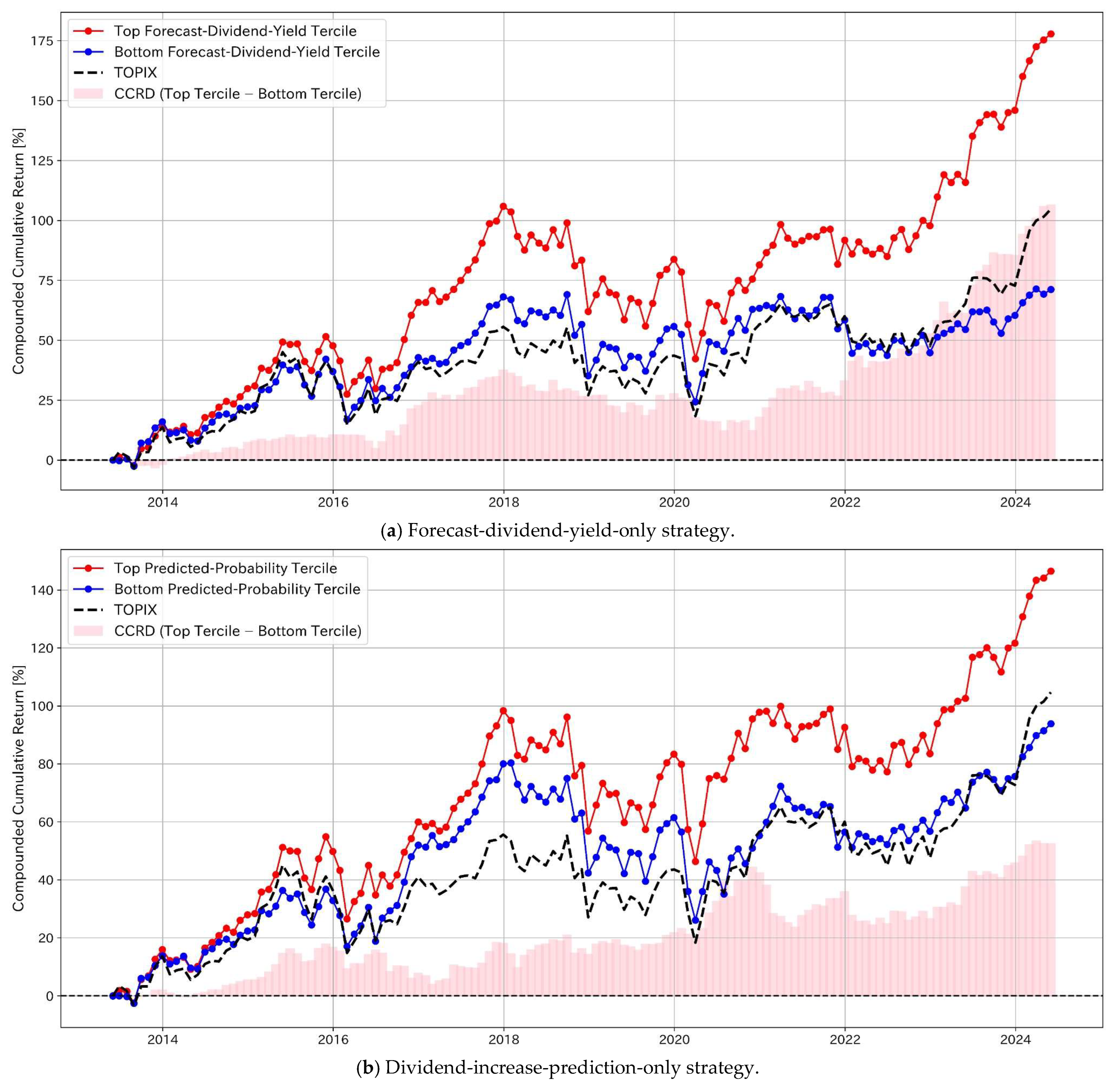
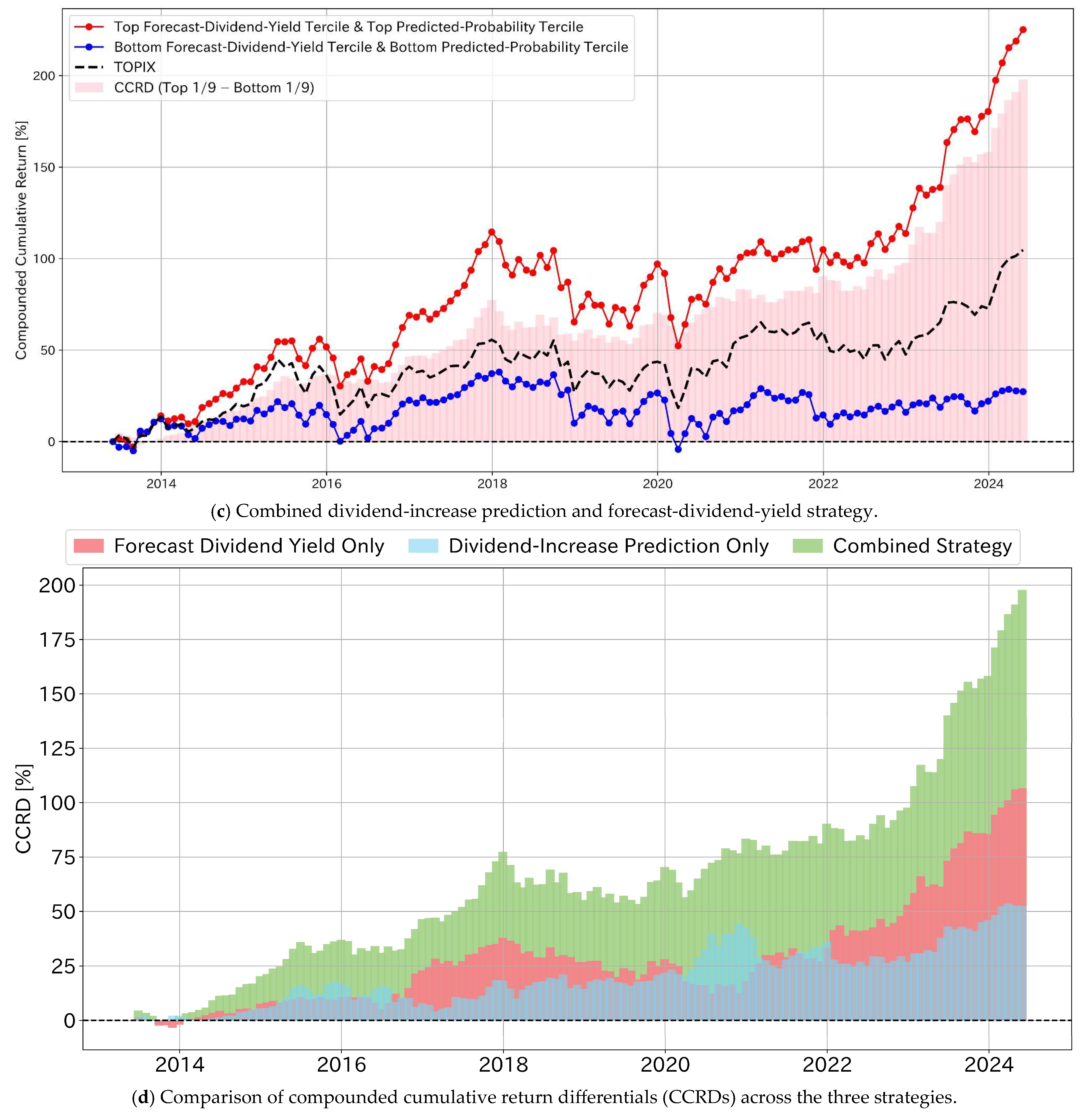
The terminal CCRD values are 106.64, 52.65, and 197.85 percentage points for the forecast-dividend-yield-only, dividend-increase-prediction-only, and combined strategies, respectively. Therefore, the combined strategy exhibits the largest CCRD among the three approaches. These values describe differences between independent long-only portfolios and are not compounded returns from self-financing long–short investment accounts.
This ordering is consistent with the main results in Figure 16. Therefore, the additional compounded return analysis does not alter the principal stock-selection conclusion: combining the predicted probability of a dividend increase with forecast dividend yield provides stronger stock selection performance than using either signal alone. Moreover, the result supports the interpretation that forecast dividend yield and predicted dividend increase probability provide complementary information on the current level of dividend income and prospect of future dividend growth.
References
- Akindayomi, A., & Amin, M. R. (2022). Does business strategy affect dividend payout policies? Journal of Business Research, 151, 531–550. [Google Scholar] [CrossRef] [Scilit]
- Anolick, N., Batten, J. A., Kinateder, H., & Wagner, N. (2021). Time for gift giving: Abnormal share repurchase returns and uncertainty. Journal of Corporate Finance, 66, 101787. [Google Scholar] [CrossRef] [Scilit]
- Arena, M. P., & Julio, B. (2023). Litigation risk management through corporate payout policy. Journal of Financial and Quantitative Analysis, 58(1), 148–174. [Google Scholar] [CrossRef] [Scilit]
- Bhattacharya, S. (1979). Imperfect information, dividend policy, and “the bird in the hand” fallacy. The Bell Journal of Economics, 10(1), 259–270. [Google Scholar] [CrossRef] [Scilit]
- Bourveau, T., Li, X., Macciocchi, D., & Sun, C. (2023). Mutual funds’ reporting frequency and firms’ responses to undervaluation: The role of share repurchases. Contemporary Accounting Research, 40(4), 2616–2642. [Google Scholar] [CrossRef] [Scilit]
- Chang, H., Ishida, S., & Kochiyama, T. (2024). Management forecasting ability and predictive ability of dividend changes for future earnings. Journal of Accounting, Auditing & Finance, 39(1), 304–331. [Google Scholar] [CrossRef] [Scilit]
- DeAngelo, H., DeAngelo, L., & Stulz, R. M. (2006). Dividend policy and the earned/contributed capital mix: A test of the life-cycle theory. Journal of Financial Economics, 81(2), 227–254. [Google Scholar] [CrossRef] [Scilit]
- Easterbrook, F. H. (1984). Two agency-cost explanations of dividends. The American Economic Review, 74(4), 650–659. [Google Scholar]
- French, K. R. (2025). Fama/French Japanese 3 factors. Kenneth R. French Data Library. Available online: https://mba.tuck.dartmouth.edu/pages/faculty/ken.french/data_library.html (accessed on 25 July 2025).
- Grullon, G., Michaely, R., & Swaminathan, B. (2002). Are dividend changes a sign of firm maturity? The Journal of Business, 75(3), 387–424. [Google Scholar] [CrossRef] [Scilit] [PubMed]
- Gu, S., Kelly, B. T., & Xiu, D. (2020). Empirical asset pricing via machine learning. The Review of Financial Studies, 33(5), 2223–2273. [Google Scholar] [CrossRef] [Scilit]
- Ikenberry, D., Lakonishok, J., & Vermaelen, T. (1995). Market underreaction to open market share repurchases. Journal of Financial Economics, 39(2–3), 181–208. [Google Scholar] [CrossRef] [Scilit]
- Jagannathan, M., Stephens, C. P., & Weisbach, M. S. (2000). Financial flexibility and the choice between dividends and stock repurchases. Journal of Financial Economics, 57(3), 355–384. [Google Scholar] [CrossRef] [Scilit]
- Jensen, M. C. (1986). Agency costs of free cash flow, corporate finance, and takeovers. The American Economic Review, 76(2), 323–329. [Google Scholar]
- Julio, B., & Ikenberry, D. L. (2004). Reappearing dividends. Journal of Applied Corporate Finance, 16(4), 89–100. [Google Scholar] [CrossRef] [Scilit]
- Katsafados, A. G., Leledakis, G. N., Panagiotou, N. P., & Pyrgiotakis, E. G. (2026). Can central bankers’ talk predict bank stock returns? A machine learning approach. International Review of Financial Analysis, 119, 105465. [Google Scholar] [CrossRef] [Scilit]
- Kim, J.-B., Luo, L., & Xie, H. (2024). Do dividends mitigate bad news hoarding, overinvestments, and stock price crash risk? Accounting & Finance, 64(4), 3999–4038. [Google Scholar] [CrossRef] [Scilit]
- Kitamura, T., & Kojima, S. (2019). Effects of changes in ownership structure on the management of regional banks. Securities Analysts Journal, 57(4), 67–78. [Google Scholar]
- Lin, J.-C., & Yu, M.-T. (2025). Managerial overconfidence and dividend stickiness. Journal of Accounting, Auditing & Finance, 40(1), 165–192. [Google Scholar] [CrossRef] [Scilit]
- Lintner, J. (1956). Distribution of incomes of corporations among dividends, retained earnings, and taxes. The American Economic Review, 46(2), 97–113. [Google Scholar]
- Lo, A. W. (2004). The adaptive markets hypothesis: Market efficiency from an evolutionary perspective. The Journal of Portfolio Management, 30(5), 15–29. [Google Scholar] [CrossRef] [Scilit]
- Michaely, R., Thaler, R. H., & Womack, K. L. (1995). Price reactions to dividend initiations and omissions: Overreaction or drift? The Journal of Finance, 50(2), 573–608. [Google Scholar] [CrossRef]
- Michałowski, M. (2025). Market reactions to dividend increases and cuts: A decade-long event study analysis of the Warsaw stock exchange. Financial Sciences. Nauki o Finansach, 30(1), 35–45. [Google Scholar] [CrossRef] [Scilit]
- Miller, M. H., & Rock, K. (1985). Dividend policy under asymmetric information. The Journal of Finance, 40(4), 1031–1051. [Google Scholar] [CrossRef]
- Mochizuki, K., Tamura, S., Kakara, T., & Suzuki, T. (2026). Predicting share repurchases based on corporate financial indicators using machine learning and examining their potential applications. JAFEE Journal, 24, 58–78. (In Japanese) [Google Scholar] [CrossRef] [PubMed]
- Mohanram, P., Saiy, S., & Vyas, D. (2018). Fundamental analysis of banks: The use of financial statement information to screen winners from losers. Review of Accounting Studies, 23(1), 200–233. [Google Scholar] [CrossRef] [Scilit]
- Myers, S. C., & Majluf, N. S. (1984). Corporate financing and investment decisions when firms have information that investors do not have. Journal of Financial Economics, 13(2), 187–221. [Google Scholar] [CrossRef] [Scilit]
- Tokyo Stock Exchange. (2020). 2020年3月期決算発表状況の集計結果について [Summary of financial results announcements for the fiscal year ended march 2020]. Available online: https://www.jpx.co.jp/news/1023/nlsgeu000004rbjm-att/nlsgeu000004rbm7.pdf (accessed on 30 October 2026).
- Tokyo Stock Exchange. (2023). Action to implement management that is conscious of cost of capital and stock price. Available online: https://www.jpx.co.jp/english/news/1020/dreu250000004n19-att/dreu250000004n8s.pdf (accessed on 5 November 2026).
- Uchiyama, T., & Takahashi, H. (2015). Information content of dividend increase and share buyback. In JSAI technical report (Vol. BI-003, pp. 1–6). Type 2 SIG. (In Japanese). [Google Scholar] [CrossRef] [PubMed]
- Ueno, Y., & Baba, N. (2005). Determinants of shareholder payout policies among Japanese firms: An empirical analysis of incentives for dividends and cancellation of treasury shares [Bank of Japan Working Paper Series, 05-J-6]. Available online: https://www.boj.or.jp/research/wps_rev/wps_2005/wp05j06.htm (accessed on 1 September 2026).
- Vermaelen, T. (1981). Common stock repurchases and market signalling: An empirical study. Journal of Financial Economics, 9(2), 139–183. [Google Scholar] [CrossRef] [Scilit]
- Wu, X. (2020). Event-driven learning of systematic behaviours in stock markets. arXiv, arXiv:2010.15586. [Google Scholar] [CrossRef] [Scilit]
- Yamamoto, R., Kawadai, N., & Kurita, M. (2020). Examining the applicability of earnings-release and shikiho text information to investment strategies. JAFEE Journal, 18, 46–62. (In Japanese) [Google Scholar] [CrossRef] [PubMed]
- Ye, Z. J., & Schuller, B. W. (2020). Capturing dynamics of post-earnings-announcement drift using genetic algorithm-optimised supervised learning. arXiv, arXiv:2009.03094. [Google Scholar] [CrossRef] [Scilit]
- Zurek, M., & Heinrich, L. (2021). Bottom-up versus top-down factor investing: An alpha forecasting perspective. Journal of Asset Management, 22(1), 11–29. [Google Scholar] [CrossRef] [Scilit]
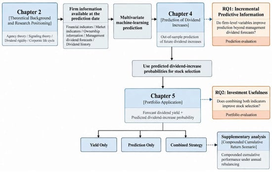
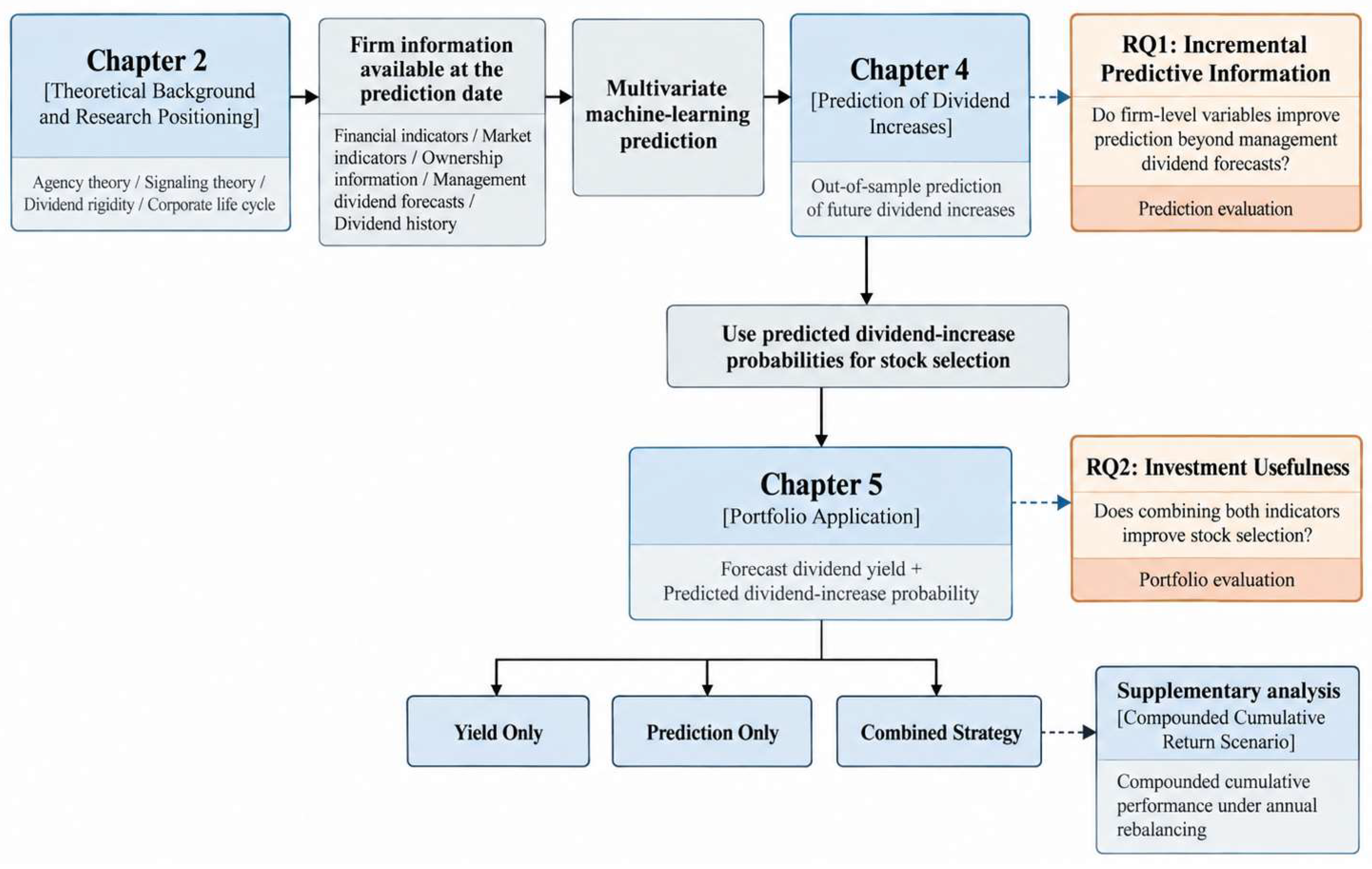
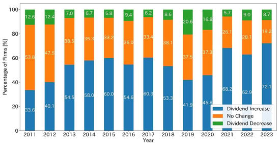
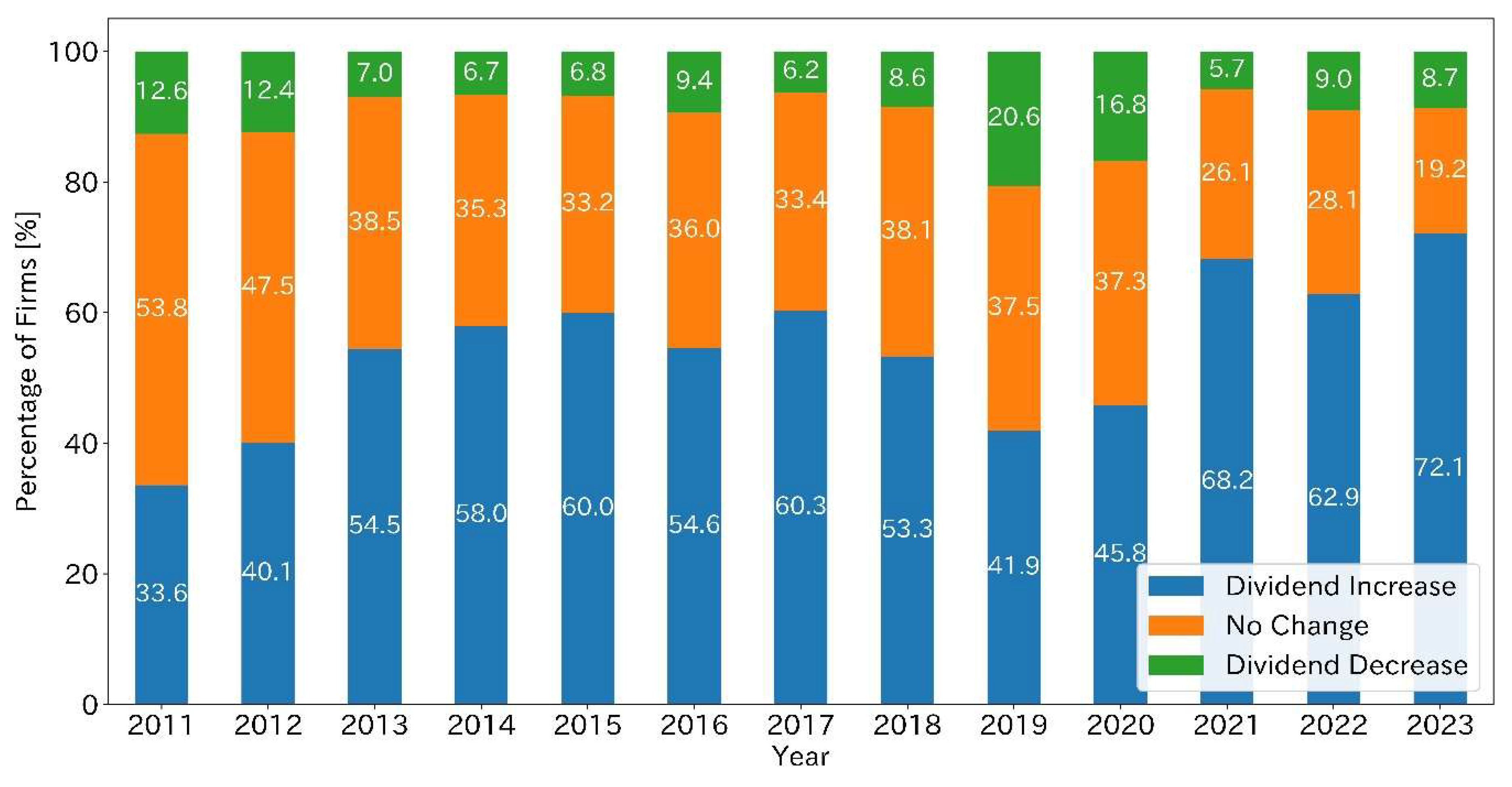
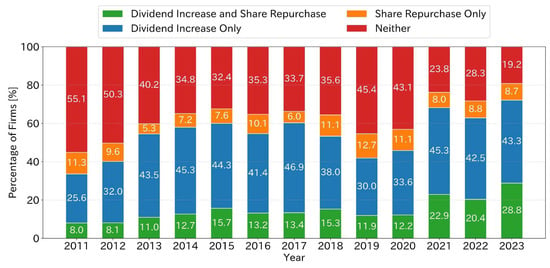
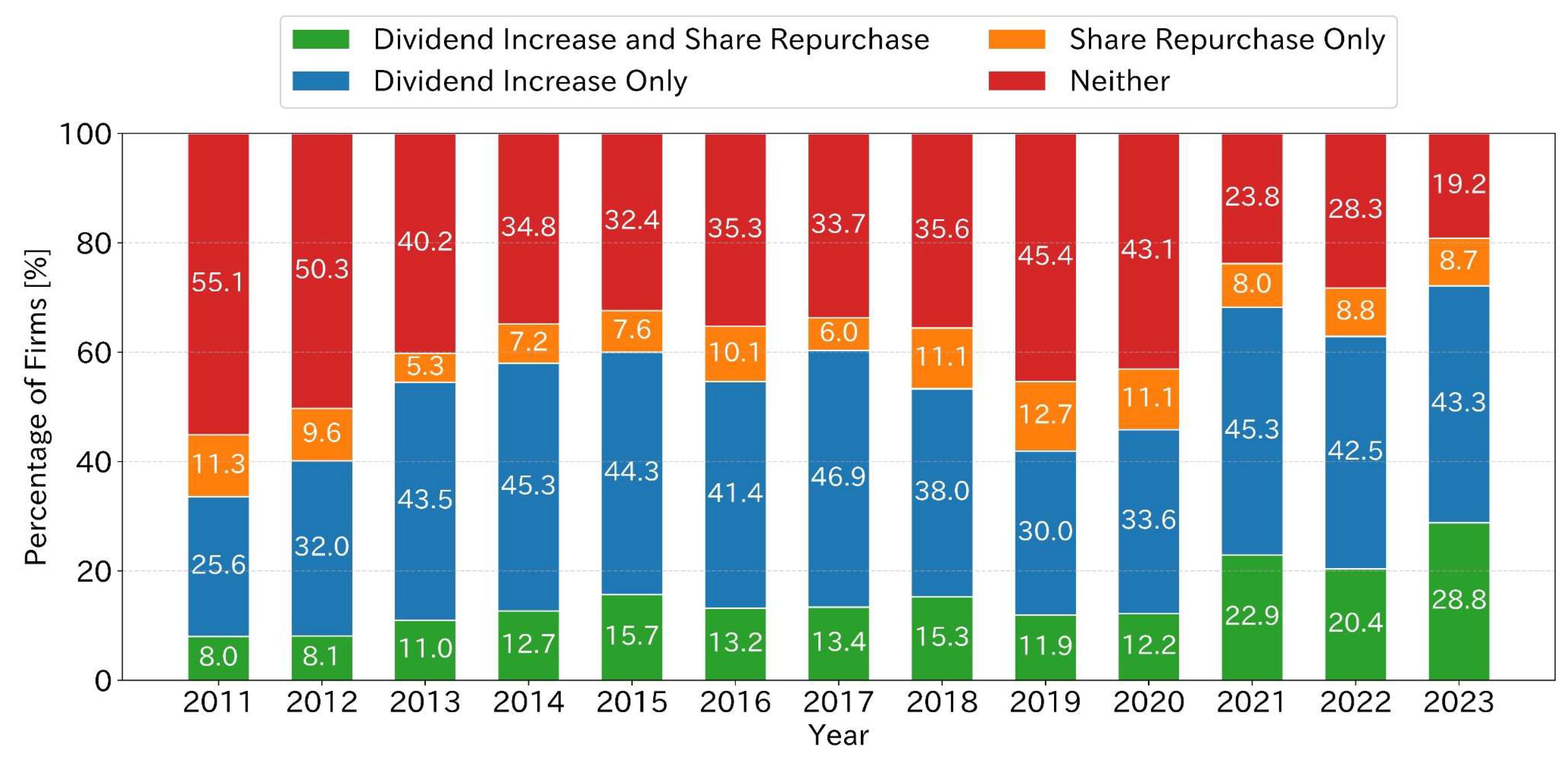
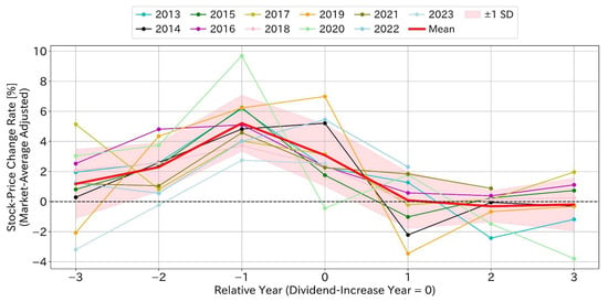
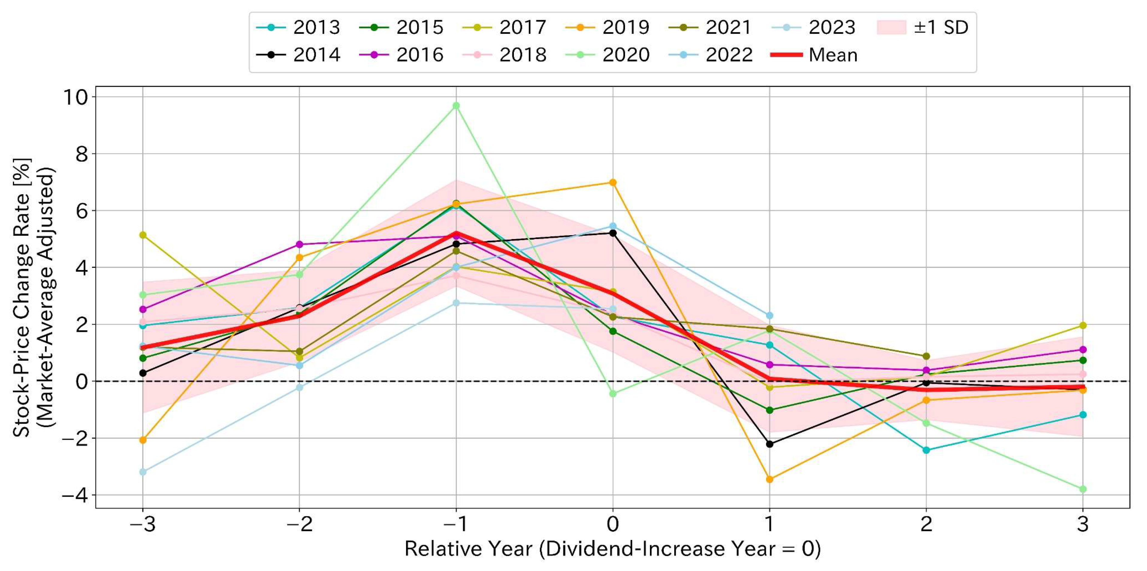
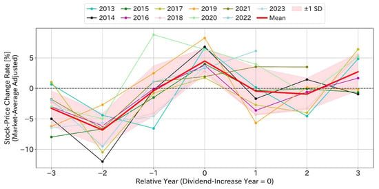
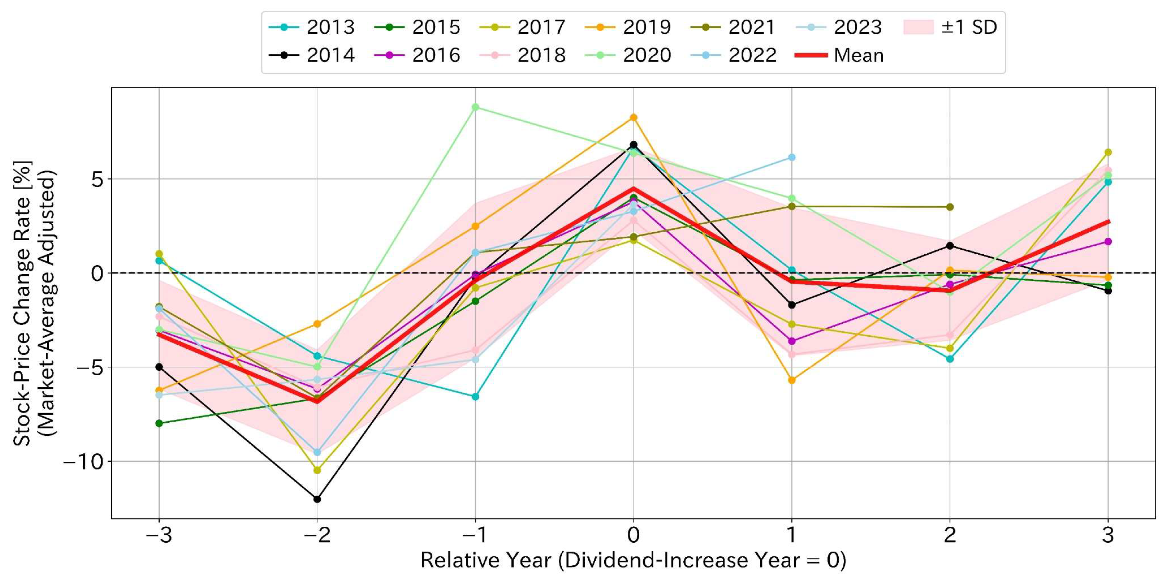
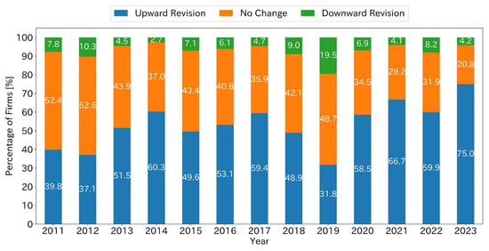
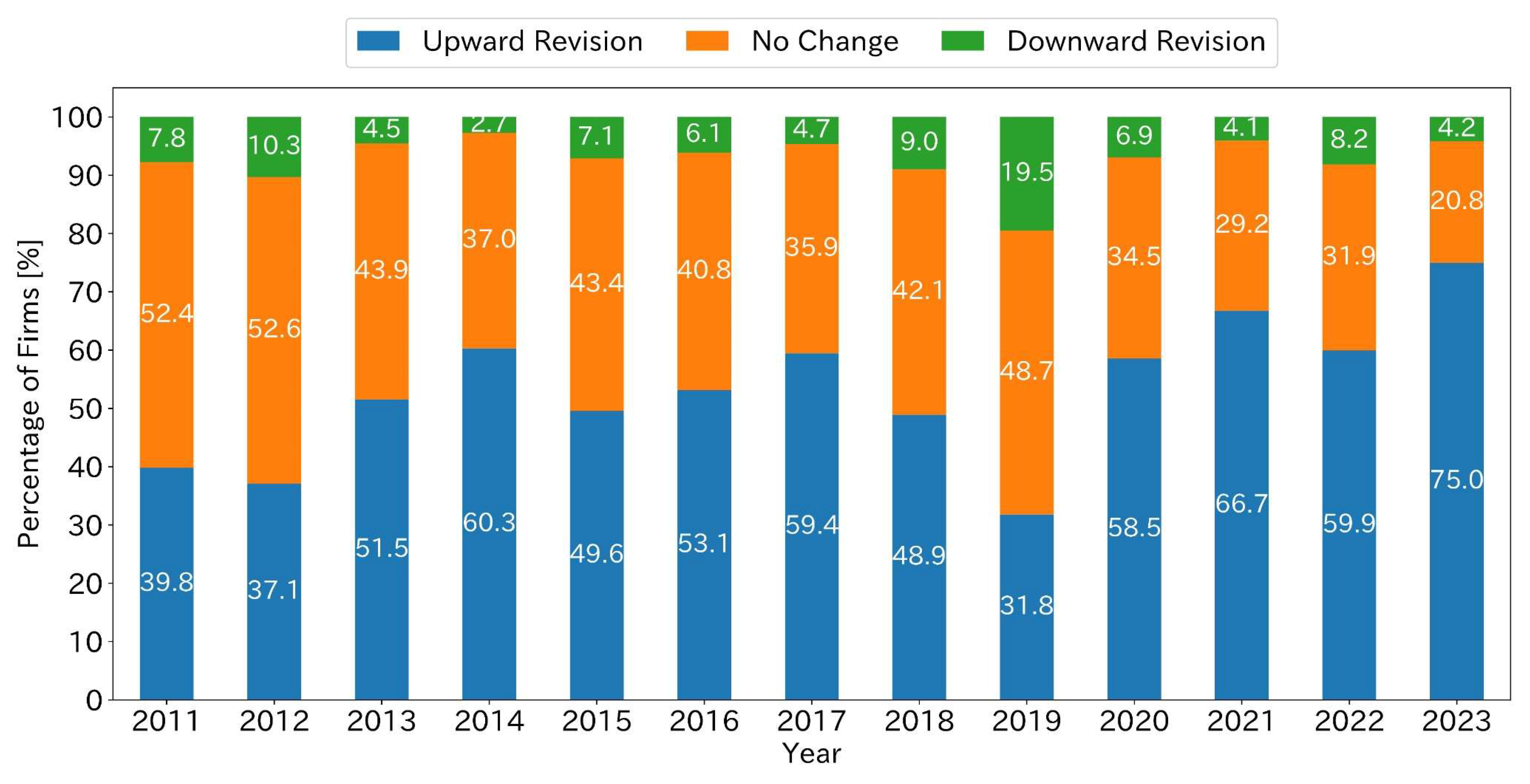
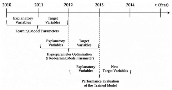
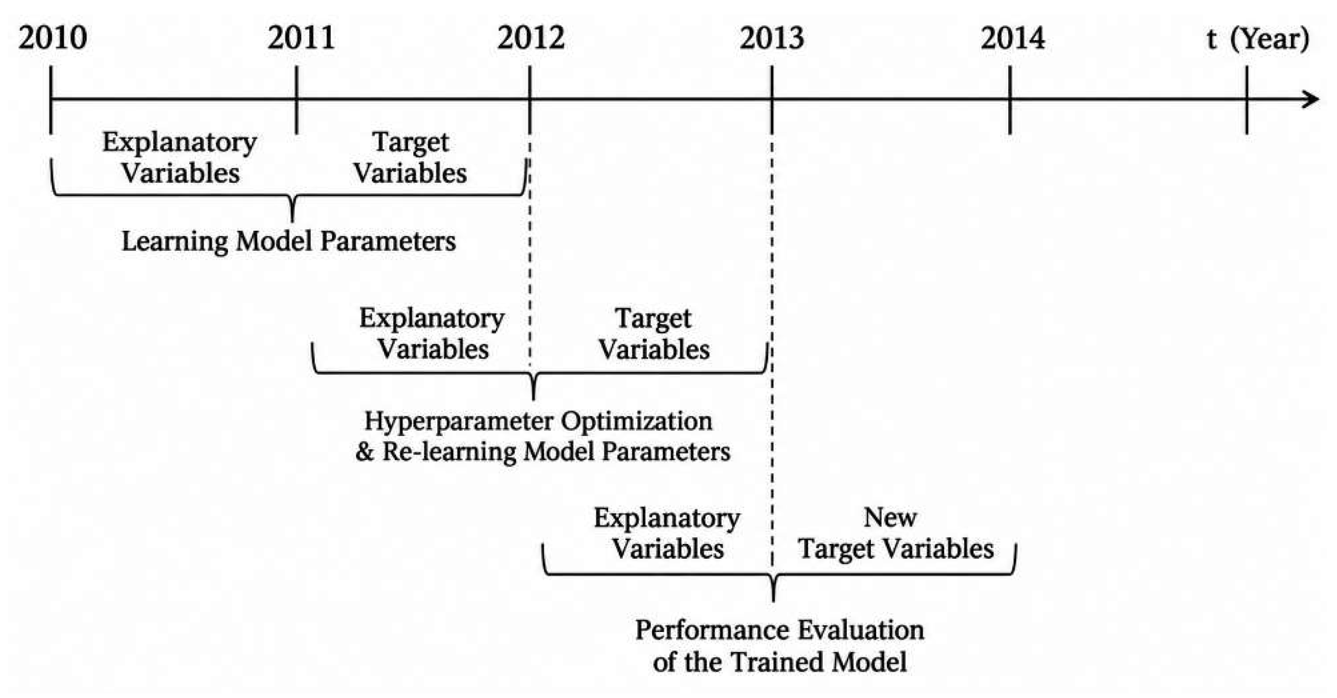
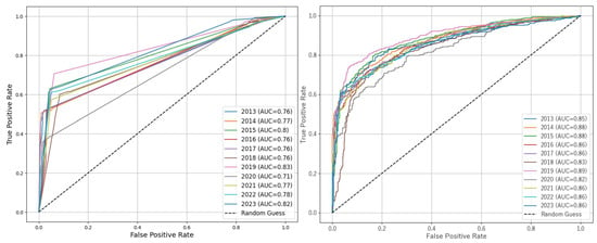
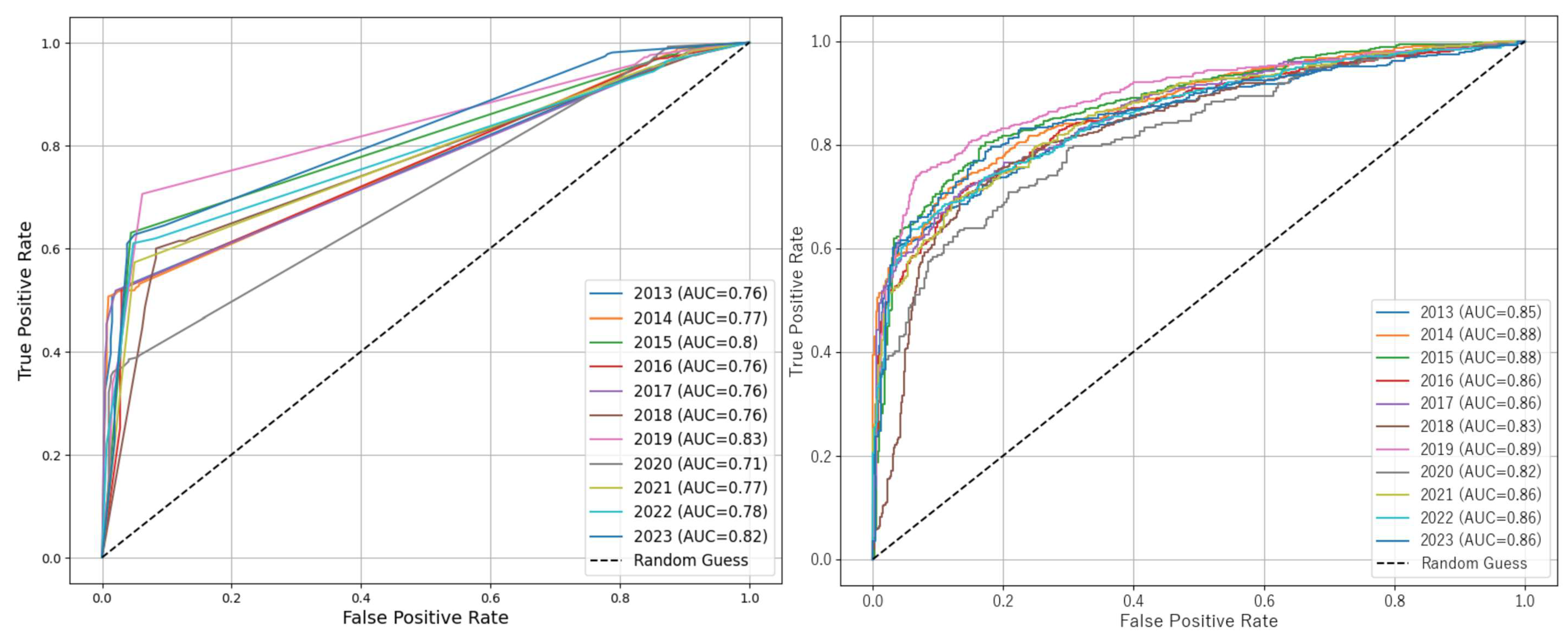
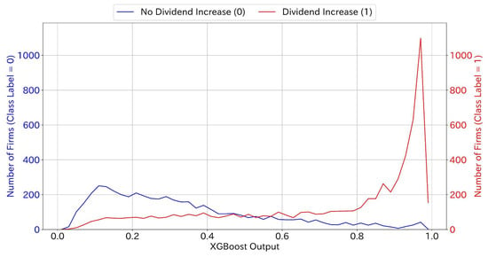
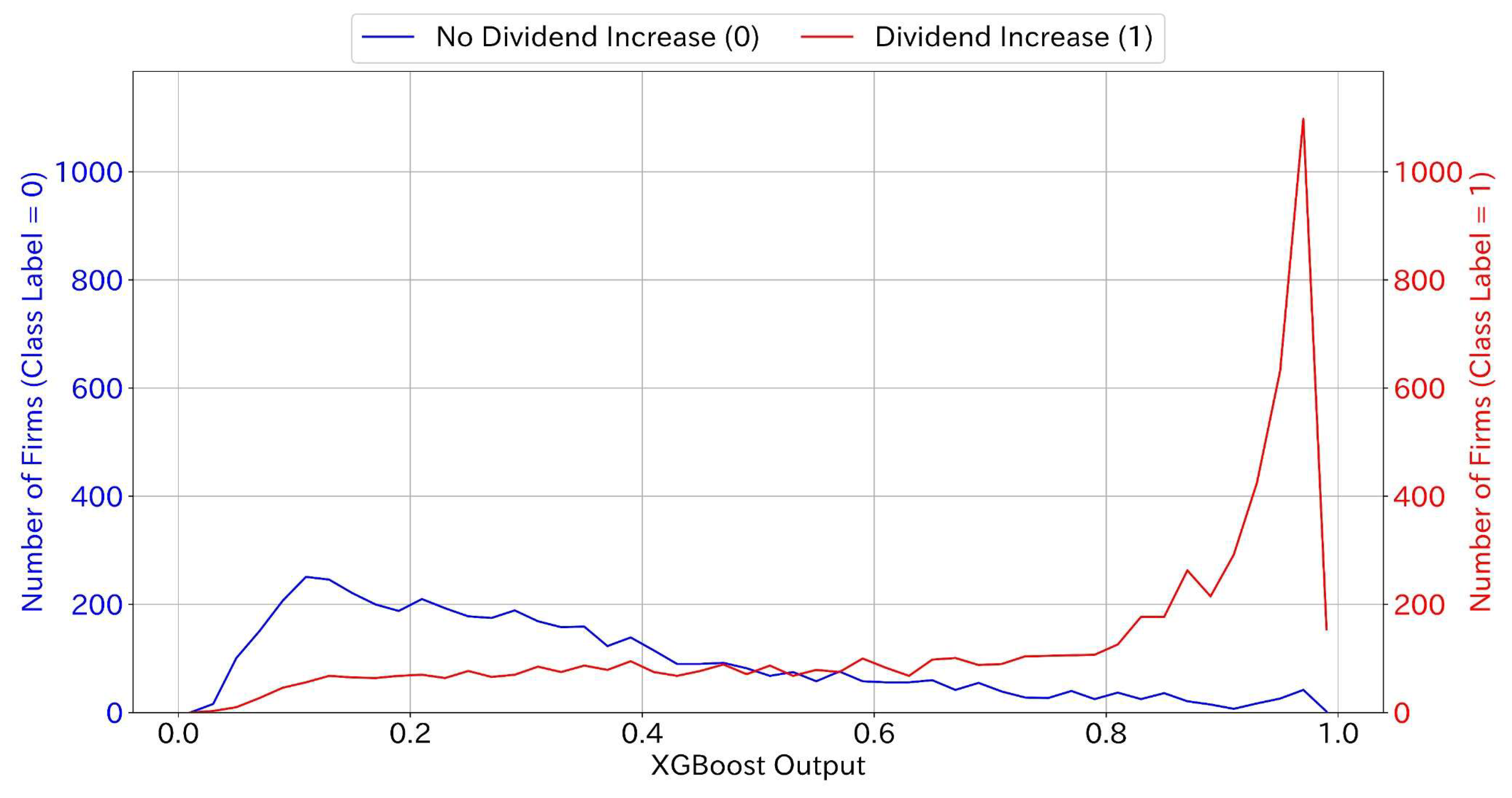
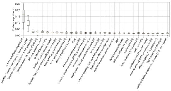
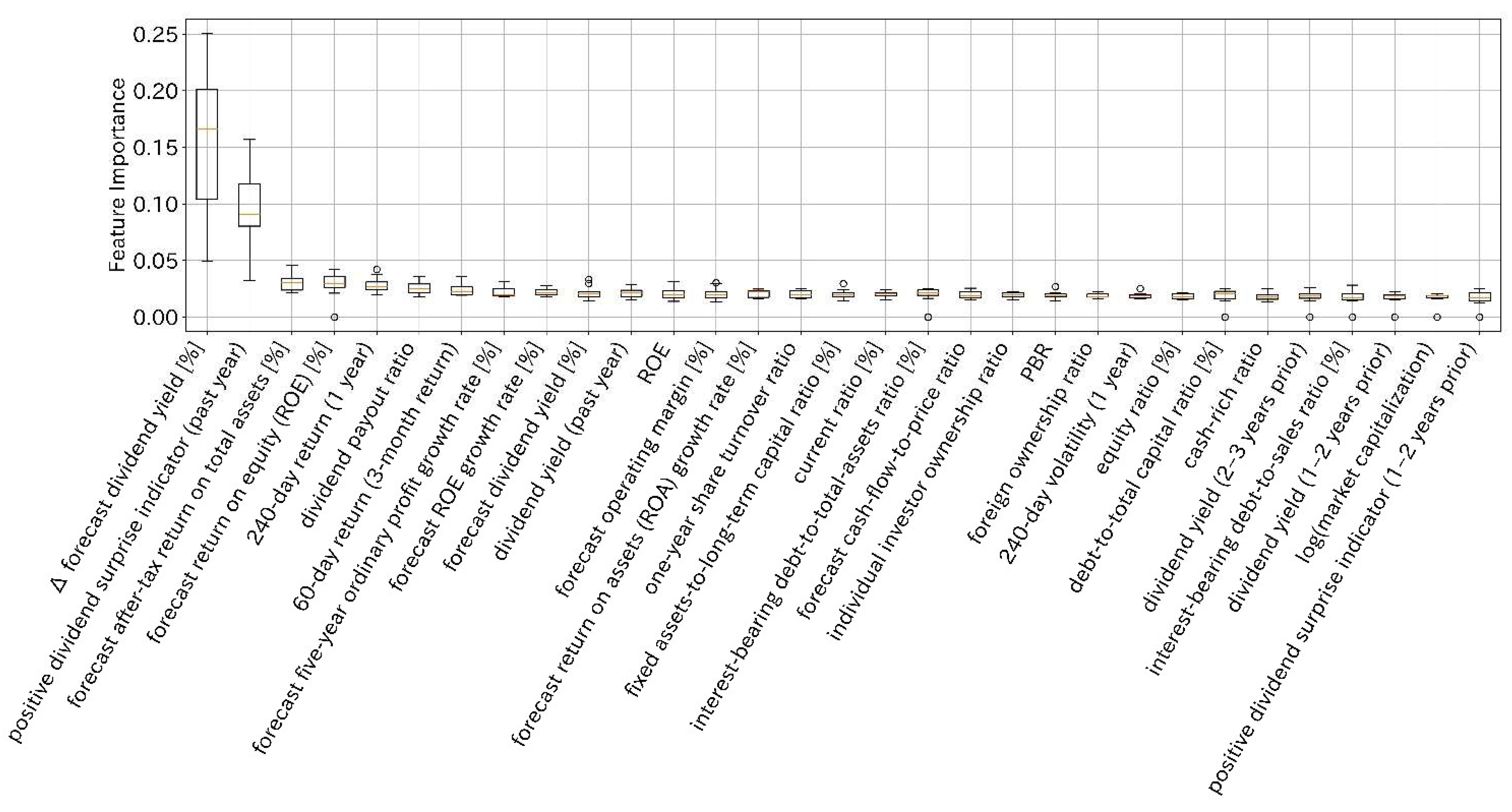
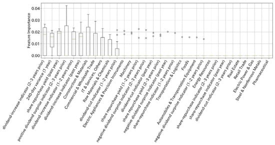
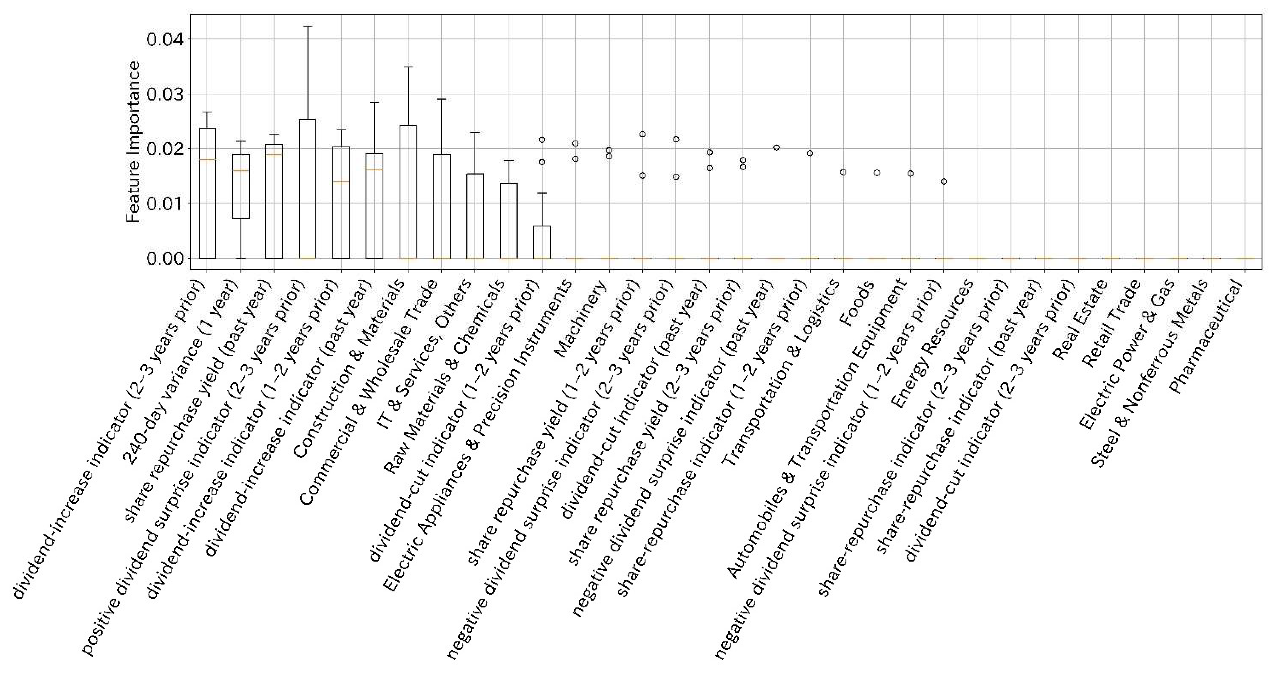
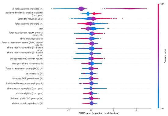
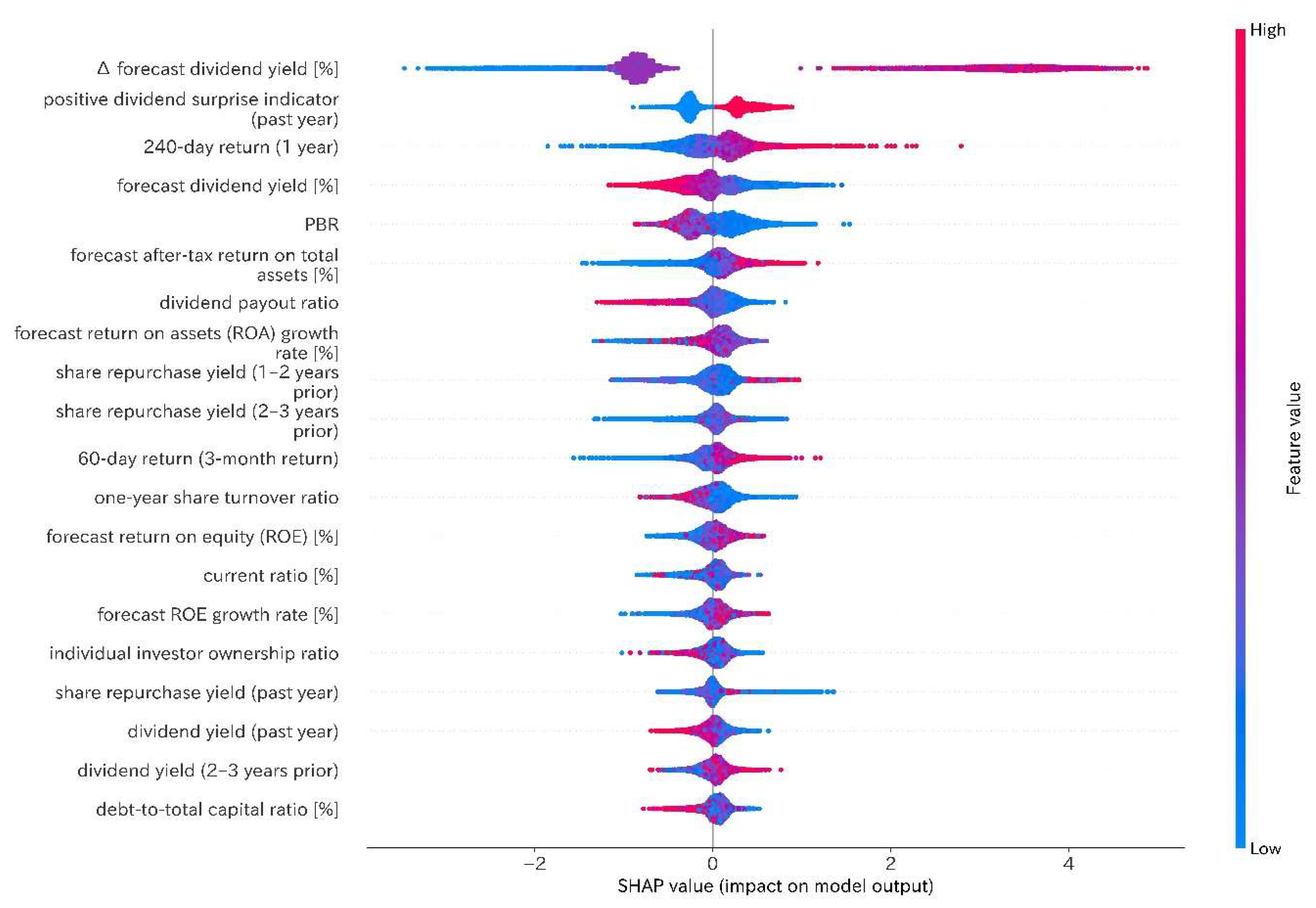
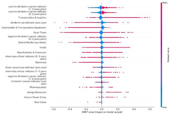
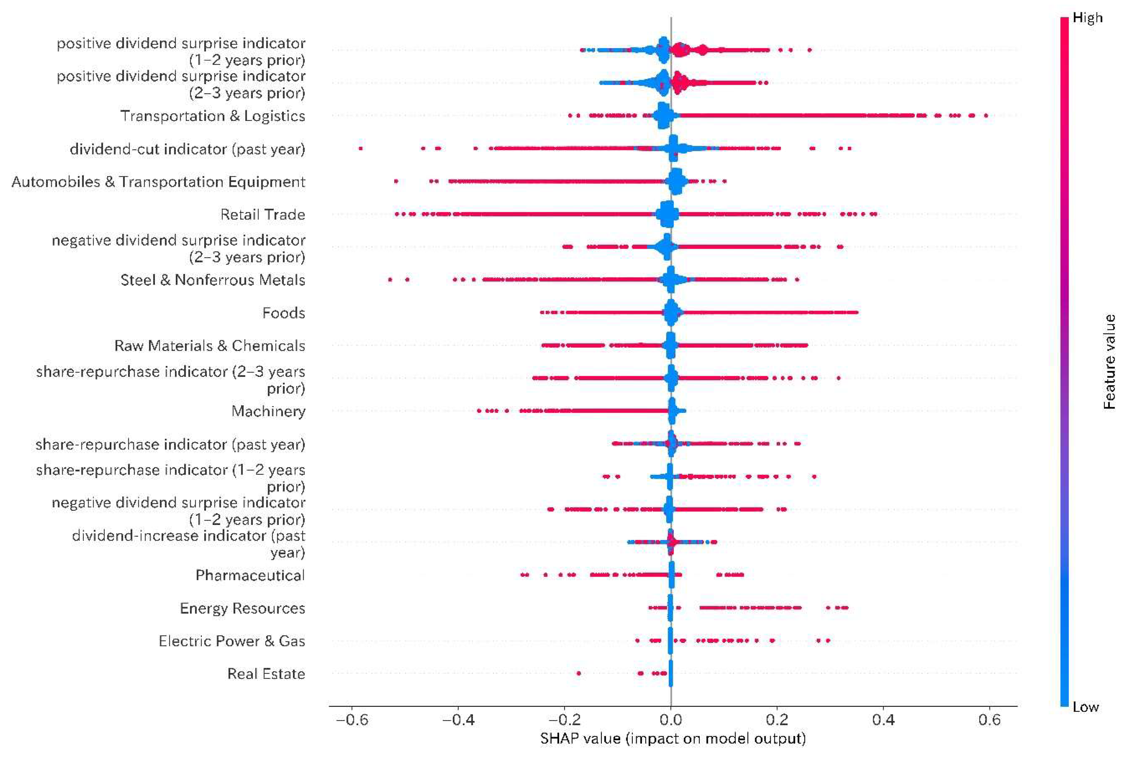
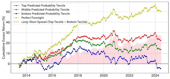
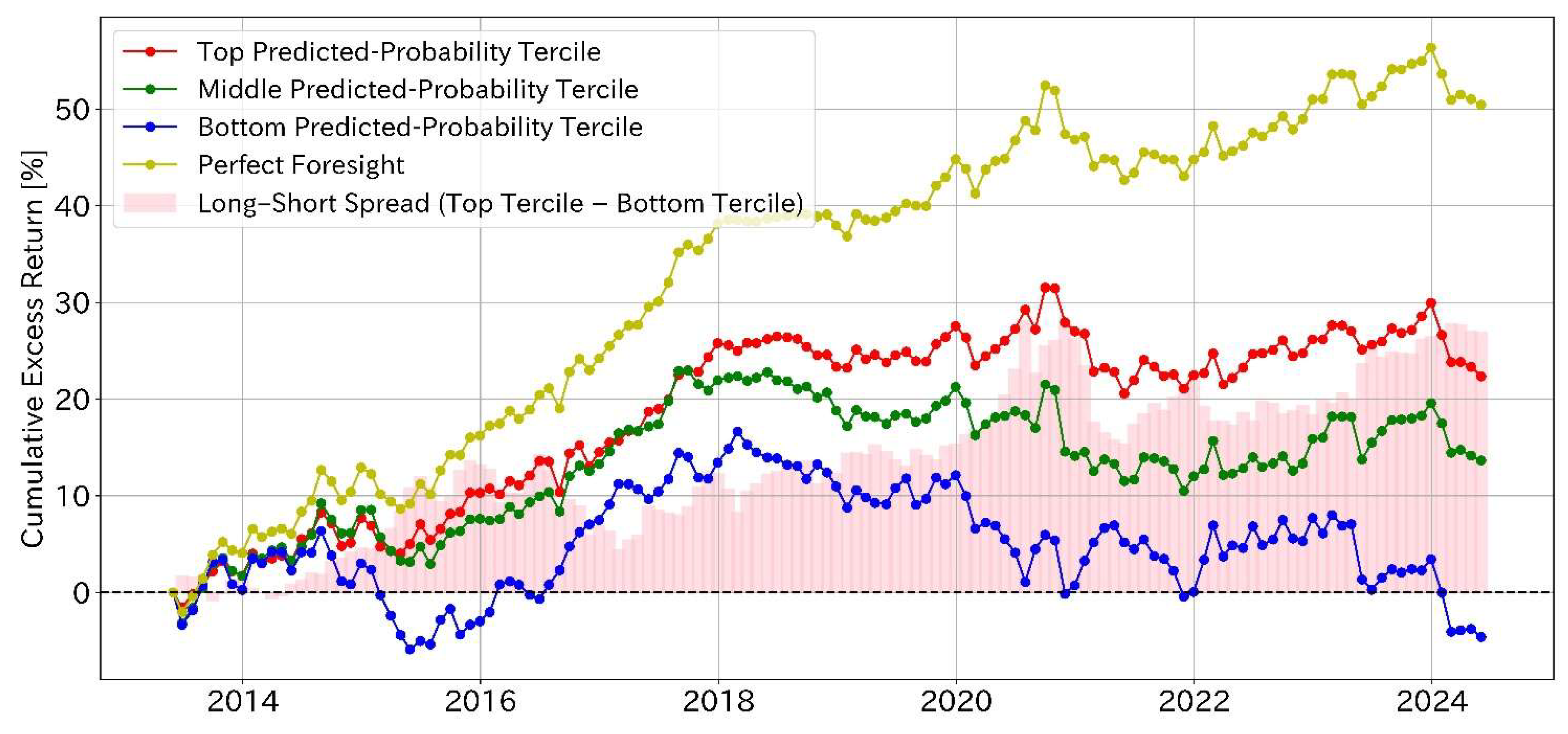
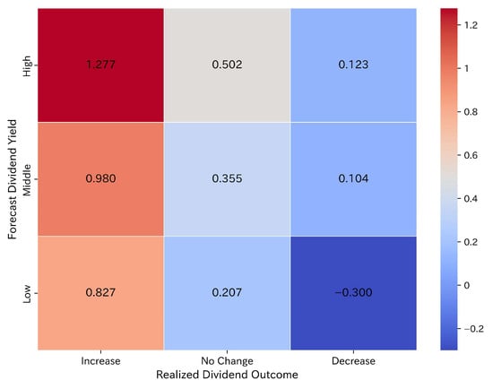
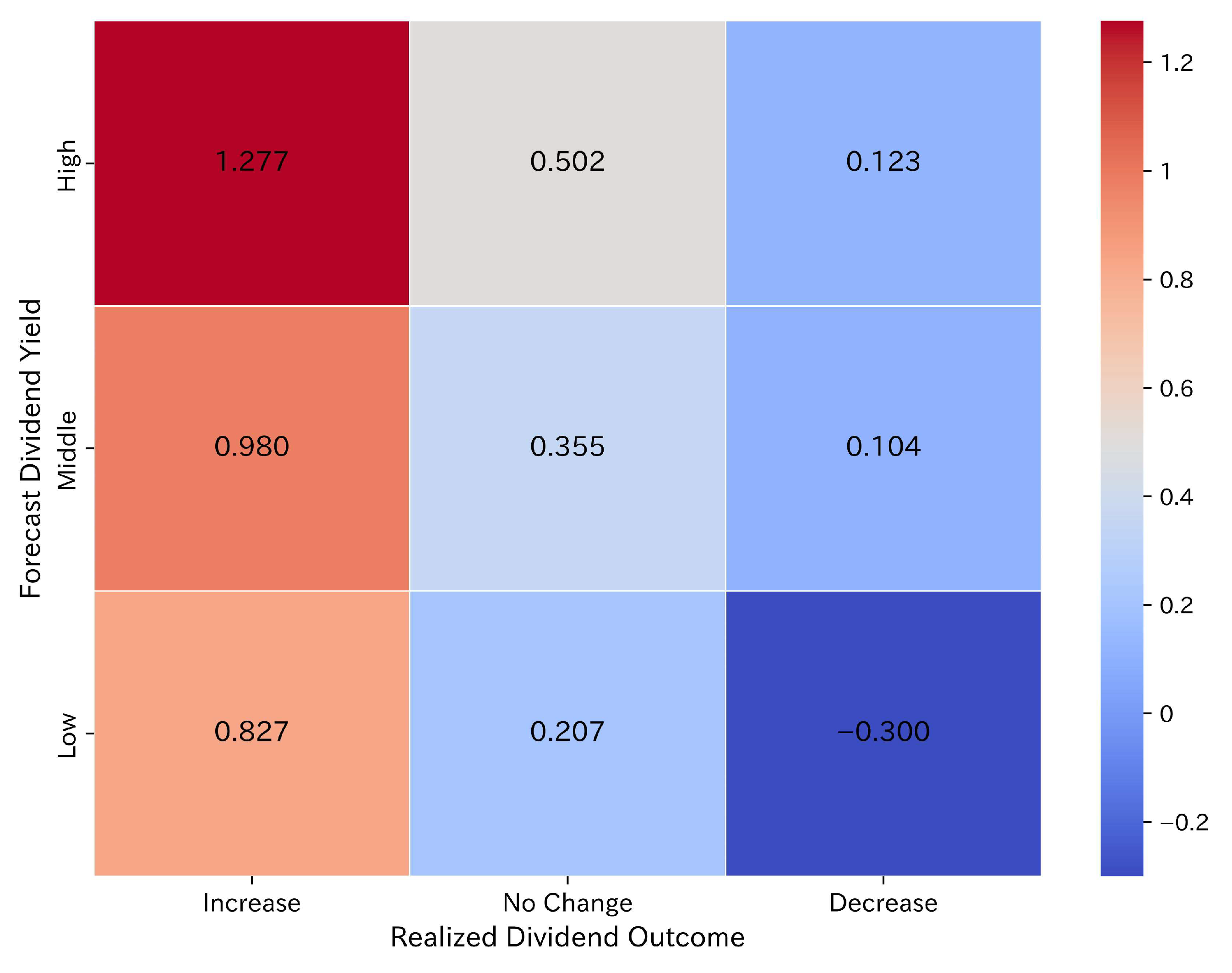
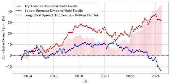
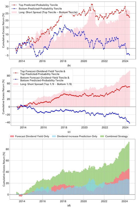
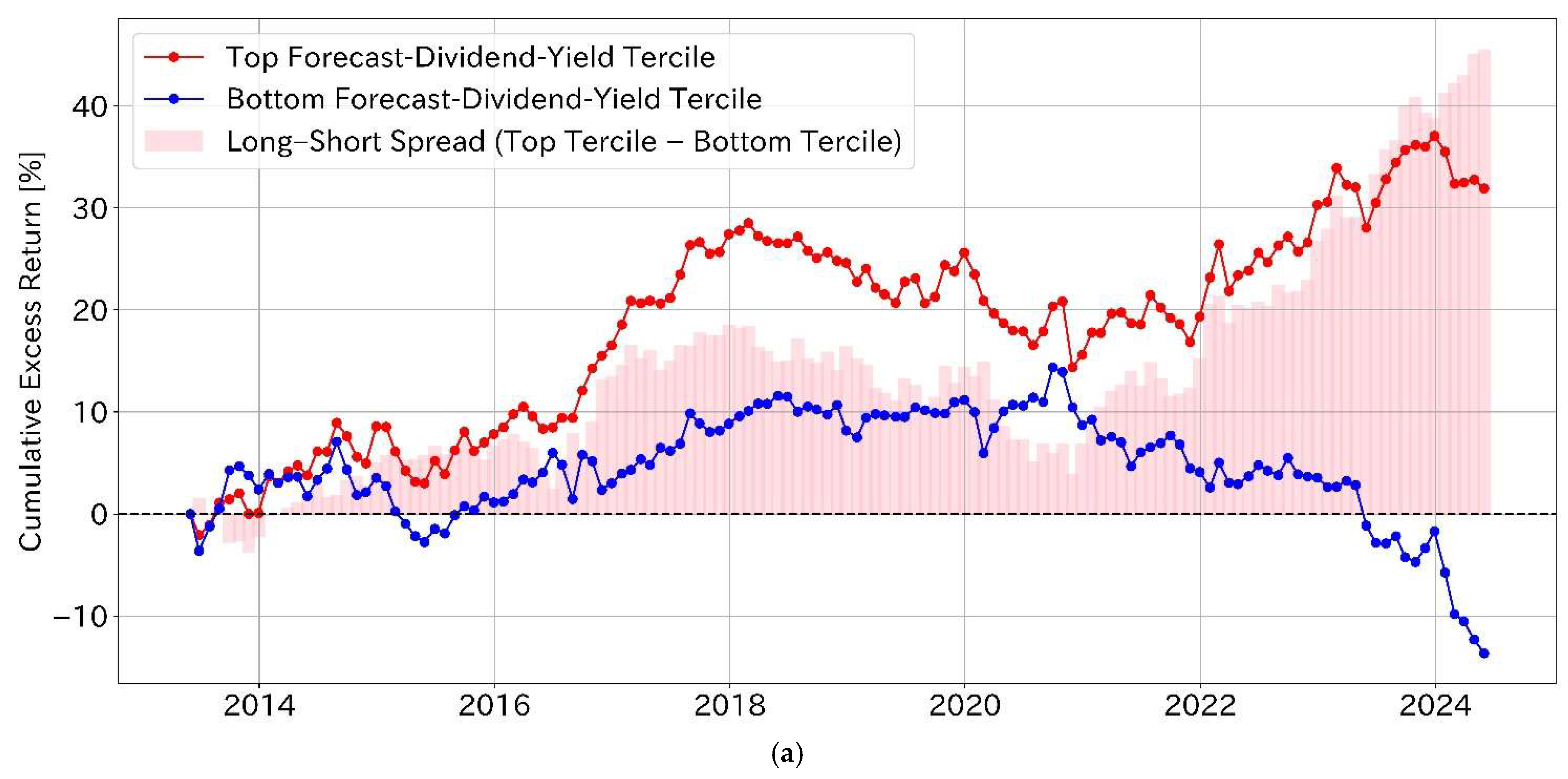
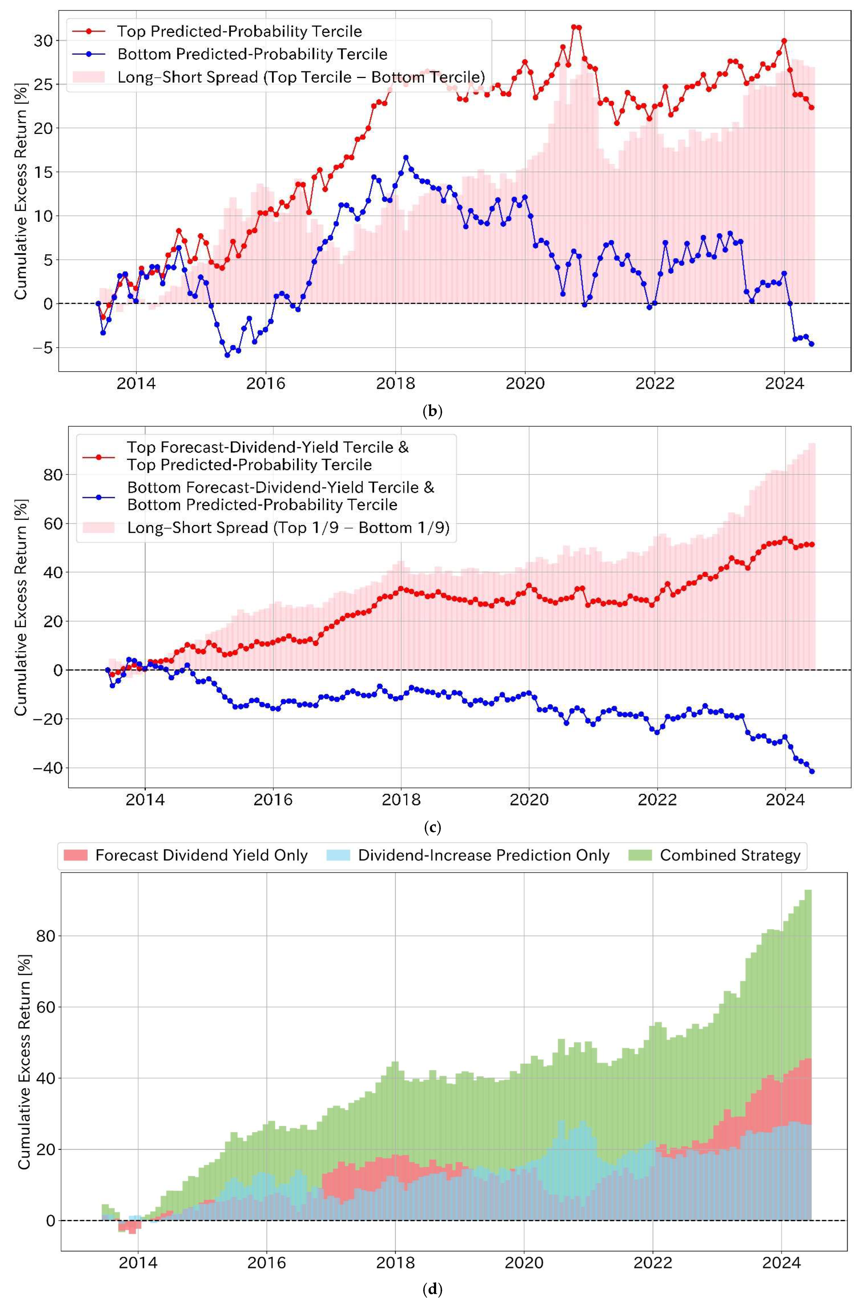
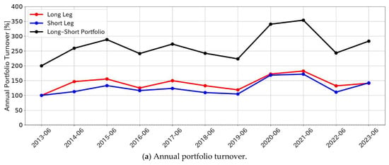
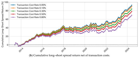
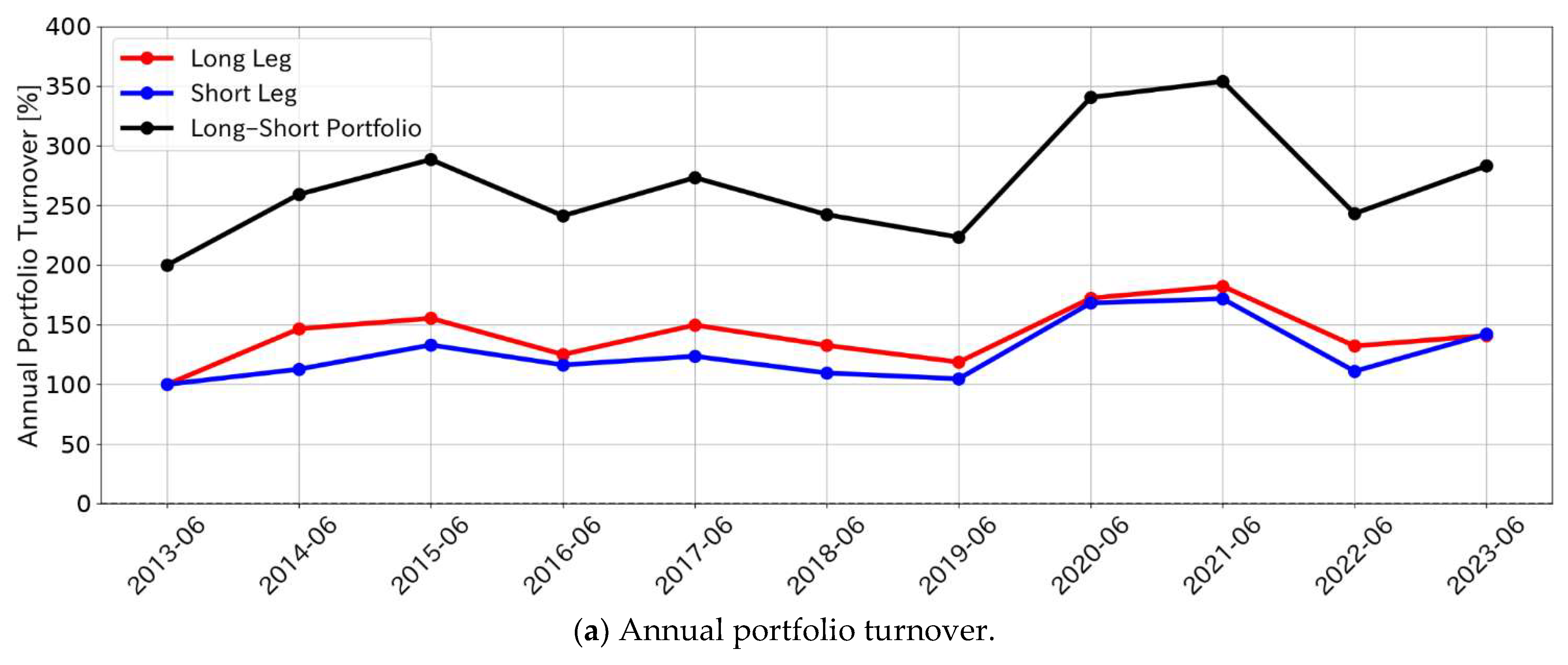
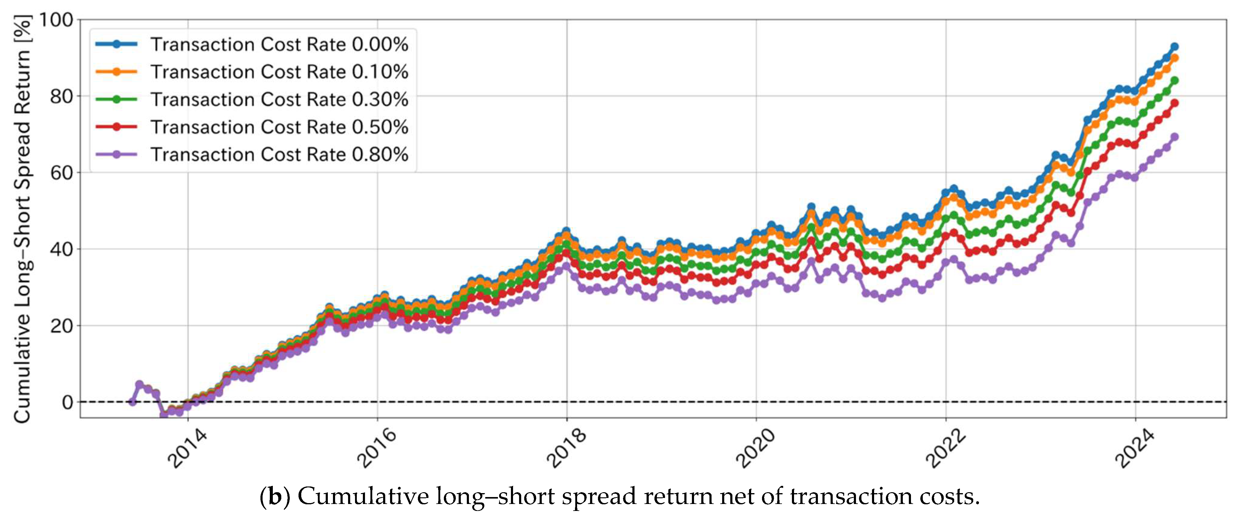
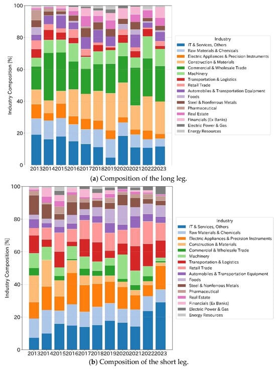
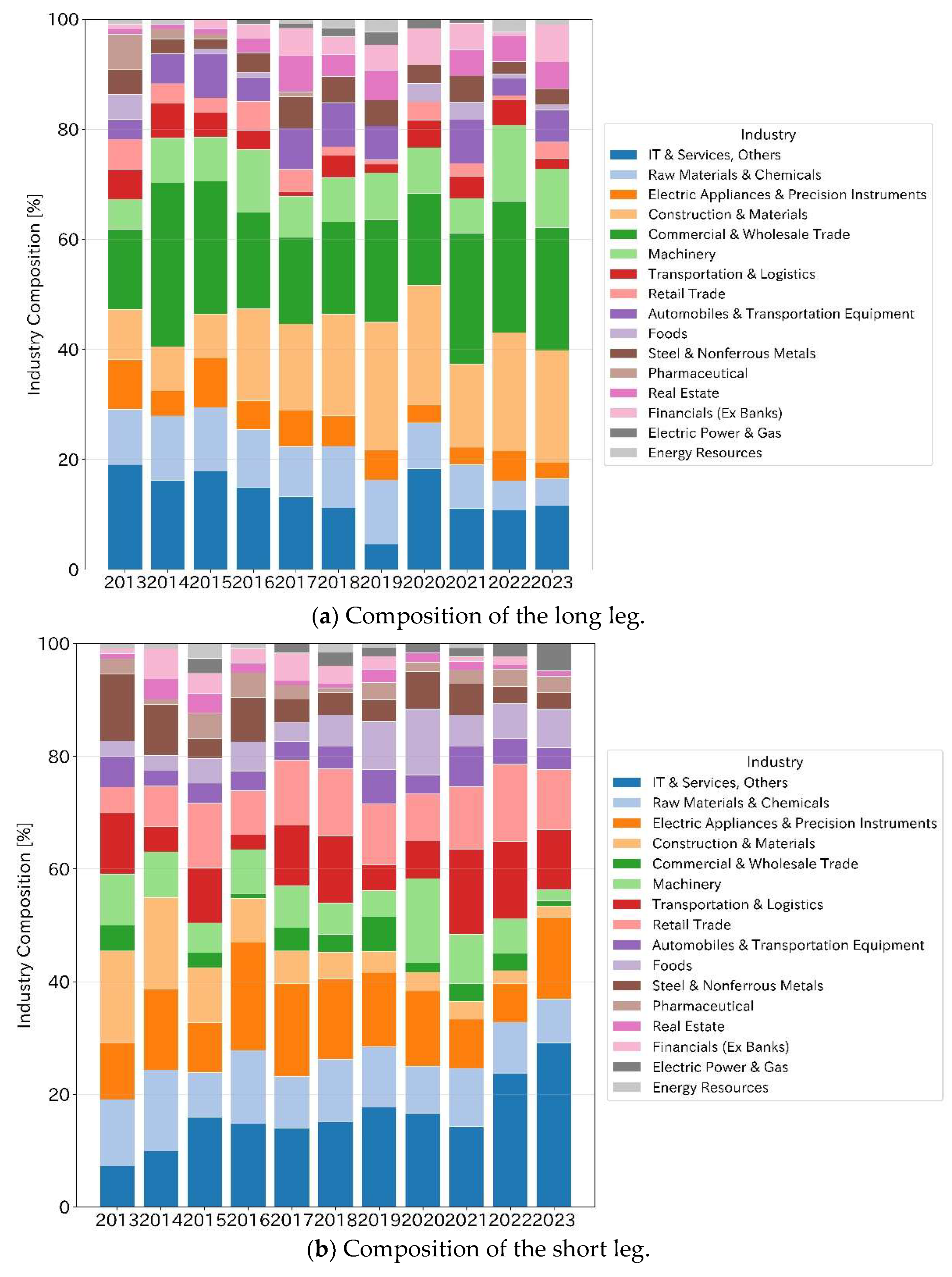
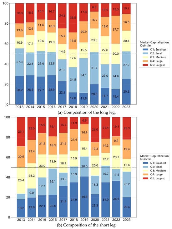
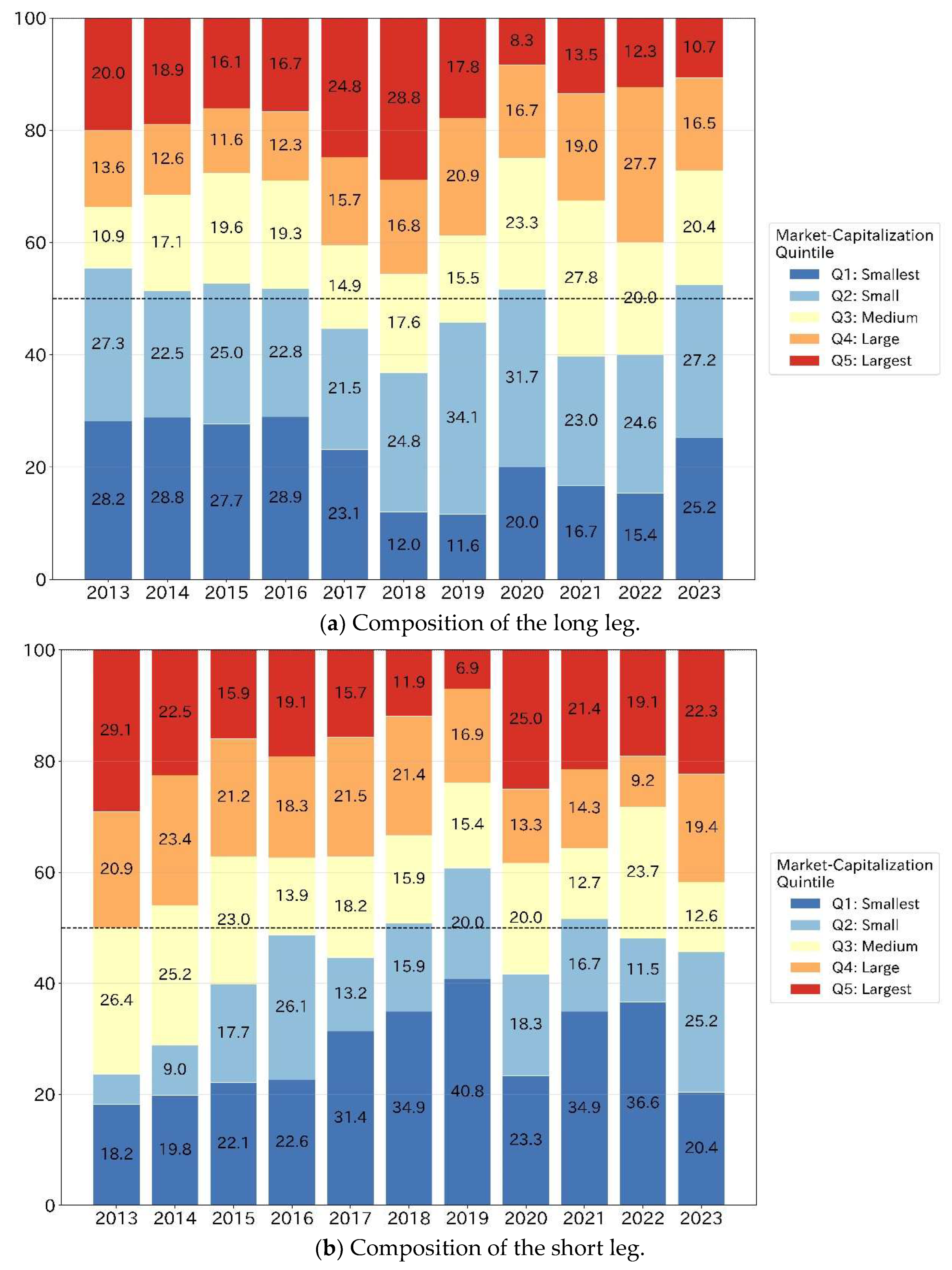

Disclaimer/Publisher’s Note: The statements, opinions and data contained in all publications are solely those of the individual author(s) and contributor(s) and not of MDPI and/or the editor(s). MDPI and/or the editor(s) disclaim responsibility for any injury to people or property resulting from any ideas, methods, instructions or products referred to in the content. |
© 2026 by the authors. Licensee MDPI, Basel, Switzerland. This article is an open access article distributed under the terms and conditions of the Creative Commons Attribution (CC BY) license.