


Abstract
After a benchmark decline, is the Robinhood holder-count addition rate higher in a +3× fund than in its unlevered counterpart, relative to an equal gain? Platforms list these funds side by side; the answer bears on sales-practice regulation. A fixed-effects panel regression relates that rate to lagged benchmark gains and declines by leverage target, using the 2018–2020 Robintrack archive, session-aligned and screened for instrument breaks and outages. The prospectively specified test fails to establish the predicted asymmetry. On eight exact-benchmark ladders, the 2% contrast is 0.59 additions per 1000 prior holders; its interval admits meaningful asymmetry of either sign, so this is not evidence of symmetry. A prespecified secondary contrast on 16 segments is 5.5 per 1000 but does not test the hypothesis; exploratory checks trace it to four added +3× segments, and it falls to 2.5 without changes spanning the prior close. Because a +3× fund’s own return is about three times its benchmark’s, the design cannot separate leverage preference from a response to that return. The study documents how product selection and measurement shape these comparisons. For regulators, a class-level holder-count asymmetry alone is not evidence of retail leverage-seeking.
Keywords:
retail investors; leveraged exchange-traded funds; holder counts; investor attention; pre-analysis plan; estimand sensitivity; data integrity JEL Classification:
G11; G23; G41
1. Introduction
Retail brokerage platforms offer both conventional and leveraged exchange-traded funds (ETFs) that track the same benchmark. An investor seeking broad equity or Treasury exposure may choose an unlevered fund, a +2× fund, or a +3× fund targeting a multiple of the benchmark’s daily return. Because these products share a benchmark and differ in their stated leverage target, their holder-count additions after benchmark moves show how measured participation varies across leverage targets. The question also bears on regulation: the Securities and Exchange Commission’s Rule 18f-4, adopted in October 2020, left the proposed companion sales-practice rules unadopted (U.S. Securities and Exchange Commission, 2020), and FINRA’s Regulatory Notice 22-08 subsequently solicited comment on complex products offered through self-directed platforms (Financial Industry Regulatory Authority, 2022). Both developments postdate the sample.
This study deliberately asks a narrow, reduced-form question: Within exact-benchmark long ETF families, is the gap between the +3× and +1× holder-count addition rates wider after a 2% benchmark-proxy decline than after an equal 2% benchmark-proxy gain? The evidence is platform-wide aggregate holder counts, the number of Robinhood accounts holding each fund, retrieved roughly hourly and assembled here into trading-session windows. Holder counts reveal how many accounts hold a fund, but not position sizes, purchase prices, or account identities. Therefore, a benchmark-proxy decline denotes a down-market state rather than an observed loss for any investor, and that distinction holds throughout the paper.
One limit governs everything below. Within a family-session, the benchmark move is common to the three funds, but a +3× fund’s own return is, up to tracking error, about three times its benchmark’s, so a response to the leverage target and a response to the fund’s own larger move are close to the same regressor in this design. The funds also differ in price, fees, age, liquidity, issuer, marketing, and prominence on the platform, and with one designated fund per leverage target in each family, this design does not credibly separate these attributes from the leverage target without further assumptions. The contrasts reported here are therefore reduced-form differences across leverage targets. They show whether holder-count additions differ across leverage targets after declines and gains. They cannot show that leverage is the reason.
Approach. This study proceeds in four steps, summarized in Figure 1. First, I rebuild the public Robintrack archive of approximately hourly Robinhood holder counts (May 2018 through August 2020) on a New York trading-session clock and screen it for instrument breaks at corporate actions and for collection and platform outages (Eaton et al., 2022). Second, I group funds into exact-benchmark families, verified against issuer filings, each with designated +1×, +2×, and +3× funds. Third, a three-way fixed-effects panel regression relates each fund’s holder-count addition rate to the previous session’s benchmark-proxy gain or decline, separately by leverage target. The tested quantity is one contrast: the +3×-versus-+1× response to a 2% decline minus the response to a 2% gain. Fourth, inference treats the families as fixed and calibrates the critical value by resampling blocks of sessions (Section 4.3). The sample, model, contrast, inference, and seven-test secondary family were prospectively specified in an analysis plan time-stamped on the Open Science Framework (OSF) on 31 August 2026, before any outcome-return estimation1. Analyses not in the plan are labeled exploratory, and outputs specified in the plan but computed later are marked as such.
Figure 1.
Research Design. Note. (A) Data sources, session panel, samples, and the primary model and test; the dashed line marks what the analysis plan fixed before any outcome-return estimation (time-stamped on OSF on 31 August 2026; Section 4.4), and the strip shows whether each tier of analysis is the primary test, a secondary test or mandatory output, or exploratory. (B) When the benchmark-proxy returns are measured relative to the window in which holder-count changes are counted; the lagged return is the one used in the primary test, and the contemporaneous and lead returns enter the timing checks. The panel also separates changes that span the prior session’s close from those recorded within the session. Poll ticks are schematic and follow the stamp audit shown in Supplementary Table S12.
The primary test did not establish the predicted asymmetry. The contrast is 0.59 additions per 1000 prior holders, and the interval reported under the prespecified calibration ranges from −2.62 to 3.80 per 1000 prior holders. This result is a failure to establish the hypothesized asymmetry rather than evidence that holder-count additions respond equally to declines and gains: no equivalence margin was prespecified, the interval contains differences of either sign, and its upper limit is approximately 30% of the mean daily +3× addition rate. This is the primary finding.
Other estimands provide different answers, and none of them replaces the primary one. A prespecified secondary test on a wider menu of 16 exact-benchmark segments gives 5.5 additions per 1000 and is the only rejection in its seven-test Holm family. It does not test the primary hypothesis (H-A; Section 2.4). Exploratory checks trace it to the four added +3× segments, and it falls to 2.5 once holder-count changes that span the prior close are excluded (Section 5.2). Adding the fund’s own return limbs moves it from 5.5 to 0.1 per 1000 and raises its standard error more than fourfold (Section 5.4). Among the three unlevered S&P 500 funds, SPY’s holder-count additions tilt toward declines relative to VOO’s by 1.5 per 1000; thus, product-specific differences arise without any leverage, and that comparison is not a control for prominence. The holder-count removal-rate contrast in the primary sample is negative but not a rejection under the prespecified multiple-testing adjustment; it is a suggestive pattern only.
This study makes three contributions, each reduced-form. First, it reports a prespecified test within exact-benchmark menus. Egan et al. (2022) use demand across same-benchmark funds with different payoff transformations to recover beliefs and risk tolerance; this study adds a daily, sign-conditional comparison of holder counts across leverage targets within the same benchmark and session, with the hypothesis, estimator, and inference fixed in advance and the interval reported in economic units. Second, it provides a reduced-form estimand map: a set of explicitly defined participation comparisons across product sets, weighting schemes, outcome scales, and measurement rules, against which class-level claims can be read. Murray and Sammon (2026) document contrarian dollar flows into long leveraged ETFs, Gempesaw et al. (2024) document return chasing in retail ETF order flow, and Bejar-Garcia (2026) reports sign-asymmetric holder growth by ETF class on this archive. On one audited dataset, the size and statistical detectability of the decline-versus-gain difference change across the comparisons in that map. Third, it documents an integrity audit of the Robintrack ETF series (instrument breaks at reverse splits, outages, and holder-count changes that span the session boundary), building on the stock-side uses of the archive (Ardia et al., 2025; Barber et al., 2022; Welch, 2022), and supplies an effective-dated ledger for later users.
The estimates do not identify a mechanism, and this study does not adjudicate among loss-conditioned risk taking, asymmetric loser attention, rebound beliefs, affordability, prominence, curation, or a changing entrant mix. Section 2 develops the prespecified prediction. Section 3 and Section 4 present the data, design, and inference. Section 5 reports the results. Section 6 discusses the interpretation and limitations. Section 7 concludes.
2. Literature Review and Hypothesis Development
This question sits at the intersection of limited attention, retail use of embedded leverage, and reference-dependent risk taking. Studies in these areas yield competing predictions for the relative response to equal-sized gains and declines, and several mechanisms predict the same sign, which is why the prespecified prediction is stated in reduced form.
2.1. Retail Attention, Salience, and Robinhood Holder Counts
Limited attention helps explain why individual investors disproportionately buy securities that have recently become salient. Barber and Odean (2008) show that attention affects buying more strongly than selling because investors face a much larger search set when choosing what to buy; thus, extreme returns, media coverage, and unusual volume can act as choice-set filters. The Robintrack archive made one extensive-margin measure of the process visible: the number of Robinhood accounts holding each security. Barber et al. (2022) document attention-induced herding around extreme returns; Welch (2022) characterizes the composition of the Robinhood crowd during the COVID-19 period; and Garcia (2026) studies stock-level attention dynamics in the same archive.
Barber et al. (2022) describe the Robinhood Top Movers list for the period as the 20 stocks with the largest absolute percentage price changes from the prior close, sorted without regard to sign. Whether leveraged ETFs were eligible for that list is undocumented; therefore, screen-based attention is a possible explanation rather than a measured channel.
The sign of the response is central. A simple magnitude-salience account predicts stronger participation after large absolute moves regardless of the sign. In contrast, Ardia et al. (2025) find, using high-frequency Robinhood data, that buying after extreme negative returns is stronger than after extreme positive returns. Therefore, sign symmetry cannot be assumed as a background condition, and a loss-versus-gain difference cannot, by itself, be interpreted as a change in risk preference.
2.2. Leveraged ETFs, Retail Product Choice, and the Exact-Benchmark Menu
Leveraged exchange-traded products target multiples of a benchmark’s daily return using derivatives, borrowing, and daily rebalancing, so that compounding can make multi-day performance diverge materially from the stated multiple (Cheng & Madhavan, 2009; Pessina & Whaley, 2021). Embedded leverage differs from margin borrowing in a behaviorally useful way: investors select a security whose payoff transformation is explicit in the product design. Account and order evidence indicates that these products attract distinct types of traders. D’Hondt et al. (2021) associate leveraged-product trading with poor performance and speculative characteristics; Davydov and Peltomäki (2023) show that adverse performance is attenuated among investors who closely monitor their portfolios; Arnold et al. (2022) show that attention triggers can increase risk taking; and Gempesaw et al. (2024) document substantial retail use of leveraged and inverse ETFs, together with return chasing in marketable order flows.
Murray and Sammon (2026) show, across the 2006–2025 leveraged ETF universe, that fund-level net flows into long leveraged ETFs are contrarian relative to the fund’s own recent returns, whereas flows into large unlevered ETFs chase returns. This evidence measures dollar creations and redemptions rather than holder counts, compares products across benchmarks rather than within exact benchmarks and sessions, and estimates linear return slopes rather than an equal-magnitude decline-versus-gain contrast; therefore, a contrarian slope pooled across products and a within-ladder difference across leverage targets are distinct objects.
ETF competition also makes product prominence a substantive alternative explanation of any gradient across leverage targets. Ben-David et al. (2023) show that funds compete for attention, and an exact benchmark match holds the underlying exposure constant while allowing visibility, age, brand, fees, and platform placement to vary. Section 5.4 compares three unlevered S&P 500 funds. This comparison shows that a decline-versus-gain difference can arise between products with the same leverage target; it does not measure prominence and is not a control for it.
The closest design precedent is Egan et al. (2022), who used retail demand across index funds that share a benchmark but transform its payoff differently, including differently levered S&P 500 funds, to recover expectations and risk tolerance. Their work shows that leverage choice alone cannot identify risk appetite: beliefs and preferences jointly enter demand. This study complements that work with daily holder counts, multiple exact-benchmark families, and an equal-magnitude decline-versus-gain contrast with fixed effects for the common family-session state. Bejar-Garcia (2026) is the nearest study on the same archive: it classifies ETFs into broad classes, relates holder-count growth to own-fund returns without day fixed effects, and reports both-sign growth with a stronger gain-side response among long-leveraged funds. Because a +3× fund targets a larger absolute daily return than a +1× fund for the same benchmark move, and because class models combine benchmarks, this study uses benchmark-proxy return limbs and exact-family comparisons.
2.3. Reference Dependence and Competing Explanations
Prospect theory holds that outcomes are evaluated relative to a reference point, with differing sensitivity to gains and losses (Kahneman & Tversky, 1979). Thaler and Johnson (1990) show that prior outcomes can affect subsequent risky choices through both a break-even motive after losses and a house-money effect after gains, mechanisms that point in different directions in the present contrast. Field evidence narrows what a market-level state can reveal. Imas (2016) shows that risk taking after losses depends on whether the loss was realized; Kumar (2009) documents persistent heterogeneity in lottery-stock preferences; and Suhonen and Saastamoinen (2018) show that break-even seeking need not select the riskiest available wager.
Reference dependence also affects the exit margin. Odean (1998) documents that individual investors realize gains more readily than losses, and Ben-David and Hirshleifer (2012) show that selling probabilities are V-shaped in returns since purchase. If a benchmark decline places more holders of the higher-leverage fund below their reference points, reference-dependent selling could lower that fund’s holder-count removal rate, which motivates the prespecified one-sided sign of the holder-count removal-rate contrast. The Robintrack data reveal none of the account-level states that condition these mechanisms (whether a holder gained or lost, whether a loss was realized, or whether an addition came from an incumbent or new entrant). Therefore, a lower holder-count removal rate in a down-market state is not evidence of a disposition effect or an attempt to break even.
Despite these limitations, several mechanisms are mapped onto the primary contrast. Magnitude-only salience predicts little difference between equally sized gains and declines. Loss-conditioned risk taking or rebound beliefs predict a positive loss-minus-gain difference, and asymmetric attention to losers predicts the same sign without changing risk tolerance, because the +3× fund’s own decline is mechanically larger and correspondingly more salient. Strong house-money or return-chasing responses predict a negative difference, and prominence or curation can amplify any of these if visibility varies with the leverage targets. Family-by-session effects hold common benchmark news constant but leave own-return salience, nominal price, age, issuer, familiarity, and placement free to vary. The directional hypothesis is therefore a prespecified reduced-form implication: rejecting in the predicted direction would be consistent with loss-conditioned participation without identifying it, and failing to reject would not demonstrate that any mechanism is absent.
2.4. Prespecified Prediction and Reporting Commitments
The directional prediction was fixed before estimation. Let Δ3(x) denote the modeled +3×-versus-+1× addition-rate response to a benchmark-proxy decline of magnitude x minus the response to a gain of the same magnitude (Section 4.2). The prespecified evaluation point is x = 2%.
H-A (prespecified confirmatory prediction). Within exact-benchmark long ETF families, the +3×-versus-+1× holder-addition-rate response to a 2% benchmark-proxy decline is more positive than the corresponding response to a 2% benchmark-proxy gain; equivalently, Δ3(2%) > 0.
H-A is a statement about a difference in holder-count addition rates across leverage targets. It is silent on why such a difference would arise, and without further assumptions, this design does not attribute one to leverage as opposed to the +3× fund’s larger own return or to any other attribute of the funds.
The primary test was two-sided at the 5% level, with support requiring both rejection and a positive estimate. H-A is the sole primary confirmatory hypothesis, and a positive contrast is not mechanism-specific. Two prespecified reporting rules accompany it. H-L permits a positive loss-side participation interpretation only if H-A is supported and the separately reported loss-side component is positive and rejects its own calibrated test. H-M requires that the +2× estimates be reported alongside the +3× estimates to describe the dose profile with no separate decision rule. The labels H-A, H-L, and H-M are the analysis plan’s own and are retained to make the reporting commitments traceable to the plan.
3. Data, Sample Construction, and Measurement
3.1. The Robintrack Archive
Robintrack was an independent service that polled Robinhood’s public interface roughly hourly from 2 May 2018 to 13 August 2020 and recorded the number of Robinhood accounts holding each listed security. The archive is public, contains no account identifiers, position sizes, or transactions, and aggregates behavior at the platform-by-security level.
Holder counts measure participation breadth. A single fractional share and a concentrated position register identically, and the archive reveals neither dollar exposure nor the identities of the accounts entering or exiting a position. Therefore, every result in this paper is a statement about participation counts, with capital flows unobserved.
3.2. Exact-Benchmark Families
An observation is a fund-session. Funds are grouped into exact-benchmark families, sets of long ETFs with identical stated daily benchmarks and differing leverage targets, and a cell is the designated fund at a given leverage target within a family. A family with designated +1×, +2×, and +3× funds is a complete ladder; a pair joins an unlevered anchor with a single +2× or +3× fund on the same benchmark; and a segment is either a ladder or a pair. The primary sample comprises eight complete ladders: six equity-index families and two Treasury families. Table 1 reports the roster, sample coverage, and return support by family.
Table 1.
Exact-benchmark families: roster, sample coverage, and 2% return support.
Family membership was verified rather than assumed. Each fund’s benchmark identity and leverage target were confirmed against prospectuses and issuer disclosures found via the SEC EDGAR full-text search system, with the verification source recorded fund by fund, and leverage targets were effective-dated (Supplementary Note S2). When a family contained more than one fund at the same leverage target, a single fund was designated in advance, and duplicates (for example, IVV and SPY at +1× on the S&P 500) were reserved for diagnostics.
A prespecified extension widens the menu. The all-valid-segments sample, hereafter the 16-segment sample (secondary test S6), adds a ninth complete ladder on the Russell 2000 and seven exact-benchmark pairs, each pairing an unlevered anchor with a single +2× or +3× fund (Table 1, Panel B). The roster was fixed in machine-readable form before estimation, including its one-window restriction: the Technology Select Sector +3× fund (TECL) enters through 21 April 2020, ahead of its issuer’s reverse-split batch.
3.3. Session Alignment and Outcome Measurement
The raw archive consists of irregularly spaced holder-count stamps in Coordinated Universal Time (UTC), whereas the behavioral question concerns responses to daily benchmark returns. All observations were therefore reconstructed using a New York trading-session clock. For each fund and NYSE session t, the end-of-session holder count Ht is the last stamp at or before the scheduled exchange close: 4:00 p.m. Eastern on regular sessions and 1:00 p.m. on the six early-close sessions in the sample. The session’s measurement window is the interval between the prior session’s scheduled close and the current one (Figure 1B). The rebuilt panel spans 576 NYSE sessions, explicitly handling holidays and early closes.
The outcome is a holder-count addition rate. Within each session’s measurement window, the positive inter-poll changes in a fund’s holder count were summed to form additions At, and the absolute values of the negative changes were summed to form removals Rt. Each change was assigned to the window containing its later observation, and each sum was scaled by the prior session’s closing holder base, yielding a holder-count addition rate At/Ht−1 and a holder-count removal rate Rt/Ht−1. By construction, At − Rt equals the net change in holders; thus, the two components are lower bounds on gross entry and exit events: offsetting changes between consecutive polls are unobserved. The addition rate does not identify unique new investors, can include repeated entries by the same account, and does not detect additional purchases by continuing holders. Changes that span the window’s opening boundary at the prior scheduled close are assigned to the current session; Table A1 reports their share of measured additions alongside stamp counts.
Robintrack recorded holder counts roughly hourly. Earlier users of the archive reported that stamps arrive at approximately 45 min past the hour and that the underlying Robinhood figure lags the stamp by approximately 30 to 45 min (Ardia et al., 2025; Barber et al., 2022). For the 22,466 fund-sessions of the 16-segment estimation sample, the last stamp at or before the prior scheduled close falls a median of 14.5 min before it (5th to 95th percentile, 8.8 to 17.7), and the next stamp follows by a median of 45.6 min (Supplementary Table S12). In 4.1% of those fund-sessions, the spanning interval exceeds 75 min (median about six hours, mostly before the close), so the spanning change then covers part of the preceding session’s trading hours; these observations carry 11.4% of measured spanning additions. The delay for individual records in this sample was not observed and may have varied. Under delays of the reported size, the inter-poll interval that spans the prior scheduled close can overlap the end of the preceding session; therefore, a change recorded in that interval may predate the close, follow it, or both. The archive does not show when within an inter-poll interval a change occurred.
Benchmark returns are proxied at the family level. Because several stated benchmarks are total-return or otherwise not directly investable, the benchmark-proxy return for family f in session t is the adjusted-close return (Yahoo Finance, retrieved with the quantmod package) of the family’s designated +1× anchor. Murray and Sammon (2026) use the same tradable-proxy convention for index products. A benchmark-proxy decline is a down-market state defined in Section 1.
3.4. Archive Integrity: Instrument Breaks, Large Holder-Count Changes, and Outages
The Robintrack archive identified each series using a Robinhood instrument identifier rather than a ticker symbol, and corporate actions that create a new instrument break the series in ways that matter for any ETF application. I hand-collected an effective-dated ledger of reverse splits, leverage changes, and delistings from issuer press releases and EDGAR filings and reconciled it with the raw series. Table 2 summarizes the census, and Figure 2 shows the observed coverage spans.
Table 2.
Archive-integrity census: instrument breaks, large holder-count changes, and outages.
Figure 2.
Robintrack Coverage by Ticker: Observed Spans, Reverse Splits, and the March–April 2020 Crash Window. Note. The bars show the observed spans, markers show reverse splits, and shading marks the March–April 2020 crash window. Gaps longer than one week are drawn, so the seven-session universal collection outage of January 2020 appears as a gap in every series observed at the time, whereas the three-session outage of January 2019 does not.
Within the mapped estimation universe, every series affected by a reverse split is missing either its pre- or post-split history; none spans its own split. Of the 38 dated ledger entries reconciled in Table 2, 15 trigger a series restart, in which the archive retains only the post-split instrument, and 13 trigger a series end, in which it retains only the pre-split instrument. The remainder concerns JNUG’s earlier split, the archive-adjacent USO and UCO series, which continue through their splits with large in-series holder-count jumps (Supplementary Note S2), and seven funds outside every estimation sample.
The timing of these breaks matters. Fifteen of the 28 dated truncation events occurred in March and April 2020, at the height of the COVID-19 crash and recovery, and the direction of the loss varied within a product complex: DUST, NUGT, and JNUG began on 23 April 2020, whereas JDST ended the same day. A class-level panel built naively from these files does not fail; it silently drops part of the crash-period history of some widely held leveraged products without an explicit sample decision (Section 5.5).
Collection and platform outages receive prespecified treatment. Ten NYSE sessions contained no stamps for any ticker (three in late January 2019 and seven in early January 2020). Observations adjacent to any collection gap were flagged and excluded: on such days, 11% of measured additions sat on the gap boundary, compared with 0.2% on normal consecutive days, indicating that a resume-day window accumulates several days of changes. Requiring consecutive sessions therefore keeps changes accumulated during collection gaps out of a daily outcome.
Robinhood’s platform outages on 2 March and 9 March 2020 are a distinct problem because they suppress trading itself rather than its measurement (Eaton et al., 2022). Both outage sessions and subsequent sessions were therefore excluded by prespecification, so that no day-by-day judgment about the direction of distortion enters the estimates. Finally, a gross-integrity screen, calibrated on a deliberately retained bad-series exemplar, was applied to every candidate series (Supplementary Note S2).
3.5. Estimation Samples and Descriptive Rates
The primary sample applies the prespecified inclusion rules. A fund-session enters only if the observation immediately follows the preceding session (no gap), is not adjacent to a collection outage, is not the fund’s first observation, has a prior holder base of at least five accounts, and has both lagged and contemporaneous benchmark-proxy returns defined. Family-sessions enter only when all three cells pass, and the four platform-outage-related sessions in March 2020 are removed. The sample is balanced across leverage cells within each retained family-session and nearly balanced across families, with 13,242 cell-session observations across 552 sessions. Supplementary Table S1 shows the full attrition path from 13,559 candidate consecutive-observation pairs through each rule, along with the reconciliation of the 576 rebuilt sessions to the 552 analysis sessions.
The China family is two sessions short of the common calendar because of a one-session XPP collection gap (Table 1, note). The 16-segment sample applies the same rules segment by segment, requiring each segment’s full roster to pass within a family-session, and contains 22,466 observations across 16 segments. Neither sample winsorizes or trims any outcome or return observations.
Table A1 reports additions, removals, boundary shares, holder bases, and stamp counts by family and leverage target. Three descriptive facts frame these results. The mean daily holder-count addition rate rises with the leverage target, from 5.3 per 1000 prior holders in the +1× cells to 11.1 in the +2× and 12.7 in the +3× cells. Holder bases are very small in several leveraged cells: the +2× Treasury and Emerging Markets funds average fewer than 25 holders, which is why the H ≥ 5 threshold was retained rather than being raised. The equity families have 22 to 45 sessions per sign with lagged benchmark-proxy returns at or beyond 2% in magnitude, whereas the Treasuries are sparser, with seven decline and 11 gain sessions for the 20-year family and only one and two for the 7–10-year family (Table 1). The model uses the full return distribution; therefore, these counts indicate how far the evaluation point rests on the functional form.
4. Research Design and Inference
4.1. Model Specification
The design compares holder-count addition responses across leverage targets within a family-session, holding the common benchmark state fixed and estimating only the relative response of the +2× and +3× funds. The model is a three-way fixed-effects panel regression on fund-sessions. Fund (cell) effects absorb time-invariant product differences in the level of the holder-count addition rate. Family-by-session effects absorb everything common to the funds on a benchmark in a session, which is why no un-interacted return term appears in Equation (1). Leveraged-status-by-session effects absorb shocks shared by leveraged funds across families. The coefficients of interest are therefore within-fund responses to the prior session’s benchmark-proxy return, compared across leverage targets within the same family and session. The fixed effects are removed by iterated weighted demeaning, the alternating-projections algorithm used by standard high-dimensional fixed-effects estimators. The estimator is weighted least squares only in the sense that it applies the prespecified equal-family weights; because the panel is almost balanced, those weights are nearly uniform, and the unweighted estimate is the same to the reported precision (Supplementary Table S4). The leverage target enters through indicators rather than a continuous term, leaving the +2× response unrestricted. The primary specification is as follows:
where i indexes funds, c indexes cells, f is the family of cell c, and t indexes NYSE sessions. Each cell holds one designated fund; therefore, index i is redundant and retained to match the analysis plan’s notation. The outcome is the holder-count addition rate At/Ht−1, in additions per prior holder; the text and tables report it per 1000 prior holders. The benchmark-proxy return rf,t is the close-to-close adjusted return of the family’s +1× anchor in decimal units, so that a 2% decline is r = −0.02. Lossf,t = max(−rf,t, 0) and Gainf,t = max(rf,t, 0) are its negative and positive return limbs, entered with quadratic terms to allow curvature; “Loss” is the plan’s variable name and denotes a benchmark decline rather than an investor’s loss. Both limbs are zero at r = 0; therefore, each modeled response is measured relative to a zero-return session. Dk(c) equals one when cell c holds the +k× fund. The +1× anchor is the omitted category, so every β, γ, δ, and λ is a difference from the +1× fund’s response in the same family-session, which is itself absorbed by μf,t. The β and γ coefficients are attached to the lagged limbs, and the δ and λ coefficients are attached to the contemporaneous limbs. The fixed effects are αc (cell), μf,t (family-by-session), and νL(c),t (leveraged-status-by-session, where L(c) equals one for the +2× and +3× cells and zero for the anchor); εi,c,t is the error term. Observations are weighted inversely to the family’s observation count and normalized to a mean of one. Δ2(x) is defined from the +2× coefficients in the same manner as Δ3(x) in Section 4.2.
Contemporaneous limbs are prespecified nuisance terms. Because the outcome window runs from the prior close to the current close, it includes the session-t return, and a response to that return would otherwise load onto the lagged limbs through serial dependence in returns; the family-by-session effects absorb only its family-common component.
What identifies the coefficients. Because the leveraged-status-by-session effects remove the session-wide average gap between leveraged and unlevered funds, a response shared by all leveraged funds when benchmarks move together is absorbed by design and is not part of the prespecified estimand. The coefficients are identified from the return variation that remains after the fixed effects and other included terms are partialled out. For the part of the response that the leveraged funds of a family share, that variation consists of differences across families within a session. The return support at the evaluation point is reported by family in Table 1; the 7–10-year Treasury family has one decline and two gains at 2%.
4.2. The Primary Contrast
The confirmatory quantity is an equal-magnitude model contrast. Define θL3(x) = βL3·x + γL3·x2 and θG3(x) = βG3·x + γG3·x2 as the modeled +3×-versus-+1× addition-rate responses for a benchmark-proxy decline and gain of magnitude x, and define Δ3(x) = θL3(x) − θG3(x). The evaluation point is x = 2%, chosen before estimation for adequate two-sided return support across the equity families. With returns in decimal units, Δ3(0.02) = 0.02(βL3 − βG3) + 0.0004(γL3 − γG3). Δ3(2%) compares modeled responses at equal magnitudes rather than matching individual gain and decline days. H-A predicts Δ3(2%) > 0, under the decision rule and reporting commitments of Section 2.4.
4.3. Calibrated Inference
Analytic inference clustered on families is poorly suited to this design: there are only eight family clusters, and session shocks common across families make them dependent. The families, a near-exhaustive selected set, are treated as fixed, and because the outcome is also serially dependent, the primary uncertainty calculation resamples blocks of sessions.
The prespecified decision rule. The tested quantity is the single linear contrast Δ3(2%). The statistic is its heteroscedasticity-robust (HC1) t-ratio, compared with c*, the 95th percentile of |t| for that same contrast across 2000 stratified moving-block resamples of the fixed-effect-projected outcome, using five-session blocks, strata defined by cell-availability patterns, and a resampling map that preserves cell identity. This is the rule fixed in the analysis plan, and the primary and secondary decisions are reported under it.
How the reported interval is built. The interval reported under the prespecified calibration is the estimate plus or minus c* times the HC1 standard error. The analysis plan called this construction a percentile-t interval; the computation is unchanged, and this paper uses the more exact name, a symmetric calibrated interval. This is an interval for that one contrast rather than a joint region for the return slopes. The Monte Carlo p value is (r + 1)/(S + 1), where r counts null draws at least as extreme as the observed statistic and S is the number of draws; a zero-exceedance result is reported as 1/2001, a reporting convention rather than evidence of exact test size. All resampling is deterministic under an archived seed.
What null the calibration imposes, and what that means for the interval. The prespecified resampling reassigns five-session blocks of the projected outcome to other sessions’ regressors. This sets every return slope to zero in the resampled data, not only the focal contrast, so the null it imposes is stronger than Δ3(2%) = 0. Reading the interval as a 95% interval for the contrast therefore rests on assumptions the procedure does not test: that the studentized statistic has approximately the same distribution when the other slopes are nonzero, and that the errors’ dependence and heteroscedasticity are not tied to the return path in a way that reassigning dates destroys.
Alternative inference for the same contrast. Three computations are set beside the prespecified result and kept distinct. Two impose only the focal restriction and keep residuals at their own dates. The archived block-wild residual diagnostic gives the same rounded critical value (2.10), with HC1 studentization and without reprojecting simulated outcomes through the fixed effects (Supplementary Table S3, which also reports the block-length and serial-dependence diagnostics). The contrast-specific wild bootstrap, added after the primary and secondary results were known and labeled exploratory, tests c′β = 0, where c is the vector of contrast weights and β the coefficient vector, while retaining the nuisance slopes: each draw applies a Rademacher sign to all restricted residuals within a five-session block and refits all fixed effects and slopes (9999 draws; ten- and twenty-session blocks leave both decisions unchanged). It yields a test, not an interval. The third computation imposes no null: a heteroscedasticity- and autocorrelation-consistent (HAC) covariance from the unrestricted model’s session scores (ten lags), with a normal-reference interval that is asymptotic rather than an inverted bootstrap confidence set (Table A2). For the primary contrast and S6, the decisions agree, and the intervals are close (Section 5.1 and Section 5.2). That agreement is a limited sensitivity check: it does not establish nominal coverage for any of these procedures and does not extend to the family-level or exploratory intervals computed with the prespecified algorithm.
Dependence-aware inference extends to exploratory analyses, and the multiplicity adjustment differs across sets of tests. The family-level, segment-level, lead-return, and group-difference quantities in Section 5 apply the calibrated algorithm to each quantity’s estimand, with its own critical value, and inherit the joint-null assumption. A simultaneous max-|t| critical value is reported for three sets only: the eight family contrasts, 16 segment contrasts (Table A3 and Table A4), and three S6 component contrasts (Supplementary Table S11). The remaining rows use standard errors clustered on five-session blocks, the bootstrap p values of Table A2 are unadjusted, and nothing is jointly adjusted across the exploratory battery; the Holm adjustment covers the decisions of the seven secondary tests, not their individual intervals. Supplementary Table S15 presents the inference key, and Table 3 lists the inference behind each principal quantity.
Table 3.
Estimand map: provenance, evidential role, and estimates of principal quantities.
The calibration changes the decision rule. On the frozen sample, the empirical 5% critical value was 2.07 under blinded calibration and 2.10 at estimation, and the measured size of a naive 1.96 rule was 6.1% under that simulation scheme. A prespecified family-sign cross-check treats families as clusters: a null-imposed wild cluster bootstrap-t over all 28 = 256 family-level sign assignments, studentized with a cluster-robust (CR1) variance (Cameron et al., 2008). The calibrated primary is the decision rule, and any disagreement between the two is reported.
4.4. Analysis Plan, Power, and Mandatory Robustness
The primary and secondary analyses were specified in an analysis plan time-stamped on OSF on 31 August 2026, before any outcome-return estimation. The plan and the files it governs were uploaded to OSF that day as a single archive, the plan package (https://osf.io/7kyd5 (accessed on 20 October 2026)). OSF lists the package with a single revision; a manifest inside the package gives the SHA-256 hash of every other file in it, so readers can check that the plan and code are the files time-stamped on 31 August (Supplementary Note S5 and Table S17). Throughout, “prespecified” and “prospectively specified” describe choices documented in the 31 August plan. Analyses added after the primary and secondary results were known are labeled exploratory and distinguished from exploratory analyses specified in the plan. The package includes the frozen sample definition, complete specification, deterministic calibration and estimation code, blinded power analysis, a seven-test secondary family with Holm adjustment (Holm, 1979), and explicit deviation rules requiring any result-informed change to be reported as exploratory. Before the plan was time-stamped, the estimator was tested only on resampled and day-permuted outcomes, and the day-permuted diagnostic did not reject. The plan carries the title “Benchmark Returns and the Leverage Gradient in Robinhood ETF Holder Additions.” The Data Availability Statement and Supplementary Note S5 give the history of the plan’s formal OSF registration.
The blinded power analysis characterizes the detection probabilities under simulated alternatives. Under both linear and quadratic injected alternatives, the minimum detectable Δ3(2%) at 80% power is approximately 3.8 additions per 1000 prior holders. A minimum detectable effect is not a bound; a non-rejection constrains the estimand only through its reported interval. Therefore, Section 5 presents the intervals in economic units.
Two estimator variants are mandatory robustness checks in the analysis plan’s terms: prespecified analyses that had to be reported, regardless of the results. A Poisson pseudo-maximum-likelihood (PPML) specification with the log prior holder base as offset (Santos Silva & Tenreyro, 2006) re-expresses the response on a proportional scale, and a linear-continuous-dose variant imposes the halfway +2× restriction that the indicator model relaxes. Both appear in Section 5.3. Because PPML targets a proportional conditional mean with model-implied weights, its estimate is read as a different estimand rather than as corroboration of the level-rate result. The plan’s other mandatory outputs (the components, the family-specific estimates, and the influence diagnostics) appear in Section 5.1, Appendix A, and the Supplementary Materials, and Supplementary Table S16 lists the interval reported for each prespecified quantity (the family-sign cross-check is reported as a test only).
4.5. Software and Use of Generative AI
All calibration and estimation code was written in Python (version 3.11.15) with NumPy 2.4.4 as its only external package, run with archived deterministic seeds; the session-panel build was verified on Python 3.10.12. Benchmark-proxy prices were Yahoo Finance adjusted closes retrieved in R (version 4.6.1) with the quantmod package (version 0.4.29), and figures were produced in Python with Matplotlib (version 3.10.9). The author used Claude (Anthropic; Claude Opus 5 model, accessed through the Claude desktop application) for data-engineering support, for drafting calibration and estimation code, for audits of the reported numbers, and for manuscript editing. The author specified each analysis before it was coded and reviewed the code, its outputs, and the findings of those audits, which checked every reported number against the archived machine-readable outputs. Supplementary Note S1 provides the verification steps.
5. Results
The primary test does not establish the predicted asymmetry: its contrast is 0.59 additions per 1000 prior holders, and the interval reported under the prespecified calibration admits differences of either sign (Section 5.1). A prespecified secondary test on a wider roster rejects its null; it does not test H-A and is sensitive to its roster and the outcome window (Section 5.2). Estimation followed the prespecified sequence: the primary contrast first, then the seven secondary tests, and then the mandatory and exploratory analyses. Supplementary Table S14 lists every correction and addition made after the primary and secondary results were known, including the corrected unlevered specification in Section 5.4.
Unless a row states otherwise, the estimates below are conditional differences in holder-count addition rates across leverage targets. The exceptions are labeled where they appear: the holder-count removal-rate and net log-change secondaries (S3 and S4), the proportional PPML contrast, the unlevered-fund comparison, and the class-level exercise. No mechanism is identified, and a non-rejection is not an equivalence result. Each reported quantity has two labels. Its provenance records how it was specified relative to the analysis plan: primary; secondary (seven tests in their own Holm family); mandatory robustness or mandatory output; exploratory, prespecified in the plan; or exploratory, added after the primary and secondary results were known. Its evidential role records what it can bear on: only the primary test supplies the decision on H-A, a rejection within the secondary family is a familywise rejection of that secondary null with no bearing on H-A, and the remaining rows are descriptive.
Two types of comparisons appear below and are read differently. Sensitivity checks keep the prespecified estimand and change how it is computed (the inference procedure, the block length, or the number of draws), and there, agreement with the prespecified result is informative. Every other row changes the evaluation point, the sample, the weights, the scale, the outcome window, the conditioning set, or another dimension named in Table 3, and thus targets a different quantity: agreement between such rows is not independent confirmation, a difference is not a contradiction, and two non-rejections are not evidence of equality.
Table 3 maps the principal estimands. Magnitudes are in additions per 1000 prior holders, unless stated, and two reference magnitudes recur: the equal-family mean daily +3× addition rate of 12.7 per 1000 and the median +3× cell-session rate of 6.5 per 1000.
5.1. The Primary Contrast and Its Components
Table 4 reports the primary results, and Figure 3A displays the pooled response curves underlying these results. The primary contrast is 0.59 additions per 1000 prior holders (p = 0.726). H-A is not supported. The interval reported under the prespecified calibration runs from −2.62 to 3.80 per 1000; its nominal coverage rests on the assumptions set out in Section 4.3, and a session-score HAC interval for the same contrast is −2.51 to 3.69 (Table A2). Both admit differences of either sign. The point estimate is under 5% of the mean daily +3× addition rate, whereas the interval’s upper limit is roughly 30% of that mean and 59% of the median +3× rate. Therefore, the estimate is near zero, yet imprecise enough to admit economically meaningful asymmetry of either sign. No equivalence margin was prespecified, and no equivalence claims were made. Counting only holder-count changes observed inside the session window, the same contrast is −0.70 per 1000 (p = 0.620; Table A2); thus, the positive sign of the primary point estimate itself depends on the window. For the primary contrast, the family-sign cross-check reached the same decision (p = 0.758).
Table 4.
Primary contrast and its components.
Figure 3.
Core Results. Note. (A) The pooled primary model’s +3×-versus-+1× addition-rate responses after benchmark-proxy declines (solid black) and gains (dashed gray) of magnitude x, shown as point estimates with the pooled return support (rug marks); the dotted line marks the prespecified 2% evaluation point, where the calibrated 95% intervals of the two components are drawn, set just left and right of the line so that they do not overlap (filled marker, declines; open marker, gains; Table 4). No pointwise band is drawn because none was calibrated for time dependence. (B) The primary and S6 estimates (filled squares), the exploratory interior-only S6 estimate (open square), family estimates (circles; decline/gain support counts at right), and added-segment estimates (triangles), each with its own calibrated interval; the intervals are individual and not simultaneous. The 7–10-year Treasury interval is clipped (arrows), and its marker sits at the estimate (−22.8). Under the simultaneous critical value across the eight family contrasts (4.21), no family estimate is individually significant.
The mandatory components show where the contrast comes from. The loss-side +3×-versus-+1× response at 2% is 2.66 per 1000 (SE = 1.51), and the gain-side response is 2.07 (SE = 1.23). Both components are positive, and neither rejects its own calibrated test (Table 4); therefore, the data do not establish a response on either side, and the H-L interpretation gate is not met. The point estimates are modeled +3×-minus-+1× differences relative to a zero-return session rather than total +3× addition rates or net holder growth.
Under the H-M reporting commitment, the +2× point estimates do not form a monotone dose profile: Δ2(2%) = −1.79 per 1000 (t = −1.09), with loss- and gain-side components of −1.45 and 0.34, respectively. The separate point estimates of this precision do not establish a non-monotonic response. Section 5.3 reports the mandatory continuous-dose restriction. At the exploratory 5% evaluation point, Δ3(5%) = −4.29 per 1000 (t = −1.17; interval −12.49 to 3.92), with the plan’s caveat that Treasury-family return support at that magnitude is effectively absent.
Common support at the evaluation point warrants direct examination. The Treasury families supply few sessions at or beyond 2% (Table 1), yet the plan gives them equal weight; thus, their contribution at the evaluation point rests on functional form. The 1% evaluation point (S1), where Treasury support is denser, yields 0.68 per 1000, and the family-volatility-scaled point (S2) yields 0.66. Dropping either Treasury family leaves the non-rejection unchanged: the estimate is 3.01 (t = 1.62) without the 20-year family and 0.04 without the 7–10-year family (Supplementary Table S6).
Excluding both Treasury families yields an exploratory contrast of 4.00 per 1000 (SE = 1.52; N = 9930; an HC1 t of 2.63 against a calibrated critical value of 2.18; p = 0.021). This contrast was added after the primary and secondary results were known and has no confirmatory weight. It shows that the pooled estimate and its non-rejection are sensitive to retaining, under the prespecified weighting, two Treasury ladders whose own estimates are negative and whose support at 2% is sparse (Table A3).
5.2. The Secondary Family
Table 5 reports all seven secondary tests, each with its own calibrated null and adjudicated jointly by Holm’s step-down procedure at a familywise 5% level. One rejects. S6 is a prespecified secondary test on an expanded roster, and its rejection is reported as the plan specifies. It does not test H-A, which is defined on the eight-ladder sample; its rejection cannot convert H-A into a supported hypothesis; and it identifies no mechanism. The estimate is 5.46 per 1000 (SE = 1.05), with an interval reported under its own calibration from 2.93 to 7.98 (session-score HAC interval, 2.96 to 7.96), a Monte Carlo p value below 0.001, and a Holm-adjusted p value of 0.003. In exploratory checks added after the primary and secondary results were known, it is 1.28 without the four added +3× segments, 2.26 without the biotechnology and semiconductor pairs (Table 6), and 2.46 when only holder-count changes observed inside the session window are counted (Table A2). Each deletion refits the model; therefore, these describe how the estimate moves and are not a decomposition. The rejection is a statement about this roster over this period, with uncertainty taken from time alone, and the added segments indicate where a difference appears.
Table 5.
Secondary family: seven tests, each with its own calibrated null, Holm-adjusted.
Table 6.
Sensitivity of the 16-segment contrast to sample, period, and roster variants (reference row, secondary test S6; other rows, exploratory).
With the sample, regressors, and weights held fixed, the 16-segment coefficient is the sum, before rounding, of a coefficient on changes observed inside the session window (2.46 per 1000) and a coefficient on the single inter-poll change that spans the prior close (2.99); therefore, the spanning changes account for 54.9% of the estimated coefficient. That percentage is an arithmetic share of a regression coefficient rather than a share of additions or of activity in any hour; spanning changes are 5.8% to 19.0% of measured additions across the 16-segment cells (Supplementary Table S12). For the interior-only contrast, the block SE is 0.95, the contrast-specific bootstrap p is 0.013 (Table A2), and the interval of the same construction as the prespecified one runs from 0.15 to 4.77 (Monte Carlo p = 0.036; Supplementary Table S11). Because the spanning interval can overlap the end of the preceding session (Section 3.3), part of the spanning component may be contemporaneous with the lagged return; the archive cannot apportion it. The decomposition is arithmetic rather than an estimate of measurement-error bias, and the interior-only outcome is an alternative measured outcome rather than a timing-corrected one: it keeps the prior holder-count denominator and remains subject to the archive’s polling schedule and reporting latency.
Differences across the segment groups can be tested directly. In exploratory comparisons within the 16-segment specification, the average contrast of the four added +3× segments exceeded the average of the original eight families by 9.9 per 1000 (an HC1 t of 5.81 against a calibrated critical value of 3.51; p = 0.006; contrast-specific bootstrap p < 0.001), and the sector-pairs-versus-broad-ladders contrast also rejected (5.4; p < 0.001). The two largest segment-level estimates belong to added +3× segments: biotechnology at 12.3 and semiconductors at 10.8. The other two added +3× segments, the Russell 2000 ladder and technology, are at 9.2 and 7.9 (Table A4). The broad-index ladders sit near their primary-sample values, and Treasuries remain negative. These comparisons do not explain why the groups differ.
Two further exploratory analyses are reported in Supplementary Table S11 under a reporting rule fixed before they were computed. The S6 loss-side component is 6.95 per 1000 (interval 4.48 to 9.41), and the gain-side component is 1.49 (−0.82 to 3.80), each defined as in Section 5.1; the H-L gate is conditional on H-A and does not apply to S6. A predefined grid crosses the roster and window sensitivities: counting interior changes only, the contrast is 0.49 per 1000 after removing the biotechnology and semiconductor pairs (block-clustered t interval −1.92 to 2.90; bootstrap p = 0.700), a roster that still holds the added Russell 2000 and technology +3× segments, and −0.15 after removing all four added +3× segments (−2.71 to 2.40; p = 0.915). The bootstrap p values come from separate tests and are not inverted into these intervals. Neither test rejects, and both intervals admit differences of either sign; therefore, these estimates establish neither a difference nor its absence.
The holder-count removal-rate contrast (S3) is −2.70 per 1000 (SE = 1.20). It rejects its own one-sided calibrated test (t = −2.25 against −1.88; p = 0.025) but not the Holm-adjusted test (p = 0.150); therefore, it is not a rejection within the secondary family. It is a suggestive holder-count pattern: measured removals from the +3× fund are relatively lower after benchmark declines than after equal gains. The archive records no purchase prices or returns since purchase; therefore, the pattern cannot be read as a disposition effect, and its difference from the addition-rate contrast has not been tested. The net log holder-count change (S4; Holm p = 0.355) is arithmetically linked to additions and removals and is not independent evidence.
Three further secondaries do not reject (Table 5): the 1% evaluation point (0.68), the family-volatility-scaled evaluation point (0.66), and the nine-ladder sample adding the Russell 2000 (1.09). They target different quantities; therefore, their non-rejections are not evidence that the primary contrast is zero. The common-hourly-grid reconstruction (S7) changes eight of the matched outcome values and admits six additional China cell-sessions because the hourly grid bridges the one-session XPP gap (N = 13,248). Its estimate is 0.60 against 0.59, which is a limited sensitivity check of polling cadence; the sum of positive inter-poll changes depends on polling frequency, so its measured outcome is not identical.
5.3. Estimand Dependence: Composition, Weighting, and Scale
This subsection isolates each dimension that can be isolated. Figure 3B shows the family and segment estimates with their individual calibrated intervals, and Table A3 and Table A4 list the full set with the simultaneous critical values.
Inference about family composition depends on the procedure. In a fully interacted specification on the primary sample, four families exceeded their own calibrated critical values: three positive (Nasdaq-100, Dow, and China 50) and one negative (the 20-year Treasury). The 7–10-year Treasury estimate of −22.8 per 1000 has a calibrated critical value of 4.02, reflecting its one decline and two gain sessions at 2% (Table 1). Supplementary Note S3 explains why the family critical values depart from the normal reference in both directions.
These own tests are descriptive, and for individual families, the familywise conclusion is the operative one: under the simultaneous critical value of 4.21 across the eight family contrasts, no family estimate is individually significant. The comparison of the equity and Treasury groups is a separate question, and neither result substitutes for the other. The equity-minus-Treasury average contrast is 19.43 per 1000. The calibrated test gives p = 0.113 (an HC1 t of 2.77 against a calibrated critical value of 3.55), the contrast-specific bootstrap gives p = 0.050 (Table A2), and the HAC interval is 8.47 to 30.39 (Supplementary Table S16). The evidence for this group difference therefore depends on the inference procedure. The comparison is exploratory and does not alter the primary decision. The pooled estimate (0.59) and the unweighted average of the family estimates (−0.50) are distinct objects because the pooled model restricts the limb coefficients to be common across families (Supplementary Note S3).
Weighting and scale are the operative dimensions of the map (Table 3; Supplementary Table S4). Replacing equal-family with equal-observation weights leaves the estimate at 0.59 (Section 4.1). Keeping the level-rate outcome and the model form, holder-base weighting targets a different weighted contrast, estimated at 4.75 per 1000 (block-cluster t = 3.36). Restricting the level model to the PPML-retained sample leaves the estimate nearly unchanged, at 0.56, so the 279 separation drops have little effect on the level-rate point estimate.
The mandatory PPML estimate is 0.378 log points (block-cluster SE = 0.106, t = 3.55; interval 0.167 to 0.589): the modeled +3×-versus-+1× conditional-mean addition ratio is approximately 46% larger after a 2% benchmark-proxy decline than after an equal gain (exp(0.378) = 1.46). The coefficient is not directly comparable to the level estimates because the units differ (Section 4.4). The equal-family level rate, holder-base-weighted level rate, and proportional conditional mean are three different targets, and their estimates differ.
The mandatory continuous-dose specification imposes a halfway +2× restriction on each return limb (Section 4.4). The implied +3×-versus-+1× contrast is 1.25 per 1000 in the primary sample (five-session-block SE = 1.76; contrast-specific p = 0.507; HAC interval −1.62 to 4.12), and an exploratory extension to S6 yields 6.05 (block SE = 1.24; p < 0.001). Direct tests of Δ3 − 2Δ2 = 0 do not reject in either sample (p = 0.300 and 0.179), so the evaluation-point restriction is not contradicted, although a single contrast does not test the stronger restriction on all return-limb coefficients (Table A2).
5.4. Own-Return Limbs, Unlevered Comparison, Timing Checks, and Sample Variants
Table 7 reports the correlated-channel specifications: descriptive reparameterizations that change the estimand and are near-collinear because a +3× fund’s own return is close to three times its benchmark’s. Within the fixed-effect space, own-return limbs explain 71% to 78% of the variation in the +3× benchmark-return limbs. With five-session-block-clustered standard errors, adding own-fund return limbs to the 16-segment specification moves the contrast from 5.47 per 1000 (t = 4.54) to 0.07 (t = 0.01), with a much larger standard error. The contrast changes little when abnormal volume is added (5.40) and rises when overnight-gap limbs are added (7.89). Because the leverage target ties each fund’s return closely to its benchmark, and the own-return specification is imprecise, the design does not credibly isolate leverage from the size of the fund’s own move without further assumptions.
Table 7.
Correlated-channel specifications, 16-segment sample (descriptive reparameterizations; exploratory).
Two further reparameterizations were added after the primary and secondary results were known, and they appear in Supplementary Table S9. Conditioning on the standardized lagged holder base gives 2.81 per 1000 in the primary sample (calibrated p = 0.134) and 6.51 in the 16-segment sample (p < 0.001), and adding the fund’s lagged tracking deviation gives 0.88 and 5.55, against 0.59 and 5.46 without it. Both rows change the estimand, and neither rules out familiarity, placement, or other forms of prominence. Tracking deviation is where a fund’s own return departs from the leverage multiple; its standard deviation is 0.33 to 0.35 percentage points, and the specifications that use it do not separate the leverage target from the fund’s own return.
Product-specific differences without leverage. Three unlevered S&P 500 funds (VOO, IVV, and SPY) share a benchmark and a leverage target, so a comparison among them asks whether a decline-versus-gain difference can arise with no leverage anywhere. The specification uses fund and session fixed effects, retains the lagged and contemporaneous return limbs, and has full rank. Across 1542 fund-sessions over 514 sessions, the SPY-minus-VOO difference at 2% is 1.48 per 1000 (five-session-block SE = 0.36; contrast-specific bootstrap p < 0.001), the IVV-minus-VOO difference is −0.09 (p = 0.801), and the SPY-minus-IVV difference is 1.57 (p = 0.003; Table A2). A product-specific difference of about 1.5 per 1000 therefore exists among funds that differ in volume, age, fee, and familiarity but not in leverage. The comparison is descriptive; it is not a control for prominence, and it does not measure the share of the 16-segment estimate attributable to non-leverage characteristics.
The prespecified session t + 1 lead-return check did not reject: 2.33 per 1000 (calibrated p = 0.115; interval −0.53 to 5.19; Supplementary Table S10). The session-t window closes before any part of the t + 1 return exists, which rules out the mechanical use of future prices but not common predictive states or unmeasured reporting latency. Among the six further lead variants in that table, one was a boundary result (2.85 per 1000; p = 0.048, with the lead limbs added to the prespecified model), and no other lead contrast was rejected. These checks qualify the timing interpretation but do not validate a causal design.
None of the prespecified exploratory sample variants produced a rejection of the primary contrast, and each block-clustered interval included zero (Supplementary Table S6): excluding the COVID-19 period, excluding the five largest S&P 500 decline sessions, retaining the March 2020 platform-outage sessions, raising the holder-base floor to 25 or 50, dropping any single family, and splitting on the prior-session VIX level or the fractional-shares introduction. Each changes the estimand, and none establishes a zero effect. The ten most influential observations, a mandatory output of the analysis plan, are listed in Supplementary Table S7.
Table 6 reports the selected period, decline-session, and roster variants for the 16-segment contrast, with calibrated inference for each subsample’s null. The point estimate is positive in both periods (5.99 per 1000 through 19 February 2020, and 4.21 in the COVID-19 period, where the test on 119 sessions does not reject), and a joint model does not detect a period difference (−1.78; contrast-specific p = 0.534, Table A2; HAC interval −7.51 to 3.96, Supplementary Table S16); neither non-rejection is an equivalence result.
A return-tail check excludes entire family-sessions whose absolute lagged benchmark return exceeds that family’s 99th percentile and recomputes the equal-family weights. The primary estimate becomes −0.07 per 1000 (contrast-specific p = 0.967; N = 13,098), whereas S6 is 5.24 (p < 0.001; N = 22,222); therefore, the 16-segment estimate is not confined to each family’s most extreme lagged returns (Table A2).
Each of the 16 leave-one-segment-out fits retained a positive estimate, between 3.59 and 7.46 per 1000, with a block-cluster t of at least 2.91 (Table 6). Joint deletions can materially change the estimate: without the biotechnology and semiconductor pairs, or without all four added +3× segments, no rejection remains (Section 5.2). These overlapping checks are not independent replications, and their own tests have no joint familywise adjustment.
5.5. A Class-Level Sensitivity Exercise
The analysis plan lists this item as a descriptive class-level replication of Bejar-Garcia (2026). It is reported here as a sensitivity exercise because the fund roster, filters, and controls differ from those of that study, and its results say nothing about whether that study’s estimates reproduce on its own sample. On the integrity-screened sample, a specification modeled on the prior study yields positive coefficients on both return limbs, and the difference between the loss and gain coefficients is not detected (0.011; two-way-clustered t = 0.49). Adding day fixed effects widens the difference to 0.043 (t = 0.90), and only under benchmark-proxy returns with day effects does the decline-versus-gain difference itself reject (0.110; t = 2.34). The difference is positive in every displayed specification, and its magnitude and statistical detectability change with the return measure and day effects; a rejection in one row and a non-rejection in another do not establish that the rows differ. Supplementary Table S8 reports the specifications and the class-level sample, which is not a superset of the confirmatory one.
6. Discussion
6.1. What the Estimates Can and Cannot Say
Claims about retail participation in leveraged funds depend on the products and participation measure used to construct them. The primary test does not establish the predicted asymmetry, and the size of the 16-segment contrast, which does not test H-A, depends on the added +3× segments and on changes that span the prior close. In the class-level exercise, the estimated decline-versus-gain difference likewise varies with the return measure and day effects (Section 5.5). Weighting and scale dependence are documented rather than tested because the holder-base-weighted and proportional-scale estimands are different functionals of the same observations. This paper states each estimand’s sample, weights, scale, and window, tests the differences that can be tested, and declines to average the answers into one number.
The unlevered comparison in Section 5.4 shows that a decline-versus-gain difference arises between S&P 500 funds with no leverage. These funds differ in volume, age, fee, and familiarity; therefore, the exercise identifies a product-specific difference, not a prominence effect or a quantitative bound on leverage’s contribution to the added-segment difference. Taken together, the exploratory exercises of Section 5.4 leave observationally equivalent readings of that difference: demand for embedded leverage conditional on down-market states, attention to the largest movers, rebound beliefs, product familiarity, and the dating of holder-count changes around the close. These readings cannot be distinguished with these data without further assumptions, and this paper claims none. Neither the dose profile nor the descriptive statistics of the added segments discriminate among these readings (Section 5.1 and Section 5.3; Table A5; Supplementary Note S4).
The same discipline applies to the contrarian fund-level flows that Murray and Sammon (2026) document for long leveraged ETFs. Net creations can rise after declines because entries rise, exits fall, or continuing holders add to positions, and a holder count cannot tell which. In these data, neither the addition-side components nor the holder-count removal-rate contrast is established at the prespecified error rate (Section 5.1 and Section 5.2), and linking this participation margin to dollar flows requires account or order data on position sizes.
6.2. Limitations
The primary and secondary analyses follow the plan and use dependence-aware inference. Several limitations bound the interpretation of the results. Leverage is not isolated. The leverage target ties the fund’s own return to approximately a multiple of the benchmark’s, and the own-return specification is too imprecise to tell a response to the leverage target from a response to the fund’s own move (Table 7). The collapse of the 16-segment contrast when own-return limbs are added is a property of the design rather than evidence that fund returns cause additions. The fund fixed effects absorb time-invariant differences in the level of additions, including those that come with fees, marketing, liquidity, and popularity. They do not absorb differences in how funds with those attributes respond to benchmark moves. Each family has one designated fund per leverage target; therefore, within a family, every such attribute moves one-for-one with the leverage target. This design therefore does not credibly isolate leverage from the fund’s own return or from these attributes without further assumptions. The estimates are differences across leverage targets, not effects of leverage.
Holder counts are breadth only. They cannot distinguish a fractional-share entry from a concentrated bet, separate entrants from incumbents, detect a continuing holder’s additional purchase, or reveal any investor’s reference point or realized outcome (Welch, 2022).
The outcome window matters. The addition and removal measures bound gross entry and exit events, offsetting changes between polls are unobserved, and the delay between observation and retrieval is not observed for the records in this sample. Boundary-spanning changes, whose timing within the spanning interval is unobserved, account for more than half of the estimated 16-segment coefficient; thus, the timing limitation is economically consequential rather than a data-description caveat.
Inference relies on a stated calibration. The prespecified calibration imposes a joint zero-return-slope null that is stronger than the focal contrast alone; its coverage for a single contrast is assumed rather than demonstrated. A focal-null bootstrap test and a separate session-score HAC interval are reported beside it; their agreement with it for the primary contrast and S6 is a limited sensitivity check and does not demonstrate coverage, and for the exploratory equity-minus-Treasury comparison, the procedures disagree (Section 5.3). No equivalence test supports the interpretation of the near-zero primary estimate as symmetry. The exploratory battery is large and grew after the primary and secondary results were known: only the seven secondary tests receive the prespecified Holm adjustment, and the exploratory tests are not jointly adjusted.
One platform and one period. The sample covers one platform over 27 months ending in August 2020, includes the COVID-19 crash, and reflects a user population that has since changed; therefore, generalization beyond the platform and period is conjecture.
The first two limitations correspond to concrete extensions. Independent variation in leverage and product visibility would help distinguish leverage preference from attention, and account-level holdings and transaction data would separate entrants from incumbents, distinguish new participation from changes in position size, and permit realized-loss conditioning in the spirit of Imas (2016).
7. Conclusions
This study contributes a prespecified, exact-benchmark comparison of holder-count additions across leverage targets, a reduced-form estimand map that places this comparison beside explicitly defined alternatives, and an audit of the instrument breaks, outages, and session-boundary conventions that later applications of the archive must address. It does not test why measured participation differs across the leverage targets. The question was deliberately narrow: within exact-benchmark long ETF families on Robinhood, whether the +3×-versus-+1× holder-count addition response is more positive after a 2% benchmark-proxy decline than after an equal gain. For the prespecified equal-family, level-rate estimand, the contrast is 0.59 additions per 1000 prior holders, with an interval reported under the prespecified calibration from −2.62 to 3.80 per 1000. The primary hypothesis was not supported, and the estimate did not establish symmetry. The interpretation gate for a loss-side participation claim is not met, and the negative holder-count removal-rate contrast is only a suggestive pattern.
The design limits the meaning of any of the estimates. Leveraged funds’ own returns are mechanically linked to their leverage targets, the funds differ in other attributes that move one-for-one with the leverage target within a family, and a decline-versus-gain difference also appears between two unlevered S&P 500 funds. Without further assumptions, the evidence therefore does not separate the demand for amplified exposure from attention, beliefs, or other product characteristics.
Other estimands provide other answers. The 16-segment secondary contrast (S6) is 5.5 per 1000 and is the one familywise rejection among the secondaries; it does not test the primary hypothesis. Exploratory comparisons trace it to the added +3× segments, and it is 2.5 per 1000 once changes that span the measurement window’s opening boundary are excluded, a reduction that does not measure bias because the timing of those changes is unobserved. Holder-base weighting and proportional-scale estimation target different quantities; their estimates are positive, and this paper does not average them.
For platform designers and regulators weighing the sales-practice questions that Rule 18f-4 left open and FINRA reopened, the caution is that a class-level asymmetry cannot be read as retail leverage-seeking without stating its products, sample, weighting, scale, and outcome window. For researchers who rely on found data of this kind, the results argue for prespecified estimands, dependence-aware inference, and integrity audits as standard practices. The cause of the added-segment difference remains open because the readings set out in Section 6.1 are observationally equivalent in these data. Account-level data, or variation in leverage that is independent of a fund’s return and visibility, are needed to distinguish them.
Supplementary Materials
The following supporting information can be downloaded at: https://www.mdpi.com/article/10.3390/ijfs14110290/s1. Note S1. Use of Generative AI and Verification Steps; Note S2. Archive-Adjacent Series and the Gross-Integrity Exemplar; Note S3. Mechanics: Fixed-Effect Removal, Block Resampling, Family Critical Values, and the Pooled Estimate; Note S4. Descriptives of the Added Segments; Note S5. Registration Record and Verification; Figure S1. Archive-Adjacent Series That Continue Through Their Splits; Table S1. Sample Attrition and Session Reconciliation; Table S2. Interior and Boundary Components of Additions and Removals, and Within-Family Addition Shares (Primary Sample); Table S3. Inference Diagnostics for the Prespecified Resampling Scheme; Table S4. Estimand Crosswalk by Sample, Weighting, and Scale, With HC1, Session-Clustered, and Block-Clustered Standard Errors; Table S5. Correlated-Channel Specifications, Primary Sample (Near-Zero Baseline; HC1 and Block-Clustered Standard Errors); Table S6. The Primary Contrast Under the Prespecified Exploratory Sample Variants (HC1 and Block-Clustered Standard Errors); Table S7. The Ten Most Influential Observations for the Primary Contrast (Mandatory Output); Table S8. Class-Level Sensitivity Exercise: Gain and Loss Limbs With Direct Difference Tests (Two-Way Clustered Standard Errors); Table S9. Holder-Base Conditioning and Tracking-Deviation Limbs, Primary and 16-Segment Samples (Exploratory; Added After the Primary and Secondary Results); Table S10. Lead-Return Variants (Exploratory; Calibrated Inference); Table S11. Interior-Only Intervals, S6 Components, and the Roster-by-Window Grid (Exploratory; Added After the Primary and Secondary Results); Table S12. Stamp Audit and Boundary-Spanning Shares of Measured Additions (Descriptive; Added After the Primary and Secondary Results); Table S13. Full Estimand Crosswalk, Keyed to the Identifiers of Table 3; Table S14. Ledger of Departures From the Analysis Plan and of Additions Made After the Primary and Secondary Results Were Known; Table S15. Inference Key: Statistic, Reference Distribution, Null Imposed, Interval Construction, and Multiplicity Family of Each Procedure; Table S16. Interval Inventory for the Prespecified Analyses, Keyed to the Analysis Plan, With the Archived Intervals for Table A2 and Table 6; Table S17. Registration Timeline and Its Sources.
Funding
This research received no external funding.
Institutional Review Board Statement
Not applicable. This study uses a public archive of platform-level aggregate holder counts that contains no account identifiers, position sizes, or transactions, and involves no interaction with human subjects.
Informed Consent Statement
Not applicable.
Data Availability Statement
The Robintrack holder-count archive is publicly available (robintrack.net). The SHA-256 hash of the exact archive object analyzed is recorded in the plan package, and a documented route to the identical object, verified by its SHA-256 hash on 20 October 2026, is included in the publication materials deposited at https://osf.io/knwjs (accessed on 20 October 2026). Benchmark-proxy prices were retrieved from Yahoo Finance in R 4.6.1 with quantmod 0.4.29, and the plan package documents the retrieval scripts, dates, adjustment conventions, and file hashes. The analyses were run in Python 3.11.15 with NumPy 2.4.4 (Section 4.5). The plan package also documents software versions, random seeds, the build entry point, the effective-dated family map, the corporate-action ledger, and the outage and session calendars; the machine-readable results behind every table and figure, and the scripts written after estimation, are deposited separately with those publication materials. The analysis plan, deterministic calibration and estimation code, blinded power analysis, and data manifests were time-stamped on the Open Science Framework on 31 August 2026, before any outcome-return estimation. An OSF technical archiving failure prevented completion of the registration initiated that day and delayed formal registration until 23 September 2026, after the primary and secondary results were known; the completed registration archives the package uploaded on 31 August (https://osf.io/7kyd5 (accessed on 20 October 2026)). Supplementary Note S5 gives the time stamps and the hash of the plan package, whose manifest lists the hash of every other file. No file in the plan package, and no file whose hash its manifest records, has changed since 31 August 2026.
Acknowledgments
During the preparation of this study, the author used Claude (Anthropic; Claude Opus 5 model, accessed through the Claude desktop application) for the purposes of data-engineering support, analysis-code drafting, audits of the reported numbers, and manuscript editing assistance, as described in Section 4.5. The author has reviewed and edited the output and takes full responsibility for the content of this publication.
Conflicts of Interest
The author declares no conflicts of interest.
Appendix A
This appendix holds the descriptive table behind the addition rates and the three sets of outputs on which the main text relies most: the contrast-specific inference, the family and segment estimates, and the segment descriptives. The remaining supporting tables, notes, and further exploratory analyses are in the Supplementary Materials. Table A1 and Table A5 are descriptive, and the estimates in Table A2, Table A3 and Table A4 are exploratory unless marked otherwise. Calibrated inference uses the prespecified stratified block-resampling algorithm applied to each quantity’s own estimand, and block-clustered standard errors cluster on five-session blocks.
Table A1.
Additions, removals, boundary shares, holder bases, and stamp counts by family and dose (primary sample).
Table A2.
Contrast-specific inference and measurement checks added after the primary and secondary results (exploratory).
Table A3.
Family estimates with calibrated inference: primary-sample families (simultaneous critical value 4.21).
Table A4.
Segment estimates with calibrated inference: 16-segment sample (simultaneous critical value 4.62).
Table A5.
Segment descriptives for the 16-segment sample: holder bases, benchmark-proxy volatility, own-return magnitude, and addition rates by segment and dose.
Note
| 1 | The Data Availability Statement and Supplementary Note S5 give the history of the plan’s formal OSF registration. |
References
- Ardia, D., Aymard, C., & Cenesizoglu, T. (2025). Examining high-frequency patterns in Robinhood users’ trading behavior. International Review of Financial Analysis, 105, 104369. [Google Scholar] [CrossRef] [Scilit]
- Arnold, M., Pelster, M., & Subrahmanyam, M. G. (2022). Attention triggers and investors’ risk-taking. Journal of Financial Economics, 143(2), 846–875. [Google Scholar] [CrossRef] [Scilit]
- Barber, B. M., Huang, X., Odean, T., & Schwarz, C. (2022). Attention-induced trading and returns: Evidence from Robinhood users. The Journal of Finance, 77(6), 3141–3190. [Google Scholar] [CrossRef] [Scilit]
- Barber, B. M., & Odean, T. (2008). All that glitters: The effect of attention and news on the buying behavior of individual and institutional investors. The Review of Financial Studies, 21(2), 785–818. [Google Scholar] [CrossRef] [Scilit]
- Bejar-Garcia, C. (2026). Retail asset class rotations: Evidence from ETFs (SSRN Working Paper No. 6424578). SSRN. [Google Scholar] [CrossRef] [Scilit]
- Ben-David, I., Franzoni, F., Kim, B., & Moussawi, R. (2023). Competition for attention in the ETF space. The Review of Financial Studies, 36(3), 987–1042. [Google Scholar] [CrossRef] [Scilit]
- Ben-David, I., & Hirshleifer, D. (2012). Are investors really reluctant to realize their losses? Trading responses to past returns and the disposition effect. The Review of Financial Studies, 25(8), 2485–2532. [Google Scholar] [CrossRef] [Scilit]
- Cameron, A. C., Gelbach, J. B., & Miller, D. L. (2008). Bootstrap-based improvements for inference with clustered errors. The Review of Economics and Statistics, 90(3), 414–427. [Google Scholar] [CrossRef] [Scilit]
- Cheng, M., & Madhavan, A. (2009). The dynamics of leveraged and inverse exchange-traded funds. Journal of Investment Management, 7(4), 43–62. [Google Scholar]
- Davydov, D., & Peltomäki, J. (2023). Investor attention and the use of leverage. Financial Review, 58(2), 287–313. [Google Scholar] [CrossRef] [Scilit]
- D’Hondt, C., McGowan, R., & Roger, P. (2021). Trading leveraged exchange-traded products is hazardous to your wealth. The Quarterly Review of Economics and Finance, 80, 287–302. [Google Scholar] [CrossRef] [Scilit]
- Eaton, G. W., Green, T. C., Roseman, B. S., & Wu, Y. (2022). Retail trader sophistication and stock market quality: Evidence from brokerage outages. Journal of Financial Economics, 146(2), 502–528. [Google Scholar] [CrossRef] [Scilit]
- Egan, M. L., MacKay, A., & Yang, H. (2022). Recovering investor expectations from demand for index funds. The Review of Economic Studies, 89(5), 2559–2599. [Google Scholar] [CrossRef] [Scilit]
- Financial Industry Regulatory Authority. (2022). Complex products and options: FINRA reminds members of their sales practice obligations for complex products and options and solicits comment on effective practices and rule enhancements (Regulatory Notice 22-08). FINRA. Available online: https://www.finra.org/rules-guidance/notices/22-08 (accessed on 20 October 2026).
- Garcia, J. (2026). The attention economy of retail trading: Evidence from Robinhood and social media. Journal of Behavioral and Experimental Finance, 51, 101215. [Google Scholar] [CrossRef] [Scilit]
- Gempesaw, D., Henry, J. J., & Xiao, H. (2024). Retail ETF investing. European Financial Management, 30(4), 2305–2342. [Google Scholar] [CrossRef] [Scilit]
- Holm, S. (1979). A simple sequentially rejective multiple test procedure. Scandinavian Journal of Statistics, 6(2), 65–70. [Google Scholar]
- Imas, A. (2016). The realization effect: Risk-taking after realized versus paper losses. American Economic Review, 106(8), 2086–2109. [Google Scholar] [CrossRef] [Scilit]
- Kahneman, D., & Tversky, A. (1979). Prospect theory: An analysis of decision under risk. Econometrica, 47(2), 263–291. [Google Scholar] [CrossRef] [Scilit]
- Kumar, A. (2009). Who gambles in the stock market? The Journal of Finance, 64(4), 1889–1933. [Google Scholar] [CrossRef] [Scilit]
- Murray, C., & Sammon, M. (2026). The costs and benefits of leveraged ETFs (SSRN Working Paper No. 7133021). SSRN. [Google Scholar] [CrossRef] [Scilit]
- Odean, T. (1998). Are investors reluctant to realize their losses? The Journal of Finance, 53(5), 1775–1798. [Google Scholar] [CrossRef] [Scilit]
- Pessina, C. J., & Whaley, R. E. (2021). Levered and inverse exchange-traded products: Blessing or curse? Financial Analysts Journal, 77(1), 10–29. [Google Scholar] [CrossRef] [Scilit]
- Santos Silva, J. M. C., & Tenreyro, S. (2006). The log of gravity. The Review of Economics and Statistics, 88(4), 641–658. [Google Scholar] [CrossRef] [Scilit]
- Suhonen, N., & Saastamoinen, J. (2018). How do prior gains and losses affect subsequent risk taking? New evidence from individual-level horse race bets. Management Science, 64(6), 2797–2808. [Google Scholar] [CrossRef] [Scilit]
- Thaler, R. H., & Johnson, E. J. (1990). Gambling with the house money and trying to break even: The effects of prior outcomes on risky choice. Management Science, 36(6), 643–660. [Google Scholar] [CrossRef] [Scilit]
- U.S. Securities and Exchange Commission. (2020). Use of derivatives by registered investment companies and business development companies (Final rule; Investment Company Act Release No. 34084). Federal Register, 85, 83162–83298. [Google Scholar]
- Welch, I. (2022). The wisdom of the Robinhood crowd. The Journal of Finance, 77(3), 1489–1527. [Google Scholar] [CrossRef] [Scilit]
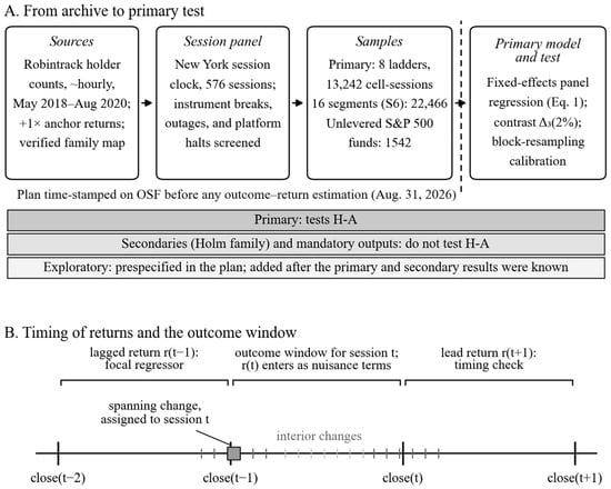
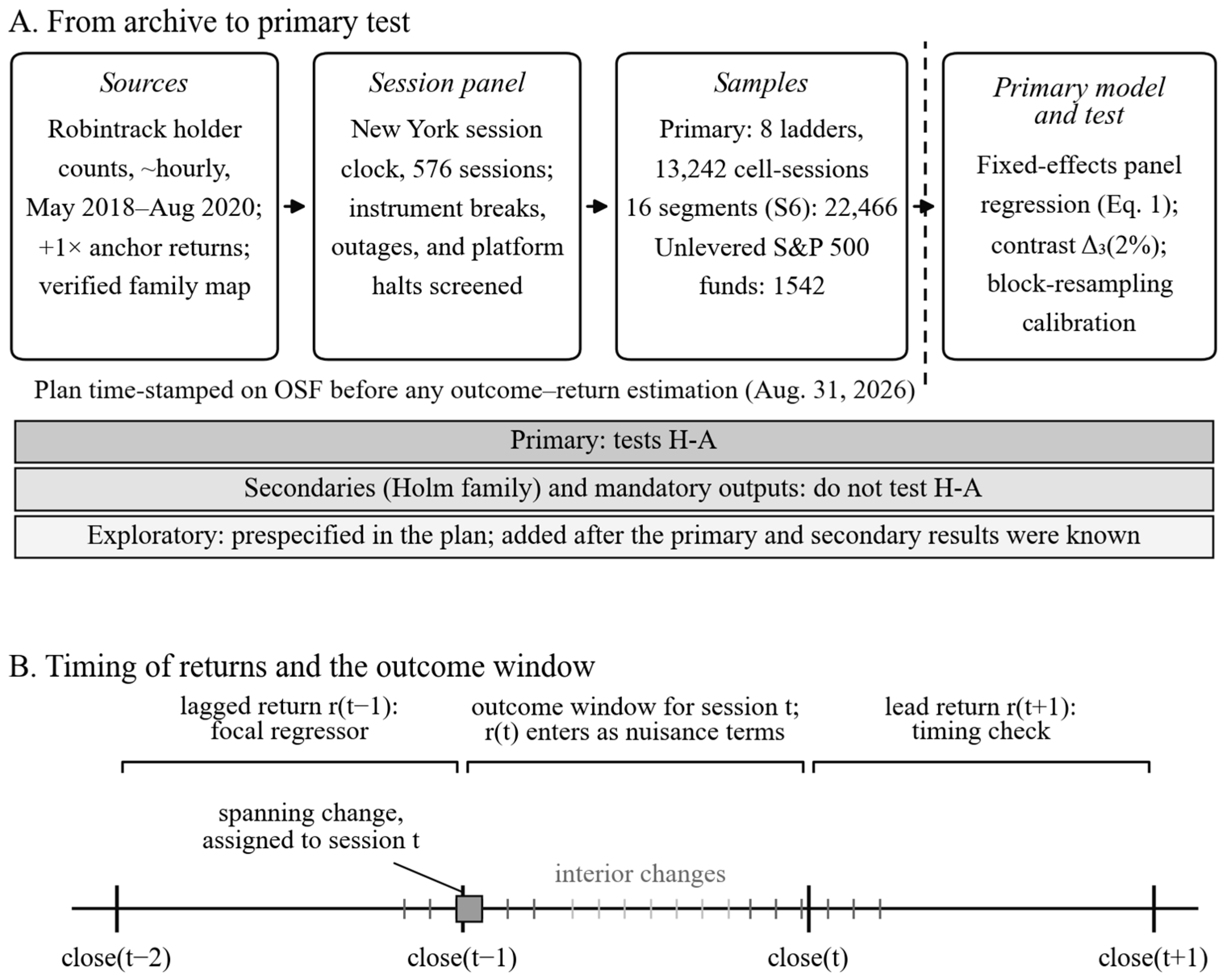
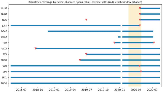
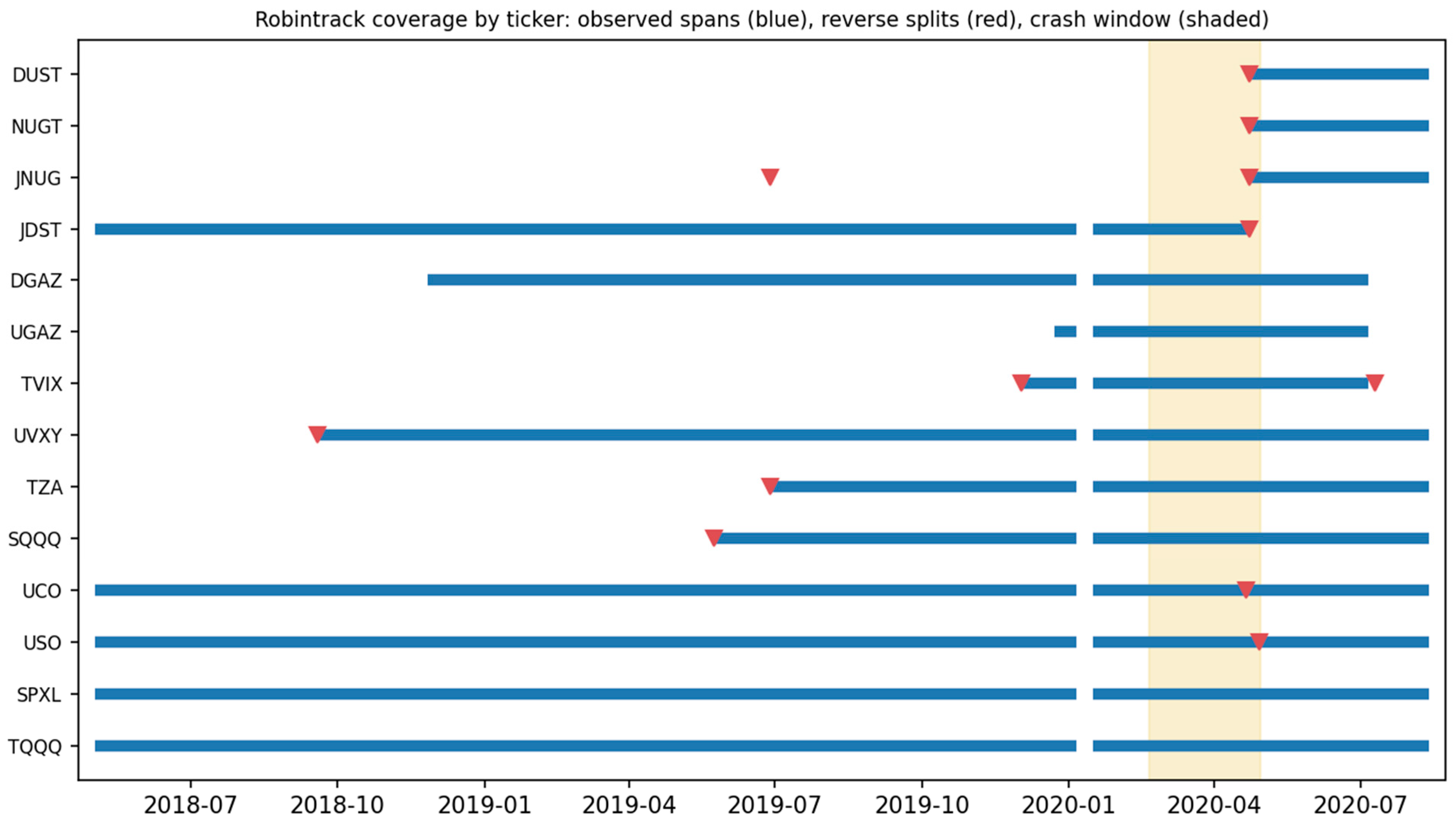
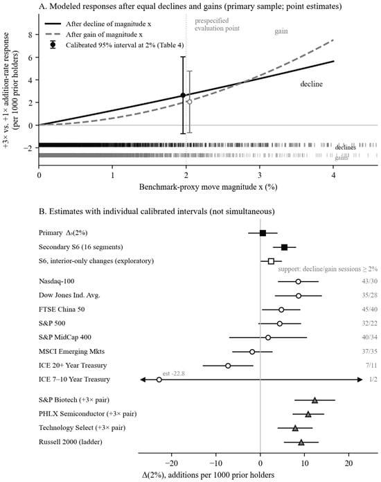

Disclaimer/Publisher’s Note: The statements, opinions and data contained in all publications are solely those of the individual author(s) and contributor(s) and not of MDPI and/or the editor(s). MDPI and/or the editor(s) disclaim responsibility for any injury to people or property resulting from any ideas, methods, instructions or products referred to in the content. |
© 2026 by the author. Licensee MDPI, Basel, Switzerland. This article is an open access article distributed under the terms and conditions of the Creative Commons Attribution (CC BY) license.