Abstract
To meet the control requirements of high precision and high robustness for peg-in-hole assembly tasks, an optimized control method for a peg-in-hole assembly task of a space manipulator is proposed to reduce the system disturbance caused by the change contact status during the assembly process. The first step is to build an equivalent stiffness model, which considers the structure and control characteristics of the space manipulator. Flexibility indices along the assembly direction are then created. On completion of the flexibility indices, the assembly configuration of the manipulator is optimized with the gain of the joint controller. After that, based on the sliding mode impedance control law, the disturbance of contact force is compensated using a zero-sum optimal control compensation strategy. Finally, the correctness and effectiveness of the control method are verified through simulation experiments. The results of the simulation experiments show that the contact force of the space manipulator can be precisely controlled by the method proposed in this paper. Compared with existing methods, the sudden change of contact force and the disturbing force of the base are reduced by 90% and 54%, respectively. A control method of the space manipulator for a peg-in-hole assembly task considering the equivalent stiffness optimization is proposed, which effectively reduces the influence of disturbance caused by contact collision and improves the control robustness of peg-in-hole assembly tasks.
1. Introduction
Deep space exploration and on-orbit service are major research projects in China’s space exploration. The development of related technologies will directly affect the implementation of China’s future space exploration plans and the deployment of related space strategies. During deep space exploration and on-orbit services, there are a lot of heavy and complex space assembly tasks to be completed, such as the dismantling and reorganization of abandoned satellites on-orbit and the construction of space solar power plants [1], the construction of the survey telescope [2], the construction of the Ultra-Large Aperture On-orbit Assembly Space Telescope [3,4], and the automated construction of the remote exploration base [5,6]. These tasks inevitably require space manipulators to complete inserting and screwing actions, which all belong to the peg-in-hole assembly task. As a typical inserting task, the peg-in-hole assembly task is representative of on-orbit operation tasks such as space unit replacement and equipment installation. Therefore, it is of great significance to study the peg-in-hole assembly technology of space manipulators.
When a space manipulator interacts with the environment, a small planning error may cause the object gripped by the manipulator to break away from the contact surface or produce excessive contact force. Unfortunately, there are usually errors in the position data during the assembly process. For example, the pose obtained by computer vision may have an error of ±6 mm [7,8]. The author once studied the pose estimation based on 3D point cloud in an area of 1 m2, and the maximum error was about 8 mm. To solve this problem, on the one hand, a hole search operation is required to find the specific position of the hole before the plug-in process (Figure 1). On the other hand, a compliance control method is needed to adjust the relationship between the position of the end of the manipulator and the contact force.
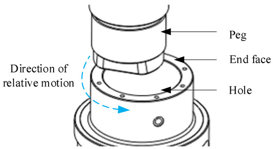
Figure 1.
Schematic diagram of peg-in-hole.
The compliance control method mainly includes hybrid position-force control and the impedance control method [9]. Chen [10] proposed a peg-in-hole assembly algorithm for robotic astronauts based on hybrid position-force control. Wu [11] studied the precision peg-in-hole assembly method of industrial manipulators based on hybrid position-force control. These algorithms are not of interest in this study because they switch between force and position control and need to identify the environmental parameters in real time to adjust the direction of the force. As a result, it is difficult to actualize fully compliant behavior. On the other hand, the impedance control [12] is successful when the manipulator is in free space and also when it is in contact with the environment. Thus, it can also be used in cases of unknown environments. Although the sensorless force controller has various advantages, its accuracy has difficulty meeting the requirements of assembly tasks [13,14], so this paper does not pay attention to these methods.
At the end of the hole search operation and the beginning of the plug-in process, the contact state of the assembly changes. It results in a sudden change in the contact force at the manipulator’s end, further causing disturbance of the base. It is likely to cause the vibration of the spacecraft structure and the instability of the attitude and orbit control system. More seriously, it may even damage the force sensor and other precision instruments due to the contact force amplitude exceeding the range and further damaging the space manipulator. Therefore, how to reduce the sudden change of contact force and suppress the disturbance of the base has become the key to the success of the peg-in-hole assembly task.
Restricted by launch conditions, the space manipulator exhibits significant flexibility due to its lightweight features. The flexibility of its joints and links is mapped to the operating space through the kinematics model of the manipulator, resulting in weak equivalent stiffness at the end of the space manipulator, which changes continuously with the change of configuration. This provides ideas for suppressing the sudden change of contact force and the disturbance of the base caused by it. That is, the manipulator can obtain better flexibility by optimizing the equivalent stiffness of the end so as to suppress the disturbance at the moment of contact collision and enhance the system’s robustness. Qu et al. integrated the stiffness model of each influencing factor into the overall stiffness model of the manipulator through the principle of superposition [15]. Hui et al. used the equivalent stiffness model to compensate for the deformation of the manipulator in the process of controlling the cutting force to improve the trajectory accuracy [16]. Jiao et al. proposed an optimization method based on the optimal equivalent stiffness, which can avoid the singularity and the limit of joint angles while obtaining an operating posture with better equivalent stiffness [17]. Lin et al. established the equivalent stiffness map of the end of the manipulator in the workspace to select the optimal position and determine the posture of the end through the deformation estimation index [18]. Qu et al. designed the fitness function based on the semi-axial length of the equivalent stiffness ellipsoid and used the Genetic Algorithm to optimize the pose of the 7-DOF redundant manipulator [19]. Tian et al. used the Rayleigh quotient to evaluate the stiffness performance of the manipulator and obtained the optimal configuration of the entire workspace with the Genetic Algorithm method [20]. However, there are specific problems with the build of equivalent stiffness model in the above studies. One of these is that they only considered the joint flexibility of the manipulator from the perspective of the structure’s inherent stiffness. Another is that they used the configuration as a decision variable for relevant analysis and optimization. For space manipulators performing assembly tasks, a compliance controller is required to obtain appropriate contact force. Control gain is an essential factor that causes the weak equivalent stiffness and the changing characteristics with the configuration of the end of the manipulator. Therefore, the effect of the control gain on the equivalent stiffness cannot be ignored.
During the process of peg-in-hole tasks, the sudden change in contact force can be regarded as the disturbance of the environment to the space manipulator system. By optimizing the equivalent stiffness of the space manipulator, the disturbance can be reduced to control the sudden contact force within the sensor range. However, the actual value of the contact force still has a significant sudden change compared with the expected value, which does not meet the accuracy requirements of the contact force control during peg-in-hole assembly. In the previous research on compliance control, Christian [21,22] proposed a control strategy that unified impedance control and admittance control based on a hybrid systems framework to improve the stability and performance characteristics of interaction controllers. CAESAR [23] was LWR3′s consistent continuation in the development of a force/torque-controlled robot system, which allowed the required stiffness setting range to be reduced to zero. Li et al. proposed a fuzzy sliding mode impedance controller to solve the problem of low robustness due to the uncertainty and disturbance of the manipulator or the environment [24]; Xiao realized autonomous peg-in-hole assembly by designing fuzzy rules to adjust impedance control parameters, but it requires professionals to refine and summarize the experience of adjusting parameters based on a large number of experiments [25]. Duan et al. designed an adaptive variable impedance model to achieve the trajectory tracking of the dual manipulator subject to external disturbance [26]; based on the collision model and the extended Kalman filter to estimate the environmental stiffness online, Roveda [27] proposed a discrete controller to realize the gain of the adaptive controller. Sadeghian et al. proposed a disturbance observer based on task error detection and conducted a disturbance force detection experiment on the KUKA LWR4 lightweight manipulator [28]; Jia et al. realized the impedance control of unknown disturbance in the nullspace of robotic astronauts by designing a disturbance observer [29]. Dong et al. designed a decentralized robust zero-sum optimal controller for a double-joint reconfigurable robot to realize disturbance compensation in an uncertain environment [30], inspiring this paper’s research. However, the decentralized control system compensates for disturbance in the joint space of the double-joint reconfigurable robot. So, its results cannot be directly applied to the peg-in-hole assembly in on-orbit operation tasks.
To sum up, the above research mainly has the following shortcomings: (1) Some researchers only considered the structural flexibility in the modeling and analysis of the equivalent stiffness of the manipulators but did not consider the influencing factors of the control method, which leads to the insufficient model of the equivalent stiffness. (2) Other researchers tuned the control parameters by estimating the environment stiffness in their work but did not consider the structural stiffness of the manipulator. However, the structural stiffness of the space manipulator may be much smaller than the environmental stiffness. (3) The existing research on impedance control have limitations when applied to space assembly tasks: The controller based on the hybrid systems framework needs to switch the control law frequently; designing fuzzy rules requires researchers to generalize on the basis of a large number of experiments; the stiffness estimation based on the extended Kalman filter leads to insufficient control accuracy; and controllers based on disturbance observers require accurate dynamics models.
Aiming at the above problems, in order to ensure the accuracy and robustness of the peg-in-hole assembly control, a control method of a space manipulator for peg-in-hole assembly tasks considering equivalent stiffness optimization is proposed in this paper. This method can reduce the sudden change in contact force and suppress the disturbing force of the base by determining the appropriate manipulator’s configuration and control gain. It improves the accuracy and robustness of peg-in-hole assembly control.
The research in this paper possesses the following traits:
- By combining the structure and control characteristics of the space manipulator, the controller parameters and configuration are introduced into the equivalent stiffness optimization process of the manipulator.
- By combining the advantages of the sliding mode control method, an impedance control law based on the result of equivalent stiffness optimization is deigned, and the zero-sum game is introduced to compensate for the interference caused by contact collision.
The rest of the paper is composed of five chapters. In the second chapter, the stiffness model of space manipulator is built. In the third chapter, the stiffness optimization method for peg-in-hole assembly is presented. In the fourth chapter, the sliding mode impedance control based on disturbance compensation is designed. In the fifth chapter, the simulation experiment and analysis are carried out. Finally, the conclusions are drawn.
2. Stiffness Modeling of Space Manipulator
2.1. Kinematics and Dynamics Model
In this section, a brief review of the kinematics and dynamics model of space manipulators is presented. The kinematics equations and dynamics equations of the space manipulator studied in this paper have general forms. Equations (1)–(3) are the position-level kinematics equation, the velocity-level kinematics equation, and the Cartesian space dynamics equation of the space manipulator, respectively:
where is the transformation matrix of two adjacent coordinate systems; , , , are functions of joint angle ; is the number of joints; (abbreviated as ) is the Jacobian matrix for the space manipulator; is the generalized operating force vector; are the Cartesian space inertia term and the Coriolis force term; is the end contact force in the Cartesian space of the space manipulator; and is the contact force disturbance term.
2.2. Equivalent Stiffness Model
Once the kinematics and dynamics models are obtained, the equivalent stiffness model can be created. The equivalent stiffness of the space manipulator is affected by the structural stiffness (joint stiffness and link stiffness) and control stiffness. The stiffness can be expressed as the inverse matrix of flexibility. For the joint flexibility, the differential motion vector of the link coordinate system can be obtained by calculating the bending and torsion deformation caused by the external load of the joint. For the flexibility of the link, the differential motion vector of the link coordinate system can be obtained by calculating the stretching, bending, and torsion deformation of the link. By analyzing the differential motion of the joint and link subjected to external forces, the flexible deformation of the end of the manipulator can be obtained. Then, the flexibility matrix can be obtained. For the control flexibility, it can be obtained by the joint controller gain and the Jacobian matrix.
2.2.1. Joint Flexibility
When the joint is subjected to an external load, it will produce bending deformation and torsion deformation. The differential motion of the link coordinate system caused by deformation is shown in Figure 2. The amount of deformation can be calculated by Equation (4) as follows:
where is the joint angle error caused by the torsional deformation of joint , is the torsional stiffness coefficient of joint , is the torque received by the joint , and are the differential rotation caused by the bending deformation of joint , is the bending stiffness coefficient of the joint , and and are the bending moment of the joint .
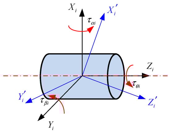
Figure 2.
The differential motion of the joint coordinate system is caused by joint deformation.
It can be seen from the differential motion that the end deformation caused by the torsion of the space manipulator joint and the end deformation and caused by the bending can be expressed as:
where represents the Jacobian matrix that maps the bending deformation of the joint space to the operation space, which can be abbreviated as and , respectively. The joins of the manipulator in this paper are all rotating joints, hence, the i-th column of and can be expressed as:
According to the duality principle, the static equivalent joint torque can be obtained from the external force at the manipulator’s end:
From Equations (4)–(6), the deformation of the end of the space manipulator caused by joint deformation can be obtained as:
where , are the diagonal matrices formed by and , respectively. Since the stiffness of each joint is not zero, these two matrices have inverse matrices.
When the joint deformation is minimal, the total deformation of the end can be expressed by Equation:
where , where represents the flexibility of the joint at the end of the space manipulator.
2.2.2. Link Flexibility
When force analysis is carried out on a link , it is regarded as a cantilever beam with a fixed head and a free end. A coordinate system is established at the end of the link. The origin of the coordinate system is at the intersection of the end section and the axis. Before the deformation of the link, each coordinate axis of is in the same direction with . As shown in Figure 3, the components of the force on the end of the link along the X, Y, and Z directions of are , , and , respectively, and the components of the torque on the end of the link along three axes are , , and , respectively.
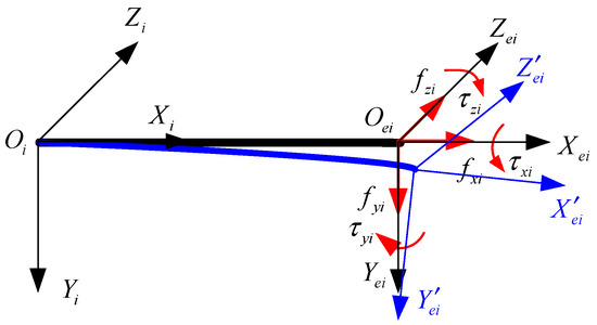
Figure 3.
The differential motion of the link coordinate system is caused by link deformation.
The differential motion vector of the coordinate system after deformation can be derived based on the analysis of the extension, bending, and torsion deformation of the link caused by the external force and torque as follows:
where is the length of the link and , , and are the tensile stiffness, bending stiffness, and torsional stiffness of the link, respectively.
It can be seen from the differential motion that the six-dimensional deformation caused by the stretching, bending, and torsion of the link can be expressed as:
where represent the Jacobian matrix where the deformation of the link is mapped from the joint space to the Cartesian space, abbreviated as , , and , and the -th column can be expressed as:
Under static conditions, according to the duality principle, the equivalent force of the link can be obtained from the external force at the end of the space manipulator as follows:
According to Equations (9)–(11), the deformation of the terminal of the space manipulator caused by the deformation of links can be obtained as:
where , , , , and .
When the link deformation is minimal, the total deformation at the end can be expressed as:
where indicates the flexibility of the links at the end of the space manipulator, and its expression is shown as in Equation (14):
2.2.3. Control Flexibility
It is defined that the control gain of the -th joint is and . The error of each joint caused by the joint torque can be obtained by Equation (15):
Thus, the pose error of the end of the manipulator generated by external influence is:
where represents the control flexibility at the end of the space manipulator.
In summary, the total deformation at the end of the space manipulator is:
where denotes the flexibility matrix of the end of the space manipulator, revealing the linear relationship between the external force and the endpoint deformation . The inverse matrix of represents the equivalent stiffness matrix at the end of the space manipulator.
The above is the equivalent stiffness model with more comprehensive factors. The analysis and optimization will be carried out in the next section.
3. Stiffness Optimization Method for Peg-in-Hole Assembly
Before optimizing the stiffness of the space manipulator, the corresponding evaluation index must be established.
3.1. Task Direction Flexibility
The aforementioned space manipulator end flexibility matrix is divided into four sub-matrices as follows:
where denotes the position error under the action of unit force, that is, the position flexibility; represents the attitude error under the unit torque, that is, the attitude flexibility; and denote the attitude coupling error under the action of a unit force.
The positional flexibility ellipsoid is designed as:
where , , and are the singular values of the matrix . is defined along the Z-axis of the space manipulator tool coordinate system to satisfy Equation (19) as the task direction flexibility of the peg-in-hole assembly. denotes the end position error under unit force in the task direction. It can be found that the larger the , the smaller the contact force generated by the unit error of the end of the space manipulator. Thus, can be optimized to suppress the sudden change in the contact force during the assembly process.
3.2. Optimization
For the peg-in-hole assembly task with determining the target pose, it is necessary to select the appropriate controller gain and configuration in the joint space to optimize the equivalent stiffness of the space manipulator. The optimization problem can be described as follows:
The Particle Swarm Optimization algorithm is used to solve the optimization problem described by Equation (20). For a manipulator with degrees of freedom, the dimension of the search space is . The decision variables of the algorithm can be designed as:
where .
If and are used to denote the position and velocity of the -th particle at step , and are used to denote the individual historical optimal solution and the group historical optimal solution of the -th particle at step , respectively. Then, the velocity and position update formula can be obtained by the following equation:
where is called the inertia factor, which denotes the degree of dependence of the particle on the initial value, that is, the ability to explore the global solution space; denotes the cognitive factor; is randomly distributed on the interval ; denotes the social factor; and is randomly distributed on the interval . and jointly determine the degree of dependence of the particle on the individual historical optimal solution. and jointly determine the degree of dependence of the particles on the optimal solution of the group.
This paper optimizes the configuration in the null space ( has a null space mapping matrix at ). It is assumed that the block matrix . Equation (23) is used to map to the null space of the space manipulator as follows:
where denotes identity matrix of order . Thus, the particle swarm velocity and position update formula is:
where is the constraint factor, which denotes the degree of inheritance of the speed of the current step update by the particles. The above parameters can be adjusted according to the different needs of the specific optimization problem.
During the optimization process, the velocity and position of the particles are continuously updated according to Equation (24). When the speed of each particle is zero and the position does not change or the algorithm reaches the maximum number of iterations, the calculation is terminated. The historical optimal solution of the group at this time is the final value of the decision vector. The decision vector is equally divided into two groups to obtain the optimized configuration and controller gain.
4. Sliding Mode Impedance Control Based on Disturbance Compensation
4.1. Sliding Mode Impedance Control
The impedance model is designed as follows:
where , , and denote the actual pose, velocity, and acceleration of the space manipulator in the working space, respectively; , , and denote the desired trajectory, desired speed, and acceleration of the space manipulator in the workspace, respectively; , , and are the mass, damping, and stiffness coefficients, respectively; and . The impedance control law can be designed according to Equation (25):
where .
The sliding mode function is designed as follows:
where is a positive definite diagonal matrix. Equation (26) is introduced into the sliding mode control mode, and the sliding mode control mode is designed considering Equation (3) as:
where and .
4.2. Disturbance Compensation
If the disturbance caused by the sudden change of contact force is regarded as an input of a control system, then the robust control problem can be transformed into a two-person zero-sum optimal control problem. is assumed as:
where and are symmetric positive definite constant matrices, and is a known normal number. The continuously differentiable performance index is defined as:
Based on performance indicators, the local Hamiltonian equation is defined as:
where .
The goal of the zero-sum game is to find a set of optimal control sequences, and , that satisfy the relationship of Equation (32):
When and execute their respective optimal control sequences, it can be considered that the saddle point of the two-person zero-sum game problem is obtained. At this time, the local optimal performance index is:
According to Equations (31) and (33), the HJI equation can be obtained as:
The solution and , satisfying Equation (34), should have the following form [31]:
The BP neural network is used to approximate the performance index, and the hyperbolic tangent function is selected as the activation function. The ideal neural network can be expressed as:
where denotes the unknown neural network weight, and denotes the neural network approximation error. Thus, the gradient of the performance index can be expressed as:
Equation (37) is substituted into Equation (31), which is then:
where is the approximation error. Thus, the output of the actual neural network is:
where is the estimated value of the weight . Thus, the approximation to the Hamiltonian equation is:
The residual function is created according to the steepest gradient descent method:
Thus, the renewal law of can be expressed as:
where denotes the learning rate.
Thus, can be obtained by combining Equations (35) and (39):
The sliding mode control law, by substituting Equation (43) into Equation (28), can be rewritten as:
5. Test and Analysis
To validate the control method proposed in this paper, three comparative stimulations on the space manipulator are designed. The first experiment used the existing control method [29] with disturbance observers but no optimized configuration and control parameters. The second experiment used the existing impedance control method with optimization of configuration and control parameters. The third experiment carries out the control algorithm proposed in this paper based on stiffness optimization and disturbance compensation.
5.1. Subject
The subject of the three experiments is a 7-DOF space manipulator. Figure 4 shows the space manipulator and its Denavit–Hartenberg (DH) model with a coordinate system. Table 1 shows the kinematic parameters of the space manipulator. The mass parameters are shown in Table 2, and the inertia tensor can be obtained from Table 2. The connecting rod is made of aluminum. The diameters of link 3 and link 4 are 96 mm and 70 mm, respectively, and the wall thickness is 5 mm.
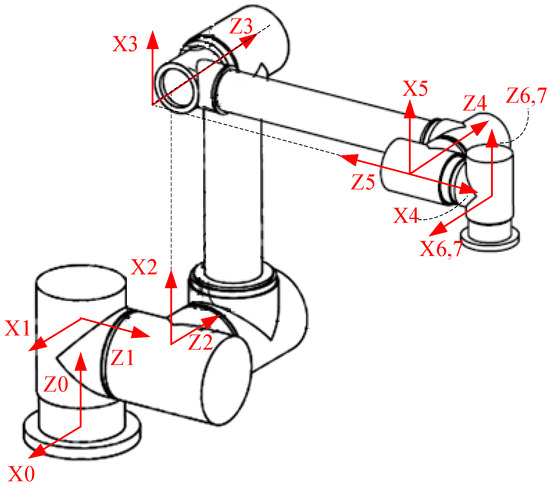
Figure 4.
Space manipulator and its coordinate systems.

Table 1.
Kinematic parameters of the space manipulator.
Table 2.
Inertial parameters of the space manipulator.
The base coordinate system of the space manipulator coincides with the world coordinate system, and its initial configuration is . The end tool clamps a peg with a mass of 5 kg to move from to . Restricted by the accuracy of the calibration of the vision sensor and the algorithm, there is an error of in . The motion trajectory of the space manipulator adopts the trapezoidal speed planning method with arc transition, the total planning time is , and the planning step length is . The control frequency is 100 Hz, and the measurement frequency is 1000 Hz.
5.2. Experiments
At the beginning of the experiments, the space manipulator clamped the peg to move linearly along the Z direction of the coordinate system. After the shaft is in contact with the end face of the hole, it enters the hole searching stage and moves along the vortex line, as shown in Figure 5. The contact force between the shaft and the end face of the hole is maintained at . After finding the hole, the space manipulator moves in a straight line through the hole. The contact forces mode is obtained according to the Hertz theory, and the simulation details of the environment are shown in the literature [32]. An error of 5% is added to the dynamics parameters to simulate its uncertainties. Matlab and its Robotics ToolboxCorke (Release 10) are used to simulate and verify the proposed method.
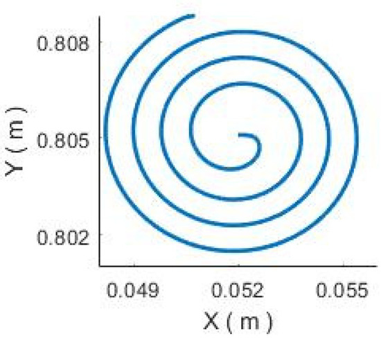
Figure 5.
The searching trajectory of the hole.
In experiment 1, the existing control method [29] was used, and the configuration and control parameters were not optimized. The simulation results are shown in Figure 6 and Figure 7. It can be seen that the hole searching phase ends at about the 4th second, and the peg loses contact with the hole and then collides. At this time, the contact force becomes 0 N and then abruptly reaches the peak value of 114 N. At the moment of collision, the peak disturbance force of the base comes 1086 N. In a practice project, such a large contact force can easily exceed the 100 N range of the sensor, which will affect the accuracy of the data and even damage the sensor. The tremendous disturbing force of the base will also cause massive interference to the attitude and orbit control of the base spacecraft.
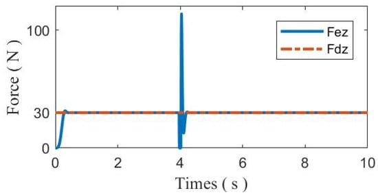
Figure 6.
The contact force between shaft and hole in experiment 1.
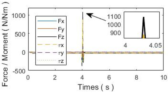
Figure 7.
Disturbance of the base in experiment 1.
In experiment 2, the existing impedance control method was used, and the configuration and control parameters were optimized. The number of the particle population is 50, the inertia factor is , , and the maximum iteration is 100 times. The convergence process and optimization results are shown in Figure 8. Before optimization, the joint controller gain is ( is 7 identity matrix) and the controller gain after optimization is . The optimized configuration is . The simulation results are shown in Figure 9 and Figure 10. It can be seen that due to the optimization of the manipulator’s configuration and controller gain, the peak contact force at the moment of contact collision drops to 77 N, which is 47% lower than that in Experiment 1. The peak disturbance force of the base is 534 N, and the decrease is 51%.
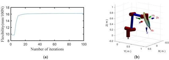
Figure 8.
The process and result of optimization. (a) Convergence process. (b) The optimized configuration and flexibility ellipsoid.
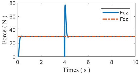
Figure 9.
The contact force between shaft and hole in experiment 2.
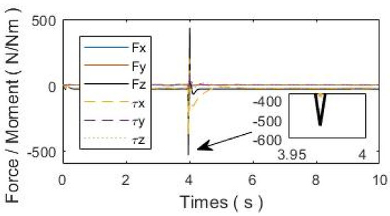
Figure 10.
Disturbance of the base in experiment 2.
In experiment 3, the control algorithm designed in this paper is used based on stiffness optimization and disturbance compensation. The BP neural network structure is set to 3-6-1, and the initial weight is randomly assigned within the range of . , , , and are all unit arrays, and . The neural network is trained up to 1000 times. The initial learning rate is , and each training decrements by 0.001, and , , , , , . The simulation results are shown in Figure 11 and Figure 12. It can be seen that due to the compensation based on the zero-sum optimal control algorithm, the peak value of the contact force is 38N, which is a 90% drop compared to experiment 1.

Figure 11.
The contact force between shaft and hole in experiment 3.
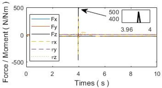
Figure 12.
Disturbance of the base in experiment 3.
A comparison between the experiments without and with the control algorithm proposed in this paper is shown in Table 3. It can be seen that the peg-in-hole assembly control method of the space manipulator proposed in this paper can effectively reduce the sudden change in contact force caused by collision and can suppress the disturbing force of the base by comparing the results of three experiments. The disturbance caused by the change of contact status during the assembly process is reduced to meet the control requirements of high precision and high robustness for peg-in-hole assembly tasks performed by a space manipulator.
Table 3.
The comparison between the experiments.
6. Conclusions
Based on the structure and control characteristics of the space manipulator, a space manipulator peg-in-hole assembly control method considering the optimization of equivalent stiffness is proposed in this paper. Compared with the existing compliance control method, the contributions of this paper mainly include the following points: (1) the method proposed in this paper designs the sliding mode impedance control law based on establishing and optimizing the equivalent stiffness; (2) this paper designs the optimal compensation term for the contact disturbance; (3) the methods proposed in this paper effectively reduce the sudden change in contact force caused by collision and can suppress the disturbing force of the base while controlling the contact force at the end of the space manipulator, thereby improving the accuracy and robustness of the peg-in-hole assembly control. In the later period, the dynamic coupling characteristics of flexible base and manipulator will be further taken into consideration for the multi-arm space robot performing the on-orbit assembly task of large trusses, and the coordinated control method of peg-in-hole assembly under the coupling vibration of multi-arm space robot will be studied.
Author Contributions
Conceptualization, G.P., Q.J. and G.C.; software and validation, G.P.; formal analysis, G.P.; resources, T.L. and C.L.; writing—original draft preparation, G.P.; writing—review and editing, G.P. and Q.J.; visualization, G.P. and G.C.; supervision, G.C. All authors have read and agreed to the published version of the manuscript.
Funding
This study was co-supported by the National Natural Science Foundation of China (No. 51975059 and No. 61802363), and State Administration of Science Technology and Industry for National Defense (No. HTKJ2019KL502012), and the Science and Technology Foundation of State Key Laboratory (No. 19NY1208).
Institutional Review Board Statement
Not applicable.
Informed Consent Statement
Not applicable.
Data Availability Statement
Not applicable.
Acknowledgments
The authors would like to acknowledge Huang Zeyuan, Fei Junting, Wang Ruiquan, Sun Fenglei, and the Key Laboratory of Space robotics, Ministry of Education for their help and expertise.
Conflicts of Interest
The authors declare no conflict of interest.
References
- Shi, Y.; Hou, X.; Rao, X.; Li, L.; Chen, T. Research on the Key Technology of Crawler Robot Orbiting on Space Solar Power Station. Space Electron. Technol. 2018, 15, 106–112. [Google Scholar] [CrossRef]
- Lu, S.; Zhang, T.; Zhang, X. Flat-field calibration method for large diameter survey mirror aperture splicing. Chin. Opt. 2020, 13, 1094–1102. [Google Scholar] [CrossRef]
- Hao, Z.; Jiang, Z.; Li, C.; Yang, F. Assembly Trajectory Planning of Space Telescope Sub-mirror Module Based on Time Optimal Control. IOP Conf. Ser. Mater. Sci. Eng. 2018, 439, 032077. [Google Scholar] [CrossRef]
- CIOMP. The Key Special Project of Strategic International Scientific and Technological Innovation Cooperation between CIOMP and the University of Surrey Was Officially Launched. Available online: http://www.ciomp.ac.cn/xwdt/zhxw/201711/t20171101_4882749.html (accessed on 28 May 2021).
- Pei, Z.; Liu, J.; Wang, Q.; Kang, Y.; Zou, Y.; Zhang, H.; Zhang, Y.; He, H.; Wang, Q.; Yang, R.; et al. Overview of lunar exploration and International Lunar Research Station. Chin. Sci. Bull. 2020, 65, 2577–2586. (In Chinese) [Google Scholar] [CrossRef]
- Feng, P.; Bao, C.; Zhang, D.; Yue, Q.; Qi, J.; Zuo, Y. Construction technology for lunar bases using lunar in-situ resources. Ind. Constr. 2021, 51, 169–178. [Google Scholar] [CrossRef]
- Huang, Y.; Chen, X.; Zhang, X. Kinematic Calibration and Vision-Based Object Grasping for Baxter Robot. In Proceedings of the International Conference on Intelligent Robotics and Applications, ICIRA 2016, Tokyo, Japan, 22–24 August 2016; Lecture Notes in Computer Science; Springer: Cham, Switzerland, 2016; Volume 9834. [Google Scholar] [CrossRef]
- Shah, G.A.; Polette, A.; Pernot, J.P.; Giannini, F.; Giannini, M. Simulated annealing-based fitting of CAD models to point clouds of mechanical parts’ assemblies. In Engineering with Computers; Springer: Cham, Switzertland, 2020. [Google Scholar] [CrossRef]
- Calanca, A.; Muradore, R.; Fiorini, P. A Review of Algorithms for Compliant Control of Stiff and Fixed-Compliance Robots. IEEE/ASME Trans. Mechatron. 2016, 21, 613–624. [Google Scholar] [CrossRef]
- Chen, G.; Wang, Y.; Jia, Q.; Sun, H.; Zhang, X. Hybrid Force and Position Control Strategy of Robonaut Performing Peg-in-Hole Assembly Task. J. Astronaut. 2017, 4, 410–419. [Google Scholar] [CrossRef]
- Wu, B.; Qu, D.; Xu, F. Industrial robot high precision peg in-hole assembly based on hybrid force/position control. J. Zhejiang Univ. Eng. Sci. 2018, 52, 379–386. [Google Scholar] [CrossRef]
- Hogan, N. Impedance control an approach to manipulation: Part I-theory, Part II-implementation, Part III-Application. J. Dyn. Syst. Meas. Control. 1985, 107, 1. [Google Scholar] [CrossRef]
- Roveda, L.; Piga, D. Robust state dependent riccati equation variable impedance control for robotic force-tracking tasks. Int. J. Intell. Robot. Appl. 2020, 4, 507–519. [Google Scholar] [CrossRef]
- Yang, C.; Ganesh, G.; Haddadin, S.; Parusel, S.; Albu-Schaeffer, A.; Burdet, E. Human-like adaptation of force and impedance in stable and unstable interactions. IEEE Trans. Robot. 2011, 27, 918–930. [Google Scholar] [CrossRef] [Green Version]
- Qu, M.; Wang, H.; Rong, Y. Static Stiffness Modeling and Experiments of Polishing Manipulator Arm. China Mech. Eng. 2017, 28, 2395–2401. [Google Scholar] [CrossRef]
- Hui, Z.; Wang, J.; Zhang, G.; Gan, Z.; Zhu, Z. Machining with flexible manipulator: Toward improving robotic machining performance. In Proceedings of the 2005 IEEE/ASME International Conference on Advanced Intelligent Mechatronics, Monterey, CA, USA, 24–28 July 2005; pp. 1127–1132. [Google Scholar] [CrossRef]
- Jiao, J.; Liao, W.; Tian, W.; Zhang, L.; Liu, S. A configuration optimizing method in robotic machining. Int. Robot. Autom. J. 2017, 3, 287–288. [Google Scholar] [CrossRef]
- Lin, Y.; Zhao, H.; Ding, H. Posture optimization methodology of 6R industrial robots for machining using performance evaluation indexes. Robot. Comput. Integr. Manuf. 2017, 48, 59–72. [Google Scholar] [CrossRef]
- Qu, W.; Hou, P.; Yang, G.; Huang, G.; Yin, F.; Shi, X. Research on the stiffness performance for robot machining systems. Acta Aeronaut. Astronaut. Sin. 2013, 34, 2823–2832. [Google Scholar] [CrossRef]
- Tian, Y.; Wang, B.; Liu, J.; Chen, F.; Yang, S.; Wang, W.; Li, L. Research on layout and operational pose optimization of robot grinding system based on optimal stiffness performance. J. Adv. Mech. Des. Syst. Manuf. 2017, 11, M22. [Google Scholar] [CrossRef] [Green Version]
- Ott, C.; Mukherjee, R.; Nakamura, Y. Unified impedance and admittance control. In Proceedings of the 2010 IEEE International Conference on Robotics and Automation, Anchorage, AK, USA, 3–8 May 2010. [Google Scholar] [CrossRef]
- Ott, C.; Mukherjee, R.; Nakamura, Y. A hybrid system framework for unified impedance and admittance control. J. Intell. Robot. Syst. 2015, 78, 359–375. [Google Scholar] [CrossRef]
- Beyer, A.; Grunwald, G.; Heumos, M.; Scheld, M.; Bayer, R.; Bertleff., W.; Brunner, B.; Burger, R.; Butterfaß, J.; Gruber, R.; et al. Caesar: Space robotics technology for assembly, maintenance, and repair. In Proceedings of the International Astronautical Congress, IAC, Bremen, Germany, 1–5 October 2018. [Google Scholar]
- Li, E.C.; Li, Z.M. The Robotic Force Tracking Based on Single Input Fuzzy Adaptive Controller. Adv. Mater. Res. 2011, 328–330, 2117–2120. [Google Scholar]
- Xiao, W. Research on Path Planning and Force Control of Peg-Hole Assembly Robot. Master’s Thesis, Xi’an University of Technology, Xi’an, China, 2018. [Google Scholar]
- Duan, J.; Gan, Y.; Chen, M.; Dai, X. Adaptive variable impedance control for dynamic contact force tracking in uncertain environment. Robot Auton. Syst. 2018, 102, 54–65. [Google Scholar] [CrossRef]
- Roveda, L.; Iannacci, N.; Molinari Tosatti, L. Discrete-time formulation for optimal impact control in interaction tasks. J. Intell. Robot. Syst. 2018, 90, 407–417. [Google Scholar] [CrossRef]
- Sadeghian, H.; Villani, L.; Keshmiri, M.; Siciliano, B. Task-Space Control of Robot Manipulators with Null-Space Compliance. IEEE Trans. Robot. 2014, 30, 493–506. [Google Scholar] [CrossRef]
- Jia, Q.; Xu, T.; Chen, G.; Sun, H.; Wang, Y. Coordinated Impedance Control of Robonaut Based on Disturbance Observer. Robot 2018, 6, 860–869. [Google Scholar] [CrossRef]
- Dong, B.; An, T.; Zhou, F.; Liu, K.; Li, Y. Decentralized robust zero-sum neuro-optimal control for modular robot manipulators in contact with uncertain environments: Theory and experimental verification. Nonlinear Dynam. 2019, 97, 503–524. [Google Scholar] [CrossRef]
- Aliyu, M.D.S. An approach for solving the Hamilton-Jacobi-Isaacs equation (HJIE) in nonlinear H∞ control. Automatica 2003, 39, 877–884. [Google Scholar] [CrossRef]
- Chen, G.; Liu, D.; Wang, Y.; Jia, Q.; Liu, X. Contact Force Minimization for Space Flexible Manipulators Based on Effective Mass. J. Guid. Control Dyn. 2019, 42, 1870–1877. [Google Scholar] [CrossRef]
Publisher’s Note: MDPI stays neutral with regard to jurisdictional claims in published maps and institutional affiliations. |
© 2021 by the authors. Licensee MDPI, Basel, Switzerland. This article is an open access article distributed under the terms and conditions of the Creative Commons Attribution (CC BY) license (https://creativecommons.org/licenses/by/4.0/).