Complementarity-Gap-Driven Adaptive Sequential Convex Programming for Reentry Trajectory Optimization

Abstract

To address the issue that existing penalty weight update strategies in the augmented Lagrangian multiplier method are disconnected from the optimality conditions and remain relatively sensitive to initial parameters, this paper proposes a complementarity-gap-driven adaptive sequential convex programming algorithm. The algorithm directly incorporates the complementarity slackness information from the KKT conditions into the parameter update laws. The defined complementarity slackness ratio and complementarity gap respectively measure the deviation of the current penalty intensity from the ideal multiplier level and the degree of departure from the complementarity slackness condition. Based on these two quantities, a bidirectional smooth update law for the penalty weight and a normalized gap update law for the multiplier are designed, which decouple the multiplier growth from the current multiplier magnitude. On this basis, a complete theoretical convergence framework is established, in which the monotonic bounded convergence of the Lagrange multiplier and the convergence of the slack variables and the complementarity gap are rigorously proved, and a conditional convergence theorem is given. Taking the reentry trajectory planning problem of a gliding vehicle as an example, numerical simulations are conducted with the initial penalty weight spanning five orders of magnitude. Simulation results demonstrate that the proposed algorithm converges rapidly and stably to the optimal solution satisfying the accuracy requirements under different initial weights, with the terminal position error stabilizing at 0.4–0.5 km, exhibiting favorable convergence accuracy. In addition, the stable convergence exhibited by the complementarity gap and the slackness radius validates the effectiveness and robustness of the complementarity-gap-driven adaptive update mechanism.

1. Introduction

When a reentry vehicle performs a mission subject to various constraints, the feasible flight trajectory may not be unique. It is therefore necessary to identify the optimal trajectory that satisfies the mission requirements, giving rise to the trajectory optimization problem. The vehicle trajectory optimization problem, also referred to as the optimal trajectory planning problem, seeks to determine an optimal or feasible trajectory under a set of constraints and can be classified as a constrained nonlinear optimal control problem (OCP). During flight, the vehicle must satisfy several types of constraints, including path constraints and terminal constraints. The presence of these constraints restricts the maneuverability of the vehicle to a certain extent. Under the premise of satisfying the aforementioned constraints, optimizing flight performance indicators—such as maximum range, maximum cross-range maneuver, minimum fuel consumption, and minimum flight time—has become a central focus of current research. Consequently, proper trajectory planning plays a crucial role in enhancing the maneuverability of reentry vehicles.

With the development of computer technology and various optimization algorithms, numerical methods for trajectory optimization have advanced considerably and have been widely applied in diverse scenarios. Depending on whether the performance index is optimized directly, numerical methods can be classified into direct methods [1,2] and indirect methods [3]. Indirect methods derive the first-order necessary conditions of the OCP based on Pontryagin’s maximum principle, transforming the original OCP into a Hamiltonian boundary value problem, whose optimality can be theoretically guaranteed. However, owing to the complexity of the theoretical derivation and the difficulty of accurately estimating the initial values of the adjoint variables, indirect methods are applied less frequently. In contrast, direct methods, which do not require the explicit derivation of optimality conditions, have been gradually popularized with the advancement of computer technology. Direct methods discretize the continuous-time OCP into a nonlinear programming (NLP) problem through parameterization and subsequently solve the NLP problem by numerical means. Nevertheless, typical reentry trajectory planning problems are highly non-convex, strongly nonlinear, and large in scale; their solution processes are usually time-consuming, and their convergence and optimality are difficult to guarantee [4], necessitating further verification of the obtained results.

In recent years, convex optimization methods have developed rapidly due to their global optimality, deterministic polynomial-time convergence, and low computational complexity [5], holding considerable potential for onboard applications. Acikmese et al. [6] applied convex optimization to the Mars pinpoint landing problem and, through lossless convexification (LCvx), transformed an OCP with non-convex control constraints into a second-order cone programming problem that can be solved efficiently. Lossless convexification typically employs techniques such as variable substitution, the introduction of slack variables to expand the feasible region, and convex approximation of constraints to convert non-convex problems into convex ones that are easier to solve [7,8]. However, lossless convexification cannot handle the more general and highly nonlinear non-convex constraints encountered in reentry trajectory planning problems. Sequential convex programming (SCP) provides a novel approach to addressing this challenge.

Sequential convex programming is an iterative method that transforms a non-convex optimization problem into a series of convex subproblems [9]. At each iteration of the SCP approach, a convex approximation of the original non-convex problem is constructed in the neighborhood of the current iterate through linearization or other convex approximation techniques, and the resulting sequence of convex subproblems is then solved iteratively using convex solvers. At present, SCP methods have been widely applied to spacecraft rendezvous and docking [10,11], orbit transfer [12,13], and vehicle reentry [14]. Meanwhile, SCP methods continue to be developed and refined in engineering practice [15,16]. To address the non-convexity arising from nonlinear dynamics, Mao et al. [17,18] proposed a Successive Convexification (SCvx) algorithm with favorable convergence properties. This algorithm convexifies the nonlinear dynamics through successive linearization and solves a convex subproblem at each iteration.

During the linearization process, certain approximation errors are inevitably introduced. Consequently, even if the original non-convex problem is feasible, the resulting convex subproblem may become infeasible due to these linearization errors, leading to the so-called artificial infeasibility problem. To address this issue, the SCvx algorithm employs slack variables and a trust region mechanism to resolve artificial infeasibility, thereby further enhancing the robustness of the algorithm [19]. If the slack variables are left unconstrained, excessively large slack variables would render the subproblem overly relaxed, causing it to lose the physical meaning of the original problem. Therefore, a strong penalty term on the slack variables is incorporated into the objective function, and the penalty coefficient is typically chosen to be relatively large [20]. Specifically, in most SCP methods, the product of a fixed penalty weight and the norm of the slack variables is added to the objective function [21,22], which then drives the slack variables toward zero to reduce the overall cost. As a result, the convergence behavior of SCP methods depends critically on whether the fixed penalty weight is properly selected; a weight that is either too large or too small can adversely affect convergence. Reference [23] proposed an adaptive penalty weight adjustment mechanism based on the augmented Lagrangian penalty method. This mechanism adjusts the penalty weight by monitoring the decay rate of the slack variables, thereby alleviating, to some extent, the difficulty of selecting a fixed weight. However, this mechanism has two limitations. First, the adjustment of the penalty weight depends solely on the decay rate of the slack variables and lacks a direct connection with the degree to which the Karush–Kuhn–Tucker (KKT) conditions (i.e., the first-order optimality conditions) are satisfied at the current iteration point. This means that even when the current solution is close to optimality, the weight may continue to grow because the slack variables have not yet fully converged, leading to over-penalization and numerical ill-conditioning. Second, the multiplier norm growth mechanism introduced in the Lagrange multiplier update and the penalty weight update mechanism are decoupled from each other, lacking information exchange and coordinated interaction. The stability and convergence of this open-loop adjustment strategy lack theoretical guarantees, and the strategy remains relatively sensitive to the choice of the initial penalty weight.

To address the above issues, this paper proposes a complementarity-gap-driven adaptive sequential convex programming (CGD-ASCP) method. Compared with existing approaches, the core distinction of CGD-ASCP lies in directly incorporating the complementarity slackness information from the KKT conditions as a feedback signal into the parameter update laws, thereby transforming the adjustment of the penalty weight and the multiplier from open-loop control into closed-loop correction based on the optimality conditions. Specifically, this paper defines two complementarity slackness metrics—the complementarity slackness ratio and the complementarity gap—which are used to evaluate the deviation between the penalty intensity and the ideal multiplier level, and the degree of constraint violation of the complementarity slackness condition, respectively. Based on these two metrics, a smooth bidirectional adjustment law for the penalty weight and a normalized gap update law for the multiplier are designed, achieving the following: (1) the multiplier growth is decoupled from the current multiplier magnitude, avoiding the dependence of weight growth on the multiplier magnitude; and (2) the penalty weight and the multiplier form a coordinated adjustment mechanism, simultaneously strengthening both the penalty and the multiplier feedback when the constraint violation increases, and synchronously stabilizing both when the constraints approach satisfaction. On this basis, a complete theoretical convergence framework is established, rigorously proving properties such as the monotonic bounded convergence of the multiplier, the convergence of the slack variables, and the convergence of the complementarity gap. Extensive numerical simulations are conducted on a gliding vehicle reentry trajectory planning problem with initial penalty weights spanning five orders of magnitude.

The main contributions of this paper can be summarized as follows: (1) a complementarity-gap-driven adaptive sequential convex programming method (CGD-ASCP) is proposed, which incorporates the KKT complementarity slackness information into the parameter update laws, uses the complementarity slackness ratio and the complementarity gap to drive the adaptive adjustment of the penalty weight and the multiplier, respectively, and achieves their coordinated closed-loop control, fundamentally distinguishing itself from existing open-loop or decoupled adjustment strategies; (2) a complete theoretical convergence framework for the algorithm is established, rigorously proving key properties such as the boundedness of the multiplier, the convergence of the slack variables, and the convergence of the complementarity gap; and (3) the robustness and computational efficiency of the algorithm are validated through a gliding vehicle reentry trajectory planning example, with the initial penalty weight spanning five orders of magnitude.

The remainder of this paper is organized as follows. Section 2 presents the mathematical formulation of the general nonlinear trajectory planning problem. Section 3 elaborates on the update strategy and parameter design of the CGD-ASCP algorithm and presents its theoretical convergence framework. Section 4 carries out numerical simulations for algorithm verification and comparative analysis. Finally, Section 5 summarizes the work of this paper.

2. Problem Formulation

2.1. Nonlinear Trajectory Planning Problem

A general reentry trajectory optimization problem is a continuous-time nonlinear optimal control problem, as shown in Equation (1).

Problem 1

$$\begin{array}{l}\min \hspace{0.33em}{J}_1=\phi (x(t_f),t_f)+{\displaystyle {\int }_0^{t_f}l}(x(t),u(t),t)\mathrm{d}t\\ \mathrm{s}.\mathrm{t}. \dot{x}(t)=f(x(t),u(t),t),\hspace{0.33em}\hspace{0.33em}\hspace{0.33em}x(0)=x_0\\ \hspace{0.33em}\hspace{0.33em}\hspace{0.33em}\hspace{0.33em}{s}_1(x(t),u(t),t)\le 0,\hspace{0.33em}\hspace{0.33em}\hspace{0.33em}{s}_2(x(t),u(t),t)=0\\ \hspace{0.33em}\hspace{0.33em}\hspace{0.33em}\hspace{0.33em}{\psi }_1(x(t_f),t_f)\le 0,\hspace{0.33em}\hspace{0.33em}\hspace{0.33em}{\psi }_2(x(t_f),t_f)=0\end{array}$$

(1)

where time $t\in {ℝ}_{++}$ is the independent variable. In this paper, the final time $t_f$ is free and should be optimized according to the mission. The state vector is $x:{ℝ}_{++}\to {ℝ}^{n_x}$ with dimension $n_x$; the control vector is $u:{ℝ}_{++}\to {ℝ}^{n_u}$ with dimension $n_u$. The initial state is $x_0\in {ℝ}^{n_x}$. The terminal cost function $\phi :{ℝ}^{n_x}\times ℝ\to ℝ$ depends on the terminal state and terminal time, i.e., on the mission requirements at the final target. The running cost function $l:{ℝ}^{n_x}\times {ℝ}^{n_u}\times ℝ\to ℝ$ depends on the evolution of states and controls over the entire time horizon. The right-hand side of the dynamic equation is $f:{ℝ}^{n_x}\times {ℝ}^{n_u}\times ℝ\to {ℝ}^{n_x}$. The path inequality constraints are given by $s_1:{ℝ}^{n_x}\times {ℝ}^{n_u}\times ℝ\to {ℝ}^{n_{s_1}}$, where $n_{s_1}$ is the number of path inequality constraints; the path equality constraints are given by $s_2:{ℝ}^{n_x}\times {ℝ}^{n_u}\times ℝ\to {ℝ}^{n_{s_2}}$, where $n_{s_2}$ is the number of path equality constraints. The terminal inequality constraints are ${\psi }_1:{ℝ}^{n_x}\times ℝ\to {ℝ}^{n_{{\psi }_1}}$, where $n_{{\psi }_1}$ is the number of terminal inequality constraints; the terminal equality constraints are ${\psi }_2:{ℝ}^{n_x}\times ℝ\to {ℝ}^{n_{{\psi }_2}}$, where $n_{{\psi }_2}$ is the number of terminal equality constraints.

The original Problem 1 is a continuous-time Bolza-type optimal control problem. Since computers can only handle finite-dimensional variables, it must first be discretized in the time domain when solving numerically. Commonly used discretization methods include the Euler method, the trapezoidal method, the fourth-order Runge–Kutta method, and pseudospectral methods. Regardless of the discretization method employed, the original continuous Problem 1 can be transformed into the following discrete form, i.e., Problem 2.

Problem 2

$$\begin{array}{l}\min \hspace{0.33em}{J}_2=\phi (x_N,N)+{\displaystyle \sum _{i=1}^{N}l}(x_i,u_i,i)\Delta t\\ \mathrm{s}.\mathrm{t}. F(x_i,u_i,x_{i-1},u_{i-1},\Delta t)=0,\hspace{0.33em}\hspace{0.33em}\hspace{0.33em}i=2,\dots ,N\\ \hspace{0.33em}\hspace{0.33em}\hspace{0.33em}\hspace{0.33em}{s}_1(x_i,u_i,i)\le 0,\hspace{0.33em}\hspace{0.33em}\hspace{0.33em}{s}_2(x_i,u_i,i)=0,\hspace{0.33em}\hspace{0.33em}\hspace{0.33em}i=1,\dots ,N\\ \hspace{0.33em}\hspace{0.33em}\hspace{0.33em}\hspace{0.33em}{x}_1=x_0\\ \hspace{0.33em}\hspace{0.33em}\hspace{0.33em}\hspace{0.33em}{\psi }_1(x_N,N)\le 0,\hspace{0.33em}\hspace{0.33em}\hspace{0.33em}{\psi }_2(x_N,N)=0\end{array}$$

(2)

where $N\in {\mathbb{N}}_{+}$ with $N\ge 2$ is the total number of discretization points, $x_i\in {ℝ}^{n_x}$ is the state variable at the $i$-th discretization point, $x_N\in {ℝ}^{n_x}$ is the state at the terminal point (final state), $u_i\in {ℝ}^{n_u}$ is the control variable at the $i$-th discretization point, $\Delta t:=t_f/(N-1)\in {ℝ}_{++}$ is the discrete time step, and $F$ is the algebraic constraint function obtained after discretizing the dynamics, whose specific form depends on the discretization method. For the trapezoidal discretization scheme, the explicit form of $F$ is given in Equation (3).

$$F_{\mathrm{trap}}\triangleq x_i-x_{i-1}-{\displaystyle \frac{\Delta t}{2}}(f(x_i,u_i,i)+f(x_{i-1},u_{i-1},i-1))=0$$

(3)

Although Problem 2 transforms the continuous-time optimization problem into a finite-dimensional one, it still retains the strongly nonlinear structure of the dynamic equations and constraints, which cannot be readily handled by general-purpose NLP solvers. To facilitate a unified description and subsequent linearization, the optimization variables are aggregated into a global vector, i.e., define $X:={[x_1^{\mathrm{T}},\cdots ,x_N^{\mathrm{T}},u_1^{\mathrm{T}},\cdots ,u_N^{\mathrm{T}},t_f]}^{\mathrm{T}}\in {ℝ}^n$ as the global optimization variable, where the total dimension is $n=(n_x+n_u)N+1$. Problem 2 can then be rewritten in the standard NLP form, i.e., Problem 3.

Problem 3

$$\begin{array}{l}{\min }_X\hspace{0.33em}{J}_3(X)=f(X)\\ \mathrm{s}.\mathrm{t}.\hspace{0.33em}\hspace{0.33em}\hspace{0.33em}h(X)=0,\hspace{0.33em}\hspace{0.33em}\hspace{0.33em}g(X)\le 0\end{array}$$

(4)

where $J_3:{ℝ}^n\to ℝ$, $f:{ℝ}^n\to ℝ$ is the objective function, $h:{ℝ}^n\to {ℝ}^{n_h}$ is the collection of all equality constraints, with the total number of equality constraints $n_h=n_x+(N-1)n_x+N\cdot n_{s_2}+n_{{\psi }_2}$; and $g:{ℝ}^n\to {ℝ}^{n_g}$ is the collection of all inequality constraints, with the total number of inequality constraints $n_g=N\cdot n_{s_1}+n_{{\psi }_1}$.

2.2. General Sequential Convex Programming Algorithm

Problem 3 is a high-dimensional NLP problem. Solving it directly would require a large amount of computation and cannot easily guarantee global optimality. The sequential convex programming (SCP) method approximates the original problem as a sequence of convex subproblems by linearizing the non-convex functions at each iteration, thereby significantly improving the solution efficiency. To ensure the validity of the linearization approximation and the convergence of the algorithm, the SCP method requires the following core assumptions: (1) the objective and constraint functions are at least once continuously differentiable; (2) the interior of the feasible set of each subproblem is non-empty; and (3) there exists at least one optimal point for the original problem [24]. The detailed assumptions and the verification that the reentry trajectory optimization problem addressed in this paper satisfies these conditions are presented in Section 3.3. Therefore, following the SCP approach, at the $k$-th iteration, Problem 3 is linearized around the current iterate $X^{(k)}$ via first-order Taylor expansion and transformed into a convex subproblem without relaxation variables, i.e., Problem 4.

Problem 4

$$\begin{array}{l}\min \hspace{0.33em}\hspace{0.33em}{J}_4={\nabla }^{\mathrm{T}}f(X^{(k)})(X-X^{(k)})\\ \mathrm{s}.\mathrm{t}. h(X^{(k)})+{\nabla }^{\mathrm{T}}h(X^{(k)})(X-X^{(k)})=0\\ \hspace{0.33em}\hspace{0.33em}\hspace{0.33em}\hspace{0.33em}\hspace{0.33em}g(X^{(k)})+{\nabla }^{\mathrm{T}}g(X^{(k)})(X-X^{(k)})\le 0\\ \hspace{0.33em}\hspace{0.33em}\hspace{0.33em}\hspace{0.33em}\hspace{0.33em}\Vert X-X^{(k)}{\Vert }_2\le {\delta }_X\end{array}$$

(5)

where ${\nabla }^{\mathrm{T}}f(X^{(k)})$ denotes the transpose of the gradient of $f(X)$ at the current iteration point $X^{(k)}$; ${\nabla }^{\mathrm{T}}h(X^{(k)})$ and ${\nabla }^{\mathrm{T}}g(X^{(k)})$ are the transposes of the Jacobian matrices of the equality constraints $h(X)$ and the inequality constraints $g(X)$ at $X^{(k)}$, respectively. The trust-region radius ${\delta }_X$ is introduced to confine the linearization of the global optimization variable $X$ within a neighborhood of $X^{(k)}$, thereby ensuring the validity of the linearization.

3. CGD-ASCP Method

3.1. Augmented Lagrange Multiplier SCP Method

Problem 4 constructs a locally convex approximation through linearization. However, when the reference point $X^{(k)}$ is far from the feasible region, the linearized equality constraints may not be satisfiable, causing the subproblem to be infeasible—a phenomenon known as artificial infeasibility introduced by linearization. To address this issue, Reference [25] introduces slack variables $\mathit{S}$ into the equality constraints to guarantee the existence of a feasible solution after linearization. Building upon this, Reference [23] incorporates an augmented Lagrangian multiplier framework, adding a penalty term ${\omega }_S{\delta }_S^2/2+\lambda {\delta }_S$ to the objective. Through the adaptive update of the multiplier $\lambda$, the slack variables gradually converge to zero, eventually restoring the feasibility of the original equality constraints. This yields a convex subproblem with slack variables and an augmented Lagrangian penalty, referred to as Problem 5.

Problem 5

$$\begin{array}{l}\min \hspace{0.33em}\hspace{0.33em}{J}_5={\nabla }^{\mathrm{T}}f(X^{(k)})(X-X^{(k)})+{\displaystyle \frac{1}{2}}{\omega }_S{\delta }_S^2+\lambda {\delta }_S\\ \mathrm{s}.\mathrm{t}. h(X^{(k)})+{\nabla }^{\mathrm{T}}h(X^{(k)})(X-X^{(k)})+S=0\\ \hspace{0.33em}\hspace{0.33em}\hspace{0.33em}\hspace{0.33em}\hspace{0.33em}g(X^{(k)})+{\nabla }^{\mathrm{T}}g(X^{(k)})(X-X^{(k)})\le 0\\ \hspace{0.33em}\hspace{0.33em}\hspace{0.33em}\hspace{0.33em}\hspace{0.33em}\Vert X-X^{(k)}{\Vert }_2\le {\delta }_X,\hspace{0.33em}\hspace{0.33em}\Vert S{\Vert }_2\le {\delta }_S\end{array}$$

(6)

Problem 5 restricts the slack variable $S$ within a range ${\delta }_S$ by introducing the relaxed trust-region constraint $\Vert S{\Vert }_2\le {\delta }_S$, and adds a penalty ${\omega }_S{\delta }_S^2/2+\lambda {\delta }_S$ to the objective function, where $\lambda \in ℝ$ is the Lagrange multiplier [26,27]. The above formulation uses only one Lagrange multiplier to penalize the overall constraint ${\delta }_S$ on the slack variables of all equality constraints, thereby avoiding the problem of excessively large slack variable sets that would arise if a multiplier were introduced for each equality constraint individually. Furthermore, by introducing the Lagrange multiplier, the ill-conditioning of the Hessian matrix and the associated numerical issues arising from the penalty weight tending to infinity in the case of using the $\Vert S{\Vert }_1$ penalty alone can be avoided [28].

The Lagrangian function of Problem 5 is given in Equation (7).

$$\begin{array}{l}L=f(X)+{\displaystyle \frac{1}{2}}{\omega }_S{\delta }_S^2+\lambda {\delta }_S+v^T(h(X^{(k)})+{\nabla }^{T}h(X^{(k)})(X-X^{(k)})+S)+\\ {\mu }_g^T(g(X^{(k)})+{\nabla }^{T}g(X^{(k)})(X-X^{(k)}))+{\mu }_1(\Vert X-X^{(k)}{\Vert }_2^2-{\delta }_X^2)-{\mu }_2{\delta }_X+\\ {\mu }_3(S^{T}S-{\delta }_S^2)-{\mu }_4{\delta }_S\end{array}$$

(7)

The KKT conditions of Problem 5 are expressed in Equations (8)–(15).

The optimality conditions are given in Equations (8) and (9).

$${\nabla }_{X}L=\nabla f(X)+\nabla h(X^{(k)})v+\nabla g(X^{(k)}){\mu }_g+2{\mu }_1(X-X^{(k)})=\mathbf{0}$$

(8)

$${\nabla }_{{\delta }_S}L={\omega }_S{\delta }_S+\lambda -2{\mu }_3{\delta }_S-{\mu }_4=0,\hspace{0.33em}\hspace{0.33em}\hspace{0.33em}{\nabla }_{S}L=v+2{\mu }_{3}S=\mathbf{0}$$

(9)

The primal constraints are given in Equations (10)–(12).

$$h(X^{(k)})+{\nabla }^{T}h(X^{(k)})(X-X^{(k)})+S=\mathbf{0}$$

(10)

$$g(X^{(k)})+{\nabla }^{T}g(X^{(k)})(X-X^{(k)})\le \mathbf{0}$$

(11)

$$\Vert X-X^{(k)}{\Vert }_2\le {\delta }_X,\hspace{0.33em}\hspace{0.33em}\hspace{0.33em}\Vert S{\Vert }_2\le {\delta }_S$$

(12)

The complementary slackness conditions are given in Equations (13)–(15).

$${\mu }_g\ge 0,\hspace{0.33em}\hspace{0.33em}\hspace{0.33em}{\mu }_1\ge 0,\hspace{0.33em}\hspace{0.33em}\hspace{0.33em}{\mu }_2\ge 0,\hspace{0.33em}\hspace{0.33em}\hspace{0.33em}{\mu }_3\ge 0,\hspace{0.33em}\hspace{0.33em}\hspace{0.33em}{\mu }_4\ge 0$$

(13)

$$\mathrm{diag}({\mu }_g)(g(X^{(k)})+{\nabla }^{T}g(X^{(k)})(X-X^{(k)}))=\mathbf{0}$$

(14)

$${\mu }_1\left(\Vert X-X^{(k)}{\Vert }_2^2-{\delta }_X^2\right)=0,\hspace{0.33em}\hspace{0.33em}\hspace{0.33em}{\mu }_2{\delta }_X=0,\hspace{0.33em}\hspace{0.33em}\hspace{0.33em}{\mu }_3(S^{T}S-{\delta }_S^2)=0,\hspace{0.33em}\hspace{0.33em}\hspace{0.33em}{\mu }_4{\delta }_S=0$$

(15)

The optimal solution to Problem 5 is denoted as $(X^{(k+1)},S^{(k+1)},{\delta }_S^{(k+1)})$, and the corresponding Lagrange multipliers are $v^{(k)},{\mu }_g^{(k)},{\mu }_1^{(k)},{\mu }_2^{(k)},{\mu }_3^{(k)},{\mu }_4^{(k)}$.

3.2. Complementarity-Gap-Driven Adaptive Update Strategy

The complementarity-gap-driven adaptive update strategy proposed in this paper includes update formulas for the penalty weight ${\omega }_S$, the Lagrange multiplier $\lambda$, the upper bound ${\delta }_S$ of the relaxed trust region for equality constraints, and the trust-region radius ${\delta }_X$ of the optimization variable $X$. Specifically, the iterative formula for ${\omega }_S$ is given in Equation (16).

$$\begin{array}{l}{\eta }^{(k+1)}=\min \left({\displaystyle \frac{\Vert v^{(k+1)}{\Vert }_2}{{\lambda }^{(k)}+ϵ}},{\eta }_{\max }\right)\\ {\eta }_{\mathrm{target}}^{(k+1)}={\eta }_{\mathrm{target}}^{\mathrm{final}}+({\eta }_{\mathrm{target}}^{\mathrm{init}}-{\eta }_{\mathrm{target}}^{\mathrm{final}})\exp \left(-(k+1)/T\right)\\ {\omega }_S^{(k+1)}={\omega }_S^{(k)}\cdot \min \left(\max \left({\left({\displaystyle \frac{{\eta }^{(k+1)}}{{\eta }_{\mathrm{target}}^{(k+1)}}}\right)}^p,{\tau }^{-1}\right),\tau \right)={\omega }_S^{(k)}\cdot \mathrm{sat}\left({\left({\displaystyle \frac{{\eta }^{(k+1)}}{{\eta }_{\mathrm{target}}^{(k+1)}}}\right)}^p,{\tau }^{-1},\tau \right)\\ {\omega }_S^{(k+1)}=\max \left(\min \left({\omega }_S^{(k+1)},{\omega }_{\max }\right),{\omega }_{\min }\right)\end{array}$$

(16)

In Equation (16), $\eta$ is the normalized ratio of the norm of the Lagrange multiplier $v$ corresponding to the equality constraints to the augmented Lagrange multiplier $\lambda$, which measures the relative magnitude of the multipliers, with ${\eta }_{\max }$ being its upper bound; ${\eta }_{\mathrm{target}}^{(k+1)}$ is the target value of $\eta$ at the $k+1$-th iteration, where ${\eta }_{\mathrm{target}}^{\mathrm{init}}$ and ${\eta }_{\mathrm{target}}^{\mathrm{final}}$ are its initial and final values, respectively; $T$ is the decay time constant controlling the decay rate; $p$ is the power exponent controlling the nonlinear response of the ratio; $\tau >1$ is the maximum step change factor; $\mathrm{sat}\left(x,a,b\right)=\min (\max (x,a),b)$ is the saturation function; and ${\omega }_{\min },{\omega }_{\max }$ are the lower and upper bounds of the penalty weight, respectively, used to avoid numerical ill-conditioning.

In Equation (16), $\eta$ combines the multiplier norm $\left|\right|v{\left|\right|}_2$ and the multiplier $\lambda$, indirectly linking the KKT conditions and reflecting the appropriateness of the current penalty strength. Compared with relying solely on the decay of ${\delta }_S$, it provides a more direct indication of the optimality condition. The target ${\eta }_{\mathrm{target}}$ is designed to be loose first and tight later, i.e., it decays from a large value to a small one. In the early stage, larger constraint violations are tolerated to avoid prematurely suppressing the objective function, while in the later stage the tighter target forces the constraints to be satisfied accurately, balancing convergence speed and solution accuracy. Furthermore, the saturation function limits the step-by-step change of the penalty weight to at most a factor of $\tau$, thereby avoiding oscillations that may be caused by fixed rate adjustments while achieving continuous adaptive bidirectional smooth regulation.

The iterative formula for the Lagrange multiplier $\lambda$ is given in Equation (17).

$$\begin{array}{l}ga{p}^{(k+1)}={\lambda }^{(k)}{\delta }_S^{(k+1)}-{(v^{(k+1)})}^T{S}^{(k+1)}\\ {\lambda }^{(k+1)}={\lambda }^{(k)}+{\beta }_{\lambda }{\omega }_S^{(k+1)}{\delta }_S^{(k+1)}+{\gamma }_{\mathrm{gap}}{\displaystyle \frac{ga{p}^{(k+1)}}{{\lambda }^{(k)}+\epsilon }}\end{array}$$

(17)

In Equation (17), gap is the complementary slackness residual, which measures the degree to which the current iteration point satisfies the complementary slackness condition; ${\beta }_{\lambda }$ is the weight coefficient for the contribution of the penalty term ${\omega }_S^{(k+1)}{\delta }_S^{(k+1)}$ to the multiplier update; ${\gamma }_{\mathrm{gap}}$ is the weight coefficient for the contribution of the normalized complementary slackness residual to the multiplier update. In Equation (17), the complementary slackness residual gap is divided by $\lambda +ϵ$ to achieve magnitude decoupling, so that the contribution of the $gap$ term matches the current magnitude of $\lambda$, making the growth of $\lambda$ more stable. Moreover, the definition of $gap$ directly measures the degree of deviation from the complementary slackness condition, and the direct feedback based on complementary slackness links the adjustment of $\lambda$ directly to optimality, which is more precise than relying solely on $\left|\right|v|{|}_2$. This update formula combines the explicit penalty term ${\beta }_{\lambda }{\omega }_S{\delta }_S$ with the normalized complementary slackness residual ${\gamma }_{\mathrm{gap}}\cdot gap/(\lambda +\epsilon )$, adding a closed-loop correction based on the KKT conditions while retaining the original penalty drive, thereby accelerating convergence and improving iteration robustness.

The update formula for the upper bound ${\delta }_S$ of the relaxed trust region for equality constraints is given in Equation (18).

$${\overline{\delta }}_S^{(k+1)}=\left\{\begin{array}{c}\min ({\overline{\delta }}_S^{(k)}\cdot {\delta }_{S,\mathrm{scale}},{\delta }_{S,\max }),{\delta }_S^{(k+1)}\ge {\theta }_S{\overline{\delta }}_S^{(k)}\\ \hspace{0.33em}\hspace{0.33em}\hspace{0.33em}\hspace{0.33em}\hspace{0.33em}{\overline{\delta }}_S^{(k)},\hspace{0.33em}\hspace{0.33em}\hspace{0.33em}\hspace{0.33em}\hspace{0.33em}\hspace{0.33em}\hspace{0.33em}\hspace{0.33em}\hspace{0.33em}\hspace{0.33em}{\delta }_S^{(k+1)}<{\theta }_S{\overline{\delta }}_S^{(k)}\end{array}\right.$$

(18)

In Equation (18), ${\overline{\delta }}_S^{(k)}$ is the upper bound of the relaxed trust region at the $k$-th iteration; ${\delta }_{S,\mathrm{scale}}$ is the contraction factor satisfying $0<{\delta }_{S,\mathrm{scale}}<1$. When ${\delta }_S^{(k+1)}$ approaches the current upper bound, the contraction factor is used to shrink the bound. ${\delta }_{S,\max }$ is the maximum allowed value of the relaxed trust-region upper bound, preventing the bound from becoming too small or being erroneously enlarged. ${\theta }_S$ is the threshold coefficient for triggering the contraction, satisfying $0<{\theta }_S<1$. If ${\delta }_S^{(k+1)}\ge {\theta }_S{\overline{\delta }}_S^{(k)}$, the current upper bound is considered too loose and needs to be contracted; otherwise, the bound remains unchanged. In the early iterations, the relaxed trust-region upper bound is set relatively large, allowing the slack variables to be moderately enlarged to absorb linearization errors and ensure subproblem feasibility. In the later iterations, the contraction factor forces ${\delta }_S$ to decrease rapidly, ultimately satisfying the original constraints. This makes the overall feasible region of the relaxed trust region controllable, offers more flexibility than a hard upper bound, and avoids premature infeasibility caused by an overly small ${\delta }_S$ in the early stage.

The update formula for the trust-region radius ${\delta }_X$ of the optimization variable $X$ is given in Equations (19) and (20).

$${\rho }_x^{(k+1)}={\displaystyle \frac{J_3(X^{(k)})-J_3(X^{(k+1)})}{J_5^{(k)}-J_5^{(k+1)}}},\hspace{0.33em}\hspace{0.33em}\hspace{0.33em}{\overline{\rho }}_x^{(k+1)}=\max ({\rho }_x^{(k+1)},0)$$

(19)

$${\delta }_X^{(k+1)}=\left\{\begin{array}{cc}{\delta }_X^{(k)}/{\alpha }_x,& \mathrm{if} \mathrm{reject}\hfill \\ \max (\min ({\delta }_X^{(k)}\exp \left({\gamma }_x\left({\overline{\rho }}_x^{(k+1)}-{\rho }_x^{\mathrm{target}}\right)\right),{\delta }_{X,\max }),{\delta }_{X,\min }),\hfill & \mathrm{if} \mathrm{accept}\hfill \end{array}\right.$$

(20)

In Equation (19), ${\overline{\rho }}_x^{(k+1)}$ is the non-negativized ratio of the actual reduction to the predicted reduction. In Equation (20), ${\alpha }_x>1$ is the trust-region contraction factor for a rejected step; ${\gamma }_x>0$ is the gain coefficient in the update formula for an accepted step, controlling the adjustment rate of the trust-region radius; ${\rho }_x^{\mathrm{target}}$ is the desired linearization quality target, satisfying $0<{\rho }_x^{\mathrm{target}}<1$. When ${\overline{\rho }}_x^{(k+1)}>{\rho }_x^{\mathrm{target}}$, the trust region is enlarged; otherwise, it is shrunk. ${\delta }_{X,\min }$ and ${\delta }_{X,\max }$ are the lower and upper bounds of the trust-region radius, respectively, used to ensure numerical stability by preventing the trust-region radius from becoming too large, which would lead to uncontrolled step sizes and inaccurate linearization, or too small, which would cause convergence stagnation.

3.3. Convergence Analysis of the CGD-ASCP Algorithm

Assumption 1 (H1). 

The original problem functions $f,h,g$ are twice continuously differentiable, i.e., $f,h,g\in C^2$.

Assumption 1 (H1) requires the objective function and all constraint functions to be twice continuously differentiable. In the reentry trajectory optimization model of this problem, the dynamic equations are derived from the vehicle’s center-of-mass dynamic vector equations and are smooth functions with respect to the state and control variables. The load factor constraint in the inequality constraints is given by an analytical expression of the aerodynamic data and likewise satisfies the $C^2$ condition. The initial and terminal constraints are linear or quadratic functions of the state and naturally satisfy the smoothness requirement. Therefore, H1 holds naturally in this problem.

Assumption 2 (H2). 

All iterates  $X^{(k)}$ generated by the algorithm lie in a compact set  $\Omega \subset {ℝ}^{n_X}$ independent of $k$.

The optimization variables (state and control variables) in the trajectory planning problem are all subject to strict upper and lower bounds in the physical sense. These explicit bound constraints are directly incorporated into the inequality constraints of the subproblems, forming a naturally bounded closed set (compact set), which theoretically guarantees that all iterates are confined within this set.

Assumption 3 (H3). 

Linear Independence Constraint Qualification (LICQ): At any point  $X$ in the compact set  $\Omega$, the gradient vectors  $\nabla h_1(X),\mathrm{\dots },\nabla h_{n_h}(X)$ of the linearized equality constraints are linearly independent; i.e., the matrix  $\nabla h(X)$ has full column rank for all reachable points.

Assumption 3 (H3) requires the LICQ condition to hold. In this problem, the equality constraints mainly originate from the dynamic equations. After discretization, the state variables and the dynamic constraint equations correspond one-to-one. Within the normal flight envelope of the reentry vehicle under study, the dynamic system is always non-degenerate (i.e., the state transition matrix is of full rank and the equations are free of singularities); hence the gradient vectors of these equalities are naturally linearly independent in the mathematical sense. Furthermore, the introduction of slack variables further enhances the regularity of the feasible region, ensuring that LICQ is always satisfied in practice.

Assumption 4 (H4). 

Problem 5 has a strictly feasible interior point, i.e., it satisfies the Slater condition.

Assumption 4 (H4) requires Problem 5 to possess a strictly feasible interior point, which is exactly the core purpose of introducing the slack variable $S$. The slack variable artificially expands the feasible region that could otherwise be empty or degenerate, guaranteeing that the convex subproblem, by algorithmic construction, always possesses a strict interior point. Within this SCP framework, the Slater condition can be further ensured by selecting a sufficiently large initial trust-region radius, since a larger trust region provides adequate adjustment space for the slack variable. Therefore, H4 is not a passively satisfied condition, but rather one that is actively guaranteed by the algorithm.

Assumption 5 (H5). 

The sequences of Lagrange multipliers  $\left\{{\mu }_g^k\right\}$ corresponding to the inequality constraints and  $\left\{{\mu }_1^k\right\}$ corresponding to the trust-region constraints in Problem 5 are bounded; i.e., there exists a constant  $M_{\mu }>0$ such that for all  $k$ , Equation (21) holds.

$$\left|\right|{\mu }_g^k|{|}_2\le M_{\mu }, 0\le {\mu }_1^k\le M_{\mu }$$

(21)

By the Slater condition, the optimal multiplier set of each subproblem is nonempty and compact, hence the multipliers at each step are finite. The iterates lie in a compact set $\Omega$, and the trust-region radius has both lower and upper bounds; thus the subproblem parameters $(X^{(k)},{\delta }_X^{(k)})$ belong to a compact set. Under the Robinson constraint qualification (guaranteed by LICQ), the optimal multiplier set mapping for the parameterized convex program is upper semicontinuous (see [29], Proposition 4.43), and therefore locally bounded. Local boundedness on a compact set implies uniform boundedness. In the numerical examples, the multiplier norms remain finite and numerically stable, and if the trajectory optimization problem admits a solution, this condition is generally satisfied [23].

Assumption 6 (H6). 

The constants in the update strategy satisfy  ${\gamma }_x>0,0<{\rho }_{0x}<{\rho }_x^{\mathrm{target}}<1$,  ${\eta }_{\mathrm{target}}\in (0,1)$,  $\epsilon >0,\beta >0,\gamma >0$. When a step is rejected, the trust-region radius is contracted as ${\delta }_X^{(k+1)}={\delta }_X^{(k)}/{\alpha }_x({\alpha }_x>1)$.

Assumption 6 (H6) imposes requirements on the ranges of the algorithm design parameters. All preset constants are chosen strictly according to their mathematical functions, which ensures that this assumption holds naturally.

Assumption 7 (H7). 

The penalty weight  ${\omega }_S$ is bounded, i.e., there exist constants  $0<{\omega }_{\min }\le {\omega }_{\max }<+\infty$ such that for all  $k$,  ${\omega }_{\min }\le {\omega }_S^{(k)}\le {\omega }_{\max }$.

Assumption 7 (H7) requires ${\omega }_S$ to be bounded. The update law for ${\omega }_S$ is designed as a saturated polynomial regulation, which mathematically guarantees that the relative change from one step to the next is strictly confined within the interval $[{\tau }^{-1},\tau ]$. Consequently, starting from any positive initial value, the weight will neither grow unboundedly nor decay to zero, and will always remain within a bounded closed interval. This assumption holds in all numerical experiments.

The proof of convergence for the above iterative strategy is presented below.

Lemma 1. 

$ga{p}^{(k)}\ge 0$.

Proof. 

From the KKT conditions in Equation (9), Equations (22) and (23) are obtained.

$$\lambda =2{\mu }_3{\delta }_S-{\omega }_S{\delta }_S+{\mu }_4$$

(22)

$$v=-2{\mu }_{3}S$$

(23)

The complementary slackness condition (15) gives Equation (24).

$${\mu }_3(S^{T}S-{\delta }_S^2)=0,{\mu }_4{\delta }_S=0$$

(24)

Given that $gap:=\lambda {\delta }_S-v^{T}S$, substituting (22) and (23) into the definition of $gap$ yields Equations (25)–(27).

$$\lambda {\delta }_S=(2{\mu }_3{\delta }_S-{\omega }_S{\delta }_S+{\mu }_4){\delta }_S=2{\mu }_3{\delta }_S^2-{\omega }_S{\delta }_S^2+{\mu }_4{\delta }_S$$

(25)

$$-v^{T}S=-{(-2{\mu }_{3}S)}^{T}S=2{\mu }_3\left|\right|S|{|}_2^2$$

(26)

$$gap=2{\mu }_3({\delta }_S^2+|\left|S\right|{|}_2^2)-{\omega }_S{\delta }_S^2+{\mu }_4{\delta }_S$$

(27)

Now, the cases are discussed using Equation (24).

(1) If ${\mu }_3>0$, then complementary slackness gives $S^{T}S={\delta }_S^2$, i.e., $\left|\right|S|{|}_2^2={\delta }_S^2$. Substituting into Equation (27) yields Equation (28).

$$gap=2{\mu }_3({\delta }_S^2+{\delta }_S^2)-{\omega }_S{\delta }_S^2+{\mu }_4{\delta }_S=4{\mu }_3{\delta }_S^2-{\omega }_S{\delta }_S^2+{\mu }_4{\delta }_S$$

(28)

From Equation (22), we have $2{\mu }_3{\delta }_S=\lambda +{\omega }_S{\delta }_S-{\mu }_4$. Substituting into Equation (28) gives Equation (29).

$$gap=2{\delta }_S(\lambda +{\omega }_S{\delta }_S-{\mu }_4)-{\omega }_S{\delta }_S^2+{\mu }_4{\delta }_S=2\lambda {\delta }_S+{\omega }_S{\delta }_S^2-{\mu }_4{\delta }_S$$

(29)

Since ${\mu }_4{\delta }_S=0$ (by the complementary slackness condition), substituting into Equation (29) yields Equation (30).

$$gap=2\lambda {\delta }_S+{\omega }_S{\delta }_S^2\ge 0$$

(30)

(2) If ${\mu }_3=0$, then from Equation (23) we obtain $v=\mathbf{0}$, and Equation (22) reduces to $\lambda =-{\omega }_S{\delta }_S+{\mu }_4$. Since $\lambda \ge 0$ (the multiplier is non-negative), ${\omega }_S>0,{\delta }_S\ge 0$, it follows that ${\mu }_4\ge {\omega }_S{\delta }_S$. The complementary slackness condition (15) also requires ${\mu }_4{\delta }_S=0$. If ${\delta }_S>0$, then ${\mu }_4=0$, which gives $\lambda =-{\omega }_S{\delta }_S\le 0$, a contradiction. Hence, we must have ${\delta }_S=0$. In this case, Equation (31) is obtained.

$$gap=2{\mu }_3({\delta }_S^2+|\left|S\right|{|}_2^2)-{\omega }_S{\delta }_S^2+{\mu }_4{\delta }_S=0$$

(31)

In summary, $gap\ge 0$ holds for all cases. □

Lemma 2. 

There exists a constant  $M_v>0$ such that for all  $k$,  $\left|\right|v^{\left(k+1\right)}|{|}_2\le M_v$.

Proof. 

From the KKT conditions (8), it follows that: $\nabla f(X^{(k)})+\nabla h(X^{(k)})v^{(k+1)}+\nabla g(X^{(k)}){\mu }_g^{(k+1)}+2{\mu }_1^{(k+1)}(X^{(k+1)}-X^{(k)})=0$, ${\mu }_g^{(k+1)}\ge 0$, where ${\mu }_g^{(k+1)}$ is the multiplier for the inequality constraints and ${\mu }_1^{(k+1)}\ge 0$ is the multiplier for the trust-region constraint. Isolating the $v^{(k+1)}$ term gives:

$$\nabla h(X^{(k)})v^{(k+1)}=-\nabla f(X^{(k)})-\nabla g(X^{(k)}){\mu }_g^{(k+1)}-2{\mu }_1^{(k+1)}(X^{(k+1)}-X^{(k)}).$$

(32)

By Assumption 3, $\nabla h(X^{(k)})$ has full column rank for all reachable $X^{(k)}\in \Omega$. Its entries are continuous on the compact set $\Omega$; therefore its singular values have a uniform positive lower bound and a finite upper bound. Let $H_k=\nabla h(X^{(k)})$ and denote its Moore–Penrose pseudoinverse by $H_k^{†}={(H_k^T{H}_k)}^{-1}{H}_k^T$. Then there exists a constant $C_h>0$ independent of $k$ such that $\left|\right|H_k^{†}|{|}_2\le C_h$.

Thus,

$$v^{\left(k+1\right)}=-H_k^{†}[\nabla f(X^{(k)})+\nabla g(X^{(k)}){\mu }_g^{(k+1)}+2{\mu }_1^{(k+1)}(X^{(k+1)}-X^{(k)})].$$

(33)

Taking the norm on both sides yields:

$$\left|\right|v^{(k+1)}|{|}_2\le C_h(\left|\right|\nabla f(X^{(k)})|{|}_2+||\nabla g(X^{(k)})|{|}_2\left|\right|{\mu }_g^{(k+1)}|{|}_2+2{\mu }_1^{(k+1)}||X^{(k+1)}-X^{(k)}|{|}_2).$$

(34)

By Assumption 2, $X^{(k)}\in \Omega$ (a compact set), and $\nabla f,\nabla g$ are continuous; hence there exist constants $G_f,G_g>0$ such that for all $k$, $\left|\right|\nabla f(X^{(k)})|{|}_2\le G_f$, $\left|\right|\nabla g(X^{(k)})|{|}_2\le G_g$. Meanwhile, the trust-region step size satisfies $\left|\right|X^{(k+1)}-X^{(k)}|{|}_2\le {\delta }_{\max }$, where the upper bound is a finite constant. Together with Assumption 5, the inequality multipliers ${\mu }_g^{(k+1)}$ and the trust-region multiplier ${\mu }_1^{(k+1)}$ are bounded. Consequently,

$$\left|\right|v^{(k+1)}|{|}_2\le C_h(G_f+G_g{M}_{\mu }+2M_{\mu }{\delta }_{\max }):=M_v<\infty .$$

(35)

i.e., $\left|\right|v^{(k+1)}|{|}_2\le M_v$. □

Lemma 3. 

At the  $k+1$-th iteration, let  $v^{(k+1)}$ be the Lagrange multiplier associated with the linearized equality constraints in Problem 5, and let  $S^{(k+1)},{\delta }_S^{(k+1)}$ be the optimal slack variable and its norm upper bound. If  ${\lambda }^{(k)}>\left|\right|v^{(k+1)}|{|}_2$, then  $S^{(k+1)}=0$ and  ${\delta }_S^{(k+1)}=0$.

Proof. 

The KKT conditions of the subproblem related to $S$ and ${\delta }_S$ are as follows:

$${\nabla }_{S}L=v^{(k+1)}+2{\mu }_3^{(k+1)}{S}^{(k+1)}=0,$$

(36)

$${\nabla }_{{\delta }_S}L={\omega }_S^{(k)}{\delta }_S^{(k+1)}+{\lambda }^{(k)}-2{\mu }_3^{(k+1)}{\delta }_S^{(k+1)}-{\mu }_4^{(k+1)}=0,$$

(37)

$${\mu }_3^{(k+1)}(|\left|S^{(k+1)}\right|{|}_2^2-{({\delta }_S^{(k+1)})}^2)=0,{\mu }_4^{(k+1)}{\delta }_S^{(k+1)}=0,{\mu }_3^{(k+1)}\ge 0,{\mu }_4^{(k+1)}\ge 0.$$

(38)

Taking the norm of Equation (36) yields $\left|\right|v^{(k+1)}|{|}_2=2{\mu }_3^{(k+1)}|\left|S^{(k+1)}\right|{|}_2$. If $S^{(k+1)}\ne \mathbf{0}$, then ${\mu }_3^{(k+1)}>0$, and from the first equation in (38) it follows that $\left|\right|S^{(k+1)}|{|}_2={\delta }_S^{(k+1)}>0$.

Substituting ${\mu }_4^{(k+1)}{\delta }_S^{(k+1)}=0$ into Equation (37) yields Equation (39).

$${\omega }_S^{(k)}{\delta }_S^{(k+1)}+{\lambda }^{(k)}-2{\mu }_3^{(k+1)}{\delta }_S^{(k+1)}=0\Rightarrow {\lambda }^{(k)}=(2{\mu }_3^{(k+1)}-{\omega }_S^{(k)}){\delta }_S^{(k+1)}$$

(39)

Using the norm relation $\left|\right|v^{(k+1)}|{|}_2=2{\mu }_3^{(k+1)}|\left|S^{(k+1)}\right|{|}_2=2{\mu }_3^{(k+1)}{\delta }_S^{(k+1)}$ together with Equation (39) gives Equation (40).

$${\lambda }^{(k)}=\left|\right|v^{(k+1)}|{|}_2-{\omega }_S^{(k)}{\delta }_S^{(k+1)}\le |\left|v^{(k+1)}\right|{|}_2$$

(40)

This contradicts the condition ${\lambda }^{(k)}>\left|\right|v^{(k+1)}|{|}_2$; therefore the assumption $S^{(k+1)}\ne 0$ does not hold.

Hence, $S^{(k+1)}=\mathbf{0}$. Then from the first equation in (38), ${\mu }_3^{(k+1)}{({\delta }_S^{(k+1)})}^2=0$. Considering $0\le \left|\right|S^{(k+1)}|{|}_2\le {\delta }_S^{(k+1)}$, if ${\delta }_S^{(k+1)}>0$, then ${\mu }_3^{(k+1)}=0$. Together with ${\mu }_4^{(k+1)}{\delta }_S^{(k+1)}=0$, it follows that ${\mu }_4^{(k+1)}=0$. Substituting into Equation (36) gives $v^{(k+1)}=\mathbf{0}$, and into Equation (37) gives ${\lambda }^{(k)}=-{\omega }_S^{(k)}{\delta }_S^{k+1}\le 0$, which contradicts ${\lambda }^{(k)}>\left|\right|v^{(k+1)}|{|}_2\ge 0$. Therefore, ${\delta }_S^{(k+1)}=0$. □

Lemma 4. 

The multiplier  $\lambda$ is bounded and converges, i.e., the sequence  $\left\{{\lambda }^{(k)}\right\}$ is non-decreasing and bounded above, and therefore converges to a limit  ${\lambda }^{*}\ge 0$.

Proof. 

The update formula for $\lambda$ is given by ${\lambda }^{(k+1)}={\lambda }^{(k)}+{\beta }_{\lambda }{\omega }_S^{(k+1)}{\delta }_S^{(k+1)}+{\gamma }_{\mathrm{gap}}ga{p}^{(k+1)}/\left({\lambda }^{(k)}+\epsilon \right)$, where ${\beta }_{\lambda }>0,{\gamma }_{\mathrm{gap}}>0,\epsilon >0$, and ${\omega }_S^{(k+1)}\ge 0,{\delta }_S^{(k+1)}\ge 0$. From Lemma 1, $ga{p}^{(k+1)}\ge 0$. Therefore, the increment satisfies ${\lambda }^{(k+1)}-{\lambda }^{(k)}\ge 0$, i.e., ${\lambda }^{(k+1)}\ge {\lambda }^{(k)}$. Hence, the sequence $\left\{{\lambda }^{(k)}\right\}$ is non-decreasing.

Next, the boundedness is proved by contradiction.

Assume that the sequence $\left\{{\lambda }^{(k)}\right\}$ has no upper bound. Since it is non-decreasing, it follows that $\underset{k\to \infty }{\lim }{\lambda }^{(k)}=+\infty$. By Lemma 2, there exists $M_v>0$ such that $\Vert v^{(k+1)}{\Vert }_2\le M_v$ for all $k$. Consequently, a sufficiently large $K$ can be chosen such that ${\lambda }^{(K)}>M_v$. Then ${\lambda }^{(K)}>M_v\ge \Vert v^{(K+1)}{\Vert }_2$, which satisfies the condition of Lemma 3. Applying Lemma 3 yields $S^{(K+1)}=\mathbf{0}$ and ${\delta }_S^{(K+1)}=0$. Substituting these into the definition of $gap$ gives Equation (41).

$$ga{p}^{(K+1)}={\lambda }^{(K)}{\delta }_S^{(K+1)}-{(v^{(K+1)})}^T{S}^{(K+1)}=0$$

(41)

Substituting ${\delta }_S^{(K+1)}=0$ and $ga{p}^{(K+1)}=0$ into the update formula for $\lambda$ yields Equation (42).

$${\lambda }^{(K+1)}={\lambda }^{(K)}+{\beta }_{\lambda }{\omega }_S^{(K+1)}\cdot 0+{\gamma }_{\mathrm{gap}}\cdot 0={\lambda }^{(K)}$$

(42)

Now,

$${\lambda }^{(K+1)}={\lambda }^{(K)}>M_v\ge \Vert v^{(K+2)}{\Vert }_2.$$

(43)

Again the condition of Lemma 3 is satisfied, so $S^{(K+2)}=\mathbf{0}$ and ${\delta }_S^{(K+2)}=0$. Moreover, from the $\lambda$ update formula, ${\lambda }^{(K+2)}={\lambda }^{(K+1)}$. Proceeding in this manner, by mathematical induction it follows that for all $k\ge K$, ${\lambda }^{(k)}={\lambda }^{(K)},S^{(k+1)}=\mathbf{0},{\delta }_S^{(k+1)}=0$. Hence the sequence $\left\{{\lambda }^{(k)}\right\}$ is constant from the $K$-th term onward, which contradicts the assumption that ${\lambda }^{(k)}\to +\infty$. Therefore the assumption is false, and the sequence $\left\{{\lambda }^{(k)}\right\}$ must be bounded above. Since $\left\{{\lambda }^{(k)}\right\}$ is non-decreasing and bounded above, by the monotone convergence theorem there exists ${\lambda }^{*}\ge 0$ such that

$$\underset{k\to \infty }{\lim }{\lambda }^{(k)}={\lambda }^{*},$$

(44)

i.e., the sequence $\left\{{\lambda }^{(k)}\right\}$ converges to a finite limit ${\lambda }^{*}\ge 0$. □

Lemma 5. 

${\delta }_S$ converges to 0 and  $gap$ converges to 0, i.e.,  $\underset{k\to \infty }{\lim }{\delta }_S^{(k)}=0$,  $\underset{k\to \infty }{\lim }ga{p}^{(k)}=0$.

Proof. 

From Lemma 4, the sequence $\left\{{\lambda }^{(k)}\right\}$ is convergent; hence $\underset{k\to \infty }{\lim }\left({\lambda }^{(k+1)}-{\lambda }^{(k)}\right)=0$. By the update formula for $\lambda$, it follows that

$$\underset{k\to \infty }{\lim }\left({\beta }_{\lambda }{\omega }_S^{(k+1)}{\delta }_S^{(k+1)}+{\gamma }_{\mathrm{gap}}{\displaystyle \frac{ga{p}^{(k+1)}}{{\lambda }^{(k)}+\epsilon }}\right)=0.$$

(45)

Since ${\beta }_{\lambda }{\omega }_S^{(k+1)}{\delta }_S^{(k+1)}\ge 0$ and ${\gamma }_{\mathrm{gap}}ga{p}^{(k+1)}/\left({\lambda }^{(k)}+\epsilon \right)\ge 0$, both terms must converge to zero individually, i.e.,

$$\underset{k\to \infty }{\lim }{\beta }_{\lambda }{\omega }_S^{(k+1)}{\delta }_S^{(k+1)}=0,$$

(46)

$$\underset{k\to \infty }{\lim }{\gamma }_{\mathrm{gap}}{\displaystyle \frac{ga{p}^{(k+1)}}{{\lambda }^{(k)}+\epsilon }}=0.$$

(47)

By Assumption 7, there exists ${\omega }_{\min }>0$ such that ${\omega }_S^{(k+1)}\ge {\omega }_{\min }$ for all $k$, and ${\beta }_{\lambda }>0$. Hence, from (46), $\underset{k\to \infty }{\lim }{\delta }_S^{(k+1)}=0$, i.e., $\underset{k\to \infty }{\lim }{\delta }_S^{(k)}=0$. From the constraint $\Vert S^{(k+1)}{\Vert }_2\le {\delta }_S^{(k+1)}$, it follows that $S^{(k+1)}\to \mathbf{0}$. For (47), since ${\gamma }_{\mathrm{gap}}>0$ and the denominator satisfies $0<\epsilon \le {\lambda }^{(k)}+\epsilon \le {\lambda }^{*}+\epsilon +1<\infty$ (bounded), it follows that $ga{p}^{(k+1)}\to 0$, i.e., $\underset{k\to \infty }{\lim }ga{p}^{(k)}=0$. □

Lemma 6. 

The sequence  $\{J_3(X^{(k)})\}$ is non-increasing and bounded below; hence it satisfies Equation (48), i.e.,

$$\underset{k\to \infty }{\lim }\Delta J_3^{(k+1)}:=\underset{k\to \infty }{\lim }(J_3(X^{(k)})-J_3(X^{(k+1)}))=0.$$

(48)

Proof. 

(1) At the $k+1$-th iteration, the objective function of Problem 5 is denoted by $J_5^{(k+1)}(X)$. Taking $X=X^k$ is a feasible solution; therefore, the optimal objective value satisfies

$$J_5^{(k+1)}(X^{(k+1)})\le J_5^{(k)}(X^{(k)}).$$

(49)

Therefore, the predicted reduction at the $k+1$-th iteration is

$$\Delta L^{(k+1)}:=J_5^{(k)}(X^{(k)})-J_5^{(k+1)}(X^{(k+1)})\ge 0.$$

(50)

(2) The step acceptance criterion is based on Equation (51), i.e.,

$${\rho }_x^{(k+1)}=\Delta J_3^{(k+1)}/\Delta L^{(k+1)}.$$

(51)

If the $k+1$-th step is rejected, then $X^{(k+1)}=X^{(k)}$, hence $\Delta J_3^{(k+1)}=0$. If the step is accepted, then ${\rho }_x^{(k+1)}\ge {\rho }_{0x}>0$, and $\Delta L^{(k+1)}\ge 0$, so $\Delta J_3^{(k+1)}={\rho }_x^{(k+1)}\Delta L^{(k+1)}\ge {\rho }_{0x}\Delta L^{(k+1)}\ge 0$. Therefore, regardless of whether the step is rejected or accepted, $\Delta J_3^{(k+1)}\ge 0$. Hence,

$$J_3(X^{(k+1)})\le J_3(X^{(k)}),\forall k,$$

(52)

i.e., the sequence $\{J_3(X^k)\}$ is non-increasing.

(3) By Assumption 2, all iterates lie in the compact set $\Omega$. Since $J_3=f\in C^0$, it is bounded below on the compact set $\Omega$. Therefore, $\{J_3(X^{(k)})\}$ has a finite lower bound.

A non-increasing sequence that is bounded below must converge; hence the difference between consecutive terms tends to zero, i.e., Equation (48) holds. □

Theorem 1. 

Under Assumptions H1–H6 and the conclusions of Lemmas 1–6, let the sequence generated by the CGD-ASCP algorithm be denoted by $\left\{X^{(k)}\right\}$. If

$$\underset{k\to \infty }{\lim }\left|\right|X^{(k+1)}-X^{(k)}|{|}_2=0,$$

(53)

then any accumulation point  $X^{*}$of this sequence is a KKT point of Problem 3.

Proof. 

From the given assumptions, the step sizes satisfy $\left|\right|X^{(k+1)}-X^{(k)}|{|}_2\to 0$. By Lemma 5, ${\delta }_S^{(k)}\to 0,S^{(k)}\to 0$, and $ga{p}^{(k)}\to 0$. Let $X^{*}$ be any accumulation point of the sequence $\left\{X^{(k)}\right\}$. Then there exists a subsequence $\left\{k_j\right\}$ such that $X^{(k_j)}\to X^{*}$. The subsequent analysis is carried out along this subsequence.

Feasibility: The linearized equality constraint at the $k_j+1$-th iteration, evaluated at the optimal solution, is

$$h(X^{(k_j)})+{\nabla }^{T}h(X^{(k_j)})(X^{(k_j+1)}-X^{(k_j)})+S^{(k_j+1)}=\mathbf{0}.$$

(54)

Since $\left|\right|X^{(k_j+1)}-X^{(k_j)}|{|}_2\to 0$ and $\nabla h$ is continuous on the compact set and hence bounded, it follows that ${\nabla }^{T}h(X^{(k_j)})(X^{(k_j+1)}-X^{(k_j)})\to \mathbf{0}$. Together with $S^{(k_j+1)}\to \mathbf{0}$, taking the limit in (54) yields $h(X^{*})=\mathbf{0}$.

Similarly, the linearized inequality constraints give

$$g(X^{(k_j)})+{\nabla }^{T}g(X^{(k_j)})(X^{(k_j+1)}-X^{(k_j)})\le \mathbf{0}.$$

(55)

Taking the limit yields $g(X^{*})\le \mathbf{0}$. Hence, $X^{*}$ is a feasible point of Problem 3.

Optimality: At the $k_j+1$-th iteration, the stationarity Equation (8) and the complementary slackness condition (14) from the KKT conditions of Problem 5 yield Equations (56) and (57), i.e.,

$$\nabla f(X^{(k_j)})+\nabla h(X^{(k_j)})v^{(k_j+1)}+\nabla g(X^{(k_j)}){\mu }_g^{(k_j+1)}+2{\mu }_1^{(k_j+1)}(X^{(k_j+1)}-X^{(k_j)})=\mathbf{0},$$

(56)

$$\mathrm{diag}({\mu }_g^{(k_j+1)})(g(X^{(k_j)})+{\nabla }^{T}g(X^{(k_j)})(X^{(k_j+1)}-X^{(k_j)}))=0,{\mu }_g^{(k_j+1)}\ge \mathbf{0}.$$

(57)

From Lemma 2 and Assumption 5, the sequences $\left\{v^{(k)}\right\},\left\{{\mu }_g^{(k)}\right\}$, and $\left\{{\mu }_1^{(k)}\right\}$ are bounded. Hence, a further subsequence (still denoted by $k_j$) can be extracted such that $v^{(k_j+1)}\to v^{*},{\mu }_g^{(k_j+1)}\to {\mu }_g^{*},{\mu }_1^{(k_j+1)}\to {\mu }_1^{*}$, and $X^{(k_j)}\to X^{*}$. Taking the limit along this subsequence in (56) as $j\to \infty$, and using $X^{(k_j+1)}-X^{(k_j)}\to \mathbf{0}$ and the boundedness of ${\mu }_1^{(k_j+1)}$, yields

$$\nabla f(X^{*})+\nabla h(X^{*})v^{*}+\nabla g(X^{*}){\mu }_g^{*}=\mathbf{0}.$$

(58)

Taking the limit in the complementary slackness condition (57), and using the feasibility $g(X^{*})\le \mathbf{0}$ together with the step-size convergence, gives

$$\mathrm{diag}({\mu }_g^{*})g(X^{*})=\mathbf{0},{\mu }_g^{*}\ge \mathbf{0}.$$

(59)

Equations (58) and (59) are precisely the KKT conditions of Problem 3 at $X^{*}$. Since $X^{*}$ is an arbitrary accumulation point, the conclusion holds for all accumulation points. □

3.4. Procedure of the CGD-ASCP Algorithm

The CGD-ASCP algorithm, which incorporates the general sequential convex programming framework, can be summarized in the following six main steps.

1. Initialization

Set the parameters related to the trajectory optimization problem, the constraints, and the associated algorithm parameters, and initialize the reference trajectory.

2. Convex subproblem solution

At the $k+1$-th iteration, linearize the nonlinear dynamics and path constraints about the current reference trajectory $X^{(k)}$, and construct the convex subproblem (Problem 5). Solve Problem 5 to obtain the solution $(X^{(k+1)},S^{(k+1)},{\delta }_S^{(k+1)})$, and extract the Lagrange multiplier $v^{(k+1)}$ corresponding to the linearized equality constraints.

3. Convergence check

Compute the change in the optimization variable between two consecutive iterations. If this change is less than a preset tolerance $\epsilon$, i.e., $\left|\right|X^{(k+1)}-X^{(k)}|{|}_2\le \epsilon$, then the algorithm is considered to have converged; terminate the algorithm and output the current solution $X^{*}=X^{(k+1)}$. Otherwise, proceed to Step 4.

4. Step acceptance criterion

Using the data from the current iteration, compute the actual reduction $\Delta J_3^{(k+1)}$ and the predicted reduction $\Delta L^{(k+1)}$, and calculate the ratio ${\rho }_x^{(k+1)}$.

If ${\rho }_x^{(k+1)}<{\rho }_{0x}$, reject the step: retain the previous reference trajectory $X^{(k)}$ unchanged, contract the trust-region radius by ${\delta }_X^{(k+1)}=\max ({\delta }_X^{(k)}/{\alpha }_x,{\delta }_{X,\min })$, and jump to Step 6. Otherwise, accept the step and proceed to the parameter update phase.

5. Adaptive parameter update

When a step is accepted, update the parameters according to Equations (16)–(20), then update the reference trajectory as $X_{ref}^{(k+1)}=X^{(k+1)}$.

6. Iteration advancement

Set $k\leftarrow k+1$ and return to Step 2 for the next iteration.

The above steps of the CGD-ASCP algorithm are summarized in Algorithm 1.

Algorithm 1. CGD-ASCP algorithm.

Input: Initial reference trajectory $X^{(0)}\in {ℝ}^n$, initial penalty weight ${\omega }_S^{(0)}>0$, initial trust-region radius ${\delta }_X^{(0)}>0$, parameters $p,\tau ,{\beta }_{\lambda },{\gamma }_{\mathrm{gap}},{\gamma }_x,{\rho }_x^{\mathrm{target}},{\rho }_{0x},{\alpha }_x,{\eta }_{\max },{\eta }_{\mathrm{target}}^{\mathrm{init}},{\eta }_{\mathrm{target}}^{\mathrm{final}},T,{\delta }_{S,\mathrm{init}},{\delta }_{S,\max },{\delta }_{S,\mathrm{scale}},{\theta }_S,{\omega }_{\min },{\omega }_{\max },{\delta }_{X,\min },$ ${\delta }_{X,\max },\epsilon$, initial iteration counter $k=0$, maximum number of iterations $K_{\max }$. Output: Converged solution $X^{*}$. 1. $X^{(k)}\leftarrow X^{(0)}$, ${\omega }_S^{(k)}\leftarrow {\omega }_S^{(0)}$, ${\lambda }^{(k)}\leftarrow {\lambda }^{(0)}$, ${\delta }_X^{(k)}\leftarrow {\delta }_X^{(0)}$, ${\overline{\delta }}_S^{(0)}\leftarrow {\delta }_{S,\mathrm{init}}$, $k\leftarrow 0$ 2. While 1 do 3.      Linearize the dynamics and path constraints about $X^{(k)}$ and construct the convex subproblem (Problem 5). 4.      Solve Problem 5 to obtain $X^{(k+1)},S^{(k+1)},{\delta }_S^{(k+1)}$ and extract the Lagrange multiplier $v^{(k)}$. 5.      Compute $ga{p}^{(k+1)}$ 6.      Compute ${\rho }_x^{(k+1)}$ 7.      if $\Vert X^{(k+1)}-X^{(k)}{\Vert }_2\le \epsilon$ or $k\ge K_{\max }$ then 8.          $X^{*}\leftarrow X^{(k+1)}$, break; 9.      end if 10.    if ${\rho }_x^{(k+1)}<{\rho }_{0x}$ then 11.          Reject the step; set ${\delta }_X^{(k+1)}\leftarrow \max ({\delta }_X^{(k)}/{\alpha }_x,{\delta }_{X,\min })$ 12.    else 13.          Accept the step and update the algorithm parameters using Equations (16)–(20). 14.    end if 15.    Update the iteration counter: $k\leftarrow k+1$ 16. End While 17. return $X^{*}$

Remark. 

The proposed CGD-ASCP algorithm is applicable to general nonlinear trajectory optimization problems. However, due to the nonconvexity of the original problem, the algorithm can only guarantee convergence to a local optimal solution satisfying the KKT conditions; global optimality cannot be assured. Nonconvex nonlinear dynamic constraints and process constraints are handled by linearizing them about the current reference trajectory. To ensure the feasibility of the linearized convex subproblem, a slack variable $S$ is introduced, and its norm upper bound is constrained by the dynamically adjusted parameter ${\delta }_S$. The quality of the linearization is controlled by imposing a trust-region constraint ${\delta }_X$ on the optimization variable $\mathit{X}$. The CGD-ASCP algorithm drives the adaptive updates of the penalty weight ${\omega }_S$ and the Lagrange multiplier $\lambda$ using the complementary slackness ratio $\eta$ and the complementarity gap $gap$, thereby enhancing robustness with respect to the initial choice of parameters. Moreover, the theoretical convergence properties of CGD-ASCP have been established in Section 3.3 under reasonable assumptions.

4. Simulation Analysis

4.1. Reentry Trajectory Optimization Problem of Glide Vehicle

The reentry trajectory planning problem studied in this paper is that of an unpowered gliding vehicle in three-dimensional space, with the objective of maximizing the cross-range while satisfying prescribed constraints.

To avoid the singularity of the dynamic equations that would arise if the vehicle passes over the north or south pole, the equations of motion are established in a pole-transformed coordinate system. The following assumptions are made: ① the Earth is modeled as a homogeneous rotating sphere; ② the vehicle is treated as a rigid body with constant mass throughout the flight; ③ the atmospheric environment conforms to the 1976 U.S. Standard Atmosphere; ④ the sideslip angle is assumed to be zero throughout the flight, i.e., the vehicle always flies along the velocity direction, the lateral aerodynamic force is negligible, and the lateral maneuver of the vehicle is achieved entirely through bank angle modulation. The dynamic equations in the pole-transformed coordinate system share exactly the same form as those in a conventional geographic coordinate system, except that the longitude, latitude, and heading angle must be redefined with respect to the new pole. The resulting dynamic equations of the gliding vehicle in the pole-transformed coordinate system are as follows [30]:

$$\left\{\begin{array}{l}{\displaystyle \frac{\mathrm{d}r}{\mathrm{d}t}}=V\sin \theta \\ {\displaystyle \frac{\mathrm{d}\zeta }{\mathrm{d}t}}=V\cos \theta \sin \psi /(r\cos \phi )\\ {\displaystyle \frac{\mathrm{d}\phi }{\mathrm{d}t}}=V\cos \theta \cos \psi /r\\ {\displaystyle \frac{\mathrm{d}V}{\mathrm{d}t}}=-D-g\sin \theta +{\tilde{C}}_v\\ {\displaystyle \frac{\mathrm{d}\theta }{\mathrm{d}t}}=[L\cos \sigma +\left(V^2/r-g\right)\cos \theta ]/V+{\tilde{C}}_{\theta }+C_{\theta }\\ {\displaystyle \frac{\mathrm{d}\psi }{\mathrm{d}t}}=(L\sin \sigma /\cos \theta +V^2\cos \theta \sin \psi tan\phi /r)/V+{\tilde{C}}_{\psi }+C_{\psi } .\end{array}\right.$$

(60)

In Equation (60), $r,\zeta ,\phi ,V,\theta ,\psi$ and $\sigma$ denote the current geocentric distance, longitude, latitude, velocity magnitude, flight-path angle, heading angle, and bank angle of the vehicle in the pole-transformed coordinate system, respectively. $L$ and $D$ are the magnitudes of the lift acceleration and drag acceleration, respectively; $g$ is the Earth’s gravitational constant. The specific expressions for ${\tilde{C}}_v,{\tilde{C}}_{\theta },{\tilde{C}}_{\psi }$ and $C_{\theta },C_{\psi }$ are shown in Equation (61) [30].

$$\left\{\begin{array}{l}{\tilde{C}}_v=r\left[-{\omega }_x{\omega }_y\cos \theta \sin \psi -{\omega }_x{\omega }_z\cos \theta \cos \psi +\left.\left({\omega }_y^2+{\omega }_z^2\right)\sin \theta \right]\right.\\ C_{\theta }=2\left({\omega }_z\sin \psi -{\omega }_y\cos \psi \right)\\ {\tilde{C}}_{\theta }={\displaystyle \frac{r}{V}}\left[{\omega }_x{\omega }_y\sin \theta \sin \psi +{\omega }_x{\omega }_z\sin \theta \cos \psi +\left.\left({\omega }_y^2+{\omega }_z^2\right)\cos \theta \right]\right.\\ C_{\psi }=2{\omega }_x-2\tan \theta \left({\omega }_y\sin \psi +{\omega }_z\cos \psi \right)\\ {\tilde{C}}_{\psi }=-{\displaystyle \frac{r}{V\cos \theta }}\left({\omega }_x{\omega }_y\cos \psi -{\omega }_x{\omega }_z\sin \psi \right)\end{array}\right.$$

(61)

In Equation (61), ${\omega }_x,{\omega }_y,{\omega }_z$ are the components of the Earth’s rotation angular velocity along the three coordinate axes in the pole-transformed coordinate system, respectively. The maximum cross-range reentry optimization problem in this scenario is formulated as Problem 6.

Problem 6

$$\begin{array}{l}\min \hspace{0.33em}\hspace{0.33em}{J}_6=-\phi (t_f)\\ \mathrm{s}.\mathrm{t}. \dot{x}=f(\mathit{x},\sigma )\hspace{0.33em},x(0)=x_0\\ \hspace{0.33em}\hspace{0.33em}\hspace{0.33em}\hspace{0.33em}\hspace{0.33em}{x}_{f,\min }\le x(t_f)\le x_{f,\max }\\ \hspace{0.33em}\hspace{0.33em}\hspace{0.33em}\hspace{0.33em}\hspace{0.33em}{x}_{\min }\le x(t)\le x_{\max }\\ \hspace{0.33em}\hspace{0.33em}\hspace{0.33em}\hspace{0.33em}\hspace{0.33em}{n}_e=\sqrt{L^2+D^2}/g\le n_{\max }\\ \hspace{0.33em}\hspace{0.33em}\hspace{0.33em}\hspace{0.33em}\hspace{0.33em}\left|\sigma \right|\le {\sigma }_{\max },\left|\dot{\sigma }\right|\le {\dot{\sigma }}_{\max }\end{array}$$

(62)

where $x={[r,\zeta ,\phi ,V,\theta ,\psi ]}^T$ is the state vector, $x_{\min }$ and $x_{\max }$ are its lower and upper bounds over the entire flight, respectively (applicable throughout the entire flight process), and $x_{f,\min },x_{f,\max }$ are the terminal lower and upper bounds, respectively; $t_f$ is the non-fixed terminal time; $n_e$ is the overload constraint, with $n_{\max }$ being the maximum overload; ${\sigma }_{\max }$ and ${\dot{\sigma }}_{\max }$ are the maximum bank angle and its maximum rate of change, respectively; and $f(x,\sigma )$ is given in Equation (60).

4.2. Simulation Conditions and Parameter Settings

Since the magnitudes of the variables in the reentry trajectory optimization problem differ significantly, it is necessary to non-dimensionalize the parameters to improve numerical stability and reduce numerical errors. Specifically, the geocentric distance $r$ is normalized by the Earth’s radius $R_0$; the velocity magnitude $V$ is normalized by $\sqrt{g_0{R}_0}$; the lift acceleration $L$ and drag acceleration $D$ are normalized by $g_0$; and the Earth’s rotation angular velocity $\omega$ is normalized by $\sqrt{g_0/R_0}$.

The constraints mentioned in Problem 6, Equation (62), include the dynamic equation constraints, initial state constraints, terminal state constraints, path constraints, overload constraints, and constraints on the control variable $\sigma$ and its rate of change $\dot{\sigma }$. The initial state in this paper and the boundary constraint parameters for the state and control variables in Table 1 are both taken from the benchmark test case in Reference [23]. This test case provides a typical mission scenario for the reentry trajectory planning problem of a gliding vehicle, with its constraint boundaries set based on the physical capabilities of the vehicle and the reentry corridor, and has been widely adopted in the related literature. The initial state is given by $x_0={[20\hspace{0.33em}\mathrm{km}+R_e,0,0,550\hspace{0.33em}\mathrm{m}/\mathrm{s},-1°,90°]}^T$. This initial state represents a typical reentry condition at which the vehicle begins its gliding flight. Adopting the benchmark setup from Reference [23] ensures the standardization and reproducibility of the test conditions, thereby providing a reliable basis for validating the effectiveness of the proposed algorithm. The remaining relevant constraint parameters are listed in Table 1, where $h=r-R_0$ represents the height of the vehicle above the ground.

Table 1. Constraint parameters related to Problem 6.

Parameter/Unit	Value	Parameter/Unit	Value
$\left|\sigma \right|/°$	$(0,90)$	$\left|\dot{\sigma }\right|/(°\cdot {\mathrm{s}}^{-1})$	$(0,1)$
$\lambda /°$	$(0,5)$	$\phi /°$	$(-5,5)$
$h/\mathrm{km}$	$(0.5,30)$	$h_f/\mathrm{km}$	$(0.5,1)$
$\psi /°$	$(-30,100)$	$n_e$	$(0,7)$
$\theta /°$	$(-50,30)$	${\theta }_f/°$	$\left(-50,0\right)$
$V/(\mathrm{m}\cdot {\mathrm{s}}^{-1})$	$(100,850)$	$V_f/(\mathrm{m}\cdot {\mathrm{s}}^{-1})$	$(100,300)$

In Problem 6, the bank angle $\sigma$ is the control variable, and the angle of attack follows a predetermined angle-of-attack versus velocity profile, as shown in Equation (63).

$$\alpha =\left\{\begin{array}{c}20 , Ma>2\\ 5(Ma-1)+15, 1\le Ma\le 2\\ 15 , Ma<1\end{array}\right.$$

(63)

where the angle of attack is in degrees, and $Ma$ is the local Mach number. It should be noted that the angle-of-attack profile given by Equation (63) is a predefined angle-of-attack vs. Mach number profile designed in Reference [23]. The purpose of this profile is to control the variation of the angle of attack with the velocity (Mach number) through a piecewise linear function, so as to manage the actuation of mechanisms and achieve a smooth transition of the angle of attack. In the three-degree-of-freedom trajectory optimization framework adopted in this paper, since the dynamic model only describes the translational motion of the vehicle’s center of mass and does not include rotational equations, the angle of attack cannot be determined internally by the model. Therefore, the angle of attack is directly prescribed as a control input, based on the premise that the vehicle’s inner-loop attitude control system can accurately track this angle-of-attack profile. This is a standard practice widely adopted in reentry trajectory optimization, which decouples the angle of attack from the optimization variables to reduce the problem dimensionality while still ensuring the physical realizability of the trajectory [23]. The mass of the glide vehicle considered in this simulation is $500 \mathrm{kg}$, and the reference area is $0.05 {\mathrm{m}}^2$. The lift and drag coefficients are fitted by polynomials, as shown in Equation (64) [23].

$$\left\{\begin{array}{l}{C}_L=-0.038+0.065Ma+1.426\alpha +0.151Ma\cdot \alpha -0.021M{a}^2+1.379{\alpha }^2\hfill \\ C_D=-0.022+0.096Ma-0.121\alpha +0.028Ma\cdot \alpha -0.022M{a}^2+1.222{\alpha }^2\hfill \end{array}\right.$$

(64)

It should be noted that the three-degree-of-freedom model described by Equation (60) only reflects the translational motion of the vehicle’s center of mass and cannot directly determine the vehicle’s attitude or aerodynamic angles. In this paper, the angle of attack is prescribed through a predefined angle-of-attack vs. Mach number profile (Equation (63)), and the sideslip angle is assumed to be zero (see Assumption 4); therefore, the attitude angles do not need to be solved explicitly. At the trajectory optimization level, it is commonly assumed that the vehicle’s inner-loop attitude control system is capable of tracking the above angle-of-attack and bank angle commands, thereby ensuring the physical realizability of the trajectory.

For the reentry trajectory optimization problem, the trapezoidal discretization method is employed to discretize Problem 6, with the number of discretization points set to 100. For the generation of the initial reference trajectory, the bank angle is set to $\sigma =0$ and the dynamic equations are integrated. The integration result is then mapped via interpolation to the 100 equally spaced discretization points required by the trapezoidal method, yielding an initial trajectory that satisfies the dynamic equations. This initial trajectory serves as the initial reference trajectory for the algorithm iterations; it is not required to satisfy all constraints and only provides an initial guess that is roughly feasible and possesses a certain degree of physical plausibility. Serving merely as the starting point of the algorithm, this initial trajectory will be automatically adjusted by the CGD-ASCP algorithm during the iterative process to meet the prescribed convergence tolerance. Finally, the solution obtained by the CGD-ASCP algorithm is compared with a high-accuracy solution obtained by the hp-Radau Pseudospectral Method (hp-RPM) on a fine mesh, so as to validate the effectiveness of the algorithm.

The simulations are carried out on a laptop equipped with an Intel Core Ultra 9 Processor 275HX with a base frequency of 2.7 GHz. The convex subproblems generated by the algorithm are solved using the ECOS solver [31]. The parameters of the CGD-ASCP algorithm are listed in Table 2. The parameters in Table 2 can be classified into two categories. The first category consists of numerical tolerance parameters (e.g.,$\epsilon ={10}^{-6},{\rho }_{0x}={10}^{-9}$), which adopt standard settings commonly used in numerical optimization and are insensitive to algorithm performance. The second category consists of strategy-related parameters (e.g.,${\gamma }_{\mathrm{gap}},\tau ,{\eta }_{\mathrm{target}}^{\mathrm{init}}$), which were determined through systematic tuning and sensitivity analysis to ensure stable convergence of the algorithm under the condition that the initial penalty weight spans five orders of magnitude. Once determined, the above parameters remain unchanged across all simulation cases and do not require separate adjustment for different initial weights.

Table 2. Parameters of the CGD-ASCP algorithm.

Parameter	Value	Parameter	Value
${\beta }_{\lambda }$	${10}^{-2}$	$\epsilon$	${10}^{-6}$
${\gamma }_{\mathrm{gap}}$	${10}^{-2}$	${\overline{\delta }}_S^{(0)}$	${10}^{-4}$
$p$	$0.5$	${\delta }_{S,\max }$	$1.0$
$\tau$	$5.0$	${\delta }_{S,\mathrm{scale}}$	$0.15$
${\gamma }_x$	$1.0$	${\theta }_S$	$0.5$
${\rho }_x^{\mathrm{target}}$	$0.5$	${\rho }_{0x}$	${10}^{-9}$
${\alpha }_x$	$2.0$	${\delta }_{X,\min }$	$1.0$
${\eta }_{\max }$	$5.0$	${\delta }_{X,\max }$	$10.0$
${\eta }_{\mathrm{target}}^{\mathrm{init}}$	$2.0$	${\delta }_X^{(0)}$	$10.0$
${\eta }_{\mathrm{target}}^{\mathrm{final}}$	$0.1$	$T$	7

4.3. Numerical Validation and Results Analysis

In the simulations, the initial weight of ${\omega }_S$ is set to $1,{10}^1,{10}^2,{10}^3,{10}^4$, respectively, to analyze the robustness and adaptability of the algorithm under different weights.

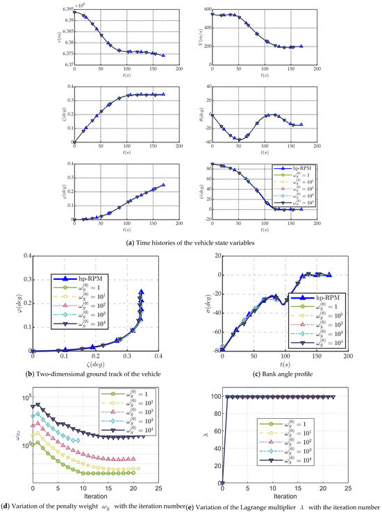
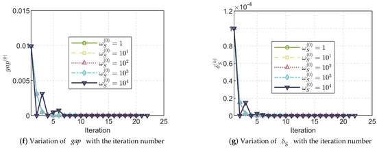
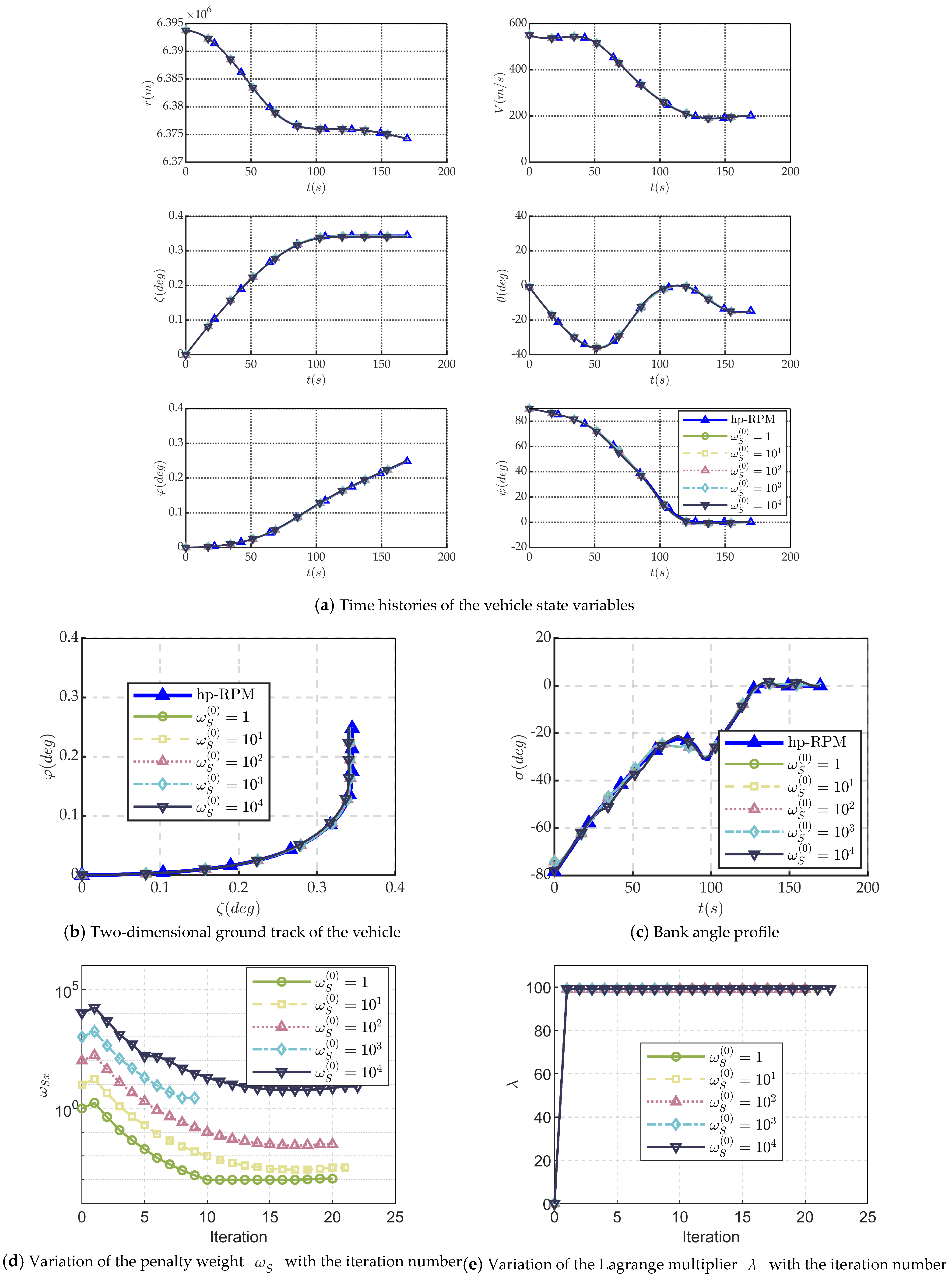
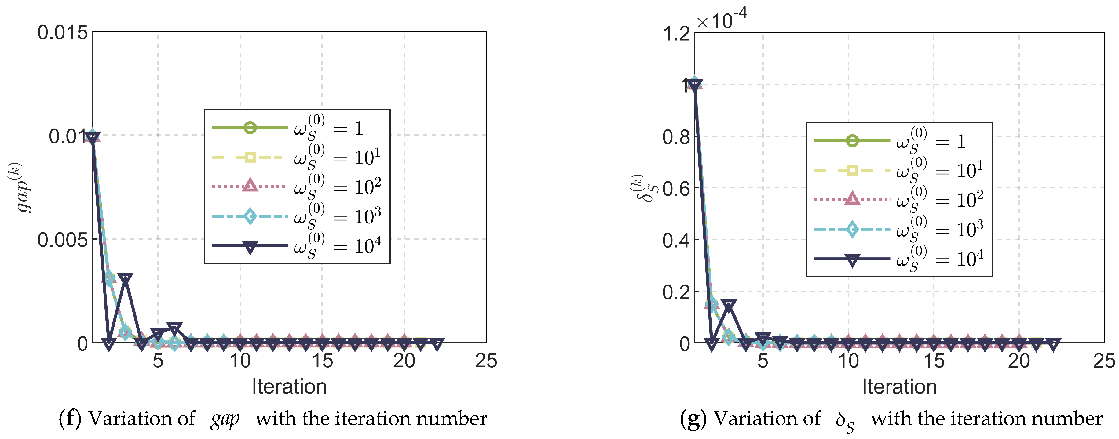
The corresponding results of the CGD-ASCP algorithm are presented in Figure 1, where the time histories of the vehicle state variables are shown in Figure 1a, the two-dimensional ground track is shown in Figure 1b, the bank angle profile is shown in Figure 1c, and the variations of the algorithm parameters ${\omega }_S,\lambda ,gap$, and ${\delta }_S$ with the iteration number are shown in Figure 1d–g. As can be observed from Figure 1a,b, within the currently set range of initial penalty weights, Algorithm 1 is able to converge stably to the vicinity of the optimal solution in all cases.

Figure 1. Simulation results with the parameters of Algorithm 1.

In the bank angle profile shown in Figure 1c, the control variable obtained by Algorithm 1 exhibits slight deviations from the optimal control; nevertheless, the state variable profiles still converge well to their optimal values, indicating that Algorithm 1 possesses favorable robustness against control deviations.

As shown in the variation curves of ${\omega }_S$ in Figure 1d, under all initial penalty weights, ${\omega }_S$ increases slightly after the first iteration and then smoothly converges to a reasonable steady-state value as the number of iterations increases, with no noticeable oscillations in the convergence process. The numbers of iterations when the initial value of ${\omega }_S$ is $1,{10}^1,{10}^2,{10}^3,{10}^4$ are 20, 21, 20, 9, and 22, respectively. When the initial penalty weight is ${10}^4$, ${\omega }_S$ converges stably from the initial value to 8.28, indicating that the proposed adaptive update law possesses favorable weight adjustment capability. The stable convergence of ${\omega }_S$ under all weights verifies the robustness of the CGD-ASCP algorithm with respect to the initial weight.

As shown in the $\lambda$ variation curve in Figure 1e, after the first iteration, $\lambda$ increases from its initial value of 0 to approximately 99.1 and subsequently remains stable around this value. From the $gap$ variation curve in Figure 1f, it can be observed that at the first iteration, $gap$ is on the order of $10^{-2}$, $\epsilon$ is on the order of ${10}^{-6}$, and ${\gamma }_{gap}$ is on the order of ${10}^{-2}$; consequently, the normalized complementarity gap term ${\gamma }_{gap}\cdot gap/(\lambda +\epsilon )$ is on the order of ${10}^2$, which drives $\lambda$ to jump to approximately 99.1. Thereafter, in combination with the variation curve of the equality constraint relaxation trust-region upper bound ${\delta }_S$ in Figure 1g, as the constraint violation is rapidly reduced to the order of ${10}^{-9}$ and the magnitude of $gap$ drops from ${10}^{-3}$ to ${10}^{-4}$ after the second iteration and stabilizes at ${10}^{-6}$ after the seventh iteration, both incremental terms in the $\lambda$ update formula tend to zero; hence, $\lambda$ no longer increases significantly. According to Lemma 2, $\left|\right|v|{|}_2$ is bounded. During the actual iterative process, $\left|\right|v|{|}_2$ gradually converges to about 26, while $\lambda$ is approximately 99.1, yielding $\eta =\left|\right|v|{|}_2/(\lambda +\epsilon )\approx 0.26$, which is on the same order of magnitude as the adaptive target final value ${\eta }_{\mathrm{target}}^{\mathrm{final}}=0.1$. The steady-state multiplier $\lambda$, through the penalty term in the objective function, ensures that the penalty intensity is sufficient to maintain constraint satisfaction while simultaneously preserving adequate adjustment margin for the adaptive update of ${\omega }_S$. Therefore, the stabilization of $\lambda$ signifies that the CGD-ASCP algorithm has converged to the vicinity of a KKT point of the original problem, which is consistent with the theoretical predictions of Lemma 4 and Lemma 5. Furthermore, the CGD-ASCP algorithm is able to compress the complementarity gap to ${10}^{-7}$ or below within only a few iterations, indicating that the algorithm can rapidly and stably satisfy the complementarity slackness condition and exhibits high convergence efficiency.

As shown in the ${\delta }_S$ variation curve in Figure 1g, at the first iteration, ${\delta }_S$ is on the order of ${10}^{-4}$; at this stage, the dynamic upper bound provides the subproblem with a reasonable initial relaxation space, thereby guaranteeing the feasibility of the subproblem. After the second iteration, the magnitude of ${\delta }_S$ drops to ${10}^{-5}$–${10}^{-6}$ and is subsequently further compressed and stabilized at the order of ${10}^{-9}$ to ${10}^{-10}$. Therefore, the dynamic ${\delta }_S$ upper bound mechanism of the CGD-ASCP algorithm is able to offer sufficient feasibility space in the early stage and subsequently tighten the relaxation radius through adaptive updates, ensuring that the final solution satisfies the original equality constraints. Although the initial penalty weights span a wide range of orders of magnitude, both $gap$ in Figure 1f and ${\delta }_S$ in Figure 1g exhibit favorable convergence behavior, satisfying the convergence accuracy requirements within only 6–7 steps, which reflects the robustness of the CGD-ASCP algorithm with respect to the initial penalty weight. The iteration data of the CGD-ASCP algorithm are listed in Table 3.

Table 3. Iteration time and iteration accuracy of the CGD-ASCP algorithm.

Initial Weight	$1$	$10^1$	$10^2$	$10^3$	$10^4$
Average time per iteration (s)	0.024	0.024	0.025	0.025	0.026
Number of iterations	20	21	20	9	22
Total time (s)	0.480	0.504	0.500	0.225	0.572
Terminal error (km)	0.420	0.418	0.415	0.418	0.420

It can be observed from Table 3 that the time per iteration of the CGD-ASCP algorithm is on the order of 30 ms, and the total solution time is on the order of 0.5 s, while the total solution time of hp-RPM is 0.945 s. By comparison, the total solution time of the CGD-ASCP algorithm is reduced by approximately 51.7% on average. When ${\omega }_S^{(0)}={10}^3$, the CGD-ASCP algorithm requires the fewest iteration steps, with a solution time of 0.225 s, corresponding to a 76.2% reduction in total solution time, making its advantage in solution time even more prominent. In addition, the position error of the CGD-ASCP algorithm relative to the optimal solution stabilizes within 0.5 km, and its solution quality is insensitive to the initial weight. Therefore, the complementarity-gap-driven adaptive update strategy adopted by the CGD-ASCP algorithm exhibits favorable robustness with respect to the initial penalty weight as well as good convergence accuracy, and possesses potential for applications in scenarios with high real-time requirements, such as online trajectory planning.

5. Conclusions

To address the issue that the penalty weight update strategy in the augmented Lagrangian multiplier method is sensitive to initial weights, this paper proposes a complementarity-gap-driven adaptive sequential convex programming algorithm. By introducing the complementarity slackness condition into the parameter update law, the algorithm employs the complementarity slackness ratio and the complementarity gap as feedback signals to drive the adaptive adjustment of the penalty weight and the Lagrange multiplier, respectively. This enables the algorithm to automatically modulate the penalty intensity according to the current degree of constraint violation, thereby achieving closed-loop cooperative control. The main conclusions of this paper can be summarized as follows:

(1) A complementarity-gap-driven adaptive sequential convex programming algorithm is proposed. By using the complementarity slackness ratio and the complementarity gap to drive the adaptive updates of the penalty weight and the Lagrange multiplier, respectively, closed-loop cooperative control is realized and the robustness with respect to the initial penalty weight is enhanced.

(2) A complete theoretical convergence analysis framework for the CGD-ASCP algorithm is established. The monotonic bounded convergence of the Lagrange multiplier and the convergence of the slack variables and the complementarity gap are rigorously proved, and a conditional convergence theorem is presented.

(3) Numerical simulations on the reentry trajectory planning problem of a gliding vehicle show that, when the initial penalty weight spans five orders of magnitude from 1 to ${10}^4$, the average solution time of the CGD-ASCP algorithm is 0.46 s, which is shortened by approximately 51.7% compared with the total solution time of hp-RPM. Moreover, the algorithm exhibits favorable stable convergence and terminal accuracy under all initial weights, demonstrating good computational efficiency and weight robustness.

(4) Future work will focus on the exploratory application of the proposed adaptive strategy in complex scenarios such as online no-fly zone avoidance, so as to serve the guidance and control requirements of cross-domain vehicles.

References

- Rao, A.V. A Survey of Numerical Methods for Optimal Control. In Proceedings of the AAS/AIAA Astrodynamics Specialist Conference, Pittsburgh, PA, USA, 9–13 August 2009. [Google Scholar]
- Malyuta, D.; Yu, Y.; Elango, P.; Acikmese, B. Advances in Trajectory Optimization for Space Vehicle Control. Annu. Rev. Control 2021, 52, 282–315. [Google Scholar] [CrossRef] [Scilit]
- Betts, J.T. Survey of Numerical Methods for Trajectory Optimization. J. Guid. Control Dyn. 1998, 21, 193–207. [Google Scholar] [CrossRef] [Scilit] [PubMed]
- Wang, Z. A Survey on Convex Optimization for Guidance and Control of Vehicular Systems. Annu. Rev. Control. 2024, 57, 100957. [Google Scholar] [CrossRef] [Scilit]
- Boyd, S.; Vandenberghe, L. Convex Optimization; Cambridge University Press: Cambridge, UK, 2004; pp. 1–22. [Google Scholar]
- Acikmese, B.; Ploen, S.R. Convex Programming Approach to Powered Descent Guidance for Mars Landing. J. Guid. Control Dyn. 2007, 30, 1353–1366. [Google Scholar] [CrossRef] [Scilit]
- Blackmore, L.; Acikmese, B.; Scharf, D.P. Minimum-Landing-Error Powered-Descent Guidance for Mars Landing Using Convex Optimization. J. Guid. Control Dyn. 2010, 33, 1161–1171. [Google Scholar] [CrossRef] [Scilit]
- Luo, D.; Spada, F.; Acikmese, B. Discrete-Time Lossless Convexification for Pointing Constraints. IEEE Control Syst. Lett. 2025, 9, 246–251. [Google Scholar] [CrossRef] [Scilit]
- Schulman, J.; Duan, Y.; Ho, J.; Lee, A.; Awwal, I.; Bradlow, H.; Pan, J.; Patil, S.; Goldberg, K.; Abbeel, P. Motion Planning with Sequential Convex Optimization and Convex Collision Checking. Int. J. Robot. Res. 2014, 33, 1251–1270. [Google Scholar] [CrossRef] [Scilit]
- Lu, P.; Liu, X. Autonomous Trajectory Planning for Rendezvous and Proximity Operations by Conic Optimization. J. Guid. Control Dyn. 2013, 36, 375–389. [Google Scholar] [CrossRef] [Scilit]
- Liu, X.; Lu, P. Solving Nonconvex Optimal Control Problems by Convex Optimization. J. Guid. Control Dyn. 2014, 37, 750–765. [Google Scholar] [CrossRef] [Scilit]
- Wang, Z.; Grant, M.J. Minimum-Fuel Low-Thrust Transfers for Spacecraft: A Convex Approach. IEEE Trans. Aerosp. Electron. Syst. 2018, 54, 2274–2290. [Google Scholar] [CrossRef] [Scilit]
- Wang, Z.; Grant, M.J. Optimization of Minimum-Time Low-Thrust Transfers Using Convex Programming. J. Spacecr. Rockets 2018, 55, 586–598. [Google Scholar] [CrossRef] [Scilit]
- Sagliano, M.; Mooij, E. Optimal Drag-Energy Entry Guidance via Pseudospectral Convex Optimization. Aerosp. Sci. Technol. 2021, 117, 106946. [Google Scholar] [CrossRef] [Scilit]
- Bonalli, R.; Cauligi, A.; Bylard, A.; Pavone, M. GuSTO: Guaranteed Sequential Trajectory Optimization via Sequential Convex Programming. In Proceedings of the 2019 International Conference on Robotics and Automation (ICRA), Montreal, QC, Canada, 20–24 May 2019. [Google Scholar]
- Malyuta, D.; Reynolds, T.P.; Szmuk, M.; Lew, T.; Bonalli, R.; Pavone, M.; Acikmese, B. Convex Optimization for Trajectory Generation: A Tutorial on Generating Dynamically Feasible Trajectories Reliably and Efficiently. IEEE Control Syst. Mag. 2022, 42, 40–113. [Google Scholar] [CrossRef] [Scilit]
- Mao, Y.Q.; Szmuk, M.; Acikmese, B. Successive Convexification of Non-Convex Optimal Control Problems and Its Convergence Properties. In Proceedings of the 2016 IEEE 55th Conference on Decision and Control (CDC), Las Vegas, NV, USA, 12–14 December 2016. [Google Scholar]
- Mao, Y.Q.; Dueri, D.; Szmuk, M.; Acikmese, B. Successive Convexification of Non-Convex Optimal Control Problems with State Constraints. IFAC-PapersOnLine 2017, 50, 4063–4069. [Google Scholar] [CrossRef] [Scilit]
- Szmuk, M.; Acikmese, B. Successive Convexification for 6-DoF Mars Rocket Powered Landing with Free-Final-Time. In Proceedings of the 2018 AIAA Guidance, Navigation, and Control Conference, Kissimmee, FL, USA, 8–12 January 2018. [Google Scholar]
- Roh, H.; Oh, Y.J.; Tahk, M.J.; Kwon, K.J.; Kwon, H.H. L1 Penalized Sequential Convex Programming for Fast Trajectory Optimization: With Application to Optimal Missile Guidance. Int. J. Aeronaut. Space Sci. 2020, 21, 493–503. [Google Scholar] [CrossRef] [Scilit]
- Benedikter, B.; Zavoli, A.; Colasurdo, G.; Pizzurro, S.; Cavallini, E. Convex Approach to Three-Dimensional Launch Vehicle Ascent Trajectory Optimization. J. Guid. Control Dyn. 2021, 44, 1116–1131. [Google Scholar] [CrossRef] [Scilit]
- Li, Y.; Chen, W.C.; Yang, L. Successive Chebyshev Pseudospectral Convex Optimization Method for Nonlinear Optimal Control Problems. Int. J. Robust Nonlinear Control 2022, 32, 326–343. [Google Scholar] [CrossRef] [Scilit]
- Dong, C.L.; Xie, L.; He, R.Z.; Zhou, X.; Zhang, H.B. Weight-Adaptive Augmented Lagrange Multiplier Sequential Convex Programming for Nonlinear Trajectory Optimization. Aerosp. Sci. Technol. 2024, 155, 109527. [Google Scholar] [CrossRef] [Scilit]
- Xie, L.; He, R.Z.; Zhang, H.B.; Tang, G.J. Oscillation Phenomenon in Trust-Region-Based Sequential Convex Programming for the Nonlinear Trajectory Planning Problem. IEEE Trans. Aerosp. Electron. Syst. 2022, 58, 3337–3352. [Google Scholar] [CrossRef] [Scilit]
- Szmuk, M.; Reynolds, T.P.; Acikmese, B. Successive Convexification for Real-Time Six-Degree-of-Freedom Powered Descent Guidance with State-Triggered Constraints. J. Guid. Control Dyn. 2020, 43, 1399–1413. [Google Scholar] [CrossRef] [Scilit]
- Sherali, H.D.; Ozdaryal, B.; Adams, W.P.; Attia, N. On Using Exterior Penalty Approaches for Solving Linear Programming Problems. Comput. Oper. Res. 2001, 28, 1049–1074. [Google Scholar] [CrossRef] [Scilit]
- Yamashita, H.; Tanabe, T. A Primal-Dual Exterior Point Method for Nonlinear Optimization. SIAM J. Optim. 2010, 20, 3335–3363. [Google Scholar] [CrossRef] [Scilit][Green Version]
- Galvan, G.; Lapucci, M.; Levato, T.; Sciandrone, M. An Alternating Augmented Lagrangian Method for Constrained Nonconvex Optimization. Optim. Methods Softw. 2020, 35, 502–520. [Google Scholar] [CrossRef] [Scilit]
- Bonnans, J.F.; Shapiro, A. Perturbation Analysis of Optimization Problems; Springer: New York, NY, USA, 2000; pp. 290–299. [Google Scholar]
- Xie, Y.; Liu, L.H.; Liu, J.; Tang, G.J.; Zheng, W. Rapid Generation of Entry Trajectories with Waypoint and No-Fly Zone Constraints. Acta Astronaut. 2012, 77, 167–181. [Google Scholar] [CrossRef] [Scilit]
- Domahidi, A.; Chu, E.; Boyd, S. ECOS: An SOCP Solver for Embedded Systems. In Proceedings of the European Control Conference (ECC), Zurich, Switzerland, 17–19 July 2013. [Google Scholar]
Disclaimer/Publisher’s Note: The statements, opinions and data contained in all publications are solely those of the individual author(s) and contributor(s) and not of MDPI and/or the editor(s). MDPI and/or the editor(s) disclaim responsibility for any injury to people or property resulting from any ideas, methods, instructions or products referred to in the content. |
© 2026 by the authors. Licensee MDPI, Basel, Switzerland. This article is an open access article distributed under the terms and conditions of the Creative Commons Attribution (CC BY) license.