A Grid-Based Optimization Method for Airspace Conflict Detection and Resolution During the Execution Phase

Abstract

Growing air traffic and dynamic missions require conflict detection and resolution (CD&R) during the execution phase, when ad hoc airspace must be inserted into an already conflict-free baseline plan without global re-optimization. This paper proposes a grid-based online optimization framework built on Geographical Coordinate Subdivision grid with One dimension integer coding on 2ⁿ-tree (GeoSOT) discretization that transforms four-dimensional spatiotemporal conflict judgment into efficient grid-code matching and interval comparison. Incremental conflict detection restricts pairwise checks to candidate ad hoc-related pairs, reducing detection scale by over 99% relative to full screening. A lexicographic two-stage resolution policy prioritizes ad hoc adjustments—incorporating horizontal, altitude, temporal, and grid-shrinkage operations—and activates limited baseline coordination only when necessary. The The Incremental Ad-hoc Operation—Tiered Priority Time-Sliced Search (IAO-TPTS) algorithm implements this policy under a hard time budget through Phase A (ad-hoc-restricted Dimension-wise Conflict-Driven Assignment, DCDA-Lite) for fast ad hoc-only feasibilization and Phase B (Hybrid Adaptive Large Neighborhood Search, Hybrid-ALNS) for tiered refinement, with dual validation to prevent secondary conflicts in neighboring airspace. Experiments including visualization, ablation, algorithm comparison, and scalability analysis on Small, Medium, and Large scenarios show 100% feasibility within 180 s, median solve times as low as 0.069 s, competitive objective values versus mixed-integer linear programming (MILP) and Adaptive Large Neighborhood Search (ALNS), and sub-linear scalability from 20 to 300 baseline airspaces. The novelty is this integrated execution-phase framework (incremental detection, lexicographic baseline-protective scheduling, and time-budgeted IAO-TPTS with dual validation), rather than a new grid-coding scheme or a standalone MILP.

1. Introduction

With the rapid growth of global air traffic and the emergence of new aviation concepts such as Unmanned Aerial Vehicles (UAVs) and urban air mobility, the density, dynamism, and complexity of airspace systems have reached an unprecedented level [1]. Conflict detection and resolution (CD&R) serves as a core technical safeguard to maintain flight separation and prevent collisions, remaining a prominent research focus in Air Traffic Management (ATM) [1]. The promotion of 4-D trajectory concepts has provided a foundation for the precise representation of flight intentions, but it also renders the CD&R problem more intricate: it requires maintaining safe spatial separations while also ensuring pre-scheduled temporal compliance, especially when ad hoc missions arise online [2]. How to respond rapidly while preserving baseline plans constitutes the core challenge of conflict resolution during the execution phase.

The research problem is therefore execution-phase CD&R under ad hoc airspace insertion: a certified, conflict-free baseline is already in force, new occupancies arrive online, and occupancy exclusivity must be restored within a hard wall-clock budget without globally replanning the baseline. This problem is significant because an execution-phase conflict is an operational event rather than a pre-tactical design residual: an unresolved occupancy overlap, or a cascade of baseline revisions, degrades both safety and schedule integrity. In practice, the setting matches temporary missions, emergency support, and dynamic UAV/UAM demands that must be inserted into an already cleared plan; the usable output is a dual-validated occupancy adjustment that prefers changing only the new demand and, if unavoidable, only a local baseline subset.

Traditional CD&R research has predominantly focused on strategic or pre-tactical phases. For instance, large-scale 4D trajectory strategic de-confliction methods model conflict optimization as network-constrained problems, yet pre-planning is largely completed before execution [3,4]. Meanwhile, tactical conflict detection in terminal airspace emphasizes strict requirements for low false-alarm rates and high response speeds [3]. Other approaches, such as weighted-graph methods for dynamic airspace management [5] and distributed separation assurance algorithms under high-density autonomous flight scenarios [6], attempt to address real-time dynamics in an online, scalable manner. However, these methods often fail to explicitly distinguish the priorities between “newly inserted/ad-hoc demands” and “already established baseline plans that should be protected.”To achieve efficient spatiotemporal indexing and rapid conflict judgment during online resolution, discretizing continuous airspace and time into grids has emerged as a highly promising technique. The global subdivision grid model, the global subdivision grid model, Geographical Coordinate Subdivision grid with One dimension integer coding on 2ⁿ-tree (GeoSOT), provides a unified integer coding system for any region in Earth’s space through multi-scale and hierarchical subdivision [7]. Based on the 4D spatiotemporal grid model (GeoSOT-AS), data extraction performance can be significantly enhanced [8,9]. Parallel to data management, researchers have focused on using grid methods to accelerate conflict computation itself. For instance, Acevedo et al. utilized 4D grids to transform traditional quadratic complexity checking into linear complexity by only checking neighboring grid units [10]. Similarly, Miao et al. proposed a low-altitude flight conflict detection algorithm based on GeoSOT, substituting traditional traversal with spatial indexing and database partitioning to achieve exponential efficiency gains [11]. Furthermore, Zhai et al. extended this concept to construct low-altitude public air route networks using global subdivision grids [12]. An et al. further showed that grid-partitioned airspace can represent restricted areas and support route planning with obstacle avoidance [13]. While these studies demonstrate that grid mapping transforms conflict detection into spatial grid-occupation queries—effectively converting trajectory adjustment into discrete search problems suitable for fast online calculation—existing grid-based studies remain largely focused on data management or strategic conflict detection. They have not yet been systematically introduced into conflict resolution and optimization during the execution phase. Specifically, under the constraint of “protecting the existing baseline plan while prioritizing the adjustment of newly inserted objects,” designing efficient meta-heuristics and matching grid layers with resolution priorities remains an open challenge [11,12].

In recent years, scholars have explored various alternative methods to address CD&R. Mathematical programming methods, such as mixed-integer linear programming (MILP), can return a global optimum when the solver closes the optimality gap, but they become a computational bottleneck in large-scale or wall-clock-capped settings [14,15]. Geometric methods (e.g., Velocity Obstacles) and traditional meta-heuristics like Particle Swarm Optimization (PSO) and standard Differential Evolution (DE) offer fast computation but often encounter premature convergence and stagnation in continuous resolution tasks [16,17]. Furthermore, general multi-UAV conflict resolution approaches often lack localized coordination mechanisms, leading to high computational overhead [18]. To build upon advanced optimization techniques, Adaptive Large Neighborhood Search (ALNS) and its operator mechanisms provide robust theoretical foundations for neighborhood-based meta-heuristics [19]. Moreover, recent spatially and temporally integrated strategies highlight the importance of balancing local airspace capacities through vertical and temporal changes, though gaps remain in handling ad hoc execution-phase insertions without system-wide disruptions [20]. Spatial correlation has also been examined in related aviation-system studies. Urban economic structure has been linked to passenger and freight efficiencies across Chinese airports using a two-stage method [21], and dynamic–static multi-graph spatial–temporal networks have been used to predict flight delays [22]. These works capture spatial or network dependence in airport operations and delay propagation, but they do not address execution-phase airspace-occupancy CD&R or baseline-protective ad hoc insertion.

Grid studies [7,8,9,10,11,12,13] mainly improve representation, indexing, and detection. Optimization studies [14,15,16,17,18,19,20] provide MILP, PSO, DE, or ALNS-style search, but they typically adjust all involved objects and do not encode a lexicographic duty to leave a certified baseline unchanged under a tight online budget. The novelty of this paper is therefore neither a new GeoSOT coding system nor a new standalone solver. It is an integrated execution-phase CD&R framework whose distinctive element is the online scheduling policy: incremental P_adhoc detection, Stage-1/Stage-2 lexicographic baseline protection, and Incremental Ad-hoc Operation—Tiered Priority Time-Sliced Search (IAO-TPTS) (ad-hoc-restricted Dimension-wise Conflict-Driven Assignment, DCDA-Lite then Hybrid Adaptive Large Neighborhood Search, Hybrid-ALNS) with dual validation under a wall-clock limit. Table 1 compares the present work with representative studies along the dimensions of operation phase, spatial representation, temporal representation, conflict definition, adjustable objects, baseline-plan protection, optimization method, and validation mechanism.

Table 1. Comparison with representative grid-based studies.

Study	Operation Phase	Spatial Representation	Temporal Representation	Conflict Definition	Adjustable Objects	Baseline-Plan Protection	Optimization Method	Validation Mechanism
GeoSOT/GeoSOT-AS/BeiDou grid [7,8,9]	Modeling/data management	GeoSOT or BeiDou cells	4D attributes [8] or none	Occupancy/index, not insertion CD&R	—	—	Grid coding	Data/mapping tests
Acevedo et al. [10]	Tactical multi-UAV detection	4D grid	Time-stamped cells	Neighbor-cell check	Trajectories (detection)	No	Spatial index	Detection complexity
Miao et al. [11]	Low-altitude detection	Multi-level GeoSOT	Spatiotemporal index	Grid-index overlap	—	No	DB partition/index	Detection efficiency
Zhai et al. [12]	Strategic route network	Global subdivision grid	Route occupancy	Network construction	Route layout	No	Grid network design	Network case
An et al. [13]	Pre-flight route planning	Uniform grid	Static	Restricted-cell avoidance	Path	No	Cell path search	Planning examples
MILP/IP [14,15]	Strategic/pre-tactical	Continuous or hex grid [15]	Time windows/discretisation	Geometric/cell conflict	Typically all aircraft	No ad hoc vs. baseline split	MILP/IP	Optimality on limited size
PSO/DE [16,17]	Tactical trajectory CD&R	Continuous 3D	Trajectory time	Distance/loss of separation	Involved flights	No	PSO/DE	Simulation
Multi-UAV CR [18]	Online multi-agent	Mixed	Trajectory	Pairwise conflict	Multiple UAVs	No local baseline lock	Heuristic CR	Simulation
ALNS operators (Voigt) [19]	VRP (not CD&R)	—	—	—	—	—	ALNS destroy/repair	VRP benchmarks
Yang et al. [20]	Medium-term urban airspace	Spatially integrated	Temporally integrated	Medium-term CD&R	Capacity/flow	Not execution-phase insertion	Spatiotemporal strategy	Urban scenarios
This work	Execution-phase ad hoc insertion	GeoSOT codes G	Closed interval T	Occupancy overlap of G, H, T (Equations (15)–(18))	Ad hoc first; local T2 only if Stage 1 uncertified	Lexicographic z0; T2 locked if Stage 1 certified	IAO-TPTS: DCDA-Lite + Hybrid-ALNS	Dual validation on complete V_stage

These shortcomings map onto the work of this paper as follows. Because grid studies [7,8,9,10,11,12,13] mainly stop at representation, indexing, or detection, online checks are restricted to the incremental pair set involving newly inserted occupancies. Because optimization studies [14,15,16,17,18,19,20] typically adjust all involved objects and do not encode a duty to leave a certified baseline unchanged, a lexicographic Stage-1/Stage-2 policy is imposed: Stage 2 unlocks a conflict-related baseline subset only when Stage-1 feasibility is not certified. Because a time-capped solver cannot be treated as a proven global optimum, IAO-TPTS schedules existing search components under a wall-clock limit and dual-validates every accepted occupancy. Table 1 summarizes this gap-to-contribution relation.

To bridge these gaps, this paper proposes a grid-based online optimization and scheduling method for execution-phase CD&R. As summarized in Table 1, the contribution is an integrated framework rather than a new grid code or a new standalone solver. The main contributions are as follows:

Incremental grid-based conflict detection: Online checks are restricted to candidate pairs involving newly inserted occupancies on the existing GeoSOT base map, so a global rescan of the certified baseline is avoided.

Lexicographic two-stage online Strategy: Stage 1 adjusts newly inserted objects only. Stage 2 unlocks a conflict-related baseline subset only when Stage-1 feasibility is not certified; if Stage 1 is certified, baseline (T2) objects remain locked. This is the baseline-protection rule, not a cost-weight heuristic alone.

Time-budgeted integration of existing search components: IAO-TPTS schedules DCDA-Lite (Phase A) and Hybrid-ALNS (Phase B) on localized grid primitives under a hard wall-clock limit, with dual validation on the complete stage-wise pair set. The search operators are adapted from existing methods; the novelty is the scheduling, the adjustable-set policy, and the validation gate, not a new meta-heuristic from scratch.

2. Four-Dimensional Spatiotemporal Discretization for Ad Hoc Airspace Insertion Based on a Two-Dimensional Grid

During the pre-planning stage, the original airspace demands have been gridded, checked for conflicts, and resolved into a baseline conflict-free airspace plan satisfying four-dimensional spatiotemporal separation [2]. Since the airspace objects in this baseline plan are already mutually conflict-free, global conflict detection and resolution among all existing objects need not be repeated during the ad hoc implementation phase.

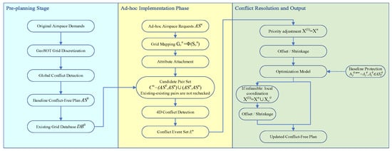
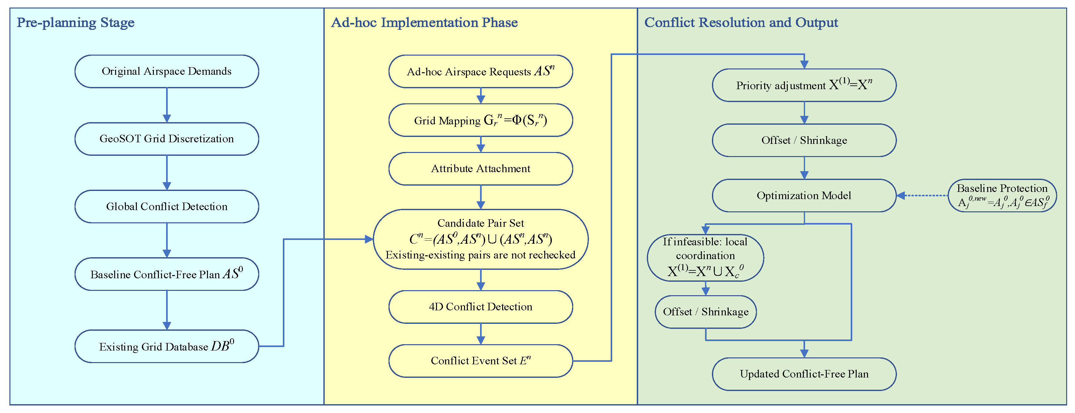
During actual operation, however, ad hoc missions, temporary control requirements, emergency support tasks, or dynamically generated demands may appear. These newly inserted airspace objects must be incorporated into the current plan without compromising the safety of the existing baseline [1]. The core task of the ad hoc implementation phase is therefore to detect and resolve only the conflicts related to newly inserted airspace objects through incremental adjustment. The overall research framework is shown in Figure 1, which lists the inputs, the processing modules, and the outputs.

Figure 1. Overall framework of the grid-based online optimization method for ad hoc airspace insertion during the execution phase (inputs, process, and outputs).

Figure 1 summarizes the research mechanism. Inputs: a certified, conflict-free baseline stored as GeoSOT occupancies, and one or more ad hoc requests that are not yet on that map, together with the online adjustment bounds (detailed in Section 3) and the wall-clock budget. Process: each request is mapped to a grid occupancy (G, H, T); conflicts are tested only on pairs that involve at least one ad hoc object; if any occupancy conflict remains, IAO-TPTS searches under the lexicographic Stage-1/Stage-2 rule with dual validation. Outputs: the updated occupancies, a feasibility certificate, the objective J, the runtime, and whether any baseline object was modified (z⁰). Newly inserted airspace objects are adjusted with priority. If conflicts can be resolved by adjusting them alone, all existing objects remain unchanged; otherwise, only the conflict-related local subset of existing objects is allowed limited coordination, while objects outside this subset remain fixed, and no global re-optimization of the baseline plan is performed.

Let the set of existing airspace objects resolved during the pre-planning stage be

$$A{S}^0=\{A_1^0,A_2^0,\dots ,A_m^0\}$$

(1)

and the set of newly inserted ad hoc airspace objects be

$$A{S}^n=\{A_1^n,A_2^n,\dots ,A_q^n\}$$

(2)

where the superscript 0 denotes existing airspace, and the superscript n denotes newly inserted airspace.

Since conflicts among existing objects have already been resolved in the pre-planning stage, this phase focuses on two conflict types only: (i) conflicts between newly inserted and existing objects, and (ii) conflicts among newly inserted objects themselves. Conflicts among existing objects are not re-checked, except that, when a small number of existing objects participate in local coordination, only their conflicts with immediate neighbors are verified—not a global re-detection.

2.1. Existing Airspace Grid Database and Unified Base Map

During the pre-planning stage, all existing airspace objects have been discretized based on a unified GeoSOT two-dimensional grid system. Each existing object is represented as

$$A_i^0=(G_i^0,H_i^0,T_i^0,p_i^0)$$

(3)

Denotes the GeoSOT grid-code set occupied by the existing airspace object $A_i^0$, $H_i^0$ denotes its occupied altitude interval, $T_i^0$ denotes its time window; and $p_i^0$ denotes its mission priority or adjustment sensitivity. Each tuple $(G,H,T,p)$ denotes a protected airspace occupancy, not the raw mission geometry of an aircraft. The occupancy is specified first in continuous space. Horizontal separation, vertical separation, and the temporal buffer are embedded when this occupancy is generated, and are then inherited by G, H, and T. Subsequent GeoSOT mapping records the occupancy; it does not add a second online separation layer.

Because the baseline plan is already conflict-free,

$$I_{ij}^0=0,\forall A_i^0,A_j^0\in A{S}^0,i\ne j$$

(4)

The altitude interval and time window can be written as

$$H_i^0=[h_{i,\min }^0,h_{i,\max }^0]$$

(5)

$$T_i^0=[t_{i,\min }^0,t_{i,\max }^0]$$

(6)

The existing airspace objects have already satisfied the conflict-free condition. That is, for any two different existing airspace objects $A_i^0$ and $A_j^0$

$$I\left(A_i^0,A_j^0\right)=0,\forall i\ne j$$

(7)

where $I_{ij}^0$ denotes the conflict indicator between $A_i^0$ and $A_j^0$; $I_{ij}^0=0$ means no four-dimensional spatiotemporal conflict.

The existing airspace grid database is

$$D{B}^0=\{R_i^0(g)\mid A_i^0\in A{S}^0,g\in G_i^0\}$$

(8)

with each record given by

$$R_i^0(g)=(g,H_i^0,T_i^0,p_i^0)$$

(9)

This database stores the horizontal grid occupation, altitude interval, time window, and priority information of existing airspace objects, providing a unified data basis for the rapid insertion and conflict detection of newly inserted ad hoc airspace objects [8].

2.2. Grid Mapping and Attribute Attachment of Newly Inserted Ad Hoc Airspace

Newly inserted ad hoc airspace objects may take various forms, such as circular areas, polygonal areas, route corridors, mission protection zones, or temporary restricted areas [12]. To enable conflict detection between newly inserted and existing airspace objects within the same data structure, newly inserted objects are represented using the same GeoSOT grid-coding system as that used in the pre-planning stage [9].

For a newly inserted airspace object $A_r^n$, its specified protected occupancy is

$$A_r^n=(S_r^n,H_r^n,T_r^n,p_r^n)$$

(10)

where $S_r^n$ denotes its drawn horizontal region, $H_r^n$, $T_r^n$ its requested altitude interval and time window, and $p_r^n$ its priority.

The horizontal footprint is first mapped into grid cells:

$$G_r^n=\mathsf{\Phi }(S_r^n)=\{g\mid \mathrm{g}\cap S_r^n\ne \varnothing \}$$

(11)

The protected airspace is drawn first in continuous space and is then mapped onto the unified GeoSOT base map. A cell is included in $G_r^n$ whenever it intersects $S_r^n$. This intersection rule is a conservative outer-envelope covering (staircasing). It is a discretization effect, not an additional operational buffer applied at detection time.

After horizontal grid mapping, the altitude interval and time window are attached to the occupied grid codes as attributes:

$$R_r^n(g)=(g,H_r^n,T_r^n,p_r^n),g\in G_r^n$$

(12)

The newly inserted airspace grid database is then

$$D{B}^n=\{R_r^n(g)\left|g\in G_r^n,\right.A_r^n\in A{S}^n\}$$

(13)

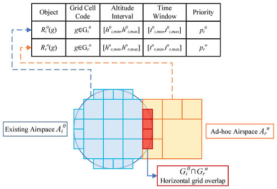
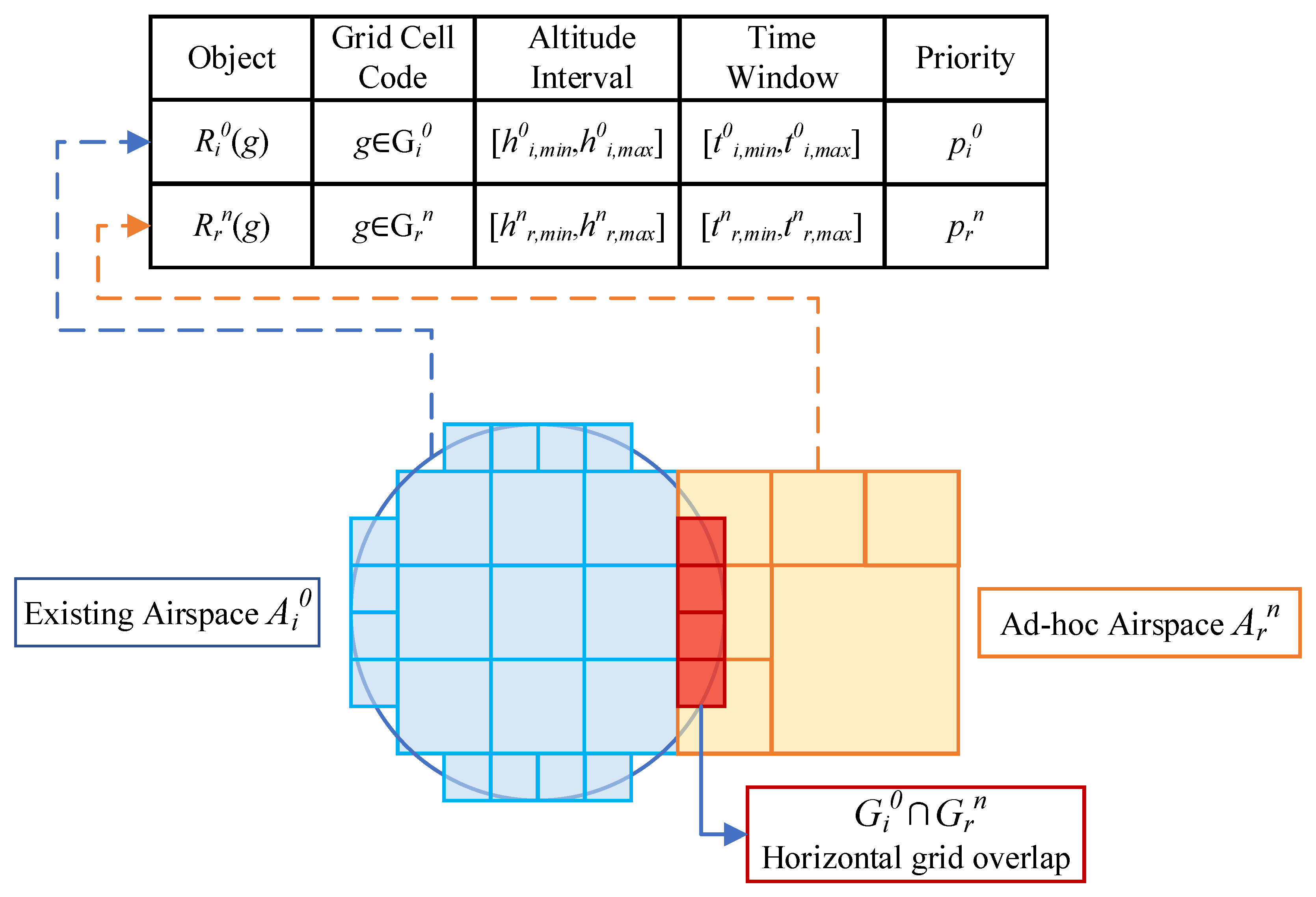
Figure 2 illustrates the unified grid-attribute representation of existing and newly inserted airspace objects, as well as the horizontal grid overlap between them.

Figure 2. Unified grid-attribute representation and horizontal grid overlap between existing and newly inserted airspace objects. Dashed arrows indicate the correspondence between each airspace object and its grid-attribute record; red overlapping cells indicate horizontal grid overlap.

It should be noted that although altitude and time appear in the same grid-attribute record, they jointly describe independent physical dimensions of the airspace object. In the subsequent conflict-judgment process, altitude overlap and time overlap are always evaluated independently and are never combined into a single mixed condition [20].

2.3. Conflict Detection Model for Ad Hoc Airspace Insertion

During the ad hoc implementation phase, full pairwise conflict detection among all airspace objects is unnecessary. Only candidate pairs related to newly inserted objects need to be checked:

$$C^n=\left(A{S}^0,A{S}^n\right)\cup \left(A{S}^n,A{S}^n\right)$$

(14)

For each candidate pair $(A_u,A_v)\in C^n$, the horizontal overlap indicator is defined as

$$I_{uv}^G=\left\{\begin{array}{c}1,G_u\cap G_v\ne \varnothing \hfill \\ 0,otherwise\hfill \end{array}\right.$$

(15)

the altitude overlap indicator as

$$I_{uv}^H=\left\{\begin{array}{c}1,max(h_{u,min},h_{v,min})\le min(h_{u,max},h_{v,max})\hfill \\ 0,otherwise\hfill \end{array}\right.$$

(16)

and the time overlap indicator as

$$I_{uv}^T=\left\{\begin{array}{c}1,max(t_{u,min},t_{v,min})\le min(t_{u,max},t_{v,max})\hfill \\ 0,otherwise\hfill \end{array}\right.$$

(17)

The four-dimensional conflict indicator is defined as their product:

$$I_{uv}=I_{uv}^G\cdot I_{uv}^H\cdot I_{uv}^T$$

(18)

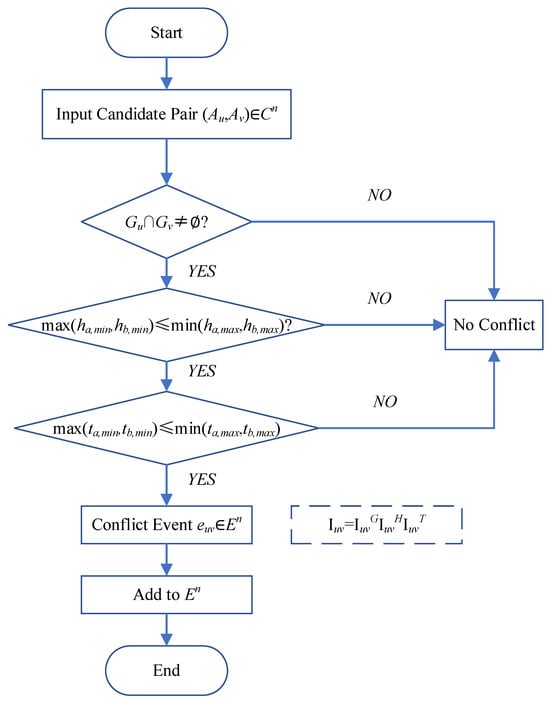
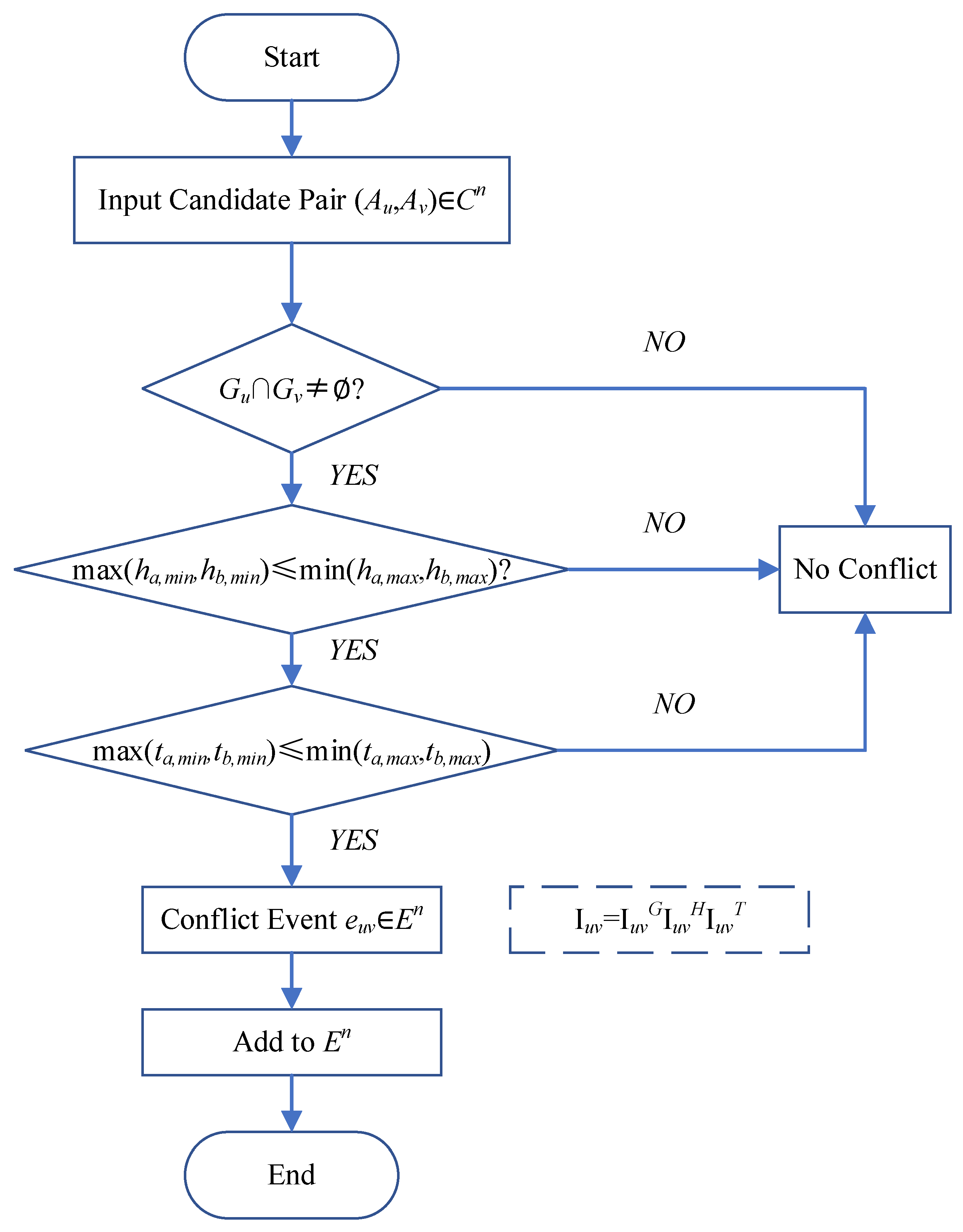
$I_{uv}=1$ indicates that the two objects overlap simultaneously in the horizontal, altitude, and time dimensions, i.e., an occupancy conflict of protected airspace, not an aircraft-level loss of separation; separation in any single dimension yields $I_{uv}=0$. The sequential judgment process is shown in Figure 3.

Figure 3. Flowchart of four-dimensional conflict detection for a candidate airspace pair. Overlap of protected occupancies in all three dimensions is an occupancy conflict; boundary contact is treated as overlap.

Equations (15)–(18) declare a conflict when two objects overlap simultaneously in $G$, $H$, and $T$. This is an airspace-occupancy conflict: two protected occupancies are no longer exclusive. It is not a test of aircraft-level loss of separation. Because horizontal, vertical, and temporal protection are already embedded in the specified occupancies, the online detector does not impose extra buffers $d_h,\Delta h$, or $d_t\Delta t$ on top of $(G,H,T)$.

Horizontal coordinates are geodetic longitude and latitude in WGS84, encoded by GeoSOT codes on the unified base map (L_max = 14 in the experiments). Altitude is referenced to mean sea level (MSL); experimental objects occupy bands within 1000–8000 m MSL. Time windows are clock intervals on the operational day.

Interval endpoints are closed. Equations (16) and (17) use “≤”, so two altitude or time intervals that only touch at a boundary are judged to overlap; sharing a GeoSOT cell is likewise a horizontal overlap. This convention is intentional: the objects are already protected occupancies, so boundary contact means that the encoded safety margin has been used up. The test is conservative relative to an open-interval reading.

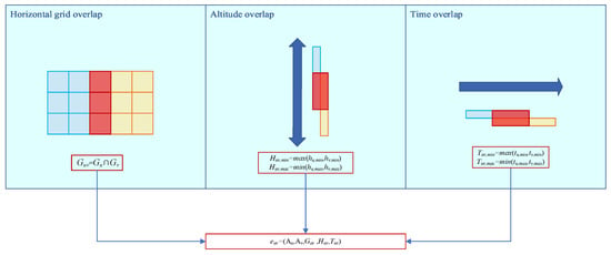
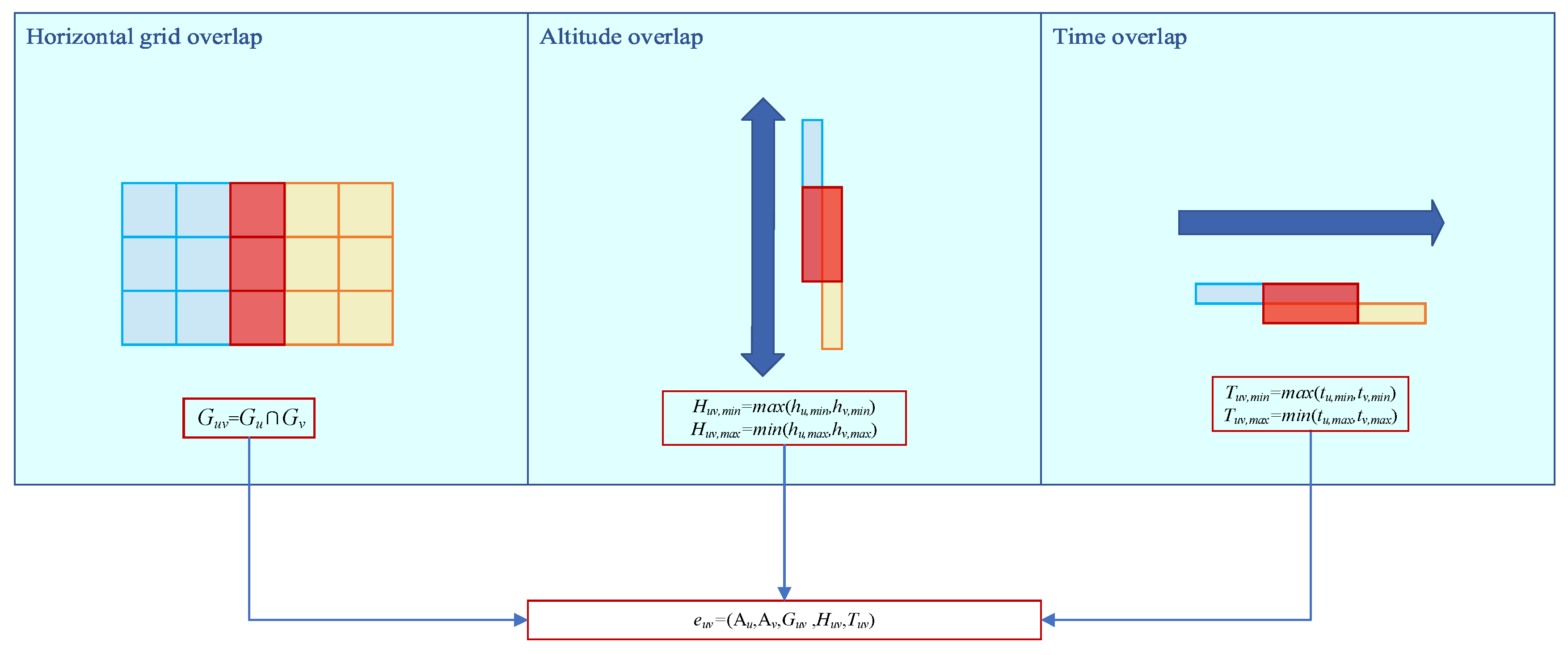
The conflict-event set detected during the ad hoc implementation phase is

$$E^n=\{e_{uv}\mid I_{uv}=1,(A_u,A_v)\in C^n\}$$

(19)

where each conflict event is recorded as

$$e_{uv}=\left(A_u,A_v,G_{uv},H_{uv},T_{uv}\right)$$

(20)

With $G_{\mathit{uv}}, H_{\mathit{uv}}, T_{\mathit{uv}}$ denoting the horizontal, altitude, and time overlap regions, respectively, as illustrated in Figure 4.

Figure 4. Composition of a four-dimensional conflict event based on horizontal, altitude, and time overlaps. Blue and yellow denote the two objects, and red denotes their overlap. The vertical double-headed blue arrow indicates the altitude axis, and the horizontal blue arrow indicates the time axis.

Based on $E^n$, the conflict-related local subset of existing airspace objects is defined as

$$A{S}_c^0=\left\{\left.A_i^0\in A{S}^0\left|A_r^n\in A{S}^n,e_{ir}\in E^n\right.\right\}\right.$$

(21)

Objects in $A{S}_c^0$ are not adjusted by default, and are only allowed to participate in limited coordination when conflicts cannot be resolved by adjusting newly inserted objects alone. All remaining existing objects

$$A{S}_f^0=A{S}^0\backslash A{S}_c^0$$

(22)

remain unchanged throughout the ad hoc implementation phase.

$$P^{loc}=(A_i^0,A_v)|A_i^0\in A{S}_c^0,A_v\in \mathcal{N}(A_i^0)\cap A_{fixed}$$

(23)

where $\mathcal{N}(A_i^0)$ denotes the neighboring existing airspace objects around $A_i^0$. $\mathcal{N}(A_i^0)$ is obtained from the GeoSOT cell codes of $A_i^0$ by a one-level prefix expansion: each occupied code c is expanded by its proper prefixes and by truncation of the last $b=1$ character ($b=1$ in all experiments). $P^{loc}$ then contains the pairs $(A_i^0,A_v)$ with $A_i^0\in A{S}_c^0$ and $A_v\in \mathcal{N}(A_i^0)\cap A_{fixed}$. This neighborhood is used only to construct the local validation set $P^{loc}$. It is a search/validation window, not an operational separation buffer; operational protection is already embedded in the occupancies of Section 2.1 and Section 2.2. This local validation set avoids global conflict detection among all existing airspace objects while ensuring that local adjustment does not compromise the safety of the baseline plan [11].

The four-dimensional discretization model established in this section transforms conflict detection into one-dimensional code matching and interval comparison [10]. Its output, the standardized conflict-event set $E^n$, serves as the direct input to the resolution model developed in Section 3. The main symbols used in this section are summarized in Table 2.

Table 2. Main notation for existing and newly inserted airspace objects.

Symbol	Meaning
Ai0	Existing (baseline) airspace object
Ai(0,new)	Existing object after Stage-2 local coordination
Arn	Newly inserted (ad hoc) airspace object
Ar(n,new)	Ad hoc object after adjustment
xrn, xi0	Seven-dimensional adjustment vectors of the ad hoc and existing objects
Fn, F0	Offset/shrink transformation of an ad hoc object and of an existing object
ASc0	Conflict-related subset of existing objects eligible for limited coordination
Ploc	Local validation pairs in a grid neighborhood of an existing object (not an operational buffer)
$\mathcal{N}(A_i^0)$	Neighborhood of $A_i^0$ used to build $P^{loc}$: GeoSOT codes expanded by $b=1$ prefix level.

3. Conflict Resolution Model for Ad Hoc Airspace Insertion

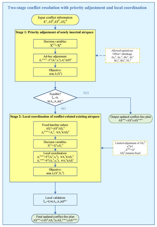
Conflict resolution during the ad hoc implementation phase differs fundamentally from the global optimization performed in the pre-planning stage: the existing baseline airspace plan must be protected from global re-optimization, and newly inserted objects are adjusted with priority. If conflicts can be resolved by adjusting newly inserted objects alone, all existing objects remain unchanged. Only when no feasible first-stage solution exists is a small, conflict-related subset of existing objects allowed to participate in limited coordination at a substantially higher adjustment cost, while all other existing objects remain fixed.

In the online implementation, failure to obtain a feasible Stage-1 solution within the prescribed computational budget does not, by itself, prove that the Stage-1 subproblem is mathematically infeasible. Accordingly, Stage 2 may also be activated as a computational fallback when the Stage-1 search terminates without certifying a feasible solution. The two cases—proven infeasibility and no feasible solution found within the computational budget—are recorded separately.

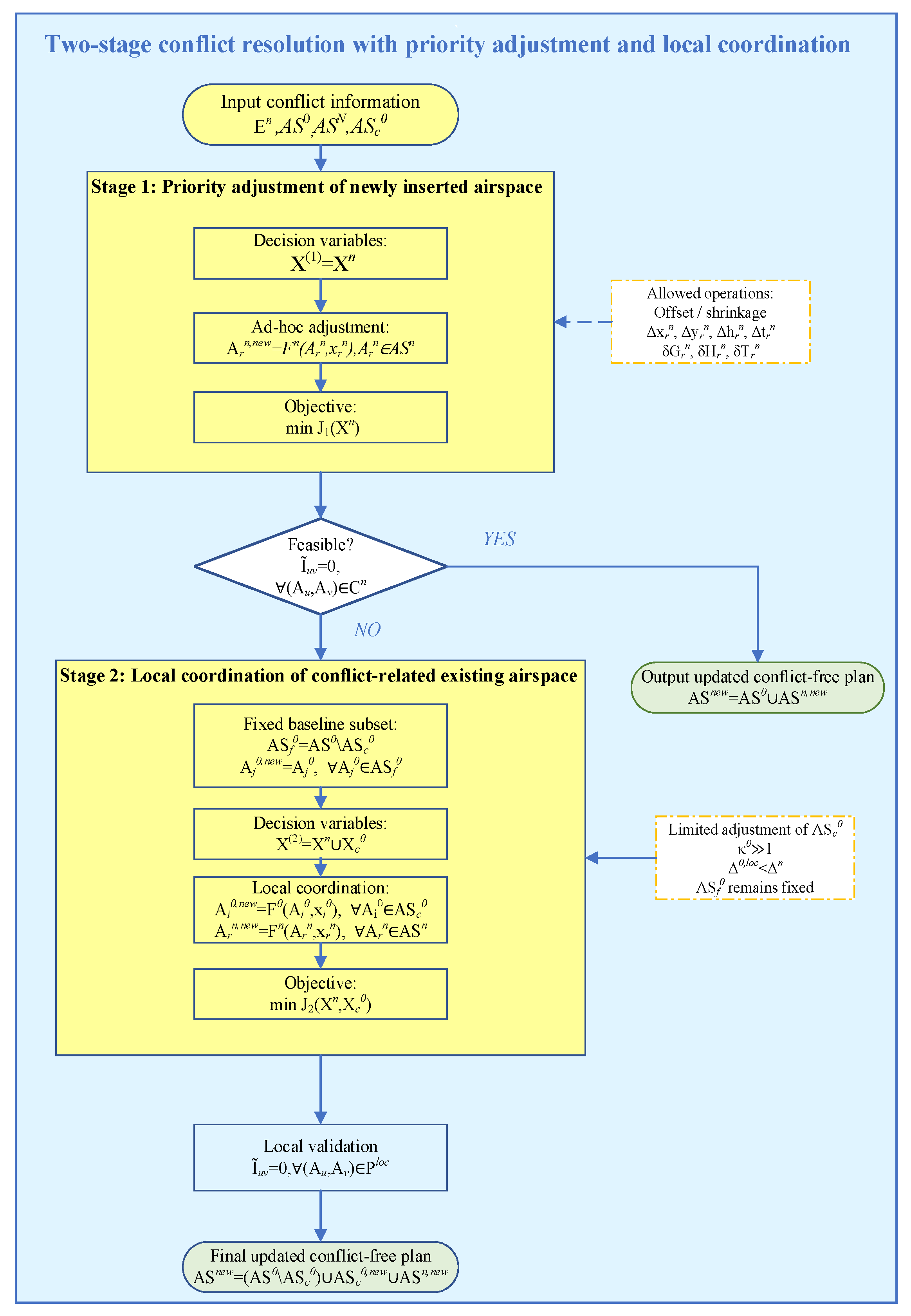
This section formulates the corresponding local incremental optimization problem in five parts: Section 3.1 defines the decision variables; Section 3.2 specifies the adjustment constraints; Section 3.3 defines the two underlying adjustment mechanisms—offset and shrinkage—as shape- and strategy-independent operational primitives; Section 3.4 specifies the two-stage priority-adjustment and local-coordination strategy that governs when, and on which objects, these mechanisms are invoked; and Section 3.5 gives the unified objective function. The overall resolution logic is illustrated in Figure 5.

Figure 5. Two-stage conflict resolution mechanism for ad hoc airspace insertion under baseline-plan protection.

3.1. Definition of Decision Variables

For a newly inserted airspace object $A_r^n$, the adjustment decision variable is defined as the seven-dimensional vector

$$x_r^n=(\Delta x_r^n,\Delta y_r^n,\Delta h_r^n,\Delta t_r^n,\delta G_r^n,\delta H_r^n,\delta T_r^n)$$

(24)

where $\Delta x_r^n$, $\Delta y_r^n$ denote horizontal offsets in two directions, $\Delta h_r^n$ the altitude offset, $\Delta t_r^n$ the time-window offset, and $\delta G_r^n,\delta H_r^n,\delta T_r^n$ (≤0) the reduction amounts in horizontal area, altitude thickness, and duration, respectively. The adjusted object is

$$A_r^{n,new}=F^n(A_r^n,x_r^n)$$

(25)

By analogy, for an existing airspace object $A_i^0\in A{S}_c^0$ participating in second-stage local coordination, the decision variable $x_i^0$ takes the same seven-dimensional form, with each component sharing an identical physical meaning to its counterpart in $x_r^n$:

$$\begin{gathered} A_r^{n,new}=F^n(A_r^n,x_r^n) \\ {A}_i^{(0,new)}=F^0(A_i^0,x_i^0) \end{gathered}$$

(26)

where $F^0(·)$ is structurally identical to $F^n(·)$. The only difference lies in the allowable range and cost weight of each component, which are, respectively, much smaller and much higher than those of newly inserted objects (see Section 3.2).

The first-stage decision-variable set is

$$X^{(1)}=X^n=\{x_r^n\mid A_r^n\in A{S}^n\}$$

(27)

with all existing objects fixed, i.e., $A_i^{0,new}=A_i^0,\forall A_i^0\in A{S}^0$. If a feasible $X^{(1)}$ eliminates all conflicts, resolution ends at this stage.

If Stage 1 is infeasible, the decision-variable set is extended to

$$X^{(2)}=X^n\cup X_c^0 X_c^0=\{x_i^0\mid A_i^0\in A{S}_c^0\}$$

(28)

while objects in $A{S}_f^0$ remain fixed: $A_j^{0,new}=A_j^0,\forall A_j^0\in A{S}_f^0$.

This formulation ensures that priority is always given to adjusting newly inserted objects; existing objects are never globally re-optimized, and only a small, conflict-related subset is slightly adjusted when necessary.

In Stage 1, only newly inserted airspace objects are adjustable. The corresponding decision-variable set is

$$X^{(1)}=X^n,$$

(29)

and all existing objects remain fixed:

$$A_i^{(0,new)}=A_i^0,\forall A_i^0\in A{S}^0.$$

(30)

Let $P^{(1)}$ denote the complete Stage-1 validation set, which contains every object pair that may become conflicting under the admissible Stage-1 adjustment ranges and includes at least one newly inserted object. A Stage-1 solution is feasible if it satisfies the adjustment constraints and

$${\tilde{I}}_{uv}(X^{(1)})=0, \forall (A_u,A_v)\in P^{(1)}.$$

(31)

If such a solution is obtained, the resolution process terminates, and all existing objects remain unchanged.

In Stage 2, the decision-variable set is extended to

$$X^{(2)}=X^n\cup X_c^0,$$

(32)

where $X_c^0$ contains the decision variables of the conflict-related existing airspace subset $A{S}_c^0$. The remaining existing objects form the fixed baseline subset and satisfy

$$A_j^{(0,new)}=A_j^0, \forall A_j^0\in A{S}_f^0.$$

(33)

Let $P^{(2)}$ denote the complete Stage-2 validation set. It contains every pair that may become conflicting under the admissible Stage-2 adjustment ranges and has at least one endpoint in $A{S}^n\cup A{S}_c^0$. Therefore, $P^{(2)}$ includes potentially affected pairs between newly inserted objects, between newly inserted and existing objects, between locally coordinated existing objects, and between a locally coordinated existing object and a fixed existing object. Pairs consisting of two objects in $A{S}_f^0$ need not be re-evaluated because both objects remain unchanged and their baseline conflict-free relationship has already been established.

A Stage-2 solution is feasible if

$${\tilde{I}}_{uv}(X^{(2)})=0, \forall (A_u,A_v)\in P^{(2)}.$$

(34)

Objects in $A{S}_f^0$ are not decision variables, but they remain fixed obstacles during conflict validation. This distinction protects the baseline plan without omitting secondary conflicts caused by the movement or shrinkage of adjustable objects.

3.2. Adjustment Constraints

The feasible regions of both stages are jointly bounded by the four types of constraints summarized in Table 3. The same constraint structure is used in both stages, but the allowable adjustment ranges and cost weights depend on the object category. Newly inserted objects use the mission-allowable offset and shrinkage ranges, whereas locally coordinated existing objects use substantially smaller adjustment ranges and substantially higher adjustment-cost weights.

Table 3. Summary of adjustment constraints for newly inserted and locally coordinated existing airspace objects.

Constraint Type	Applies to	Mathematical Form	Physical Meaning
Offset-bound	$A_r^n$	$\begin{array}{l}\left|\Delta x_r^n\right|\le \Delta x_{r,\max }^n,\left|\Delta y_r^n\right|\le \Delta y_{r,\max }^n\\ \left|\Delta h_r^n\right|\le \Delta h_{r,\max }^n,\left|\Delta t_r^n\right|\le \Delta t_{r,\max }^n\end{array}$	Offsets in all four dimensions do not exceed the mission-allowable ranges
Resource-preservation	$A_r^n$	$\begin{array}{l}{G}_r^{n,new}\ge G_{r,min}^n,H_r^{n,new}\ge H_{r,min}^n,\\ T_r^{n,new}\ge T_{r,min}^n\end{array}$	Shrunk resources still satisfy minimum mission requirements
Available-airspace	$A_r^n,A_i^0$	$\begin{array}{l}{H}^{new}\subseteq H_{avail},G^{new}\subseteq G_{avail},\\ T^{new}\subseteq T_{avail}\end{array}$	Adjusted objects remain within the available horizontal, altitude, and time domains.
Local-adjustment-bound (Stage 2 only)	$A_i^0\in A{S}_c^0$	$\begin{array}{l}\left|\Delta x_i^0\right|\le \Delta x_{i,\max }^0,\dots ,\left|\Delta t_i^0\right|\le \Delta t_{i,\max }^0;\\ \Delta {\left(·\right)}_{i,\max }^0\le \Delta {\left(·\right)}_{r,\max }^n\end{array}$	Local adjustment range of existing objects is far smaller than that of newly inserted objects
Baseline protection	$A_j^0\in A{S}_f^0$	$A_j^{0,new}=A_j^0$	Objects outside the conflict-related subset remain fixed

In addition, the cost weight assigned to a locally coordinated existing object is set substantially higher than that assigned to a newly inserted object:

$$w_i^0\gg w_r^n, \forall A_i^0\in A{S}_c^0,A_r^n\in A{S}^n$$

(35)

which ensures that the model always gives priority to adjusting newly inserted ad hoc airspace objects rather than disturbing the conflict-free plan established in the pre-planning stage.

$$w_i^0=\gamma w_r^n, \gamma >1,$$

(36)

$$\forall A_i^0\in A{S}_c^0, A_r^n\in A{S}^n.$$

(37)

The higher weight discourages unnecessary modification of existing objects within Stage 2. However, the strict priority of adjusting newly inserted objects is imposed primarily by the two-stage decision structure: Stage 1 permits only newly inserted objects to be adjusted, and Stage 2 is activated only if the Stage-1 subproblem is proven infeasible or if the online Stage-1 search terminates without certifying a feasible solution within its prescribed computational budget.

3.3. Underlying Adjustment Mechanisms: Offset and Shrinkage

Regardless of which object—newly inserted or locally coordinated existing—is being adjusted, only two types of operational primitives are used: offset and shrinkage. These mechanisms are defined independently of any resolution strategy or search algorithm, and constitute shared, callable operations invoked by both stages of the strategy in Section 3.4, as well as by the online search algorithm developed in Section 4.

Offset mechanism. For an object $A$ with grid set $G$, altitude interval $H=\left[h_{\min },h_{\max }\right]$, and time window $T=\left[t_{\min },t_{\max }\right]$, the horizontal offset is

$$G^{new}=T_h(G_r^n,\Delta x_r,\Delta y_r)$$

(38)

the altitude offset is

$$H^{new}=[h_{min}+\Delta h, h_{max}+\Delta h]$$

(39)

and the time offset is

$$T^{new}=[t_{min}+\Delta t, t_{max}+\Delta t]$$

(40)

where $T_h\left(·\right)$ denotes the horizontal grid-shifting function.

Shrinkage mechanism. The altitude and time dimensions follow an identical center-preserving shrinkage formulation. Using a unified symbol $\xi \in \{h,t\}$ to denote either dimension,

$${\xi }_{center}={\displaystyle \frac{{\xi }_{\min }+{\xi }_{\max }}{2}}, {\xi }_{width}^{new}={\xi }_{width}+\delta \xi \left(\delta \xi \le 0\right)$$

(41)

$${\xi }^{new}=\left[{\xi }_{center}-{\displaystyle \frac{1}{2}}{\xi }_{width}^{new},{\xi }_{center}+{\displaystyle \frac{1}{2}}{\xi }_{width}^{new}\right]$$

(42)

This single formulation applies to both altitude shrinkage $\left(\xi =h\right)$ and time shrinkage $\left(\xi =t\right)$, voiding duplicate derivations.

Horizontal-area shrinkage depends on the object’s geometric shape and is performed by a shape-aware grid-shrinkage function,

$$G_r^{n,new}=\mathsf{\Psi }(G,\delta G,shape)$$

(43)

which allocates the reduced grid count between the two horizontal directions according to the object’s bounding-box aspect ratio—e.g., proportional allocation for near-circular shapes, and long-axis-priority allocation for corridor-type shapes—ensuring that the resulting shape remains geometrically feasible.

Separation conditions. After adjustment, a conflict pair $\left(A_u,A_v\right)$ is considered resolved if the objects are separated in at least one dimension. These conditions restore exclusivity of the protected occupancies in Section 2. They do not introduce a second, aircraft-centric separation standard:

$$G_u^{new}\cap G_v^{new}=\varnothing or H_u^{new}\cap H_v^{new}=\varnothing or T_u^{new}\cap T_v^{new}=\varnothing$$

(44)

equivalently, using the indicator functions defined in Section 2.3,

$$I_{uv}^{new}=I_{uv}^{G,new}\cdot I_{uv}^{H,new}\cdot I_{uv}^{T,new}=0$$

(45)

Together with their separation conditions, the offset and shrinkage mechanisms constitute the complete set of operational primitives available to any resolution strategy or search procedure. They do not themselves determine which object, dimension, or magnitude to adjust—this decision is governed by the strategy described next.

Both offset and shrinkage alter the occupied region of an airspace object. Consequently, after either mechanism is applied, conflict indicators are recomputed using the updated horizontal, altitude, and time regions of the affected objects. The initially detected conflict set is used to guide the search, but it is not treated as a fixed or exhaustive validation set. All potentially affected pairs incident to an adjusted object are re-evaluated within the corresponding stage-specific validation set $P^{(1)}$ or $P^{(2)}$.

3.4. Two-Stage Priority-Adjustment and Local-Coordination Strategy

Building on the mechanisms defined in Section 3.3, this section specifies how, and on which objects, these mechanisms are invoked across the two resolution stages. The strategy protects the existing baseline plan through a strict stage priority rather than through adjustment-cost weighting alone [15].

Stage 1 (priority adjustment). Only newly inserted objects are eligible for adjustment. The Stage-1 decision-variable set is

$$X^{(1)}=X^n$$

(46)

For every potentially affected pair involving at least one newly inserted object, the offset and/or shrinkage mechanisms defined in Section 3.3 are invoked on $A_r^n$, subject to the constraints in Table 3. Conflict validation is performed over the complete Stage-1 validation set $P^{(1)}$, rather than only over the initially detected conflict set $C^n$. Stage 1 therefore searches for a feasible $X^{(1)}$ such that

$${\tilde{I}}_{uv}(X^{(1)})=0, \forall (A_u,A_v)\in P^{(1)}.$$

(47)

If such a solution is found, the resolution process terminates, and all existing objects remain unchanged. The resulting updated plan is

$$A{S}^{new}=A{S}^0\cup A{S}^{(n,new)}.$$

(48)

Stage 2 (local coordination). If the Stage-1 subproblem is proven infeasible, the same offset and shrinkage mechanisms are additionally invoked on the conflict-related existing airspace subset $A{S}_c^0$ but under substantially tighter adjustment bounds and substantially higher adjustment-cost weights. In the time-budgeted online implementation, Stage 2 may also be activated if the Stage-1 search terminates without certifying a feasible solution within the prescribed computational budget. This search outcome is treated as uncertified within budget and is not interpreted as proof of mathematical infeasibility.

The Stage-2 decision-variable set is

$$X^{(2)}=X^n\cup X_c^0.$$

(49)

For every $A_i^0\in A{S}_c^0$, local coordination is represented by

$$A_i^{(0,new)}=F^0(A_i^0,x_i^0),$$

(50)

Whereas every object outside the conflict-related subset remains fixed:

$$A{S}_f^0=A{S}^0\backslash A{S}_c^0,$$

(51)

$$A_j^{(0,new)}=A_j^0, \forall A_j^0\in A{S}_f^0.$$

(52)

Newly inserted objects remain adjustable in Stage 2:

$$A_r^{(n,new)}=F^n(A_r^n,x_r^n), \forall A_r^n\in A{S}^n.$$

(53)

Stage-2 conflict validation is performed over $P^{(2)}$, which contains all potentially affected pairs having at least one endpoint in $A{S}^n\cup A{S}_c^0$. Accordingly, Stage 2 requires

$${\tilde{I}}_{uv}(X^{(2)})=0, \forall (A_u,A_v)\in P^{(2)}.$$

(54)

Although objects in $A{S}_f^0$ remain fixed, potentially affected pairs between $A{S}_f^0$ and $A{S}^n\cup A{S}_c^0$ are retained in $P^{(2)}$. Only pairs whose two endpoints both belong to $A{S}_f^0$ are excluded from re-evaluation, because neither object changes and their baseline conflict-free relationship has already been established.

If Stage 2 is activated because the Stage-1 search result is uncertified, rather than because Stage-1 infeasibility has been proven, a Stage-2 solution that adjusts only newly inserted objects remains admissible and is preferred to any solution that modifies an existing object. Entering Stage 2 therefore does not imply that an existing object must be adjusted.

The final updated conflict-free plan is

$$A{S}^{new}=(A{S}^0\backslash A{S}_c^0)\cup A{S}_c^{(0,new)}\cup A{S}^{(n,new)}.$$

(55)

This two-stage strategy reuses the same underlying mechanisms consistently across both stages while protecting the baseline plan by construction. Existing objects are adjusted only in Stage 2, only within $A{S}_c^0$ and only within strictly bounded margins. Objects in $A{S}_f^0$ remain unchanged but are retained as fixed obstacles during conflict validation.

3.5. Objective Function and Unified Model

The total adjustment cost combines an offset cost and a shrinkage cost, each normalized by its corresponding maximum allowable range and weighted by the object-specific adjustment-cost weight. For any adjusted object A, whether newly inserted or locally coordinated, with cost weight $w_A$,

$$J_{offset(A)}=w{\displaystyle \sum _{\xi }\frac{\left|\Delta \xi \right|}{{\xi }_{max}}}, J_{shrink(A)}=w{\displaystyle \sum _{\xi }\frac{\left|\delta \xi \right|}{{\xi }_{max}^{shrink}}}$$

(56)

The system-level objective is the weighted sum over all adjusted objects,

$$J=\lambda {\displaystyle \sum _A{J}_{offset(A)}}+(1-\lambda ){\displaystyle \sum _A{J}_{shrink(A)}}$$

(57)

where $\lambda \in [0,1]$ balances the preference between offset and shrinkage: a larger $\lambda$ favors horizontal, altitude, or temporal translation, whereas a smaller $\lambda$ favors resource compression. The adjustment cost $J$ is minimized within each activated stage. The strict preference for leaving existing objects unchanged is determined by the two-stage activation rule and is not approximated solely through the magnitude of the existing-object cost weight.

Combining Section 3.1, Section 3.2, Section 3.3 and Section 3.4, the conflict-resolution problem for ad hoc airspace insertion is formulated stage by stage as

$$\underset{X^n}{\min imize }{J}_1(X^n)$$

(58)

subject to the constraints in Table 3 and

$${\tilde{I}}_{uv}(X^{(1)})=0, \forall (A_u,A_v)\in P^{(1)}.$$

(59)

for Stage 1, where

$$X^{(1)}=X^n.$$

(60)

If Stage 1 is proven infeasible, or if the time-budgeted Stage-1 search terminates without certifying a feasible solution, Stage 2 solves

$$\underset{X^n,X_c^0}{minimize }{J}_2(X^n,X_c^0)$$

(61)

subject to the constraints in Table 3,

$$A_j^{(0,new)}=A_j^0, \forall A_j^0\in A{S}_f^0,$$

(62)

And

$${\tilde{I}}_{uv}(X^{(2)})=0, \forall (A_u,A_v)\in P^{(2)}.$$

(63)

where

$$X^{(2)}=X^n\cup X_c^0.$$

(64)

To express the strict stage priority in a unified form, define

$$z_0=\left\{\begin{array}{c}0, x_i^0, \forall A_i^0\in A{S}_c^0,\hfill \\ 1, otherwise\hfill \end{array}\right.$$

(65)

The unified priority rule can then be written as

$$\underset{X^{(2)}}{lexmin}(z_0,J),$$

(66)

subject to the Stage-2 feasibility and adjustment constraints.

The first lexicographic component prefers every feasible solution that leaves all existing objects unchanged over every solution that adjusts at least one existing object. The second component minimizes the original adjustment cost J within the selected category. Thus, the original cost function is retained, while the priority of adjusting newly inserted objects is enforced explicitly by the stage structure.

For an exact optimization method, the lexicographic formulation is equivalent to first solving Stage 1 and activating Stage 2 only if Stage 1 is infeasible. For the time-limited online algorithm developed in Section 3, a failure to obtain a Stage-1 feasible solution within the prescribed budget is reported as an uncertified search result unless infeasibility is established separately.

This unified, priority-driven and cost-based model, together with the offset and shrinkage mechanisms defined in Section 3.3, provides the mathematical basis for the online search algorithm developed in Section 4. The adjustment actions generated by that algorithm are direct instantiations of the mechanisms defined in Section 3.3, while the two-stage activation logic and priority ordering follow the strategy defined in Section 3.4.

The decision variables, constraints, and objective are related as follows. The decision variables are the seven-dimensional offset/shrink vectors $x_r^n$ for newly inserted objects and, when Stage 2 is activated, $x_i^0$ for locally coordinated baseline objects (Section 3.1). Feasible values of these vectors are restricted by the offset bounds, resource-preservation limits, available-airspace membership, and Stage-2 local-adjustment bounds in Table 3, together with the occupancy-conflict indicators of Equations (15)–(18) on the complete stage-wise validation set. The scalar cost $J$ in Equations (56) and (57) is the objective: it is minimized only after the lexicographic Stage-1/Stage-2 rule has selected the admissible object set. In short, the variables propose an occupancy, the constraints certify whether it is conflict-free, and $J$ ranks certified candidates.

The proposed model is a discrete combinatorial problem over grid-code sets and interval attributes. It is not formulated as a standalone mixed-integer linear program (MILP). Section 4 solves it online with IAO-TPTS. The MILP solver used in Section 5.4 is a comparison baseline only; it is not the main contribution of this paper.

4. IAO-TPTS Algorithm

Section 4 instantiates the Stage-1/Stage-2 policy of Section 3.4 under a hard wall-clock budget. Incremental Ad hoc Operation–Tiered Priority Time-Sliced Search (IAO-TPTS) is the main scheduling algorithm, whereas Dimension-wise Conflict-Driven Assignment (DCDA) and Hybrid Adaptive Large Neighborhood Search (Hybrid-ALNS) are phase-specific search operators. All candidate moves use the offset and shrink primitives of Section 3.3, the tier bounds and β-protection weight asymmetry of Table 3, and the objective $J$ defined in Section 3.5.

The inputs are the ad hoc object set $A{S}^n$, baseline object set $A{S}^0=A{S}_f^0\cup A{S}_c^0$ with the locally adjustable subset $A{S}_c^0$, the candidate conflict-event set $E^n$, the local validation set $P^{loc}$, the total wall-clock budget $T_{total}$, and the Phase-A sub-budget $T_A$. The default values are $T_{total}=180 \mathrm{s}$ and $T_A=20 \mathrm{s}$. A small validation reserve $T_{val}$ is retained from the total budget for final certification.

4.1. Overview

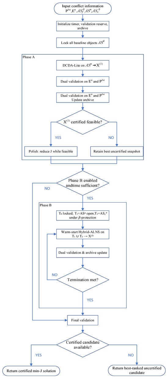
IAO-TPTS implements the two-stage policy online. Phase A locks all baseline objects and searches for feasibility by modifying only $A{S}^n$, thereby realizing $X^{(1)}=X^n$ of Section 3.4. Phase B uses the remaining budget to refine the Phase-A result on a tiered neighborhood in which both $A{S}_c^0$ may be modified, realizing $X^{(2)}=(X^n,X_c^0).$

IAO-TPTS is therefore not a third solver running in parallel with DCDA-Lite and Hybrid-ALNS. It only controls their execution order, time allocation, adjustable object sets, validation, and best-so-far selection. Phase B is invoked after Phase A whenever sufficient time remains. If Phase A has already certified a Stage-1 feasible solution, Phase B performs T1-only objective polishing with all T2 baseline objects kept locked. T2 objects are unlocked only when Phase A does not certify Stage-1 feasibility.

4.2. Dual Validation and Solution Ranking

For any candidate adjustment $X$, let $I_{uv}^{new}(X)$ denote the pairwise conflict indicator of Section 2.3 for the ordered pair $(u,v)$. A candidate is certified only after passing two validation gates:

$$Feasible(X)\rightleftharpoons I_{uv}^{new}(X)=0,\forall (u,v)\in E^n\cup P^{loc}.$$

(67)

Equivalently,

$$Feasible(X)\rightleftharpoons {\mathsf{\Phi }}_{E_n}(X)=\varnothing \wedge {\mathsf{\Phi }}_{P^{loc}}(X)=\varnothing ,$$

(68)

where ${\mathsf{\Phi }}_{E^n}\left(X\right)$ and ${\mathsf{\Phi }}_{P^{loc}}(X)$ collect unresolved conflict pairs in $E^n$ and $P^{loc}$, respectively. The second gate prevents an adjustment from resolving an original conflict while introducing a nearby secondary conflict. The “complete stage-wise validation set” in Table 1 is $V_{\mathrm{stage}}$. It is the same pair set used in Equations (67) and (68) and Algorithm 1: $V_{\mathrm{stage}}=E^n\cup P^{loc}$. $E^n$ contains every pair with at least one newly inserted object (the Stage-1 set of Section 3.4). $P^{loc}$ contains local pairs between a coordinated baseline object and a neighboring fixed object (Equation (23)). Stage 1 uses $E^n$ ($P^{loc}=\varnothing$ because no baseline object moves). Stage 2 uses $E^n\cup P^{loc}$.

Algorithm 1. Incremental Ad hoc Operation Tiered Priority Time-Sliced Search

1. Input: $A{S}^n$, $A{S}_f^0$, $A{S}_c^0$, $E^n$, $P^{loc}$, Table 3 bounds and $\beta$, $T_{total}$, $T_A$. 2. Initialize the timer, the validation reserve $T_{val}$, and the empty candidate archive. 3. Lock all objects in $A{S}^0$ and permit moves only on $A{S}^n$. 4. Run DCDA-Lite until Phase-A termination or $T_A^{\prime }$ is reached; validate each new candidate on $E^n\cup P^{loc}$ and update the archive; denote the incumbent by $X^{(1)}$. 5. If $X^{(1)}$ is certified feasible and polishing is enabled: reduce its nonzero components by ten percent while feasibility holds and $J$ decreases. 6. If Phase B is enabled and the remaining time is sufficient: 6.1 If Phase A certified a Stage-1 feasible solution: keep all baseline objects (including $A_{\mathrm{local}}$ locked; searchable set = ad hoc (T1) only. Else: keep $A_{fixed}$ locked; unlock $A_{local}$ (T2) under Table 3 bounds and β-protection; $searchable set = ad-hoc\cup A_{\mathrm{local}}$. 6.2 Warm-start Hybrid-ALNS from the Phase-A incumbent over the searchable set. 6.3 Dual-validate each accepted candidate and update the archive by $rank(x)=(z^0,{\delta }_{feas},\left|C\right|,J)$ 7. Stop when the deadline is reached or no admissible improvement remains. 8. Perform final validation within the reserved time $T_{val}$. 9. Return: tthe certified archive candidate of minimum lexicographic $(z^0,\left|C\right|,J)$; if none is certified, return the highest-ranked uncertified candidate.

Every fully validated snapshot is stored in an archive and compared by

$$\begin{gathered} rank(x)=(z^0,{\delta }_{feas},\left|C\right|,J) \\ {z}_0=\left\{\begin{array}{c}1, \mathit{if} \mathit{any} T2(A_{\mathit{local}}) \mathit{object} \mathit{is} \mathit{translated} \mathit{or} \mathit{shrunk}\hfill \\ 0, otherwise\hfill \end{array}\right. \\ {\delta }_{\mathit{feas}}=\left\{\begin{array}{c}0, \mathit{if} dual-validated \mathit{feasible}\hfill \\ 1, otherwise\hfill \end{array}\right. \end{gathered}$$

(69)

Equation (69) is applied only after a feasibility filter. Certified candidates (${\delta }_{feas}=0$) are considered first and are ranked by $(z^0,\left|C\right|,J)$: any certified candidate with $z^0=0$ is strictly preferred to any certified candidate with $z^0=1$, independently of $J$. Uncertified candidates are ranked among themselves only when the archive contains no certified solution. An infeasible candidate with $z^0=0$ is never selected over a feasible candidate with $z^0=1$. Only candidates that have passed both validation gates in Equations (67) and (68) may replace a certified incumbent.

4.3. Phase A: Ad Hoc-Only Fast Feasibilization (DCDA-Lite)

Phase A realizes Stage 1 by locking every object in $A{S}^0$, including $A{S}_c^0$, and by permitting adjustments only on $A{S}^n$. It invokes DCDA-Lite, the ad hoc-restricted implementation of DCDA, within

$$T_A^{\prime }=min(T_A,T_{total}-T_{val}).$$

(70)

DCDA-Lite processes unresolved conflict pairs in $E^n$ sequentially. For each pair, it evaluates admissible horizontal, altitude, temporal, and shrink actions and applies the action with the lowest marginal cost that improves the conflict state. During iterative search, conflict rechecking is scoped to pairs in $E^n$ involving an affected ad hoc object. A candidate is nevertheless accepted only after complete dual validation on $E^n\cup P^{loc}$.

If Phase A certifies a Stage-1 solution $X^{(1)}$ and time remains, each nonzero component of $X^{(1)}$ is reduced by ten percent in turn. A reduction is retained only when both validation gates remain satisfied and $J$ decreases. Failure to certify feasibility within $T_A^{\prime }$ is reported as an uncertified result within budget, consistent with Section 3.4, rather than as a proof of infeasibility.

4.4. Phase B: Tiered Refinement (Hybrid-ALNS)

Phase B realizes Stage 2 with the remaining budget after Phase A and the validation reserve. Unlocking T2 is conditional. If Phase A has certified Stage-1 feasibility, Phase B does not unlock $A_{local}$. Hybrid-ALNS refines only T1. If Stage-1 is uncertified, T2 is unlocked under Table 3 and

β-protection, and Hybrid-ALNS searches over ad hoc objects and $A_{local}$.

The objects are partitioned into three tiers:

$$T_0=A{S}_f^0, T_1=A{S}^n, T_2=A{S}_c^0.$$

(71)

Objects in $T_0$ remain permanently fixed as required by Section 3.4. Objects in $T_1$ retain their Section 3.3 primitives without additional restriction, while objects in $T_2$ are unlocked only under the tight bounds and the $\beta$ protection weight asymmetry defined in Table 3 and Section 3.2. The asymmetric weighting makes any modification of a $T_2$ object substantially more costly in $J$ than an equivalent modification of a $T_1$ object, so baseline coordination is triggered only when ad hoc-only adjustment is insufficient.

Hybrid-ALNS is warm-started from the best Phase-A snapshot $X^{(1)}$ and searches over $T_1\cup T_2$ to produce $X^{(2)}$. Its original destroy-repair operators, guided repair, and simulated-annealing acceptance rule are retained; IAO-TPTS supplies only the tier restrictions, protected bounds, deadline, and warm-start incumbent. Conflict rechecking remains limited to $E^n\cup P^{loc}$.

Validated candidates are continuously inserted into the archive according to the ranking rule of Section 4.2.

4.5. Termination, Best-So-Far Selection, and Ablation

The procedure terminates upon normal Phase-B completion, exhaustion of the global deadline, or detection that the remaining time is insufficient for another search step together with final validation. Search stops before the validation reserve is consumed. The output is the certified archive candidate of minimum lexicographic $(z^0,\left|C\right|,J)$; if none exists, the highest-ranked uncertified candidate is returned with its residual-conflict status.

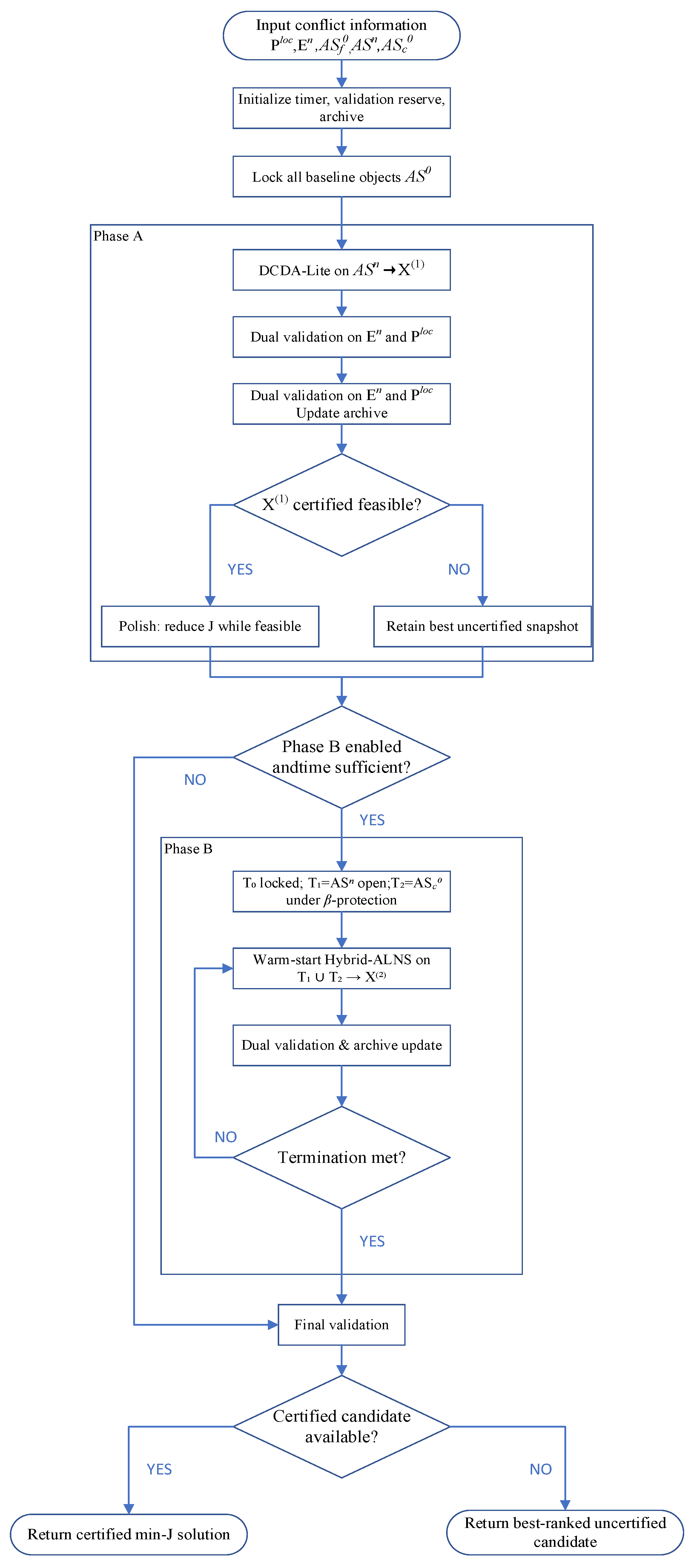
The ablation settings used in Section 5.3 disable Phase A, execute Phase A only, restrict Phase B to $A{S}^n$ without unlocking $T_2$ or disable Phase A polishing. Figure 6 summarizes the complete execution flow.

Figure 6. Execution flow of IAO-TPTS. After Phase A, T2 is unlocked only if Stage-1 is uncertified; otherwise, Phase B refines T1 only.

5. Experimental Validation

5.1. Experimental Setup

We evaluate IAO-TPTS for ad hoc airspace conflict resolution on GeoSOT adaptive grids through four experiment groups: visualization, ablation, algorithm comparison, and scalability/case analysis. All runs share the same settings: GeoSOT with L_max = 14, shape tolerance ε = 0.05; altitude 1000–8000 m; time window 08:00–18:00; total budget 180 s; baseline protection β = 20. Platforms are Windows-10-10.0.26200-SP0 and Python 3.11.15. Horizontal coordinates are WGS84 longitude and latitude. Altitude is MSL. Objects are generated as continuous protected occupancies and then mapped by Equation (11). Online detection uses only Equations (15)–(18); no additional separation buffer is applied during detection or resolution.

Comparison runs use Small/Medium/Large random scenarios with 10 instances each. Ablation uses Medium stress instances (30 seeds, variants V0–V4). Scalability fixes 10 ad hoc airspaces and varies baseline count from 20 to 300 (10 instances per level). Conflict detection uses incremental P_adhoc instead of all pairwise checks. Table 4 reports the reduction from full pairwise checks to incremental P_adhoc pairs.

Table 4. P_adhoc detection scale by scenario.

Scenario	Airspaces	Full Pairs	P_Adhoc Pairs	Reduction (%)
small	16.10 ± 1.79	123.0 ± 29.3	1.10 ± 0.32	99.10 ± 0.15
medium	48.50 ± 6.87	1173.1 ± 326.8	4.80 ± 1.23	99.57 ± 0.12
large	82.30 ± 4.92	3356.4 ± 402.9	13.80 ± 3.29	99.58 ± 0.11

5.2. Visualization

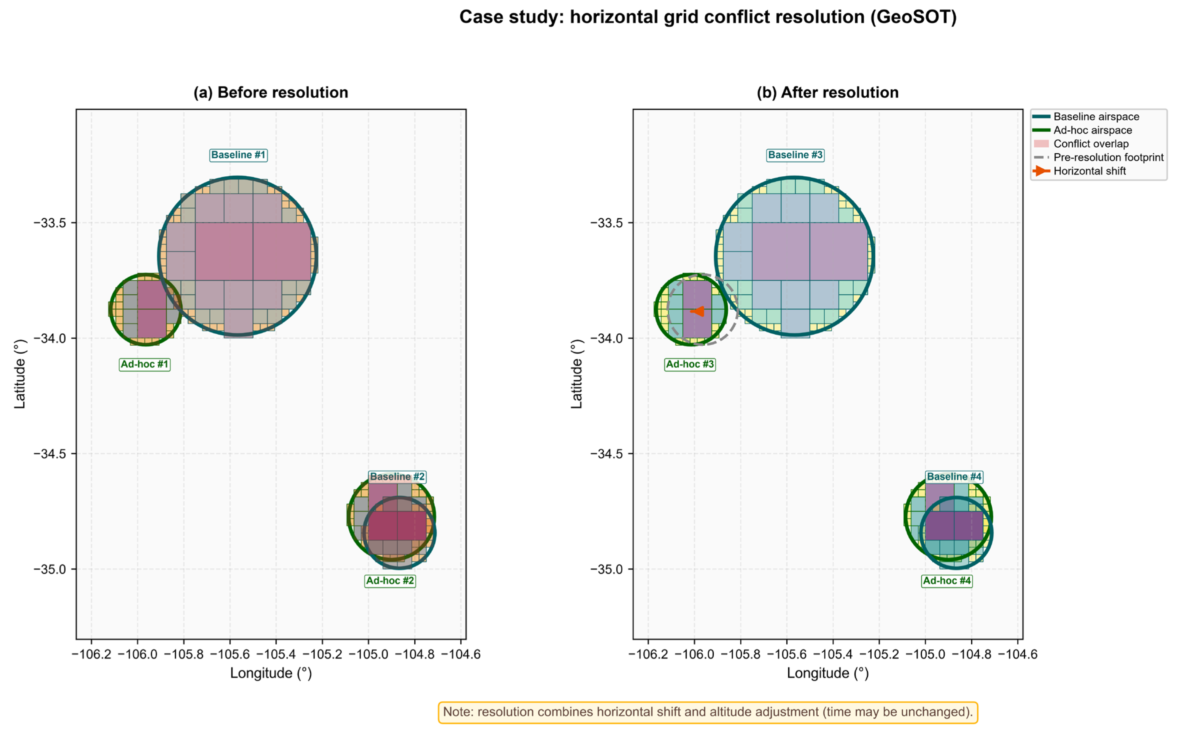
Visualization qualitatively illustrates 4D conflict resolution on GeoSOT grids. The display scenario has 32 baseline and five ad hoc airspaces; one seed was selected for clear grid changes. Horizontal panels plot only airspaces in P_adhoc conflict pairs (neighborhood focus, not the full scene). This instance has two conflict pairs and four displayed airspaces—different from the average conflict count in Medium-scale statistics.

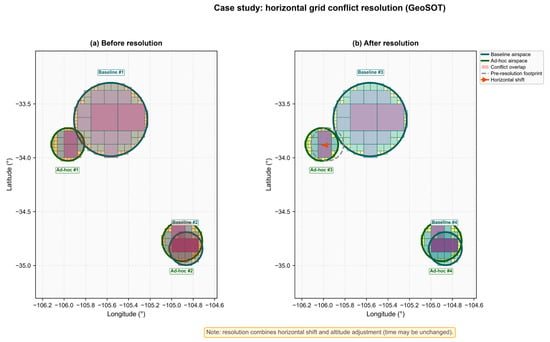
Figure 7 illustrates horizontal grid-based resolution on GeoSOT. Before resolution, conflict cells (red) occur in the overlap region between ad hoc and baseline airspaces. After resolution, the ad hoc regions are translated horizontally away from the conflict zone; the dashed outline marks the pre-resolution footprint, and the orange arrows indicate the displacement direction.

Figure 7. Horizontal grid conflict resolution (GeoSOT). Residual pink cells in (b) remain horizontally overlapping and are separated in altitude.

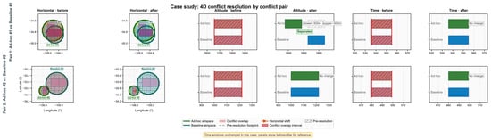
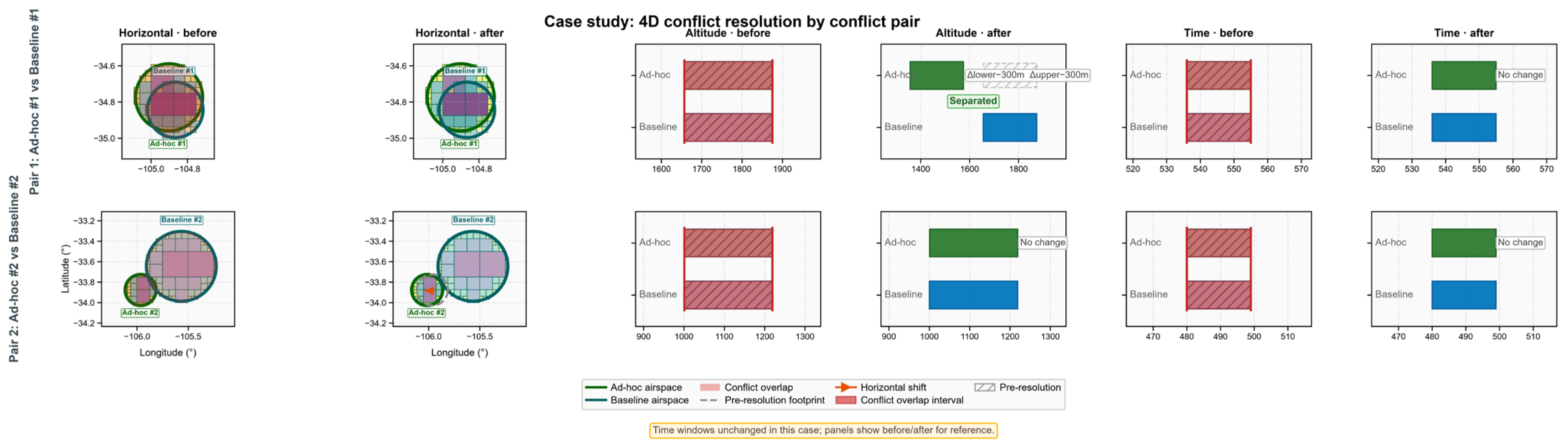
Figure 8 presents the four-dimensional resolution dashboard by conflict pair. Pair 1 is resolved primarily through altitude separation, with Δlower = Δupper = −300 m, while the horizontal footprint and time window remain unchanged. Pair 2 is resolved by horizontal translation, with no change in altitude or time.

Figure 8. Case study: 4D conflict resolution by conflict pair. Columns show the horizontal, altitude, and time views before and after resolution. Green denotes ad-hoc airspace and teal denotes baseline airspace; pink/red marks conflict overlap. Pair 1 is resolved by altitude separation; Pair 2 is resolved by a horizontal shift.

These results demonstrate that IAO-TPTS can integrate horizontal shift, altitude adjustment, and grid refinement within a unified 4D resolution framework. Under the tiered policy, T1 ad hoc airspaces are adjusted first, whereas T2 baseline airspaces remain protected by β and are not displaced in this case.

5.3. Ablation Study

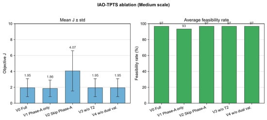
Ablation was run on Medium-scale stress instances (n = 30 seeds) where Phase A alone is often insufficient. Variants are V0 (full), V1 (Phase A only), V2 (skip Phase A), V3 (no T2 baseline move), and V4 (no dual validation). Table 5 and Figure 9 summarize the results.

Table 5. Ablation summary of IAO-TPTS (Medium scale, n = 30).

Variant	Feas. Rate (%)	Phase B (%)	T2 Mod. Rate (%)	Stage-1 Pure Rate (%)	T2 Unlock Rate (%)	Mean J	Std J	Time (s)
V0 Full	96.7	100.0	0.0	100.0	6.7	1.9454	1.1341	7.193
V1 Phase-A only	93.3	0.0	0.0	100.0	0.0	1.8580	1.0506	1.471
V2 Skip Phase-A	96.7	100.0	76.7	23.3	100.0	4.0656	2.5345	0.323
V3 w/o T2	96.7	100.0	0.0	100.0	0.0	1.9454	1.1341	7.193
V4 w/o dual val.	96.7	100.0	0.0	100.0	6.7	1.9454	1.1341	7.194

Note: T2 modification rate: percentage of runs with z0 = 1 (at least one locally coordinated baseline object translated or shrunk). Stage-1 pure rate: percentage of runs with z0 = 0. T2 unlock rate: percentage of runs in which Phase B opened A_local. Mean J is computed over feasible runs. n = 30 Medium-scale instances.

Figure 9. IAO-TPTS ablation (Medium scale). (Left): mean objective J with one standard deviation. (Right): average feasibility rate. V2 (skip Phase A) degrades J; V1 (Phase A only) reduces feasibility; V0 and V3 coincide because certified Stage-1 solutions keep z0 = 0.

The results lead to three main observations:

(1)

Phase A improves solution quality. Skipping Phase A (V2) raises mean J from 1.95 to 4.07 and increases variance (std 1.13 → 2.53). DCDA-Lite therefore remains an effective warm start: without it, Hybrid-ALNS still attains a high feasibility rate (96.7%) but at a substantially higher adjustment cost.

(2)

Phase B complements Phase A for feasibility. V1 (Phase B = 0%) yields a slightly lower mean J (1.86) among the runs it solves, but feasibility drops from 96.7% to 93.3%. V0 invokes Phase B in all runs (100%), recovering a 3.4 percentage-point feasibility gain when Phase A alone is insufficient. The modest increase in V0 mean J relative to V1 is consistent with V0 certifying additional, more difficult instances that V1 leaves unsolved.

(3)

T2 modification is suppressed when Stage-1 is certified, as required by the lexicographic rank (z⁰, δ_feas, ∣C∣, J) and the conditional unlock rule. V0, V3, and V4 all report a T2 modification rate of 0% and a Stage-1 pure rate of 100%, so V0 and V3 coincide on J. This agreement is evidence of baseline protection rather than of a redundant T2 mechanism: V0 unlocks T2 in only 6.7% of runs and still returns z0 = 0, whereas V3 never unlocks T2. In contrast, skipping Phase A (V2) unlocks T2 in every run and yields a 76.7% T2 modification rate together with the worst mean J. Dual validation (V4) does not change aggregate J or feasibility at this density and should be interpreted separately from T2 unlocking.

5.4. Algorithm Comparison

IAO-TPTS is compared with Two-Stage, Unified (DAP-TS), MILP, and ALNS on Small/Medium/Large scenarios. Metrics: feasibility within 180 s, median solve time, and mean J on feasible runs. All five methods share the same 180 s wall-clock budget. For MILP, a run is counted as feasible only if the solver returns a dual-validated incumbent within 180 s; a proven optimum (zero optimality gap) is not assumed.

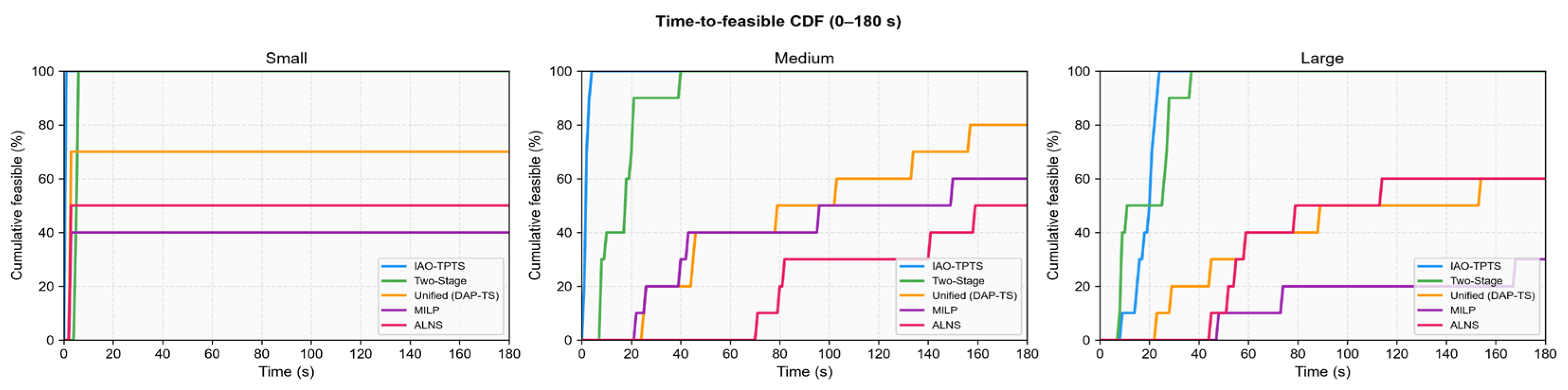
As shown in Figure 10, IAO-TPTS attains a 100% feasibility rate within the 180 s budget on all three scales. On Small instances, the median time to the first feasible solution is 0.069 s, substantially lower than 5.231 s for Two-Stage. On Medium instances, Unified (DAP-TS) and MILP achieve 80.0% and 60.0% feasibility, respectively, whereas IAO-TPTS remains at 100%; on Large instances, MILP drops to 30.0%, while IAO-TPTS again reaches 100%.

Figure 10. CDF of time to first feasible solution (0–180 s).

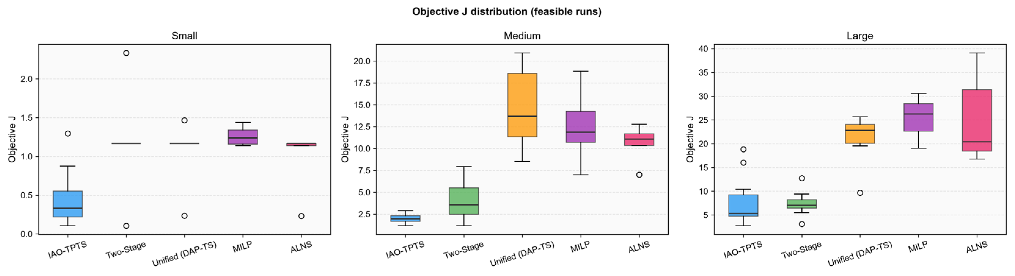
These MILP figures are not global optima. Under the same 180 s limit, MILP feasibility is only 40.0% (Small), 60.0% (Medium), and 30.0% (Large), and the mean J on feasible MILP runs is 1.26, 12.50, and 25.30, versus 0.47, 2.02, and 7.85 for IAO-TPTS. A proven optimum cannot be both substantially more costly than a feasible heuristic on the same instance family and missing on a large fraction of Small and Large instances. The MILP row is therefore a time-capped incumbent, or infeasible if none was found. The earlier wording that “MILP finds the optimal solution” referred to the unlimited-time, zero-gap case and does not apply to Table 6. IAO-TPTS is compared with this time-limited MILP baseline, which is the relevant competitor for execution-phase CD&R.

Table 6. Comparison summary.

Scale	Method	Feas. (%)	Mean J	Median Time (s)
Small	IAO-TPTS	100.0	0.469	0.069
Small	Two-Stage	100.0	1.1772	5.231
Small	Unified (DAP-TS)	70.0	1.0765	2.666
Small	MILP	40.0	1.2629	2.768
Small	ALNS	50.0	0.9734	2.636
Medium	IAO-TPTS	100.0	2.0165	1.514
Medium	Two-Stage	100.0	4.0298	17.428
Medium	Unified (DAP-TS)	80.0	14.5998	61.741
Medium	MILP	60.0	12.4951	40.685
Medium	ALNS	50.0	10.5728	81.925
Large	IAO-TPTS	100.0	7.8527	19.67
Large	Two-Stage	100.0	7.3807	18.105
Large	Unified (DAP-TS)	60.0	20.7787	51.391
Large	MILP	30.0	25.3009	73.341
Large	ALNS	60.0	24.9105	56.361

Note: MILP entries are the best incumbent found within 180 s, not proven global optima. Mean J is computed over feasible runs only.

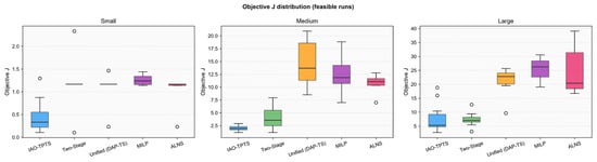
Figure 11 reports the objective value J on feasible runs. IAO-TPTS yields the lowest or near-lowest mean J on Small and Medium scales. On Large instances, its mean J is 7.8527, slightly higher than 7.3807 for Two-Stage but lower than Unified, MILP, and ALNS.

Figure 11. Objective J on feasible runs.

Overall, IAO-TPTS outperforms Unified, MILP, and ALNS in both feasibility and solution quality, and Two-Stage in computational efficiency on Small and Medium scales. On Large instances, Two-Stage attains a marginally lower mean J, yet IAO-TPTS offers stronger feasibility robustness under increased problem scale.

5.5. Sensitivity Analysis

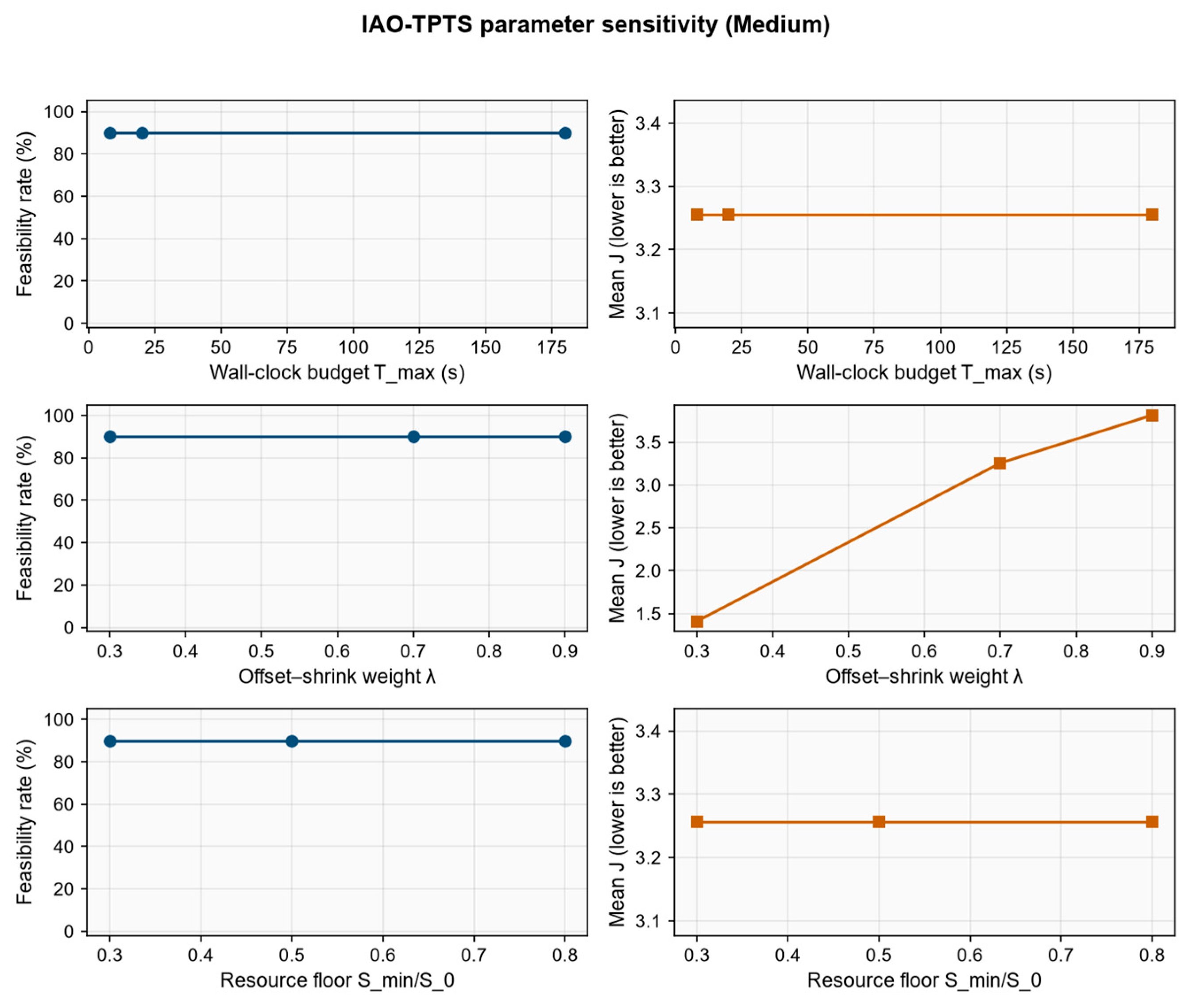
A one-factor-at-a-time sensitivity study is conducted on Medium-scale instances with the full IAO-TPTS configuration (V0). Ten seeds follow the same generation protocol as Section 5.3. Each factor is varied while the remaining parameters stay at Section 5.1 defaults (wall-clock budget T_max = 180 s, offset–shrink weight λ = 0.7, resource-preservation ratio S_min/S_0 = 0.5). Operational horizontal and vertical separation are not swept: they are occupancy-construction rules (Section 2.3), not online decision variables. The reported metrics are the feasibility rate, mean J on feasible runs, mean wall-clock time, the T2 modification rate z^0, and mean shrinkage. Table 7 and Figure 12 summarize the ninety runs (ten seeds × three factors × three levels).

Table 7. One-at-a-time sensitivity of IAO-TPTS (V0) on Medium instances (n = 10 seeds).

Factor	Level	Feas. (%)	Mean J	Mean Time (s)	T2 Mod. (%)	Mean Shrink
T_max (s)	8	90.0	3.26	2.28	0.0	0.4
	20	90.0	3.26	3.81	0.0	0.4
	180 *	90.0	3.26	19.82	0.0	0.4
λ (offset vs. shrink)	0.3	90.0	1.41	19.82	0.0	0.0
	0.7 *	90.0	3.26	19.83	0.0	0.4
	0.9	90.0	3.81	2.75	0.0	3.4
S_min/S_0	0.3	90.0	3.26	19.84	0.0	0.4
	0.5 *	90.0	3.26	19.83	0.0	0.4
	0.8	90.0	3.26	19.83	0.0	0.4

* Default value used in Section 5.1, Section 5.2, Section 5.3 and Section 5.4. Feasibility is 9/10: one Medium seed is infeasible under every treatment.

Figure 12. Sensitivity of IAO-TPTS (V0) on Medium instances.

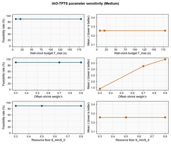
The wall-clock budget T_max ∈ {8,20,180} s does not change the certified set: feasibility remains 90.0% and mean J remains 3.26 at every level. The single infeasible seed is the same instance under all three budgets, so the shortfall is scenario hardness rather than an insufficient time cap. On the nine feasible seeds, J is identical across the three budgets, and the mean runtime remains about 2 s. The rise in the all-seed mean time from 2.28 s to 19.82 s in Table 7 is produced by the one infeasible seed, which exhausts the allotted budget (about 7.7 s, 19.1 s, and 179 s). Extra time therefore does not buy additional feasible solutions or a lower J; T2 remains locked (z⁰ = 0). The default 180 s budget of Section 5.1 therefore lies on a performance plateau for Medium instances: an 8 s cap already recovers the same feasible solutions.

The offset–shrink weight λ is the only factor that moves J. Increasing the relative penalty on shrinkage (λ = 0.3) yields mean J = 1.41 with zero shrinkage. The default λ = 0.7 gives mean J = 3.26 and a mean shrinkage of 0.4 grid units. Preferring offset cost (λ = 0.9) raises mean J to 3.81 and mean shrinkage to 3.4. Feasibility stays at 90.0%, and z⁰ remains 0, so λ reshapes the T1 cost mix without relaxing the lexicographic baseline lock. The default λ = 0.7 is therefore retained as a balanced setting rather than as a J-minimizing extreme.

The resource-preservation ratio S_min/S₀ ∈ {0.3,0.5,0.8} coincides with the default row on every metric. With default λ, the accepted solutions barely shrink, so tightening or relaxing the floor does not bind. This supports keeping the resource bounds of Table 3 as input limits rather than as independently tuned online parameters.

Across all ninety runs, the T2 modification rate is 0%. Parameter sensitivity therefore affects ad hoc cost and, when time remains, polish duration; it does not alter Stage-1/Stage-2 baseline protection.

5.6. Scalability and Case Study

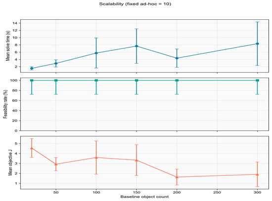
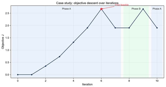
Part (1): scalability with 10 fixed ad hoc airspaces and baseline count 20–300. Part (2): a Medium case tracing J over iterations and per-airspace adjustments. This quantitative case differs from the visualization instance in Section 5.2.

Figure 13 reports scalability with ten fixed ad hoc airspaces and baseline counts increasing from 20 to 300. IAO-TPTS maintains a 100% feasibility rate across all 60 runs, while the mean solve time increases from approximately 1.5 s to 8.3 s, exhibiting sub-linear growth as the baseline scale expands. This indicates that the incremental detection and localized search remain computationally tractable at larger instance sizes.

Figure 13. Scalability (fixed ad hoc = 10).

Figure 14 traces the objective value J over iterations for a representative Medium-scale case. During Phase A, J increases temporarily as the search explores adjustment combinations; the first certified feasible solution appears at iteration 6 (J = 2.67), after which J converges to approximately 1.90. Phase B subsequently performs local refinement on this incumbent. The pre-feasibility increase in J reflects exploration cost during search, rather than algorithmic divergence.

Figure 14. Case study: objective J vs. iteration.

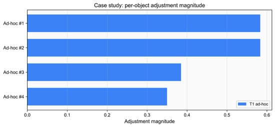
Figure 15 summarizes per-airspace adjustment magnitudes. All four T1 ad hoc airspaces are displaced, with magnitudes ranging from 0.35 to 0.58, whereas all T2 baseline airspaces remain unchanged (adjustment magnitude = 0). This outcome is consistent with the tiered protection policy and the Stage-1 priority rule that favors ad hoc adjustment over baseline modification.

Figure 15. Case study: per-airspace adjustment magnitudes.

5.7. Summary

Four experimental groups validate IAO-TPTS. Visualization shows combined horizontal, altitude, and temporal resolution on GeoSOT. Ablation confirms Phase A for quality and Phase B for feasibility. Comparison shows best or near-best feasibility and J within 180 s. Scalability remains 100% feasible up to 300 baselines with second-scale runtime. Future work: larger real-track datasets and denser conflicts to test T2 protection and dual validation margins.

6. Conclusions

As air traffic density rises and ad hoc missions become more frequent, airspace management during the execution phase requires fast, reliable, and minimally disruptive conflict detection and resolution (CD&R). Pre-planned baseline plans must remain largely intact, while newly inserted airspace objects must be incorporated online without triggering global re-optimization. To address this challenge, this paper proposed a grid-based online optimization framework and instantiated it through the IAO-TPTS algorithm for ad hoc airspace insertion on GeoSOT adaptive grids.

Methodologically, the framework transforms four-dimensional conflict judgment into efficient grid-code matching and interval comparison. Incremental P_adhoc detection restricts online checks to candidate pairs involving ad hoc objects, reducing detection scale by over 99% relative to full pairwise screening (Table 4). Resolution is governed by a lexicographic two-stage policy: Stage 1 adjusts ad hoc objects only, preserving the baseline whenever feasible; Stage 2 permits limited coordination on a conflict-related local subset only when necessary. IAO-TPTS operationalizes this policy under a hard wall-clock budget via Phase A (DCDA-Lite) for fast ad hoc-only feasibilization and Phase B (Hybrid-ALNS) for tiered refinement, with dual validation to prevent secondary conflicts in neighboring airspace.

Experimental validation across visualization, ablation, comparison, scalability/case studies, and sensitivity analysis confirms the effectiveness of the proposed approach. Visualization on GeoSOT grids demonstrates that IAO-TPTS can combine horizontal shift, altitude separation, and grid refinement within a unified 4D resolution process while prioritizing ad hoc (T1) adjustments and protecting baseline (T2) objects. Ablation results show that Phase A is essential for solution quality: skipping it raises mean objective J from 1.95 to 4.07 and increases variance (std 1.13 to 2.53). When Phase A certifies a Stage-1 solution, Phase B polishes T1 objects only and keeps T2 locked (T2 modification rate 0%; Stage-1 pure rate 100%). When Phase A alone is insufficient, Phase B restores feasibility (93.3% to 96.7%); the modest rise in V0 mean J relative to V1 is consistent with additional, more difficult instances becoming certified. Compared with Two-Stage, Unified (DAP-TS), MILP, and ALNS, IAO-TPTS achieves 100% feasibility within 180 s on all tested scales, with median solve times as low as 0.069 s on Small instances and competitive or superior objective values. Scalability tests with 10 fixed ad hoc airspaces and baseline counts from 20 to 300 maintain 100% feasibility with sub-linear runtime growth (~1.5 s to ~8.3 s), indicating practical applicability to medium- and large-scale online scenarios. A one-at-a-time sensitivity study on Medium instances shows that the default 180 s budget and Table 3 resource floor lie on a plateau, whereas the offset–shrink weight λ changes J and shrinkage without unlocking T2 (z⁰ = 0).

In summary, this work makes three main contributions. First, an incremental grid-based conflict detection scheme tailored to ad hoc insertion avoids redundant global checks and supports real-time online operation. Second, a two-stage priority-adjustment and local-coordination strategy protects the pre-planned baseline while limiting disruption to conflict-related neighborhoods. Third, IAO-TPTS enhances online adaptability of meta-heuristic search by constraining operations to localized grid adjustments and tiered object sets, thereby improving both speed and stability under strict time budgets.

Several limitations remain. The experiments rely on synthetic random scenarios rather than operational flight-track data; The numerical operational separation minima are operational rules used when the input occupancies are constructed, not decision variables of the optimization model. They are therefore not swept independently in the present experiments. A dedicated buffer-sensitivity study on live traffic is left to future work. Conflict density and geometry may differ in real airspace operations. Under Medium-density instances in which Stage-1 is typically certified, T2 objects remain unmodified ($z^0=0$) and V0 coincides with the no-T2 ablation, as required by the lexicographic policy. The benefit of unlocking T2 appears when Phase A cannot certify Stage-1 feasibility, and their benefits may emerge only in denser or more constrained environments. Furthermore, the current model assumes discrete grid occupancy and predefined operation primitives; integration with continuous trajectory management and human-in-the-loop approval workflows deserves further study.

Future work will pursue three directions: (1) validation on large-scale real track and mission data to assess engineering deployability; (2) stress testing under higher conflict density and tighter time/altitude windows to quantify the marginal value of tiered protection and dual validation; and (3) extension to multi-source dynamic demands, including UAV corridors and temporary restricted areas, with distributed implementation for operational airspace management systems. We expect the proposed grid-based online framework to serve as a practical foundation for safe and efficient ad hoc airspace insertion during the execution phase.

References

- Ribeiro, M.; Ellerbroek, J.; Hoekstra, J. Review of Conflict Resolution Methods for Manned and Unmanned Aviation. Aerospace 2020, 7, 79. [Google Scholar] [CrossRef] [Scilit]
- Zeng, W.; Chu, X.; Xu, Z.; Liu, Y.; Quan, Z. Aircraft 4D Trajectory Prediction in Civil Aviation: A Review. Aerospace 2022, 9, 91. [Google Scholar] [CrossRef] [Scilit]
- Tang, H.; Robinson, J.E.; Denery, D.G. Tactical Conflict Detection in Terminal Airspace. J. Guid. Control Dyn. 2011, 34, 403–413. [Google Scholar] [CrossRef] [Scilit]
- Ruiz, S.; Piera, M.A.; Nosedal, J.; Ranieri, A. Strategic De-Confliction in the Presence of a Large Number of 4D Trajectories Using a Causal Modeling Approach. Transp. Res. Part C Emerg. Technol. 2014, 39, 129–147. [Google Scholar] [CrossRef] [Scilit]
- Martinez, S.A.; Chatterji, G.B.; Sun, D.; Bayen, A.M. A Weighted-Graph Approach for Dynamic Airspace Configuration. In Proceedings of the AIAA Guidance, Navigation and Control Conference and Exhibit, Hilton Head, SC, USA, 20–23 August 2007. [Google Scholar]
- Yang, X.; Wei, P. Scalable Multi-Agent Computational Guidance with Separation Assurance for Autonomous Urban Air Mobility. J. Guid. Control Dyn. 2020, 43, 1473–1486. [Google Scholar] [CrossRef] [Scilit]
- Sun, G.; Qu, T.; Han, B.; Sun, H.; Zhang, Q. Research on Airspace Grid Modeling Based on GeoSOT Global Subdivision Model. In Proceedings of the 2021 IEEE 3rd International Conference on Civil Aviation Safety and Information Technology (ICCASIT), Changsha, China, 20–22 October 2021; pp. 501–505. [Google Scholar]
- Deng, C.; Cheng, C.; Qu, T.; Li, S.; Chen, B. A Method for Managing ADS-B Data Based on a 4D Airspace-Temporal Grid (GeoSOT-AS). Aerospace 2023, 10, 217. [Google Scholar] [CrossRef] [Scilit]
- Shu, P.; Zheng, Y.; Shi, H.; Liu, S.; Sun, H.; Zhou, X. Three Dimensional Grid Model of Airspace Resources Based on Beidou Grid Code. In Proceedings of the 2021 IEEE 3rd International Conference on Civil Aviation Safety and Information Technology (ICCASIT), Changsha, China, 20–22 October 2021; pp. 380–383. [Google Scholar]
- Acevedo, J.J.; Castaño, Á.R.; Andrade-Pineda, J.L.; Ollero, A. A 4D Grid Based Approach for Efficient Conflict Detection in Large-Scale Multi-UAV Scenarios. In Proceedings of the 2019 International Workshop on Research, Education and Development on Unmanned Aerial Systems (RED-UAS), Cranfield, UK, 25–27 November 2019; pp. 18–23. [Google Scholar]
- Miao, S.; Cheng, C.; Zhai, W.; Ren, F.; Zhang, B.; Li, S.; Zhang, J.; Zhang, H. A Low-Altitude Flight Conflict Detection Algorithm Based on a Multilevel Grid Spatiotemporal Index. ISPRS Int. J. Geo-Inf. 2019, 8, 289. [Google Scholar] [CrossRef] [Scilit]
- Zhai, W.; Han, B.; Li, D.; Duan, J.; Cheng, C. A Low-Altitude Public Air Route Network for UAV Management Constructed by Global Subdivision Grids. PLoS ONE 2021, 16, e0249680. [Google Scholar] [CrossRef] [Scilit] [PubMed]
- An, J.X.; Wang, W.X.; Liu, Z.; Zhang, J.Q. A Route Planning Method Based on the Airspace Divided by Grid Method. In Environmental Protection and Resource Utilization IV; Trans Tech Publications: Bäch, Switzerland, 2015; Volume 1073–1076, pp. 2381–2384. [Google Scholar]
- Pelegrín, M.; D’Ambrosio, C. Aircraft Deconfliction via Mathematical Programming: Review and Insights. Transp. Sci. 2022, 56, 118–140. [Google Scholar] [CrossRef] [Scilit]
- Liu, Y.; Zhou, Z.; Naqvi, W.; Chen, J. Strategic Deconfliction of Unmanned Aircraft Based on Hexagonal Tessellation and Integer Programming. J. Guid. Control Dyn. 2023, 46, 2362–2372. [Google Scholar] [CrossRef] [Scilit]
- Pan, W.; Qin, L.; He, Q.; Huang, Y. Three-Dimensional Flight Conflict Detection and Resolution Based on Particle Swarm Optimization. Aerospace 2023, 10, 740. [Google Scholar] [CrossRef] [Scilit]
- Zhou, Z.; Zhao, G.; Jiang, Y.; Wu, Y.; Yang, J.; Meng, L. Research on UAV Conflict Detection and Resolution Based on Tensor Operation and Improved Differential Evolution Algorithm. Aerospace 2024, 11, 1008. [Google Scholar] [CrossRef] [Scilit]
- Al-Nabhan, N.; Alturkestani, R.; Belghith, A.; AlAloula, N. A Conflict Resolution Approach for Multiple Unmanned Aerial Vehicles. Electronics 2025, 14, 2247. [Google Scholar] [CrossRef] [Scilit]
- Voigt, S. A Review and Ranking of Operators in Adaptive Large Neighborhood Search for Vehicle Routing Problems. Eur. J. Oper. Res. 2025, 322, 357–375. [Google Scholar] [CrossRef] [Scilit]
- Yang, W.; Tang, J.; He, R.; Chen, Y. A Medium-Term Conflict Detection and Resolution Method for Open Low-Altitude City Airspace Based on Temporally and Spatially Integrated Strategies. IEEE Trans. Control Syst. Technol. 2019, 28, 1817–1830. [Google Scholar] [CrossRef] [Scilit]
- Sun, B.; Yang, Y.; Zhang, S.; Li, J. Urban Economic Structure Impact on Passenger and Freight Efficiencies of Nine Airports in China: A Two-Stage Method. J. Nonlinear Convex Anal. 2026, 27, 987–999. [Google Scholar]
- Sun, B.; Xu, Z.; Ranjitkar, P.; Wei, M. DS-MGCSTNet: Multi-Graph Convolution Spatial-Temporal Network with Dynamic and Static Graph Fusion for Flight Delay Prediction. J. Air Transp. Manag. 2026, 136, 103047. [Google Scholar] [CrossRef] [Scilit]
Disclaimer/Publisher’s Note: The statements, opinions and data contained in all publications are solely those of the individual author(s) and contributor(s) and not of MDPI and/or the editor(s). MDPI and/or the editor(s) disclaim responsibility for any injury to people or property resulting from any ideas, methods, instructions or products referred to in the content. |
© 2026 by the authors. Licensee MDPI, Basel, Switzerland. This article is an open access article distributed under the terms and conditions of the Creative Commons Attribution (CC BY) license.