


Abstract
Prediction of turboshaft engine performance parameters is essential for engine health management, however, traditional physics-based models and shallow neural networks struggle to effectively model the complex nonlinear characteristics of time-series data. To overcome these limitations, a hybrid model integrating a Temporal Convolutional Network (TCN), an attention mechanism, and a Bidirectional Long Short-Term Memory (BiLSTM) network is proposed for predicting turboshaft engine performance parameters. Temporal convolution is employed to extract local temporal features, while the BiLSTM network is used to capture long-term bidirectional dependencies. An attention mechanism is further incorporated to assign greater weights to critical time steps. Simulation results show that the proposed model achieves higher prediction accuracy compared to standalone LSTM and TCN models. When applied to the performance prediction of turboshaft engines under different inlet air temperature conditions, the proposed framework consistently maintained the root mean square error values for training and testing between 0.05 and 0.09 across three key performance parameters, while effectively suppressing measurement noise. These results demonstrate that the model possesses excellent generalization performance and holds significant potential for practical engineering applications.
1. Introduction
As the primary power source of helicopters, accurate prediction of turboshaft engine performance parameters is critical to flight safety, operational reliability, and maintenance efficiency [1]. However, turboshaft engines are highly nonlinear thermodynamic systems whose complex physical mechanisms and strong interactions with environmental conditions make it difficult to establish high-fidelity physics-based models capable of accurately describing degradation behavior [2]. Consequently, data-driven machine learning methods have attracted increasing attention in aeroengine health management in recent years. Instead of relying on explicit modeling of degradation mechanisms, these approaches learn representative features directly from sensor measurements to establish data-driven predictive models, thereby enabling accurate forecasting of future engine performance trends [3].
Neural network-based methods have been extensively investigated for turboshaft engine performance prediction, Chen et al. applied BP neural networks to turboshaft engine parameter conversion, demonstrating the feasibility of shallow architectures for steady-state estimation [4]. Tan et al. employed Support Vector Machines (SVMs) to predict engine performance degradation indicators, achieving reasonable accuracy but with limited capability in handling long-term dependencies [5]. Cao and Wang further developed an adaptive SVM with a sliding time-window strategy for online prediction of engine performance parameters, yet the model’s reliance on manually selected features constrained its scalability [6]. Vladov and colleagues conducted a series of studies on helicopter turboshaft engine modeling using neural network approximations, demonstrating improved efficiency in parameter estimation [7,8,9]. To enhance prediction accuracy during transient operations, Dong et al. proposed a BSO-optimized Extreme Learning Machine (ELM) for turboshaft engine acceleration prediction, outperforming conventional BP and PSO-based ELM methods [10], while Song et al. successfully applied a K-means-ELM approach to engine power estimation [11]. For instance, Andrianantara et al. developed a neural network-based performance model for the CF34-8C5B1 turbofan engine, achieving high prediction accuracy for fan speed, core speed, turbine inlet temperature, net thrust, and fuel flow rate [12]. Despite these advances, such methods mainly rely on shallow network architectures and therefore exhibit limited capability in modeling the long-term temporal dependencies inherent in engine performance evolution.
To address the limitations of shallow learning methods, deep learning techniques have been increasingly adopted for aeroengine performance prediction. Wang et al. proposed a predictive maintenance scheduling framework for aircraft engines based on RUL prediction, demonstrating the practical value of deep learning in operational decision-making [13]. Dan et al. developed a Spike-TCN model with depthwise-separable convolution and attention mechanisms for efficient time-series prediction, showing that convolutional architectures can achieve competitive performance with lower computational costs [14]. Li et al. combined CNN, LSTM, and a self-attention mechanism (SAM) for turbofan engine RUL prediction, achieving improved accuracy through multi-scale feature extraction [15]. Dida et al. employed an Attention–LSTM neural network for aircraft engine RUL prediction, highlighting the effectiveness of attention mechanisms in focusing on critical degradation stages [16]. Yang et al. proposed an SDPA-BiLSTM model with an enhanced attention mechanism, further improving RUL prediction accuracy [17], while Zhu et al. developed a hybrid CNN-BiLSTM model with simulated annealing optimization for engine RUL prediction [18]. More recently, hybrid architectures integrating Temporal Convolutional Network (TCN), Bidirectional Long Short-Term Memory (BiLSTM) networks, and attention mechanisms have attracted considerable attention owing to their ability to simultaneously capture local temporal patterns and long-range dependencies. For example, Wang et al. proposed an interpretable TCN–EM–BiLSTM–Attention framework for remaining useful life prediction, achieving state-of-the-art performance on the C-MAPSS benchmark [19]. Similarly, CNN–LSTM–Attention architectures have also demonstrated improved prediction accuracy for aircraft engine remaining useful life estimation [20]. In addition, LSTM autoencoders combined with self-attention mechanisms have been successfully applied to anomaly detection in aircraft engine time-series data [21], while multiscale dilated fusion attention models effectively overcome the limitations of conventional CNNs and RNNs under complex operating conditions through parallel dilated convolutions and attention mechanisms [22].
Despite these advances, several challenges remain. Most existing studies have focused on turbofan engines rather than turboshaft engines, whose operating characteristics and mission profiles differ significantly. Moreover, existing research has primarily emphasized fault diagnosis and remaining useful life prediction, whereas relatively few studies have investigated multi-step prediction of turboshaft engine performance parameters. In addition, the robustness of deep learning models under varying environmental conditions, particularly under non-standard atmospheric conditions, has received limited attention. These limitations motivate the development of a more accurate and robust prediction framework for turboshaft engine performance prediction.
To address the aforementioned challenges, an attention-enhanced TCN–BiLSTM hybrid framework is proposed for the time-series prediction of turboshaft engine performance parameters. The TCN [23] is employed to extract local temporal features while expanding the receptive field to capture long-range temporal dependencies. A BiLSTM [24] network is incorporated to capture bidirectional temporal dependencies, while an attention mechanism [25] is introduced to adaptively weight informative hidden states, thereby emphasizing critical temporal features. By integrating these three components into a unified framework, the proposed model simultaneously captures local temporal patterns, global contextual information, and salient features from time-series data. In addition, a principal component analysis (PCA)-based feature selection scheme and a multi-scenario degradation data generation strategy are developed to provide representative input features and a comprehensive validation framework for model training and evaluation. Finally, two complementary prediction strategies, namely multivariate forecasting and univariate autoregressive forecasting, are investigated. Comparative experiments demonstrate the capability of the proposed framework to accurately track the evolution of turboshaft engine performance parameters under different information availability scenarios while confirming its potential for practical engineering applications. Although the individual components of the proposed architecture—the TCN, the BiLSTM, and the attention mechanism—are all well-established techniques in the existing literature, their integration into a unified framework for turbo-shaft engine performance prediction constitutes the core contribution of this study. The series-parallel topology specifically designed in this paper synergistically combines the advantages of local feature extraction and global bidirectional dependency modeling, enhanced by adaptive feature weighting. Through the organic series connection of these three modules, it achieves comprehensive extraction of local, global, and key features from time-series data. At the same time, this paper proposes a feature selection scheme based on principal component analysis and a multi-scenario degraded data generation strategy, providing high-quality input features and a benchmark validation environment for model training. Through comparative experiments between two approaches—multi-parameter mapping prediction and single-parameter autoregressive prediction—the paper systematically verifies the model’s ability to track trends in the performance parameters of turboshaft engines under different information conditions, as well as its engineering applicability.
The remainder of this paper is organized as follows. Section 2 introduces the theoretical foundations and the proposed TCN–BiLSTM–Attention hybrid model, followed by its validation using chaotic time-series data. Section 3 presents the application of the proposed model to turboshaft engine performance prediction, including the design of the prediction framework and the corresponding simulation-based validation. Finally, the conclusions are summarized in Section 4.
2. The TCN-BiLSTM Algorithm Based on Attention Mechanisms
2.1. Recurrent Neural Network and Its Variants
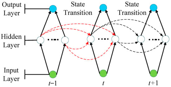
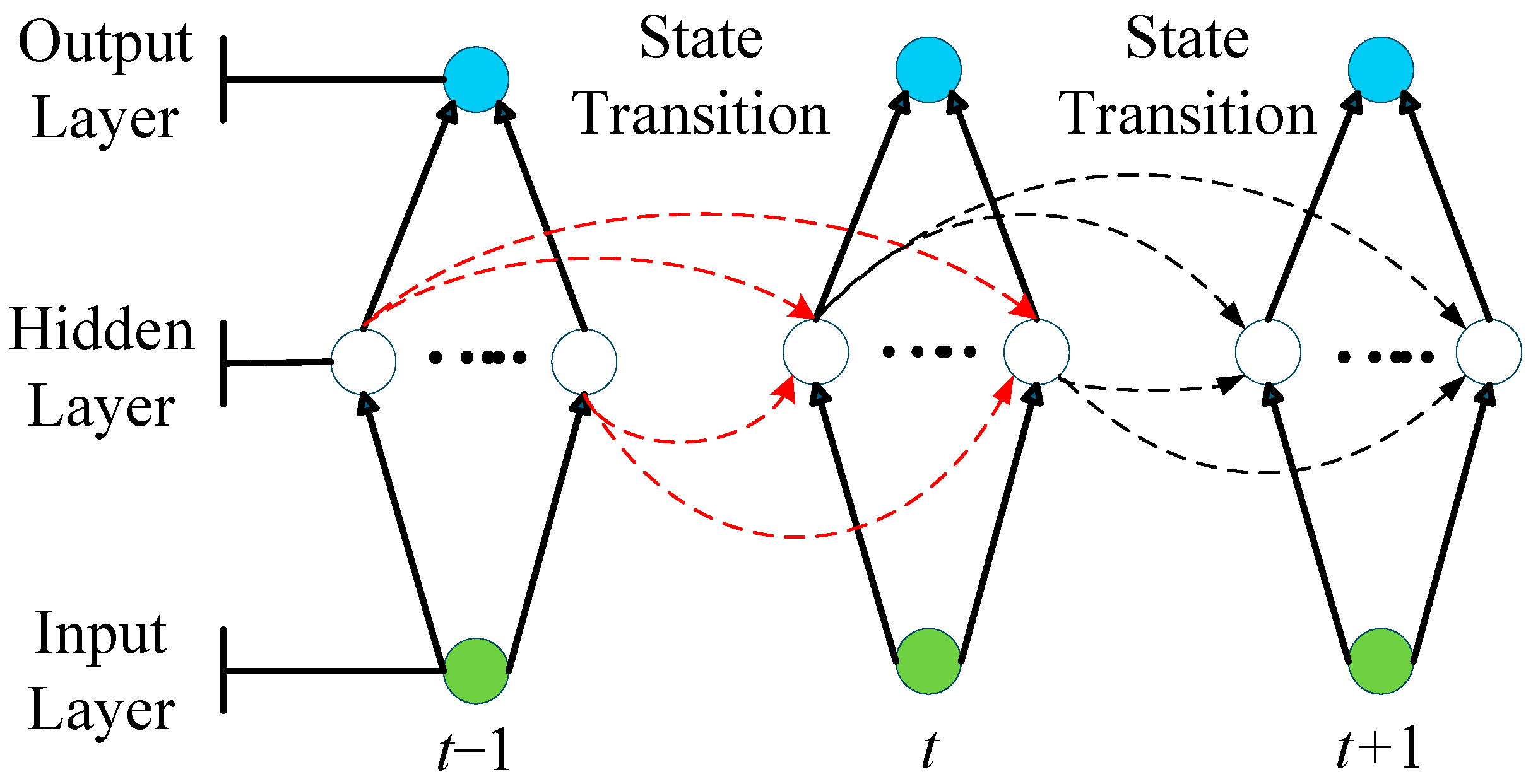
The core feature of recurrent neural networks (RNNs) lies in their ability to model dynamic changes in time-series data, thereby effectively handling the temporal dependencies that exist between samples. Structurally, an RNN incorporates the output of the hidden layer from the previous time step as a state into the input space of the next time step, as shown in Figure 1.
Figure 1.
Schematic diagram of an RNN network architecture.
Suppose the length of the time series to be processed is T, , and , represent the input vector, hidden-layer state vector, and output vector at time step t, respectively; n, d, and m represent the input feature dimension, the number of hidden-layer neurons, and the output vector dimension, respectively. Then, the hidden-layer state of the RNN is determined jointly by the input at the current time step and the state at the previous time step, that is,
where is the weight matrix from the input layer to the hidden layer, is the weight matrix from the hidden layer to its own recurrent connection, is the bias vector of the hidden layer, and is the activation function of the hidden layer.
Since already contains all historical information, the output at the current time step is determined solely by the hidden state at that time step. However, when traditional RNN are trained using the backpropagation through time (BPTT) algorithm, the chain multiplication of gradients along the time axis can easily lead to vanishing or exploding gradients, making it difficult for them to capture long-term dependencies.
To address the vanishing gradient problem in traditional RNN, researchers have proposed various RNN variants, the most common of which is the Long Short-Term Memory (LSTM) network. The core improvement of LSTM is the replacement of the single hidden state in traditional RNNs with both a hidden state and a cell state , along with the introduction of three gate units: the input gate, the forget gate, and the output gate. By controlling the activation and deactivation of these gate units, the update of the cell state and the propagation of information are regulated, thereby effectively mitigating the gradient vanishing problem and enabling stable modeling of long sequences.
The forget gate is used to determine which information from the cell’s state at the previous time step should be discarded, and it is calculated as follows:
where is the logistic function. The is the Input Gate, which determines which information from the candidate states at the current time step should be added to the new cell state , and is calculated as follows:
where is the tanh function, is the candidate cell state at the current time step, and is the state update amount.
The output gate determines which information from the current cell state should be output to the hidden state. It is calculated as follows:
Furthermore, the bidirectional long short-term memory (BiLSTM) network adds a parallel, backward-processing LSTM layer to the standard LSTM, enabling the hidden state at each time step to simultaneously integrate both forward and backward contextual information. This allows for a more comprehensive capture of bidirectional long-range dependencies in sequences, making it particularly suitable for scenarios involving mutual constraints between preceding and subsequent states in the performance evolution of turboshaft engines.
2.2. Temporal Convolutional Network
Temporal Convolutional Network (TCN) is a variant of convolutional networks designed specifically for time-series data. Its core advantage lies in its ability to process long sequences by leveraging the parallel computing capabilities of convolutions, while avoiding the gradient backpropagation issues associated with RNN. Its core architecture and key mechanisms primarily include causal convolution, dilated convolution, and residual connections, which are described below.
Causal convolution ensures that the output at time t depends only on the inputs at time t and earlier times by zero-padding only the left side of the input sequence, thereby strictly satisfying the causality constraints of time series forecasting.
The basic principle of dilated convolution is to introduce a dilation factor between the elements of the convolution kernel, allowing the kernel to cover a wider time span while maintaining its original size. For a one-dimensional sequence input and a filter , the dilated convolution operation F on sequence element s is defined as:
where d is the dilation factor, and k is the filter size. accounts for the past direction; thus, it can be seen that the essence of dilation is to introduce a fixed spacing between adjacent taps of the convolution kernel. Therefore, by incrementally increasing d layer by layer, the TCN’s receptive field can grow exponentially (i.e., in layer i, ), allowing an extremely long effective history window to be covered with just a small number of layers.
To mitigate the vanishing gradient problem in deep network training, TCN draws on the design philosophy of ResNet by directly concatenating the input to the output across layers in the residual blocks, effectively alleviating the vanishing gradient problem in deep network training and improving model stability.
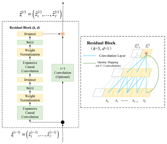
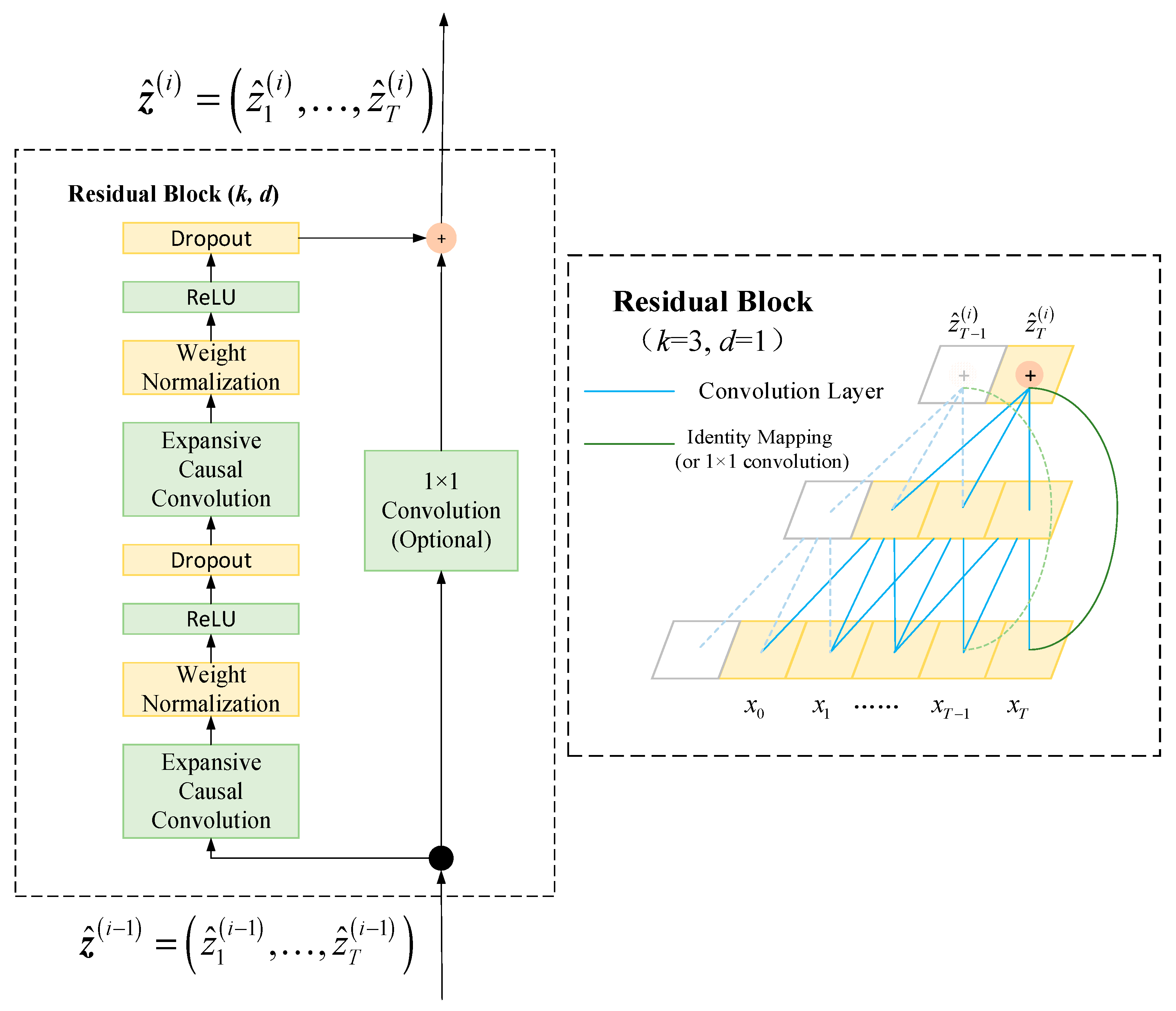
The residual blocks used in the standard TCN algorithm are shown in Figure 2 Each residual block contains two layers of expanded causal convolutions and a nonlinear activation function [26], and the weights of the convolutional filters are normalized [27]. Furthermore, a spatial dropout [28] is added after each layer of dilated convolutions to achieve regularization; specifically, the entire channel is set to zero at each training step.
Figure 2.
TCN Residual Block.
In summary, through the aforementioned design, TCN combines the advantages of efficient parallel training, flexible control of receptive fields, and stable gradient propagation; however, when relying solely on convolutional operations, its ability to model bidirectional temporal interactions remains weaker than that of BiLSTM. Therefore, combining the standard TCN algorithm with modules such as attention mechanisms and transformers could be considered to further improve performance.
2.3. Attention Mechanism
The core idea of the attention mechanism is to allow the model to dynamically assign different weights to information at different positions when processing sequential data, focusing on the parts most relevant to the current decision. Introducing attention mechanisms into deep learning allows the model to automatically identify which parts of the data are more critical. The mathematical expression for the attention mechanism is:
where Q, K, and V represent the query, key, and value matrices, respectively, and denotes the dimension of the key matrix. The data in the query matrix represents the information the model focuses on; the data in the key matrix is used to calculate the similarity between these pieces of information—that is, the attention scores; and the data in the value matrix is used to compute the final output based on these similarities. To prevent data from “exploding” due to an excessively large key dimension or “vanishing” due to an excessively small one during computation, these scores are typically scaled by dividing them by the square root of the key dimension. They are then converted into a weight distribution via the softmax function, and finally, these weights are multiplied by the value matrix to obtain the final attention vector output.
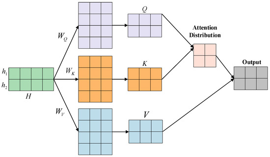
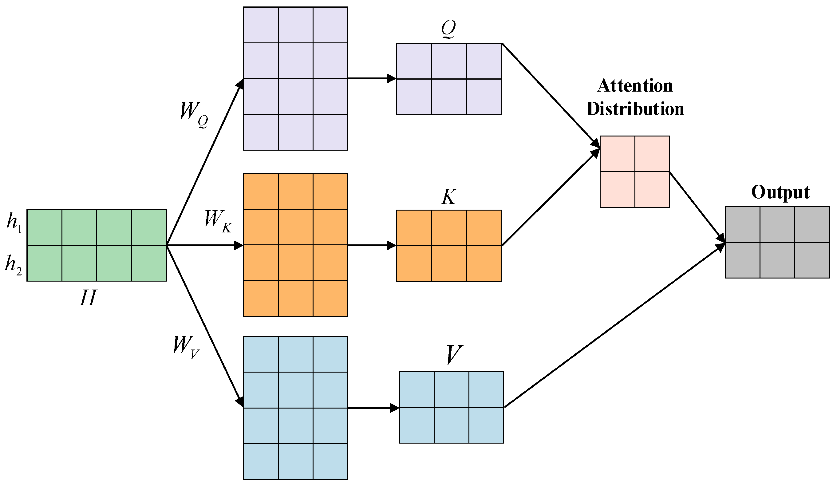
The attention mechanism adaptively allocates relevant weights across the entire sequence through the Q-K-V combination, overcoming the limitations of the restricted receptive field in convolutional networks and the gradual propagation of dependencies in recurrent networks. Its principle is illustrated in Figure 3.
Figure 3.
Principles of Attention Mechanisms.
2.4. Design of a TCN-BiLSTM Network Based on Attention Mechanisms
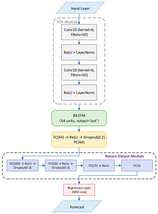
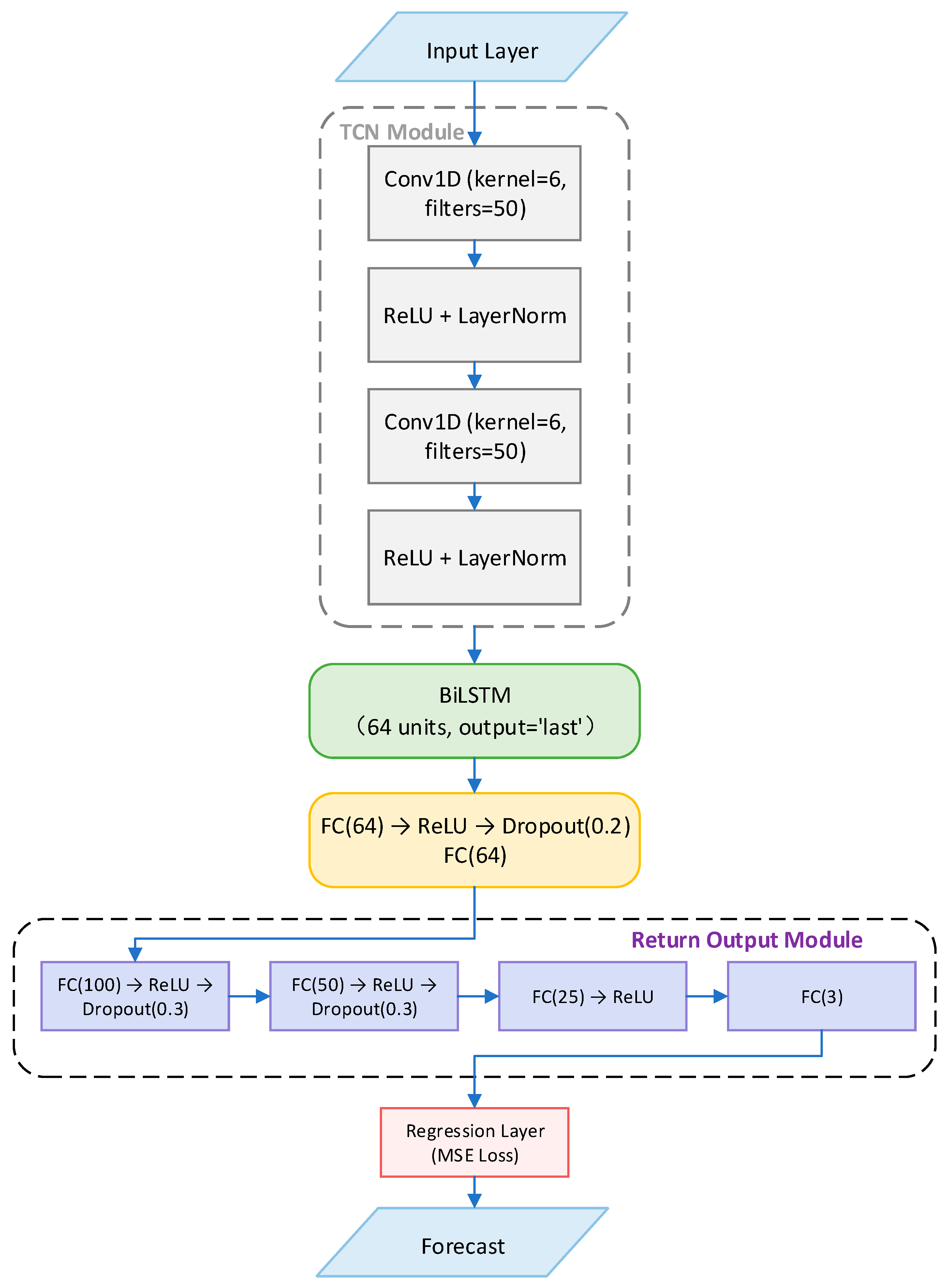
Having previously discussed the basic principles and characteristics of BiLSTM, TCN, and attention mechanisms, this section will further explain how to combine these three modules in a series-parallel configuration to construct a network model for time series forecasting. In this section, we design an attention-based TCN-BiLSTM network, whose topological structure is shown in Figure 4. In this architecture, the TCN module is responsible for extracting short-term local dependencies within the sequence, the BiLSTM module captures bidirectional long-term temporal features, and the attention mechanism adaptively weights and enhances these features. Finally, the regression output layer maps these features to multi-step forecast values.
Figure 4.
TCN-BiLSTM Network Architecture Based on Attention Mechanism.
The model’s input is a three-dimensional tensor constructed from a sliding window. Suppose the original dataset contains M time steps, with each step comprising D external input variables and the target variable y. To enhance the model’s autoregressive capability, in addition to the external variables at the current time step, the target variable values from the past H time steps are also used as additional features. Therefore, the effective feature dimension at each time step is . Next, a sliding window of length N1 is used to extract consecutive a continuous sequence along the time axis, forming the sample set , where and the corresponding output represent the target variable values for the next N2 time steps. All samples are randomly divided into training and testing sets according to a given ratio.
The network consists of an input layer, a TCN module, a BiLSTM module, and an attention module. The original input sequence first enters the TCN module, which is composed of a stack of multi-layer one-dimensional convolutional layers, each followed by a nonlinear activation function and a normalization layer. The TCN module’s output retains the sliding window length, with each time step represented by convolutional features; The sequence features output by the TCN are fed directly into the BiLSTM layer. The BiLSTM comprises two independent LSTM units—one forward and one backward—with the output mode configured to retain only the hidden state of the last time step. After bidirectional processing, the BiLSTM outputs a feature vector of fixed length that integrates long-term dependencies from both the forward and backward directions of the sequence. This feature vector is then fed into the attention module. This module consists of two fully connected layers, interspersed with activation functions and Dropout layers. The attention module outputs an enhanced feature vector with the same dimension as the input, achieving adaptive nonlinear transformation and weight allocation for the original features; The vector enhanced by the attention mechanism then passes sequentially through multiple fully connected layers, each followed by a corresponding activation function and a Dropout layer. Finally, it is mapped through the output layer to a prediction vector with the same dimension as the prediction step. The model as a whole employs a regression layer and uses mean squared error as the loss function.
Training was performed using the Adam optimizer, with appropriate learning rates, batch sizes, and maximum iteration counts set. To prevent overfitting, Dropout layers were introduced at multiple points in the network. Additionally, a normalization layer was used in the TCN module to accelerate convergence, and a progressive dimension reduction structure was adopted in the output module to reduce the number of parameters. The validation strategy was as follows: after each training round, the loss was calculated on the validation set, and the model with the lowest validation loss was saved as the final model.
2.5. Algorithm Verification
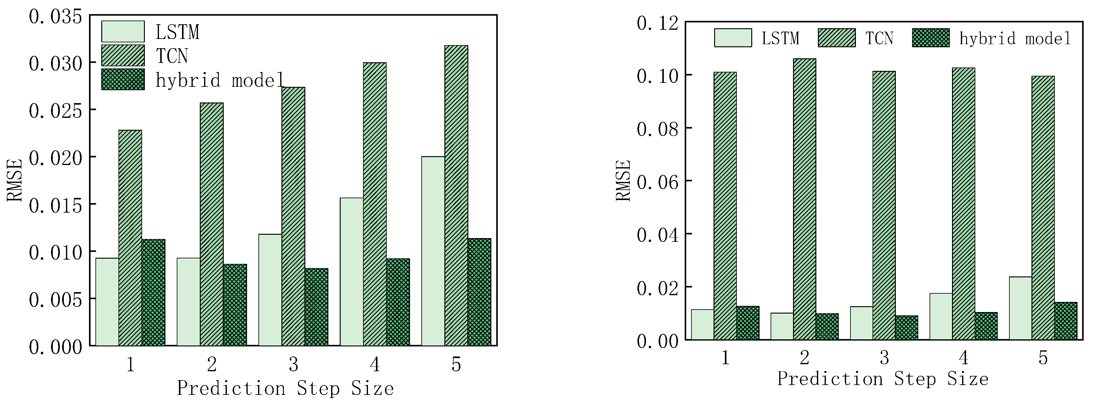
To validate the effectiveness of the TCN–BiLSTM–Attention integrated network proposed in this paper, it was applied to multi-step forecasting of Mackey–Glass and Lorenz chaotic time series. Comparative schemes, including LSTM and TCN networks, were also set up. By comparing multi-step forecasting error metrics such as RMSE, MAE, and R2, the advantages of this model in forecasting tasks on general-purpose datasets were evaluated. The forecasting problem is described as follows: Given a univariate time series, a nonlinear mapping of the predictor is constructed such that it satisfies Equation (10), and the predicted output is then used as the input for the next step to drive the iterative computation of the predictor.
Based on an autocorrelation analysis of chaotic time series, and to strike a balance between capturing sufficient historical information and maintaining computational efficiency, the sliding window size in this paper is set to 10. The number of prediction steps is set to 5 to evaluate the model’s multi-step forecasting capability, as this value represents a practically meaningful medium-term forecasting horizon while ensuring computational feasibility. To strike a reasonable balance between model training and generalization performance evaluation, the training set ratio was set to 0.8. Additionally, following standard choices widely adopted in deep learning literature, the learning rate was set to 0.001 and the batch size to 32. Through grid searches of the ranges {16, 32, 64} for the number of TCN filters and {2, 3, 4, 5} for the convolution kernel size, respectively, the number of TCN filters (32) and convolution kernel size (4) that yielded the lowest validation error on the Mackey–Glass dataset were ultimately selected. To provide sufficient representational capacity while avoiding excessive computational overhead or overfitting, the hidden unit size for the LSTM/BiLSTM layers was set to 64. These network parameter settings are shown in Table 1, and the simulation results are presented in Table 2 and Figure 5.
Table 1.
Network Parameter Setting.
Table 2.
Comparison of Chaotic Time Series Forecasting Metrics.
Figure 5.
Comparison of RMSE in Multi-Step Forecasting of Chaotic Time Series.
To comprehensively evaluate the prediction performance, three widely adopted metrics are employed: Root Mean Square Error (RMSE), Mean Absolute Error (MAE), and the Coefficient of Determination R2. RMSE measures the standard deviation of the prediction errors and is particularly sensitive to large deviations, making it suitable for penalizing significant prediction outliers. MAE provides a more interpretable measure of the average absolute prediction error. For both RMSE and MAE, smaller values indicate better prediction accuracy, as they reflect closer agreement between predicted and actual values. The R2 statistic quantifies the proportion of variance in the target variable that is explained by the model, with values ranging from 0 to 1. Larger R2 values (closer to 1) indicate superior model fit, whereas values approaching 0 suggest that the model fails to capture the underlying data variability. These three metrics are complementary: RMSE and MAE assess the magnitude of prediction errors, while R2 evaluates the overall explanatory power of the model. In the subsequent analysis, these metrics are jointly reported to provide a holistic assessment of the proposed framework’s predictive performance.
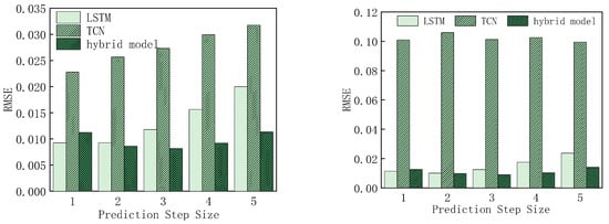
As shown in Table 2, on the Mackey–Glass dataset, the hybrid model’s RMSE is approximately 43.3% lower than that of the LSTM and approximately 64.3% lower than that of the TCN. Furthermore, its R2 value reaches 0.98, which is significantly higher than the LSTM’s 0.95 and the TCN’s 0.87; On the Lorenz-Y dataset, the hybrid model’s RMSE is approximately 40.5% lower than that of the LSTM and approximately 85.8% lower than that of the TCN, with an R2 as high as 0.99, whereas the TCN network’s R2 was only 0.68. This indicates that the pure TCN suffers from a severe decline in predictive capability on strongly non-stationary sequences such as Lorenz-Y, while the hybrid model effectively compensates for the TCN’s shortcomings in modeling long-term dependencies through bidirectional LSTMs and attention mechanisms. Further examination of the step-by-step RMSE bar chart in Figure 5 reveals that as the prediction step size increases, the hybrid model exhibits the most gradual rise in error. Although the LSTM network has a lower error for single-step predictions, its error increases linearly as the prediction step size grows. Notably, at the 5th step of the Lorenz-Y dataset, the TCN’s RMSE has already exceeded 0.09, while the hybrid model remains around 0.014, demonstrating that the hybrid model exhibits exceptional robustness in long-term forecasting.
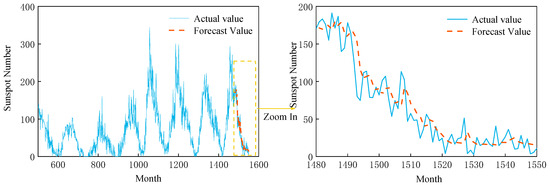
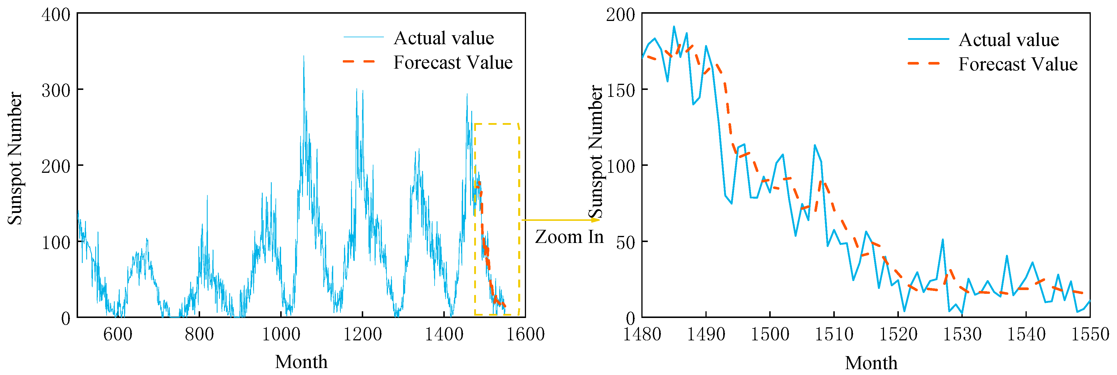
In addition, to validate the long-term forecasting capability of the TCN-BiLSTM hybrid model, it was applied to the forecasting problem using the sunspot dataset. The sunspot dataset, provided by the Swiss Observatory, is a classic univariate time series describing the periodic variations in solar activity. It is commonly used to evaluate the ability of time series forecasting models to capture nonlinear, nonstationary, and long-range dependent characteristics. In this section, 1000 data points from the dataset were selected as training samples to construct a single-step forecasting model that performs backward recursion to predict sunspot numbers for the next 70 months. Table 3 presents the multi-step extended forecast results for the three algorithms. The results indicate that the TCN-BiLSTM hybrid model achieves an RMSE of 19.58 on the test set, which is 9.5% lower than that of the LSTM model and 32.8% lower than that of the standalone TCN model. This represents a substantial improvement in prediction accuracy. Figure 6 compares the predicted values from the hybrid model with the observed values. It can be observed that the predicted curve from the TCN-BiLSTM hybrid model closely matches the observed curve across the entire forecasting horizon. The results indicate that the predicted values from the TCN-BiLSTM hybrid model closely match the observed curve and achieve the lowest RMSE.
Table 3.
Comparison of the Accuracy of Sunspot Number Forecasts.
Figure 6.
Sunspot Number Prediction Based on a TCN–BiLSTM–Attention Hybrid Model.
In summary, the TCN–BiLSTM–Attention hybrid model significantly outperforms both standalone LSTM and TCN models in terms of both prediction accuracy and long-term stability for multi-step forecasting of chaotic time series. This validates the superiority and generalizability of the proposed network architecture, making it suitable for time series modeling tasks such as the prediction of turboshaft engine performance parameters. For inference, the model produces predictions in milliseconds, making it suitable for near-real-time engine health monitoring applications.
3. TCN–BiLSTM-Based Turboshaft Engine Performance Prediction
During engine operation, understanding trends in its health status is a key prerequisite for predicting service life and making maintenance decisions. The task of performance parameter prediction involves converting multi-parameter measurement data into describable, extrapolable continuous trends; therefore, it can be viewed as a conditional time-series regression problem—that is, estimating target performance parameters over a subsequent period based on known historical multi-parameter sequences and environmental operating conditions. Based on this approach, this section employs the proposed TCN–BiLSTM–Attention hybrid model to perform modeling, learning, and trend prediction for the key performance parameters of turboshaft engines.
3.1. Component-Level Model of a Turboshaft Engine
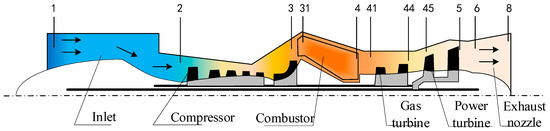
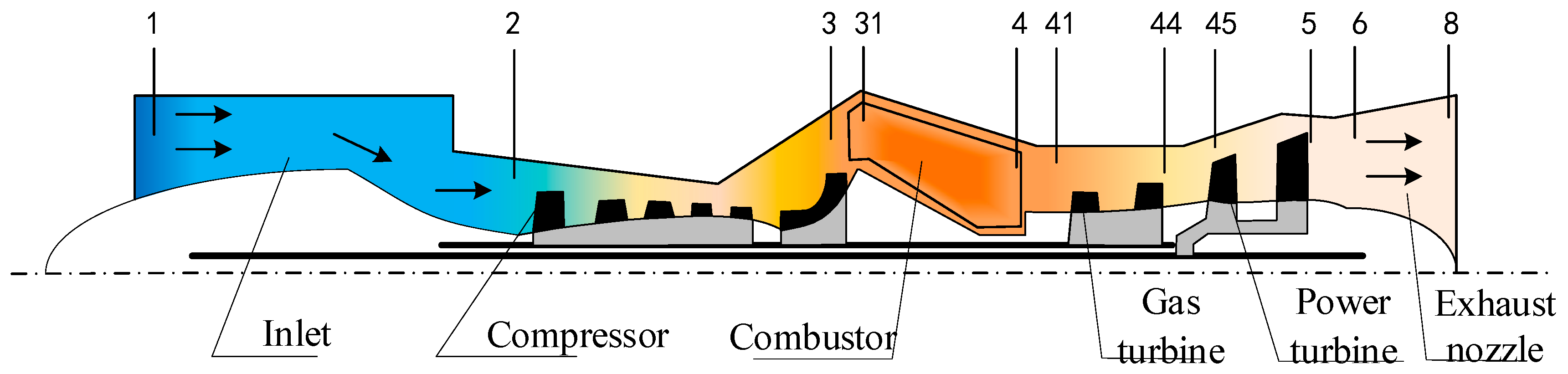
The subject of this study is a certain type of civil turboshaft engine, which consists of multiple components, including the inlet, compressor, combustor, gas turbine, power turbine, and exhaust nozzle. The component-level models are established based on the aerodynamic and thermodynamic principles of turboshaft engines; that is, models of each engine component are first constructed, and then combined into a complete engine model based on their common operating conditions. The resulting system of nonlinear algebraic equations is solved iteratively using the Newton–Raphson method to obtain the steady-state operating point for a given set of inputs. The airflow cross-sections of the turboshaft engine studied in this paper are shown in Figure 7.
Figure 7.
Structure of a Turboshaft Engine Component-Level Model.
The model is implemented in the MATLAB/Simulink R2020a environment, which provides a flexible platform for system-level simulation and integration with control system development. The steady-state and transient accuracies of this model have been validated against real ground-test data of a turboshaft engine in our previous work [29]. This validated model serves as the data generator for simulating the performance degradation processes under various health parameter and environmental conditions, thereby providing the synthetic dataset used for training and evaluating the proposed prediction framework.
3.2. A Strategy for Predicting the Performance Parameters of Turboshaft Engines
Principal Component Analysis (PCA) is an algorithm that simplifies data processing by reducing the dimensionality of features. It uses specific mathematical transformations to convert a large number of original variables into a smaller number of independent composite variables, while retaining most of the information contained in the original data. Because PCA can filter out some noise and interference while retaining the main features of the data, and because it has a simple structure and is easy to implement, it has been widely applied in practical engineering. This paper also uses Principal Component Analysis to analyze the performance parameters of turboshaft engines and, based on this, provides criteria for selecting reference sensor data, as detailed below.
Suppose the original data contains n samples and m indicators. These data can be used to construct a matrix a with n × m elements a. First, the data is standardized to calculate the mean and standard deviation for each column:
The standardized matrix element Aij is:
We then calculate the covariance matrix B of matrix A:
Then, calculate the eigenvalues and corresponding eigenvectors of matrix B to determine the principal component contribution rates and cumulative contribution rates.
Then, calculate the eigenvalues and corresponding eigenvectors of matrix B to determine the principal component contributing rates and cumulative contributing rates.
This paper employs principal component analysis to examine changes in measurement data from multiple sensors following the performance degradation of turboshaft engine components. After extracting deep-level features, measurement parameters that accurately reflect performance parameters are selected. The candidate measurement parameters include: Ng, W2, P3, T3, T45, EXT, PIC, P5 and T5. Based on the constructed component-level model, a steady-state point (H = 0, Ma = 0, Ng = 100%) is selected, and data are sampled every 25 flight cycles over a total simulation horizon of 500 flight cycles, yielding approximately 20 samples per degradation scenario. Six degradation scenarios are simulated, corresponding to different combinations of efficiency and flow capacity degradations in the three components, as detailed in Table 4.
Table 4.
Deviations in Measurement Parameters Corresponding to Changes in Health Parameters.
For each scenario, the generated dataset is split into training and testing sets with an 80/20 ratio, consistent with the experimental setup described in Section 2.5. Additionally, a validation set comprising 15% of the training data is reserved for model selection and early stopping during training. All data correspond to steady-state engine operation, as the prediction task focuses on tracking the long-term degradation trend rather than capturing transient dynamics. The total number of samples across all scenarios and environmental conditions is approximately 360 (6 scenarios × 3 temperatures × 20 samples), providing a sufficiently diverse dataset for training and evaluating the proposed framework.
Among the measurement parameters listed above, the parameters to be predicted are specific fuel consumption (SFC), gas turbine speed (Ng), and power turbine inlet temperature (T45). Therefore, the sensors Ng, EXT, and T45—which characterize these three performance parameters—must be selected. The remaining measurement parameters form a 5-row by 6-column matrix. Principal component analysis is performed on this matrix to reduce the number of sensors while minimizing multicollinearity. The results are shown in Table 5. Based on the comprehensive scores, the four measurement parameters P3, T3, P5 and T5 were ultimately selected.
Table 5.
Selection of Measurement Parameters.
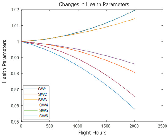
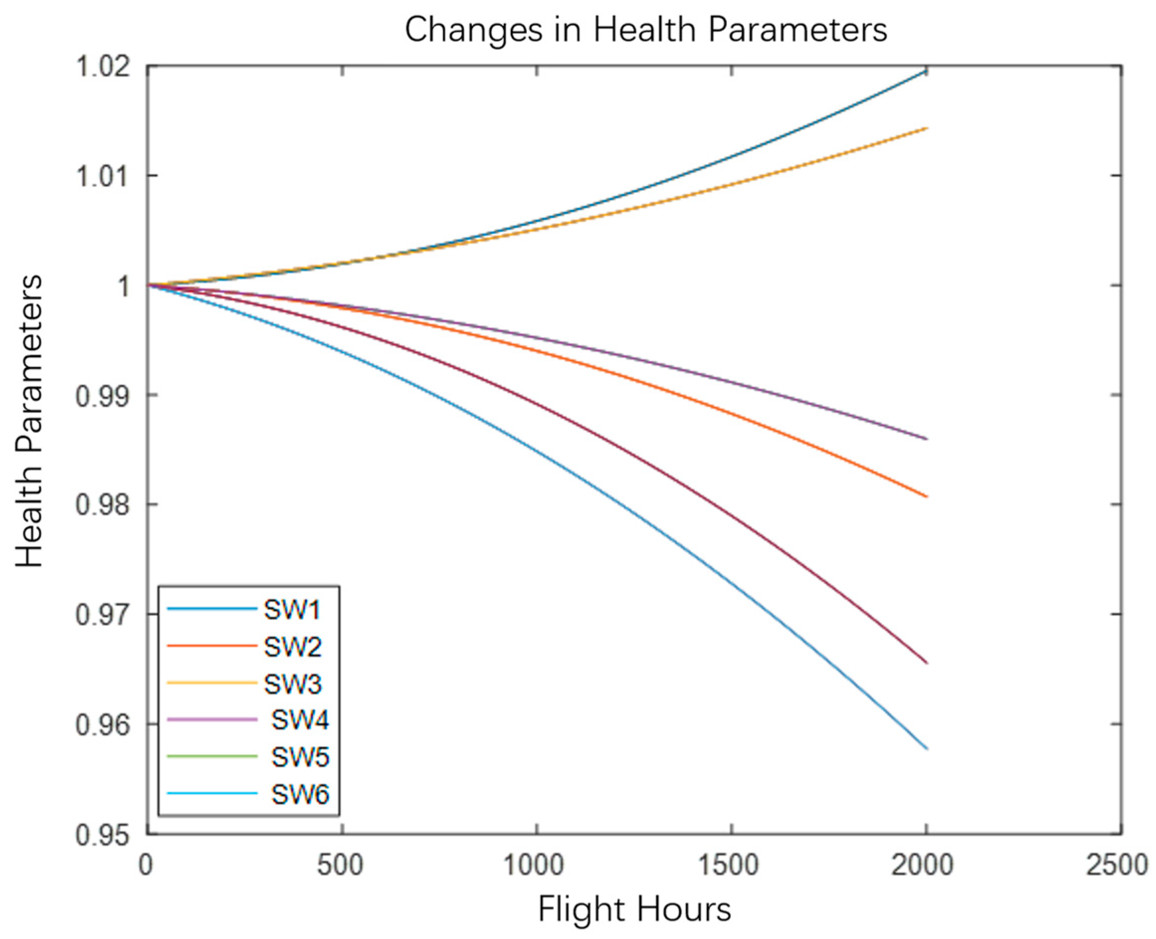
As engine operating hours increase, the degree of performance degradation varies among different components. Furthermore, due to differences in manufacturing processes between engines, their characteristics during the performance degradation process also differ. These differences can all be reflected by health parameters. The health parameters of a turboshaft engine’s gas path are primarily represented by changes in the efficiency and flow capacity of the compressor, gas turbine, and power turbine. Therefore, this section first simulates the performance degradation process of a turboshaft engine by adjusting these health parameters; with regard to engine degradation, based on NASA’s published data on turbofan engine degradation, the various rotor components of a turboshaft engine degrade according to the pattern shown in Figure 8 [30], where the flow coefficient and the efficiency coefficient are the health parameters for each rotor component [31], used to characterize the performance status of engine components; the subscript (i = 1, 2, 3) represents the three rotating components: the compressor, the gas turbine, and the power turbine, respectively.
Figure 8.
Patterns of Change in Health Parameters.
Based on the turboshaft engine model, degradation data were generated according to the trends in engine health parameters shown in Figure 8. Since engine performance degradation is a gradual process, data were collected every 25 flight cycles to form a degradation dataset. To enable early prediction of performance parameters, single-step predictions were performed two flight cycles in advance, establishing a correspondence between the current data and the data from the previous n time steps, thereby directly predicting the target values. Separate prediction models were established for the three performance parameters: specific fuel consumption (SFC), gas turbine rotational speed (Ng), and power turbine inlet temperature (T45).
SFC prediction model:
Ng prediction model:
T45 prediction model:
where n is the order of the time delay.
Furthermore, considering the different orders of magnitude of the measured parameters, the data must be normalized to improve the network’s training efficiency. This chapter adopts the maximum–minimum normalization method to normalize the sample data to the range [0, 1], as shown in Equation (17).
where and represent the original value and the normalized standard value, respectively, and and denote the maximum and minimum values of that parameter in the sample set.
In addition to establishing a mapping model between measurement parameters and performance parameters, the TCN–BiLSTM–Attention algorithm proposed in this chapter can also be directly used for autoregressive prediction of performance parameters. Specifically, it first performs a single-step prediction based on existing information, then uses the predicted value of the target parameter—as output by the network at the current time step—as the input to the network for the next time step, iterating step by step to obtain predicted values for the target parameter across the entire time series. This approach requires a relatively small amount of data; the network input consists solely of the target parameter itself, without involving other historical measurement data, and relies primarily on a sliding window. The mathematical expression for its prediction function is:
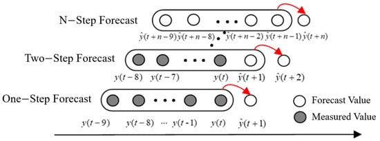
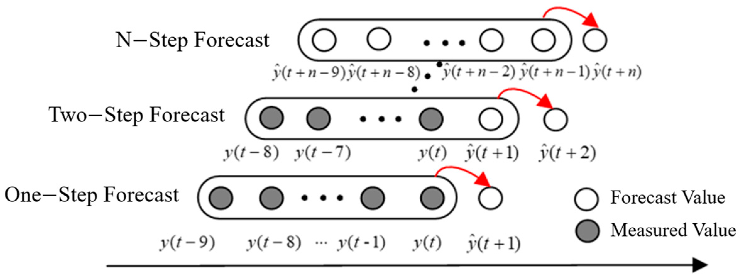
where y is the true target parameter, is the predicted target parameter, m is the sliding window length, and n is the prediction step size. When the sliding window length m = 10 and the prediction step size is n, the multi-step iterative prediction diagram is shown in Figure 9.
Figure 9.
Schematic Diagram of Multi-Step Iterative Forecasting.
During the training phase of a neural network, using existing sample data, a correspondence is established between the target parameter values at m consecutive time steps (i.e., the sliding window length) and the target parameter value at the next time step. During the testing phase, the target parameter value for the next time step is first predicted, then fed into the sliding window as the input for predicting , while the oldest data point in the window is removed to maintain the window length. Next, the value for the time step after that is predicted, and so on. Through this iterative process, predictions are obtained for the entire time series.
3.3. Simulation Verification and Analysis
A. Multivariate Forecasting
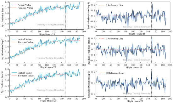
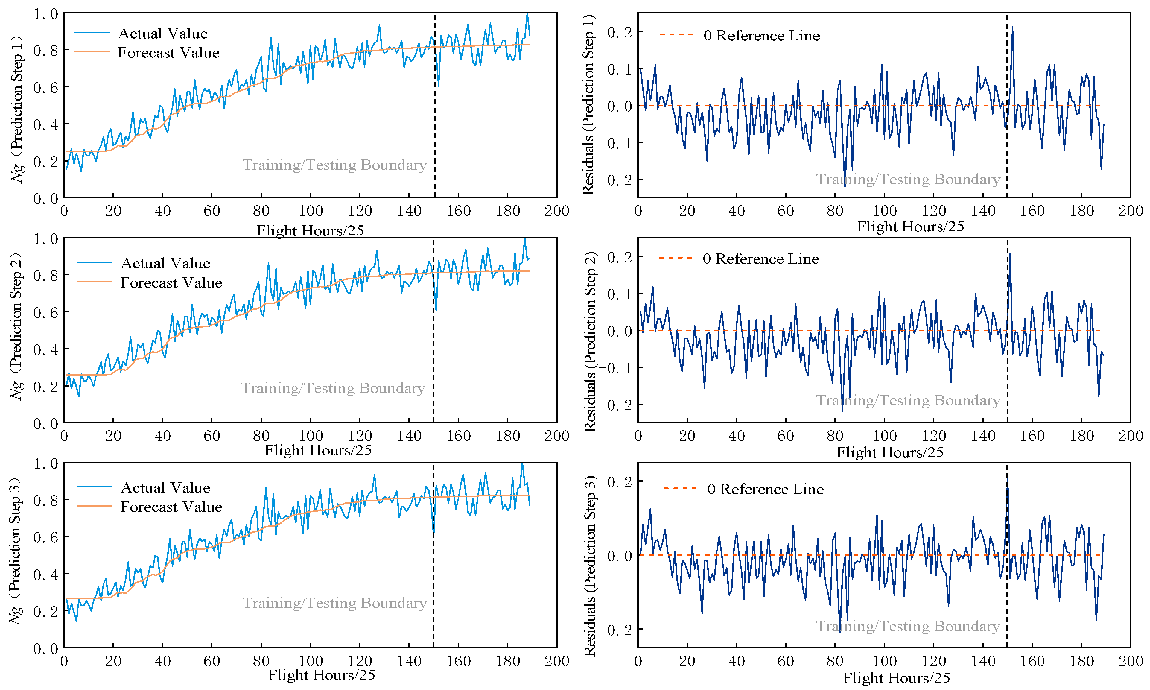
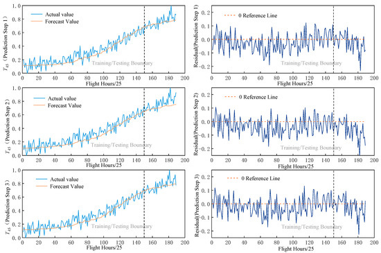
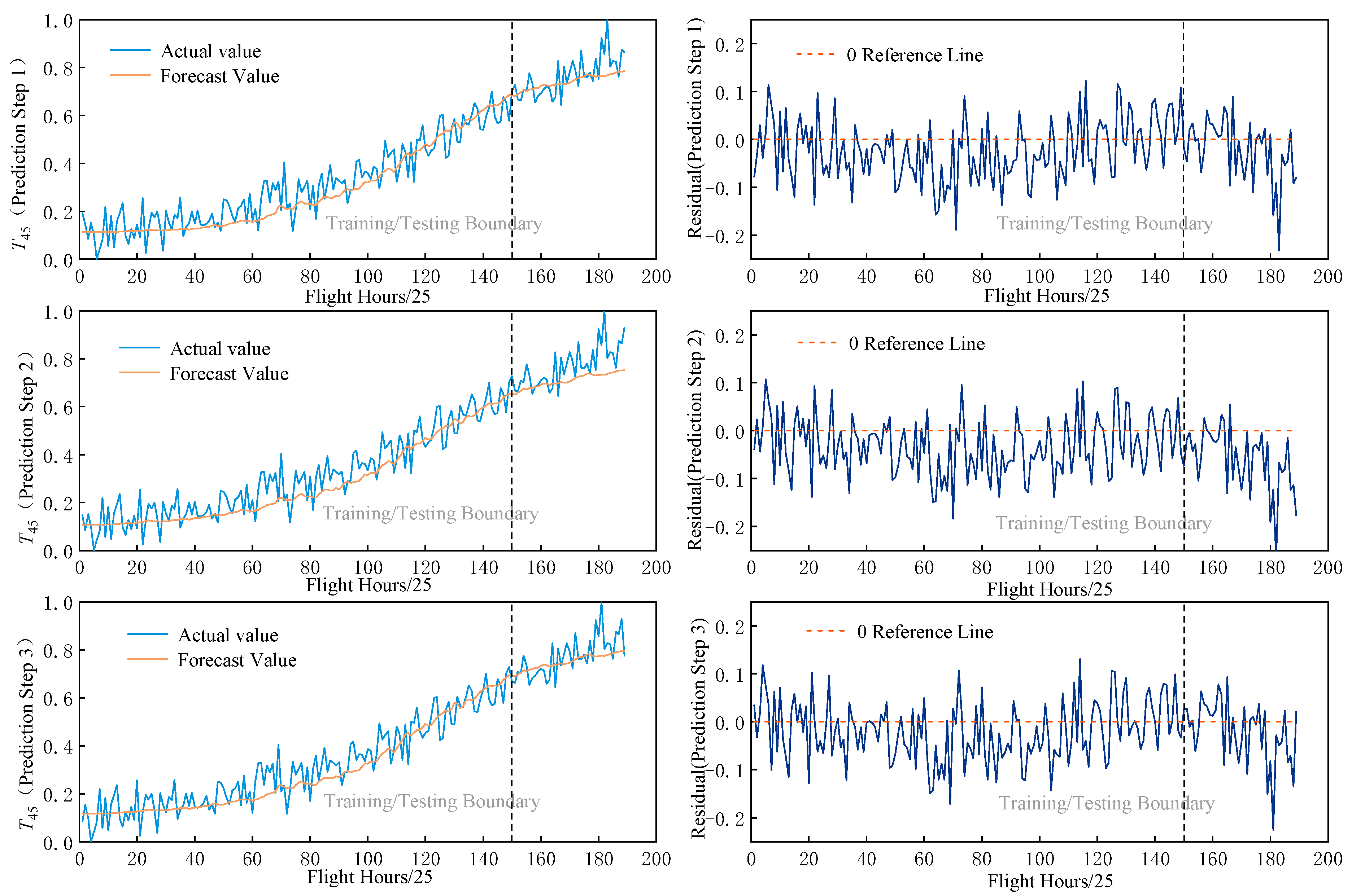
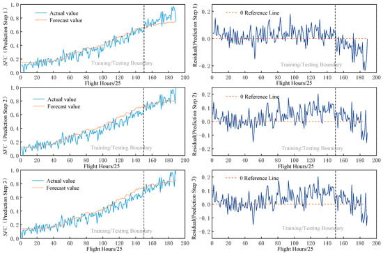
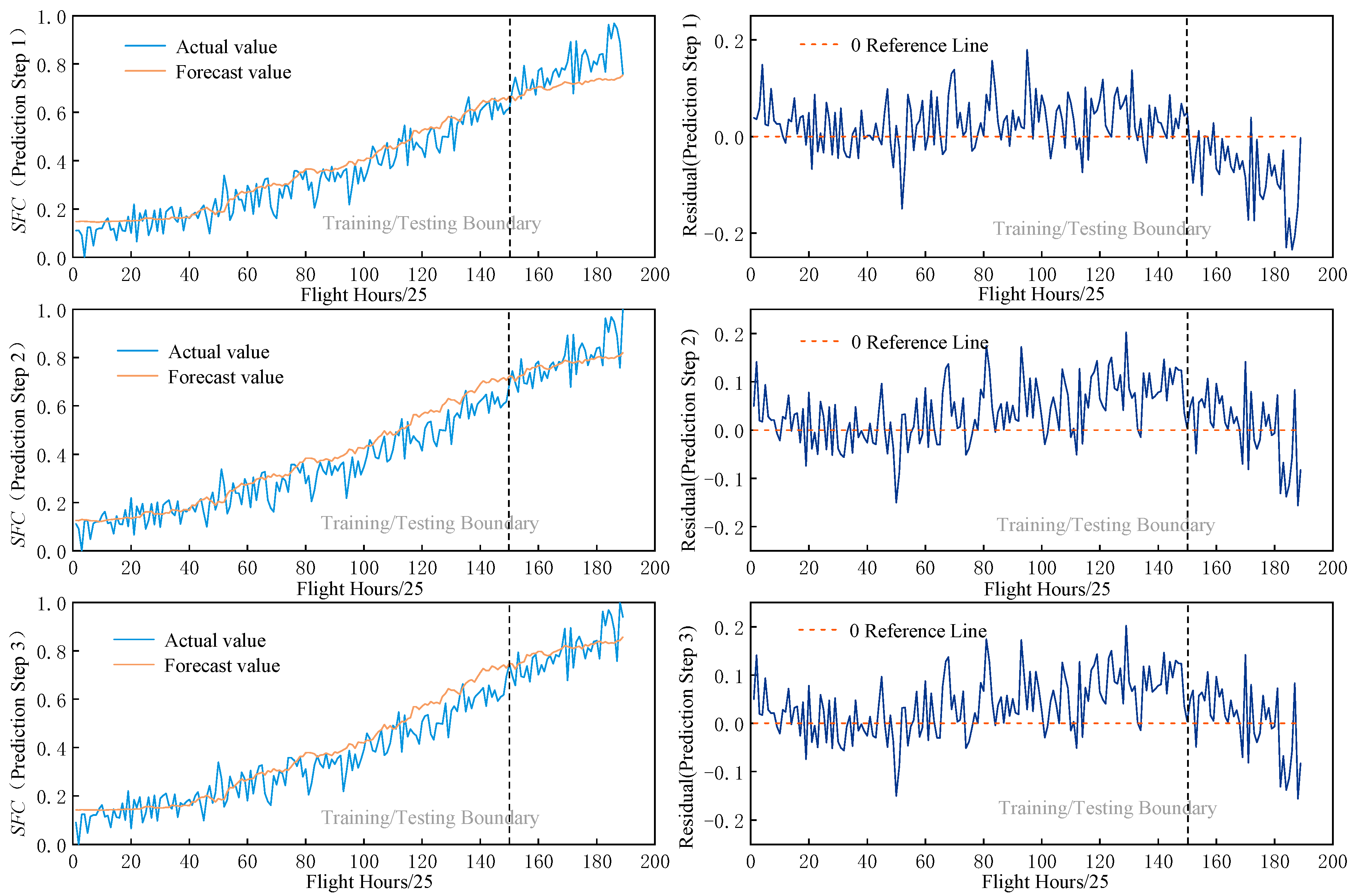
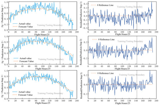
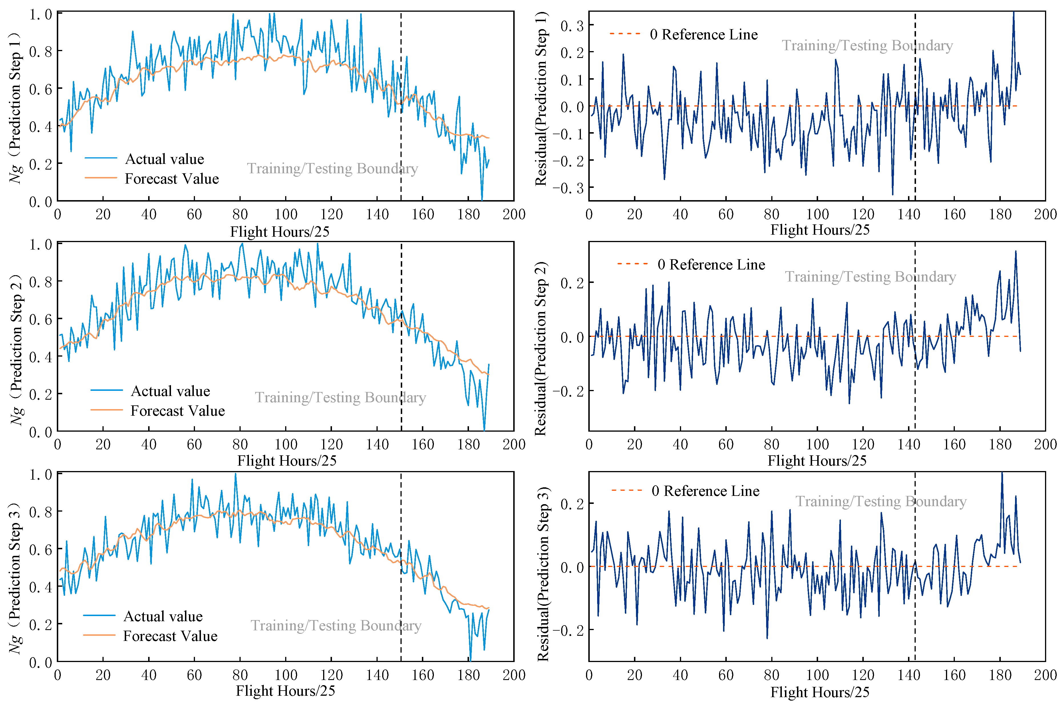
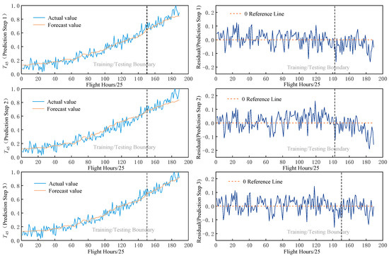
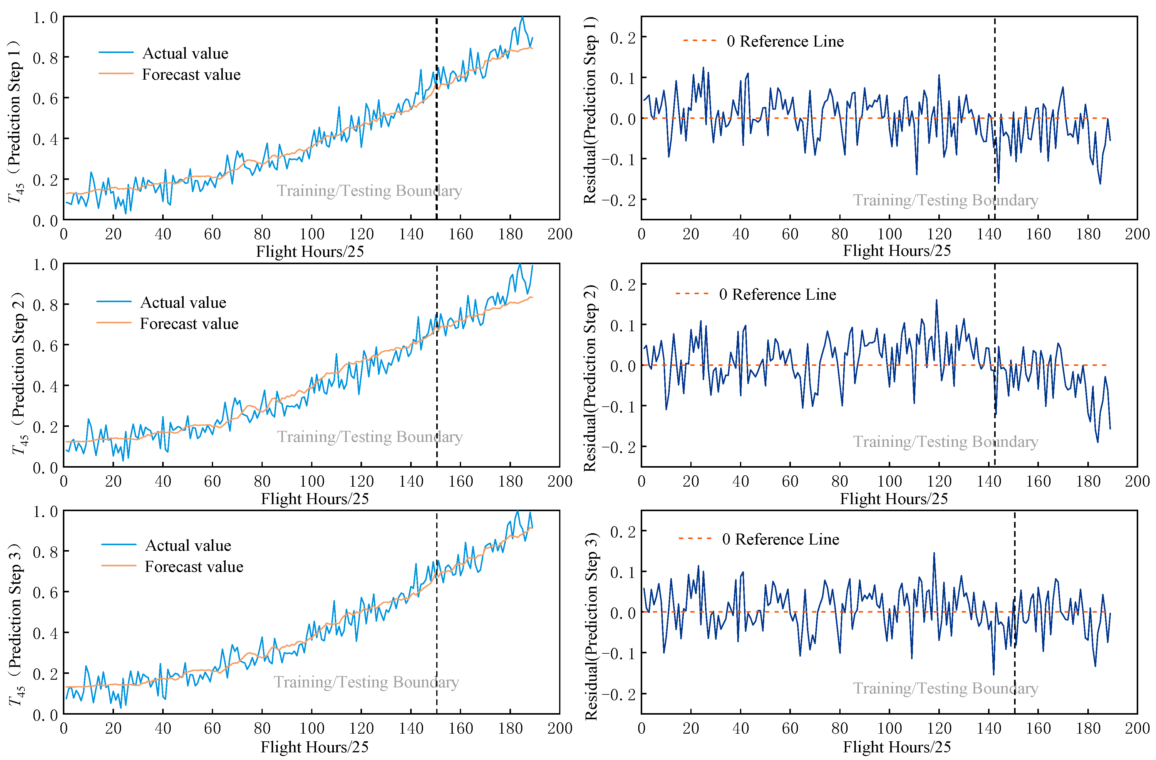
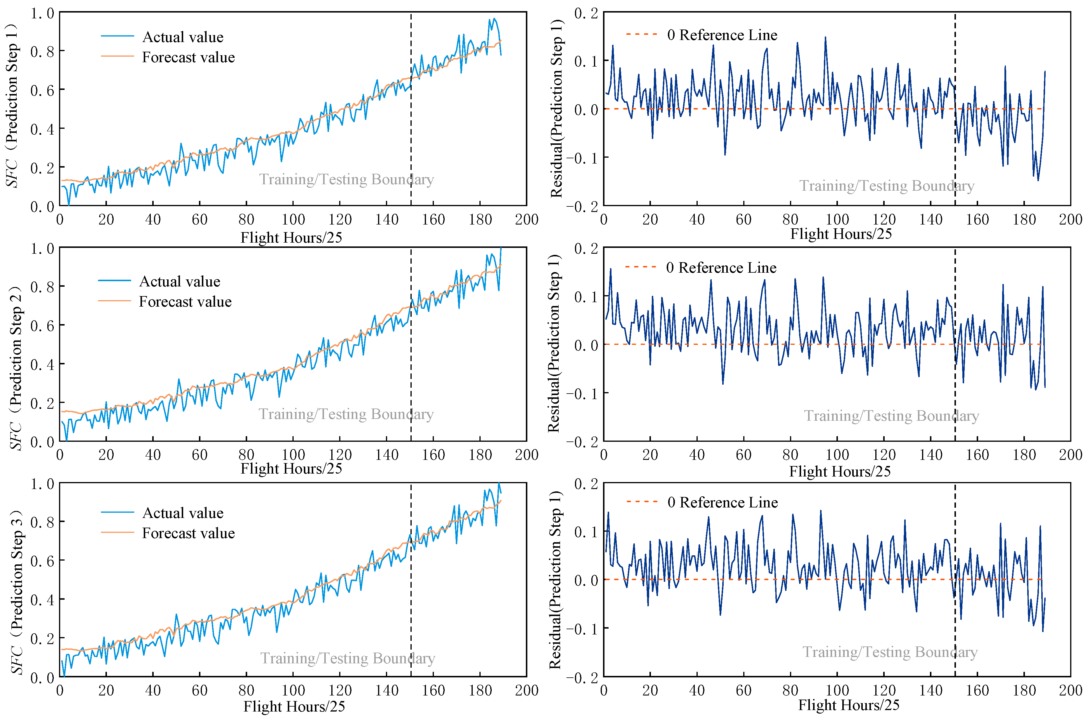
Section 3.1 simulated the degradation process of a turboshaft engine by incorporating deviations in health parameters. Building on this, this section further considers changes in the engine inlet environment by setting different ambient temperatures to simulate non-standard atmospheric conditions and conducts predictive simulations of performance parameters. Under ground conditions (H = 0, Ma = 0, Pa), this section simulates the turboshaft engine’s performance parameters in °C (Environment ①), °C (Environment ②), and °C (Environment ③), and performed predictive simulations of the engine’s overall performance parameters. Since engine performance degradation is a gradual process, data was extracted every 25 flight hours to predict Steps 1–3, corresponding to flight hours of 25, 50, and 75, respectively. The prediction and error curves for Environment ① and ② are shown in Figure 10, Figure 11, Figure 12, Figure 13, Figure 14 and Figure 15. The statistical analysis of prediction errors for the three environments (based on a 3-step forecast) is presented in Table 6.
Figure 10.
Environment ① Ng Prediction Results.
Figure 11.
Environment ① T45 Prediction Results.
Figure 12.
Environment ① SFC Prediction Results.
Figure 13.
Environment ② Ng Prediction Results.
Figure 14.
Environment ② T45 Prediction Results.
Figure 15.
Environment ② SFC Prediction Results.
Table 6.
Statistics on Prediction Errors (Calculated Using the Three-Step Prediction Method).
The simulation results show that the TCN–BiLSTM–Attention hybrid prediction model proposed in this chapter achieved low prediction errors under various inlet conditions. Specifically, the TCN focuses on local dependencies in the time series, the BiLSTM captures long-term dependencies in both forward and backward directions, and the attention mechanism further enhances the model’s ability to extract features at key time steps, enabling the model to accurately capture trends in performance parameters under various operating conditions. In terms of estimation error, the training and testing RMSE values for the three performance parameters remained between 0.05 and 0.09. The training and testing errors were essentially similar, indicating that the model possesses good generalization ability and did not exhibit significant overfitting or underfitting.
B. Multivariate Forecasting of Performance Parameters
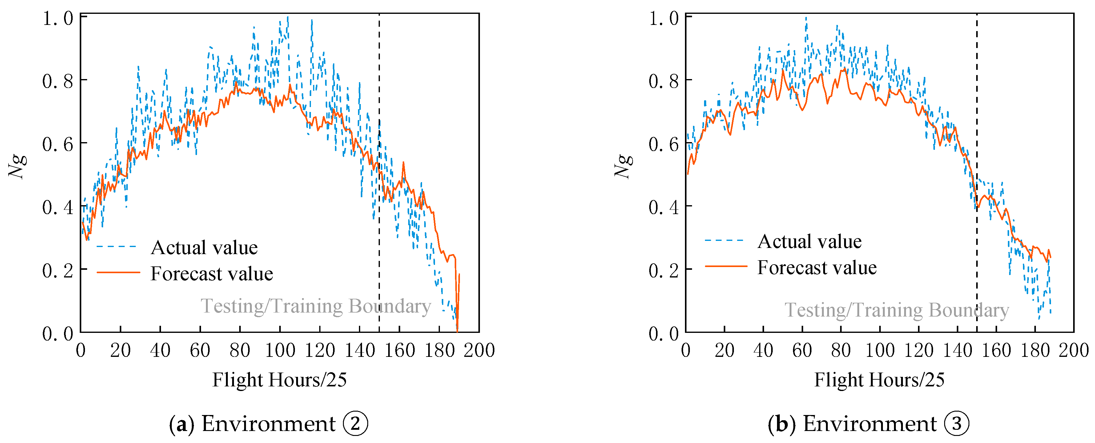
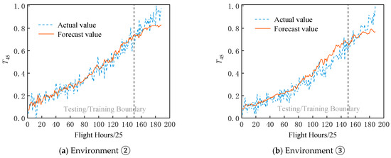
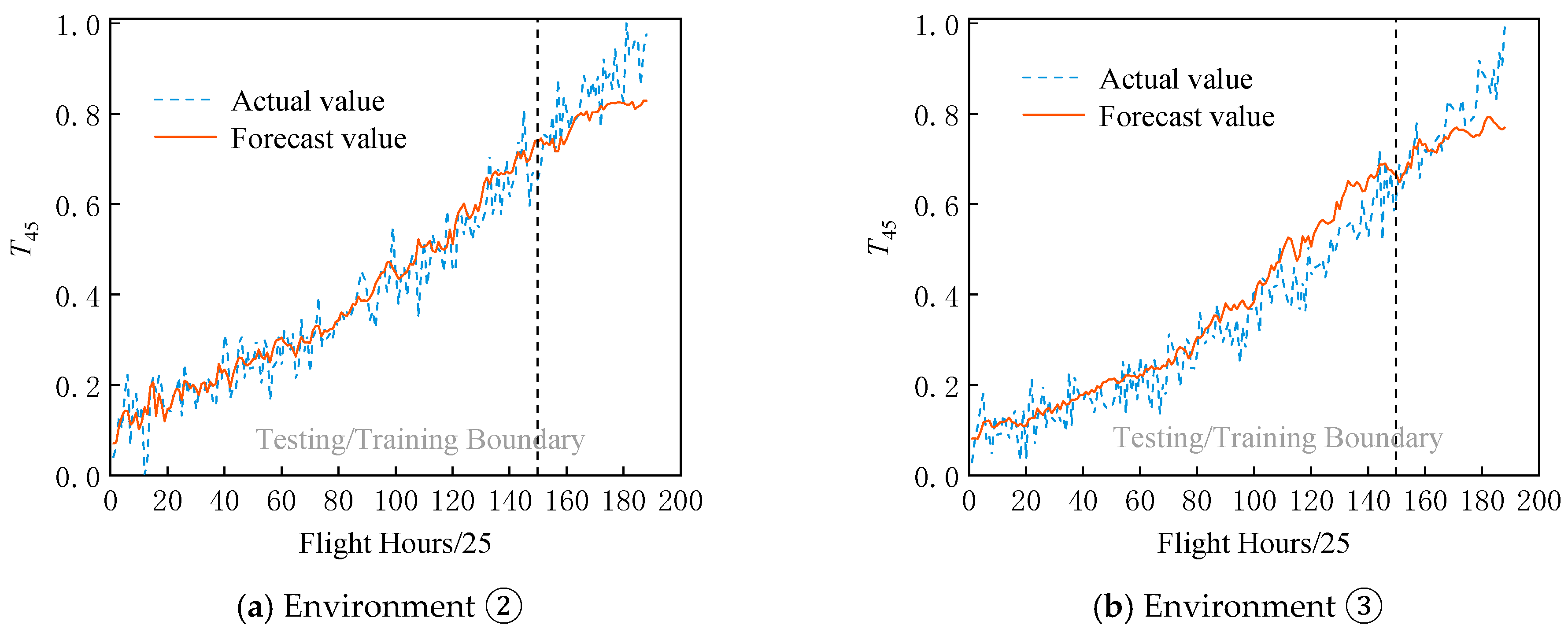
Based on the parametric autoregressive forecasting model established in Section 3.1, as shown in Equation (18), autoregressive forecasting simulations were conducted for the two sets of performance parameters—Ng and T45—under environments ② and ③, respectively, using the TCN–BiLSTM–Attention hybrid algorithm proposed in this chapter under the same simulation conditions. The results are shown in Figure 16 and Figure 17.
Figure 16.
Autoregressive Forecasting of Gas Turbine Speed (Ng).
Figure 17.
Autoregressive Forecasting of Turbine Outlet Temperature (T45).
As shown in Figure 16 and Figure 17, under the autoregressive forecasting mode, the TCN–BiLSTM–Attention hybrid model’s extrapolated predictions of turboshaft engine performance parameters generally track the trends of the actual values well. The predicted curves closely follow the actual values, and their fluctuations are smaller than those of the raw data, indicating that the model has a certain smoothing effect on measurement noise. This is because the dilated convolutional structure of the TCN can stably extract local temporal features. Furthermore, the prediction results show good consistency across different operating conditions, with no instances of significantly increased error under any specific operating condition, indicating that the model possesses good generalization capability regarding changes in inlet temperature. However, it is worth noting that the overall accuracy of autoregressive prediction is lower than that of the multi-parameter input mapping prediction discussed in the previous section. This is because autoregressive prediction relies solely on the historical sequence of the target parameter; the input information is relatively one-dimensional, the available features are limited, and the process is susceptible to cumulative errors and random perturbations during iteration. Nevertheless, overall, the TCN–BiLSTM–Attention model proposed in this chapter maintains relatively stable prediction performance across various task scenarios, validating its applicability in practical engineering. It should be noted that the current validation of the proposed framework is conducted using data generated from a validated component-level turboshaft engine model rather than actual in-service telemetry data. This modeling approach, which simulates performance degradation by introducing deviations in component health parameters, is a standard and widely accepted practice in the aero-engine prognosis literature for initial method validation.
4. Conclusions
To address the challenge of turboshaft engine performance prediction, an attention-enhanced TCN–BiLSTM hybrid model is proposed. The TCN is employed to extract local temporal features, while the BiLSTM captures long-range bidirectional dependencies, enabling comprehensive learning of both local and global temporal representations. An attention mechanism is further incorporated to adaptively weight informative hidden states, thereby emphasizing critical temporal features and improving prediction accuracy. Experimental results on benchmark time-series datasets demonstrate the effectiveness and predictive capability of the proposed framework. The proposed framework is subsequently applied to turboshaft engine performance prediction through two complementary prediction strategies. The first strategy employs a multivariate prediction model that uses sensor measurements related to overall engine performance as inputs. The second strategy adopts a recursive multi-step autoregressive forecasting model based on historical observations of the target parameter. To evaluate model robustness under realistic operating conditions, engine degradation is simulated by introducing deviations into health parameters, and the proposed framework is assessed under non-standard atmospheric conditions. Simulation results indicate that the proposed framework effectively captures the temporal evolution of turboshaft engine performance parameters. Under both prediction strategies, the proposed framework accurately tracks performance parameter variations, effectively suppresses measurement noise, and maintains robust predictive performance under varying operating conditions. The proposed framework therefore provides a reliable foundation for subsequent turboshaft engine health management and remaining useful life (RUL) prediction. It is important to emphasize that current performance degradation models do not yet account for several practical factors, such as maintenance operations, variations during transient maneuvers, and sensor uncertainties. Based on this, we have identified several key directions for future research. First, validation using real-world operational telemetry data is crucial for evaluating the framework’s performance under actual field conditions, which include sensor noise, missing data, and unmodeled dynamic behavior. Second, hybrid physical-information neural networks that integrate physical constraints into the data-driven architecture are expected to further improve prediction accuracy and interpretability. Third, transfer learning and few-shot learning techniques can enable trained models to rapidly adapt to new engine types or individual engines with limited historical data, thereby significantly enhancing the framework’s practical deployability. These research directions represent the logical next step in the transition from simulation-based validation to real-world engineering applications.
Author Contributions
Conceptualization, C.W. and X.Z.; Methodology, C.W. and X.Z.; Validation, C.W. and X.Z.; Writing—original draft, X.Z.; Writing—review and editing, J.C.; Visualization, J.C.; Supervision, J.H. and F.L. All authors have read and agreed to the published version of the manuscript.
Funding
This research received no external funding.
Data Availability Statement
The original contributions presented in this study are included in the article. Further inquiries can be directed to the corresponding author.
Conflicts of Interest
Author Chengjiu Wang was employed by the company Aviation Industry Corporation of China. The remaining authors declare that the research was conducted in the absence of any commercial or financial relationships that could be construed as a potential conflict of interest.
References
- He, D.; Bechhoefer, E.; Hess, A. Automated Rotorcraft Turboshaft Engine Performance Prediction Using a Transfer Learning Approach. In Proceedings of the 2025 IEEE Aerospace Conference, Big Sky, MT, USA, 1–8 March 2025; pp. 1–9. [Google Scholar] [CrossRef] [Scilit]
- Zhou, L. Aero-Engine Health Assessment Based on Data-Driven. Master’s Thesis, Nanjing University of Aeronautics and Astronautics, Nanjing, China, 2022. [Google Scholar]
- Joly, R.B.; Ogaji, S.O.T.; Singh, R.; Probert, S.D. Gas-turbine diagnostics using artificial neural-networks for a high bypass ratio military turbofan engine. Appl. Energy 2004, 78, 397–418. [Google Scholar] [CrossRef] [Scilit]
- Chen, J.M.; Jia, R.; Duan, H. Application of BP Neural Networks in Turboshaft Engine Parameter Conversion. Manuf. Autom. 2022, 44, 31–35. [Google Scholar]
- Tan, W.; Xu, J.; Yu, X.C. Prediction of Aeroengine Performance Deterioration Index Based on Support Vector Machine. Aeroengine 2014, 40, 51–55. (In Chinese) [Google Scholar] [CrossRef]
- Cao, H.L.; Wang, R. Online Prediction of Aircraft Engine Performance Parameters Using Adaptive Support Vector Machines Based on a Sliding Time-Window Strategy. Propuls. Technol. 2020, 41, 1887–1894. [Google Scholar] [CrossRef]
- Vladov, S.; Yakovliev, R.; Bulakh, M.; Vysotska, V. Neural Network Approximation of Helicopter Turboshaft Engine Parameters for Improved Efficiency. Energies 2024, 17, 2233. [Google Scholar] [CrossRef] [Scilit]
- Vladov, S.; Vysotska, V.; Sokurenko, V.; Muzychuk, O.; Peleshchak, R.; Peleshchak, I. Determining Aviation Equipment Malfunctions Type Influence on Neural Network Diagnostic Models Behavior. In Proceedings of the 2024 IEEE 19th International Conference on Computer Science and Information Technologies (CSIT), Lviv, Ukraine, 16–19 October 2024; pp. 1–4. [Google Scholar] [CrossRef] [Scilit]
- Vladova, N.; Vladov, S.; Sachenko, A.; Wolff, C.; Kochan, V.; Pytel, S.; Sapozhnyk, G. Intelligent Algorithm for Indirect Measuring the Gas Temperature of Helicopter Turboshaft Engines’. In Proceedings of the 2025 IEEE 13th International Conference on Intelligent Data Acquisition and Advanced Computing Systems: Technology and Applications (IDAACS), Gliwice, Poland, 4–6 September 2025; pp. 1–6. [Google Scholar] [CrossRef] [Scilit]
- Dong, Q.; Li, B.W.; Yan, S.Q.; Qian, R.J. Prediction of Performance Parameters During the Acceleration Process of a Turboshaft Engine Based on BSO-ELM. Syst. Eng. Electron. 2021, 43, 2181–2188. [Google Scholar]
- Song, Y.F.; Zhao, S.; Lu, F.; Jiang, C.Y. The Power Estimation of Turboshaft Based on Kmeans-ELM Method. In Proceedings of the 6th China Aviation Science and Technology Conference; Beihang University Press: Beijing, China, 2023; pp. 1314–1322, (In Chinese). [Google Scholar] [CrossRef]
- Andrianantara, R.P.; Ghazi, G.; Botez, R.M. Performance model identification of the general electric CF34-8C5B1 turbofan using neural networks. J. Aerosp. Inf. Syst. 2023, 20, 831–848. [Google Scholar] [CrossRef] [Scilit]
- Wang, L.; Chen, Y.; Zhao, X.; Xiang, J. Predictive Maintenance Scheduling for Aircraft Engines Based on Remaining Useful Life Prediction. IEEE Internet Things J. 2024, 11, 23020–23031. [Google Scholar] [CrossRef] [Scilit]
- Dan, Y.; Zhang, M.; Wang, Z.; Sun, C. Spike-TCN with Depthwise-Separable Convolution and Attention for Efficient Time Series Prediction. Int. J. Comput. Intell. Syst. 2025, 18, 312. [Google Scholar] [CrossRef] [Scilit]
- Li, J.; Jia, Y.; Niu, M.; Zhu, W.; Meng, F. Remaining Useful Life Prediction of Turbofan Engines Using CNN-LSTM-SAM Approach. IEEE Sens. J. 2023, 23, 10241–10251. [Google Scholar] [CrossRef] [Scilit]
- Dida, M.A.; Cheriet, A.; Belhadj, M. Remaining Useful Life Prediction Using Attention-LSTM Neural Network of Aircraft Engines. Int. J. Progn. Health Manag. 2025, 16, 1–12. [Google Scholar] [CrossRef] [Scilit]
- Yang, W.; Zhou, Q.; Chen, G.; Liu, C.; Qu, C. SDPA-BiLSTM: Improving Accuracy of Aircraft Engine Remaining Life Prediction with Enhanced Attention Mechanism. In Proceedings of the 2024 9th International Conference on Computer and Communication Systems (ICCCS), Xi’an, China, 19–22 April 2024; pp. 569–574. [Google Scholar] [CrossRef] [Scilit]
- Zhu, Z.; Tao, J.; Zhang, C.; Ma, Y.; Huang, C.; Qiu, F. Hybrid CNN-BiLSTM Model with Simulated Annealing Optimization for Aircraft Engine RUL Prediction. In Proceedings of the 2025 5th International Conference on Electronic Information Engineering and Computer Science (EIECS), Changchun, China, 26–28 September 2025; pp. 400–404. [Google Scholar] [CrossRef] [Scilit]
- Wang, J.; Wang, Y.; Li, J. Interpretable and efficient RUL prediction of turbofan engines using EM-enhanced Bi-LSTM with TCN and attention mechanism. Eng. Res. Express 2024, 6, 035507. [Google Scholar] [CrossRef] [Scilit]
- Deng, S.; Zhou, J. Prediction of remaining useful life of aero-engines based on CNN-LSTM-attention. Int. J. Comput. Intell. Syst. 2024, 17, 232. [Google Scholar] [CrossRef] [Scilit]
- Du, W.; Zhang, J.; Meng, G.; Zhang, H. Aero-Engine Fault Detection with an LSTM Auto-Encoder Combined with a Self-Attention Mechanism. Machines 2024, 12, 879. [Google Scholar] [CrossRef] [Scilit]
- Xiao, G.; Jin, C.; Bai, J. Remaining Useful Life Prediction for Aero-Engines Based on Multi-Scale Dilated Fusion Attention Model. Appl. Sci. 2025, 15, 9813. [Google Scholar] [CrossRef] [Scilit]
- Bai, S.; Kolter, J.Z.; Koltun, V. An empirical evaluation of generic convolutional and recurrent networks for sequence modeling. arXiv 2018, arXiv:1803.01271. [Google Scholar]
- Graves, A.; Fernández, S.; Schmidhuber, J. Bidirectional LSTM Networks for Improved Phoneme Classification and Recognition. In International Conference on Artificial Neural Networks; Springer: Berlin/Heidelberg, Germany, 2005; pp. 799–804. [Google Scholar]
- Bahdanau, D.; Cho, K.; Bengio, Y. Neural machine translation by jointly learning to align and translate. arXiv 2014, arXiv:1409.0473. [Google Scholar]
- Nair, V.; Hinton, G.E. Rectified linear units improve restricted boltzmann machines. In Proceedings of the 27th International Conference on Machine Learning (ICML-10), Haifa, Israel, 21–24 June 2010; pp. 807–814. [Google Scholar]
- Salimans, T.; Kingma, D.P. Weight normalization: A simple reparameterization to accelerate training of deep neural networks. arXiv 2016, arXiv:1602.07868. [Google Scholar]
- Hinton, G.E.; Srivastava, N.; Krizhevsky, A.; Sutskever, I.; Salakhutdinov, R.R. Improving neural networks by preventing co-adaptation of feature detectors. arXiv 2012, arXiv:1207.0580. [Google Scholar]
- Wang, C.; Zhu, X.; Zhou, X.; Huang, J.; Lu, F. Performance Monitoring Based on Improved Adaptive Kalman Filtering for Turboshaft Engines Under Network Uncertainties. Aerospace 2025, 12, 241. [Google Scholar] [CrossRef] [Scilit]
- Jonathan, A.; Jonathan, S.; Dean, K. A Modular Aero-Propulsion System Simulation of a Large Commercial Air-Craft Engine; NASA-TM-2008-215303; NASA Glenn Research Center: Cleveland, OH, USA, 2007. [Google Scholar]
- Tong, Z. A Study on Intelligent Diagnostic Technology for Air System Faults in Turboshaft Engines. Master’s Thesis, Nanjing University of Aeronautics and Astronautics, Nanjing, China, 2021. [Google Scholar]

Disclaimer/Publisher’s Note: The statements, opinions and data contained in all publications are solely those of the individual author(s) and contributor(s) and not of MDPI and/or the editor(s). MDPI and/or the editor(s) disclaim responsibility for any injury to people or property resulting from any ideas, methods, instructions or products referred to in the content. |
© 2026 by the authors. Licensee MDPI, Basel, Switzerland. This article is an open access article distributed under the terms and conditions of the Creative Commons Attribution (CC BY) license.