


Abstract
Flow-field parameters of bow shocks in high-altitude rarefied flow are fundamental for seeker radiation noise evaluation and thermal-protection design. The conventional direct simulation Monte Carlo (DSMC) method is computationally expensive, making it difficult to achieve real-time prediction and massive sample generation of flow-field parameters. This paper presented a surrogate model adopting a convolutional neural network (CNN) to rapidly predict bow-shock reactive flow-field parameters. A blunt body with a nose radius of 0.1–1.0 m was investigated. The Latin hypercube sampling methodwas used to construct a sample space spanning altitudes of 80–150 km and Mach numbers of 15–35. DSMC-calculated data was segmented into training and test sets at a ratio of 4:1 and verified by the bow-shock ultraviolet experiments. An encoder–decoder CNN with a parallel decoder strategy was established to develop a bow-shock reactive flow surrogate model (CNN-BS) and conduct error evaluation. The results show that the mean absolute percentage errors for temperature, velocity, pressure, and nitric oxide number density are below 8%, with coefficients of determination close to 1. The average prediction time is 0.5 s, enabling online data generation. The CNN-BS model provides efficient support for radiation-noise evaluation and thermal-protection design of hypersonic blunt bodies.
1. Introduction
For a hypersonic blunt body flying in a high-altitude rarefied flow regime, the gas near the nose is severely compressed, thus causing a bow shock to be formed. Significant thermochemical non-equilibrium effects occur in the shock layer [1]. The gas temperature in the shock layer can reach tens of thousands of Kelvin [2]. Complex physicochemical changes, including the dissociation, ionization, and radiation of air molecules, occur in the shock layer [3]. These changes modify the thermodynamic and transport properties of the gas, thus affecting the thermal environment and radiation-noise level at the nose of the blunt body. Therefore, the prediction of bow-shock reactive flow-field parameters under complex physicochemical processes is fundamental to the thermal-protection design and optical-seeker system optimization of hypersonic blunt bodies [4].
The gas temperature and species concentration in the bow-shock layer are essential physical parameters for predicting the radiation noise of optical seekers. For instance, the United States conducted two bow-shock ultraviolet (BSUV) flight tests in the 1990s [5,6]. The BSUV-II test, which was performed at altitudes of 70–90 km and a velocity of 5.1 km/s, validated the reliability of bow-shock radiation calculation data [6]. Specifically, the DSMC method was employed to calculate bow-shock flow-field parameters. Subsequently, the radiative properties of various gases were determined using the non-equilibrium thermodynamic temperatures and mass fractions of dissociated air species. Studies have shown that nitric oxide (NO) is one of the primary species contributing to infrared and ultraviolet radiation in shock flow fields [7]. Boyd [8] proposed a conservative weighted scheme for trace species that resolved the difficulties of momentum and energy conservation as well as computational efficiency in the DSMC simulation of trace NO species in the shock layer. This scheme was subsequently coupled with multiphysics models to analyze NO ultraviolet radiation in the BSUV-II bow-shock flow field [9]. Levin et al. [10] improved the prediction accuracy of NO ultraviolet radiation by modifying the temperature representation of a NO excited-state population model. Karpuzcu et al. [11] implemented NO infrared radiation modeling in hypersonic flows by coupling the DSMC method with a collisional-radiative model. Sun et al. [12] investigated the ultraviolet-radiation characteristics of gases under high-altitude hypersonic conditions by combining a three-temperature model and the DSMC method. They identified the critical effects of temperature and number densities of species, such as NO, on the radiative intensity.
The physicochemical mechanisms governing bow-shock flow fields at altitudes above 80 km are complex and involve significant rarefied gas effects as well as thermal and chemical non-equilibrium [13,14]. By performing DSMC numerical simulations, Cimini et al. [15] demonstrated that high-altitude rarefaction effects can significantly modify both the shock structure and drag characteristics of spacecraft. Shi et al. [16] showed that chemical non-equilibrium in the shock layer contributes significantly to the determination of species concentrations and their spatial distributions. Candler [17] compared the predictions of various high-temperature gas models for bow-shock flow fields and emphasized the necessity of incorporating both thermal and chemical non-equilibrium effects into the gas models. Niu et al. [18] compared the flow field and NO production in a bow-shock layer using a two-temperature model based on three chemical models with different control temperature index assignments. They indicated that the chemical-rate model and control-temperature weighting factor significantly affected the thermochemical non-equilibrium characteristics of the bow-shock flow field. Numerical investigations by Li et al. [19] on bow-shock flow fields at high Mach numbers indicated that thermochemical non-equilibrium significantly affected flow-field parameters. Such non-equilibrium is primarily reflected in the difference between the translational–rotational and vibrational temperatures.
Currently, the DSMC method is commonly employed to calculate bow-shock flow-field parameters in high-altitude flow regimes [14,15]. Its fundamental principle is to solve the Boltzmann equation by monitoring the motions and collisions of numerous simulated molecules [20]. Flow-field calculations based on the DSMC method are extremely time-consuming [21]. Scanlon et al. [22] used the DSMC code “dsmcFoam” to simulate a two-dimensional hypersonic flow around a circular cylinder at Mach and Knudsen numbers of 10 and 0.01, respectively. The simulation was performed on a single Pentium IV 3 GHz processor with a computational time of approximately 36 h. Norman et al. [23] applied the classical trajectory calculation DSMC method, which required several days to compute a one-dimensional nitrogen shockwave model on a single-core CPU. Tumuklu et al. [24] simulated bow shock over a double-wedge model using the DSMC method in a parallel-computing environment with 512 processors, which required approximately 141,000 CPU h. Limited by its low computational efficiency, the DSMC method is only suitable for offline calculations in engineering applications and cannot satisfy the requirements of batch computation and rapid prediction.
In recent years, the successful application of deep learning to flow-field reconstruction has provided a new approach for the real-time prediction of high-altitude shock flow-field parameters [25]. Jin et al. [26] developed a hybrid convolutional neural network (CNN) architecture to reconstruct the velocity field of flows around a cylinder over a wide range of Reynolds numbers using surface pressure data. Hasegawa et al. [27] proposed a reduced-order model that combined a CNN autoencoder and long short-term memory. This model compresses high-dimensional flow-field data while maintaining prediction accuracy, with a prediction error below 5% for the velocity field over new blunt body shapes, thereby providing an efficient tool for complex flow control. Cai et al. [28] combined CNN with the DSMC method to construct an intelligent CNN-DSMC model for rarefied plume flows near the lunar surface, thereby enabling the efficient prediction of plume flow velocity at high altitudes. These studies demonstrate that deep learning can effectively capture the nonlinear mapping relationships among flow-field parameters and is suitable for the rapid prediction of various complex flow problems.
Nevertheless, current research on CNN-DSMC still exhibits notable limitations. Most existing models are restricted to vacuum plumes and chemically inert rarefied flows, covering only a narrow range of predicted parameters. They fail to capture three-temperature thermal non-equilibrium effects and multi-component chemical reaction mechanisms that characterize hypersonic flow at high altitudes [28,29]. Meanwhile, conventional flow field prediction networks typically adopt a single-branch encoder–single-decoder architecture and are trained with globally unified hyperparameters [30]. Such architectures are ill-suited to rarefied reactive flows, where multiple physical quantities exhibit sharply different gradients and drastic variations in magnitude. Moreover, classic models such as U-Net and convolutional autoencoders tend to generate redundant features when resolving thin bow shocks, thereby distorting fine shock structures [31]. Although neural operators represented by DeepONet offer excellent global fitting capability, they suffer from low inference efficiency during simultaneous multi-parameter prediction, failing to meet the requirements of fast engineering computations [32].
Therefore, this study focuses on the rapid prediction of reactive flow-field parameters in a high-altitude rarefied bow-shock layer. In particular, the non-equilibrium temperature, concentration, and distribution of NO species are prioritized. By employing a CNN combined with high-fidelity DSMC data, a rapid prediction model is developed for the reactive bow-shock flow field around blunt bodies over a wide velocity range at high altitudes. The model enables rapid predictions from blunt-body geometric parameters to bow-shock flow-field parameters.
2. Physical Models and Numerical Methods
2.1. Boltzmann Equation
In hypersonic flows within the rarefied flow regime, the Knudsen number is relatively high. Therefore, the rarefaction and thermochemical non-equilibrium effects of the gas medium must be considered. In this case, the governing equation is the Boltzmann equation, which describes the evolution of the gas molecular velocity distribution function , i.e.,
where is the position vector, is the velocity vector, and is the external force acceleration. The right-hand side collision term represents the effect of intermolecular collisions on the velocity distribution function.
In hypersonic rarefied flows, intermolecular attractive forces are negligible and the variable soft sphere (VSS) model [20] is employed to describe the collision dynamics. In this case, the intermolecular interaction potential can be represented by an inverse power-law model, and the right-hand side collision term is:
where is the cutoff value of the collision parameter, a is the inverse power law constant, α is the inverse power law exponent, is the reduced mass, and g is the relative velocity of gas molecules.
2.2. DSMC Method
The DSMC method approximates the solution of the Boltzmann equation by simulating the motion and collisions of computational particles. First, within a time step , molecules propagate freely:
where and denote the position and velocity of the molecule at step n, respectively. is the position at step n + 1.
Subsequently, the collision particle pairs are selected within each grid cell using the no time counter method [20]. For a grid cell containing N computational particles, let the position and velocity of simulated particle i be and , respectively. Thus, the collision probability between any two simulated particles i and j is expressed as:
where C is a proportionality constant related to the number of particles N in the cell, the time step , and the cell volume V.
As the Boltzmann equation only accounts for binary collisions, both momentum and energy are conserved in elastic collisions:
where mi and mj are the masses of two simulated particles i and j, respectively. and represent their pre-collision velocities, respectively. and represent the corresponding post-collision velocities, respectively. is the center-of-mass velocity of the particle pair.
Thus, the post-collision velocities of the particles are expressed as:
where denotes the post-collision relative velocity of the particles. Substituting into the equations yields the updated particle velocities and . DSMC simulations in this work are performed using Stochastic PArallel Rarefied-gas Time-accurate Analyzer (SPARTA) [33].
2.3. Chemical Reaction Model
Complex chemical reactions occur within the shock layer, which can be described by the total collision energy (TCE) model proposed by Bird [20,34]. A chemical reaction occurs if the total collision energy Ec of the colliding pair exceeds the activation energy Ea required for the reaction. The reaction probability P is defined as the ratio of the reaction cross-section to the total collision cross-section, i.e.,
where is the total collision cross-section. is the symmetry factor, which assumes the value of 2 for collisions between identical molecules and 1 otherwise. is the reference temperature, is the gamma function, is the average internal degrees of freedom, is the average viscosity exponent, and is the reduced mass. Here, A, k, and b are given by the Arrhenius equation:
where k is the Boltzmann constant. A and b are constants determined experimentally.
2.4. Macroscopic-Parameter Representation
A statistical steady state was first achieved, and the macroscopic flow parameters were obtained by statistically averaging all the particles in each grid cell. The density ρ, temperature T, and velocity ν are expressed as:
In thermochemical non-equilibrium flows in the shock layer, energy exchange among the translational, rotational, and vibrational modes can exhibit significant relaxation lags. This necessitates the use of distinct temperature definitions for each mode:
where is the macroscopic velocity vector, with , , being the velocity components in the x, y, and z directions, respectively. is the average molecular mass. and denote rotational and vibrational degrees of freedom, respectively. and denote the rotational and vibrational energies of a single molecule, respectively.
2.5. CNN Model
The core role of a CNN in surrogate-model construction is to automatically extract and encode the spatial structural information of flow fields via convolutional operations. By mapping physical parameters into hierarchical features through convolutional kernels, the CNN establishes efficient mapping from simple input conditions to complex flow-field distributions. For an input matrix X and a convolutional kernel K, the convolutional operation [35] is
where O is the output matrix. b is the bias constant applied to all the output positions. i and j are the row and column indices of the output matrix O, respectively. m and n are the row and column indices of the convolution kernel K, respectively. The height and width of the output matrix are expressed as:
where and are the height and width of the input matrix, respectively. p is the padding size, k is the convolution kernel size, and s is the stride.
The features extracted via convolution require a nonlinear transformation to enhance the expressive power of the model. The rectified linear unit (ReLU) activation layer operates on each input element. It preserves the positive unmodified values and sets the negative values to zero. This operation effectively alleviates the vanishing-gradient problem caused by negative outliers and improves the computational efficiency [36].
A batch normalization layer is introduced after the activation layer to further accelerate convergence. This layer normalizes the distribution of each mini-batch to a standard normal distribution with zero mean and unit variance. For an input feature set with batch size B, the mean μ and variance σ2 are expressed as:
where is the input feature value and b is the batch index. Subsequently, the normalization and transformation reconstructions are expressed as:
where γ and β are the scaling and shifting parameters, respectively. ε is a numerical stability constant and is the normalized output feature value.
The convolution block is followed by a max-pooling layer, which reduces the overall computational load. Downsampling is implemented in this layer to extract local maxima from the feature maps. Thus, the feature dimensionality is reduced, whereas the key dominant features are retained. This operation inevitably causes a partial loss of spatial information. Subsequently, the deconvolution layers are used to upsample the pooled feature maps. The input dimensions are restored using a predefined transposed convolution kernel and stride. A deconvolution kernel is generated by centrally flipping the original convolution kernel. The height and width of the output matrix yielded by the deconvolution operation are:
where the symbol “∗” denotes parameters associated with the deconvolution operation.
The final stage integrates a fully connected layer behind the deconvolution block. The weights and biases are learned within this layer to support global feature integration. The high-dimensional features from the preceding deconvolution layers serve as the input. Feature decoding and model reconstruction are completed via the formula:
where y is the output vector, f(x) is the activation function, w is the weight matrix, x is the input vector, and b is the bias matrix.
2.6. Error Evaluation Metrics
Network training realizes the iterative optimization of the model parameters through backpropagation and gradient descent. The mean absolute percentage error (MAPE) [37] is adopted as the loss function:
where is the number of samples, is the predicted value for sample i, and is the actual value for sample i.
The gradients of the loss function with respect to the parameters of each layer are calculated via backpropagation. Subsequently, the gradient-descent method is employed to iteratively update the weights w and biases b. This process gradually approaches the optimal solution. The update formulas for the weights and biases, respectively, are as follows [38]:
where t is the iteration epoch and η is the initial learning rate.
The prediction accuracy of the model under unknown operating conditions is evaluated using the coefficient of determination R2 as the evaluation metric:
where is the mean of all the actual values. As R2 approaches 1 and the MAPE approaches 0, the prediction accuracy of the model improves.
3. Construction of CNN-Based Surrogate Model
3.1. Data Generation and Preprocessing
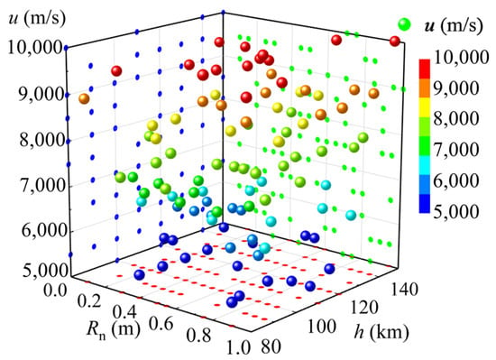
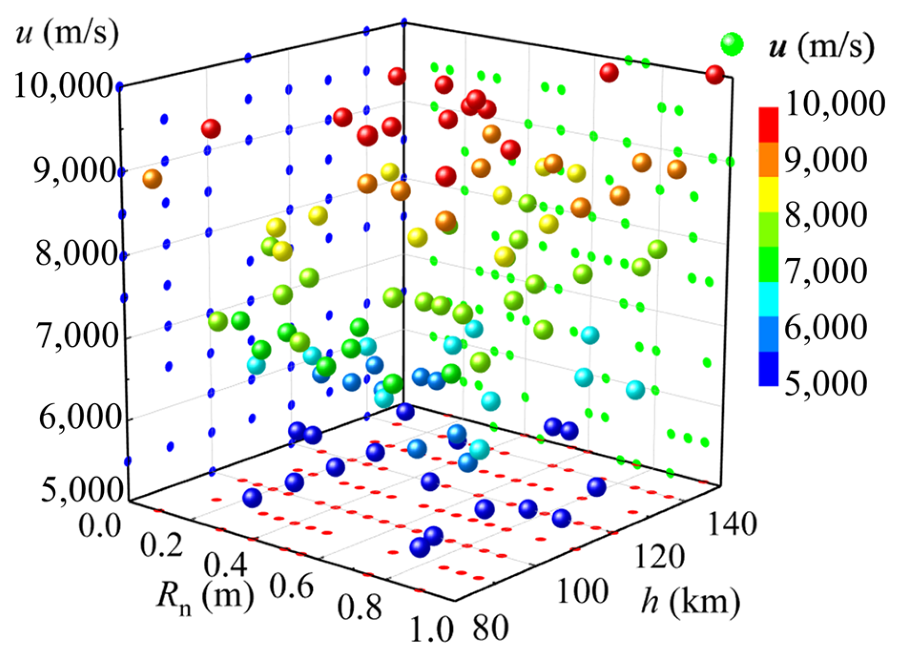
Sample points were selected uniformly within the parameter space to construct a surrogate model applicable to hypersonic bow-shock flow fields at high altitudes. The Latin hypercube sampling (LHS) method was used for sample generation in this study. Three key parameters governing the shock-layer characteristics were identified: nose radius, flight altitude, and flight velocity. Their respective value ranges are listed in Table 1, and the overall Knudsen number of all cases varies from 0.004 to 325, representing obvious rarefied gas effects. A total of 100 sample points were generated. The nose radius was discretized from 0.1 to 1.0 m at an interval of 0.05 m. The flight altitude and flight velocity were sampled continuously within their corresponding ranges. The LHS method ensured uniform sample coverage across all parameter dimension and enabled random combinations of diverse parameters. The distribution of the generated samples is shown in Figure 1. Satisfactory uniformity was observed for all the parameters within their design ranges, with no significant clustering.
Table 1.
Parameter sampling range.
Figure 1.
Distribution of sampling points generated by LHS for nose radius, flight altitude and flight velocity.
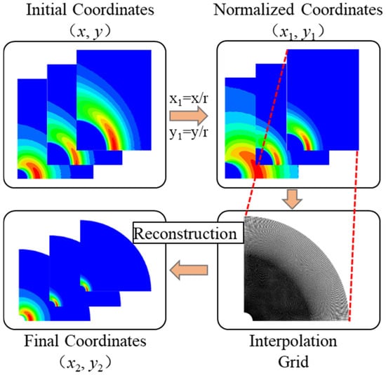
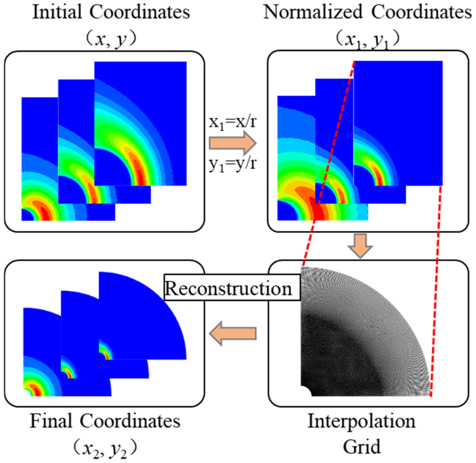
All the sampled operating conditions were subjected to DSMC numerical simulations to acquire the original flow-field data. Subsequently, the flow-field information obtained was processed using a dedicated preprocessing procedure. The computational domain was non-dimensionalized based on the nose radius. Such an operation effectively removed feature redundancies and scale discrepancies caused by variations in the radius. Consequently, the generalizability of the model was enhanced and the risk of overfitting was significantly reduced. The reconstruction of dimensionless flow-field data using different samples was conducted to unify the input format of the CNN. An inverse distance-weighting interpolation scheme was employed to map all the sample data onto a unified fixed grid. The overall data pre-processing workflow is shown in Figure 2. This step normalized the computational domain and maintained the consistency of the grid nodes.
Figure 2.
Schematic diagram of data preprocessing.
To address the issue that the NO number density tends to approach zero and thereby causes instability in the MAPE calculation, an additional numerical treatment step was introduced. Cells with a number density below 1 × 10⁷ throughout the domain were uniformly assigned a value of 1 × 10⁷, and a logarithmic transformation was subsequently applied to the NO number density. This compressed the dynamic range of the data and avoided numerical anomalies.
A structured dataset was established via the aforementioned preprocessing operations. Each sample comprised a multidimensional array containing multiple physical fields, including the translational temperature, rotational temperature, vibrational temperature, pressure, velocity, and NO number density. These variables were defined on a unified grid. In total, 80% of the samples in the dataset were allocated to the training set for supervised learning to minimize the loss function during neural-network training. The remaining 20% of the samples were designated as the test set to predict the flow-field properties under unknown operating conditions. This test set was further utilized to evaluate the generalization performance of the trained model on unseen samples.
In this study, only the NO number density was selected as the primary species for analysis. As noted in the introduction, NO is the most dominant radiating species in hypersonic rarefied bow-shock flow fields, and its radiation characteristics are central to seeker radiation noise assessment and thermal protection design. Furthermore, under high-altitude thermochemical non-equilibrium, the concentration and spatial distribution of NO are highly sensitive to variations in temperature, velocity, and pressure. As such, they can effectively capture the chemical evolution within the shock layer and the overall characteristics of the non-equilibrium flow.
3.2. Sample-Data Validation
The reliability of the DSMC numerical model was validated through comparison with simulation data for the BSUV-II forebody flow at an altitude of 80 km [8]. Numerical simulations were performed using a two-dimensional axisymmetric simplified model, with the blunt-body nose represented as a quarter-circle. The computational domain was 0.4 × 0.5 m. An 80 × 100 baseline grid was used, with a two-level mesh hierarchy and near-wall refinement to better resolve the boundary layer and shock regions. The initial time step was 2.1 × 10⁻⁷ s. Freestream conditions followed the standard atmosphere at 80 km altitude. The gas mixture comprised 11 species: O2, N2, O, N, NO, and their associated ions and electrons. A total of 1 × 10⁶ simulated particles were used, satisfying the statistical accuracy requirements for rarefied flows. At the inflow boundary, particles were injected at the freestream velocity and temperature given in the literature. The wall was modeled as a diffuse reflector at 300 K with full accommodation. The lower y-axis boundary was treated as axisymmetric, and the remaining outer boundaries were set as free outflow. Simulations were executed using a domain-decomposition message passing interface (MPI) parallel strategy.
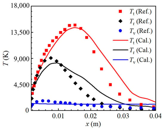
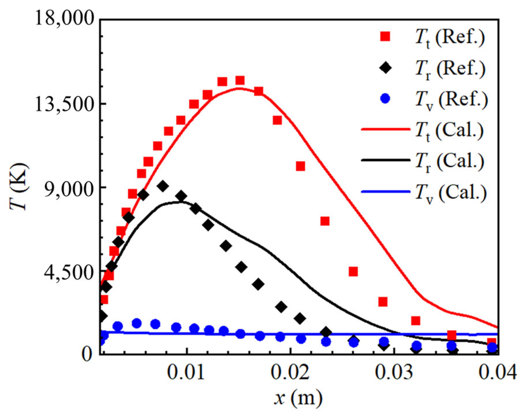
Numerical simulations were performed using the VSS and TCE models. The computed translational temperature Tt, rotational temperature Tr, and vibrational temperature Tv were compared with reference data. Figure 3 shows a comparison of the temperature profiles along the stagnation line. Good agreement was achieved between the present results and reference data, with a peak error below 10%. The differences between the translational, rotational, and vibrational temperature curves revealed strong thermal non-equilibrium effects inside the bow-shock layer. The validity of the adopted DSMC approach was confirmed by the results above. The generated sample data exhibited satisfactory credibility and were applicable to subsequent machine-learning modeling and analysis.
Figure 3.
Comparison of translational, rotational and vibrational temperature profiles along the stagnation line between present DSMC results and reference data.
3.3. CNN-BS Model Construction
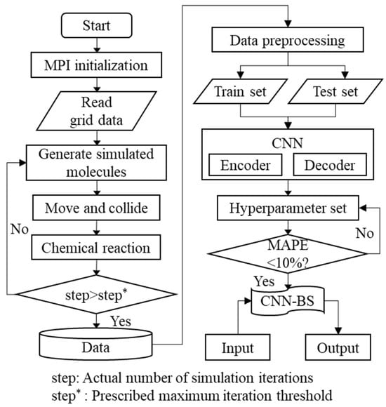
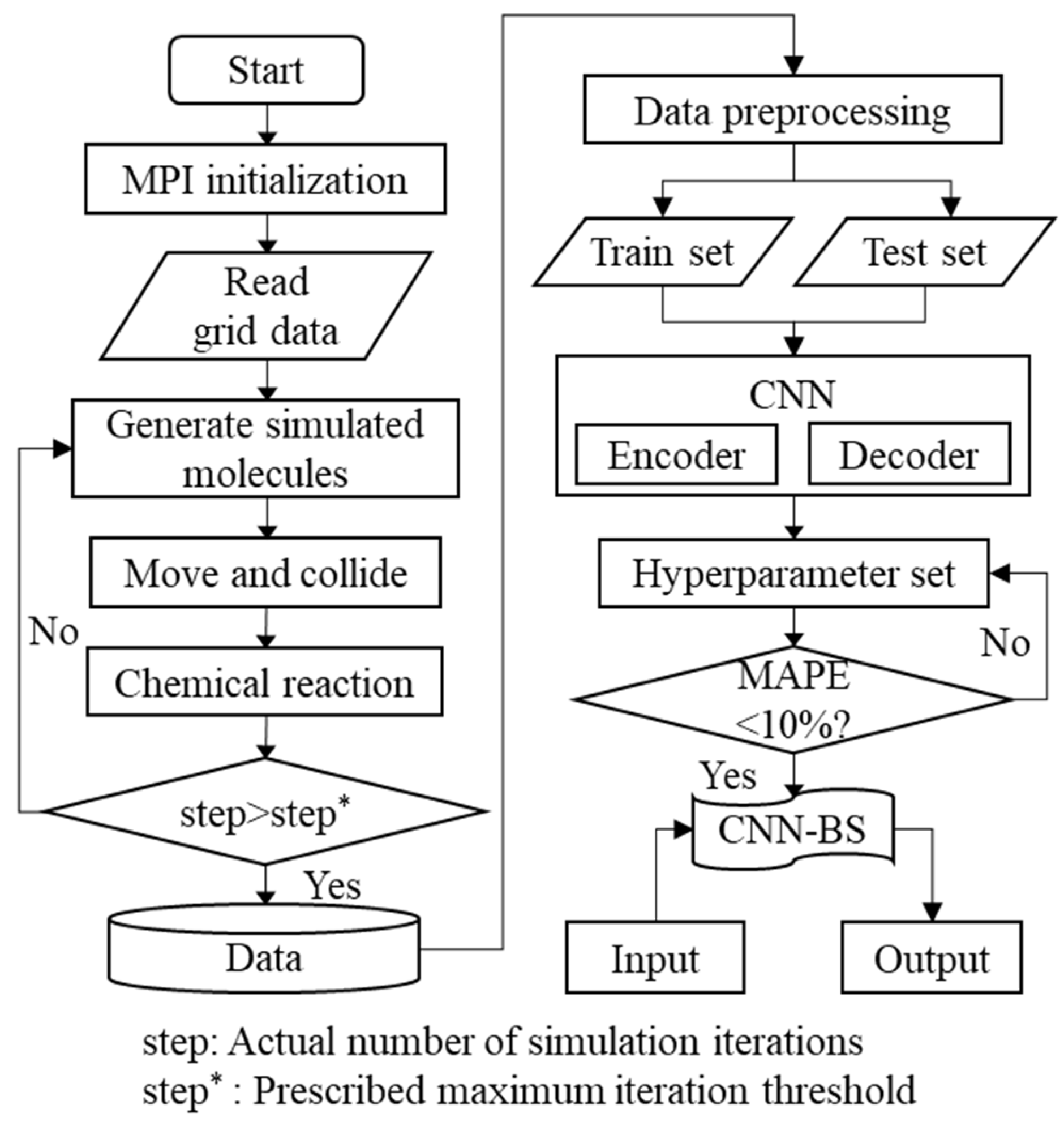
The procedure for constructing the CNN-BS model, as shown in Figure 4, comprises four main stages: MPI parallel computation setup, DSMC numerical simulation, CNN training, and model prediction. First, the MPI parallel environment was configured for parameter synchronization, grid loading and distribution. Subsequently, an iterative solution was obtained for the molecular motion, collision, and chemical reaction processes using the DSMC method. Subsequently, the flow-field data were output once the flow field converged and reached a statistical steady state. Next, data pretreatment was conducted on the obtained flow-field results. Thereafter, a CNN was constructed and optimized via supervised learning, and a surrogate model with a prediction error of less than 10% was obtained after training was completed. Consequently, the trained model efficiently predicted the corresponding flow-field distributions from the input flight parameters.
Figure 4.
Overall workflow for establishing the CNN-BS surrogate model.
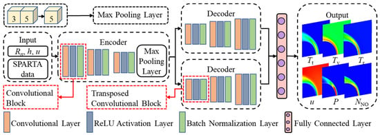
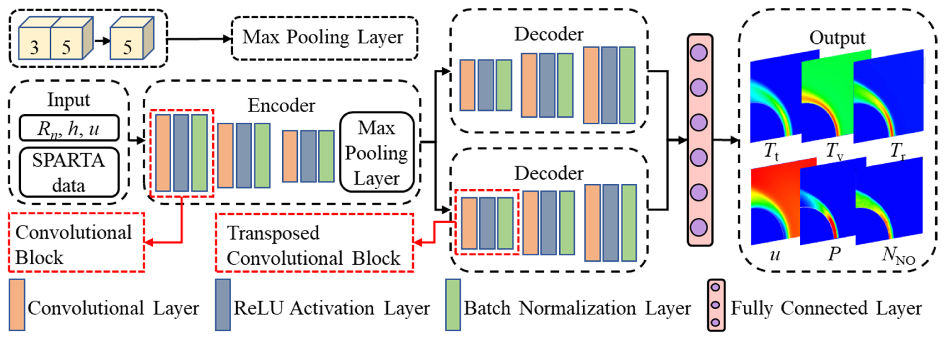
An encoder–decoder architecture was adopted in the CNN-BS model, which comprised a single encoder, two parallel decoders, and a fully connected layer, as illustrated in Figure 5. A parallel decoder structure [39] was introduced to manage the high dimensionality of the output data and to expand the network representation capacity. Based on a shared feature vector, the two decoders reconstructed different flow-field physical quantities separately, thereby effectively improving the reconstruction quality of complex flow fields.
Figure 5.
Architecture of the CNN-BS model.
The network input dimension was set to [3, 1, 1]. The encoder comprised three convolutional blocks, with kernel sizes of 3 × 1, 1 × 3, and 3 × 3. All convolutional layers were equipped with 64 filters, and same padding was applied to preserve the feature map size. Each convolutional layer was followed by a ReLU activation layer and a batch normalization layer. Longitudinal and transverse convolutions were first applied to extract feature correlations along the row and column directions separately, thereby achieving multidimensional feature fusion and mining two-dimensional spatial information. Finally, a 2 × 1 max-pooling layer with the same padding was utilized at the end of the encoder for downsampling, which reduced the dimensionality along the row direction and compressed the feature maps while preserving valid column-wise information.
The low-dimensional feature vectors output by the encoder were separately fed into the two decoding branches. Each branch contained three cascaded deconvolutional blocks with kernel sizes of 1 × 1, 3 × 1, and 1 × 1, and filter numbers of 64, 32, and 32, respectively. The same padding strategy was adopted in all deconvolutional layers to maintain consistent feature map dimensions. Each deconvolutional block was sequentially composed of a deconvolutional layer, a ReLU activation layer, and a batch normalization layer. This structure preserved feature representation capability while effectively alleviating the vanishing gradient problem. Through layer-by-layer deconvolution and upsampling, the feature maps were gradually restored to their original size. Subsequently, the feature maps were mapped to the flow-field parameters via the fully connected layer, completing the flow-field reconstruction.
4. Results and Discussion
4.1. Hyperparameter Tuning
Large discrepancies in terms of the order of magnitude existed among various physical quantities, including the temperature fields Tt, Tv, and Tr, the velocity field u, the pressure field P, and the species field NNO. These variables were categorized into six independent training tasks to reduce their adverse effects on the stability of model training. Key hyperparameters, such as the initial learning rate and batch size, were set during training. The maximum number of training epochs was dynamically adjusted based on the decreasing trend of the training loss. Similarly, the learning-rate decay period was modified based on the convergence state of the model. Additionally, an early-stopping mechanism was adopted to prevent overfitting during model training. Specifically, training was terminated when the loss-function value on the test set did not decrease after 30 consecutive iterations.
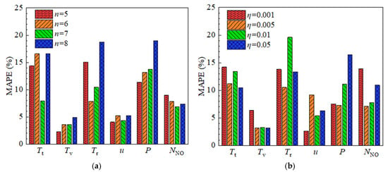
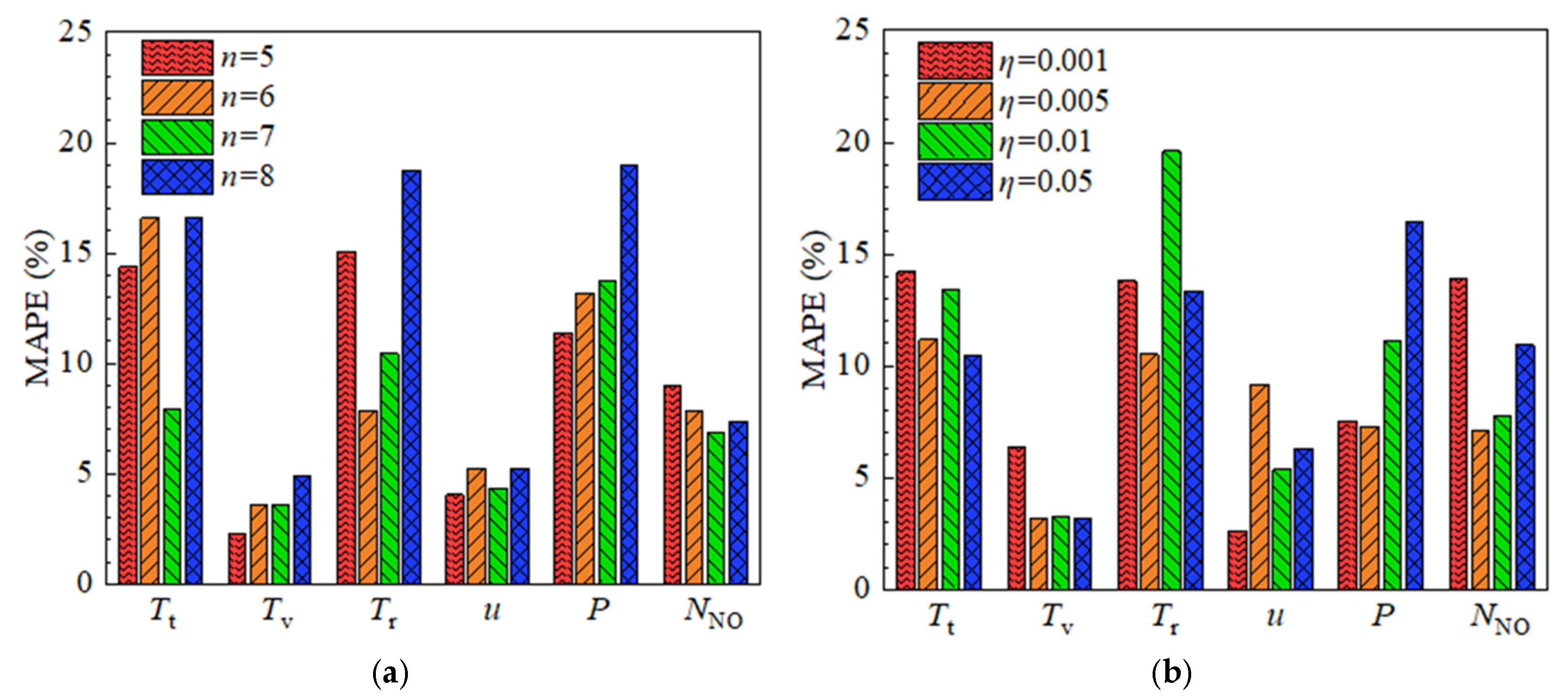
The initial learning rate determines the update step size of the model parameters in each iteration, which directly affects the convergence speed and training stability. To determine a suitable initial learning rate, the effects of different initial learning rates on the model prediction accuracy were compared under a fixed learning rate decay factor of 0.05 and a batch size of 8. The results are shown in Figure 6a. Different physical fields exhibited different sensitivities to the initial learning rate η, among which fluctuations in Tr and P were the most significant. Additionally, the u and P performed better at relatively low initial learning rates, whereas Tv achieved a smaller error at higher initial learning rates. NNO obtained the lowest error at η = 0.005, and the prediction accuracy of Tt showed no significant difference between η = 0.005 and η = 0.05.
Figure 6.
MAPE under different hyperparameter configurations: (a) different initial learning rates and (b) different batch sizes.
The batch size determines the number of samples used for gradient calculation before each parameter update, which affects the training dynamics and generalizability of the model. The appropriate batch-size configuration for the present problem was investigated by analyzing the effect of batch size on the model prediction accuracy. Comparisons were performed under an initial learning rate of 0.005 and a learning rate decay factor of 0.05, and the results are presented in Figure 6b. When the batch size n = 7, the MAPE for all variables was generally low. In particular, the model exhibited outstanding performance in terms of Tv, u, and NNO, with optimal accuracy and stability. Tr and Tt were the most sensitive to variations in the batch size. The MAPE values of Tv and u were below 10% for all batch sizes, thus indicating the overall high prediction accuracy of the model for these two variables.
The hyperparameters were further adjusted for training tasks with relatively large errors to reduce prediction bias and improve model robustness. The prediction errors of the final CNN-BS model on the test set are listed in Table 2. The MAPE of all training tasks was below 8% and the R2 exceeded 0.9. These results reflect the high prediction accuracy and satisfactory generalizability of the model.
Table 2.
Prediction errors on the test set.
4.2. Prediction-Performance Evaluation
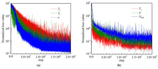
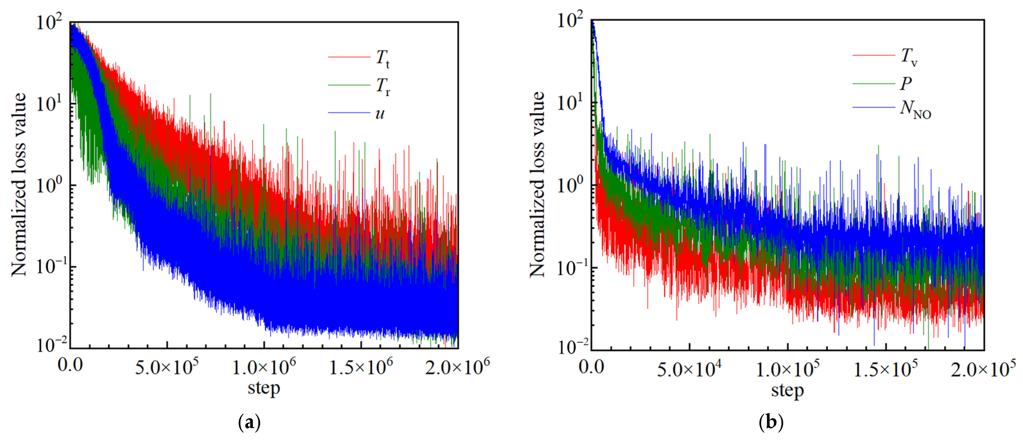
By optimizing the hyperparameter configuration for each training task, the MAPE was effectively reduced. Figure 7 presents the loss-function curves of all the training tasks during training. The horizontal and vertical axes represent the number of iterations and the normalized loss value, respectively. The results show that the loss-function curves of all tasks exhibited a clear downward trend and eventually converged. Specifically, the loss values of Tt, Tr, and u stabilized after approximately 1.0 × 10⁶ iterations. By contrast, Tv, P, and NNO achieved relatively high convergence rates and reached a convergent state after approximately 1.0 × 10⁵ iterations.
Figure 7.
Training loss curves of the CNN-BS model for different flow-field physical quantities: (a) Tt, Tr, and u; (b) Tv, P, and NNO.
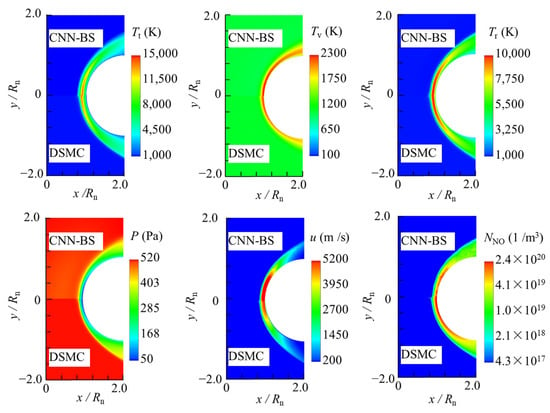
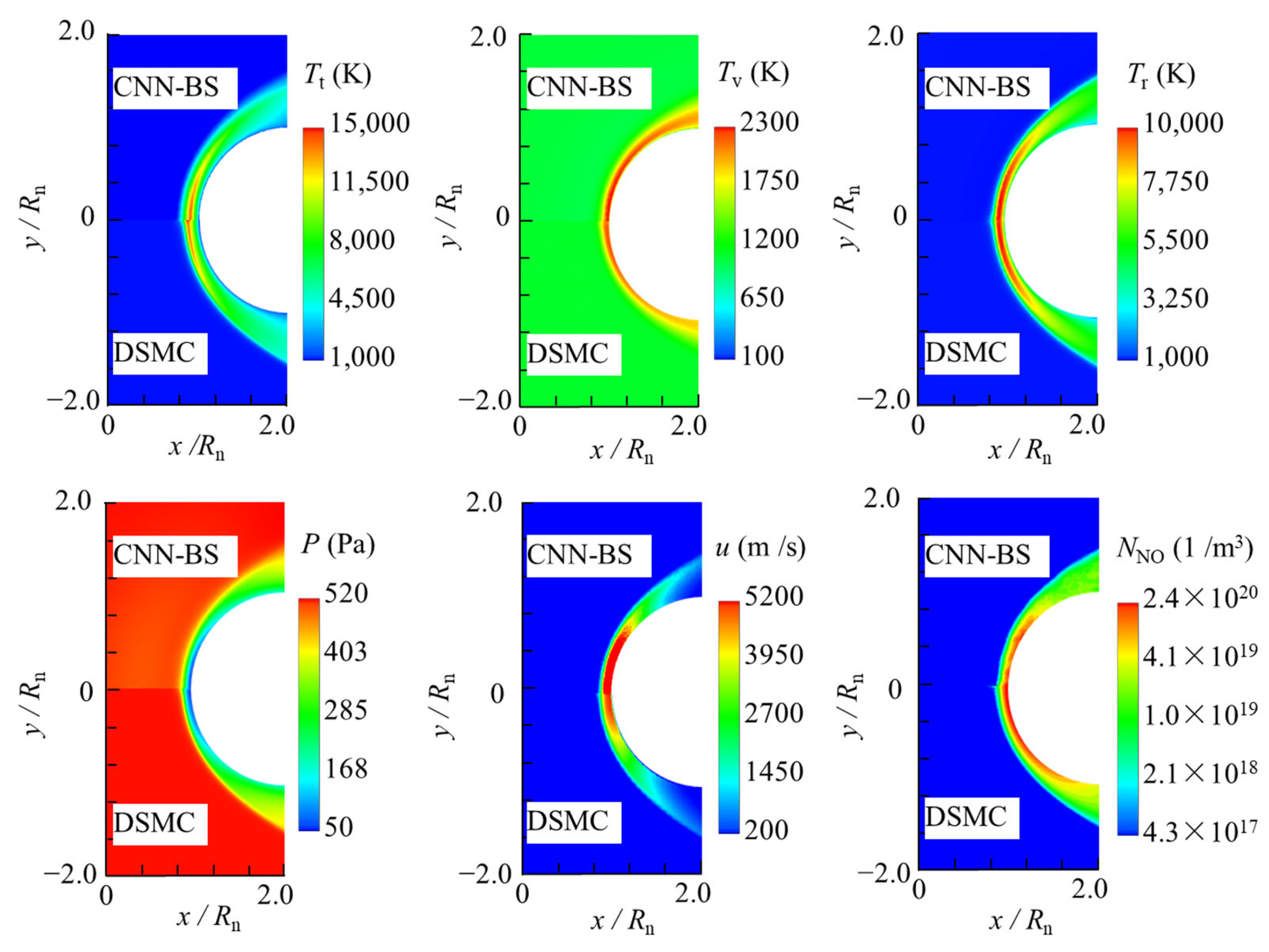
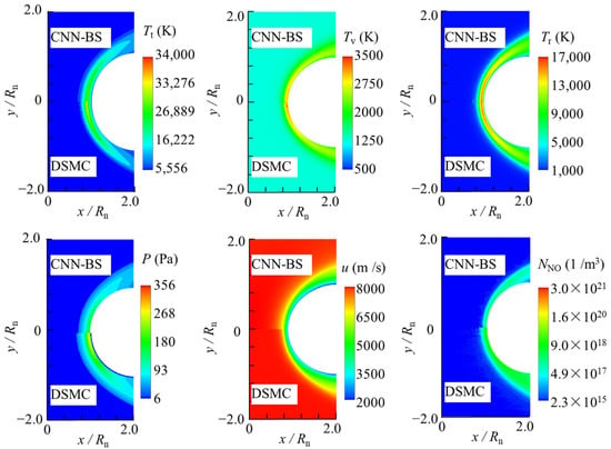
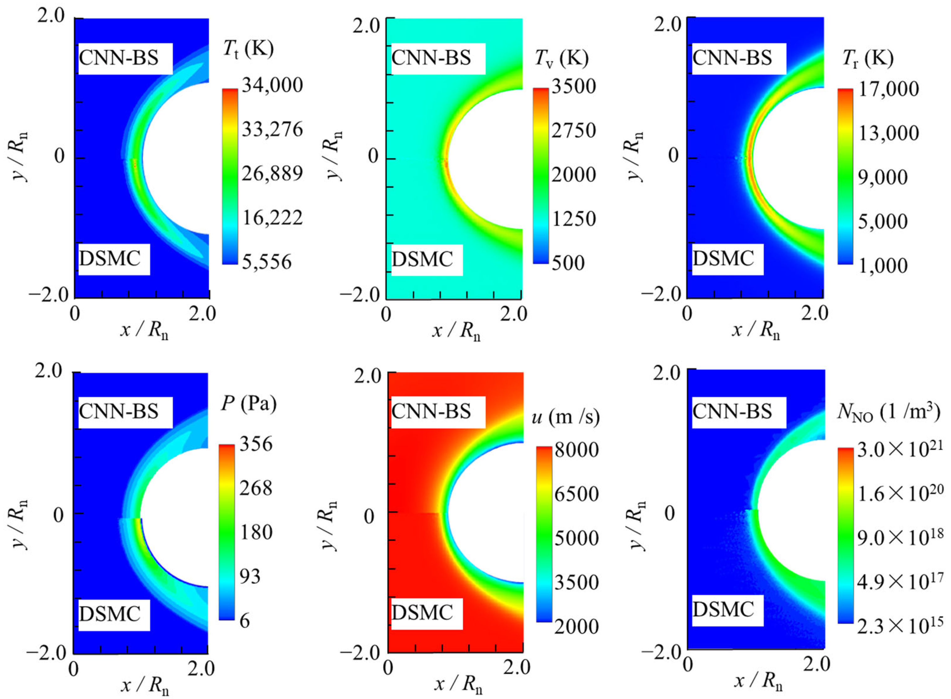
Figure 8 and Figure 9 show a comparison of the prediction results of the CNN-BS model with the DSMC numerical simulation results for Case 16 and Case 41. The input parameters were Rn = 0.4 m, h = 80 km, and u = 5500 m/s for Case 16, and Rn = 0.85 m, h = 90 km, u = 9500 m/s for Case 41. Certain differences were observed in the prediction accuracy of each physical quantity. Specifically, Tv and u achieved the highest prediction accuracies, with MAPE values below 2.7%. The predicted values of Tt and P were slightly higher than the reference values, whereas those of Tr and NNO were slightly lower than the reference values. However, the maximum MAPE remained within 8%.
Figure 8.
Comparison of flow-field contours between DSMC simulation and CNN-BS prediction for Case 16.
Figure 9.
Comparison of flow-field contours between DSMC simulation and CNN-BS prediction for Case 41.
4.3. Analysis of Flow-Field Parameter Effects Based on Surrogate Model
The LHS method was adopted in this study to systematically evaluate the prediction performance of the CNN-BS model. Fifty test cases were sampled in the parameter space spanned by the flight altitude h and velocity u. Subsequently, the trained CNN-BS model was used to predict the bow-shock reactive flow fields for each case.
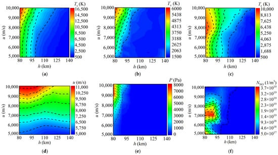
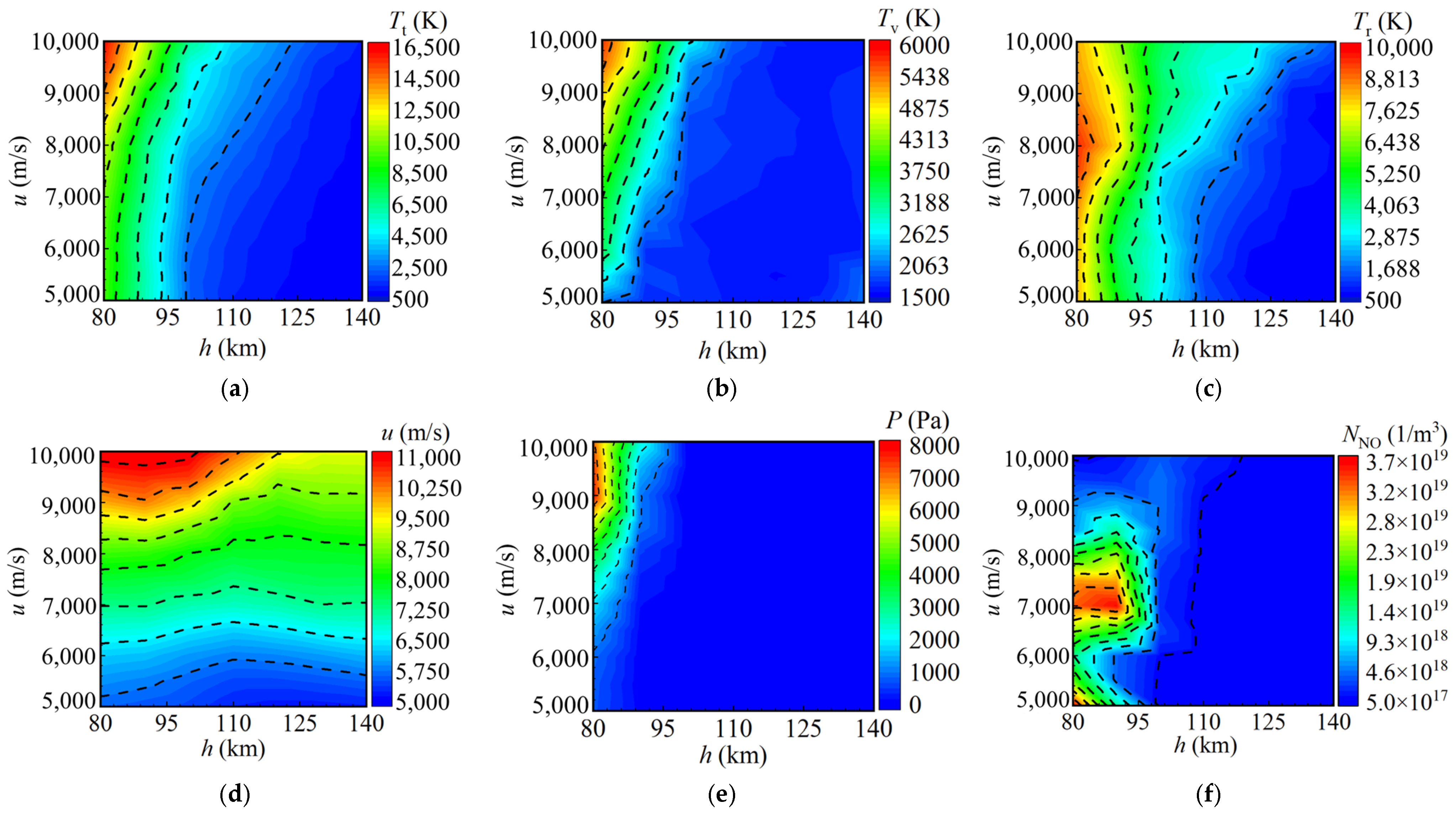
Figure 10a–c present the peak distributions of the translational, rotational, and vibrational temperatures at different flight altitudes and velocities when the nose radius was 0.1 m. The results show that both the translational and vibrational temperatures reached their maximum values at an altitude of 80 km and a velocity of 10,000 m/s. At a fixed altitude, the peak translational and vibrational temperatures increased with the velocity. However, the peak rotational temperature showed a different pattern, i.e., initially increasing and then decreasing. When the velocity was fixed, the peak translational and vibrational temperatures decreased with increasing altitude. These differences arise from non-equilibrium relaxation of internal energy. Translational energy exchange is rapid, causing the translational temperature to surge after shock compression and remain significantly higher than the rotational and vibrational temperatures. In the rarefied high-altitude flow, the low collision frequency delays vibrational energy transfer, so the vibrational temperature deviates noticeably from the translational temperature in both variation and peak location, while its overall minimum remains higher.
Figure 10.
Peak distributions of flow-field parameters at Rn = 0.1 m under different flight altitudes and velocities: (a) Tt; (b) Tv; (c) Tr; (d) u; (e) P; (f) NNO.
Figure 10d–f show the peak distributions of the velocity, pressure, and NO number density at different flight altitudes and velocities, respectively. The results indicate that the peak values of u and P reached their maximum at h = 80 km and u = 10,000 m/s. The distribution trends of the peaks were consistent with those of Tt and Tv. By contrast, the peak value of NNO appeared at u ≈ 7000 m/s. The peak NNO showed a downward trend when the velocity deviated from this value. From the perspective of the altitude effect, NNO remained at a high level within the range of 80–100 km and decreased significantly beyond this range. From reaction kinetics, insufficient shock compression at lower velocities leads to slow NO production. Above 7000 m/s, NO declines as residence time shortens, reverse reactions intensify, and weak ionization consumes neutral NO. At higher altitudes, extreme rarefaction suppresses chemical reactions, reducing the NO number density.
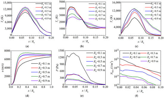
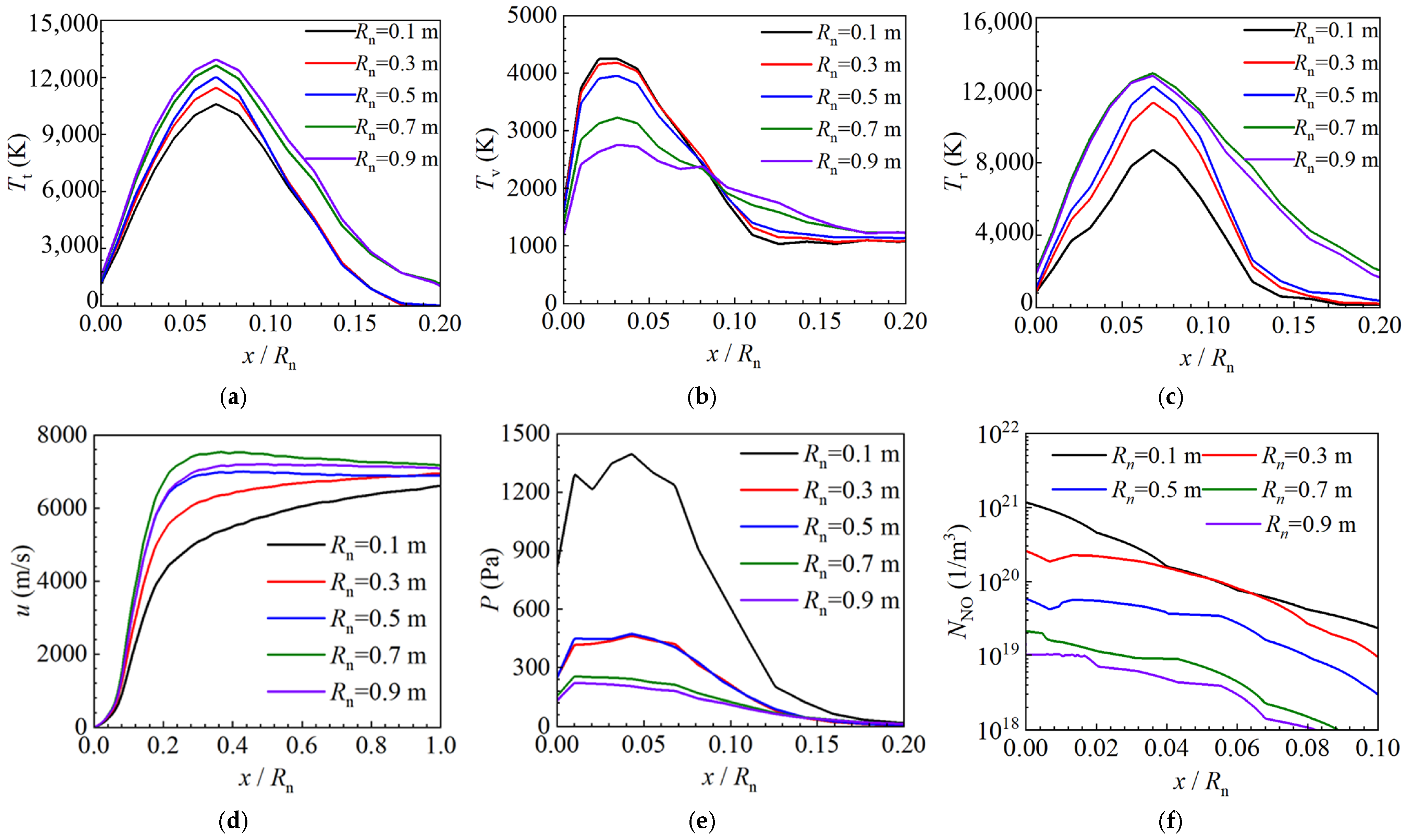
Figure 11a–f present the stagnation line flow-field parameter distributions corresponding to different blunt-body nose radii at an altitude of 80 km and a velocity of 7000 m/s. A change in the nose radius alters the curvature of the windward surface of the blunt body, thereby modifying the compression state of the incoming flow. A larger nose radius weakens the local compression of the flow, which reduces the vibrational temperature and pressure. Meanwhile, the coupling between molecular thermal motion and macroscopic flow is enhanced, causing the translational temperature, rotational temperature, and flow velocity to increase accordingly. Along the stagnation line, both temperature and pressure first increase and then decrease with increasing distance from the wall. In addition, a larger nose radius leads to a gentler near-wall velocity gradient and a weaker flow deceleration effect ahead of the blunt body.
Figure 11.
Flow-field parameter profiles along stagnation line for different nose radii at h = 80 km and u = 7000 m/s: (a) Tt; (b) Tv; (c) Tr; (d) u; (e) P; (f) NNO.
4.4. Computational Efficiency Evaluation
We compare the CPU runtime of DSMC simulations and CNN-BS predictions. The DSMC simulations were performed on a VMware virtual machine running Ubuntu 22.04, equipped with an Intel i7-13700K processor and allocated 4 CPU cores, while the CNN model inference was conducted on a Windows 11 system using the Matlab R2022a platform. All computations were carried out solely on the CPU without GPU acceleration. The DSMC numerical simulations for all 100 sample cases took approximately 2320 h in total. After hyperparameter tuning, the one-time offline training of the CNN model was completed within one day, and the aforementioned dataset generation and network training represented a one-time upfront fixed cost. Therefore, the speedup reported here corresponds exclusively to the single online prediction of previously unseen operating conditions after model training convergence, excluding these upfront costs. As shown in Table 3, a single DSMC simulation required approximately 20 h on average, whereas the CNN-BS model required only 0.5 s per prediction, achieving a speedup of approximately 144,000 times and an improvement in computational efficiency of approximately five orders of magnitude. This offers a significant advantage in engineering scenarios that require rapid batch predictions for a large number of operating conditions.
Table 3.
Comparison of computation time.
5. Conclusions
In this study, a rapid prediction model (CNN-BS) for the bow-shock reactive flow field around a blunt body in a high-altitude rarefied flow regime was established based on a CNN. The nose radius, flight altitude, and flight velocity were adopted as the input parameters. The prediction performance of the CNN-BS model was evaluated, and the main conclusions are as follows:
(1) The CNN-BS model accurately predicted the translational temperature, rotational temperature, vibrational temperature, velocity, pressure, and NO number density of bow shock. The prediction results were consistent with the numerical-simulation results.
(2) The CNN-BS model exhibited good reconstruction capability for multiple physical fields and high prediction stability. For all output parameters on the test set, the MAPE was below 8%, and the R2 exceeded 0.9.
(3) The average single prediction time of the CNN-BS model was approximately 0.5 s. Compared with the classical DSMC method, the proposed model exhibited a higher computational efficiency by five orders of magnitude. The model can realize batch computation and real-time prediction, thus providing an efficient tool for the radiation-noise evaluation of seekers and thermal-protection design.
Although the CNN-BS model has high accuracy and computational efficiency, it has some limitations. It is only applicable to axisymmetric flows around single blunt bodies within the given parameter range of altitude and Mach number, and merely predicts NO number density and basic flow parameters. In future research, we will adopt alternative network architectures to adapt the model for 3D flows and complex geometries. We will also expand the parameter range of training data and upgrade the network to realize multi-species and high-order flow characteristic predictions. These efforts will broaden the model’s application scope.
Author Contributions
Conceptualization, Y.W. and X.S.; methodology, Y.W.; software, Y.W.; validation, Y.W. and X.S.; formal analysis, X.M.; investigation, Y.S.; resources, Y.S.; data curation, Y.S.; writing—original draft preparation, Y.W.; writing—review and editing, Q.N.; visualization, Y.W.; supervision, Q.N.; funding acquisition, Q.N. All authors have read and agreed to the published version of the manuscript.
Funding
This research was funded by the National Natural Science Foundation of China, grant numbers 52576099 and U22B2045, and the Fundamental Research Program of Shanxi Province, grant number 202403021211078.
Data Availability Statement
The data that support the findings of this study are available from the corresponding author upon reasonable request.
Conflicts of Interest
The authors declare no conflicts of interest.
Abbreviations
The following abbreviations are used in this manuscript:
| DSMC | Direct Simulation Monte Carlo |
| CNN | Convolutional Neural Network |
| CNN-BS | Convolutional Neural Network–Bow Shock |
| BSUV | Bow Shock UltraViolet |
| NO | Nitric Oxide |
| VSS | Variable Soft Sphere |
| TCE | Total Collision Energy |
| ReLU | Rectified Linear Unit |
| MAPE | Mean Absolute Percentage Error |
| LHS | Latin Hypercube Sampling |
| MPI | Message Passing Interface |
References
- Li, J.; Zhu, Y.; Luo, X. On type VI–V transition in hypersonic double-wedge flows with thermo-chemical non-equilibrium effects. Phys. Fluids 2014, 26, 86104. [Google Scholar] [CrossRef] [Scilit]
- Tang, W.-X.; Ding, T.; Li, D.-X.; Zhang, C.-H.; Li, P. Study of High-Temperature Air Radiation Spectrum Under High-Speed Shock Wave. Spectrosc. Spectr. Anal. 2024, 44, 2739–2744. [Google Scholar] [CrossRef]
- Levin, D.A.; Caveny, L.H.; Mann, D.M. Ultraviolet emissions quantified by rocket payloads. In Proceedings of the Ultraviolet Technology IV; SPIE: Bellingham, WA, USA, 1993; pp. 388–399. [Google Scholar] [CrossRef] [Scilit]
- Votta, R.; Schettino, A.; Bonfiglioli, A. Hypersonic high altitude aerothermodynamics of a space re-entry vehicle. Aerosp. Sci. Technol. 2013, 25, 253–265. [Google Scholar] [CrossRef] [Scilit]
- Erdman, P.W.; Zipf, E.C.; Espy, P.; Howlett, C.; Levin, D.A.; Loda, R.; Collins, R.J.; Candler, G.V. Flight measurements of low-velocity bow shock ultraviolet radiation. J. Thermophys. Heat Transf. 1993, 7, 37–41. [Google Scholar] [CrossRef] [Scilit] [PubMed]
- Erdman, P.W.; Zipf, E.C.; Espy, P.; Howlett, C.L.; Levin, D.A.; Collins, R.J.; Candler, G.V. Measurements of ultraviolet radiation from a 5-km/s bow shock. J. Thermophys. Heat Transf. 1994, 8, 441–446. [Google Scholar] [CrossRef] [Scilit] [PubMed]
- Surzhikov, S.; Kozlov, P. Nonequilibrium radiation NO in shocked air. In Proceedings of the 55th AIAA Aerospace Sciences Meeting, Grapevine, TX, USA, 9–13 January 2017; p. 0157. [Google Scholar] [CrossRef] [Scilit]
- Boyd, I.D. Conservative species weighting scheme for the direct simulation Monte Carlo method. J. Thermophys. Heat Transf. 1996, 10, 579–585. [Google Scholar] [CrossRef] [Scilit] [PubMed]
- Boyd, I.; Phillips, W.; Levin, D.; Boyd, I.; Phillips, W.; Levin, D. Sensitivity studies for prediction of ultra-violet radiation in nonequilibrium hypersonic bow-shock waves. In Proceedings of the 35th Aerospace Sciences Meeting and Exhibit, Reno, NV, USA, 6–9 January 1997; p. 131. [Google Scholar] [CrossRef] [Scilit]
- Levin, D.A.; Candler, G.V.; Collins, R.J.; Erdman, P.W.; Zipf, E.C.; Howlett, L.C. Examination of theory for bow shock ultraviolet rocket experiments. II. J. Thermophys. Heat Transf. 1994, 8, 447–452. [Google Scholar] [CrossRef] [Scilit] [PubMed]
- Karpuzcu, I.T.; Thirani, S.; Levin, D.A.; Andrienko, D. Nitric Oxide Infrared Radiation Modeling from a Hypersonic Flow. In Proceedings of the AIAA AVIATION 2022 Forum, Chicago, IL, USA, 27 June–1 July 2022; p. 3501. [Google Scholar] [CrossRef]
- Sun, X.; Wang, Y.; Liu, S. Modeling and Study of UV Radiation Characteristics in the Surrounding Environment of Hypersonic Vehicles. Int. J. Aeronaut. Space Sci. 2026, 27, 2130–2149. [Google Scholar] [CrossRef] [Scilit]
- Toussaint, D.; Braeunig, J.-P.; Baranger, C.; Noubel, H.; Lago, V. Numerical investigation of the influence of the rarefaction degree on a waverider aerodynamic performances in super-/hypersonic regimes. In Proceedings of the AIAA AVIATION 2023 Forum, San Diego, CA, USA, 12–16 June 2023; p. 3849. [Google Scholar] [CrossRef] [Scilit]
- Tumuklu, O.; Hanquist, K.M. Hypersonic turbulence wake modeling from rarefied to continuum regimes. In Proceedings of the AIP Conference Proceedings; AIP Publishing LLC: Melville, NY, USA, 2024; p. 080013. [Google Scholar] [CrossRef] [Scilit]
- Cimini, M.; Pizzarelli, M.; Bernardini, M. Aerothermodynamic analysis of high-altitude space launcher with direct-simulation Monte Carlo method. AIAA J. 2019, 57, 2534–2543. [Google Scholar] [CrossRef] [Scilit]
- Shi, H.; Bai, L.; Zhou, J.; Li, Y.; Zhang, L. The impact of chemical non-equilibrium models on the ultraviolet spectral radiation characteristics of shock layers. In Proceedings of the Second Conference on Space, Atmosphere, Marine, and Environmental Optics (SAME 2024), Hangzhou, China, 8–10 April 2024; pp. 102–107. [Google Scholar] [CrossRef] [Scilit]
- Candler, G. On the computation of shock shapes in nonequilibrium hypersonic flows. In Proceedings of the 27th Aerospace Sciences Meeting, Reno, NV, USA, 9–12 January 1989; p. 312. [Google Scholar] [CrossRef] [Scilit]
- Niu, Q.; Yuan, Z.; Dong, S.; Tan, H. Assessment of nonequilibrium air-chemistry models on species formation in hypersonic shock layer. Int. J. Heat Mass Transf. 2018, 127, 703–716. [Google Scholar] [CrossRef] [Scilit]
- Li, D.; Sun, B.; Dai, C.; Chen, X.; Zhang, X.; Man, Y. Influences of thermochemical non-equilibrium effects on Type III shock/shock interaction at Mach 10. Acta Astronaut. 2024, 214, 553–566. [Google Scholar] [CrossRef] [Scilit]
- Bird, G.A. Molecular Gas Dynamics and the Direct Simulation of Gas Flows; Oxford University Press: Oxford, UK, 1994. [Google Scholar] [CrossRef] [Scilit]
- Gupta, V.K. Mathematical Modeling of Rarefied Gas Mixtures. Ph.D. Thesis, Technische Hochschule, Aachen, Germany, 2015. [Google Scholar]
- Scanlon, T.; Roohi, E.; White, C.; Darbandi, M.; Reese, J. An open source, parallel DSMC code for rarefied gas flows in arbitrary geometries. Comput. Fluids 2010, 39, 2078–2089. [Google Scholar] [CrossRef] [Scilit]
- Norman, P.; Valentini, P.; Schwartzentruber, T. GPU-accelerated classical trajectory calculation direct simulation Monte Carlo applied to shock waves. J. Comput. Phys. 2013, 247, 153–167. [Google Scholar] [CrossRef] [Scilit]
- Tumuklu, O.; Levin, D.; Theofilis, V. Assessment of degree of steadiness in boundary layer shock-interaction flows. AIAA Pap. 2017, 1614, 2017. [Google Scholar]
- Li, R.; Song, B.; Chen, Y.; Jin, X.; Zhou, D.; Han, Z.; Chen, W.-L.; Cao, Y. Deep learning reconstruction of high-Reynolds-number turbulent flow field around a cylinder based on limited sensors. Ocean Eng. 2024, 304, 117857. [Google Scholar] [CrossRef] [Scilit]
- Jin, X.; Cheng, P.; Chen, W.-L.; Li, H. Prediction model of velocity field around circular cylinder over various Reynolds numbers by fusion convolutional neural networks based on pressure on the cylinder. Phys. Fluids 2018, 30. [Google Scholar] [CrossRef] [Scilit]
- Hasegawa, K.; Fukami, K.; Murata, T.; Fukagata, K. Machine-learning-based reduced-order modeling for unsteady flows around bluff bodies of various shapes. Theor. Comput. Fluid Dyn. 2020, 34, 367–383. [Google Scholar] [CrossRef] [Scilit]
- Cai, G.; Zhang, B.; Liu, L.; Weng, H.; Wang, W.; He, B. Fast vacuum plume prediction using a convolutional neural networks-based direct simulation Monte Carlo method. Aerosp. Sci. Technol. 2022, 129, 107852. [Google Scholar] [CrossRef] [Scilit]
- Roohi, E.; Shoja-Sani, A. Data-driven surrogate modeling of DSMC solutions using deep neural networks. Aerosp. Sci. Technol. 2025, 168, 110785. [Google Scholar] [CrossRef] [Scilit]
- Hervella, Á.S.; Rouco, J.; Novo, J.; Ortega, M. Multi-adaptive optimization for multi-task learning with deep neural networks. Neural Netw. 2024, 170, 254–265. [Google Scholar] [CrossRef] [Scilit] [PubMed]
- Jia, Y.; Li, Z.; Zhang, C.; Ma, H.; Hao, J.; Wen, C.-Y. Prediction of shock and boundary layer interaction in supersonic/hypersonic flow over a compression ramp using deep neural networks. Aerosp. Sci. Technol. 2025, 110976. [Google Scholar] [CrossRef] [Scilit]
- Roohi, E.; Mahdavi, A. Analysis of the rarefied flow at micro-step using a DeepONet surrogate model with a physics-guided zonal loss function. Microfluid. Nanofluidics 2026, 30, 44. [Google Scholar]
- Plimpton, S.J.; Moore, S.; Borner, A.; Stagg, A.; Koehler, T.; Torczynski, J.; Gallis, M. Direct simulation Monte Carlo on petaflop supercomputers and beyond. Phys. Fluids 2019, 31, 086101. [Google Scholar] [CrossRef] [Scilit]
- Gimelshein, S.F.; Wysong, I.J. Bird’s total collision energy model: 4 decades and going strong. Phys. Fluids 2019, 31, 076101. [Google Scholar] [CrossRef] [Scilit]
- Hwang, W.; Lee, D.; Shin, J.; Cho, K.; Choi, S. Aerodynamic flow analysis using conditional convolutional autoencoder in various flow conditions and application to CFD-based design optimization. Adv. Aerodyn. 2025, 7, 12. [Google Scholar] [CrossRef] [Scilit]
- Xuan, A.; Shen, L. Reconstruction of three-dimensional turbulent flow structures using surface measurements for free-surface flows based on a convolutional neural network. J. Fluid Mech. 2023, 959, A34. [Google Scholar] [CrossRef] [Scilit]
- De Myttenaere, A.; Golden, B.; Le Grand, B.; Rossi, F. Mean absolute percentage error for regression models. Neurocomputing 2016, 192, 38–48. [Google Scholar] [CrossRef] [Scilit]
- Wu, S.; Li, G.; Deng, L.; Liu, L.; Wu, D.; Xie, Y.; Shi, L. L1-norm batch normalization for efficient training of deep neural networks. IEEE Trans. Neural Netw. Learn. Syst. 2018, 30, 2043–2051. [Google Scholar] [CrossRef] [Scilit] [PubMed]
- Sofos, F.; Drikakis, D.; Kokkinakis, I.W.; Spottswood, S.M. Convolutional neural networks for compressible turbulent flow reconstruction. Phys. Fluids 2023, 35, 116120. [Google Scholar] [CrossRef] [Scilit]

Disclaimer/Publisher’s Note: The statements, opinions and data contained in all publications are solely those of the individual author(s) and contributor(s) and not of MDPI and/or the editor(s). MDPI and/or the editor(s) disclaim responsibility for any injury to people or property resulting from any ideas, methods, instructions or products referred to in the content. |
© 2026 by the authors. Licensee MDPI, Basel, Switzerland. This article is an open access article distributed under the terms and conditions of the Creative Commons Attribution (CC BY) license.