


Abstract
Shock buffet is one of the critical issues affecting the aerodynamic performance, flight quality, and flight safety of large aircraft. To overcome the limitations of traditional experimental measurement methods, such as insufficient capability in capturing flow features and high cost, an integrated experimental system tailored for extreme cryogenic and high-Reynolds-number conditions is developed based on the conventional tuft technique. This system comprises “preparation of low-flow-disturbance fluorescent mini-tufts, high-efficiency large-area tuft taping, automatic generation of digital streamline, and flow topology analysis”. Furthermore, a technique for assessing the transonic shock buffet onset using dynamic flow visualization with fluorescent mini-tufts is proposed. This paper takes a typical supercritical airfoil as the research object. First, through high-precision numerical simulations, it reveals that low-energy, unstable boundary-layer separation is the core driving force for the development and maintenance of shock buffet, and that flow separation characteristics serve as an important basis for determining the shock buffet onset. Subsequently, experimental validation is conducted in a 0.3 m high-Reynolds-number transonic wind tunnel. Using a dual-excitation-band composite light source, simultaneous measurements of pressure-sensitive paint (PSP) and fluorescent mini-tuft patterns are realized. The experimental results show that under extreme conditions, characterized by a wide total temperature range of 110 K to 280 K and strong scouring at Mach numbers from 0.6 to 0.9, the fluorescent mini-tufts (approximately 0.05 mm in diameter) exhibit excellent flow-following capability without any detachment. The digitized flow patterns of the fluorescent mini-tufts, obtained via computer image recognition algorithms, clearly reveal the location and area of boundary-layer separation. The trends show good agreement with the cryogenic PSP results, providing an important reference for determining the shock buffet onset.
1. Introduction
In the process of the aerodynamic design and optimization of large aircraft, shock buffet has always been a key concern for aircraft designers, and understanding its buffet onset is crucial for enhancing aerodynamic performance and flight safety [1]. Giannelis et al. comprehensively reviewed recent developments in transonic shock buffet, emphasizing the complexity of its underlying physics and the challenges in predicting buffet onset [2]. Research indicates that shock buffet is a complex aerodynamic flow phenomenon characterized by periodic coupling variations among shock wave location, shock intensity, and the boundary-layer separation region [3]; as summarized by Lee, this self-sustained shock oscillation involves a feedback loop between the shock motion and the disturbances propagating in the separated flow and wake [4]. More recently, Gao and Zhang provided a new perspective from the fluid mode, revealing that the decrease in flow stability in the transonic regime makes the fluid mode a dominant factor in fluid–structure coupling, thereby explaining phenomena such as transonic buzz and frequency lock-in [5]. Once buffet occurs, it can reduce the fatigue life of the aircraft, degrade ride comfort, interfere with the normal operation of the flight control system, and may even cause structural damage [6]. For large aircraft such as civil airliners, the safety margin between the buffet onset and the cruise condition directly determines the success or failure of the design [7].
The core of shock buffet onset assessment lies in determining the critical combinations of key parameters such as buffet onset Mach number and angle of attack. However, the three-dimensional coupling effects, broadband characteristics, and Reynolds-number sensitivity of shock buffet further increase the difficulty of accurate assessment [8]. Current mainstream methods can be divided into two categories: numerical simulation and experimental measurement [9]. Numerical computation provides low-cost, high-efficiency support for buffet mechanism research and full-process design, but its accuracy and reliability are still subject to validation against experimental data due to limitations in physical modeling, computational capability, and turbulence simulation. The steady numerical criterion of “drag coefficient increment of 0.005” proposed by Airbus based on CFD calculations has been widely applied in the A320 series [10]. Although computationally efficient, this criterion neglects the unsteady nature of shock buffet. Subsequent flight tests have revealed a prediction error of up to 0.03 Mach number at high angles of attack, exposing the inherent drawback of steady methods in ignoring unsteady effects. The Darmstadt University of Technology proposed an adaptive mesh method based on hybrid RANS/LES. Although this method reduces grid dependency by 30%, it remains sensitive to the adjustment of turbulence model parameters and exhibits poor adaptability across different aircraft configurations [11]. Gao Chuanqiang et al. investigated typical wings such as the Common Research Model (CRM) using URANS simulations and dynamic mode decomposition (DMD) analysis [12]. They found that transonic buffet on the wing manifests as broadband oscillations under multiple instability modes, capturing that shock wave instabilities occur in both the spanwise and chordwise directions and exhibit low-frequency characteristics. These findings provide guidance for physical modeling, control, and understanding of aeroelastic phenomena associated with buffet. However, the accuracy of the URANS method is limited by the turbulence model, and the deviation in simulating shock/turbulent-boundary-layer interactions can reach an order of magnitude. NASA Langley Research Center employed the Improved Delayed Detached Eddy Simulation (IDDES) method to simulate the buffet characteristics of a supercritical wing [13]. Although this approach captures the coupled oscillation between the shock and the separation region, the computational time for a typical case at Ma = 0.85 and Re = 107 reaches 720 h, making it difficult to meet the demands of rapid engineering iteration. Moreover, the method is highly dependent on grid resolution and turbulence model selection. The compressed sensing DMD algorithm developed by the Massachusetts Institute of Technology improves the efficiency of flow field modal identification by 40%, yet it cannot reflect the continuous evolution of dynamic flow patterns in real time [14,15].
Buffet onset evaluation through experiments typically employs unsteady pressure sensors, accelerometers, strain gauges, and similar devices to obtain characteristic signals, such as surface pressure fluctuations, wingtip acceleration, and wing root bending moment, for determining the buffet onset [16,17]. However, conventional methods suffer from discrete measurement points, leading to the incomplete capture of three-dimensional features such as spanwise shock buffet [18]. Moreover, these methods impose stringent requirements on the precision and sensitivity of the testing instruments, and the consistency among different approaches remains to be improved. In recent years, high-resolution dynamic flow visualization techniques have been increasingly used for buffet onset measurement and mechanism research. Although the fluorescence oil flow method [19] is applicable to high-speed flows and can visualize flow patterns, it suffers from long test turnaround time, high wind tunnel cleaning costs, experience-dependent interpretation, and difficulty in achieving continuous observation of dynamic flow patterns. Modern techniques such as particle image velocimetry (PIV) [20] and laser Doppler velocimetry (LDV) [21] are complex to operate and costly, and their application in large-scale wind tunnel tests has yet to reach maturity. They are also highly susceptible to interference from extreme wind tunnel environments and complex flow fields, leading to issues such as measurement distortion, algorithm failure, insufficient temporal resolution, and complicated data processing. The German Aerospace Center (DLR) has employed high-resolution PIV and unsteady pressure-sensitive paint (PSP) to study shock buffet flow fields [22]. Although these methods can capture fine flow structures, the experimental systems are complex and expensive, and their applicability in extreme test environments, such as cryogenic conditions, requires further improvement. The experimental evaluation of buffet characteristics demands a balance among unsteady dynamics, high-resolution full-field measurement, low cost, and convenience.
To address the above issues, this paper develops a shock buffet onset assessment method based on dynamic flow visualization using fluorescent mini-tufts. The method tracks and visualizes the evolution of the flow field through the dynamic response of fluorescent mini-tufts, captures shock-induced flow separation characteristics, and establishes the relationship between the surface flow pattern and the buffet onset Mach number. Meanwhile, pressure-sensitive paint (PSP) is coated on the model surface. By employing a dual-excitation-band composite light source, high-frequency synchronous measurements of PSP pressure distribution and fluorescent mini-tuft patterns are achieved. Comparative analysis and validation further confirm the reliability of the proposed shock buffet onset assessment method based on dynamic flow patterns of fluorescent mini-tufts.
2. Experimental System
2.1. Model and Wind Tunnel
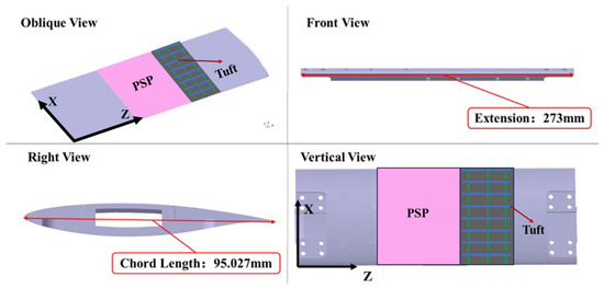
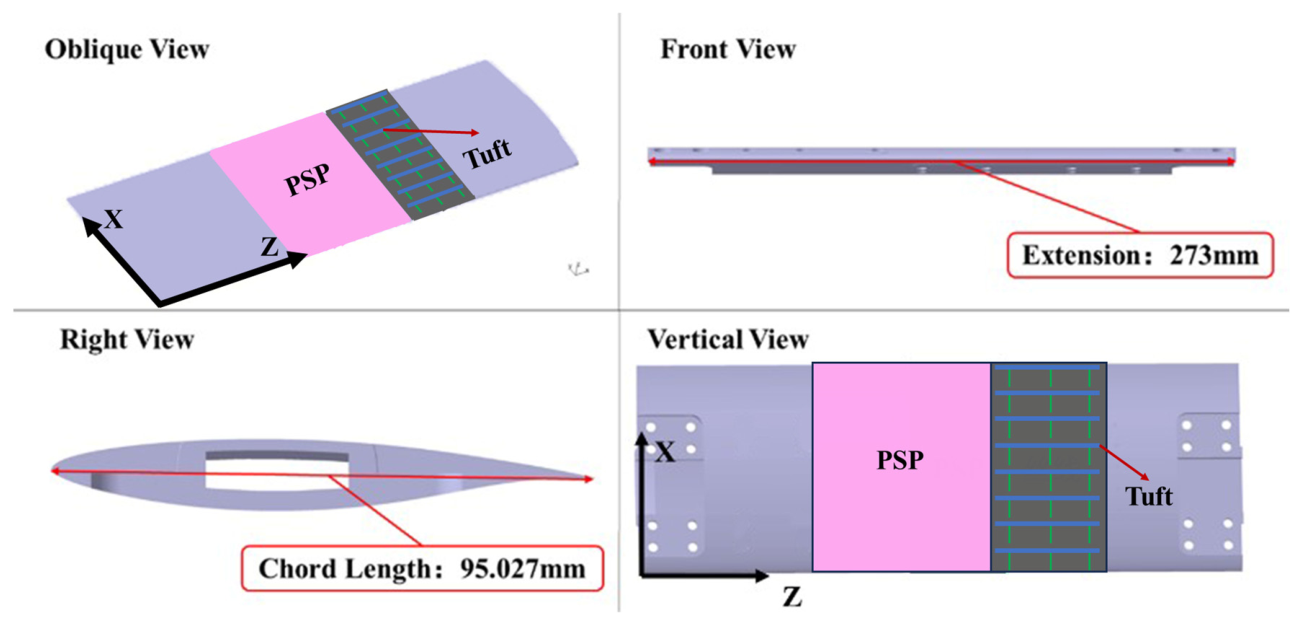
This paper adopts a house-developed supercritical airfoil. The test model has a chord length c = 95.027 mm, a span length b = 273 mm, and a trailing edge thickness of 0.1 mm. Self-developed fluorescent mini-tufts (excitation wavelength 460 nm) and PSP coating (excitation wavelength 400 nm) [23] are arranged at different spanwise positions in the uniform flow region on the upper wing surface. The PSP employed in this study uses Ru(dpp) (tris(4,7-diphenyl-1,10-phenanthroline) ruthenium(II) dichloride) as the luminophore. Its excitation wavelength is 450 nm (blue light), and its emission wavelength is 610 nm (red light). This PSP is suitable for cryogenic and transonic wind tunnel applications within a temperature range of 100 K to 300 K and a pressure range of 10 to 150 kPa, which fully meets the requirements of the unsteady pressure measurements in this study. The angle of attack is varied through a shaft connection to the upper and lower walls of the test section. The model structure and main parameters are shown in Figure 1.
Figure 1.
Test model.
The experiment was conducted in the 0.3 m high-Reynolds-number transonic wind tunnel of the China Aerodynamics Research and Development Center. The test section dimensions are 0.325 m × 0.275 m (width × height). The total temperature ranges from 110 K to 323 K, the total pressure ranges from 0.2 × 10⁵ Pa to 4.5 × 10⁵ Pa, the Mach number ranges from 0.15 to 1.3, and the turbulence intensity is below 0.3%.
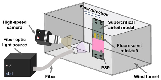
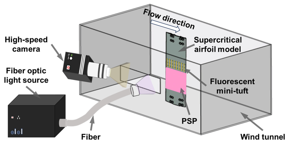
The image acquisition system mainly consists of an Andor Zyla 5.5 high-speed camera and a dual-excitation-band composite light source. The camera has an effective pixel count of 2560 × 2160 and a pixel size of 6.5 μm × 6.5 μm. It is equipped with a Nikon lens and a 500 nm high-pass filter, enabling simultaneous acquisition of the emission light from the fluorescent mini-tufts and the PSP coating. The self-developed composite light source is mainly composed of a light source host, an optical transmission module, and a light output module. The light source host uses a dichroic mirror to mix excitation light at two different wavelengths (400 nm and 460 nm), thereby satisfying simultaneous measurement of the fluorescent mini-tufts and PSP. The wind tunnel test model and the installation of the acquisition system are shown in Figure 2.
Figure 2.
Schematic diagram of experimental system.
2.2. Fluorescent Mini-Tuft Preparation and Taping Method
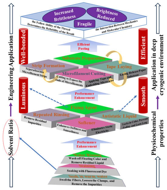
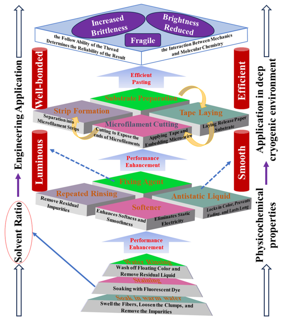
The Reynolds-number effect on shock buffet is significant, and precise assessment of the shock buffet onset is typically conducted in cryogenic, high-Reynolds-number facilities. In the extreme testing environment of such facilities (with freestream total temperatures as low as 110 K), conventional fluorescent mini-tufts become brittle and struggle to maintain excellent following capability and fluorescence brightness. In practice, any subtle process defect can be sharply magnified under extreme cryogenic conditions, thereby inducing chain effects such as mini-tuft brittle fracture, fluorescence quenching, or interfacial debonding. As shown in Figure 3, this paper develops a cryogenic fluorescent mini-tuft process-based preparation technique that combines high stability, adaptability, and repeatability, comprehensively optimizing and enhancing the preparation process and key control mechanisms of conventional fluorescent mini-tuft.
Figure 3.
Flowchart of preparing and taping fluorescent mini-tufts using a wide temperature range (The dotted arrows indicate the function/purpose of performing the corresponding step, while the other arrows indicate the sequence in which each step is performed).
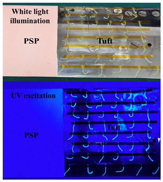
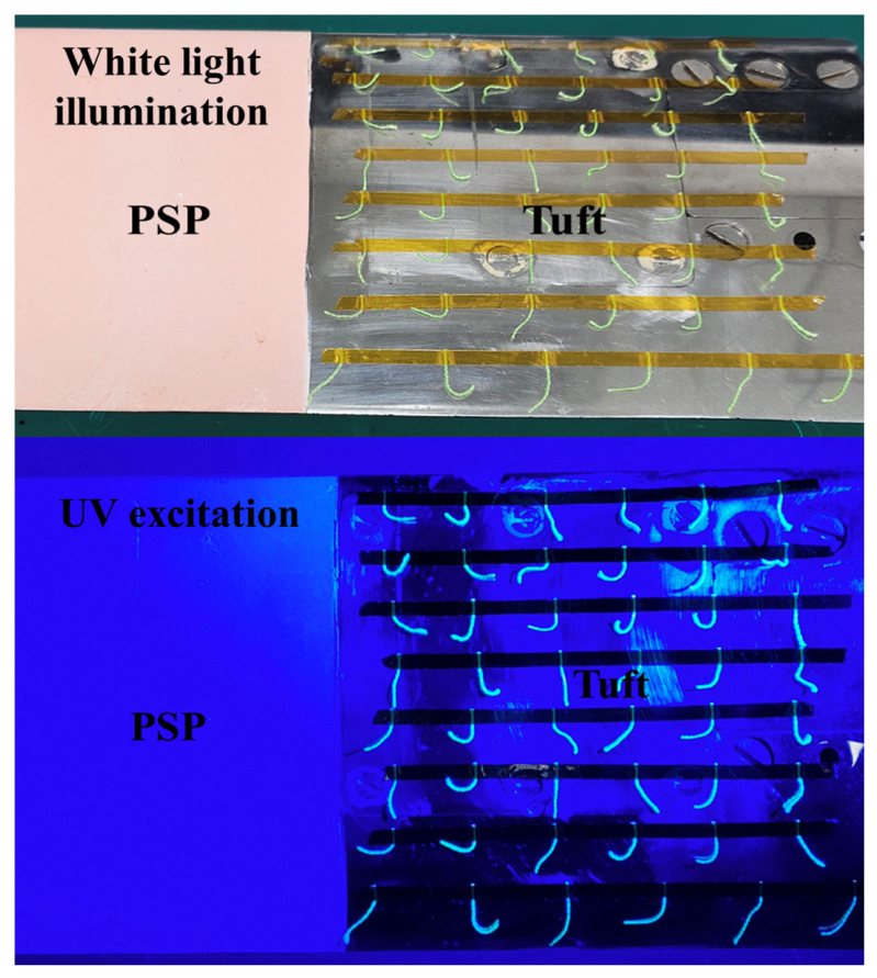
Figure 4 presents macro photographs of the mini-tufts in the visible range (under white light illumination) and under UV excitation, allowing a direct assessment of their morphological uniformity and fluorescence distribution. The luminophore used in this work is a fluorescein derivative, and the substrate is silk fiber with a diameter of 0.05 mm. The fabrication procedure consists of three core steps: (1) basic treatment—by controlling the dye concentration (mixed with purified water at a 1:2 ratio), temperature (40 °C), and time (90 min), uniform loading of fluorescent molecules onto the fiber is achieved; (2) performance enhancement—sequential treatments of dye fixing, softening, and antistatic finishing are applied to maintain the tufts’ flexibility and prevent brittle fracture at a cryogenic temperature of 110 K, while avoiding fluorescence decay; (3) engineering application—the tufts are fixed onto a release paper substrate using Kapton low-temperature ultra-thin tape, cut into strips, and then directly attached to the model surface. The entire process ensures reliable measurements with the mini-tufts under low-temperature, high-Reynolds-number conditions.
Figure 4.
Fluorescent mini-tuft luminescence image.
2.3. Digital Dynamic Flow Pattern Generation of Fluorescent Mini-Tufts
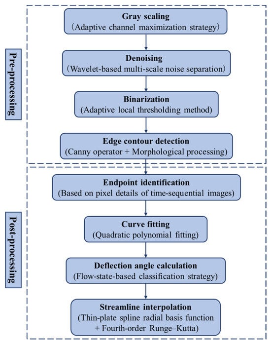
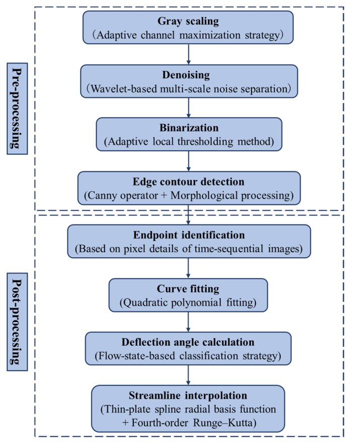
Typically, fluorescent mini-tufts serve only as auxiliary data for qualitative analysis of flow field structures. In this paper, based on advanced computer vision image recognition technology, we realize digital dynamic flow pattern and surface flow field reconstruction from fluorescent mini-tufts, transforming discrete, ambiguous, and qualitative visual information into a continuous, unified, and quantifiable dynamic flow pattern, thereby providing an important reference for the quantitative characterization of boundary-layer separation characteristics. The digital flow field reconstruction from fluorescent mini-tuft images consists of two parts: pre-processing and post-processing. The specific process and method are shown in Figure 5.
Figure 5.
Flowchart of digital flow pattern reconstruction from fluorescent mini-tufts.
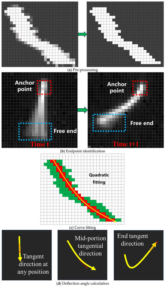
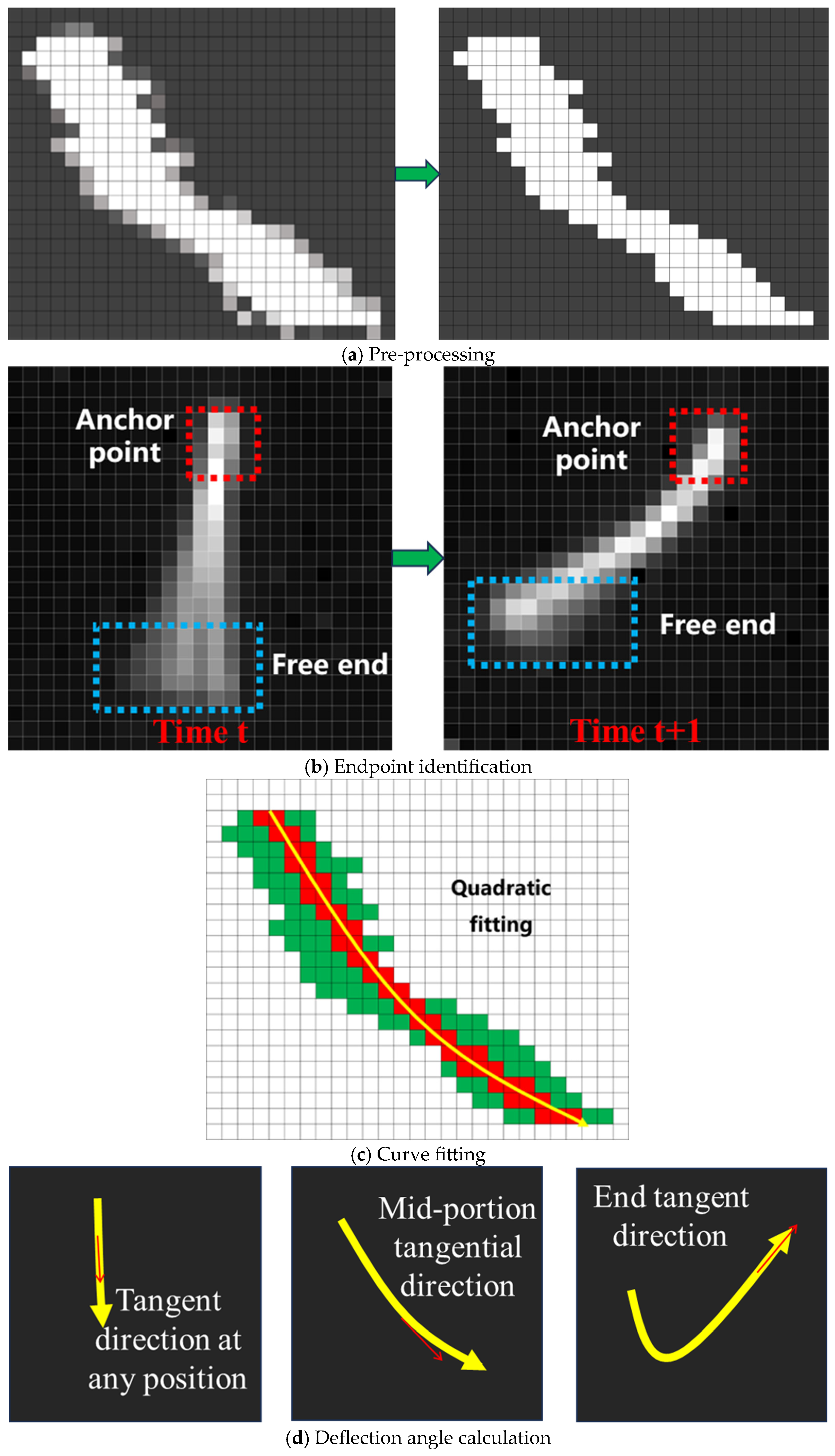
The results of each step in the aforementioned image processing are shown in Figure 6. The purpose of pre-processing is to highlight the contours of the fluorescent mini-tufts, enhance the contrast between the target and the background, accurately extract the morphological features of the fluorescent mini-tufts, eliminate random noise points caused by test environment interference (e.g., stray light) and electronic device noise (e.g., dark current), and reduce computational complexity. The adaptive thresholding method is used for grayscaling and binarization operations. The fluorescence signal intensity of each pixel is analyzed across the three channels (R, G, B) to ensure sharpness of the mini-tuft edges, providing high-quality input data for subsequent steps. Then, wavelet transform decomposition is applied to image information at different scales to separate the target from noise. Combined with the Canny operator for mini-tuft contour detection, the method finally outputs a continuous, closed, single-pixel-wide mini-tuft contour map that accurately reflects the positional information and morphological characteristics of the mini-tufts, as shown in Figure 6a. The purpose of post-processing is to achieve quantitative output of flow field information through steps such as endpoint identification (as shown in Figure 6b), fluorescent mini-tuft curve fitting (as shown in Figure 6c), and classification-based deflection angle calculation (as shown in Figure 6d). Based on the variation characteristics of pixel brightness of fluorescent mini-tuft endpoints in images at adjacent time instants, the anchor points and free ends are distinguished. Next, the fluorescent mini-tufts are fitted to quadratic curves, and a classification-based calculation strategy is employed to obtain the flow direction information indicated by the fluorescent mini-tufts, corresponding to the tangent direction at a specific position on the quadratic curve. Finally, the digital reconstruction of the surface flow field is achieved using the fourth-order Runge–Kutta streamline tracing method.
Figure 6.
Fluorescent mini-tuft processing results.
This paper adopts a method combining Thin-Plate Spline Radial Basis Function (TPS-RBF) and fourth-order Runge–Kutta (RK4) streamline tracing, which enables high-precision reconstruction of continuous vector fields and calculation of streamline trajectories from sparse and irregular discrete sampling data.
(1) Continuous direction field reconstruction using TPS-RBF; given N tuft sampling positions xi = (xi, yi)T ∈ R2 and the surface flow direction vectors di = (dxi, dyi)T inferred from tuft deflection angles, where each di is a unit vector representing the tangential direction of the surface streamline at that point. Because tuft visualization does not provide flow speed information and we focus on the geometric shape of streamlines (rather than time-parameterized trajectories), we define the reconstructed direction field as D(x) = (dx(x), dy(x))T and take V(x) = D(x) for streamline integration; the streamline shape depends only on the direction ratios, not on the magnitude.
The two components dx(x) and dy(x) are interpolated independently. Taking dx(x) as an example, the TPS-RBF interpolant takes the form
where ϕ(r) = r2 log r (defined as 0 at r = 0), p(x) = (1, x, y)T, and λi, c are coefficients. The interpolation conditions dx(xi) = dxi, together with orthogonality conditions ∑λi = ∑λixi = ∑λiyi = 0, lead to the linear system:
where Kij = ϕ(||xi − xj||), P contains rows (1, xi, yi), and dx = (d1x, …, dNx)T. Solving yields a globally smooth, twice-differentiable direction field component that minimizes bending energy. The same procedure is applied to dy(x).
The resulting interpolated direction field D(x) may not preserve unit length everywhere. However, because streamline integration depends only on the direction ratio dy/dx, using the non-normalized D(x) as V(x) in RK4 integration yields correct streamline shapes. If a strictly unit direction field is desired, one can normalize at each step; both approaches are equivalent.
(2) RK4 streamline tracing. With the continuous direction field V(x) = (dx(x), dy(x))T, streamlines satisfy the ODE initial-value problem:
We integrate using the fourth-order Runge–Kutta (RK4) method:
The local truncation error is O(h5) and global error O(h4), providing high accuracy for tracing curved surface flow structures.
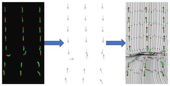
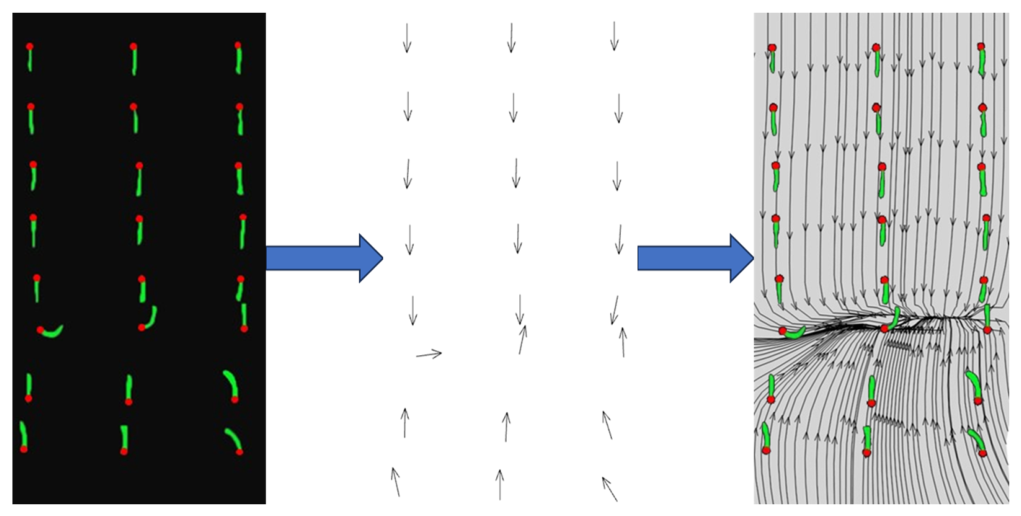
This combined strategy not only overcomes the difficulties of insufficient resolution and uneven distribution of measured data, but also provides a high-fidelity visualization foundation for subsequent flow feature analysis (such as vortex identification, transport path prediction). As shown in Figure 7, the fluorescence mini-tuft interpolation results obtained using this method are presented.
Figure 7.
Reconstruction process of fluorescent mini-tuft flow field (The arrows indicate the direction of the fluorescent mini-tufts. The green pattern represents the fluorescent mini-tufts themselves. The red dots indicate the fixed ends of the fluorescent mini-tufts).
3. Results and Discussion
The existing literature indicates that when the adverse pressure gradient induced by the shock exceeds the bearing capacity of the boundary layer, it leads to its separation. Low-energy, unstable flow separation is the core driving force for the generation, development, and maintenance of shock oscillation. The two phenomena interact and couple with each other, forming a self-sustaining, closed-loop dynamic process in which “separation disturbs the shock, which in turn intensifies separation fluctuations via shock oscillation”. From the perspective of detailed flow field evolution, the shock location determines the spatial distribution of the separation onset point [24]. Therefore, in this paper, the deflection characteristics of fluorescent mini-tufts in a shock-induced separated flow field are used to indirectly characterize the shock buffet onset.
To verify the reliability of assessing the shock buffet onset based on the dynamic flow pattern of fluorescent mini-tufts, simultaneous PSP and fluorescent mini-tuft measurement tests were conducted in the 0.3 m high-Reynolds-number transonic wind tunnel. The test Mach number ranged from 0.6 to 0.9, the freestream total temperature from 110 K to 280 K, and the Reynolds number from 5.5 × 10⁶ to 8.5 × 10⁶. The buffet onset Mach number was measured using PSP and fluorescent mini-tuft techniques at an angle of attack of 3°.
3.1. Fluorescent Mini-Tuft Flow Pattern Analysis at Different Mach Numbers
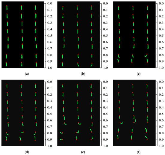
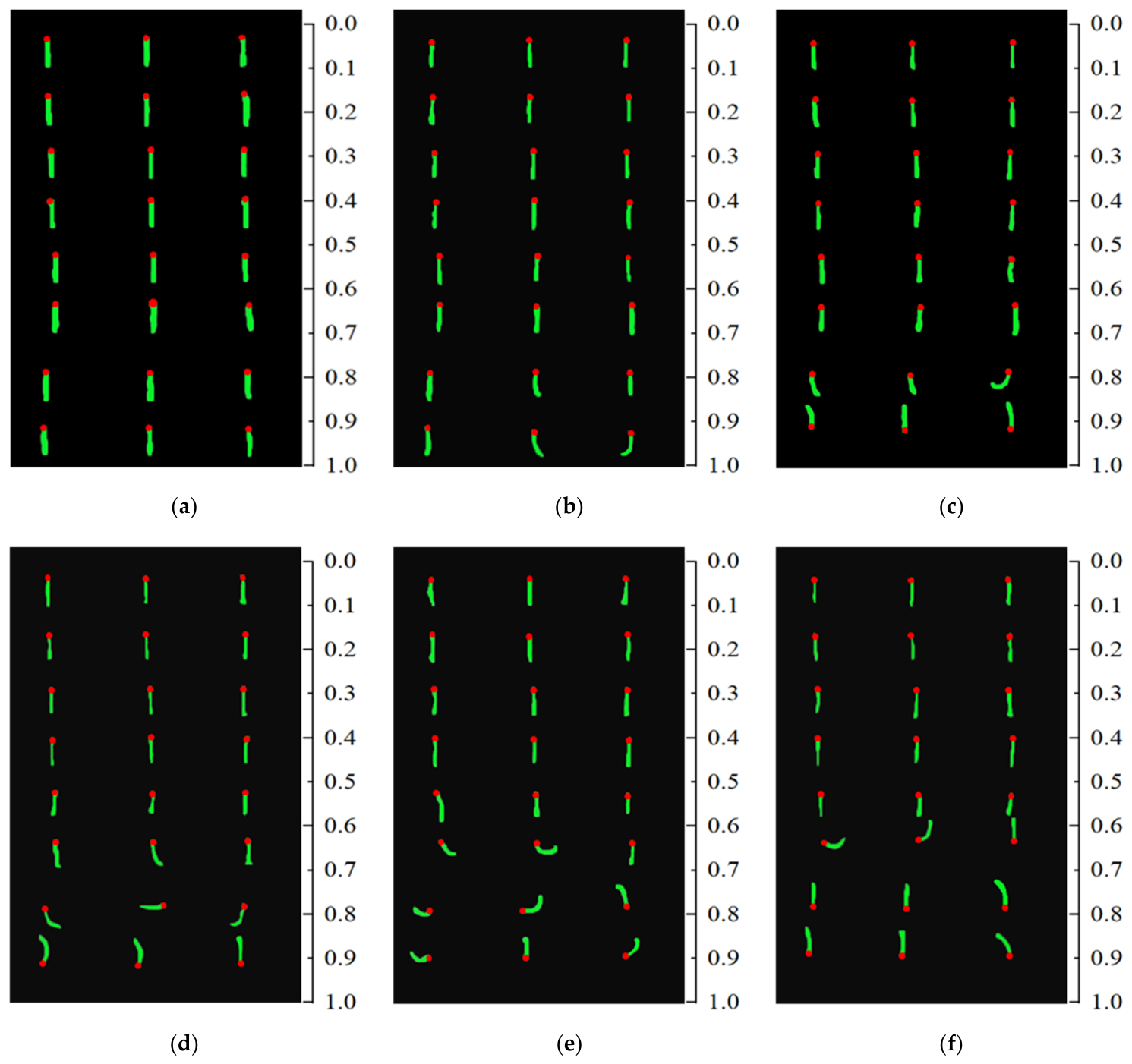
Figure 8 shows fluorescent mini-tuft images at typical time instants under freestream total temperature T0 = 110 K and Mach numbers Ma = 0.6, 0.7, 0.76, 0.8, 0.86, and 0.9. It can be seen from the figure that at Ma = 0.6 and 0.7, the fluorescent mini-tufts all point in the freestream direction without noticeable bending. Only at Ma = 0.7 does a very slight deflection occur at the trailing edge of the wing. When the Mach number increases to 0.76, the fluorescent mini-tufts in the region x/c = 0.2~0.82 all point in the freestream direction, indicating attached flow. Deflection begins after the 80% chord position, and the mini-tufts at the trailing edge point are completely opposite to the freestream direction, indicating flow separation at the wing trailing edge caused by an adverse pressure gradient. As the Mach number increases, the chordwise position where the fluorescent mini-tufts start to deflect moves further forward. At Ma = 0.86, the flow separation region expands further, and the fluorescent mini-tufts show obvious deflection at x/c ≈ 0.7. Experimental observations reveal that at this condition, the mini-tufts oscillate with extremely large amplitude and very high frequency in the reverse flow direction, representing a typical fluorescent mini-tuft state under fully separated flow. At Ma = 0.9, the fluorescent mini-tufts already exhibit a reverse flow pattern at x/c ≈ 0.7, and the separation region and its intensity on the upper surface of the wing further increase.
Figure 8.
Fluorescent mini-tuft images under typical conditions at T0 = 110 K: (a) Ma = 0.6, (b) Ma = 0.7, (c) Ma = 0.76, (d) Ma = 0.8, (e) Ma = 0.86, (f) Ma = 0.9.
Therefore, it can be concluded that when the wind tunnel freestream total temperature is reduced from 280 K to 110 K, the fluorescent mini-tufts exhibit good followability and no detachment under the deep cryogenic and strong scouring environment. The proposed preparation and taping process for fluorescent mini-tufts has good applicability and can dynamically and clearly reveal the surface flow structures on a supercritical airfoil in the subsonic to transonic range. Next, we will discuss the shock position indicated by PSP and the flow state results revealed by the fluorescent mini-tufts. Here, the shock position from PSP is determined as the peak position of the pressure gradient calculated pixel-wise; the separation location is taken as the position where the chordwise component of the interpolated tuft direction data becomes zero, and the process of this component decreasing from positive to zero is considered as the region where different flow states coexist [25].
3.2. Comparison of Fluorescent Mini-Tufts and PSP Results
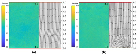
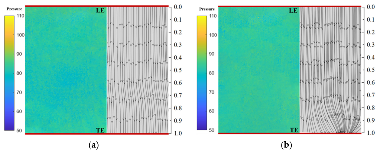
Figure 9 presents the PSP pressure distribution and the digital surface streamlines reconstructed from fluorescent mini-tuft images at Mach numbers of 0.6 and 0.7. From the PSP pressure distribution contours in the figure, it can be seen that under Ma = 0.6 and 0.7 conditions, after the flow stagnates at the leading edge stagnation point, it accelerates along the upper surface. The pressure is at a moderate level, with the most obvious flow acceleration occurring in the region between the leading edge and the chordwise position x/c = 0.8, where the pressure is relatively low. After x/c = 0.8, the pressure begins to recover gradually, without the sharp pressure rise typically seen following a shock. From the digital streamline results obtained from the fluorescent mini-tufts on the right, it can be seen that at Ma = 0.6, the streamlines over the entire wing surface are straight, with no fluctuation in the flow field. At Ma = 0.7, only slight spanwise deflection and convergence of streamlines appear near the trailing edge, without severe bending or large-scale separation induced by a shock. This indicates good flow attachment and a stable accelerating state, which is in good agreement with the PSP results.
Figure 9.
Wind tunnel test results at T0 = 110 K, AOA = 3°: (a) Ma = 0.6, (b) Ma = 0.7.
Figure 10 presents the PSP pressure distribution and the digital streamlines from fluorescent mini-tufts at Mach numbers of 0.76 and 0.8. When the Mach number increases to 0.76, the flow accelerates from the low-pressure region near the leading edge up to x/c ≈ 0.66, after which the pressure begins to recover. Compared with the Ma = 0.7 case, the pressure variation is more pronounced, but a strong adverse pressure gradient has not fully formed; only a weak shock is generated, and no significant shock oscillation occurs. From the streamline plot, it can be seen that before x/c = 0.67, the streamlines are uniformly distributed. After x/c = 0.67, the streamlines begin to show noticeable deflection in the spanwise direction and converge downward, eventually forming a clear vortex structure and reverse flow near x/c ≈ 0.85. This is because the pressure begins to rise significantly near x/c ≈ 0.7, generating a weak shock in that region, which in turn leads to local flow separation. The PSP and streamline results are in good agreement. As shown in Figure 10b, when the Mach number increases to 0.8, the pressure begins to recover at x/c ≈ 0.62, forming a clear adverse pressure gradient and generating a shock. Comparison with the streamline results shows that the shock induces local boundary-layer separation. Compared with the Ma = 0.76 case, the separation region is larger and located further upstream.
Figure 10.
Wind tunnel test results under conditions of T0 = 110 K, AOA = 3°: (a) Ma = 0.76, (b) Ma = 0.8.
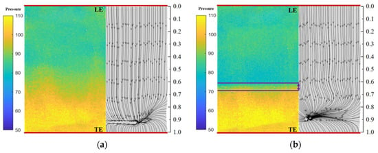
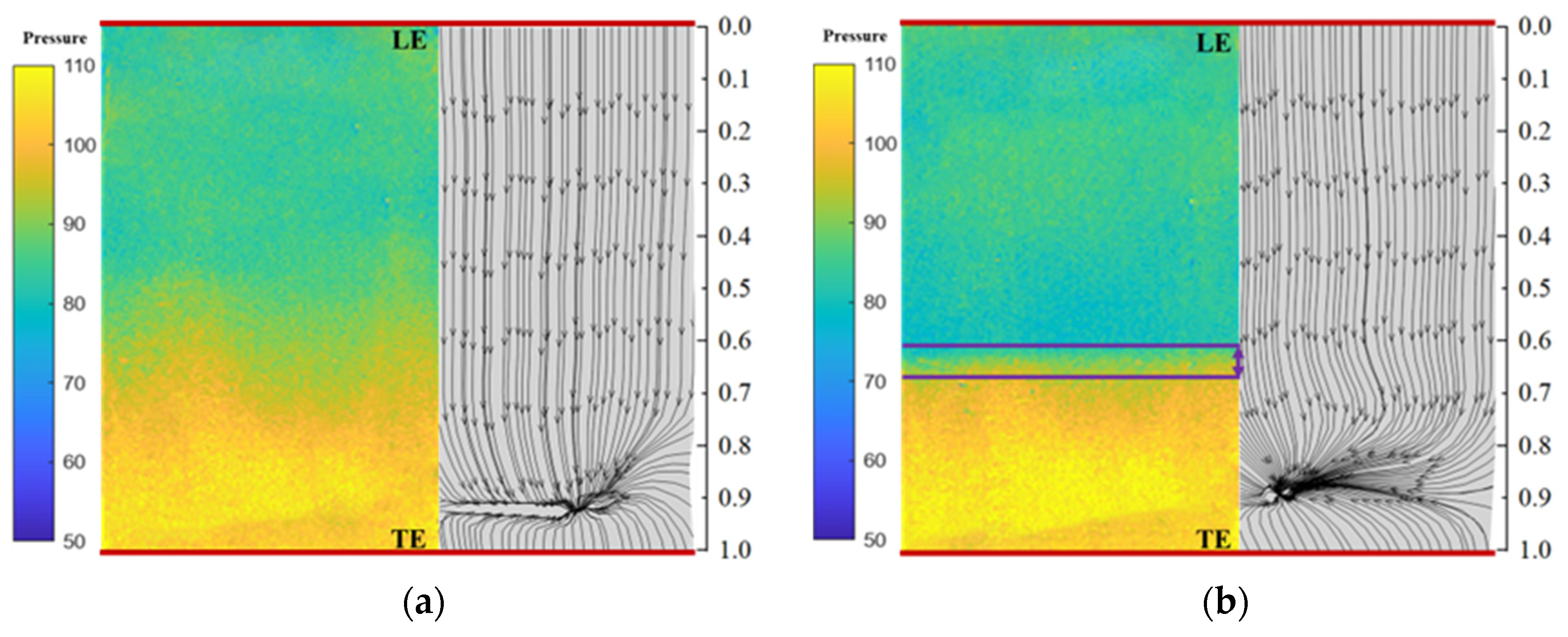
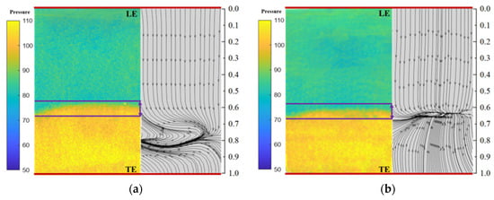
Figure 11 presents the PSP pressure distribution and the digital streamlines from fluorescent mini-tufts at Mach numbers of 0.86 and 0.9. As shown in Figure 11a, when the Mach number increases to 0.86, the flow enters the low-pressure acceleration region from the leading edge and begins transitioning to the high-pressure region at x/c ≈ 0.58. Under this condition, the adverse pressure gradient is larger and located further upstream; the flow begins to decelerate until pressure recovery. From the streamline plot, it can be seen that as the Mach number increases, the separation region shifts further upstream and becomes larger, which is caused by the upstream movement and intensification of the shock. As shown in Figure 11b, at Ma = 0.9, the separation region moves significantly upstream, and the mean position of the adverse pressure gradient is generally consistent with the trend observed at Ma = 0.86 and 0.8.
Figure 11.
Wind tunnel test results under conditions of T0 = 110 K, AOA = 3°: (a) Ma = 0.86, (b) Ma = 0.9 (The purple line represents the range of changes in the position of the shock).
Figure 12 shows the instantaneous shock positions obtained by PSP under different Mach number conditions. It can be seen from the figure that at Ma = 0.76, a weak shock is generated near x/c = 0.66, and the degree of shock oscillation is not significant. When Ma exceeds 0.8, the shock intensity increases and exhibits periodic oscillation on the airfoil surface. It should be noted that the image acquisition frame rate was 143 Hz. Spanwise averaging was performed using data acquired at six uniformly distributed spanwise measurement locations, and the presented results are the average over these six positions.
Figure 12.
Shock position variation at different Mach numbers.
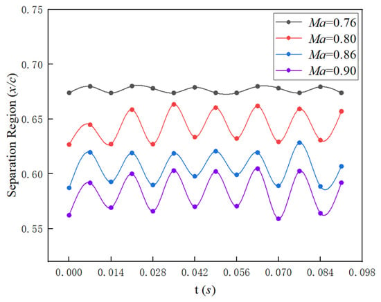
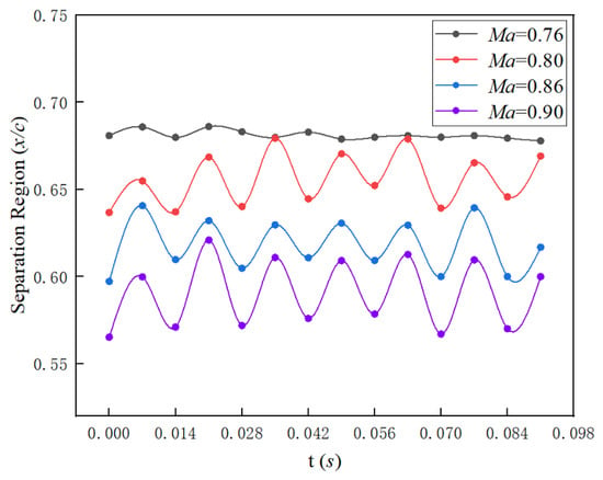
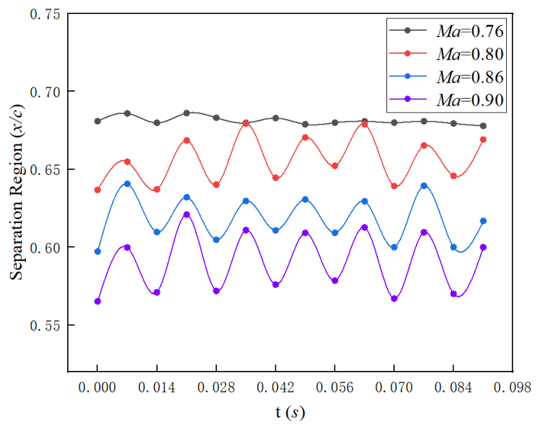
As shown in Figure 13, the separation onset locations were extracted from mini-tuft images under different Mach number conditions. It can be observed that when Ma = 0.76, the instantaneous position of the separation region remains essentially near x/c = 0.67. As the Mach number increases to 0.8, due to the onset of shock buffet, the separation region induced by the shock oscillates periodically in synchrony with the shock position. Furthermore, as the Mach number increases further, the position of the separation region shifts progressively upstream.
Figure 13.
Time-resolved evolution of separation boundaries visualized by fluorescent mini-tufts under different Mach number conditions.
Comparing the separation region positions with the shock locations determined from the peak pressure gradient of PSP in Figure 12, the results show that at Ma = 0.76, the average relative deviation in chordwise position between the two is approximately 0.68%, indicating a good correspondence between the shock position and the downstream separation region. At Ma = 0.8 and 0.86, the deviations gradually increase, respectively. This is mainly attributable to two factors: first, the strong unsteady characteristics of shock buffet; second, the lower spatial resolution of fluorescent mini-tuft flow visualization compared to PSP, which introduces a systematic bias between the two measurement techniques. Nevertheless, the trend of flow field variation remains consistent. At Ma = 0.9, the deviation decreases to approximately 1.29%, which is directly related to the fact that the unsteady intensity of shock buffet under this condition is lower than that at Ma = 0.8 and 0.86.
In summary, under the conditions of freestream total temperature 110 K and angle of attack 3°, the buffet onset Mach number for this model lies between 0.76 and 0.8, and the PSP results are in good agreement with the fluorescent mini-tuft results. It is worth noting that, compared with techniques such as PSP and oil flow visualization, the spatial resolution of fluorescent mini-tuft measurements is lower, and there is some error in streamline interpolation, which may to some extent enlarge or reduce the separation and reattachment boundaries. Nevertheless, the advantages of this method—such as local high efficiency, convenience, low cost, and strong adaptability to extreme conditions—can provide an important reference for the study of buffet characteristics of advanced aircraft.
4. Conclusions
To solve the problems of traditional experimental measurement methods, such as discrete measurement points, insufficient capability for identifying flow characteristics, and high costs, this paper develops a shock buffet onset assessment technique based on fluorescent mini-tuft dynamic flow patterns. The reliability of this method is verified through wind tunnel tests. The main conclusions are as follows:
- (1)
- The fluorescent mini-tuft preparation and taping process developed in this paper exhibits good adaptability under the extreme conditions of wide temperature range and strong scouring. Within the Mach number range of 0.6~0.9 and total temperature range of 110~280 K, the fluorescent mini-tufts with a diameter of approximately 0.05 mm demonstrate good flow-following capability and no detachment.
- (2)
- The digital flow patterns of the fluorescent mini-tufts obtained using computer vision algorithms clearly reveal the location and area of boundary-layer separation, and are in good agreement with cryogenic PSP results.
- (3)
- The overall trend of the influence of Mach number on flow separation is “earlier onset position, larger region, and higher strength” with increasing Mach number. As the Mach number increases, the chordwise position where the fluorescent mini-tufts begin to deflect moves forward, and both the size of the separation region and the amplitude of mini-tuft oscillation gradually increase, reflecting the intensification of separation strength and flow disturbance with increasing Mach number.
In the future, the algorithm for automatically identifying fluorescent mini-tuft separation and attachment will be further developed, integrating CFD results to improve the interpolation accuracy of digital streamlines through advanced flow field reconstruction techniques, and extracting more useful information from the fluorescent mini-tuft results, so as to provide richer data for the study of shock buffet mechanisms of advanced large aircrafts.
Author Contributions
Conceptualization, G.L. and J.W.; methodology, B.Q., J.W. and G.L.; validation, S.G., L.Y., P.Q. and B.Q.; formal analysis, B.Q.; investigation, B.Q.; data curation, B.Q., L.Y. and S.G.; writing—original draft preparation, B.Q.; writing—review and editing, J.W., D.L., H.D. and G.L.; visualization, B.Q., S.G. and L.Y.; funding acquisition, G.L. and J.W. All authors have read and agreed to the published version of the manuscript.
Funding
This research was supported by the National Natural Science Foundation of China (52476037, U24A20141), the Foundation of State Key Laboratory of Aerodynamics (SKLA-2024-KFKT-4-005).
Data Availability Statement
The data that support the findings of this study are available from the corresponding author upon reasonable request.
Conflicts of Interest
The authors declare no conflicts of interest.
Abbreviations
The following abbreviations are used in this manuscript:
| PSP | Pressure Sensitive Paint |
| RANS | Reynolds-Averaged Navier–Stokes |
| LES | Large Eddy Simulation |
| URANS | Unsteady Reynolds-Averaged Navier–Stokes |
| DMD | Dynamic Mode Decomposition |
| IDDES | Improved Delayed Detached Eddy Simulation |
| PIV | Particle Image Velocimetry |
| LDV | Laser Doppler Velocimetry |
| c | Airfoil chord length |
| b | Airfoil span length |
| DDES | Delayed Detached Eddy Simulation |
| Ma | Mach number |
| Re | Reynolds number |
| AOA | Attack angle |
| T0 | Total temperature |
References
- Dou, Z.H.; Wu, J.Q.; Gao, C.Q.; Zhang, W.W. Transonic buffet characteristics and Reynolds number effects of CHN-T2 standard model. Acta Aerodyn. Sin. 2024, 42, 93–107. [Google Scholar] [CrossRef]
- Giannelis, F.N.; Vio, A.G.; Levinski, O. A review of recent developments in the understanding of transonic shock buffet. Prog. Aerosp. Sci. 2017, 92, 39–84. [Google Scholar] [CrossRef] [Scilit]
- Lee, K.H.B.; Murty, H.; Jiang, H. Role of Kutta waves on oscillatory shock motion on an airfoil. AIAA J. 2012, 32, 789–796. [Google Scholar] [CrossRef] [Scilit]
- Lee, B. Self-sustained shock oscillations on airfoils at transonic speeds. Prog. Aerosp. Sci. 2001, 37, 147–196. [Google Scholar] [CrossRef] [Scilit]
- Chuanqiang, G.; Weiwei, Z. Transonic aeroelasticity: A new perspective from the fluid mode. Prog. Aerosp. Sci. 2020, 113, 100596. [Google Scholar] [CrossRef] [Scilit]
- Xiao, F.; Meng, X.; Chen, T.; Wu, D.; Liu, X.; Dai, Y. Development and key technologies of mechanism and control for transonic buffet. Acta Aerodyn. Sin. 2026, 44, 1–14. [Google Scholar] [CrossRef]
- Pasquale, D.D.; Prince, S. Passive Transonic Shock Control on Bump Flow for Wing Buffet Suppression. Aerospace 2023, 10, 569. [Google Scholar] [CrossRef] [Scilit]
- Zhang, W.W.; Gao, C.Q.; Ye, Z.Y. Research advances of wing/airfoil transonic buffet. Acta Aeronaut. Astronaut. Sin. 2015, 36, 1056–1075. [Google Scholar]
- Zhang, S.; Deng, F.; Ni, Z. Numerical Analysis of Shock Control Bumps for Delaying Transonic Buffet Boundary on a Swept Wing. Aerospace 2026, 13, 98. [Google Scholar] [CrossRef] [Scilit]
- Willhite, P.; Jsper, D.; Romer, W. A Critical Evaluation of CFD Predictions of Full Aircraft Drag Increments. In Proceedings of the 26th AIAA Fluid Dynamics Conference, San Diego, CA, USA, 19–22 June 1995. AIAA Paper 95-2289. [Google Scholar] [CrossRef] [Scilit]
- Walters, D.K.; Bhushan, S.; Alam, M.F.; Thompson, D.S. Investigation of a Dynamic Hybrid RANS/LES Modelling Methodology for Finite-Volume CFD Simulations. Flow Turbul. Combust. 2013, 91, 643–667. [Google Scholar] [CrossRef] [Scilit]
- Gao, C.Q.; Zhang, W.W. Numerical simulation and modal analysis of transonic buffet flow over wings. Acta Aeronaut. Astronaut. Sin. 2019, 40, 122597. [Google Scholar] [CrossRef]
- Chwalowski, P.; Massey, S.J.; Jacobson, K.; Silva, W.A.; Stanford, B. Progress on transonic flutter and shock buffet computations in support of the Third Aeroelastic Prediction Workshop. In Proceedings of the AIAA SciTech 2021 Forum; AIAA: Reston, VA, USA, 2021. [Google Scholar] [CrossRef] [Scilit]
- Kramer, B.; Grover, P.; Boufounos, P.; Nabi, S.; Benosman, M. Sparse Sensing and DMD-Based Identification of Flow Regimes and Bifurcations in Complex Flows. SIAM J. Appl. Dyn. Syst. 2017, 16, 1164–1196. [Google Scholar] [CrossRef] [Scilit]
- Brunton, S.L.; Proctor, J.L.; Kutz, J.N. Compressive sampling and dynamic mode decomposition. J. Comput. Dyn. 2015, 2, 165–191. [Google Scholar] [CrossRef] [Scilit]
- Masini, L.; Timme, S.; Peace, A.J. Analysis of a civil aircraft wing transonic shock buffet experiment. J. Fluid Mech. 2019, 884, A1. [Google Scholar] [CrossRef] [Scilit]
- Victor, P.M.; Gabriel, C.M.; Cristina, F.M.; Mircea, B. Signal processing and analysis in a buffet onset wind tunnel campaign. INCAS Bull. 2015, 7, 129–136. [Google Scholar] [CrossRef] [Scilit]
- Sugioka, Y.; Koike, S.; Nakakita, K.; Numata, D.; Nonomura, T.; Asai, K. Correction to: Experimental analysis of transonic buffet on a 3D swept wing using fast-response pressure-sensitive paint. Exp. Fluids 2020, 61, 144. [Google Scholar] [CrossRef] [Scilit]
- He, B.; Li, G.; Zhou, F.; Liu, D.; Xiang, X. Application of colour fluorescent oil flow visualization for a high speed cavity. J. Phys. Conf. Ser. 2021, 1786, 012049. [Google Scholar] [CrossRef] [Scilit]
- Saile, D.; Kühl, V.; Gülhan, A. Aerodynamic excitations in the near wake of space launchers: Insights from hot-flow experiments using high-speed PIV. Exp. Fluids 2026, 67, 33. [Google Scholar] [CrossRef] [Scilit]
- Darisse, A.; Lemay, J.; Benaïssa, A. LDV measurements of well converged third order moments in the far field of a free turbulent round jet. Exp. Therm. Fluid Sci. 2013, 44, 825–833. [Google Scholar] [CrossRef] [Scilit]
- Sun, B.; Shehzad, M.; Willert, C.; Foucaut, J.-M.; Cuvier, C.; Ostovan, Y.; Atkinson, C.; Soria, J. High spatial resolution 2C-2D PIV measurements using a 47 MPx sensor of high Reynolds number turbulent boundary layer flow. In Proceedings of the 20th International Symposium on Application of Laser and Imaging Techniques to Fluid Mechanics; International Symposium on Application of Laser and Imaging Techniques to Fluid Mechanics: Lisbon, Portugal, 2022. [Google Scholar]
- Qiao, P.; Wu, J.; Huang, H.; Li, G.; Li, D.; Du, H. Experimental Investigation on Temperature Effects of Cryogenic Pressure-Sensitive Paint. Aerospace 2025, 12, 329. [Google Scholar] [CrossRef] [Scilit]
- Gao, S.; Dong, H.; Wu, J.; Liu, D.; Li, G.; Yang, L.; Kong, W.; Gong, M.; Zhao, Y.; Gu, Y. Study on Reynolds Number Effects on Transonic Buffet of Supercritical Airfoils with Transition Considerations. Aerospace 2025, 13, 1. [Google Scholar] [CrossRef] [Scilit]
- Vey, S.; Lang, H.M.; Nayeri, C.N.; Paschereit, C.O.; Pechlivanoglou, G. Extracting quantitative data from tuft flow visualizations on utility scale wind turbines. J. Phys. Conf. Ser. 2014, 524, 012011. [Google Scholar] [CrossRef] [Scilit]
Disclaimer/Publisher’s Note: The statements, opinions and data contained in all publications are solely those of the individual author(s) and contributor(s) and not of MDPI and/or the editor(s). MDPI and/or the editor(s) disclaim responsibility for any injury to people or property resulting from any ideas, methods, instructions or products referred to in the content. |
© 2026 by the authors. Licensee MDPI, Basel, Switzerland. This article is an open access article distributed under the terms and conditions of the Creative Commons Attribution (CC BY) license.