Data-Driven LPV Modeling via Parametric DMD and Predictive Control of Highly Flexible Aircraft

Abstract

This paper presents a method of data-driven parametric dynamic mode decomposition (p-DMD) to derive a linear parameter-varying reduced-order model (LPV-ROM) and predictive control for the nonlinear aeroelasticity of highly flexible aircraft. It directly uses the data snapshots obtained at varying flight conditions and encodes a nonlinear model’s polynomial dependency on flight conditions to produce a polynomial-dependent LPV-ROM. The modeling method can handle not only equilibrium flight conditions but also continuously varying flight conditions. In numerical studies, the proposed data-driven p-DMD modeling is applied to a highly flexible cantilever wing perturbed around equilibrium conditions and a flexible aircraft with time-varying angles of attack in dynamic maneuvers. The numerical results demonstrate that the current p-DMD model can capture the non-equilibrium (or transient) aeroelastic and flight dynamic behaviors of highly flexible aircraft in both time and frequency domains with over 95% accuracy in the simulated representative cases. Accuracy is quantified by the normalized root mean square error (NRMSE) in the time domain and the normalized error between the frequency responses over the frequency range of interest. The data-driven reduced-order model is further implemented in predictive control to suppress the vibrations excited by Dryden gust disturbances. The simulation results demonstrate that for a Dryden gust profile, data-driven predictive control can suppress the strains by 18.34% as quantified by the reduction in the root mean square of strains compared to the uncontrolled case.

1. Introduction

High-aspect-ratio slender wings are widely considered as a next-generation design aimed at high-altitude, long-endurance (HALE) flights due to their excellent performance and efficiency. Accurate and efficient modeling tools are essential for the design, optimization, and control of these highly flexible wings. The nonlinear aeroelasticity of highly flexible wings, coupled with rigid-body dynamics, must be comprehensively addressed in dynamic modeling, stability analysis, and closed-loop controls. However, the complex fluid–structure–control interactions (FSCIs) induced by the flexible structure pose significant challenges to aeroelastic modeling and active control.

First of all, dynamic modeling of nonlinear aeroelasticity across a range of flight conditions is challenging, even for simple wing geometries. Linearization is the most commonly used method to analyze aircraft stability, predict dynamic responses, and develop control-oriented models [1]. However, linearization typically assumes small perturbations around an equilibrium (trim) flight condition, making it unsuitable for the large and nonlinear wing deformations of flexible structures or unsteady flight conditions in dynamic maneuvers. Linear parameter-varying (LPV) modeling offers an effective approach to model nonlinearity by interpolating models linearized at a series of gridded flight conditions [2,3]. Subsequently, an LPV controller can be designed to be parameter-dependent, allowing for smooth scheduling of controller gains at varying flight conditions [4].

Another challenge is developing parametric reduced-order models (ROMs) for different flight conditions that enable fast computations for predictions and control. At a trim flight condition, a high-fidelity model of FSCI can be reduced to a lower-order model through spectral analysis, preserving only the most significant modes. This process involves solving an eigenvalue problem and selecting a set of orthogonal modes for the reduced-order model. Existing works on parametric reduced-order modeling [5,6] typically repeat model reductions at gridded flight conditions and use interpolations to capture parametric dependency across various flight conditions. However, several issues need to be addressed in parametric model order reduction: (1) System stability can vary from being stable to unstable across different flight conditions; for example, a flexible vehicle can become unstable when flight speeds exceed a certain threshold [3]. These unstable modes must be included in the parametric ROM. (2) A complex conjugate pair can transition to two real-valued poles, or two real-valued poles can merge and split into a complex conjugate pair [7]. Therefore, eigenvalues and eigenvectors must be tracked and aligned at gridded flight conditions to ensure consistency of states among the fixed models. Several works have been developed to enforce the alignment of states in parametric ROMs [5,6]. These methods are often computationally heavy in the high-dimensional system rendered by the high-fidelity model.

In recent years, there has been growing interest in data-driven modeling of the nonlinear aeroelasticity of flexible wings. Various data-driven methods, such as those using neural networks [8] and Kriging [9], leverage large datasets obtained from experiments or numerical simulations to train input–output mappings without requiring physical knowledge. These approaches are particularly effective for complex, nonlinear systems where analytical models are difficult to establish. However, for safety-critical flight control applications, challenges remain when such models are used in a purely data-driven manner. In particular, they may lack explicit physical structure, making it difficult to provide guarantees on stability, robustness, and extrapolation beyond the training domain.

Data-driven methods that can render state-space models are of particular interest from a control perspective. Techniques such as identification methods or mode decomposition can be used to find the optimal reduced-order model that best approximates the system. The Eigensystem Realization Algorithm (ERA) [10] and Autoregressive with Exogenous Input (ARX) [11,12] have been developed to identify the model parameters of reduced-order models from datasets. However, neither ARX nor ERA encodes information about the physical states. When physical states are available, a physically interpretable state-space model can be obtained through various methods. Proper Orthogonal Decomposition (POD) aims to find a low-dimensional subspace of spatially orthogonal modes that best match dynamic responses [13,14]. Sparse Identification of Nonlinear Dynamics (SINDy) can produce a physically interpretable nonlinear model based on a library of nonlinear basis functions [15,16].

In particular, dynamic mode decomposition (DMD) is an equation-free method that can reveal the evolution of spatial modes and temporal dynamics from data snapshots. The DMD algorithm uses the data of dynamic responses obtained by perturbing equilibrium points to perform spectrum analysis and yields a Linear Time-Invariant (LTI) model [7,17]. Dynamic mode decomposition with control (DMDc) has been proposed and applied to flexible wings at different operating conditions [7]. To obtain ROMs, projection-based model reduction methods are often employed to retain the most significant modes [18].

Data-driven modeling for parameter-dependent ROMs over a range of flight conditions presents significant challenges, with the embedding of parameter dependency into the projection basis matrices being a critical issue to address. One method is to generate a ’global’ projection basis over the range of flight parameters. An alternative method is to generate ’local’ ROMs using a series of projection basis matrices and interpolate the local ROMs to form parametric ROMs. Adaptive sampling [19] and other interpolation methods, such as gappy-POD interpolation [20] and the Discrete Empirical Interpolation Method (DEIM) [21], have been developed for nonlinear parametric dependence. Balanced mode decomposition (BMD) has been developed using an oblique projection, where the projection basis space is shared to achieve state consistency, and the testing projection is chosen as parameter-dependent to obtain parametric models [17]. However, these methods still rely on the assumption of small wing deformations and perturbed equilibrium flight conditions. Therefore, the transient dynamics caused by varying flight conditions and large structure deformation are not fully captured, which calls for a new modeling method.

2. Nonlinear Aeroelasticity and Linear Modeling

This section provides a concise overview of nonlinear aeroelastic formulation and the conventional approach of linearizing and interpolating around equilibrium points to derive linear models and LPV models. The shortcomings and limitations of this traditional method will be discussed, leading to the motivation for the proposed approach.

Numerous efforts have been made to examine the nonlinear aeroelasticity of highly flexible aircraft. While refined models based on shell formulations may capture more details of deformations in morphing and geometrically complicated wings, a geometrically nonlinear beam theory is usually sufficient to establish an aeroelastic formulation for highly flexible aircraft. Palacios et al. [22] comprehensively discussed three types of beam formulations for the structural, aeroelastic, and flight dynamic analysis of highly flexible aircraft. By coupling a strain-based geometrically nonlinear beam formulation with the finite-state inflow theory [23,24,25], Cesnik and his colleagues established the nonlinear aeroelastic and flight dynamic formulation, now known as UM/NAST [26,27,28].

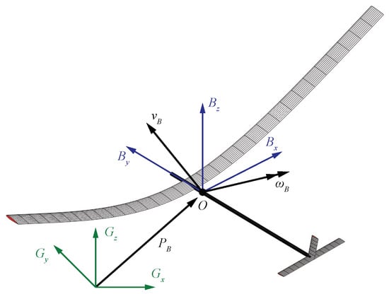
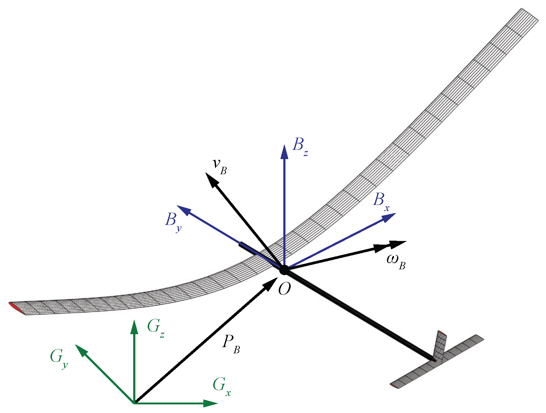
By following the strain-based approach [27,28], the coupled nonlinear aeroelasticity and flight dynamics of highly flexible aircraft (see Figure 1) are formulated as

$$\begin{array}{c}{\mathbf{M}}_{FF}\left(\mathit{\epsilon }\right)\ddot{\mathit{\epsilon }}+{\mathbf{M}}_{FB}\left(\mathit{\epsilon }\right)\dot{\mathit{\beta }}+{\mathbf{K}}_{FF}\mathit{\epsilon }={\mathbf{R}}_F\\ {\mathbf{M}}_{BF}\left(\mathit{\epsilon }\right)\ddot{\mathit{\epsilon }}+{\mathbf{M}}_{BB}\left(\mathit{\epsilon }\right)\dot{\mathit{\beta }}={\mathbf{R}}_B\\ \dot{\mathit{\zeta }}=-{\displaystyle \frac{1}{2}}{\mathbf{\Omega }}_{\mathit{\zeta }}\left(\mathit{\beta }\right)\mathit{\zeta }\\ {\dot{\mathbf{p}}}_B^G=\left[\begin{array}{cc}{\mathbf{C}}^{GB}\left(\mathit{\zeta }\right)& \mathbf{0}\end{array}\right]\mathit{\beta }\\ \dot{\mathit{\lambda }}={\mathbf{F}}_1(\dot{\mathit{\epsilon }},\mathit{\beta })\mathit{\lambda }+{\mathbf{F}}_2(\dot{\mathit{\epsilon }},\mathit{\beta })\left\{\begin{array}{c}\dot{\mathit{\epsilon }}\\ \mathit{\beta }\end{array}\right\}+{\mathbf{F}}_3\left\{\begin{array}{c}\ddot{\mathit{\epsilon }}\\ \dot{\mathit{\beta }}\end{array}\right\}\end{array}$$

(1)

where $\mathit{\epsilon }$ is the elastic strain along the flexible members, and $\mathit{\beta }$ is the aircraft’s rigid-body velocity. The rigid body’s propagation is described by the quaternion $\mathit{\zeta }$ and inertial position ${\mathbf{p}}_B^G$. $\mathit{\lambda }$ is the inflow state from the unsteady aerodynamics. $\mathit{T}$ is the thrust generated by propellers. The load vector consists of the contributions of the initial strain, damping, gravity ${\mathbf{R}}_F^{\mathrm{grav}}\left(\mathit{\zeta }\right)$, aerodynamics, and propulsion (thrust force), and their expressions are elaborated in [3,27,28]. $\mathit{\delta }$ consists of the deflections of trailing-edge control surfaces: elevator, aileron, and rudder, respectively.

$$\begin{array}{c}\left\{\begin{array}{c}{\mathbf{R}}_F\\ {\mathbf{R}}_B\end{array}\right\}=\left\{\begin{array}{c}{\mathbf{K}}_{FF}{\mathit{\epsilon }}_0\\ \mathbf{0}\end{array}\right\}+\left\{\begin{array}{c}{\mathbf{R}}_F^{\mathrm{damp}}(\mathit{\epsilon },\dot{\mathit{\epsilon }},\mathit{\beta })\\ {\mathbf{R}}_B^{\mathrm{damp}}(\mathit{\epsilon },\dot{\mathit{\epsilon }},\mathit{\beta })\end{array}\right\}+\left\{\begin{array}{c}{\mathbf{R}}_F^{\mathrm{grav}}\left(\mathit{\zeta }\right)\\ {\mathbf{R}}_B^{\mathrm{grav}}\left(\mathit{\zeta }\right)\end{array}\right\}\\ +\left\{\begin{array}{c}{\mathbf{R}}_F^{\mathrm{aero}}(\mathit{\epsilon },\dot{\mathit{\epsilon }},\ddot{\mathit{\epsilon }},\mathit{\beta },\dot{\mathit{\beta }},\mathit{\lambda },\mathit{\delta })\\ {\mathbf{R}}_B^{\mathrm{aero}}(\mathit{\epsilon },\dot{\mathit{\epsilon }},\ddot{\mathit{\epsilon }},\mathit{\beta },\dot{\mathit{\beta }},\mathit{\lambda },\mathit{\delta })\end{array}\right\}+\left\{\begin{array}{c}{\mathbf{R}}_F^{\mathrm{prop}}\left(\mathbf{T}\right)\\ {\mathbf{R}}_B^{\mathrm{prop}}\left(\mathbf{T}\right)\end{array}\right\}.\end{array}$$

(2)

Figure 1. Flexible aircraft with large, nonlinear structural deformation.

The traditional modeling approach starts from linearization. With the nonlinear system in Equation (1), one can compute the equilibrium point ($\overline{\mathit{\epsilon }}$, $\overline{\mathbf{\beta }}$, $\overline{\mathit{\zeta }}$, ${\overline{\mathbf{p}}}_B^G$, $\overline{\mathit{\lambda }}$, $\overline{\mathit{\delta }}$) at a fixed flight condition. The state deviation from equilibrium can be calculated as $\Delta \mathit{\epsilon }=\mathit{\epsilon }-\overline{\mathit{\epsilon }}$, $\Delta \mathit{\beta }=\mathit{\beta }-\overline{\mathbf{\beta }}, \Delta \mathit{\zeta }=\mathit{\zeta }-\overline{\mathit{\zeta }}, \Delta {\mathbf{P}}_B={\mathbf{P}}_B^G-{\overline{\mathbf{p}}}_B^G, \Delta \mathit{\lambda }=\mathit{\lambda }-\overline{\mathit{\lambda }}$, and $\Delta \mathit{\delta }=\mathit{\delta }-\overline{\mathit{\delta }}$. A linear model can be established via the Jacobians at a fixed flight condition ${\mathit{\theta }}_k$, and the discrete-time state-space model reads as

$$\begin{array}{cc}\hfill {\mathit{x}}_{k+1}& =\mathbf{A}\left({\mathit{\theta }}_k\right){\mathit{x}}_k+\mathbf{B}\left({\mathit{\theta }}_k\right){\mathbf{u}}_k\hfill \\ \hfill {\mathit{y}}_k& =\mathbf{C}\left({\mathit{\theta }}_k\right){\mathit{x}}_k+\mathbf{D}\left({\mathit{\theta }}_k\right){\mathbf{u}}_k\hfill \end{array}$$

(3)

where ${\mathit{x}}^T=\left\{\begin{array}{cccccc}\Delta {\mathit{\epsilon }}^T& \Delta {\dot{\mathit{\epsilon }}}^T& \Delta {\mathit{\beta }}^T& \Delta {\mathit{\zeta }}^T& \Delta {\mathbf{P}}_B^T& \Delta {\mathit{\lambda }}^T\end{array}\right\},{\mathbf{u}}^T=\left\{\begin{array}{cc}\Delta {\mathit{\delta }}^T& \Delta \mathbf{T}\end{array}\right\}$.

When considering that the flight condition ${\mathit{\theta }}_k$ is time-varying, a parameter-varying full-order model in discrete time can be derived by Taylor expansion and retaining the first-order terms (Equation (4)). The term $\left(\overline{\mathit{x}}\left({\mathit{\theta }}_k\right)-\overline{\mathit{x}}\left({\mathit{\theta }}_{k+1}\right)\right)$ captures the equilibrium state variation caused by the change-of-flight condition [29].

$$\begin{array}{cc}\hfill {\mathit{x}}_{k+1}& =\mathbf{A}\left({\mathit{\theta }}_k\right){\mathit{x}}_k+\mathbf{B}\left({\mathit{\theta }}_k\right){\mathbf{u}}_k+\left(\overline{\mathit{x}}\left({\mathit{\theta }}_k\right)-\overline{\mathit{x}}\left({\mathit{\theta }}_{k+1}\right)\right)\hfill \\ \hfill {\mathit{y}}_k& =\mathbf{C}\left({\mathit{\theta }}_k\right){\mathit{x}}_k+\mathbf{D}\left({\mathit{\theta }}_k\right){\mathbf{u}}_k\hfill \end{array}$$

(4)

The data-driven DMD approach [17,29] to derive an LPV model is summarized as follow. (1) At each grid of flight condition $\mathit{\theta }$, compute the equilibrium point and perturb the nonlinear system, and collect data snapshots of deviations of all states from the equilibrium condition. (2) Construct a subspace for state reduction; (3) construct reduced-order model state matrices and interpolate into parameter-dependent matrices.

As a result, a parametric reduced-order LPV model in discrete time can be established:

$$\begin{array}{cc}\hfill {\mathit{z}}_{k+1}& ={\mathbf{A}}_r\left({\mathit{\theta }}_k\right){\mathit{z}}_k+{\mathbf{B}}_r\left({\mathit{\theta }}_k\right){\mathbf{u}}_k+\left(\overline{\mathit{z}}\left({\mathit{\theta }}_k\right)-\overline{\mathit{z}}\left({\mathit{\theta }}_{k+1}\right)\right)\hfill \\ \hfill {\mathit{y}}_k& ={\mathbf{C}}_r\left(\mathit{\theta }\right){\mathit{z}}_k+{\mathbf{D}}_r\left(\mathit{\theta }\right){\mathbf{u}}_k\hfill \end{array}$$

(5)

where ${\mathit{z}}_k$ denotes the states in the reduced-order subspace, and ${\mathbf{A}}_r,{\mathbf{B}}_r,{\mathbf{C}}_r,$ and ${\mathbf{D}}_r$ are reduced-order parameter-dependent system matrices.

There are several limitations in the existing works: (1) The biggest drawback of the linearization-based approach is that the aero-structure deformation is assumed to be small around the equilibrium. With geometrically nonlinear deformations or at varying non-equilibrium flight conditions, the linearization or Taylor expansion approach will introduce significant modeling errors. (2) The mode alignment to enable state consistency is difficult to carry out across a range of flight conditions. (3) The extra term $\left(\overline{\mathit{x}}\left({\mathit{\theta }}_k\right)-\overline{\mathit{x}}\left({\mathit{\theta }}_{k+1}\right)\right)$ from interpolation renders a switched system and brings more challenges in LPV controller design.

Motivated by these limitations, this paper presents a novel parametric DMD (p-DMD) modeling method that uses data snapshots obtained during a continuously varying non-equilibrium flight to derive a parametric ROM without interpolations. The input of the proposed algorithm is the data snapshots of states, scheduling parameters (flight conditions), and control inputs in a dynamic flight. The outcome of the algorithm is a polynomial-dependent LPV-ROM. Users can select the dimension of the LPV-ROM and the polynomial order to describe the nonlinear aeroelasticity based on the need for accuracy levels. The proposed modeling algorithm is evaluated on the test bed of a slender wing and a flexible aircraft in our previous work [3]. The contributions of the proposed method are as follows:

1.

The proposed p-DMD algorithm is applicable not only at the equilibrium flight conditions to derive an LTI-ROM but also at the non-equilibrium flight scenarios to derive a polynomial-dependent LPV-ROM. The limitation of small deformations in the traditional DMD method [7] and balanced mode decomposition (BMD) [17] is overcome because small perturbations at the equilibrium condition are avoided. Therefore, the proposed method can address the large deformations and transient flight dynamics of the highly flexible vehicle in non-equilibrium flight.

2.

The proposed method avoids interpolation of ’local’ models identified from data snapshots of perturbed responses. Instead, it derives parametric models directly from ‘global response snapshots’, which makes p-DMD a numerically efficient tool for extracting ROMs.

3.

The parameter dependency is encoded into the parametric Hankel matrices of the data-driven LPV representation (see Equations (11) and (16)), which can be easily used in the gain-scheduling LPV control. Lastly, the state consistency is inherent under varying flight conditions because the same projection eigenvectors are used (see Equation (20)).

More detailed comparisons with existing parametric reduced-order modeling methods for aeroelastic systems are summarized in Table 1, including whether they can be applied to non-equilibrium conditions, require interpolations, and the required data for reduced-order modeling.

Table 1. Comparison of existing parametric reduced-order modeling approaches and the proposed p-DMD.

Method	Equilibrium Only	Transient Dynamics	Interpolation Required	State Consistency	Scheduling Parameter Treatment	Control Readiness	Required Measurements
Classical LPV-ROM [4,5]	Yes	Limited	Yes	Needs state alignment [6]	Grid-based frozen	Yes	State-space models, scheduling parameter
BMD-LPV [17]	Yes	Limited	Yes	Needs common projection basis	Grid-based frozen	Yes	Input–output data, scheduling parameter
p-DMD	No	Yes	No	Yes	Continuous	Yes	Full state, input, scheduling parameter data

In the rest of this paper, the traditional method of the linearization–interpolation approach of aeroelastic modeling is briefly reviewed in Section 2. Data-driven reduced-order LPV modeling is then derived and described in Section 3. After that, a numerical study and the results will be provided to demonstrate the effectiveness of the proposed method in Section 4 and Section 5. Finally, the conclusions are presented in Section 7.

3. Data-Driven Reduced-Order LPV Modeling by p-DMD

3.1. Problem Statement

Based on Equation (1), one can form a generic discrete-time nonlinear parameter-varying model (Equation (6)) to describe the flight dynamic and aeroelastic behavior of a highly flexible aircraft:

$$\begin{array}{cc}\hfill {\mathbf{x}}_{k+1}& =\mathbf{f}\left({\mathbf{x}}_k,{\mathbf{u}}_k,{\mathit{\theta }}_k\right)\hfill \\ \hfill {\mathbf{y}}_k& =\mathbf{C}{\mathbf{x}}_k\hfill \end{array}$$

(6)

where ${\mathbf{x}}_k\in {\mathbf{R}}^{n_x}$, ${\mathbf{u}}_k\in {\mathbf{R}}^{n_u}$, and ${\mathbf{y}}_k\in {\mathbf{R}}^{n_y}$ are the states, control inputs, and outputs, with k being the time index. ${\mathit{\theta }}_k$ is a vector of time-varying scheduling parameters of flight conditions (e.g., flight speed, angle of attack), which are measurable in real time. The output matrix $\mathbf{C}$ can be properly selected to obtain some of the states as outputs (for example, strains or rigid-body velocities), which renders a constant $\mathbf{C}$ matrix and $\mathbf{D}=0$.

This study considers only a single scheduling parameter. From the nonlinear model in Equation (1), all states (strains, strain rates, quaternions, rigid-body motions, and aerodynamic states) are included in the parametric FOM. Over a range of flight conditions ${\theta }_k\in \mathcal{P}\in \mathbf{R}$, the full-order nonlinear model in Equation (6) is approximated by a parametric FOM in Equation (7), and the matrices $\mathbf{A}\left({\mathit{\theta }}_k\right)\in {\mathbf{R}}^{n_x\times n_x},\mathbf{B}\left({\mathit{\theta }}_k\right)\in {\mathbf{R}}^{n_x\times n_u}$ are assumed as $n_p$-order polynomials dependent on ${\theta }_k$ in Equation (8).

$$\begin{array}{cc}\hfill {\mathbf{x}}_{k+1}& =\mathbf{A}\left({\mathit{\theta }}_k\right){\mathbf{x}}_k+\mathbf{B}\left({\mathit{\theta }}_k\right){\mathbf{u}}_k\hfill \\ \hfill {\mathbf{y}}_k& =\mathbf{C}{\mathbf{x}}_k\hfill \end{array}$$

(7)

$$\begin{array}{cc}\hfill \mathbf{A}\left({\mathit{\theta }}_k\right)& ={\mathbf{A}}_0+{\displaystyle \sum _{i=1}^{n_{\mathrm{p}}}}{\left({\theta }_k\right)}^i{\mathbf{A}}_i,\hfill \\ \hfill \mathbf{B}\left({\mathit{\theta }}_k\right)& ={\mathbf{B}}_0+{\displaystyle \sum _{i=1}^{n_{\mathrm{p}}}}{\left({\mathit{\theta }}_k\right)}^i{\mathbf{B}}_i.\hfill \end{array}$$

(8)

The technical problem is to find a reduced-order LPV state-space model in Equation (9) to approximate the nonlinear aeroelastic model, where matrices ${\mathbf{A}}_r\left({\theta }_k\right)\in {\mathbf{R}}^{n_z\times n_z}, {\mathbf{B}}_r\left({\theta }_k\right)\in {\mathbf{R}}^{n_z\times n_u}$, $n_z\ll n_x$, and ${\mathbf{z}}_k$ is the state vector of LPV-ROM.

$$\begin{array}{cc}\hfill {\mathbf{z}}_{k+1}& ={\mathbf{A}}_r\left({\theta }_k\right){\mathbf{z}}_k+{\mathbf{B}}_r\left({\theta }_k\right){\mathbf{u}}_k\hfill \\ \hfill {\mathbf{y}}_k& ={\mathbf{C}}_r{\mathbf{z}}_k\hfill \end{array}$$

(9)

$${\mathbf{A}}_r\left({\theta }_k\right)={\mathbf{A}}_{r0}+{\displaystyle \sum _{i=1}^{n_{\mathrm{p}}}}{\left({\theta }_k\right)}^i{\mathbf{A}}_{ri},{\mathbf{B}}_r\left({\theta }_k\right)={\mathbf{B}}_{r0}+{\displaystyle \sum _{i=1}^{n_{\mathrm{p}}}}{\left({\theta }_k\right)}^i{\mathbf{B}}_{ri}.$$

(10)

3.2. Parametric Data-Driven Representations

Suppose that the data snapshots are obtained as ${\left\{{\mathbf{u}}_k,{\mathbf{x}}_k,{\theta }_k\right\}}_{N_d}$ during time steps $k=1$ to $N_d$. The size of the collected data snapshots should ensure persistence of excitation and adequate coverage of the parameter space. The parametric LPV model in Equations (7) and (8) can be equivalently expressed by

$$\begin{array}{cc}\hfill {\mathbf{x}}_{k+1}=& ({\mathbf{A}}_0+{\sum }_{i=1}^{n_{\mathrm{p}}}{({\theta }_k)}^i{\mathbf{A}}_i)x_k+({\mathbf{B}}_0+{\sum }_{i=1}^{n_{\mathrm{p}}}{\left({\theta }_k\right)}^i{\mathbf{B}}_i){\mathbf{u}}_k\hfill \\ \hfill =& {\displaystyle \underset{\mathcal{A}}{\underbrace{\left[\begin{array}{cccc}{\mathbf{A}}_0& {\mathbf{A}}_1& \cdots & {\mathbf{A}}_{n_{\mathrm{p}}}\end{array}\right]}}}\left[\begin{array}{c}{\mathbf{x}}_k\\ {\left({\theta }_k\right)}^1\otimes {\mathbf{x}}_k\\ ⋮\\ {\left({\theta }_k\right)}^{n_{\mathrm{p}}}\otimes {\mathbf{x}}_k\end{array}\right]+{\displaystyle \underset{\mathcal{B}}{\underbrace{\left[\begin{array}{cccc}{\mathbf{B}}_0& {\mathbf{B}}_1& \cdots & {\mathbf{B}}_{n_{\mathrm{p}}}\end{array}\right]}}}\left[\begin{array}{c}{\mathbf{u}}_k\\ {\left({\theta }_k\right)}^1\otimes {\mathbf{u}}_k\\ ⋮\\ {\left({\theta }_k\right)}^{n_{\mathrm{p}}}\otimes {\mathbf{u}}_k\end{array}\right]\hfill \\ \hfill =& \mathcal{A}{\displaystyle \underset{{\mathrm{\Omega }}_{\mathbf{x}}\left({\mathit{\theta }}_k\right)}{\underbrace{\left[\begin{array}{c}{\mathbf{x}}_k\\ {\mathrm{\Theta }}_k\otimes {\mathbf{x}}_k\end{array}\right]}}}+\mathcal{B}{\displaystyle \underset{{\mathrm{\Omega }}_{\mathbf{u}}\left({\mathit{\theta }}_k\right)}{\underbrace{\left[\begin{array}{c}{\mathbf{u}}_k\\ {\mathrm{\Theta }}_k\otimes {\mathbf{u}}_k\end{array}\right]}}}\hfill \end{array}$$

(11)

where ${\mathrm{\Theta }}_k={\left[{\left({\theta }_k\right)}^1,\cdots ,{\left({\theta }_k\right)}^{n_{\mathrm{p}}}\right]}^T$.

Remark 1. 

The nonlinear parameter-varying system is approximated by a polynomial-dependent LPV model with polynomial coefficient matrices ${\mathbf{A}}_0,\cdots ,{\mathbf{A}}_{n_{\mathrm{p}}},{\mathbf{B}}_0,\cdots ,{\mathbf{B}}_{n_{\mathrm{p}}}$. The augmented state and control vectors ${\mathrm{\Omega }}_{\mathbf{x}}\left({\mathit{\theta }}_k\right)$, ${\mathrm{\Omega }}_{\mathbf{u}}\left({\mathit{\theta }}_k\right)$ encode the flight-condition-dependent aeroelasticity by the Kronecker product kernel.

Let ${\mathbf{x}}_k\in {\mathbb{R}}^{n_x}$, ${\mathbf{u}}_k\in {\mathbb{R}}^{n_u}$, and ${\mathrm{\Theta }}_k\in {\mathbb{R}}^{n_p}$; then, the augmented vectors have dimensions as ${\mathrm{\Omega }}_{\mathbf{x}}\left({\mathit{\theta }}_k\right)\in {\mathbb{R}}^{(1+n_p)n_x},{\mathrm{\Omega }}_{\mathbf{u}}\left({\mathit{\theta }}_k\right)\in {\mathbb{R}}^{(1+n_p)n_u}.$ Accordingly, the matrices $\mathcal{A}\in {\mathbb{R}}^{n_x\times (1+n_p)n_x}$ and $\mathcal{B}\in {\mathbb{R}}^{n_x\times (1+n_p)n_u}$ are obtained. The following matrices can be constructed by stacking data snapshots of the sampling window from 1 to $N_d$.

$$\begin{array}{cc}\hfill & \mathbf{U}=\left[\begin{array}{ccc}{\mathbf{u}}_1,\hfill & \cdots ,\hfill & {\mathbf{u}}_{N_{\mathrm{d}}}\hfill \end{array}\right],{\mathbf{U}}^{\mathrm{kr}}=\left[{\mathrm{\Theta }}_1\otimes {\mathbf{u}}_1,\cdots ,{\mathrm{\Theta }}_{N_{\mathrm{d}}}\otimes {\mathbf{u}}_{N_{\mathrm{d}}}\right],\hfill \\ \hfill & \mathbf{X}=\left[\begin{array}{ccc}{\mathbf{x}}_1,\hfill & \cdots ,\hfill & {\mathbf{x}}_{N_{\mathrm{d}}}\hfill \end{array}\right],{\mathbf{X}}^{\mathrm{kr}}=\left[{\mathrm{\Theta }}_1\otimes {\mathbf{x}}_1,\cdots ,{\mathrm{\Theta }}_{N_{\mathrm{d}}}\otimes {\mathbf{x}}_{N_{\mathrm{d}}}\right],{\mathbf{x}}^{+}=\left[\begin{array}{ccc}{\mathbf{X}}_2\hfill & \cdots \hfill & {\mathbf{x}}_{N_{\mathrm{d}}+1}\hfill \end{array}\right].\hfill \end{array}$$

(12)

$$\begin{array}{cc}\hfill {\mathbf{X}}^{+}& =\left[\begin{array}{ccc}{\mathbf{x}}_2& \cdots & {\mathbf{x}}_{N_{\mathrm{d}}+1}\end{array}\right]\hfill \\ \hfill & =\mathcal{A}\left[\begin{array}{cc}\begin{array}{c}{\mathbf{x}}_1\\ {\mathrm{\Theta }}_1\otimes {\mathbf{x}}_1\end{array}& \cdots \begin{array}{c}{\mathbf{x}}_{N_d}\\ {\mathrm{\Theta }}_{N_d}\otimes {\mathbf{x}}_{N_d}\end{array}\end{array}\right]+\mathcal{B}\left[\begin{array}{cc}\begin{array}{c}{\mathbf{u}}_1\\ {\mathrm{\Theta }}_1\otimes {\mathbf{u}}_1\end{array}& \cdots \begin{array}{c}{\mathbf{u}}_{N_d}\\ {\mathrm{\Theta }}_{N_d}\otimes {\mathbf{u}}_{N_d}\end{array}\end{array}\right].\hfill \end{array}$$

(13)

Therefore, we have the full-order state evolution represented by the finite-horizon data snapshot, which has the dimension of $((1+n_p)(n_x+n_u))\times N_d$.

$${\mathbf{X}}^{+}=\mathcal{A}\left[\begin{array}{c}\mathbf{X}\\ {\mathbf{X}}^{\mathrm{kr}}\end{array}\right]+\mathcal{B}\left[\begin{array}{c}\mathbf{U}\\ {\mathbf{U}}^{\mathrm{kr}}\end{array}\right]=\left[\mathcal{A}\mathcal{B}\right]{\displaystyle \underset{\mathbf{Z}}{\underbrace{\left[\begin{array}{c}\mathbf{X}\\ {\mathbf{X}}^{\mathrm{kr}}\\ \mathbf{U}\\ {\mathbf{U}}^{\mathrm{kr}}\end{array}\right]}}}.$$

(14)

Based on this, the full-order parametric matrices of the polynomial-dependent LPV model can be derived as

$$\left[\mathcal{A}\mathcal{B}\right]={\mathbf{X}}^{+}{\left[\begin{array}{c}\mathbf{X}\\ {\mathbf{X}}^{\mathrm{kr}}\\ \mathbf{U}\\ {\mathbf{U}}^{\mathrm{kr}}\end{array}\right]}^{†}$$

(15)

where † denotes the pseudo-inverse. To ensure identifiability from the collected data, the stacked data snapshots are required to have full row rank and to be sufficiently well-conditioned. While this study does not consider measurement noises, it is worth discussing mitigation strategies for measurement noises. First, singular values below a threshold can be discarded. Second, regularization ${\mathbf{Z}}^{†}={\mathbf{Z}}^T{(\mathbf{Z}{\mathbf{Z}}^T+{\lambda }_{r}I)}^{-1}$ can be applied with a regularization scalar ${\lambda }_r$ to improve robustness when the stacked snapshots are ill-conditioned.

Therefore, the full-order model of Equation (7) and LPV full-order model can be denoted by a data-driven parametric representation in Equation (16).

$${\mathbf{x}}_{k+1}={\mathbf{X}}^{+}{\left[\begin{array}{c}\mathbf{X}\\ {\mathbf{X}}^{\mathrm{kr}}\\ \mathbf{U}\\ {\mathbf{U}}^{\mathrm{kr}}\end{array}\right]}^{†}\left[\begin{array}{c}{\mathbf{x}}_k\\ {\mathrm{\Theta }}_k\otimes {\mathbf{x}}_k\\ {\mathbf{u}}_k\\ {\mathrm{\Theta }}_k\otimes {\mathbf{u}}_k\end{array}\right]$$

(16)

3.3. Model Order Reduction by p-DMD

Data representation Equation (16) consists of the states, control inputs, and scheduling parameter; therefore, a reduced-order LPV model can be extracted from the data snapshots by dynamic mode decomposition. The outcomes of DMD procedures are LPV model matrices $A_0,A_1,\cdots ,A_{n_{\mathrm{p}}}$ and $B_0,B_1,\cdots ,B_{n_{\mathrm{p}}}$, which describe nonlinear aeroelasticity.

Taking the singular value decomposition (SVD) on the data snapshots, one can obtain the model’s approximation by keeping the $n_z$ most significant singular values in ${\Sigma }_r$:

$$\left[\mathbf{X};{\mathbf{X}}^{\mathrm{kr}};\mathbf{U};{\mathbf{U}}^{\mathrm{kr}}\right]=\overline{\mathbf{U}}\overline{\Sigma }{\overline{\mathbf{V}}}^T\approx {\mathbf{U}}_r{\Sigma }_r{\mathbf{V}}_r^T.$$

(17)

Therefore, the full-order parametric matrices can be represented by

$$\left[\mathcal{A},\mathcal{B}\right]={\mathbf{X}}^{+}{\mathbf{V}}_r{\Sigma }_r^{-1}{\mathbf{U}}_r^T$$

(18)

From the SVD of one-step shifted state sequences, the projection basis can be obtained by extracting the dominant singular values and the corresponding orthonormal vectors ${\widehat{U}}_z$:

$${\mathbf{X}}^{+}=\widehat{\mathbf{U}}\widehat{\Sigma }{\widehat{\mathbf{V}}}^T\approx {\widehat{\mathbf{U}}}_z{\widehat{\Sigma }}_z{\widehat{\mathbf{V}}}_z^T$$

(19)

Therefore, the reduced-order matrices obtained from the projection basis from ${\widehat{\mathbf{U}}}_z$ are

$$\left[{\mathcal{A}}_r,{\mathcal{B}}_r,{\mathbf{C}}_r\right]=\left[{\widehat{\mathbf{U}}}_z^T\mathcal{A}{\widehat{\mathbf{U}}}_z,{\widehat{\mathbf{U}}}_z^T\mathcal{B},\mathbf{C}{\widehat{\mathbf{U}}}_z\right].$$

(20)

where ${\mathcal{A}}_r=\left[{\mathbf{A}}_{r0},{\mathbf{A}}_{r1},\cdots ,{\mathbf{A}}_{r{n}_p}\right]$ and ${\mathcal{B}}_r=\left[{\mathbf{B}}_{r0},{\mathbf{B}}_{r1},\cdots ,{\mathbf{B}}_{r{n}_p}\right]$. With the obtained matrices ${\mathcal{A}}_r$ and ${\mathcal{B}}_r$, the reduced-order parameter-dependent system matrices can be extracted as

$${\mathbf{A}}_r\left({\theta }_k\right)={\mathbf{A}}_{r0}+{\displaystyle \sum _{i=1}^{n_{\mathrm{p}}}}{\left({\theta }_k\right)}^i{\mathbf{A}}_{ri},{\mathbf{B}}_r\left({\theta }_k\right)={\mathbf{B}}_{r0}+{\displaystyle \sum _{i=1}^{n_{\mathrm{p}}}}{\left({\theta }_k\right)}^i{\mathbf{B}}_{ri}.$$

(21)

Remark 2. 

The data snapshots $\left(\mathbf{U},{\mathbf{U}}^{kr},\mathbf{X},{\mathbf{X}}^{kr},{\mathbf{X}}^{+}\right)$ are not required to be around the steady-state (equilibrium) flight condition and small deformation because linearization is not performed. Therefore, p-DMD has improved capabilities compared to the traditional DMD [7] and BMD [17] in terms of varying flight conditions (scheduling parameters) and large structural deformation. In addition, the transient dynamics caused by varying scheduling parameters can be captured using the data snapshot obtained at dynamic flight conditions, which is studied and verified in Section 5.

Remark 3 

(state consistency). A constant projection vector ${\widehat{\mathbf{U}}}_z$ is used for order reduction projection from full-order states, so state consistency is inherently guaranteed. The proposed method avoids performing DMD at multiple operating points and interpolations in the traditional DMD, where the same projection basis has to be found and implemented for state consistency [7,17]. In addition, the projection basis is formulated from snapshot of states, so the LPV-ROM’s states are physically interpretative as the dominant behaviors of states.

However, the constant projection vector from SVD will render a fixed low-dimensional subspace spanned by the training data collected from the range of flight conditions. Therefore, the resulting reduced-order model is limited within the relatively narrow range of flight conditions. New dynamical features may emerge outside of the envelope that cannot be well represented by the fixed projection subspace. The mitigation methods include adaptive subspace updating and parameter-dependent projection across a broader flight envelope.

Remark 4 

(limitations). The limitations of the proposed p-DMD are observed with respect to three aspects: (1) Due to the nature of DMD, full-state snapshots of the states, scheduling parameters of the flight condition, and control inputs are required for constructing the data matrices. However, in experiments, only partial-state measurements are typically available and are corrupted by sensor noise. To address this issue, the following workflow can be employed: (i) apply low-pass filtering to raw sensor signals to attenuate high-frequency measurement noise; (ii) develop a state observer to reconstruct the full state vector from the partial, filtered measurements; (iii) feed the estimated full-state snapshots together with the known scheduling parameters and control inputs into the p-DMD procedure. It is worth noting that the modeling bias by the measurement noise and estimation errors should be explored, but this is outside the scope of the present work. (2) Polynomial dependence assumes smooth variations in system dynamics with respect to scheduling parameters. Therefore, p-DMD may struggle in flight dynamics with abrupt aerodynamic changes, bifurcations, or flutter onset with rapid slope changes. (3) The projection basis ${\widehat{\mathbf{U}}}_z$ is derived from the singular value decomposition of data trace ${\mathbf{X}}^{+}$, which is constant and is not physically interpretable as the projection basis obtained from eigenvalue problem in [3,4].

Algorithm 1 summarizes the key steps of the p-DMD. Note that no pre-processing of collected data is performed: for example, normalization, filtering, scaling, or centering.

Algorithm 1 Parametric Dynamic Mode Decomposition (p-DMD)

1: Input: Data snapshots ${\{{\mathbf{x}}_k,{\mathbf{u}}_k,{\theta }_k\}}_{k=1}^{N_d}$, polynomial order p, ROM order r 2: Output: LPV-ROM matrices ${\mathbf{A}}_r\left(\theta \right)$, ${\mathbf{B}}_r\left(\theta \right)$, ${\mathbf{C}}_r$ 3: $$ 4: Step 1: Build data matrices $\mathbf{X}$, ${\mathbf{X}}^{+}$, $\mathbf{U}$ from ${\mathbf{x}}_k$, ${\mathbf{u}}_k$ 5: Step 2: Form $\mathbf{\Theta }$ from polynomial functions of ${\theta }_k$ up to order p 6: Step 3: Compute kernel matrices ${\mathbf{X}}^{\mathrm{kr}}=\mathbf{\Theta }\otimes \mathbf{X}$, ${\mathbf{U}}^{\mathrm{kr}}=\mathbf{\Theta }\otimes \mathbf{U}$ 7: Step 4: Solve $\left[\mathcal{A}\mathcal{B}\right]={\mathbf{X}}^{+}{[\mathbf{X};{\mathbf{X}}^{\mathrm{kr}};\mathbf{U};{\mathbf{U}}^{\mathrm{kr}}]}^{†}$ 8: Step 5: Compute SVD on, retain first r columns of $\mathbf{U}$ 9: Step 6: Perform projection to obtain $\left[{\mathcal{A}}_r,{\mathcal{B}}_r,{\mathbf{C}}_r\right]=\left[{\widehat{\mathbf{U}}}_z^T\mathcal{A}{\widehat{\mathbf{U}}}_z,{\widehat{\mathbf{U}}}_z^T\mathcal{B},\mathbf{C}{\widehat{\mathbf{U}}}_z\right]$ 10: Step 7: Return${\mathbf{A}}_r\left(\theta \right)$, ${\mathbf{B}}_r\left(\theta \right)$, ${\mathbf{C}}_r$

4. Numerical Study Case 1: Highly Flexible Cantilever Wing

The highly flexible rectangular wing provided in [30] is studied in the current study. Note that because of the data-driven characteristic, the proposed method can be applied to other wings with more general configurations and complex geometries using the collected data snapshots of these wings. The physical and geometrical properties of the wing are listed in Table 2. The wing is divided into ten elements with a clamped root. A trailing-edge control surface on the wing is defined from its 60% to 90% span, occupying 20% of the chord.

Table 2. Properties of a highly flexible wing.

Quantity	Value
Length	16 m
Chord	1 m
Spanwise ref. axis location (from L.E.)	50% of chord
Center of gravity (from L.E.)	50% of chord
Torsional rigidity	1 × 104 N m2
Flat bending rigidity	2 × 104 N m2
Chord bending rigidity	4 × 106 N m2
Mass per unit length	0.75 kg m−1
Rotational Inertia per unit length	0.1 kg m

Table 3 summarizes the details of the training dataset in all simulated cases in Section 4.1, Section 5.1 and Section 5.2. The stacked matrix sizes, ranks, condition numbers, model orders, and polynomial orders are listed.

Table 3. Reproducibility details of training datasets in three numerical examples.

Case	${\mathit{N}}_{\mathit{d}}$	Aug. Matrix Size	Rank	Cond. No.	Model Order	Poly. Order
Section 4.1	3500	$705\times 3500$	54	$8.17\times {10}^{31}$	12	4
Section 5.1	3500	$2360\times 3500$	41	$7.34\times {10}^{67}$	12	4
Section 5.2	2000	$2360\times 2000$	32	$9.11\times {10}^{52}$	12	4

4.1. Fixed Scheduling Parameter (Angle of Attack)

This section compares the proposed p-DMD against linearized FOMs for the equilibrium flight at a fixed angle of attack. The results demonstrate the accurate modeling capability of p-DMD at equilibrium flight conditions, where the p-DMD recovers the traditional DMD.

The flexible wing is placed in a free stream of $U_{\infty }=20$m s⁻¹ at an altitude of 20,000 m. The angle of attack measured at the wing root is selected as the scheduling parameter for LPV models. The models span over grid angles of attack ranging from −10° to 10° with an increment of 0.5°, resulting in 41 grid models. The states of the full-order model include four strains, four strain rates, and six aerodynamic states for each beam element. Therefore, the full-order state-space model has a dimension of 140. The outputs are selected as the out-of-plane bending strains of all ten elements. Since it is cantilevered at the root, the rigid-body dynamics are not included in the study of the slender wing.

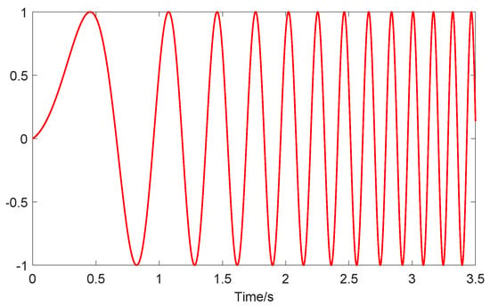
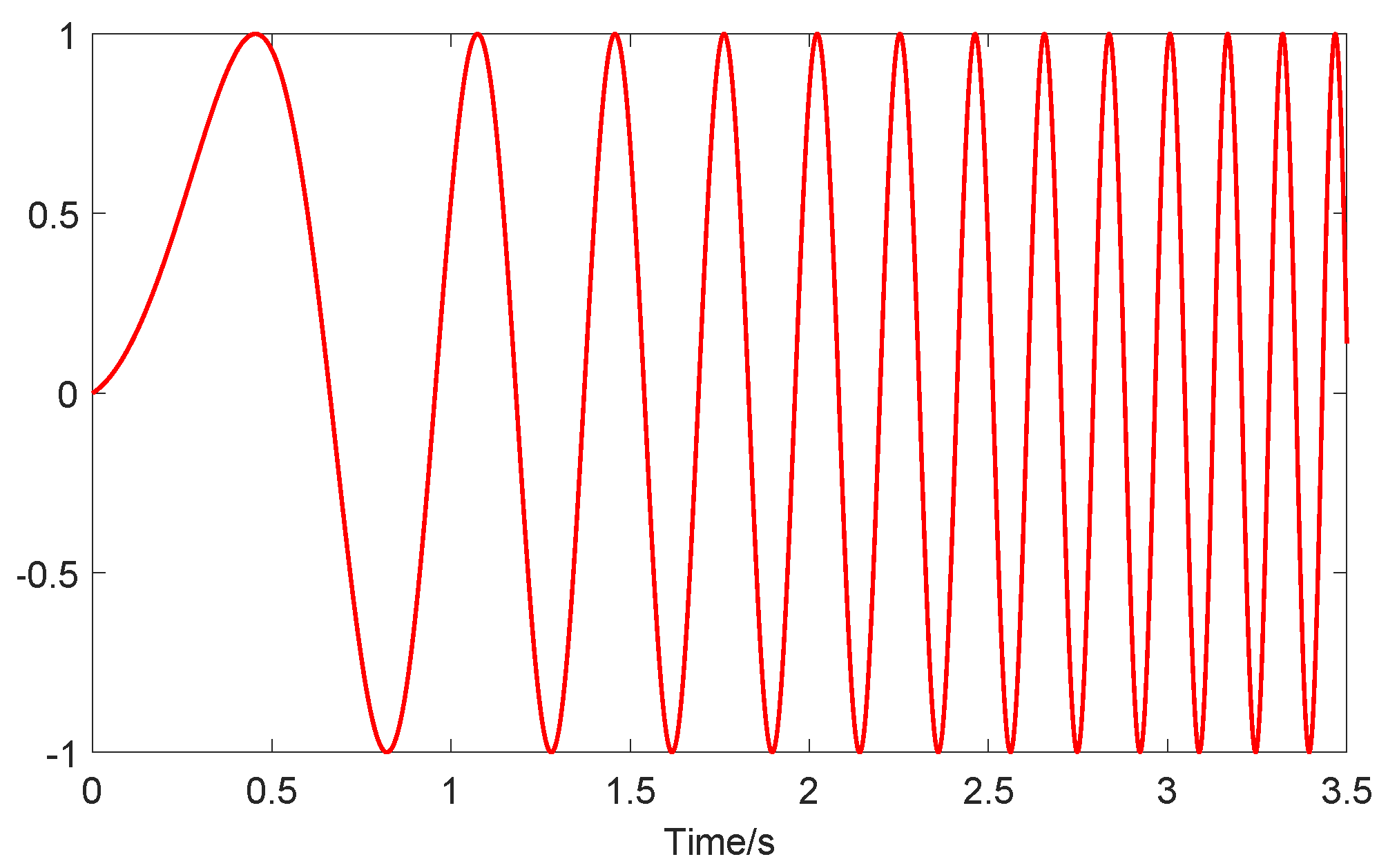
The setup of the simulations is as follows: to obtain the data snapshots at an equilibrium point of a fixed angle of attack. The sweep-frequency chirp signal is often used to excite modes in aeroelasticity identification [31]. As often used in some references [17], a chirp signal in Figure 2 is applied to the main-wing flap at one fixed angle of attack to excite the aeroelastic modes. The chirp signal of the control surface deflection has a magnitude of 1°, time duration of 3.5 s, and frequency components spanning from 0.1 Hz to 10 Hz in order to slightly perturb the equilibrium condition. The flexible wing is simulated with zero initial states, and the chirp signal is fed into the full-order nonlinear aeroelastic system to carry out simulations with a sampling rate of $T_s=0.001 \mathrm{s}$. The data snapshot of states and inputs are collected to conduct the data-driven LPV-ROM modeling algorithm, which has a data length of $N_d=3500$ and no pre-processing is needed for the p-DMD modeling.

Figure 2. Excitation input (deflection angle in degree) of a chirp signal with sweep frequency from 0.1 to 10 Hz.

4.1.1. Model Order and Polynomial Order Versus Modeling Accuracy

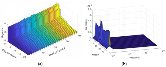
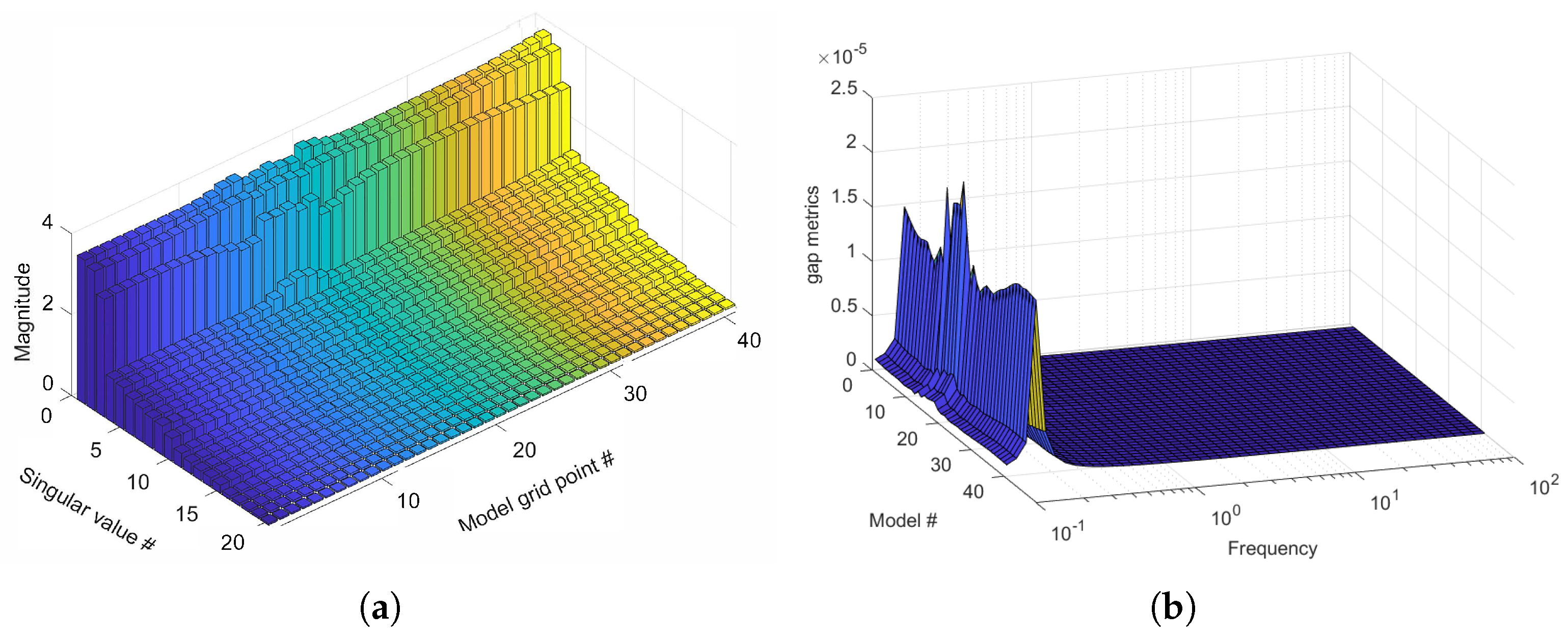
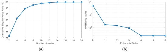
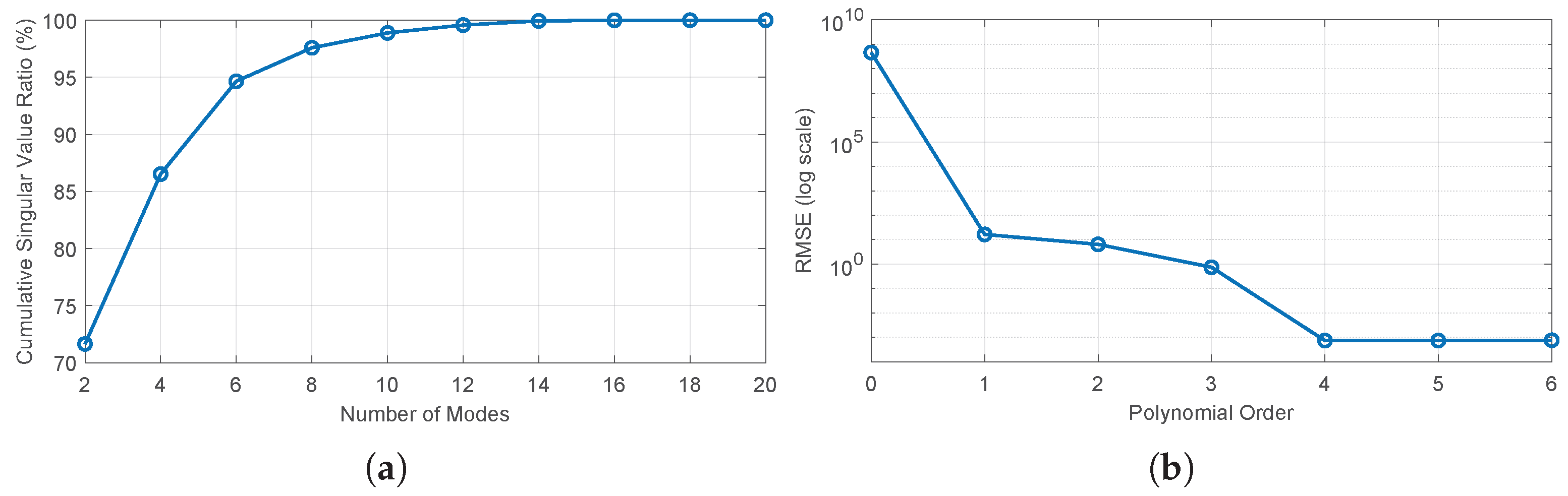
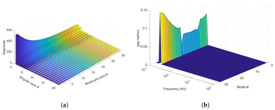
The p-DMD method is repeatedly applied at grid angle of attack, and the order of ROMs versus modeling accuracy is explored by evaluating the modeling accuracy against training data. The following results provide evaluations of the training-fit accuracy. The first 20 most significant singular values are plotted in Figure 3a. It can be seen that the first 12 singular values can retain over 99% of the summation of all singular values, and they are selected as the order of ROMs. Table 4 provides a summary of cumulative retained energy by different model orders of the most dominant singular values across different flight conditions. Figure 4 shows the cumulative singular values ratio using different model orders from 2 to 20. Note that most of the aeroelastic modes are in pairs, so the orders have increments of 2. In addition, there are 41 grid models at different angles of attack, and the sensitivity study reflects the averaged cumulative singular value ratios under different model orders. In addition, with the chosen model order of 12, the polynomial order is studied and plotted against the root mean square error (RMSE) of strains on the wing, which is expressed in log scale. The RMSE is computed by the formula $\mathrm{RMSE}=\sqrt{{\displaystyle \frac{1}{N}}{\sum }_{i=1}^N{\left(y_i-{\widehat{y}}_i\right)}^2}$, where $y_i$ is the reference value, ${\widehat{y}}_i$ is the predicted value, and N is the number of samples. With polynomial orders of 0–6, the RMSEs of all strains are $4.61\times {10}^8, 16.41, 6.44, 0.74, 7.41\times {10}^{-4},7.41\times {10}^{-4},$ and $7.41\times {10}^{-4}$. It can be seen that a polynomial order of 4 is the minimum needed to render accurate predictions. The polynomial order is selected as 4 to formulate LPV-ROM.

Figure 3. (a) Twenty largest singular values of grid models at fixed scheduling parameters; (b) v-gap metric surface of frequency responses at fixed models. A gap metric close to zero indicates that the two systems are dynamically similar. # indicates the index number.

Table 4. Cumulative retained energy (%) by singular values across 41 flight conditions (varying angles of attack) for flexible wing.

Retained Modes	Mean	Max	Min	Standard Deviation
2	72.35%	75.89%	64.93%	2.03%
4	87.32%	91.47%	85.44%	1.61%
6	94.87%	95.28%	91.06%	1.14%
8	96.65%	97.79%	95.71%	0.64%
10	98.80%	98.98%	98.67%	0.10%
12	99.51%	99.54%	99.44%	0.023%
14	99.79%	99.83%	99.73%	0.022%

Figure 4. (a) Sensitivity study of cumulative singular value ratios with different model orders averaged across 41 grid models; (b) sensitivity study of polynomial order versus RMSE of strains on a logarithmic scale.

v-gap metric is a distance measure in robust control theory to quantify closed-loop similarities between two linear systems [32]. With two systems $P_1$ and $P_2$, the Vinnicombe gap metric is used and computed as ${\delta }_{\nu }(P_1,P_2)={\max }_{\omega }{∥{\left(I+P_2{P}_2^{*}\right)}^{-1/2}(P_1-P_2){\left(I+P_1^{*}{P}_1\right)}^{-1/2}∥}_{\infty }$. The stabilizing feedback controller of system $P_1$ with stability margin $b_m$ will also stabilize system $P_2$ if ${\delta }_{\nu }$ is smaller than $b_m$. This measure is particularly useful in evaluating ROMs from the perspective of closed-loop systems, because it directly evaluates whether the ROMs preserve the feedback-control characteristics of the FOMs.

The v-gap metrics between the ROMs and linearized FOMs at fixed parameters are plotted in Figure 3b to evaluate the model accuracy of the ROMs. The gap metric indicates the distances between two systems and ranges between 0 and 1. A value close to zero indicates that FOM and ROM exhibit similar closed-loop characteristics, and the stabilizing controller of ROM can stabilize FOM [32]. Figure 3b shows that the maximum gap metric occurs around 0.1 Hz, and it has a very small value of the ${10}^{-5}$ level. The statistical summary of $\nu$-gap analyses is provided in Table 5. Therefore, the LPV-ROM model of order 12 can accurately capture the full-order model in the selected frequency range.

Table 5. Statistical summary of the $\nu$-gap metric across the flight envelope for flexible wing.

Model	$\mathit{\alpha }$	Mean	Max	Min	Standard Deviation
1	$-10°$	$5.80\times {10}^{-7}$	$1.50\times {10}^{-5}$	$6.65\times {10}^{-10}$	$2.18\times {10}^{-6}$
11	$-5°$	$5.01\times {10}^{-7}$	$1.30\times {10}^{-5}$	$5.69\times {10}^{-10}$	$1.89\times {10}^{-6}$
21	0°	$5.20\times {10}^{-7}$	$1.34\times {10}^{-5}$	$5.90\times {10}^{-10}$	$1.96\times {10}^{-6}$
31	$5°$	$5.67\times {10}^{-7}$	$1.47\times {10}^{-5}$	$6.49\times {10}^{-10}$	$2.14\times {10}^{-6}$
41	$10°$	$6.49\times {10}^{-7}$	$1.62\times {10}^{-5}$	$7.47\times {10}^{-10}$	$2.37\times {10}^{-6}$
All	$-10°$ to $10°$	$5.84\times {10}^{-7}$	$2.17\times {10}^{-5}$	$5.31\times {10}^{-10}$	$2.19\times {10}^{-6}$

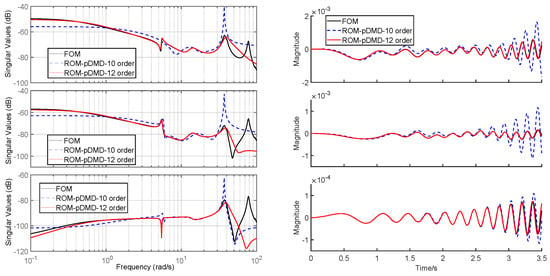
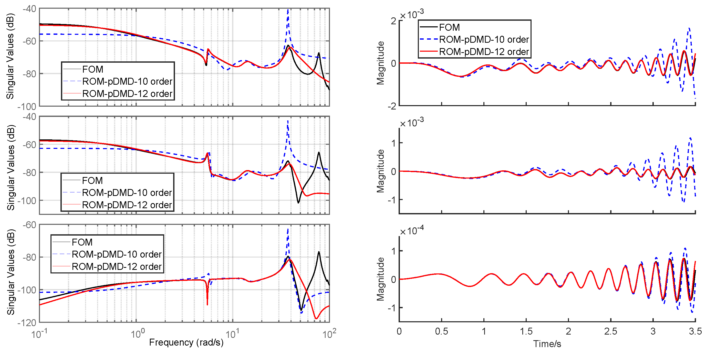
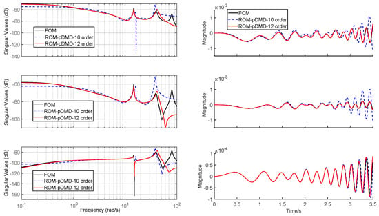
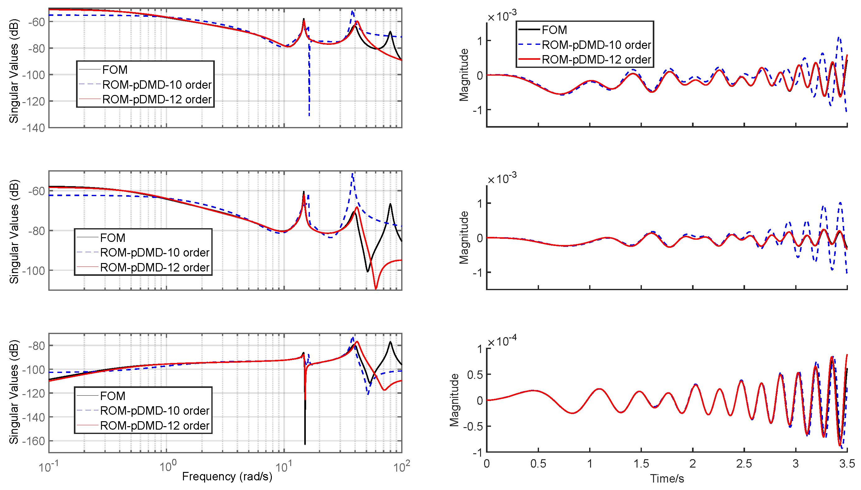
At angles of attack $\alpha$ equaling −10° and 0°, respectively, the time- and frequency-domain responses of linearized FOM, 10-order LPV-ROM, and 12-order LPV-ROM are compared in Figure 5 and Figure 6. Note that the plotted variables are the perturbed magnitudes from the trim points. It can be easily observed that the 10-order LPV-ROM has an obvious modeling error in the frequency range of concern, while the 12-order LPV-ROM model can capture the FOM in the frequency range of 0 rad/s to 40 rad/s (≈6.3 Hz). Therefore, the 12-order LPV-ROM is the “minimum order” model that can accurately describe the system’s dynamics.

Figure 5. Frequency responses (left column) and time responses (right column) of u to $y_1$ (top), $y_5$ (middle), and $y_{10}$ (bottom), with 10th- and 12th-order ROMs at the angle of attack $\alpha =-10°$.

Figure 6. Frequency responses (left column) and time responses (right column) of u to $y_1$ (top), $y_5$ (middle), and $y_{10}$ (bottom), with 10th- and 12th-order ROMs at the angle of attack $\alpha =0°$.

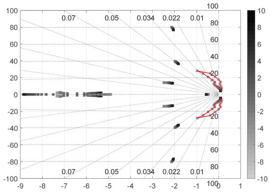
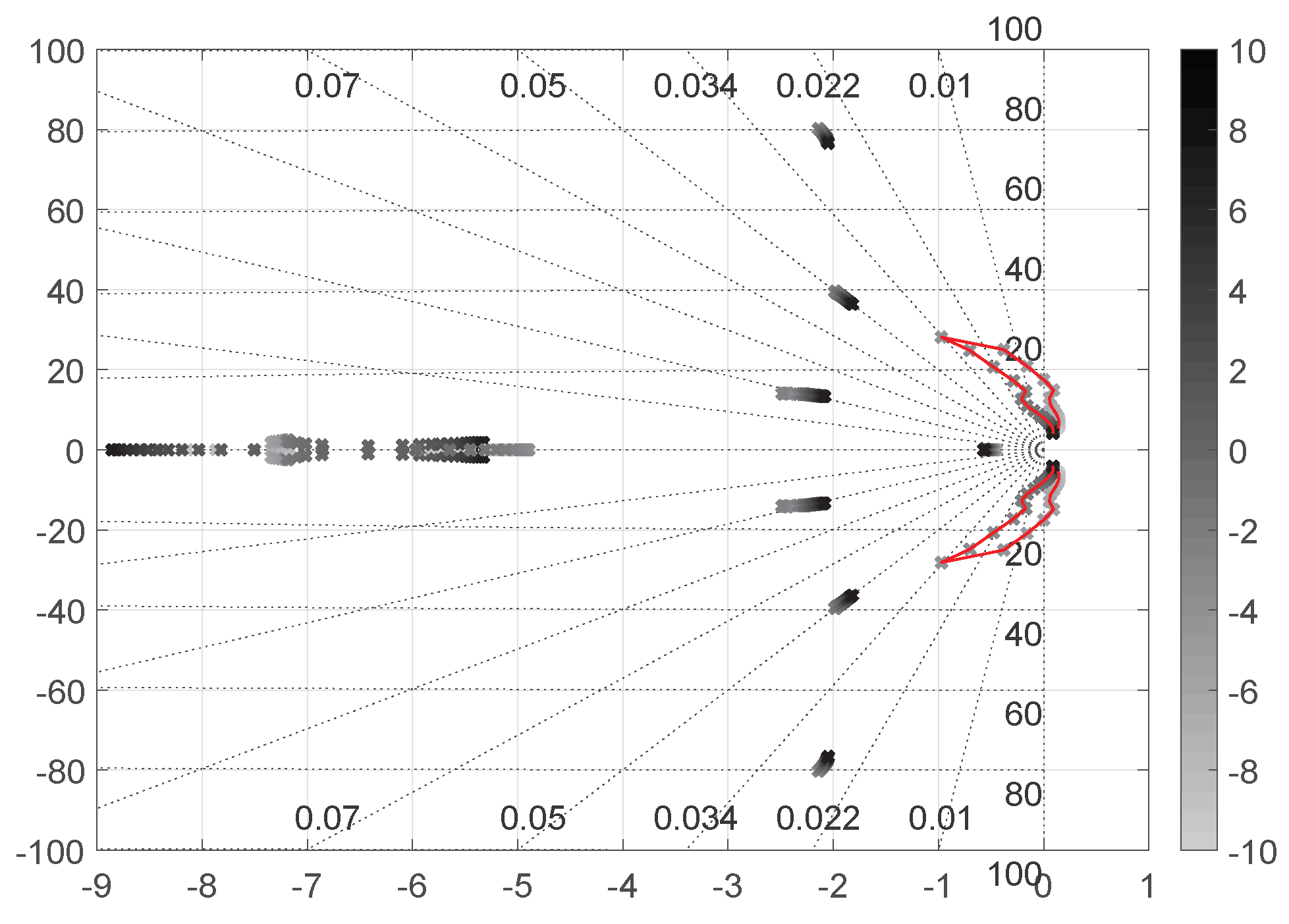
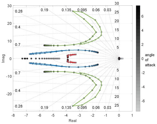
Moreover, it is necessary to note that the parameter-dependent reduced-order model is constructed using polynomial dependence on the scheduling parameter to approximate the nonlinear aeroelastic dynamics over a finite operating envelope. The validity of the approximation is therefore fundamentally associated with the range of scheduling parameters and structural deformation states represented in the training dataset. As shown in the root locus of Figure 7, polynomial dependence spans across unstable and stable regions of system dynamics. While polynomial dependence provides smooth interpolation across the trained stable and unstable operating regions, extrapolation beyond the sampled parameter range may introduce modeling errors or inaccurate modal trends.

Figure 7. Root loci of ROMs of slender wing at grid points of the angle of attack.

Beyond modeling accuracy, the reduced-order model provides improved computational efficiency over the full-order model. To compare computational times, the slender wing is simulated via 20-s open-loop simulations using a full-order model (140-order) and reduced-order model (12-order), and both models have a sampling rate of 0.001 s. Using an MSI Sword 15 AI12UE laptop (Intel Core i7-12650H, 40 GB RAM) to run simulations 10 times, the average time of each simulation is 0.0962 s for the FOM and 0.0141 s for the ROM. This demonstrates the greatly improved computational efficiency of the reduced-order models in open-loop simulations.

4.1.2. Comparisons Between p-DMD Modeling and Linearization-Based Modeling

In this section, the results from the authors’ previous work on linearization-based modeling are compared with data-driven p-DMD modeling. The nonlinear model in Equation (1) is linearized and reduced in order at grid angles of attack to obtain a series of LTI-FOM. The root loci of the ROMs are shown in Figure 7.

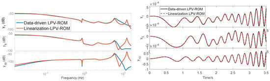
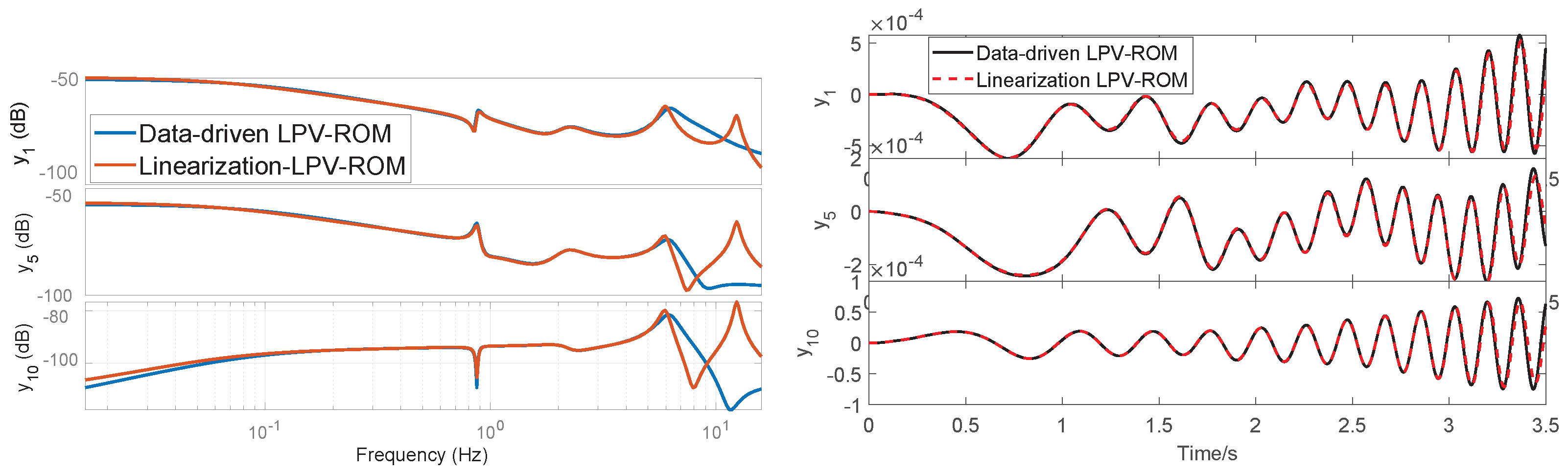
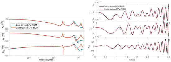
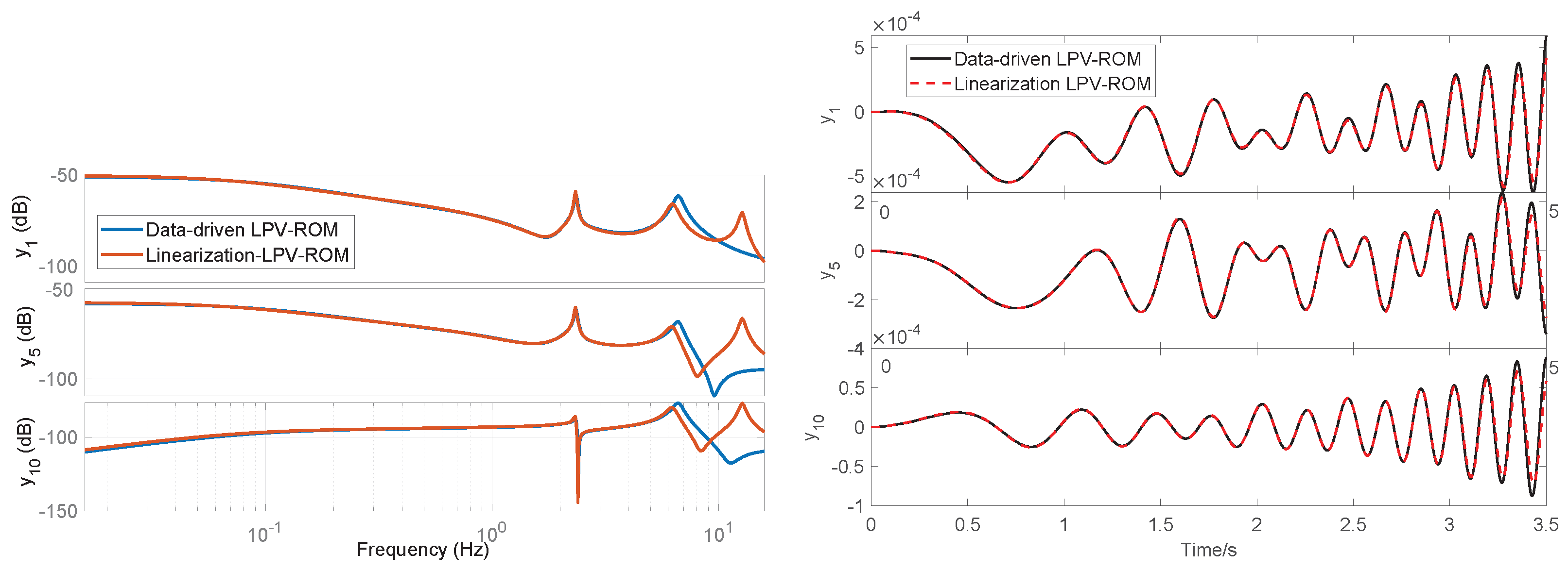
For reasonable comparisons, the equilibrium conditions at multiple angles of attacks are focused. The data snapshots are obtained by simulating the aeroelastic model at small perturbations of steady-state conditions using the chirp signal in Figure 2. Note that the dynamics responses of the nonlinear full-order model and the linearized full-order model have a difference with RMSEs of $1.14\times {10}^{-6},5.16\times {10}^{-7}$ and $3.37\times {10}^{-8}$ and RRMSEs of $0.402\%,0.435\%$, and $0.125\%$ for outputs $y_1, y_5$, and $y_{10}$. In other words, the linearized full-order model is almost identical to the full-order nonlinear model around the equilibrium point perturbed by the chirp signal; thus, only the responses of linearized models are displayed. The comparisons are plotted in Figure 8 and Figure 9, while the statistical summary is provided in Table 6. In the case of $\alpha =-10°$, the RMSEs of their differences are $3.74\times {10}^{-5},1.25\times {10}^{-5}$, and $5.89\times {10}^{-6}$, respectively, for $y_1,y_5$, and $y_{10}$. In the case of $\alpha =0°$, the RMSEs of their differences are $2.60\times {10}^{-5},1.28\times {10}^{-5}$, and $5.31\times {10}^{-6}$, respectively, for $y_1, y_5$, and $y_{10}$. The data-driven LPV-ROM is found to match the linearization-based LPV-ROM, verifying that the data-driven approach can capture the physical characteristics of aeroelasticity.

Figure 8. Comparison of frequency- and time-domain responses of data-driven ROMs and linearization-based ROMs at $\alpha =-10°$.

Figure 9. Comparison of frequency- and time-domain responses of data-driven ROMs and linearization-based ROMs at $\alpha =0°$.

Table 6. Error metrics for time-domain and frequency-domain response comparisons between the LPV-ROM and the linearized ROMs.

		Time Domain				Frequency Domain
Scenario	Output	RMSE	RRMSE	Max	Min	Max (dB)	Min (dB)
$\alpha =-10°$	$y_1$	3.74  $\times {10}^{-5}$	1.27%	2.66 $\times {10}^{-4}$	0	2.21	0
	$y_5$	1.25 $\times {10}^{-5}$	0.98%	7.61 $\times {10}^{-5}$	0	2.32	0.01
	$y_{10}$	5.89 $\times {10}^{-6}$	2.23%	3.88 $\times {10}^{-5}$	0	2.33	0
$\alpha =0°$	$y_1$	2.60 $\times {10}^{-5}$	0.94%	1.83 $\times {10}^{-4}$	0	2.65	0.01
	$y_5$	1.28 $\times {10}^{-5}$	0.94%	8.08 $\times {10}^{-5}$	0	2.69	0.02
	$y_{10}$	5.31 $\times {10}^{-6}$	2.02%	3.55 $\times {10}^{-5}$	0	1.72	0

It is worth mentioning the scenarios of $\alpha =-10°,+ 10°$; some eigenvalues have positive real parts (see root loci in Figure 7), indicating that the aeroelastic system is unstable at these angles of attack. In the linearization-based approach, the $\sigma$-shifted $H_2$ norm is calculated by shifting the eigenvalue by $\sigma$ to obtain a stable system [5]. However, the proposed p-DMD directly finds the dominant modes by analyzing the singular values of parametric data-trace matrices. The p-DMD approach can address the unstable dynamics.

To conclude this section, the p-DMD method can accurately capture the local dynamics of the highly flexible wing at a fixed angle of attack, and the model’s accuracy is verified with the well-established linearization-based approach in frequency- and time-domain simulations.

5. Numerical Study Case 2: Highly Flexible Aircraft

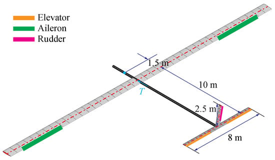
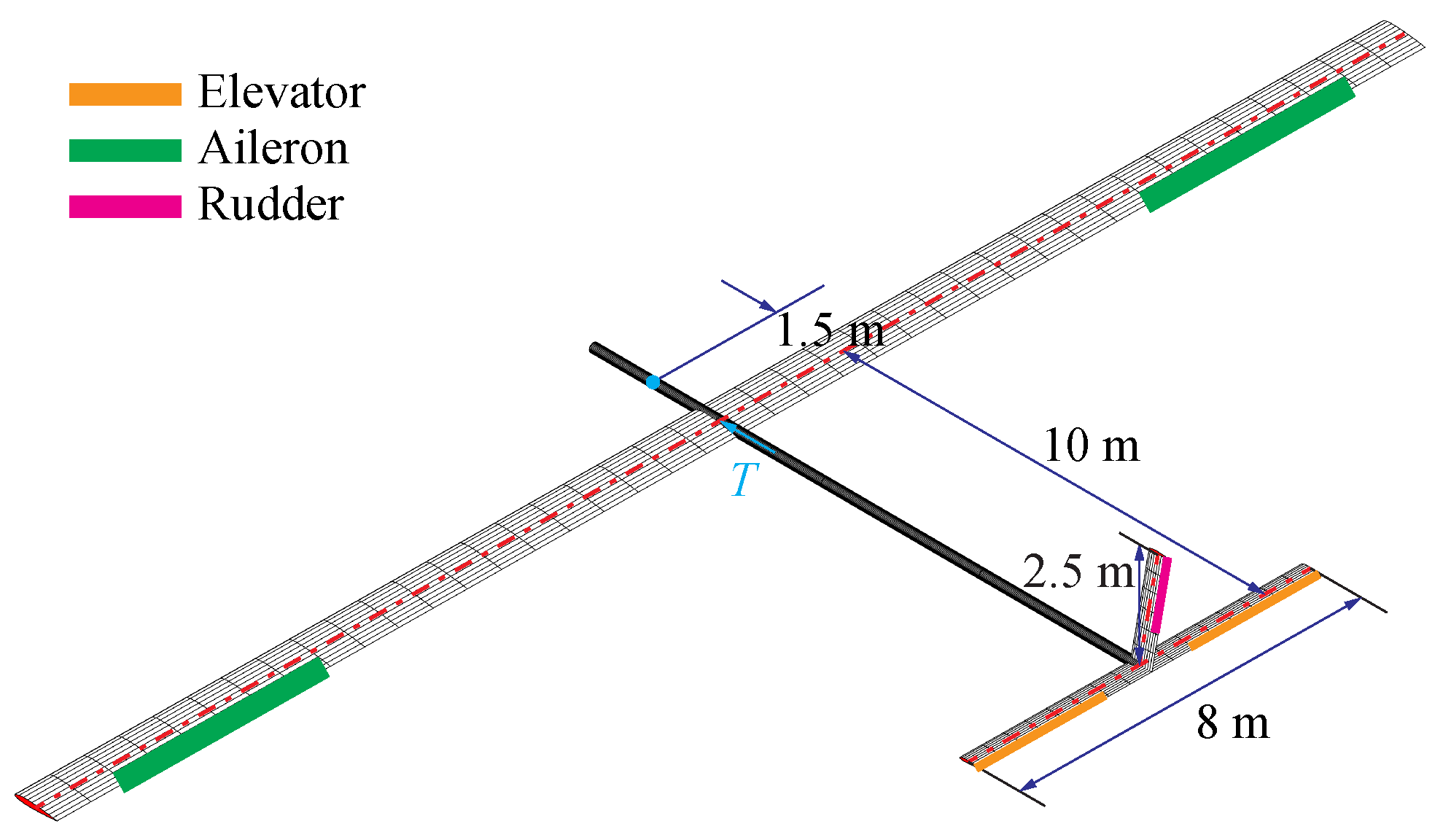
In this section, we study and show the results of data-driven modeling for a highly flexible aircraft with coupled elastic deformation and rigid-body motions. The aircraft is built based on the slender wing in Section 4, as shown in Figure 10. All members of the aircraft are modeled as slender beams. However, the body and tail members are rigidized, allowing one to focus on the high flexibility of the main wings. The chord length of the horizontal and vertical tails is 0.5 m, while their beam reference lines are defined at a quarter of the chord from the leading edge. There is no aerodynamics coupled on the body. Similarly to the main wing, trailing-edge control surfaces are also defined on the horizontal tail, from 25% to the full span. The flaps on the horizontal tail are used as elevators to trim the vehicle for level flight and to excite longitudinal motion.

Figure 10. Platform of flexible vehicle.

5.1. Fixed Scheduling Parameter (Angle of Attack)

In this section, we compare the p-DMD with the linearized FOM of flexible aircraft at fixed angles of attack. The results demonstrate the modeling capability of p-DMD for coupled rigid-body and vibration dynamics at equilibrium flight conditions.

In this simulation, the highly flexible aircraft is cruising in a freestream of $U_{\infty }=22$ m s⁻¹ at an altitude of 20,000 m. For LPV modeling, the body angle of attack at the origin of the body frame is used as the scheduling parameter. The LPV models span at grid angles of attack ranging from −7.5° to 7.5° with an increment of 0.5°. The total number of grid models is 31. The flexible vehicle model has 34 beam elements and three control inputs (control surfaces of the main wing deflect with the same angle, one elevator, and one thrust). The symmetric wing vibrations and longitudinal rigid-body motion are considered. Instead of being used as ailerons, the control surfaces on the main wing deflect symmetrically when excited. The FOM includes four strains, four strain rates, and six aerodynamic states for each beam element, in addition to six rigid-body velocities, four quaternions, and three inertial positions of the vehicle. Therefore, at a given angle of attack, the full-order A matrix is of dimension $471\times 471$, the B matrix is of dimension $471\times 3$, and the 26 outputs are selected as the out-of-plane bending strains on all main-wing elements (20 in total) plus longitudinal and vertical body velocities, pitch angle and rate, and longitudinal and vertical body positions.

At a fixed angle of attack, the chirp signal in Figure 2 is fed as the input perturbation of the main-wing flaps to excite the aeroelastic modes, and the data snapshots of states and inputs are collected to conduct the data-driven LPV-ROM modeling algorithm. The chirp signal consists of frequency components ranging from 0.1 Hz to 10 Hz. The full-order linearized aeroelastic system is also simulated at a sampling rate of $T_s=0.001 \mathrm{s}$. Therefore, the length of collected data for p-DMD model training is also $N_d=3500$. The evaluations of the training-fit accuracy have been performed. The 20 largest singular values of the state-kernel matrix are plotted in Figure 11a, among which the 12 largest singular values are determined to be able to capture over 95% accuracy of FOMs based on the cumulative singular values criteria. The model accuracy ${\eta }_r$ is computed as ${\eta }_r={\displaystyle \frac{{\sum }_{i=1}^r{\sigma }_i}{{\sum }_{i=1}^{n_x}{\sigma }_i}}$, where $\sigma$ is the singular values, r is the ROM order, and $n_x$ is the FOM order. Table 7 and Table 8 provide the cumulative retained energy by different numbers of singular values and the $\nu$-gap metrics across different flight conditions. The root loci of flexible vehicles at varying angles of attack are shown in Figure 12, which are obtained via model reduction from FOMs.

Figure 11. (a) Twenty largest singular values of flexible aircraft at fixed scheduling parameters. (b) v-gap metric surface of frequency responses of models at the grid angle of attack. Gap metric close to 0, meaning that two systems are similar.

Table 7. Cumulative retained energy (%) by singular values across the 31 different flight conditions of flexible aircraft.

Retained Modes	Mean	Max	Min	Std
2	65.25%	71.78%	63.12%	2.40%
4	89.78%	91.94%	87.92%	1.27%
6	94.30%	95.61%	93.23%	0.76%
8	97.37%	98.11%	96.76%	0.45%
10	99.07%	99.22%	98.97%	0.051%
12	99.58%	99.69%	99.52%	0.033%
14	99.84%	99.91%	99.79%	0.022%

Table 8. Statistical summary of the $\nu$-gap metric across the flight envelope for flexible aircraft.

Model	$\mathit{\alpha }$	Mean	Max	Min	Standard Deviation
1	−7.5°	$1.75\times {10}^{-3}$	$0.086$	$5.77\times {10}^{-8}$	$0.012$
11	−2.5°	$1.16\times {10}^{-3}$	$0.053$	$1.67\times {10}^{-7}$	$0.0076$
16	$-0°$	$1.17\times {10}^{-3}$	$0.056$	$5.51\times {10}^{-8}$	$0.0079$
21	2.5°	$1.81\times {10}^{-3}$	$0.084$	$2.64\times {10}^{-7}$	$0.012$
31	7.5°	$2.88\times {10}^{-3}$	$0.14$	$1.07\times {10}^{-7}$	$0.019$
All	−7.5° to 7.5°	$1.71\times {10}^{-3}$	$0.14$	$4.62\times {10}^{-8}$	$0.0115$

Figure 12. Root loci of ROMs of flexible aircraft at grid angles of attack.

The v-gap metric comparison between the LTI-ROMs and LPV-ROMs by applying p-DMD on flexible vehicles is plotted in Figure 11b. These gap metrics are close to 0 for most of the regime, indicating that the data-driven LPV-ROM can capture the local dynamics across the entire flight envelope and that the stabilizing controller designed based on ROM can stabilize the FOM.

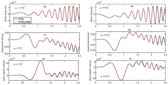
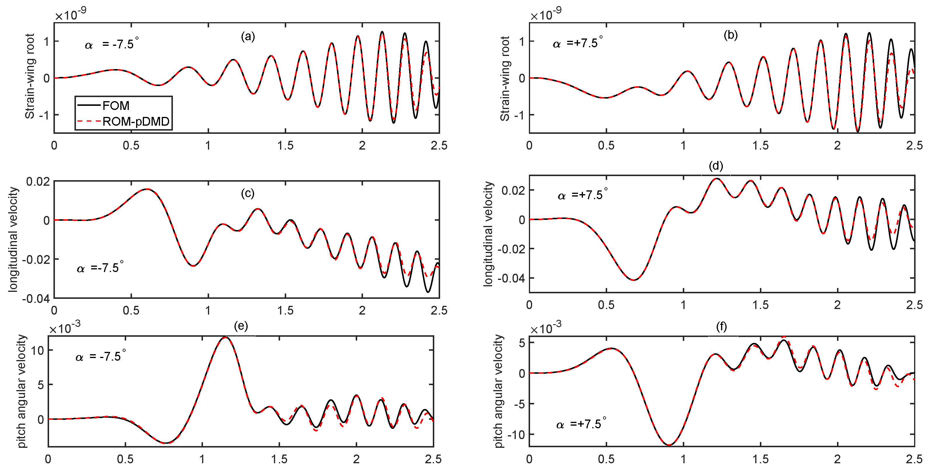
The time-domain responses of data-driven LPV-ROM and full-order linearized models are compared in Figure 13, and the statistical summary is shown in Table 9. The strain of the wing root, the longitudinal velocity, and the pitch rate all match with an error of less than 2%, as quantified by the relative root mean square error (RRMSE). The RRMSE is computed as $\mathrm{RRMSE}=\sqrt{{\displaystyle \frac{\frac{1}{N}{\sum }_{k=1}^N{(y_k-{\widehat{y}}_k)}^2}{\frac{1}{N}{\sum }_{k=1}^N{y}_k^2}}}\times 100\%$, where $y_k$ and ${\widehat{y}}_k$ denote the reference and predicted outputs, respectively. It is obvious that the p-DMD method can render an accurate LPV-ROM model at fixed equilibrium flight conditions. Note that at $\alpha =-7.5,7.5°$, the aeroelastic model becomes unstable (see Figure 12, one pair of eigenvalues has positive real parts), but the p-DMD can still render an accurate data-driven model. The frequency-domain response comparisons are omitted for the sake of the space limit.

Figure 13. Time-domain perturbation responses of LPV-ROM and FOM at angle of attack $\alpha =-7.5,+7.5°$. (a,b): Bending strains at wing root; (c,d): longitudinal velocity; (e,f): pitch rate.

Table 9. Error metrics for responses comparisons between LPV-ROM and the linearized FOMs.

Scenario	Output	RMSE	RRMSE	Max Error	Min Error
$\alpha =-7.5°$	Strain at wing root	7.51 × 10−10	1.53%	3.79 × 10−10	0
	Longitudinal velocity	1.42 × 10−3	0.99%	7.63 × 10−3	0
	Pitch rate	3.18 × 10−4	0.91%	1.27 × 10−3	0
$\alpha =+7.5°$	Strain at wing root	9.62 × 10−11	1.67%	5.20 × 10−10	0
	Longitudinal velocity	2.00 × 10−3	1.18%	1.12 × 10−2	0
	Pitch rate	3.41 × 10−4	0.84%	1.39 × 10−3	0

5.2. Varying Scheduling Parameter (Angle of Attack)

In this section, the capability to model aeroelasticity at varying angles of attack and non-equilibrium conditions is demonstrated. Note that the linearization-based approach and traditional DMD approach established for equilibrium conditions cannot handle this free-fly non-equilibrium case, and the time-domain responses of the LPV-ROM from p-DMD is compared against nonlinear full-order model.

The nonlinear equation of motion (Equation (1)) is numerically integrated in the time domain to obtain the vehicle’s nonlinear transient behavior. The nominal flight speed is still 22 m s⁻¹ and the altitude is 20,000 m. The simulation starts with a static operating condition, where the body pitch angle is ${\theta }_B=$ 2.14°, elevator deflection is ${\delta }_e=$ 2.57°, and thrust is $T=$ 51.07 N. A chirp signal with a magnitude of 5° and sweep frequency of 0.01–2 Hz is applied to the elevator to excite the rigid-body pitch motions and aeroelastic dynamics in such a frequency range. The simulation is conducted with a sampling time of 0.005 s, and the simulations are performed for 10 s. All the state and input data are collected without pre-processing, and the data length for training is $N_d=2000$. The scheduling parameter (angle of attack) is calculated in real time by $\alpha =-\arcsin ({\beta }_3/U_{\infty })$.

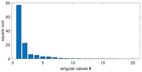
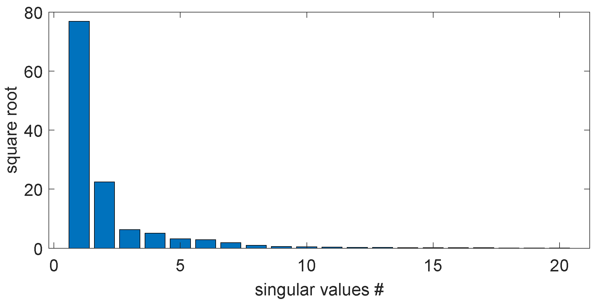
Note that the simulation is carried out to generate the snapshots of the full-order model in flight. For the same purpose, the snapshots can be obtained by collecting aircraft flight test data. Nonetheless, the collected data snapshots are applied with the p-DMD to obtain the data-driven LPV-ROM. The 20 largest singular values of the parametric data-trace matrix are plotted in Figure 14. The data-driven LPV-ROM is chosen to have the polynomial order of 4 and dimension of 12.

Figure 14. Square roots of 20 largest singular values of the parametric data-trace matrix. # indicates the index number.

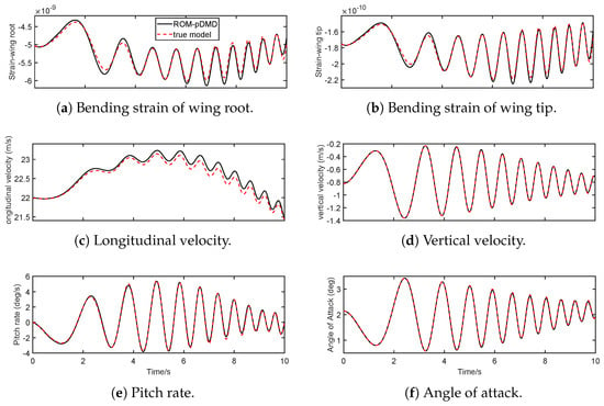
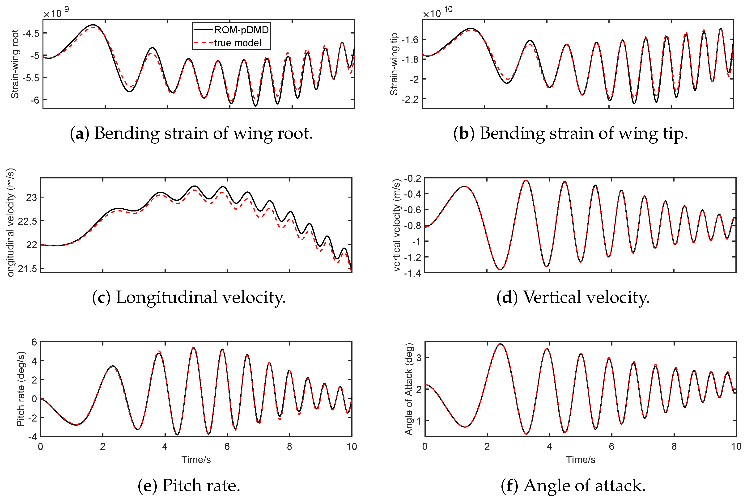
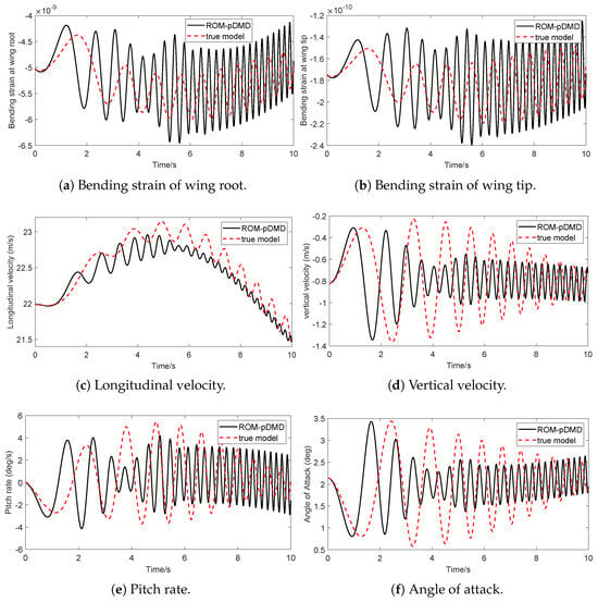
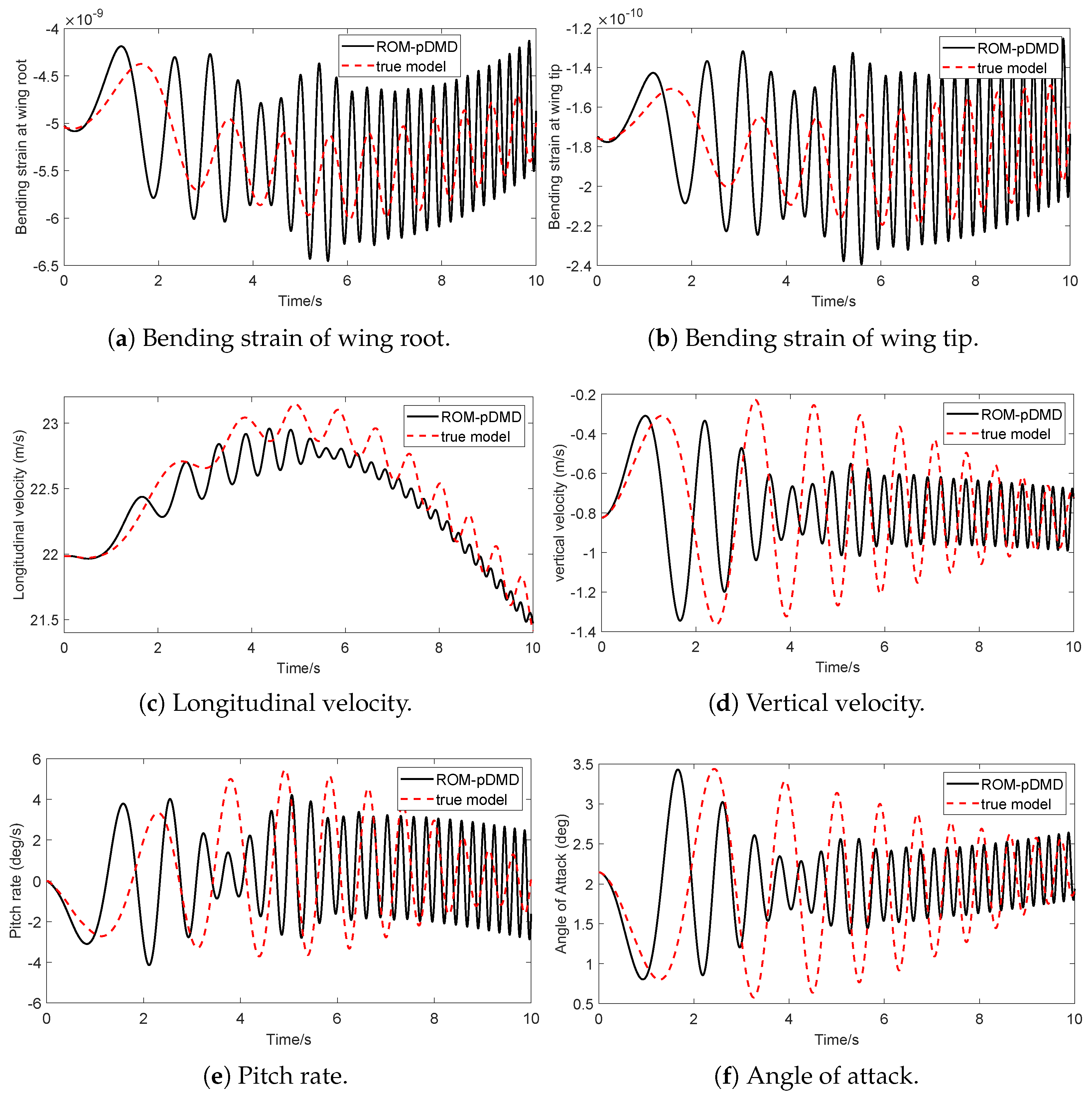
After that, the model accuracy of LPV-ROM is verified using other control inputs. There are two validations cases evaluated: (1) a chirp signal with a sweep frequency of 0.1–2 Hz within the frequency range of training data, with the results shown in Figure 15; (2) a 5 Hz sinusoidal signal beyond the frequency range of training data, with the results shown in Figure 16.

Figure 15. Time-domain responses of LPV-ROM and nonlinear FOM at non-equilibrium flight condition by chirp input of 0.1–2 Hz.

Figure 16. Time-domain responses of LPV-ROM and nonlinear FOM at non-equilibrium flight condition with sinusoidal input of 5 Hz.

First, one chirp signal with a magnitude of 5° and sweep frequency of 0.1–2 Hz is fed into the full-order nonlinear model and LPV-ROM, and their responses are compared. Figure 15 shows the vehicle’s time-domain elastic and rigid-body responses, with Table 10 showing the statistical metrics of the errors. First of all, the flight data show a dynamic flight with regard to rigid-body dynamics, and the vibrations of wings are excited by elevator deflections. The traditional linearization-based approach cannot address this case, since there is no trim/equilibrium in this dynamic flight. In addition, the LPV-ROM from p-DMD yields reasonably matching responses against the full-order nonlinear model with an averaged error of 2.7% quantified by the RRMSE. From the results, it is worth emphasizing that the bending strains and rigid-body velocities start from a non-zero initial condition and remain at a non-equilibrium flight condition. This demonstrates that the proposed p-DMD can address the non-equilibrium conditions. In addition, the angle of attack calculated from the two models’ responses matches accurately in Figure 15, which continuously varies between 0.5° and 3.5°. This study demonstrates that the proposed p-DMD can address the case of varying scheduling parameters. As stated in the novelties of this work, since no interpolation and linearization are used in the data-driven approach, the proposed method can derive parametric ROMs for flexible aircraft with large wing deformations and unsteady dynamics.

Table 10. Error metrics of the time-domain responses of the LPV-DMD model against the full-order nonlinear model.

Outputs	RMSE	RRMSE (%)	Max Error	Min Error
Strain at wing root	$8.23\times {10}^{-11}$	1.56%	$1.95\times {10}^{-10}$	$9.37\times {10}^{-14}$
Strain at wing tip	$2.74\times {10}^{-12}$	1.49%	$7.33\times {10}^{-12}$	$5.44\times {10}^{-16}$
Longitudinal vel.	$9.72\times {10}^{-2}$	0.43%	0.17	$9.58\times {10}^{-6}$
Vertical vel.	$5.70\times {10}^{-3}$	0.70%	0.014	$5.27\times {10}^{-6}$
Pitch rate	$0.127$	3.27%	0.33	$1.95\times {10}^{-4}$
Angle of attack	$0.021$	1.04%	$5.52\times {10}^{-2}$	$1.59\times {10}^{-5}$

To further evaluate the extrapolation capability out of the flight conditions in the training dataset, the validation of the ROM-pDMD model using a 5 Hz sinusoidal input with the same magnitude, a frequency outside the training dataset, is performed and presented in Figure 16. The results reveal significant discrepancies between the reduced-order approximation and the true physics-based model. While the ROM-pDMD initially tracks the phase and magnitude of variables, such as vertical velocity and angle of attack for the first second, it quickly diverges into high-frequency oscillations that do not align with the true model’s behavior. These results suggest that while the ROM may be effective within its training envelope, its predictive accuracy degrades under out-of-scope dynamic inputs, demonstrating the inherited limitations in extrapolation outside the scope of the training dataset.

6. Predictive Control of Flexible Wing Using p-DMD Model

In this section, a model predictive control (MPC) framework is developed to actively suppress the vibrations for the flexible cantilever wing based on the reduced-order LPV derived using p-DMD in Section 4. After one obtains the p-DMD model, the MPC computes the control sequence by solving the following finite-horizon quadratic program at each time step:

$$\begin{array}{c}\hfill \begin{array}{cc}\hfill {\displaystyle \underset{\mathbf{u}}{min}}{\displaystyle \underset{k=0}{\sum ^{N-1}}}& {\mathbf{y}}_k^T\mathbf{Q}{\mathbf{y}}_k+{\mathbf{u}}_k^T\mathbf{R}{\mathbf{u}}_k\hfill \\ \hfill s.t.{\mathbf{z}}_{k+1}& ={\mathbf{A}}_r\left({\theta }_k\right){\mathbf{z}}_k+{\mathbf{B}}_r\left({\theta }_k\right){\mathbf{u}}_k\hfill \\ \hfill {\mathbf{y}}_k& ={\mathbf{C}}_r{\mathbf{z}}_k\hfill \\ \hfill {\mathbf{u}}_{\min }& \le \mathbf{u}\le {\mathbf{u}}_{\max }\hfill \end{array}\end{array}$$

(22)

where ${\mathbf{z}}_k,{\mathbf{u}}_k,$ and ${\mathbf{y}}_{\mathbf{k}}$ denote states, control inputs, and outputs of the LPV-ROM at discrete-time step k. ${\theta }_k$ is the scheduling parameter of the angle of attack at time step k. The weighing matrices $\mathbf{Q}$ and $\mathbf{R}$ penalize the bending strains and the control inputs, respectively. In this study, the system’s outputs are defined as the out-of-plane bending strains of all ten wing elements, which capture the structural responses. The control input is the flap deflection angle that is used to actively suppress the bending strains. ${\mathbf{u}}_{\min }$ and ${\mathbf{u}}_{\max }$ are the bounds for the control inputs, which are set as ${\mathbf{u}}_{\min }=-20°$ and ${\mathbf{u}}_{\max }=20°$.

The discrete-time LPV-ROM is obtained using a sampling rate of $T_s=0.001$ s, while the MPC controller operates at a slower rate of 0.01 s to reduce computational demand for the consideration of real-time implementation. At each time step, the optimization problem is solved over a prediction horizon of 20, and only the first control input is applied to the full-order nonlinear model in a receding-horizon manner. The weighting matrix R is set as the identity matrix, and Q is set as $Q=\mathrm{diag}(2\times {10}^7{\mathbf{I}}_8,2\times {10}^8{\mathbf{I}}_2)$ to weigh more on wing tips. The resulting closed-loop responses are then compared against a baseline case without the active control input.

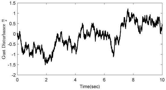
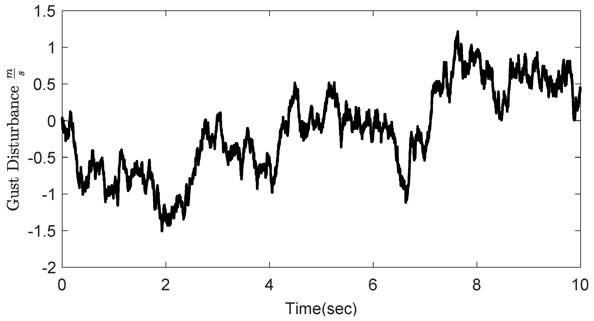
A flexible wing is simulated with perturbations around the steady state at an angle of attack of $-2°$ and $U_{\infty }=22$ m/s and an altitude of 20,000 m. A Dryden gust is applied to the full-order nonlinear flexible wing to excite the vibrations on the wing, which is plotted in Figure 17. The Dryden gust is generated by following military specification MIL-F-8785C and filtering Gaussian white noise through a transfer function $H_w\left(s\right)={\sigma }_w\sqrt{{\displaystyle \frac{L_w}{\pi U_{\infty }}}}{\displaystyle \frac{1+\sqrt{3}\frac{L_w}{U_{\infty }}s}{{\left(1+\frac{L_w}{U_{\infty }}s\right)}^2}}$. s is the Laplace variable, $U_{\infty }$ is airspeed, $L_w$ is the gust’s scale length, and ${\sigma }_w$ is the gust’s density, both of which are determined by the altitude. The specifications of the gust model are selected as follows: zero-mean unit energy white noise filtered by a filter with a gust length of $L_w=533$ m and severe gust density of ${\sigma }_w=6$ m/s. The vertical gust velocity $w_g\left(t\right)$ is uniformly applied on the wing’s surface and perturbs the effective angle of attack at each wing section. The gust-induced angle-of-attack increment is ${\alpha }_g\left(t\right)=\arctan {\displaystyle \frac{w_g\left(t\right)}{U_{\infty }}}\approx {\displaystyle \frac{w_g\left(t\right)}{U_{\infty }}}$ for small angles. The gust’s disturbance enters the system as external disturbance to the aeroelastic dynamics, which is not known to the MPC controller. Note that the full states of the flexible wing are not needed in the MPC once the ROM is obtained, and the scheduling parameter ${\theta }_k$, bending strain ${\mathbf{y}}_k$, and ROM state ${\mathbf{z}}_k$ are needed for feedback, which are available in the simulation environment. The states ${\mathbf{z}}_k$ are the projected ROM states and propagate from zero initial states.

Figure 17. Profile of the Dryden gust disturbances to excite the flexible wing.

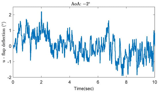
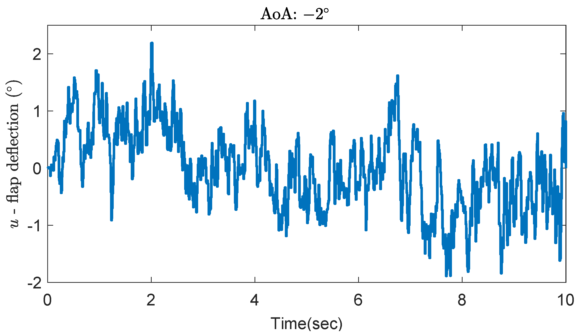
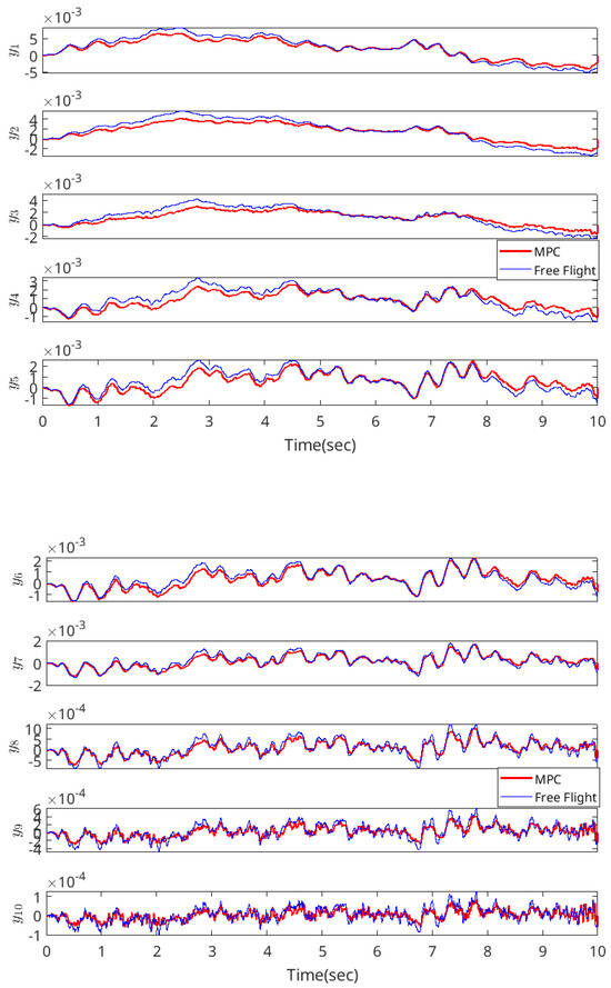
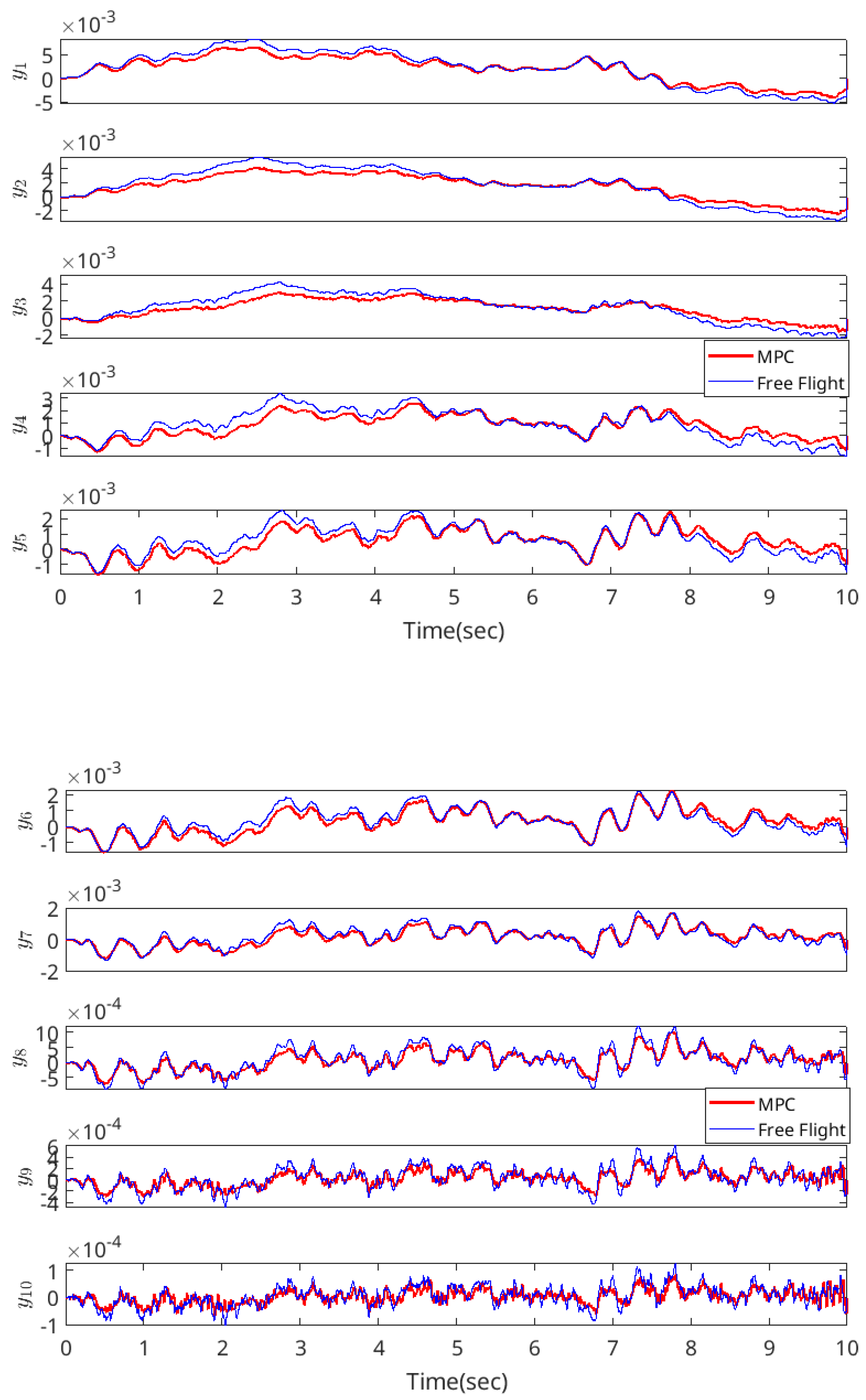
To solve the quadratic programming formulated by the MPC, the SeDuMi solver [33] is used in the simulation. The control sequence obtained by solving the receding-horizon optimization is plotted in Figure 18. Flap deflection ranges between +2.2° and −1.9°, with total control energy around 6.5 deg²·s. Figure 19 compares the MPC-controlled response with the baseline case in which no active control input is applied. The analysis focuses on the out-of-plane bending strains from all ten wing elements—ranging from the wing root $y_1$ to the wing tip $y_{10}$—which are the primary indicators of vibration suppression. It is important to emphasize that the MPC formulation does not explicitly incorporate gust disturbances in the optimization process. Under the specific gust profile as shown in Figure 17, the RMSEs of the bending strains in MPC-controlled and uncontrolled scenarios are summarized and compared in Table 11. It can be seen that the active control designed based on the data-driven aeroelastic model can lead to improvements on all wing elements from the wing root to the wing tip, with an average of 18.34%. The peak reduction of each strain by the MPC is 21%, 25%, 28%, 34%, and 25% for $y_1$ to $y_5$ and 20%, 18%, 18%, 23%, and 30% for $y_6$ to $y_{10}$, respectively. The control input is plotted in Figure 18. The total energy is calculated as 6.83 deg² × s, and its maximum absolute angle is around 2.16°.

Figure 18. Control input to actively suppress the vibration.

Figure 19. Comparison of time-domain bending strain responses for the MPC-controlled and uncontrolled systems.

Table 11. Comparisons of RMSEs and peak reductions for bending strain responses under uncontrolled and controlled conditions.

Strain	RMSE			Peak Reduction	Strain	RMSE			Peak Reduction
	Unctrl.	Controlled	$\Delta \%$			Unctrl.	Controlled	$\Delta \%$
$y_1$	0.4314	0.3523	18.4%	21%	$y_6$	0.0865	0.0823	5.0%	20%
$y_2$	0.3004	0.2353	21.7%	25%	$y_7$	0.0643	0.0582	9.6%	18%
$y_3$	0.2078	0.1605	22.7%	28%	$y_8$	0.0414	0.0335	19.0%	18%
$y_4$	0.1479	0.1211	18.1%	34%	$y_9$	0.0192	0.0137	28.4%	23%
$y_5$	0.1113	0.1009	9.4%	25%	$y_{10}$	0.0037	0.0025	30.8%	30%

Although this study focuses on the feasibility of reduced-order modeling and its usage in active vibration controller design, the practical implementation is discussed. For the 12th-order ROM with a prediction horizon of $N=20$ and control horizon of 1, the simulation is performed by MSI Sword 15 AI12UE laptop (Intel Core i7-12650H, 40 GB RAM) with a time duration of 10 s and MPC sampling rate of 10 ms. The average computation time per step was 29.5 ms, with a worst-case time of 290 ms. Therefore, the current implementation does not achieve real-time performance on this hardware. Several practical strategies can close this gap. First, replacing SeDuMi with a solver designed specifically for MPC can significantly reduce solve times. For example, OSQP [34] and HPIPM [35] routinely achieve sub-millisecond solve times for problems of this size. Second, this study does not consider the time constant of the actuator. Therefore, reducing the prediction horizon and choosing proper control sample times based on the actuation time constant should be considered in the practical implementation of controllers.

The reduced-order model is used in predictive control to actively suppress vibrations, and it can also be used to develop other control methods with reduced computations than full-order models: for example, LQR/LQG control. Considering model uncertainty by model reduction, robust control techniques ($\mu$ synthesis or $H_{\infty }$ control) can be designed based on the reduced-order model of flexible wings to achieve robust stability and robust performance with model uncertainty; see the authors’ previous works [36].

7. Conclusions

This paper presented a data-driven approach for generating accurate linear parameter-varying reduced-order models (LPV-ROMs) and predictive control regarding the nonlinear aeroelasticity and flight dynamics of highly flexible aircraft. This method encoded the nonlinear dynamics of highly flexible aircraft into a parametric data-trace matrix and performed parametric dynamic mode decomposition (p-DMD) to render LPV-ROMs.

Both the fixed and varying scheduling parameter scenarios could be addressed by the p-DMD modeling. The method was applied and verified with a highly flexible cantilever wing and a complete free-flight aircraft. Local modeling accuracy with fixed scheduling parameters was verified by cross-validation with the linearized model. In addition, modeling accuracy was verified by comparing it with the nonlinear full-order model regarding the time-domain responses in transient flight conditions. With the results of predictive control using the LPV-ROM from the p-DMD of flexible wings, this method is demonstrated by numerical simulations with the capability of directly using data to develop accurate models and control for flexible wing.

Future works include parametric modeling with noisy measurements of data snapshots and partially measurable states in experiments, extensions to multi-dimensional scheduling parameter cases, and the development of a parameter-dependent projection basis across varying flight conditions. In addition, the proposed method requires experimental validations using real flight data and is verified in real-time flight control to further demonstrate its feasibility.

References

- van Shoor, M.C.; Zerweckh, S.H.; von Flotow, A.H. Aeroelastic Stability and Control of a Highly Flexible Aircraft. In Proceedings of the 30th AIAA Structures, Structural Dynamics and Materials Conference, Mobile, AL, USA, 3–5 April 1989. [Google Scholar]
- Barker, J.M.; Balas, G.J. Comparing Linear Parameter-Varying Gain-Scheduled Control Techniques for Active Flutter Suppression. J. Guid. Control Dyn. 2000, 23, 948–955. [Google Scholar] [CrossRef] [Scilit]
- He, T.; Su, W. Robust Control of Gust-Induced Vibration of Highly Flexible Aircraft. Aerosp. Sci. Technol. 2023, 143, 108703. [Google Scholar] [CrossRef] [Scilit]
- He, T.; Zhu, G.; Swei, S.S.M.; Su, W. Smooth-Switching LPV Control for Vibration Suppression of a Flexible Airplane Wing. Aerosp. Sci. Technol. 2019, 84, 895–903. [Google Scholar] [CrossRef] [Scilit]
- Al-Jiboory, A.K.; Zhu, G.; Swei, S.S.M.; Su, W.; Nguyen, N.T. LPV Modeling of a Flexible Wing Aircraft Using Modal Alignment and Adaptive Gridding Methods. Aerosp. Sci. Technol. 2017, 66, 92–102. [Google Scholar] [CrossRef] [Scilit]
- Shu, J.I.; Wang, Y.; Krolick, W.C.; Pant, K. Parametric Aeroelastic Reduced-Order Model with State-Consistence Enforcement. AIAA J. 2023, 61, 1109–1128. [Google Scholar] [CrossRef] [Scilit]
- Fonzi, N.; Brunton, S.L.; Fasel, U. Data-Driven Nonlinear Aeroelastic Models of Morphing Wings for Control. Proc. R. Soc. A 2020, 476, 20200079. [Google Scholar] [CrossRef] [Scilit] [PubMed]
- Li, K.; Kou, J.; Zhang, W. Deep Neural Network for Unsteady Aerodynamic and Aeroelastic Modeling across Multiple Mach Numbers. Nonlinear Dyn. 2019, 96, 2157–2177. [Google Scholar] [CrossRef] [Scilit]
- Timme, S.; Marques, S.; Badcock, K. Transonic Aeroelastic Stability Analysis Using a Kriging-Based Schur Complement Formulation. AIAA J. 2011, 49, 1202–1213. [Google Scholar] [CrossRef] [Scilit]
- Juang, J.N.; Pappa, R.S. An Eigensystem Realization Algorithm for Modal Parameter Identification and Model Reduction. J. Guid. Control Dyn. 1985, 8, 620–627. [Google Scholar] [CrossRef] [Scilit] [PubMed]
- Zhang, W.; Ye, Z. Reduced-Order-Model-Based Flutter Analysis at High Angle of Attack. J. Aircr. 2007, 44, 2086–2089. [Google Scholar] [CrossRef] [Scilit]
- Zhang, W.; Ye, Z.; Zhang, C. Aeroservoelastic Analysis for Transonic Missile Based on Computational Fluid Dynamics. J. Aircr. 2009, 46, 2178–2183. [Google Scholar] [CrossRef] [Scilit]
- Lumley, J.L. The Structure of Inhomogeneous Turbulent Flows. In Atmospheric Turbulence and Radio Wave Propagation; Nauka: Moscow, Russia, 1967; pp. 166–178. [Google Scholar]
- Berkooz, G.; Holmes, P.; Lumley, J.L. The Proper Orthogonal Decomposition in the Analysis of Turbulent Flows. Annu. Rev. Fluid Mech. 1993, 25, 539–575. [Google Scholar] [CrossRef]
- Brunton, S.L.; Proctor, J.L.; Kutz, J.N. Discovering Governing Equations from Data by Sparse Identification of Nonlinear Dynamical Systems. Proc. Natl. Acad. Sci. USA 2016, 113, 3932–3937. [Google Scholar] [CrossRef] [Scilit]
- Kaiser, E.; Kutz, J.N.; Brunton, S.L. Sparse Identification of Nonlinear Dynamics for Model Predictive Control in the Low-Data Limit. Proc. R. Soc. A 2018, 474, 20180335. [Google Scholar] [CrossRef] [Scilit] [PubMed]
- Iannelli, A.; Fasel, U.; Smith, R.S. The Balanced Mode Decomposition Algorithm for Data-Driven LPV Low-Order Models of Aeroservoelastic Systems. Aerosp. Sci. Technol. 2021, 115, 106821. [Google Scholar] [CrossRef] [Scilit]
- Benner, P.; Gugercin, S.; Willcox, K. A Survey of Projection-Based Model Reduction Methods for Parametric Dynamical Systems. SIAM Rev. 2015, 57, 483–531. [Google Scholar] [CrossRef] [Scilit]
- Goizueta, N.; Wynn, A.; Palacios, R. Adaptive Sampling for Interpolation of Reduced-Order Aeroelastic Systems. AIAA J. 2022, 60, 6183–6202. [Google Scholar] [CrossRef] [Scilit]
- Willcox, K. Unsteady flow sensing and estimation via the gappy proper orthogonal decomposition. Comput. Fluids 2006, 35, 208–226. [Google Scholar] [CrossRef] [Scilit]
- Chaturantabut, S.; Sorensen, D.C. Nonlinear model reduction via discrete empirical interpolation. SIAM J. Sci. Comput. 2010, 32, 2737–2764. [Google Scholar] [CrossRef] [Scilit]
- Palacios, R.; Murua, J.; Cook, R. Structural and Aerodynamic Models in Nonlinear Flight Dynamics of Very Flexible Aircraft. AIAA J. 2010, 48, 2648–2659. [Google Scholar] [CrossRef] [Scilit]
- Peters, D.A.; Johnson, M.J. Finite-State Airloads for Deformable Airfoils on Fixed and Rotating Wings. In Proceedings of the Symposium on Aeroelasticity and Fluid/Structure Interaction; ASME Winter Annual Meeting; Friedmann, P.P., Chang, J.C.I., Eds.; American Society of Mechanical Engineers: New York, NY, USA, 1994; Volume AD-44, pp. 1–28. [Google Scholar]
- Peters, D.A.; Karunamoorthy, S.; Cao, W.M. Finite State Induced Flow Models Part I: Two-Dimensional Thin Airfoil. J. Aircr. 1995, 32, 313–322. [Google Scholar] [CrossRef] [Scilit]
- Peters, D.A.; He, C.J. Finite State Induced Flow Models Part II: Three-Dimensional Rotor Disk. J. Aircr. 1995, 32, 323–333. [Google Scholar] [CrossRef] [Scilit]
- Shearer, C.M.; Cesnik, C.E.S. Nonlinear Flight Dynamics of Very Flexible Aircraft. J. Aircr. 2007, 44, 1528–1545. [Google Scholar] [CrossRef] [Scilit]
- Su, W.; Cesnik, C.E.S. Nonlinear Aeroelasticity of a Very Flexible Blended-Wing-Body Aircraft. J. Aircr. 2010, 47, 1539–1553. [Google Scholar] [CrossRef] [Scilit]
- Su, W.; Cesnik, C.E.S. Dynamic Response of Highly Flexible Flying Wings. AIAA J. 2011, 49, 324–339. [Google Scholar] [CrossRef] [Scilit]
- Annoni, J.; Seiler, P. A method to construct reduced-order parameter-varying models. Int. J. Robust. Nonlinear Control 2017, 27, 582–597. [Google Scholar] [CrossRef] [Scilit]
- Patil, M.J.; Hodges, D.H.; Cesnik, C.E.S. Nonlinear Aeroelasticity and Flight Dynamics of High-Altitude Long-Endurance Aircraft. J. Aircr. 2001, 38, 88–94. [Google Scholar] [CrossRef] [Scilit] [PubMed]
- Kukreja, S.L.; Brenner, M.J. Nonlinear Aeroelastic System Identification with Application to Experimental Data. J. Guid. Control Dyn. 2006, 29, 374–381. [Google Scholar] [CrossRef] [Scilit]
- Zhou, K.; Doyle, J.C. Essentials of Robust Control; Prentice Hall: Upper Saddle River, NJ, USA, 1998; Volume 104. [Google Scholar]
- Sturm, J.F. Using SeDuMi 1.02, a MATLAB toolbox for optimization over symmetric cones. Optim. Methods Softw. 1999, 11, 625–653. [Google Scholar] [CrossRef] [Scilit]
- Stellato, B.; Banjac, G.; Goulart, P.; Bemporad, A.; Boyd, S. OSQP: An Operator Splitting Solver for Quadratic Programs. In 2018 UKACC 12th International Conference on Control (CONTROL); IEEE: New York, NY, USA, 2018; p. 339. [Google Scholar] [CrossRef] [Scilit]
- Frison, G.; Diehl, M. HPIPM: A high-performance quadratic programming framework for model predictive control. IFAC-PapersOnLine 2020, 53, 6563–6569. [Google Scholar] [CrossRef] [Scilit]
- He, T.; Al-Jiboory, A.K.; Zhu, G.G.; Swei, S.S.-M.; Su, W. Application of ICC LPV control to a blended-wing-body airplane with guaranteed H∞ performance. Aerosp. Sci. Technol. 2018, 81, 88–98. [Google Scholar] [CrossRef] [Scilit]
Disclaimer/Publisher’s Note: The statements, opinions and data contained in all publications are solely those of the individual author(s) and contributor(s) and not of MDPI and/or the editor(s). MDPI and/or the editor(s) disclaim responsibility for any injury to people or property resulting from any ideas, methods, instructions or products referred to in the content. |
© 2026 by the authors. Licensee MDPI, Basel, Switzerland. This article is an open access article distributed under the terms and conditions of the Creative Commons Attribution (CC BY) license.