


Abstract
To advance research in multi-agent reinforcement learning (MARL) for pursuit–evasion scenarios, this paper introduces a novel algorithm called Expert Knowledge and Opponent Modeling Multi-UAV Deep Deterministic Policy Gradient (EO-MADDPG). EO-MADDPG consists of two key components: the integration of expert knowledge and real-time sampled data and the prediction of evader UAV actions. The expert knowledge includes a multi-UAV formation control algorithm and an encirclement strategy, which incorporates consensus algorithms and Apollonius circle guidance. Additionally, the network-training framework is optimized by integrating information about opponent actions under a fixed policy for improved prediction accuracy. The experiments focus on three vs. one and three vs. two scenarios, where pursuer UAVs utilize EO-MADDPG and evader UAVs follow fixed policies with Gaussian perturbations. Experimental results show that EO-MADDPG achieves success rates of 99.9 ± 0.3% and 97.5 ± 1.4% (mean ± std over five seeds) in three vs. one and three vs. two pursuit–evasion simulations, respectively, outperforming the baseline MADDPG (72.7 ± 6.0% and 64.4 ± 34.4%). Ablation studies and cooperative landmark tasks further demonstrate improved training stability and interpretability.
1. Introduction
The pursuit–evasion problem is an important problem in multi-agent reinforcement learning. It is widely applied in the fields of intelligent transportation and military defense, among others, and poses significant challenges. Deep reinforcement learning (DRL) has been widely applied in the pursuit–evasion problem and has demonstrated high potential, enabling agents to learn effective policies from their interactions with the environment. However, DRL algorithms often suffer from issues such as suboptimal policy exploration and poor interpretability. Therefore, it remains a challenge to design a robust and interpretable algorithm and optimize the training network framework.
With the rapid development of UAV technology, multi-UAV cooperative decision-making has become essential in time-critical tasks such as pursuit–evasion, reconnaissance, and interception [1]. Multi-UAV pursuit–evasion is a representative multi-agent game problem that demands robust coordination under dynamic interactions [2]. Classical formation and cooperative control strategies (e.g., leader–follower, behavior-based, virtual-structure, potential-field, and consensus-based methods) can provide interpretable guidance [3], but they often rely on accurate models and may degrade under complex adversarial behaviors and uncertainties ZHANG et al., 2024). These limitations motivate learning-based game-theoretic control, especially multi-agent reinforcement learning [4].
However, if precise control accuracy is essential for a large-scale multi-UAV group, the consensus algorithm is likely to garner significant interest due to its exceptional flexibility, robustness, scalability, and stability. Currently, researchers are extensively exploring the application of consensus control algorithms for multi-agent systems (MASs). In efforts to enhance formation stability, a formation control algorithm [5] has been reengineered by involving the integration of consensus algorithms and smooth control for an agent group. Additionally, to address uncertain gains caused by gusty winds, an enhanced distributed consensus control method [6] has been introduced for multi-agent systems. This approach integrates a nonlinear sliding mode observer and a distributed consensus controller, guaranteeing the stability and efficiency of the multi-agent system in the presence of a directed communication topology. Moreover, a memory-based event-triggered scheme (METS) [7] has been devised to ensure that attacked multi-agent systems can achieve consensus. This scheme involves a tailored consensus control strategy for each agent, compensating for the impact of attacks on the overall multi-agent system. Moreover, in the context of multi-agent pursuit–evasion scenarios, the renowned Apollonius circle concept is utilized. This enables pursuers to strategically allocate their resources, ensuring the capture of the evader in the shortest possible time. Researchers have devised a dynamic allocation algorithm [8] for pursuers to address pursuit–evasion games involving multiple pursuers and evaders. For scenarios involving a superior evader, a novel cooperative pursuit policy based on the Apollonius circle [9] is proposed. This policy aims to capture the evader using fewer pursuers at lower speeds. Additionally, an innovative analytical method based on Cartesian Ovals [10] explores the players’ reachable regions and corresponding pursuit policies. In the context of the target–attacker–defender problem, researchers have introduced a cooperative protection policy [11] between the target and the defender against a faster opponent.
In recent years, with the advancement of artificial intelligence theory, deep neural networks (DNNs) and deep reinforcement learning (DRL) have found increasing success in game intelligence and agent control. Researchers are exploring the application of artificial intelligence methods to transform the multi-agent pursuit–evasion game into a learning problem, aiming to enhance the autonomous decision-making abilities of multi-agent systems. There are currently two main approaches to solve this learning problem. The first approach involves using a DNN to approximate solutions to the Hamilton–Jacobi equation in the pursuit–evasion game [12]. However, this method suffers from drawbacks such as low computational efficiency and limited applicability to the multi-agent pursuit–evasion game. The second approach employs DRL methods to tackle the multi-agent pursuit–evasion game. In this approach, the decision-making process is typically modeled as a Markov decision process (MDP) [13]. However, basic DRL algorithms are designed for single-agent scenarios and may not be well-suited for multi-agent settings. Therefore, there is a need to develop multi-agent deep reinforcement learning (MARL) algorithms that can effectively handle games with multiple players. This field mainly encompasses two methods: value-based MARL methods and policy-based MARL methods. A value-based MARL Method, QMIX [14], uses a hybrid network to estimate the Q-function and sends global state information to the network. To solve the problem of missing information, a novel value-based MARL framework, MCMARL [15], was proposed to directly model stochasticity by estimating the returns instead of using the expectations of the long-term returns. In addition, a policy-based MARL method, COMA ([16], uses a centralized critic network with a counterfactual baseline, and MAPPO [17] applies the single-agent reinforcement learning algorithm of PPO [18] to the multi-agent domain, using local observations of each agent and a shared policy generating actions to maximize discounted cumulative rewards. Until recently, MARL algorithms and their enhanced versions have made significant strides in the realm of multi-agent pursuit–evasion games.
Notably, reinforcement learning has demonstrated significant potential in multi-UAV cooperative control. The Multi-Agent Deep Deterministic Policy Gradient (MADDPG) algorithm, with its “centralized training, decentralized execution” architecture [19], has become particularly effective for continuous action space problems. Researchers have successfully applied this framework to scenarios such as moving convoy tracking [20] and dynamic target containment [21]. The algorithm’s ability to handle partial observability while maintaining coordination makes it suitable for complex UAV operations [22]. However, challenges remain in applying MADDPG to pursuit–evasion tasks. The algorithm’s convergence speed is affected by sparse reward distributions and inefficient experience replay mechanisms [23]. Furthermore, function approximation errors in actor–critic architectures can degrade policy performance during high-maneuverability target interactions [24]. Recent studies suggest that combining prioritized experience replay with curriculum learning may mitigate these limitations [25].
The MADDPG-based and the MASAC-based agent group confrontation models [26] were developed, providing their effectiveness by converging to Nash equilibrium more effectively than MADDPG. These models exhibited superior performance in combat environments. For scenarios involving a faster evader, an algorithm based on fuzzy reinforcement learning and the Apollonius circle mechanism [27] is proposed, enabling the learning of different multi-pursuer single-evader games. Moreover, FACL [28] introduces an actor–critic learning technique to the fuzzy control system to solve a guarding territory game, a unique form of pursuit–evasion games involving guards and a faster invader. Additionally, a deceptive version of guarding territories with superior invaders [29] is proposed. The introduction of the invader’s deceptive ability, based on fuzzy actor–critic learning, increases its payoff against multiple defenders.
Recent studies have further extended learning-based cooperative control and pursuit–evasion games in several directions. Communication-aware multi-agent reinforcement learning has been explored for multi-UAV cooperative pursuit planning under communication constraints [30]. In pursuit–evasion games with uncertain information and unknown uncertainties, observer-based multi-agent reinforcement learning has been proposed to improve robustness and estimation–control coupling [31]. Learning-based methods have also been introduced into cooperative fault-tolerant formation tracking for heterogeneous air–ground systems to address actuator/sensor degradations while maintaining coordinated behaviors [32]. These works collectively highlight the need for robust and interpretable MARL frameworks, which motivates our EO-MADDPG that explicitly integrates expert knowledge and opponent modeling.
Based on the literature reviewed, existing methods for solving multi-agent problems fall into two categories: control-theory-based methods and MARL-based methods. Optimal control theory enables multiple agents to take appropriate actions through a robust control system to complete tasks steadily. However, it suffers from drawbacks such as extensive and time-consuming calculations and limited applicability. These methods require significant computational power to handle dynamic and unpredictable changes in the environment, particularly when dealing with evaders whose intentions and capabilities are not well understood, making the design of effective pursuit algorithms challenging. MARL algorithms enhance the autonomous decision-making abilities of multi-agent systems, but current research in this area is still limited. The observation data of agents can change at any moment, leading to non-stationarity in the environment, which hampers policy updates. Additionally, evaders in pursuit–evasion scenarios may employ intelligent strategies to evade capture, requiring pursuers to anticipate and counter these strategies effectively. Although pure reinforcement learning algorithms can eventually find optimized policies, they require large amounts of real-time sampled data, which is time-consuming. To address these challenges, this paper proposes EO-MADDPG, which integrates expert knowledge and opponent modeling. We conduct ablation experiments to evaluate the efficacy of each component, designating the expert knowledge module as E-MADDPG (and the opponent modeling module as O-MADDPG. Expert knowledge allows agents to explore with guided direction rather than starting from scratch, leading to more efficient policy optimization. Opponent modeling predicts the opponent’s policy in real time while assuming the evader’s policy is fixed. EO-MADDPG utilizes real-time knowledge and opponent modeling to infer the evader’s actions, enhancing the multi-agent system’s performance from both perspectives. To sum up, this paper makes main contributions to the current scholarly multi-agent pursuit–evasion game as follows:
(1) To improve the efficiency of policy optimization for agents in a data-driven approach for multi-agent pursuit–evasion games, MADDPG integrates the consensus algorithm and Apollonius circle guidance. By incorporating Apollonius circle information into the pursuers’ control input based on the consensus algorithm, the pursuers can more effectively establish the appropriate encirclement policy. This enhancement contributes to the pursuit task within a moderate game duration.
(2) Opponent modeling is a key focus of the centralized training and decentralized execution (CTDE) framework, aimed at predicting its next action. This predicted information is integrated as an additional input for the critic network, leading to enhanced performance of the pursuers with a reduced need for samples.
(3) The effectiveness and adaptability of the proposed algorithm is demonstrated on the baseline MADDPG. MADDPG adopts a centralized training with decentralized execution architecture. In multi-agent cooperative scenarios, it demonstrates distinct superiority over MATD3 and MQMIX. As observed in the reward curves of pursuit–evasion and cooperative game environments (e.g., three vs. one and three vs. two scenarios), EO-MADDPG exhibits more stable rewards and a more favorable convergence trend. This endows MADDPG with the capacity to provide a reliable foundational framework for multi-agent cooperation.
2. Background
To introduce background materials regarding expert knowledge and MARL algorithm, this section describes the consensus algorithm, the Apollonius circle and MADDPG, which will be employed to form the proposed algorithm.
2.1. Pursuit–Evasion Game Modeling and UAV Kinematics
We consider a two-dimensional bounded workspace on a game. The pursuer set and evader set are denoted by and , with and . At time step , the state of each agent consists of its position and velocity, and the joint state is .
Each agent selects an action represented by a 5-dimensional probability distribution over motion primitives (the components sum to one). The action is mapped to a velocity–direction update, while the speed magnitude is bounded by for pursuers and for evaders. Agent positions are updated every as
An episode terminates when or when all evaders are captured. For the three vs. one case (), this reduces to termination upon capturing the single evader. For the three vs. two case (), the episode continues after the first capture; the captured evader is removed (or kept stationary), and the episode ends when the second evader is captured or the time horizon is reached.
2.2. Multi-Agent Consensus Algorithm
Under the kinematics defined in Section 2.1, the consensus-based formation controller provides a control input to adjust each pursuer’s motion (e.g., heading/velocity direction) using only neighbor information (or global information under our communication assumption). The goal is to maintain safe inter-agent distances and velocity agreement while enabling coordinated encirclement.
where is a positive coefficient constant. This control input ensures the final state of the system can meet the following requirement: when , it has and . In actual missions, the pursuit–evasion game cannot last forever, so there is a maximum value for time .
Here, is the maximum step of the game.
2.3. Multi-Agent Apollonius-Circle-Based Round-Up Policy
In an aerial multi-UAV pursuit–evasion game, pursuers can successfully capture an evader if the evader’s maximum velocity is lower than that of each pursuer [33]. However, when the evader follows a predetermined policy and the game time is limited (due to limited energy or evader mobilization), the pursuer group must leverage the benefits of cooperation to attack the evader successfully as soon as possible. Illustrated in this part is the Apollonius circle principle, which is applied to develop and visualize the potential policies and trajectories that contribute to successful encirclement and capture of the evader.
Figure 1 shows the diagram of pursuers’ Apollonius circles and their round-up formation. In Figure 1, represents the center of the i-th Apollonius circle, is the position of the i-th pursuer and is the position of the evader. If the evader and the i-th pursuer fly with velocity and along the linear motion, the pursuer could capture the evader at point on the Apollonius circle. The generated lines and satisfy that
where the value of is the ratio of to .
Figure 1.
Diagram of multi-agent round-up policy.
In addition, for the i-th pursuer, the center of the Apollonius circle can be written as
where and represent the position coordinates of i-th pursuer. Its corresponding radius can be computed as follows.
Hence, the distance between two Apollonius circles’ centers of the i-th and the j-th pursuer can be calculated as follows.
It should be noted that these two Apollonius circles do not intersect when . Therefore, the evader can escape from the two pursuers as long as it adopts the proper policy. Conversely, if the two pursuers can satisfy the condition , indicating they have taken an effective encircling policy, they can eventually capture the evader. For a multi-agent pursuit task, assuming that all pursuers move at the same velocity and maintain a consistent formation, they can establish a circular arrangement to encircle and capture the target. If the radius of the formation is denoted as , it can be expressed as
where is the safe distance among agents. In addition, when , remains at to maintain monitoring for the target. Therefore, a cluster of pursuers can be formed in a circular formation with a radius of , achieving the encirclement of the target and enhancing the pursuit task.
2.4. Multi-Agent Deep Deterministic Policy Gradient (MADDPG)
The Multi-Agent Deep Deterministic Policy Gradient (MADDPG) [19] is a multi-agent reinforcement learning offline algorithm, an extension of DDPG for MARL, designed to address problems involving cooperative decision-making among multiple agents. MADDPG allows agents to learn collaboratively, enhancing overall performance by sharing experiences and learned policies. It employs a centralized training distributed execution (CTDE) framework: during training, all agents optimize a centralized critic network and their respective actor networks. The critic network serves as a value function network to evaluate the collaborative policies of multiple agents, taking as input the actions and observations of all agents and outputting the evaluation value. The actor network serves as a policy network, taking the corresponding agent’s observation as input and outputting the action the agent should take in the current observation. During testing, each agent relies on its optimized actor network model to take action based on its own observation, independent of other agents’ observations, thereby avoiding instability caused by changes in other agents’ observations. In contrast to a single-agent system, where DDPG takes the observation and action of that agent as input, MADDPG takes the observations and actions of all agents as input.
MADDPG adopts a centralized training with decentralized execution architecture. In multi-agent cooperative scenarios, it demonstrates distinct superiority over MATD3 [24] and MQMIX [14]. MATD3 primarily focuses on single-agent policy optimization; in multi-agent cooperation, it is prone to policy conflicts due to the lack of a global coordination mechanism. MQMIX relies on value function decomposition, and in the face of complex interactions, the mixing of value functions tends to lose crucial cooperative information. In contrast, MADDPG leverages a centralized critic network, which can integrate global states to guide policy learning.
Learning from demonstrations/expert replay. Beyond pure self-play, a large body of work has shown that leveraging expert demonstrations or expert replay can substantially improve sample efficiency and stabilize training, especially under sparse rewards. Deep Q-learning from demonstrations (DQfD) [34] pre-trains on expert trajectories and then continues learning from a mixture of demonstration and self-generated transitions using prioritized replay, which accelerates early-stage learning and improves robustness. Similar ideas have been extended to continuous-control robotics tasks, such as DDPG from demonstrations and demonstration-augmented frameworks that combine demonstrations with off-policy learning to mitigate exploration difficulty [35]. In the broader imitation-learning literature, generative adversarial imitation learning (GAIL) [36] and soft Q imitation learning (SQIL) [37] represent two representative paradigms for exploiting expert trajectories, either by adversarially learning a reward signal or by directly shaping rewards for expert transitions. Motivated by these findings, our method integrates domain expert knowledge into the replay mechanism and designs an adaptive mixing strategy to balance expert-guided samples with autonomous interaction data during training.
Opponent modeling in MARL. Another closely related research direction aims to reduce non-stationarity in multi-agent learning via opponent modeling [38]. Rather than treating other agents as part of an unmodeled environment, opponent modeling methods explicitly encode or predict opponents’ behaviors and condition policy/value learning on the inferred opponent information. For example, DRON learns an opponent representation (via a mixture-of-experts design) to improve decision-making against diverse opponents. More recent work studies strategic awareness of opponents’ learning dynamics, such as Learning with Opponent-Learning Awareness (LOLA) [39], or uses population-based/game-theoretic frameworks such as PSRO [40] to improve robustness against adaptive adversaries. Meta-learning-based “theory of mind” models (e.g., ToMnet) further demonstrate that latent traits and future behaviors of other agents can be inferred from interaction histories. In our pursuit–evasion setting, we follow this line of research by learning an explicit opponent behavior model and using its predictions to guide the centralized critic, thereby improving robustness and generalization in competitive multi-agent interactions.
Each pair of observations of agent at times and can be linked through a transition . Here, is the observation of agent at time , is the action of agent at time , is the reward of agent at time and is the observation of agent at time . Simply put, is used to represent the agent’s observation at the current time, and is used to represent the observation at the next time step. It is assumed that there is a scenario of agents. MADDPG optimizes its parameters using a shared replay buffer that contains transition experiences , from which all trained agents can learn. Here, is the global state, represents the actions of all trained agents, represents the rewards obtained from the environment, and is the global state at the next time step. Let represent the continuous deterministic policy parameterized by . If the i-th agent’s policy can be obtained, the cost function J will be written as
where contains tuples . In addition, is the centralized action-value function parameterized by , and the corresponding loss function is expressed as
where is the hyperparameter, is the set of target policies with delayed parameters , and is updated through soft updating as follows:
where denotes a hyperparameter ranging from zero to one.
Figure 2 shows an overview of the MADDPG algorithm. It is seen that each agent takes use of an independent actor network to obtain its action at the current time, while its critic network receives action information resulting from actor networks of other agents and itself. The agent interacts with the environment after obtaining its action and stores the experience into the public replay buffer. After all the agents interact with the environment, each of them can sample from the replay buffer to get batch data and then train its actor and critic network. After finishing training, each agent could take actions without another agent’s observation, just relying on its own actor network.
Figure 2.
Overview of MADDPG algorithm.
3. Methods
In this section, an EO-MADDPG algorithm is proposed to solve the problem of a multi-agent pursuit–evasion game. Firstly, its training framework and adaptability are analyzed in the multi-agent scenario for pursuit–evasion missions. Then, a detailed explanation of its first submodule, the fusion of expert knowledge, is provided. Furthermore, the idea and principle of the second submodule, opponent modeling, are introduced for predicting the evader’s actions under a fixed policy.
3.1. Expert Knowledge and Opponent Modeling Multi-Agent Deep Deterministic Policy Gradient
As mentioned in Section 2, the Apollonius circle takes a significant role in the encirclement process, and the consensus algorithm can help establish a collision-free flight formation without relying on a central controller, enhancing robustness and fault tolerance. Therefore, it is necessary to introduce MADDPG to adapt and learn from the environment, only relying on an agent’s own observation. Considering the large quantity of training data required to learn an effective policy in MAS and the problem of getting stuck in suboptimal policies, we incorporate the guidance of Apollonius circle and MADDPG together to build an improved MADDPG algorithm, which overcomes the curse of extensive dataset and dimensionality and the lack of interpretability of the MARL algorithm. In addition, on the assumption that the evader holds a fixed policy, opponent modeling is further introduced to predict the evader’s action, which is considered in the training process of pursuer swarm.
The proposed EO-MADDPG, as depicted in Figure 3, comprises two submodules, expert knowledge and opponent modeling, which will be elaborated in Section 3.2 and Section 3.3, respectively. The expert knowledge submodule combines the consensus algorithm and Apollonius circle principle to aid multi-agent in pursuing and capturing the evader. While this expert knowledge is most effective when pursuers can detect their teammates and the evader, it still greatly contributes to MADDPG. In a scenario with pursuers and evaders, the control input for the i-th pursuer’s is designed as
where helps maintain a safe distance between pursuers and contributes to their velocity consistency, both of which can be obtained using Equation (2). Additionally, ensures that the evader can be captured within the Apollonius circle, which can be designed based on Equation (9). The specific details of , and will be elaborated in Section 3.2 later.
Figure 3.
Architecture of EO-MADDPG. Two replay buffers store expert demonstrations (replay buffer—knowledge) and on-policy interactions (replay buffer—real experience). For each update, a mini-batch of size B is formed by sampling · transitions from the expert buffer and · transitions from the real experience buffer. Each transition contains . During centralized training, the critic additionally takes the predicted opponent action (from O-MADDPG) as input; actors execute decentralized policies.
In the opponent modeling submodule, a predicted network will be established to predict the evader’s actual actions. It is noted that each evader will have its own dedicated predictive network to model its policy. The loss function for prediction in opponent modeling will be rewritten as follows:
where and are the predicted policy and the evader’s actual policy, respectively. refers to the batch size, and refers to one of the samples of .
To gain a clear understanding of the input and output of EO-MADDPG, let us delve into the detailed observations of the agents and the global state of the environment here. The observation of the i-th pursuer, denoted as , includes the following components:
where is the velocity of the i-th pursuer, is the position of the i-th pursuer, is the collective velocity of the evader group , and is the collection of positions of all agents except the i-th pursuer. Similarly, the observation of the i-th evader, denoted as , is
Here, is the velocity of the i-th evader, is the position of the i-th evader, and is the collection of positions of all agents except the i-th evader. Furthermore, the global state is defined as the collection of observations of all agents, expressed as
Here, and are the observations of pursuers and evaders, respectively. In a multi-agent pursuit scenario, each pursuer’s actor uses its observation to output a probability distribution over actions for movement adjustment, while the critic evaluates the state value based on the global state. This evaluation guides the actor’s learning process through the EO-MADDPG algorithm, improving its policy over time.
The experience fusion process aims to combine expert knowledge and real-world experience to facilitate the learning of multi-agent systems. This process relies on two replay buffers: one stores expert knowledge and the other stores real experience. The system samples from these two buffers according to a proportion (proportion mechanism). The sampled samples contain information such as states, actions, rewards, and next-states, denoted as (pursuer’s observation), (evader’s observation), (pursuer’s action), (evader’s action), (reward), (pursuer’s next observation), and (evader’s next observation). These samples are integrated into batches (batch) of data for subsequent training, enabling agents to learn superior strategies from both expert knowledge and real-world interactions.
The MADDPG-based training process is a core part of multi-agent learning. In this process, each pursuer agent is equipped with an actor network and a critic network. Taking pursuer 1 as an example, the actor network generates an action based on the current observation . The critic network receives the observations of the pursuer and the evader, and , as well as the pursuer’s action , and outputs the action value . By calculating the loss function, that is, the difference between the estimated action value and the target action value , the parameters of the actor and critic networks are updated. The target actor network and the target critic network generate the target action and the target action value , respectively, which are used to stabilize the training process. This process is carried out in parallel for multiple pursuer agents (such as pursuer 1, Pursuer 2, and Pursuer 3) to achieve cooperative learning among multi-agents, thus obtaining effective cooperation strategies in the pursuit–evasion game.
EO-MADDPG is applicable not only to many vs. one pursuit–evasion games but also to many vs. many games. In the EO-MADDPG algorithm, the pursuers follow a straightforward strategy of selecting the closest evader. Each pursuer is assigned to chase the evader that is nearest to them, ensuring efficient resource allocation and rapid adaptation to changes. If a pursuer gets within a certain distance threshold of the evader, it is considered captured. For multiple evaders, pursuers continue to target the next active evader once one is successfully captured.
Figure 4 illustrates the distribution of pursuers in a many vs. many scenario. Taking the i-th pursuer as an example, if the e-th evader is the closest to it, that evader will become its target. As shown in Figure 4, both the i-th and j-th pursuers are assigned to the e-th evader, indicating that they form the set together.
Figure 4.
Pursuer distribution diagram in many vs. many scenario.
3.2. Expert Knowledge Multi-Agent Deep Deterministic Policy Gradient
The primary objective of incorporating the Apollonius circle as a guiding principle is to enhance the training efficiency of MADDPG in the context of multi-agent pursuit—evasion games. This approach combines the consensus algorithm with the principles of the Apollonius circle to assist the pursuit group in capturing evaders. Referred to as E-MADDPG , this submodule integrates the aforementioned expert knowledge with MADDPG. Compared to learning a cooperative policy from scratch for the multi-agent pursuit group, the incorporation of expert knowledge significantly enhances training efficiency.
In order to convert expert knowledge into usable experience for the MADDPG’s replay buffer, preprocessing is required. In a real pursuit–evasion game scenario, the objective of the evader at each time step is to minimize the distance between their position at the next time step and the pursuer’s position. This paper assumes that the e-th evader aims to maximize its distance from the pursuer at time with Gaussian noise perturbations while moving with a constant maximum velocity :
Here, . The evader’s velocity direction is , indicating that the evader is fleeing towards the center between the pursuers. This helps the evader to move away from the pursuer and increases the difficulty of being captured. Equation (19) defines a continuous desired escape direction. In our implementation, this direction is mapped to the 5-primitive representation by assigning probability mass to the closest primitive direction(s), yielding the same 5-D action format used by the learning agents.
As described in Equation (14) in Section 3.1, the multi-agent pursuit group employs three distinct control laws for each member. Specifically, for the i-th pursuer, maintains the safety distance, ensures velocity consistency within the pursuer group, and facilitates capturing the evader based on the Apollonius circle principle. Consequently, the acceleration increment for the i-th pursuer, resulting from these control inputs, is elaborated upon in the following:
where represents the group of pursuers, and denote the position vectors of the pursuer and evader, respectively, and represent the velocity vectors of the pursuer, signifies the safety distance among pursuers, and , , and are coefficients corresponding to , , and , respectively. The parameter denotes the encirclement radius, which can be determined using Equation (9).
Utilizing the consensus algorithm and Apollonius circle as described above, we can derive the control policy for the agent pursuit group within a well-defined environment. The trajectory generated by this control policy serves as expert knowledge for the pursuers. In each episode, the initial positions and velocity increments of all agents at each time step under this optimal control policy are collected to form the transition , which is then stored in replay buffer (knowledge). This process effectively integrates the expert knowledge into MADDPG, enabling the multi-agent pursuers to leverage this expertise through sampling during the policy optimization training. The preprocessing program for expert knowledge is depicted in Figure 5, while Algorithm 1 provides a detailed procedural flow. In this framework, the symbol denotes a discrete-time kinematic integration operation that maps high-level control commands to the actual velocity changes of the pursuer. Specifically, it takes the time step from the environment and the control increment generated by the Apollonius Circle and Consensus Algorithm module as inputs, and computes the velocity increment of the pursuer via multiplication.
| Algorithm 1: Expert knowledge preprocessing |
| for to do Initialize pursuers, evaders, and the Gaussian perturbation |
| for to L do |
| Update the position of the evader using : |
| for to do |
| Update the position of the -th pursuer with control input according to Equations (23)–(25): |
| end for |
| end for |
| Initialize pursuers, evaders in MAS |
| Receive initial state |
| for to L do |
| Execute all agents’ actions |
| Observe reward and new state |
| Store in replay buffer |
| end for |
| end for |
Figure 5.
Architecture of expert knowledge preprocessing.
The purpose of the aforementioned expert knowledge preprocessing is to integrate expert knowledge into the replay buffer, enhancing the efficiency of training the deep deterministic policy gradient network. The experiences derived from expert knowledge are stored in replay buffer (knowledge), which is part of the overall experience pool. In addition, replay buffer (real experience) serves as a repository for actual experience, storing data interacted with during real-time task execution. The policy optimization process of MADDPG relies on batches with a batch size of transitions. Given the distinction between replay buffer 1 and replay buffer (real experience), it is necessary to determine the appropriate proportion of experiences from these two buffers to form a batch for each updating process. Their proportions are denoted as and , respectively, contributing to the policy optimization jointly. The expressions for and are as follows:
where is the maximum training episode, represents the current episode, c is a coefficient, and w and z are experiment parameters. The result x is obtained by compressing the episode number into the interval (−1,1). When the parameters w and z are fixed, the curve of changes with different values of c, as shown in Figure 6. Ratio parameters are shown in Table 1.
Figure 6.
The proportion curves with different values of c.
Table 1.
Ratio parameters.
Implementation detail of the mixing ratio. We maintain two replay buffers: an expert knowledge buffer and a real experience buffer . At training episode , we compute the normalized progress
and use a monotonic schedule to determine the sampling ratio from the two buffers:
where and denote the proportions of samples drawn from and , respectively. Here, controls the transition sharpness (slope), shifts the transition point along the training horizon, and adjusts the early-stage bias between expert knowledge and real experience (Figure 6). We fix and (Table 1) to provide a smooth transition, place the inflection in the early-to-mid training stage, and tune in both scenarios; achieves the best reward/success rate performance.
Referring to Figure 6, a larger value of c indicates a higher proportion of expert knowledge in the early training phase. This implies that more samples will be drawn from replay buffer (knowledge) to assist the pursuit group in policy optimization. However, as the actual environment differs from the ideal one where expert knowledge is derived, more samples from replay buffer (real experience) are required in the later stages of learning to ensure policy convergence.
With the preprocessing outlined above, expert knowledge can be incorporated into the reinforcement learning training framework to create E-MADDPG. This approach requires four types of networks: actor, critic, target actor, and target critic. The critic network is updated using the loss related to the value of actions generated by the actor. The actor is updated using a loss that is negatively correlated with the Q-value. Additionally, the target critic and target actor of the pursuit agent play crucial roles. The target critic helps stabilize the learning process by providing target Q-values, while the target actor guides the exploration–exploitation trade-off by providing target actions. Both target networks are softly updated based on the critic and actor, respectively, ensuring a smooth transition of policy parameters. Figure 7 illustrates the entire E-MADDPG process, and the specific update formulas will be discussed in detail later in Section 3.3.
Figure 7.
Architecture of E-MADDPG. The only modification over MADDPG is the mini-batch construction via the expert/real dual-buffer sampling mechanism; actor/critic/target networks and their update equations follow standard MADDPG.
3.3. Opponent Modeling Multi-Agent Deep Deterministic Policy Gradient
In order to accelerate the policy optimization process for the pursuers, this paper introduces additional prediction networks to forecast the actions of evaders. This submodule is referred to as O-MADDPG, and its framework is depicted in Figure 8. In comparison to MADDPG in Figure 2, O-MADDPG incorporates the network to generate the predicted actions . These predicted actions serve as additional inputs to the pursuers’ critic , aiding in the optimization of the pursuer’s policy.
Figure 8.
Architecture of O-MADDPG. An opponent action prediction network is trained to approximate the evader policy; the predicted action is appended to the critic input during centralized training to improve value estimation under adversarial interactions.
In a multi-agent pursuit–evasion game with pursuers and evaders, the critic of the i-th pursuer in O-MADDPG contains additional input {} compared to MADDPG. Here, is the prediction network, and for . Therefore, for the i-th pursuer, the loss function of the critic can be expressed as
Here, is the batch size, is one of the samples in the batch, and is the action policy network of the pursuer. In the experiment, a Gaussian random process is introduced for policy exploration, aiming to strike a balance between exploiting known good actions and exploring new actions to improve policies. The action of the i-th pursuer is obtained as , and can be obtained with the target critic:
where is the target actor and is the reward of the i-th pursuer (the reward design is explained in Experiment Setting). Additionally, the target critic can be updated with the critic:
where is a hyperparameter ranging from 0 to 1 and are the parameters of the target critic.
Meanwhile, the actor of the pursuers aims to maximize the Q-value using policy gradient. For the i-th pursuer, the network is updated as follows:
The target actor parameterized by is updated with the actor as follows:
The loss function for the prediction network is expressed as the KL (Kullback–Leibler) loss in Equation (15). This loss quantifies the divergence between the predicted action and the actual action of the evader, serving as a measure of their similarity. A smaller KL value indicates a higher degree of similarity between the predicted and actual actions.
By combining O-MADDPG as described above and E-MADDPG from Section 3.2, we obtain Expert Knowledge and Opponent Modeling Multi-Agent Deep Deterministic Policy Gradient (EO-MADDPG). The detailed process of EO-MADDPG is outlined in Algorithm 2. If contains fewer than transitions at the very beginning of training, we temporarily sample with replacement (or use all available real transitions) to keep the mini-batch size fixed.
| Algorithm 2: Expert Knowledge and Opponent Modeling Multi-Agent Deep Deterministic Policy Gradient (EO-MADDPG) |
| for to do Initialize a Gaussian random process for policy exploration, pursuers, evaders |
| Receive initial state for to L do The i-th pursuer selects action based on the current policy and exploration The e-th evader selects action with policy The e-th prediction network is Execute actions , observe reward and new state Store in replay buffer |
| for agent to do Sample a random mini-batch of samples from and |
| Set |
| Update the Critic by minimizing the loss: |
| if Update the Actor by maximizing the Q function: |
| else Update prediction network by minimizing the loss: |
| end if end for Update Target networks’ parameters: |
| end for end for |
4. Experimental Results
To verify the feasibility of the proposed EO-MADDPG for multi-agent pursuit-evasion games, we use the EO-MADDPG algorithm and reward function proposed in Section 3 to complete multi-pursuer cooperative policy training and then compare the results with MADDPG under the same parameters. In order to further verify the effectiveness of the two submodules, we conduct ablation experiments on E-MADDPG and O-MADDPG, considering the analysis of expert knowledge, actual experience distribution, and the degree of evader policy prediction. In these cooperative settings, where there are no opposing adversaries, we utilize E-MADDPG and compare it with MADDPG, MATD3, and MQMIX algorithms.
4.1. Experiment Setting
The experiments are conducted in a two-dimensional spatial environment, which is an abstraction of the original scenario involving UAV swarm games. This simplification is justified, as the core game dynamics—such as cooperative task execution and adversarial strategy interactions—can be sufficiently captured through horizontal positional relationships, with minimal reliance on altitude-related complexities. Additionally, reducing the spatial dimension helps streamline computational complexity, allowing for more efficient algorithm validation and a clearer visualization of key game phenomena. The initial states of the agents, mission requirements and parameters, as well as training parameters, are detailed in Table 2, Table 3, and Table 4, respectively. These experiments are implemented by leveraging a hardware setup featuring an RTX 2080 Ti GPU with 11 GB of memory, 12 vCPUs (Intel(R) Xeon(R) Platinum 8255C CPU @ 2.50 GHz), and software including PyTorch version 1.5.1 (paired with Python 3.8 on Ubuntu 18.04 and CUDA 10.1) as well as MATLAB R2021a.
Table 2.
The initial states of the pursuer and evader.
Table 3.
The mission requirements and parameters of the multi-agent pursuit-evasion game.
Table 4.
Training hyperparameters.
Scenario Description.
The pursuit–evasion game definition, agent kinematics, and success criteria are provided in Section 2.1. This section reports the experimental setup, including initialization, mission constraints, and training hyperparameters (Table 2, Table 3 and Table 4).
In this pursuit–evasion game, the agents are categorized into two groups: the pursuit group and the evader group. In the pursuit group, all members share a common reward, which is based on the distance between the pursuer and the evader, and a higher value will be given when the distance is less than the set pursuit distance. The reward of the i-th pursuer at time is designed as
where is the maximum distance tolerances for a successful pursuit. When the distance between the pursuer and evader is larger than , the pursuer will be rewarded with a value negatively correlated to the distance. In addition, once the distance between them is less than , the pursuer will obtain an extra reward, 10. The algorithm effectiveness evaluation metric is defined as the sum of the cumulative reward values of all pursuing agents in a game of length L.
Threevs. one scenario. In this scenario, the game is played by three pursuers and an evader in a two-dimensional bounded environment. Figure 9 left shows the illustration of the three vs. one scenario. The evader flies using a fixed policy with Gaussian noise perturbations based on Equation (19), and three pursuers focus on capturing the evader to obtain more rewards.
Figure 9.
Illustration of 3 vs. 1 scenario and 3 vs. 2 scenario.
Three vs. two scenario. In this scenario, there are three agents in the pursuit group and two in the evader group, as shown in Figure 9 right. The two groups compete against each other in a two-dimensional bounded environment. Pursuers are trained to get as close as possible to capture the evaders to gain higher rewards.
4.2. Performance Comparison in Three vs. One Scenario
In this scenario, four agents are involved, with three acting as pursuers and one as the evader. The performance comparison is divided into three parts. The first part presents and analyzes the reward learning curve of the pursuit group, along with their success rate. The second part empirically analyzes the performance under different proportions of expert knowledge in E-MADDPG. Finally, the third part presents the prediction accuracy of the evader’s actions compared to the actual actions in O-MADDPG.
4.2.1. Reward Learning Curve and Success Rate
Figure 10 reports the cumulative reward of the pursuer team during training in the three vs. one scenario. Results are averaged over five random seeds (mean ± std). All methods start from negative returns (around −50) and improve with training. The proposed EO-MADDPG achieves the best overall performance, showing a fast rise after the early stage and reaching the highest final reward. Compared with the full method, E-MADDPG converges to a lower plateau, indicating that expert knowledge alone improves learning efficiency but is insufficient to reach the best long-term performance. O-MADDPG yields further gains, suggesting that opponent modeling helps the pursuers improve after the policy begins to stabilize. In contrast, MADDPG learns slowly and converges at a much lower reward level. The added strong baseline MASAC [41] does not achieve positive rewards in this setting and remains around a negative plateau, highlighting the difficulty of this competitive pursuit–evasion task and the advantage brought by integrating expert guidance and opponent modeling.
Figure 10.
Learning curves of the cumulative pursuer reward in the 3 vs. 1 pursuit–evasion scenario. Solid lines show the mean over 5 random seeds, and shaded areas indicate ±1 standard deviation. We compare MADDPG, the stronger competitive baseline MASAC, and our variants (E-MADDPG and O-MADDPG) as well as the full EO-MADDPG (=0.001).
To further evaluate the performance of the competitive algorithms, we define the success rate for the pursuit mission. The task is considered successfully completed if the distance between any pursuer and the evader is less than the maximum distance tolerance for a successful pursuit ΔXmax. The success rate is calculated as the proportion of successful episodes over 5000 test episodes. All reported success rates are averaged over five random seeds (mean ± std). Table 5 shows that EO-MADDPG achieves the highest success rate (99.9 ± 0.3%), outperforming MADDPG (72.7 ± 6.0%) and the added competitive baseline MASAC (16.1 ± 4.3%). O-MADDPG (90.7 ± 14.5%) and E-MADDPG (79.2 ± 20.6%) also improve over MADDPG, indicating that both opponent modeling and expert knowledge contribute to better pursuit performance in the adversarial setting.
Table 5.
Success rate (mean ± std over 5 random seeds) in the 3 vs. 1 scenario.
Figure 11 shows a pursuit process of EO-MADDPG in a three vs. one scenario. The initial rendering is depicted in Figure 11a. In Figure 11b, the evader is observed flying in the opposite direction of the pursuers, attempting to evade them. Finally, in Figure 11c, the evader is shown being successfully attacked by the three pursuers in the last step of the game, highlighting the effectiveness of expert knowledge and opponent modeling in facilitating this outcome.
Figure 11.
Rendering of 3 vs. 1 scenario.
4.2.2. Proportion of Expert Knowledge and Actual Experience
To explore the proper proportion of expert knowledge in the replay buffer, the performances with different values of c in E-MADDPG are compared in the three vs. one scenario. The values of w and z are set in Table 1.
Figure 12 illustrates the performances of the obtained reward with three different values of c: 0.001, 0.01, and 0.1. The three curves show an upward oscillation from an initial value of about −50, eventually converging after training. Among them, the performances with c = 0.01 and 0.001 are better than with c = 0.1, converging around 80. It is observed that the smaller the value of c, the earlier the transition from proportion to actual experience occurs.
Figure 12.
Learning curve of different coefficients in E-MADDPG: 3 vs. 1 scenario.
The success rates with different values of c under E-MADDPG are also tested and shown in Table 6. When c = 0.001, the performance is the best, reaching a success rate of 93.6%. Different values of c make variations in the performances of the pursuit group; however, the group with any set value of c performs better than MADDPG, shown in Table 5 and Table 6.
Table 6.
Success rate of different coefficients in E-MADDPG: 3 vs. 1 scenario.
In summary, the proportion of expert knowledge varies across different phases of the training and testing processes. In the three vs. one scenario, a value of c = 0.001 yields the best performance.
4.2.3. Difference Between Actual Action and the Prediction
To analyze the impact of opponent modeling on pursuer training, we focus on the O-MADDPG module. Here, the loss function of the evader action prediction network during training and the prediction results of the test phase are presented.
Figure 13 draws the KL loss of the predicted network, which reflects the divergence between the predicted and the actual action. A KL loss closer to zero indicates a higher similarity between the predicted and actual actions. Figure 13 shows that the KL loss decreases rapidly with the implementation of opponent modeling during training. After approximately 2000 episodes, the KL loss approaches 0.0005, indicating that the predicted actions generated by the prediction network are highly similar to the actual actions.
Figure 13.
KL loss curve in O-MADDPG: 3 vs. 1 scenario.
The opponent model predicts the evader’s 5-D action distribution at the next step, which is concatenated to the critic input to mitigate non-stationarity. Table 7 presents samples of predicted actions, actual evader actions, and corresponding KL loss values from the initial round of the O-MADDPG during the testing phase. In each sample, the predicted action closely matches the corresponding actual action, demonstrating the high effectiveness of opponent modeling in predicting evader actions.
Table 7.
Difference of actual and predicted action in O-MADDPG: 3 vs. 1 scenario.
4.3. Performance Comparison in Three vs. Two Scenario
In this scenario, there are five agents, with three acting as pursuers and two as evaders. The performance comparison comprises three parts. Part 1 presents and analyzes the reward learning curve of the pursuers and their success rate. Part 2 empirically analyzes the performance under different proportions of expert knowledge in E-MADDPG. Part 3 presents the prediction accuracy of the evaders’ actions compared to the actual actions in O-MADDPG.
4.3.1. Reward Learning Curve and Success Rate
Figure 14 shows the training performance in the three vs. two scenario, averaged over five random seeds (mean ± std). Similar to the three vs. one case, the full EO-MADDPG consistently achieves the highest rewards throughout training and converges to the best final performance. The ablation variants O-MADDPG and E-MADDPG also outperform MADDPG, converging to intermediate reward levels, demonstrating that both opponent modeling and expert knowledge contribute positively under multi-evader competition. MADDPG converges at a substantially lower reward level. The added baseline MASAC stays close to zero reward in this environment, indicating limited effectiveness when directly applied to this pursuit–evasion task under our setting.
Figure 14.
Learning curves of the cumulative pursuer reward in the 3 vs. 2 pursuit–evasion scenario. Solid lines show the mean over 5 random seeds, and shaded areas indicate ±1 standard deviation. Baselines include MADDPG and MASAC; ablations include E-MADDPG and O-MADDPG; and EO-MADDPG denotes the full method (c = 0.001).
Table 8 presents the success rates of MADDPG, E-MADDPG, O-MADDPG, and EO-MADDPG in the three vs. two scenario. Additionally, the success rates of E-MADDPG and O-MADDPG are also higher than that of MADDPG. These results from the test phase indicate that EO-MADDPG performs well in a multi-target pursuit–evasion scenario, highlighting its effectiveness across the tested multi-target settings under the fixed-policy evaders used in this work.
Table 8.
Success rate (mean ± std over 5 random seeds) in the 3 vs. 2 scenario.
Success criterion. We declare an evader captured when the distance between any pursuer and that evader is below the capture threshold ΔXmax. In the three vs. two setting, an episode is counted as successful only if both evaders are captured within the time horizon L. After one evader is captured, it is removed (or kept stationary), and the episode continues until the second capture or timeout.
Figure 15 shows the pursuit process of EO-MADDPG in the three vs. two scenario. The initial rendering is shown in Figure 15a. In Figure 15b, two evaders are observed flying in the opposite direction of the pursuers, attempting to evade them. In the final step of the game, as depicted in Figure 15c, the three pursuers successfully attack the two evaders with the assistance of expert knowledge and opponent modeling.
Figure 15.
Rendering of 3 vs. 2 scenario.
4.3.2. Proportion of Expert Knowledge and Actual Experience
To investigate the optimal proportion of expert knowledge in the replay buffer, we compare the performances with different values of c in a three vs. two scenario, setting the values of w and z as specified in Table 1.
Figure 16 illustrates the performances of the obtained reward with c values of 0.001, 0.01 and 0.1. It is evident from the figure that the performance of c = 0.001 surpasses that of 0.01 and 0.1. The reward rises more rapidly and converges to approximately 425, indicating that a lower c value results in a greater adoption of actual experience during the training process.
Figure 16.
Learning curve of different coefficients in E-MADDPG: 3 vs. 2 scenario.
Table 9 presents the success rates achieved with different values of c under E-MADDPG. The results indicate that when c = 0.001, the performance is optimal, with a success rate of 90.7%. Varying values of c lead to fluctuations in the pursuit group’s performances; however, all c values outperform MADDPG, as shown in Table 6 and Table 7.
Table 9.
Success rate of different coefficients in E-MADDPG: 3 vs. 2 scenario.
It is important to note that while increasing the proportion of actual experience can potentially optimize the policy more effectively, it also requires more interactions with the environment, leading to higher computational costs. Therefore, we recommend finding a balance between expert knowledge and actual experiences for better performance.
4.3.3. Difference Between Actual Action and the Prediction
Figure 17 depicts the KL loss curves of the predicted networks for evader 1 and evader 2, reflecting the discrepancy between predicted and actual actions. Figure 17 shows a rapid decrease in the KL loss values, approaching 0.0002 after approximately 5000 episodes. This indicates that the predicted actions generated by the prediction networks are sufficiently similar to the actual actions.
Figure 17.
KL loss curve in O-MADDPG for evader 1 and evader 2: 3 vs. 2 scenario.
Table 10 lists some samples showing the differences between predicted actions and actual actions. It is evident that for each dimension of each sample, the predicted action closely aligns with the actual corresponding action, indicating that opponent modeling is highly effective in predicting the actions of the two evaders.
Table 10.
Difference in actual and predicted action distribution of evader 1 and evader 2 in O-MADDPG: 3 vs. 2 scenario.
Based on the experiments conducted in the two scenarios, both submodules, E-MADDPG and O-MADDPG, optimize MADDPG. In E-MADDPG, we observed that a smaller value of c leads to better performance, while opponent modeling in O-MADDPG is effectively employed to accurately predict the evaders’ actions.
4.4. Performance of Different Algorithms in Collaborative Environments
In the above experiment, the performance of EO-MADDPG in the game environment has been compared and verified. To evaluate the transferability of the proposed approach beyond adversarial pursuit–evasion, we additionally test it on a cooperative benchmark in a cooperative environment, which includes three vs. one and three vs. two scenarios where agents collaborate to capture landmarks. Notably, in this cooperative setting, E-MADDPG is introduced as a comparative baseline. This selection is motivated by the fundamental distinction between environment types: the game environment inherently requires opponent modeling to handle adversarial interactions, whereas cooperative environments eliminate the need for such opponent modeling. E-MADDPG, by incorporating expert experience into the MADDPG framework, aligns with the collaborative dynamics of the latter scenario, making it a suitable comparative algorithm. Performance will be compared and verified against algorithms such as MQMIX and MATD3, with experimental effects analyzed under both three vs. one and three vs. two scenarios.
4.4.1. Three vs. One Pursuit Landmark Scenario
Figure 18 compares the sum of pursuers’ rewards for E-MADDPG, MADDPG, MATD3, and MQMIX during the training process. The parameter c in E-MADDPG is set to 0.001.
Figure 18.
Reward learning curve comparison in the 3 vs. 1 scenario.
Figure 18 (three vs. one pursuit landmark scenario) reveals performance differentiation among algorithms in a single-target environment. Across 10,000 episodes, E-MADDPG (denoted by the pink line) demonstrates robustness in navigating this multi-agent pursuit task.
In terms of reward levels, E-MADDPG consistently outperforms MQMIX and shows more stable performance compared to MADDPG and MATD3. Over the training process, while MQMIX remains in a relatively low-reward range with significant fluctuations that hinder stable learning, E-MADDPG maintains a reward curve that is not only higher on average but also exhibits less volatility.
When juxtaposed with MADDPG, which has larger reward swings and struggles to sustain high rewards, E-MADDPG’s more consistent trajectory reflects its superior ability to adapt to the pursuit landmark task dynamics. This advantage stems from three critical observations:
- Higher initial learning efficiency: E-MADDPG demonstrates a steeper reward ascent in early training stages (0–2000 episodes), suggesting faster policy optimization and more effective exploration.
- Rapid convergence to stability: While MADDPG’s performance oscillates significantly, E-MADDPG achieves a near-stable reward plateau earlier, indicating robust policy refinement.
- Stronger optimization capability: Despite not maintaining a long-term reward advantage, E-MADDPG’s ability to swiftly navigate the reward landscape highlights its algorithmic enhancements, which transiently outperform MADDPG’s baseline approach.
For MQMIX, although it shows some competitive behavior initially, E-MADDPG gradually pulls ahead and maintains a more favorable reward level as episodes progress. This indicates that E-MADDPG is more effective in maximizing long-term rewards and establishing stable decision-making strategies in this multi-agent pursuit scenario, showcasing its robustness and efficiency in handling the single-target environment challenges.
4.4.2. Three vs. Two Pursuit Landmark Scenario
Figure 19 (three vs. two pursuit landmark scenario) reveals performance differentiation among algorithms in a double-target environment. In the three vs. two pursuit landmark scenario (spanning 10,000 episodes), the reward curves reveal distinct performance patterns across algorithms. E-MADDPG (orange line), MATD3, and MQMIX exhibit varying degrees of stability and reward magnitude, with no single algorithm clearly dominating in all aspects.
Figure 19.
Reward learning curve comparison in the 3 vs. 2 scenario.
In reward levels, E-MADDPG stays at a relatively higher position than MQMIX during training. MQMIX is in a low-reward range with big fluctuations, which is bad for stable learning. Compared to MADDPG and MATD, E-MADDPG’s reward curve, though variable, has a more centered and less extreme distribution.
MADDPG has larger reward swings, often dropping low, while E-MADDPG’s trajectory is more controlled, showing better adaptation to task dynamics. For MATD3, despite some competitive moments, E-MADDPG holds a more favorable average reward as episodes go on. Thus, E-MADDPG effectively navigates the multi-agent pursuit, forms a stable decision-making pattern, and retains rewards better than others in this multi-target setting, even without absolute final convergence dominance.
4.4.3. Comparative Insights
Cooperative complexity impact: The three vs. two scenario ramps up coordination demands compared to simpler setups (e.g., three vs. one). While MQMIX, with its focus on multi-agent value aggregation, hints at potential for high-reward outcomes, it grapples with stability issues. In contrast, E-MADDPG’s baseline architecture delivers more consistent performance, laying a foundation for reliable multi-agent coordination, even if it does not hit the highest-reward peaks.
E-MADDPG’s adaptive strengths: Rather than fixating on shortcomings, E-MADDPG showcases adaptability in this complex task. Its hybrid design effectively taps into expert experience to navigate multi-target dynamics. For instance, it balances pursuit strategies across two landmarks more deftly than MATD3, which struggles with scaled-up multi-agent, multi-target interactions. Compared to MQMIX’s volatility, E-MADDPG maintains a reward trajectory that balances exploration and exploitation, retaining competitive performance as episodes accumulate. This underscores its potential to align with the task’s demands—not as a flaw, but as a springboard for refining expert knowledge integration to further boost stability in complex cooperation.
Algorithm benchmarks: MADDPG anchors stability, proving robust for foundational multi-agent coordination. E-MADDPG builds on this by infusing expert insights, delivering a balance of reward retention and adaptive strategy shifts in the three vs. two challenge. MQMIX shows flashes of high-reward promise but needs stability overhauls, while MATD3’s struggles highlight gaps in scaling to multi-target complexity. Overall, E-MADDPG’s design positions it to excel in complex cooperative scenarios, and with targeted refinements (e.g., tailoring expert knowledge to multi-target contexts), it can solidify leadership in balancing reward, stability, and adaptive coordination.
5. Conclusions
This study focuses on the challenges of interpretability, convergence speed, and suboptimal policy exploration in multi-agent reinforcement learning for pursuit–evasion games. We propose Expert Knowledge and Opponent Modeling Multi-UAV Deep Deterministic Policy Gradient (EO-MADDPG), an algorithm that combines expert knowledge with real-time opponent modeling. EO-MADDPG integrates multi-UAV formation control algorithms and Apollonius circle guidance, enhancing interpretability and accelerating training convergence. Its opponent modeling component enables accurate prediction of evader actions, facilitating more effective cooperative strategies.
In three vs. one and three vs. two pursuit–evasion simulations, EO-MADDPG achieved success rates of 99.9 ± 0.3% and 97.5 ± 1.4% (mean ± std over five seeds), respectively, outperforming the baseline MADDPG (72.7 ± 6.0% and 64.4 ± 34.4%). Ablation experiments on E-MADDPG and O-MADDPG validated the effectiveness of its key components. In cooperative game environments, E-MADDPG showcases certain advantages that underscore its superiority. Leveraging a hybrid design: it integrates expert experience to bring unique insights into handling complex multi-agent interactions. Though the exploration–exploitation balance and expert knowledge alignment could be further refined for even more polished performance, the algorithm already demonstrates great potential.
Limitations. In this paper, the evaders follow a predefined (fixed) policy with Gaussian perturbations. Therefore, the current results primarily demonstrate the benefits of expert knowledge fusion and opponent modeling under the tested evader behaviors, and evaluating against adaptive learning evaders is an important direction for future work. It should also be noted that the current study mainly focuses on validating the effectiveness of the proposed framework in a simplified pursuit–evasion environment. More realistic UAV-related factors, such as higher-fidelity dynamics, communication constraints, and sensing uncertainty, are not explicitly considered in the present work. These aspects will be incorporated in our future research to further evaluate the practical applicability of the proposed method.
Future work can build on this strong foundation by further tailoring expert knowledge to complex cooperative dynamics and fine-tuning exploration mechanisms. This will allow EO-MADDPG and E-MADDPG to fully unleash the power of their hybrid architecture, solidifying their position as leading choices for enhancing adaptability and performance in cooperative multi-agent tasks and continuously pushing the boundaries of what is achievable in such challenging environments.
Author Contributions
Conceptualization, X.W.; Methodology, X.W.; Software, M.W.; Investigation, J.L.; Resources, K.S. and J.L.; Data curation, X.B.; Writing—original draft, M.W.; Writing—review & editing, M.W. and X.B.; Supervision, Z.M. and J.L.; Project administration, Z.M., K.S. and J.L. All authors have read and agreed to the published version of the manuscript.
Funding
This work was supported by “the Fundamental Research Funds for the Central Universities (ZY2416)”.
Data Availability Statement
The data presented in this study are available on request from the corresponding author.
Conflicts of Interest
Authors Zhe Ma, Kewu Sun and Jiake Li were employed by the company Intelligent Science & Technology Academy Limited of CASIC. The remaining authors declare that the research was conducted in the absence of any commercial or financial relationships that could be construed as a potential conflict of interest.
Nomenclature
| Symbol | Symbol Name |
| The set of pursuers | |
| The set of evaders | |
| The number of pursuers | |
| The number of evaders | |
| Position of the i-th pursuer | |
| Position of the e-th evader | |
| Position of the i-th pursuer in the x direction | |
| Position of the i-th pursuer in the y direction | |
| Position of the e-th evader in the x direction | |
| Position of the e-th evader in the y direction | |
| Velocity of the i-th pursuer | |
| Velocity of the e-th evader | |
| Acceleration increment of the i-th pursuer | |
| Acceleration increment of the e-th pursuer | |
| The maximum velocity of the pursuer | |
| The maximum velocity of the evader | |
| Time interval | |
| Control input for safe distance | |
| Control input for velocity consistency | |
| Control input for encirclement | |
| The ratio of the pursuer’s velocity to the evader’s velocity | |
| Radius of the i-th Apollonius circle | |
| The distance between two Apollonius circles’ centers | |
| Radius of the UAV formation | |
| Coefficient of control input for position and velocity consistency | |
| Observation of the i-th agent at the current time | |
| Observation of the i-th agent at the next time step | |
| Reward of the i-th agent | |
| Action of the i-th agent | |
| State of all agents at the current time | |
| State of all agents at the next time step | |
| Replay buffer (knowledge) | |
| Replay buffer (real experience) | |
| c | Parameter for expert knowledge fusion |
| w | Steepness coefficient for expert knowledge fusion |
| z | Inflection point coefficient for expert knowledge fusion |
| Hyperparameter of the actor loss function | |
| Hyperparameter for soft update | |
| Prediction network | |
| Policy network of the evader | |
| Actor | |
| Target actor | |
| Critic | |
| Target critic | |
| Episode length | |
| The number of training episodes | |
| Batch size | |
| The b-th sample of a batch |
References
- Qi, N.; Huang, Z.Q.; Zhou, F.H.; Shi, Q.J.; Wu, Q.H.; Xiao, M. A Task-Driven Sequential Overlapping Coa-lition Formation Game for Resource Allocation in Heterogeneous UAV Networks. IEEE Trans. Mob. Comput. 2023, 22, 4439–4455. [Google Scholar] [CrossRef] [Scilit]
- Griparic, K.; Polic, M.; Krizmancic, M.; Bogdan, S. Consensus-Based Distributed Connectivity Control in Multi-Agent Systems. IEEE Trans. Netw. Sci. Eng. 2022, 9, 1264–1281. [Google Scholar] [CrossRef] [Scilit]
- Albrecht, S.V.; Christianos, F.; Schäfer, L. Multi-Agent Reinforcement Learning: Foundations and Modern Approaches; MIT Press: Cambridge, MA, USA, 2024. [Google Scholar]
- Xu, J.W.; Deng, Z.H.; Song, Q.; Chi, Q.; Wu, T.; Huang, Y.J.; Liu, D.; Gao, M.Y. Multi-UAV counter-game model based on uncertain information. Appl. Math. Comput. 2020, 366, 9. [Google Scholar] [CrossRef] [Scilit]
- Belkacem, K.; Munawar, K.; Muhammad, S.S. Distributed cooperative control of autonomous multi-agent UAV systems using smooth control. J. Syst. Eng. Electron. 2020, 31, 1297–1307. [Google Scholar] [CrossRef] [Scilit]
- Wang, J.; Yang, H.; Mu, C.; Cui, L. Distributed Consensus Control for Multi-UAV Systems with Uncertain Gains Under Gust Winds. In Proceedings of the 2021 5th Chinese Conference on Swarm Intelligence and Cooperative Control; Springer: Berlin/Heidelberg, Germany, 2022; pp. 327–338. [Google Scholar]
- Mu, X.F.; Gu, Z.; Lu, Q. Memory-event-triggered consensus control for multi-UAV systems against deception attacks. ISA Trans. 2023, 139, 95–105. [Google Scholar] [CrossRef] [Scilit] [PubMed]
- Ramana Makkapati, V.; Tsiotras, P. Apollonius Allocation Algorithm for Heterogeneous Pursuers to Capture Multiple Evaders. arXiv 2020, arXiv:2006.10253. [Google Scholar] [CrossRef] [Scilit]
- Wang, C.Y.; Shi, W.X.; Liang, L. Cooperative Hunting Strategy with a Superior Evader Based on Differential Game. Complexity 2022, 2022, 2239182. [Google Scholar] [CrossRef] [Scilit]
- Garcia, E.; Bopardikar, S.D. Cooperative containment of a high-speed evader. In Proceedings of the 2021 American Control Conference (ACC); IEEE: Piscataway, NJ, USA, 2021; pp. 4698–4703. [Google Scholar]
- Garcia, E. Cooperative Target protection from a superior Attacker. Automatica 2021, 131, 5. [Google Scholar] [CrossRef] [Scilit]
- Fisac, J.F.; Sastry, S.S. The pursuit-evasion-defense differential game in dynamic constrained environments. In Proceedings of the 2015 54th IEEE Conference on Decision and Control (CDC); IEEE: Piscataway, NJ, USA, 2015; pp. 4549–4556. [Google Scholar]
- Littman, M.L. Markov games as a framework for multi-agent reinforcement learning. In Machine Learning Proceedings 1994; Elsevier: Amsterdam, The Netherlands, 1994; pp. 157–163. [Google Scholar]
- Rashid, T.; Samvelyan, M.; De Witt, C.S.; Farquhar, G.; Foerster, J.; Whiteson, S. Monotonic value function factorisation for deep multi-agent reinforcement learning. J. Mach. Learn. Res. 2020, 21, 1–51. [Google Scholar]
- Zhao, J.; Yang, M.Y.; Zhao, Y.P.; Hu, X.H.; Zhou, W.G.; Li, H.Q. MCMARL: Parameterizing Value Function via Mixture of Categorical Distributions for Multi-Agent Reinforcement Learning. IEEE Trans. Games 2024, 16, 556–565. [Google Scholar] [CrossRef] [Scilit]
- Foerster, J.; Farquhar, G.; Afouras, T.; Nardelli, N.; Whiteson, S. Counterfactual multi-agent policy gradients. In Proceedings of the AAAI Conference on Artificial Intelligence, New Orleans, LA, USA, 2–7 February 2018. [Google Scholar]
- Yu, C.; Velu, A.; Vinitsky, E.; Gao, J.; Wang, Y.; Bayen, A.; Wu, Y. The surprising effectiveness of ppo in cooperative multi-agent games. Adv. Neural Inf. Process. Syst. 2022, 35, 24611–24624. [Google Scholar]
- Schulman, J.; Wolski, F.; Dhariwal, P.; Radford, A.; Klimov, O. Proximal policy optimization algorithms. arXiv 2017, arXiv:1707.06347. [Google Scholar] [CrossRef] [Scilit]
- Lowe, R.; Wu, Y.I.; Tamar, A.; Harb, J.; Pieter Abbeel, O.; Mordatch, I. Multi-agent actor-critic for mixed cooperative-competitive environments. Adv. Neural Inf. Process. Syst. 2017, 30, 6382–6393. [Google Scholar]
- Hou, Y.K.; Zhao, J.; Zhang, R.Q.; Cheng, X.; Yang, L.Q. UAV Swarm Cooperative Target Search: A Multi-Agent Reinforcement Learning Approach. IEEE Trans. Intell. Veh. 2024, 9, 568–578. [Google Scholar] [CrossRef] [Scilit]
- Zhao, Y.Y.; Wang, X.K.; Wang, C.; Cong, Y.R.; Shen, L.C. Systemic design of distributed multi-UAV cooperative decision-making for multi-target tracking. Auton. Agents Multi-Agent Syst. 2019, 33, 132–158. [Google Scholar] [CrossRef] [Scilit]
- Alharbi, A.M.; Alshehri, G.; Elhag, S. Reinforcement Learning of Emerging Swarm Technologies: A Literature Review. In Proceedings of the Future Technologies Conference; Springer: Berlin/Heidelberg, Germany, 2024; pp. 478–494. [Google Scholar]
- Lin, L.-J. Self-improving reactive agents based on reinforcement learning, planning and teaching. Mach. Learn. 1992, 8, 293–321. [Google Scholar]
- Fujimoto, S.; Hoof, H.; Meger, D. Addressing function approximation error in actor-critic methods. In Proceedings of the International Conference on Machine Learning; PMLR: London, UK, 2018; pp. 1587–1596. [Google Scholar]
- Schaul, T.; Quan, J.; Antonoglou, I.; Silver, D. Prioritized experience replay. arXiv 2015, arXiv:1511.05952. [Google Scholar]
- Wang, Z.; Liu, F.; Guo, J.; Hong, C.; Chen, M.; Wang, E.; Zhao, Y. UAV swarm confrontation based on multi-agent deep reinforcement learning. In Proceedings of the 2022 41st Chinese Control Conference (CCC); IEEE: Piscataway, NJ, USA, 2022; pp. 4996–5001. [Google Scholar]
- Hu, P. A Three-Dimensional Pursuit-Evasion Game Based on Fuzzy Actor-Critic Learning Algorithm. arXiv 2025, arXiv:2503.08013. [Google Scholar]
- Asgharnia, A.; Schwartz, H.M.; Atia, M. Multi-invader multi-defender differential game using reinforcement learning. In Proceedings of the 2022 IEEE International Conference on Fuzzy Systems (FUZZ-IEEE); IEEE: Piscataway, NJ, USA, 2022; pp. 1–8. [Google Scholar]
- Asgharnia, A.; Schwartz, H.; Atia, M. Learning Deception Using Fuzzy Multi-Level Reinforcement Learning in a Multi-Defender One-Invader Differential Game. Int. J. Fuzzy Syst. 2022, 24, 3015–3038. [Google Scholar] [CrossRef] [Scilit]
- Ren, H.; Han, C.; Pan, H.; Sun, J.; Li, S.; An, D.; Hu, K. Multi-UAV Cooperative Pursuit Planning via Communication-Aware Multi-Agent Reinforcement Learning. Aerospace 2025, 12, 993. [Google Scholar] [CrossRef] [Scilit]
- Liu, Y.; Liu, C.; Meng, Y.; Jiang, B.; Wang, X. Observer-based Multi-agent Reinforcement Learning for Pursuit-Evasion Game with Multiple Unknown Uncertainties. IEEE Trans. Autom. Sci. Eng. 2025, 22, 14332–14345. [Google Scholar] [CrossRef] [Scilit]
- Shi, Y.; Hua, Y.; Yu, J.; Dong, X.; Lü, J.; Ren, Z. Cooperative fault-tolerant formation tracking control for heterogeneous air–ground systems using a learning-based method. IEEE Trans. Aerosp. Electron. Syst. 2023, 60, 1505–1518. [Google Scholar] [CrossRef] [Scilit]
- Ibragimov, G.; Inomiddinov, S.; Kurbonbekova, O.; Pansera, B.; Khodjimetov, A. Differential game of multiple pursuers and one evader with integral constraints of special form. J. Dyn. Games 2025, 14, 72–82. [Google Scholar] [CrossRef] [Scilit]
- Hester, T.; Vecerik, M.; Pietquin, O.; Lanctot, M.; Schaul, T.; Piot, B.; Horgan, D.; Quan, J.; Sendonaris, A.; Osband, I.; et al. Deep Q-learning from Demonstrations. arXiv 2017. [Google Scholar] [CrossRef] [Scilit]
- Vecerik, M.; Hester, T.; Scholz, J.; Wang, F.; Pietquin, O.; Piot, B.; Heess, N.; Rothrl, T.; Lampe, T.; Riedmiller, M. Leveraging Demonstrations for Deep Reinforcement Learning on Robotics Problems with Sparse Rewards. arXiv 2017. [Google Scholar] [CrossRef] [Scilit]
- Ho, J.; Ermon, S. Generative Adversarial Imitation Learning. arXiv 2016. [Google Scholar] [CrossRef] [Scilit]
- Reddy, S.; Dragan, A.D.; Levine, S. SQIL: Imitation Learning via Reinforcement Learning with Sparse Rewards. In Proceedings of the International Conference on Learning Representations, Addis Ababa, Ethiopia, 26–30 April 2020. [Google Scholar]
- He, H.; Boyd-Graber, J.; Kwok, K.; Daumé, H., III. Opponent Modeling in Deep Reinforcement Learning. In Proceedings of the 33rd International Conference on Machine Learning, New York, NY, USA, 20–22 June 2016. [Google Scholar]
- Foerster, J.N.; Chen, R.Y.; Al-Shedivat, M.; Whiteson, S.; Abbeel, P.; Mordatch, I. Learning with Opponent-Learning Awareness. arXiv 2017. [Google Scholar] [CrossRef] [Scilit]
- Lanctot, M.; Zambaldi, V.; Gruslys, A.; Lazaridou, A.; Tuyls, K.; Perolat, J.; Silver, D.; Graepel, T. A Unified Game-Theoretic Approach to Multiagent Reinforcement Learning. arXiv 2017. [Google Scholar] [CrossRef] [Scilit]
- Zhang, Q.; Dong, H.; Pan, W. Lyapunov-Based Reinforcement Learning for Decentralized Multi-Agent Control. arXiv 2020. [Google Scholar] [CrossRef] [Scilit]
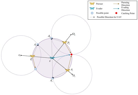
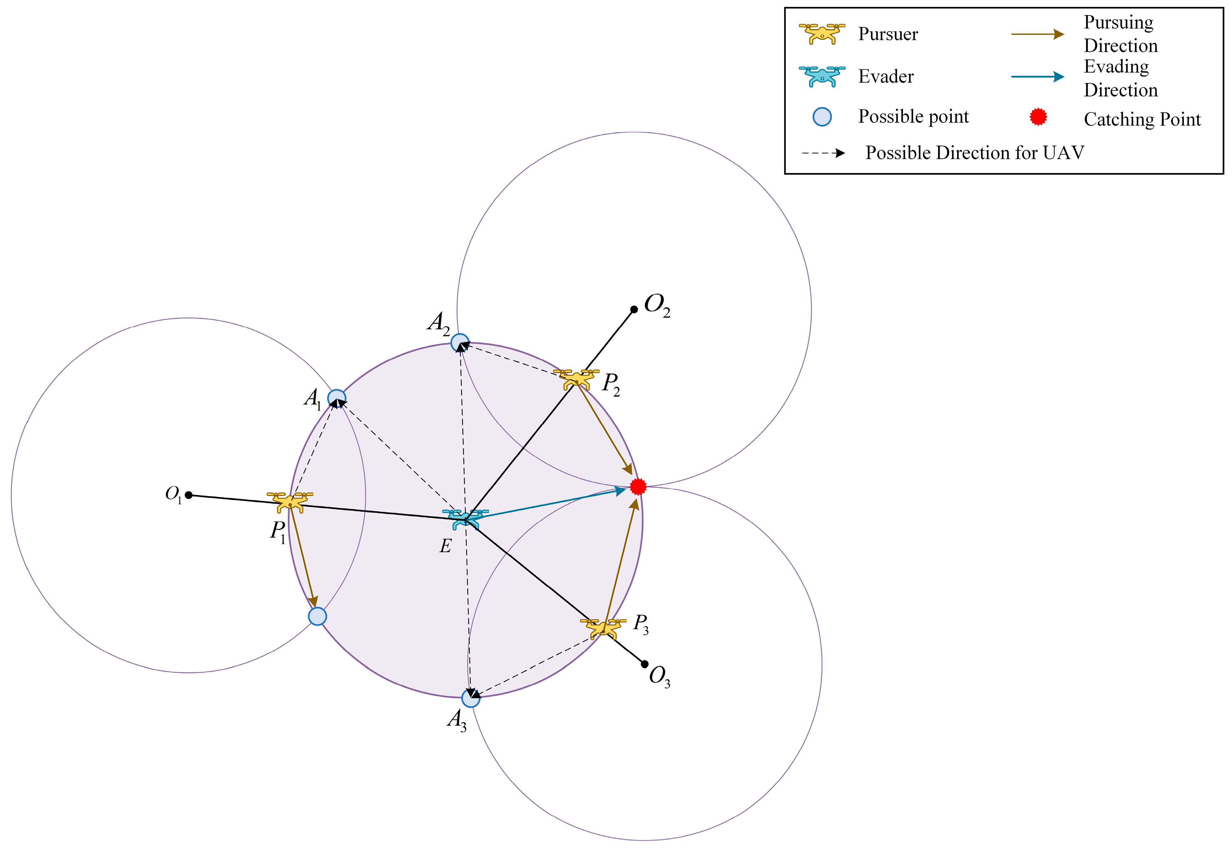
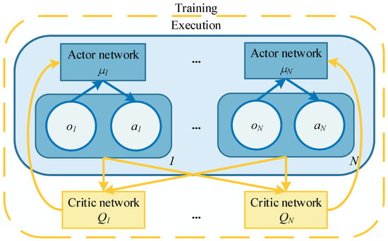
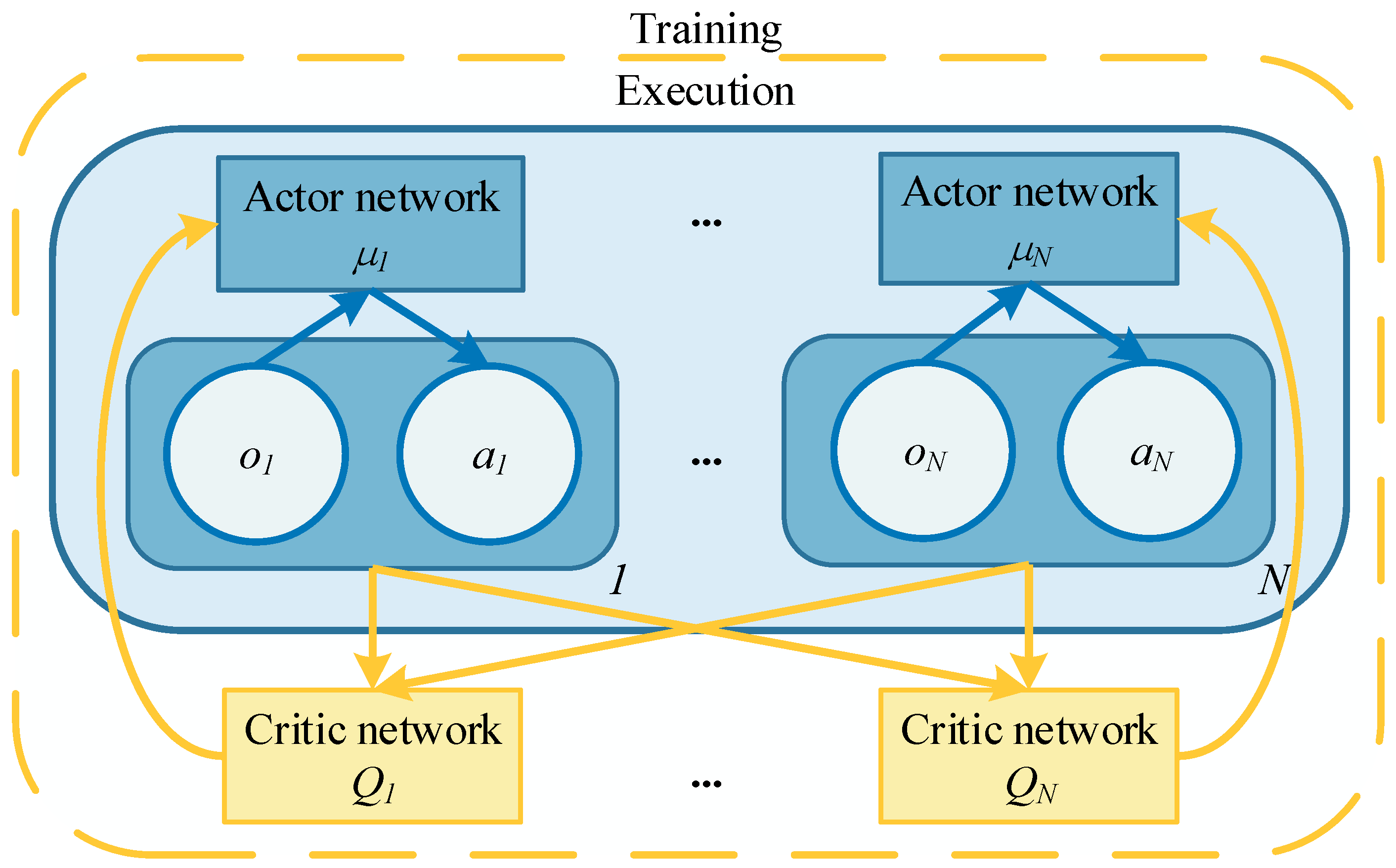
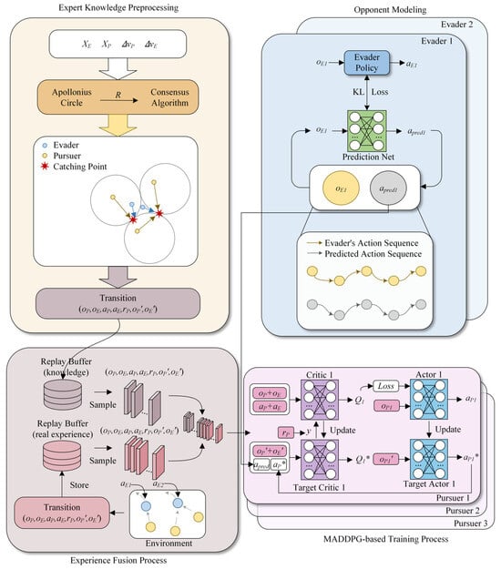
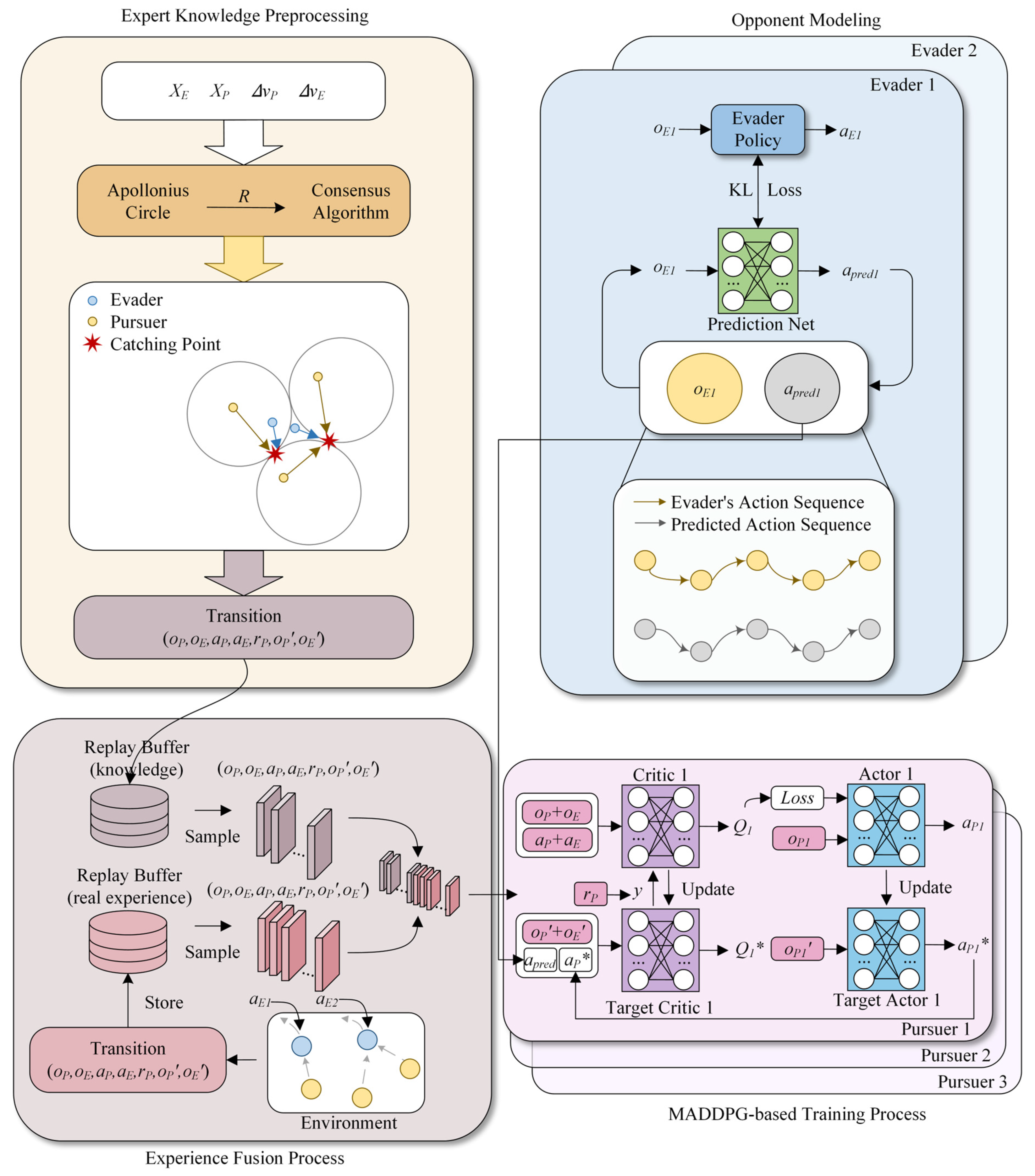
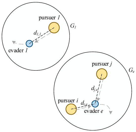
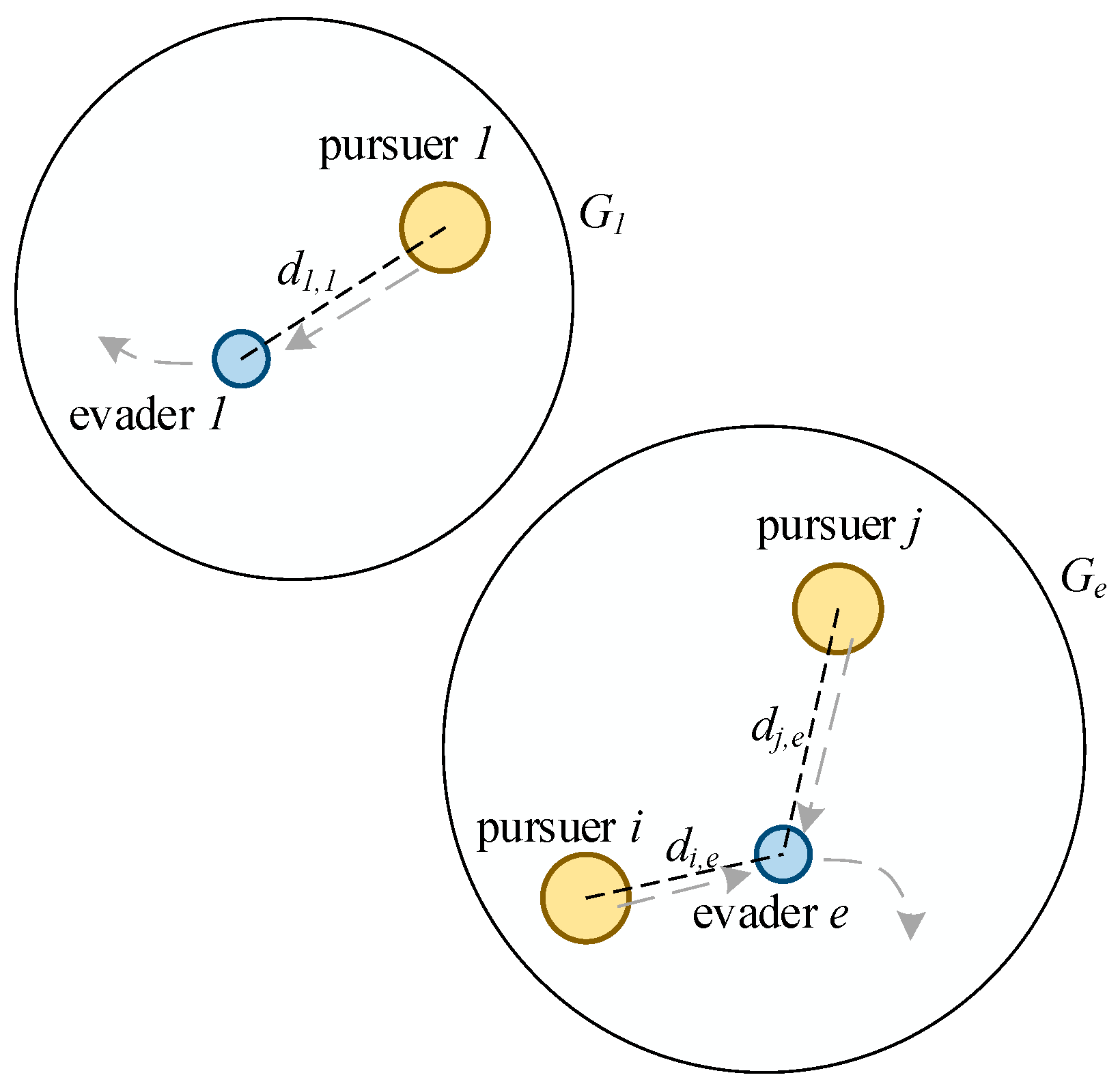
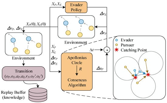
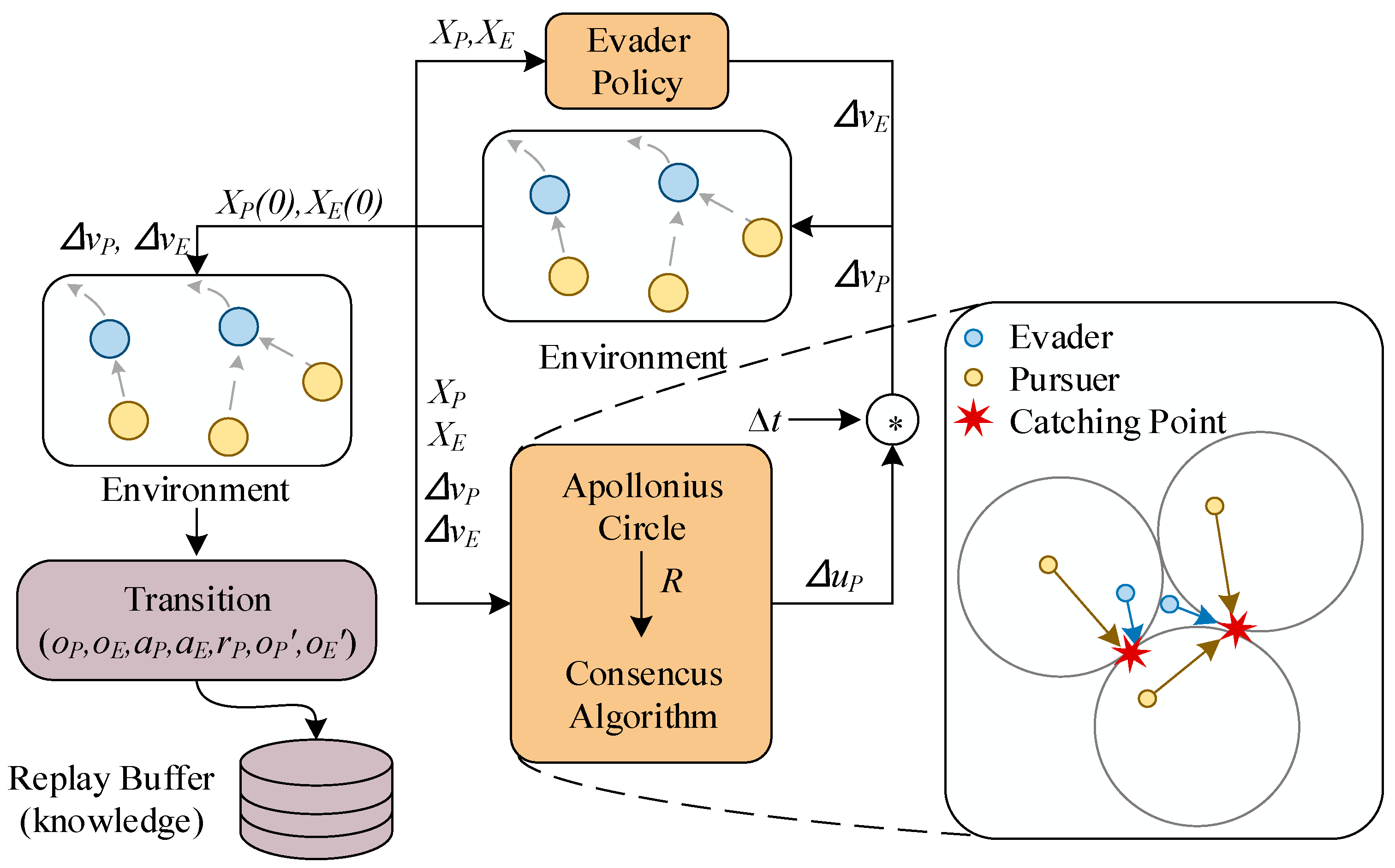
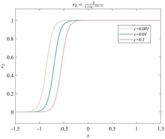
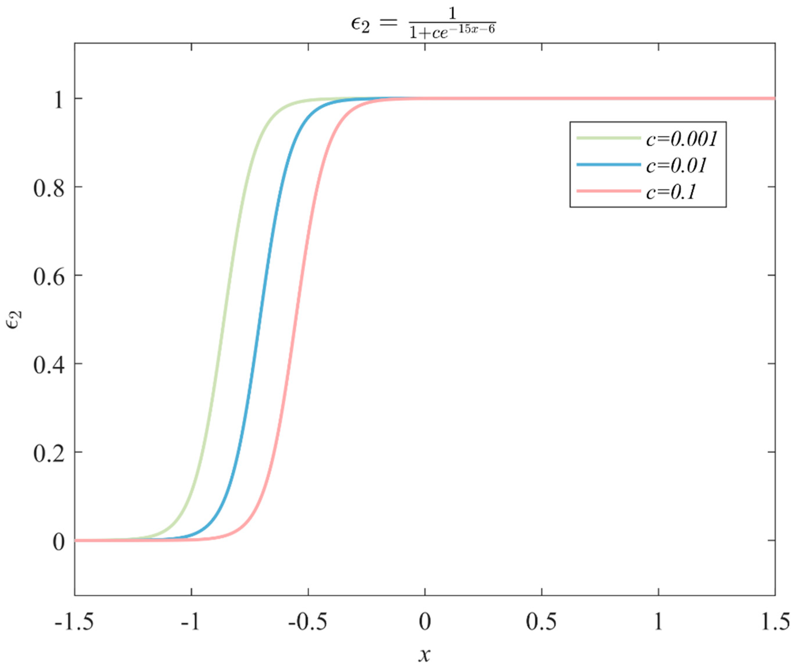
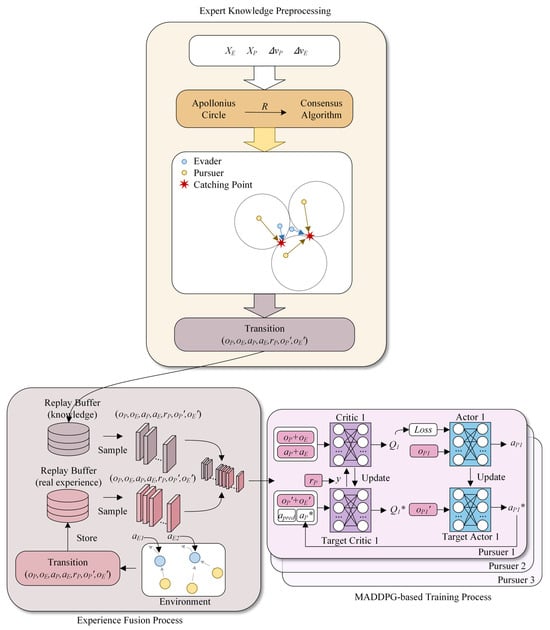
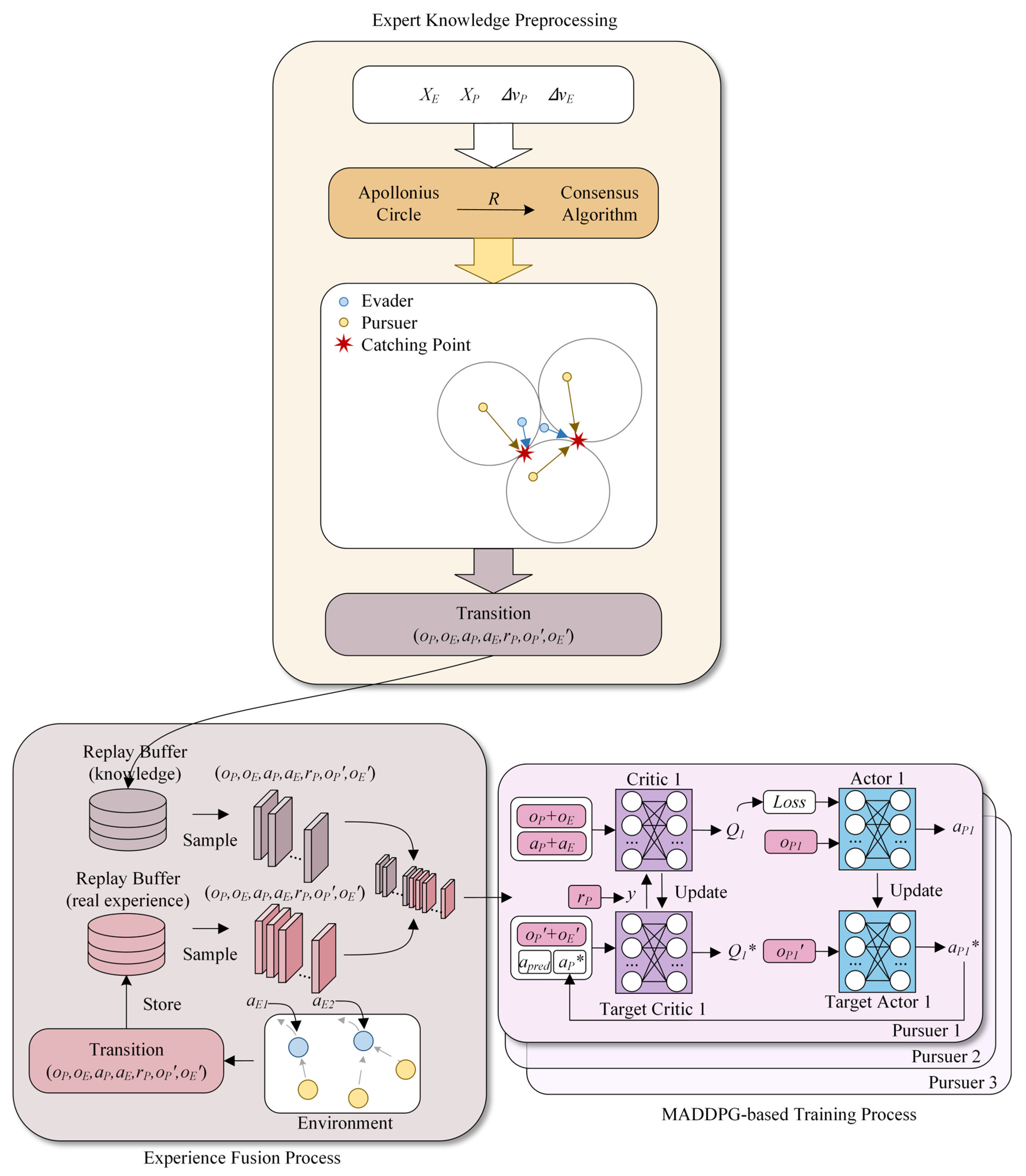
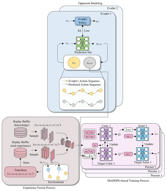
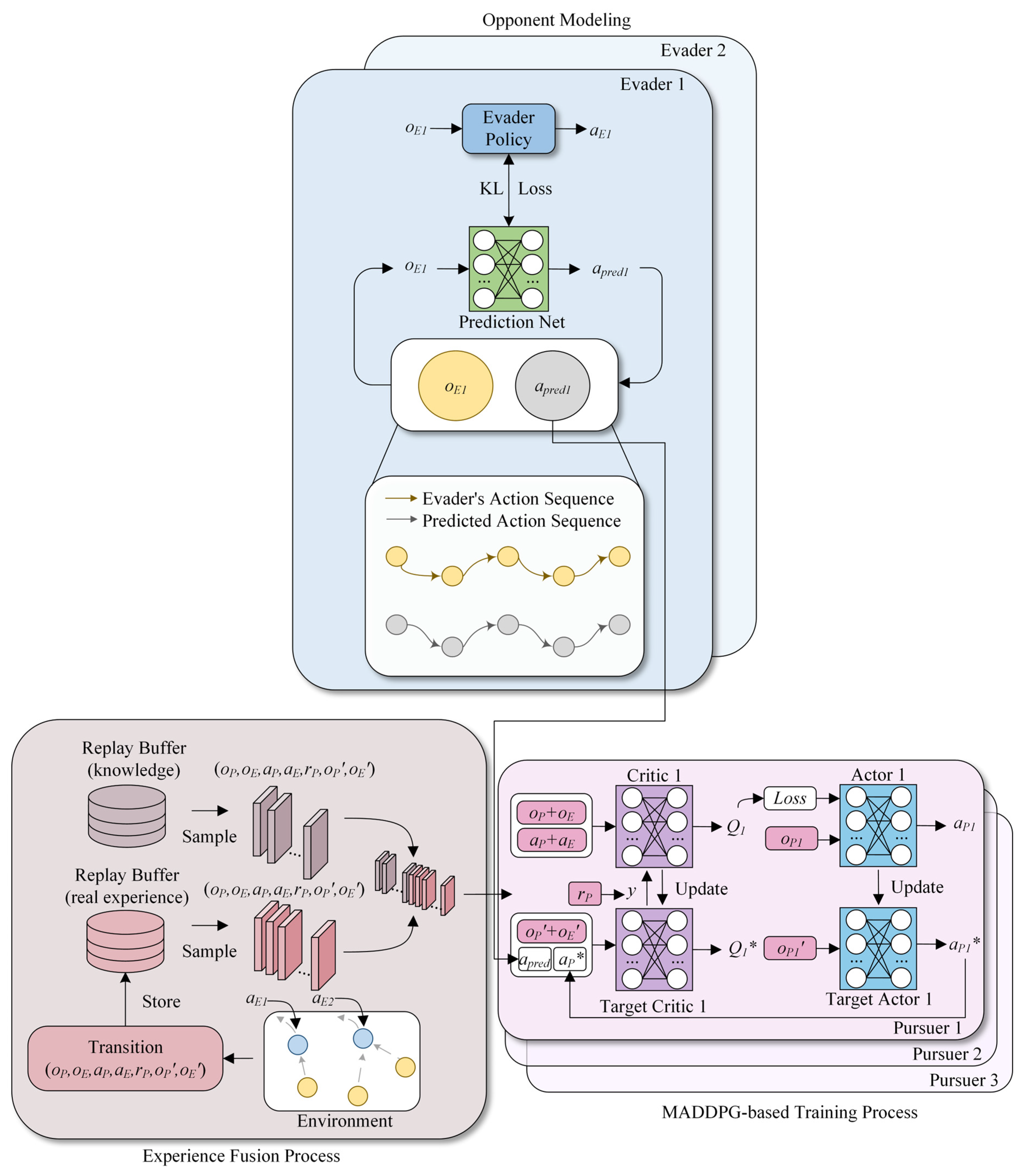
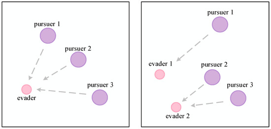
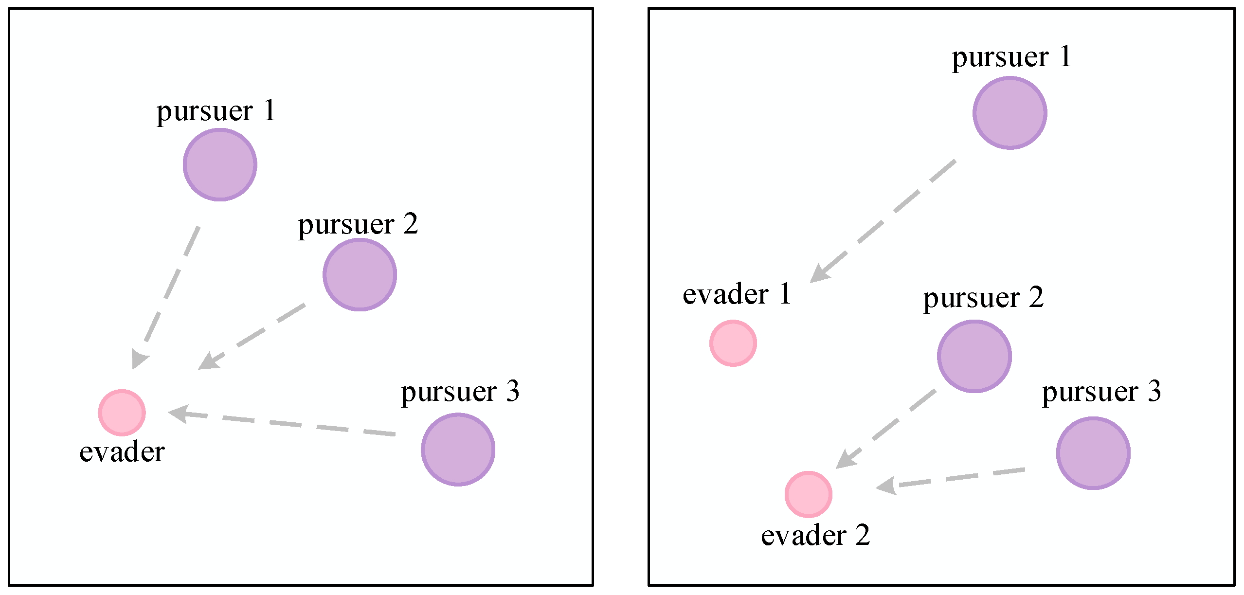
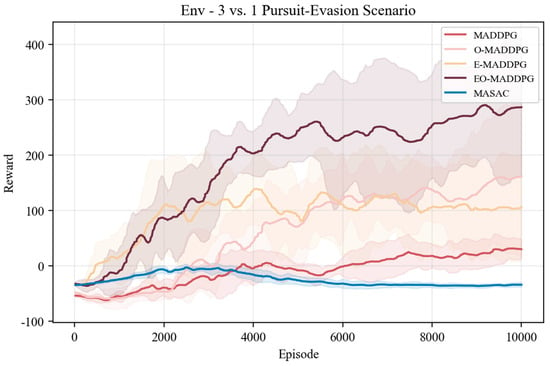
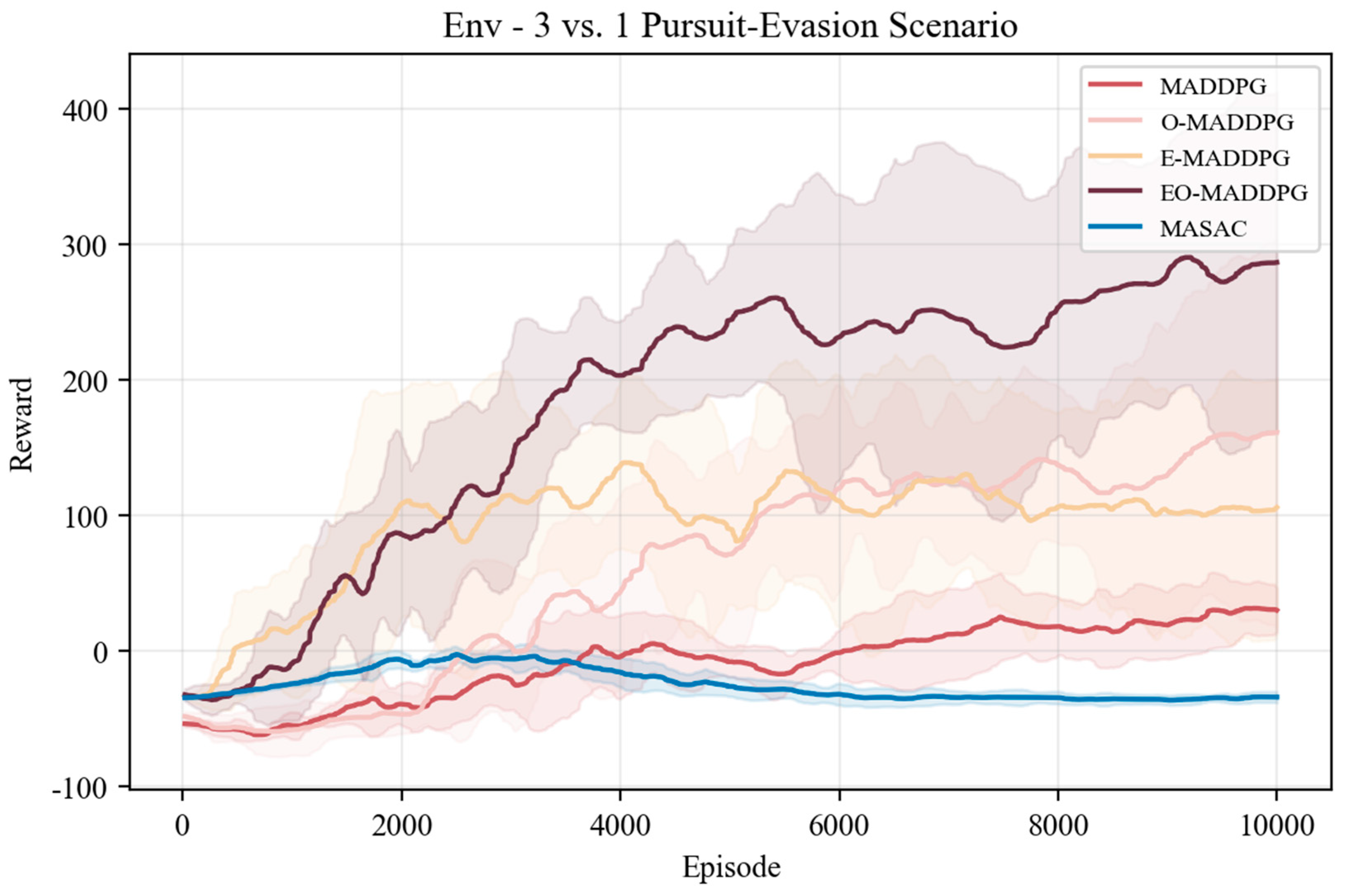
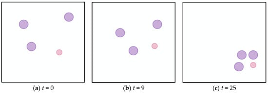
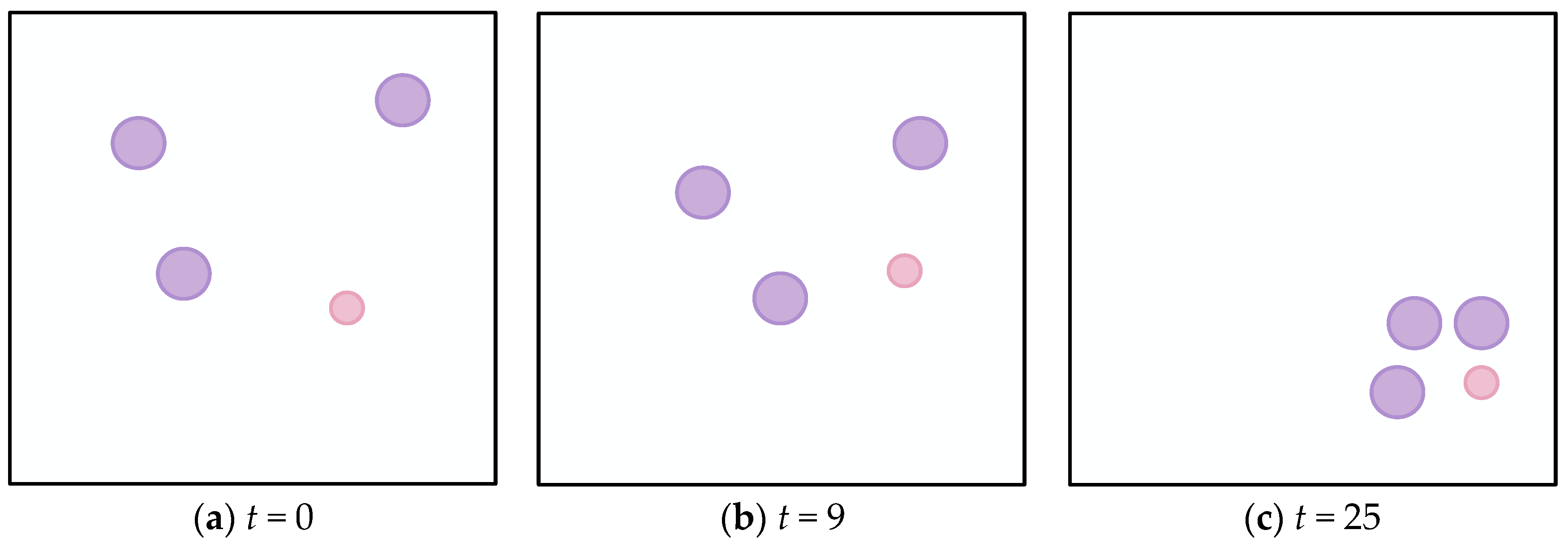
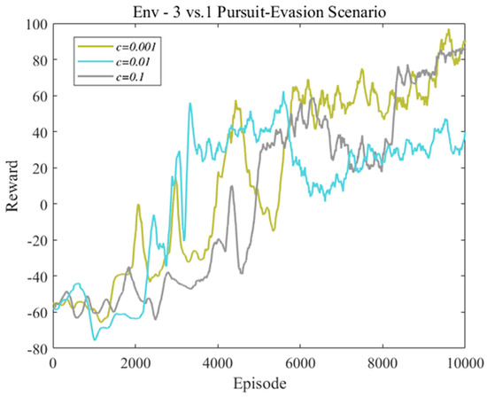
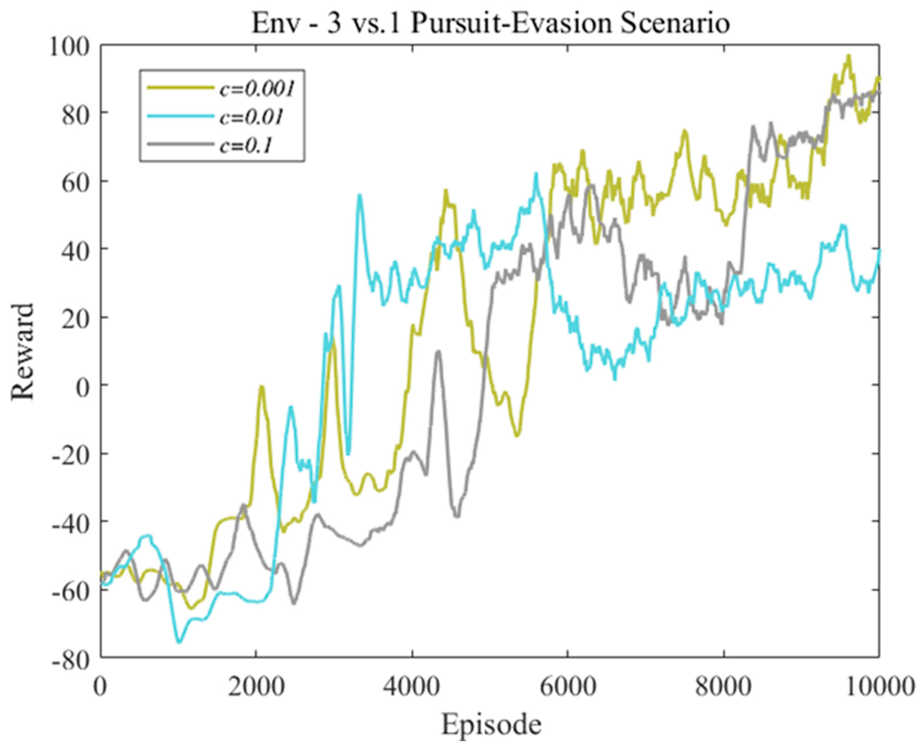
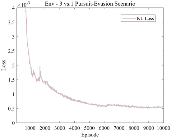
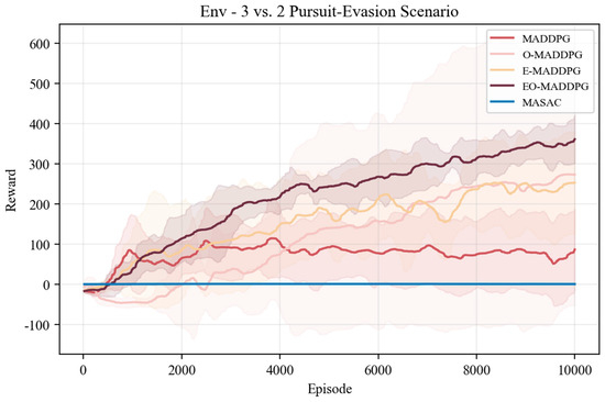
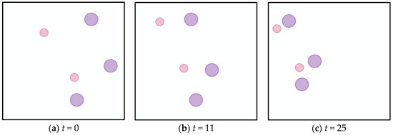
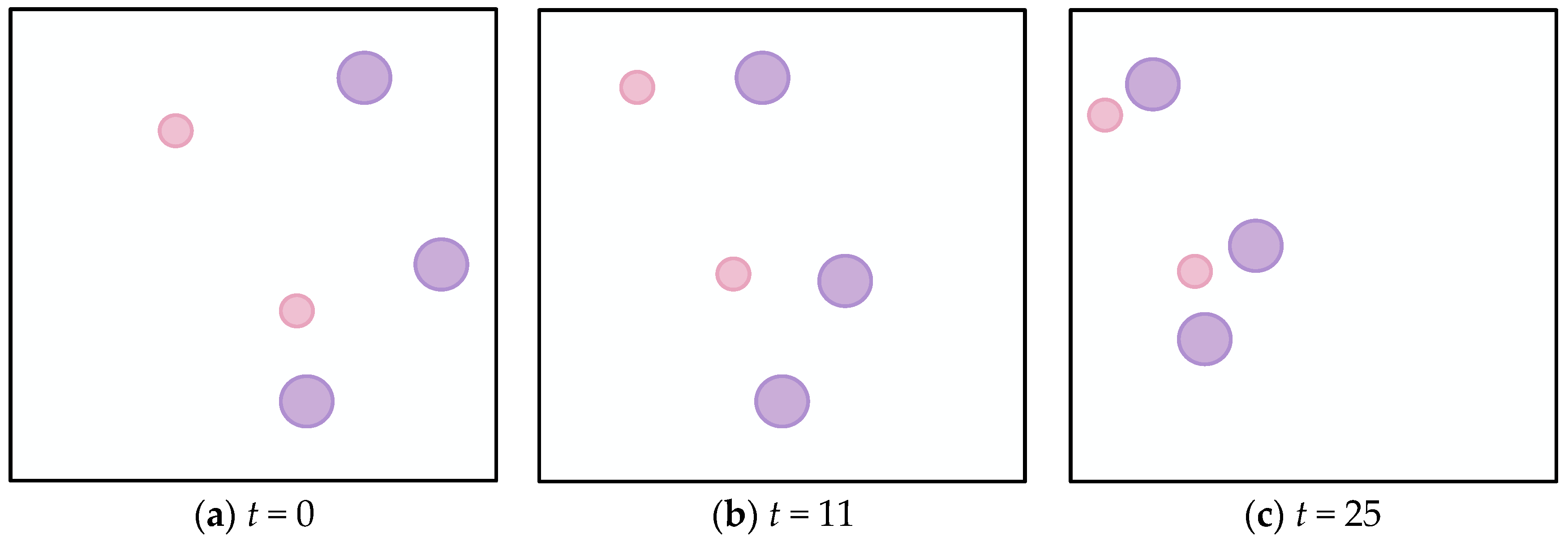
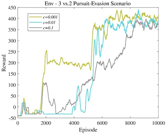
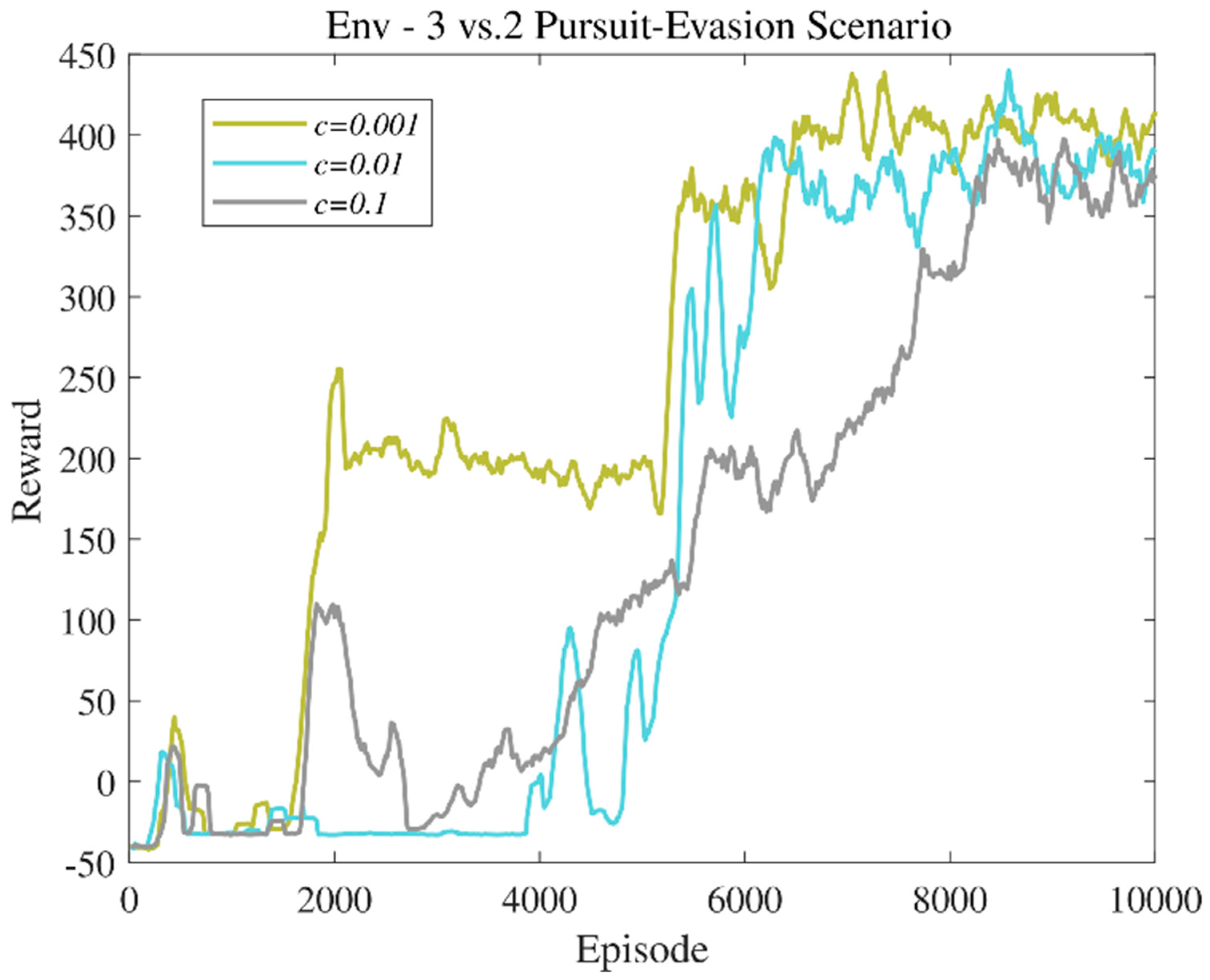
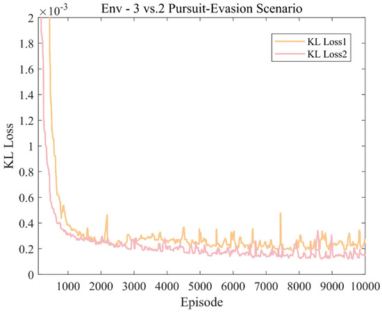
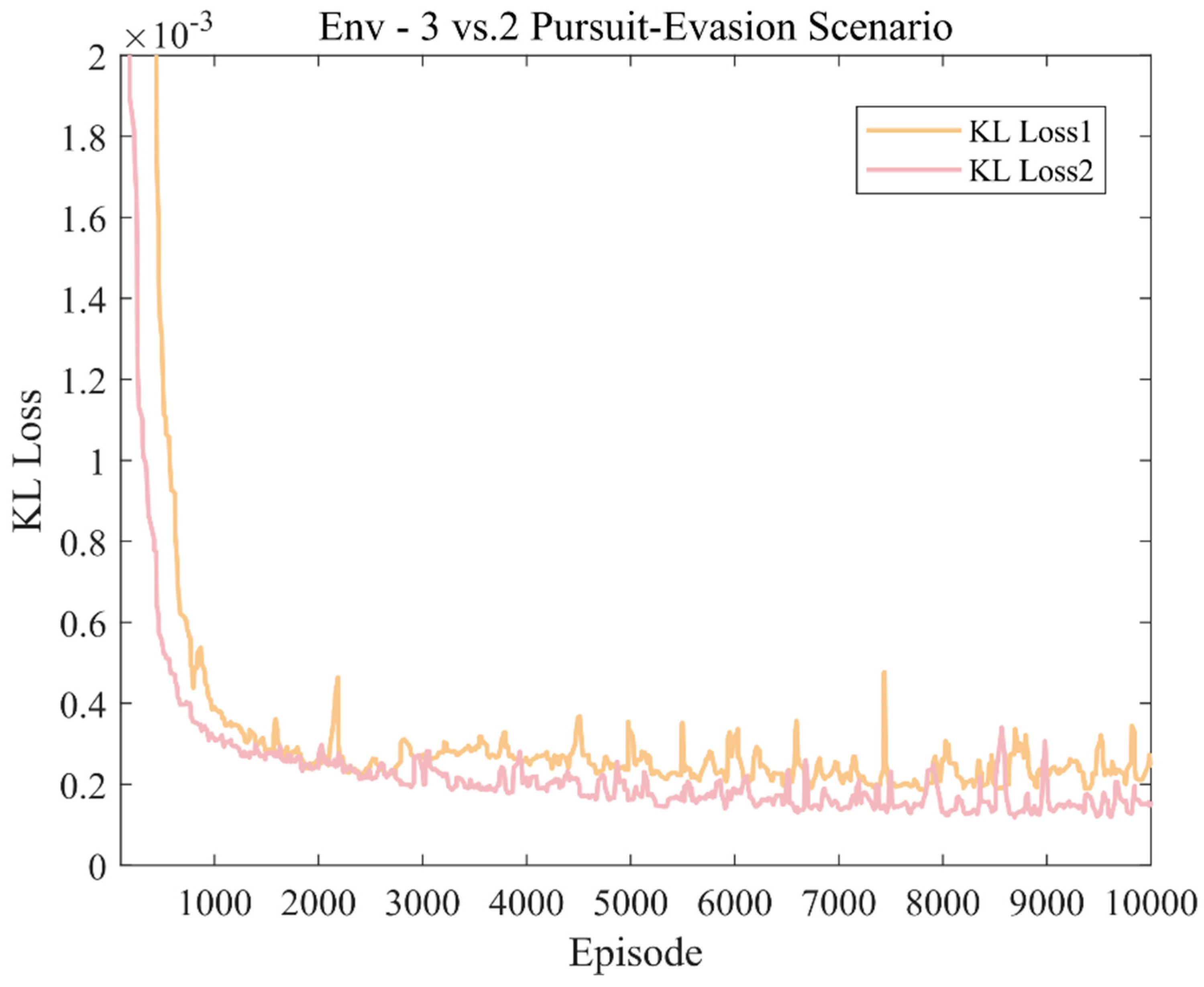
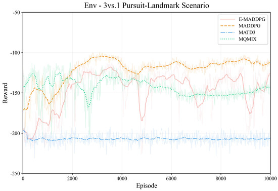
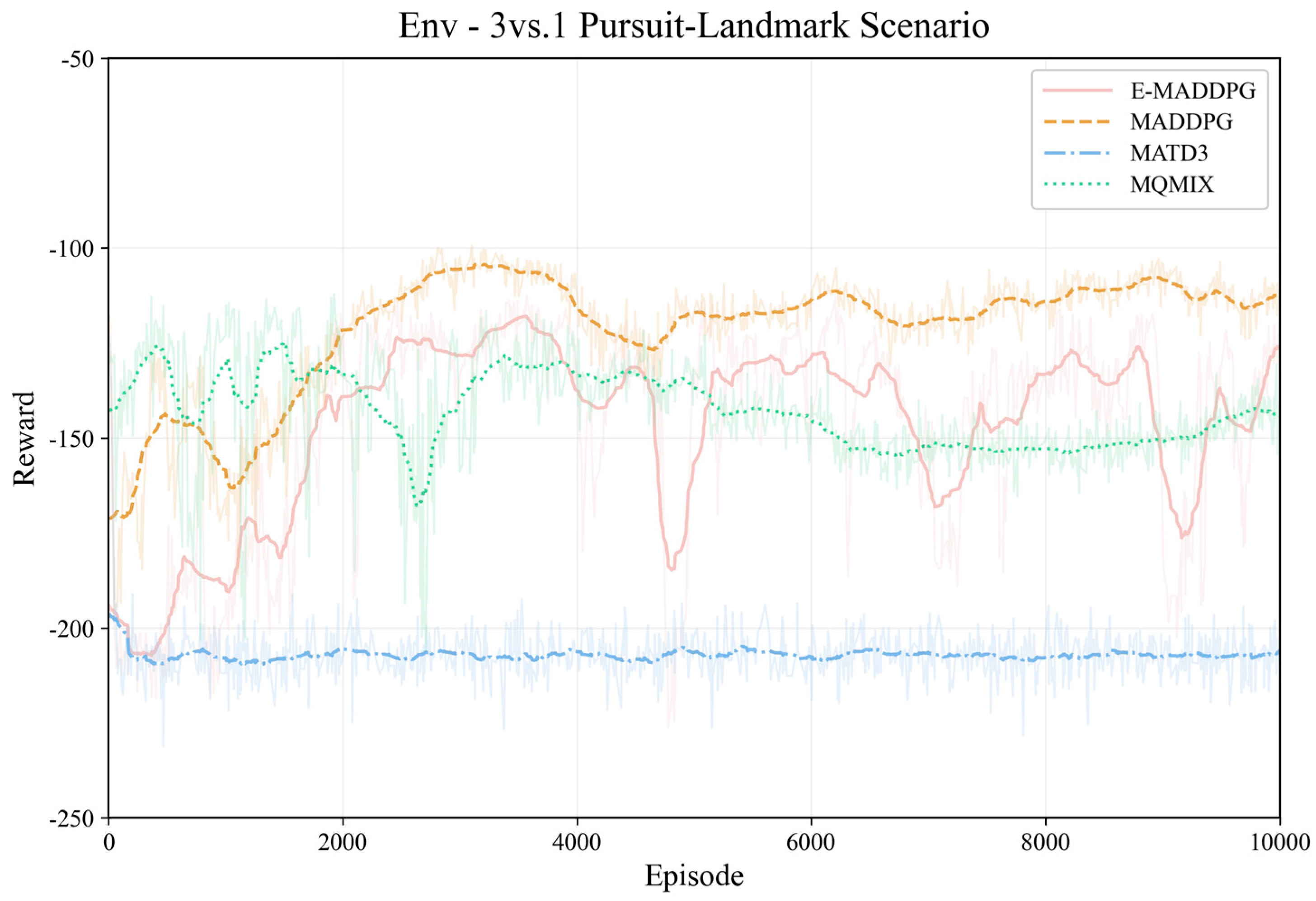
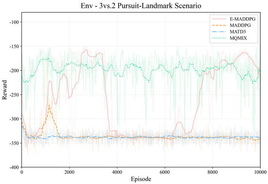
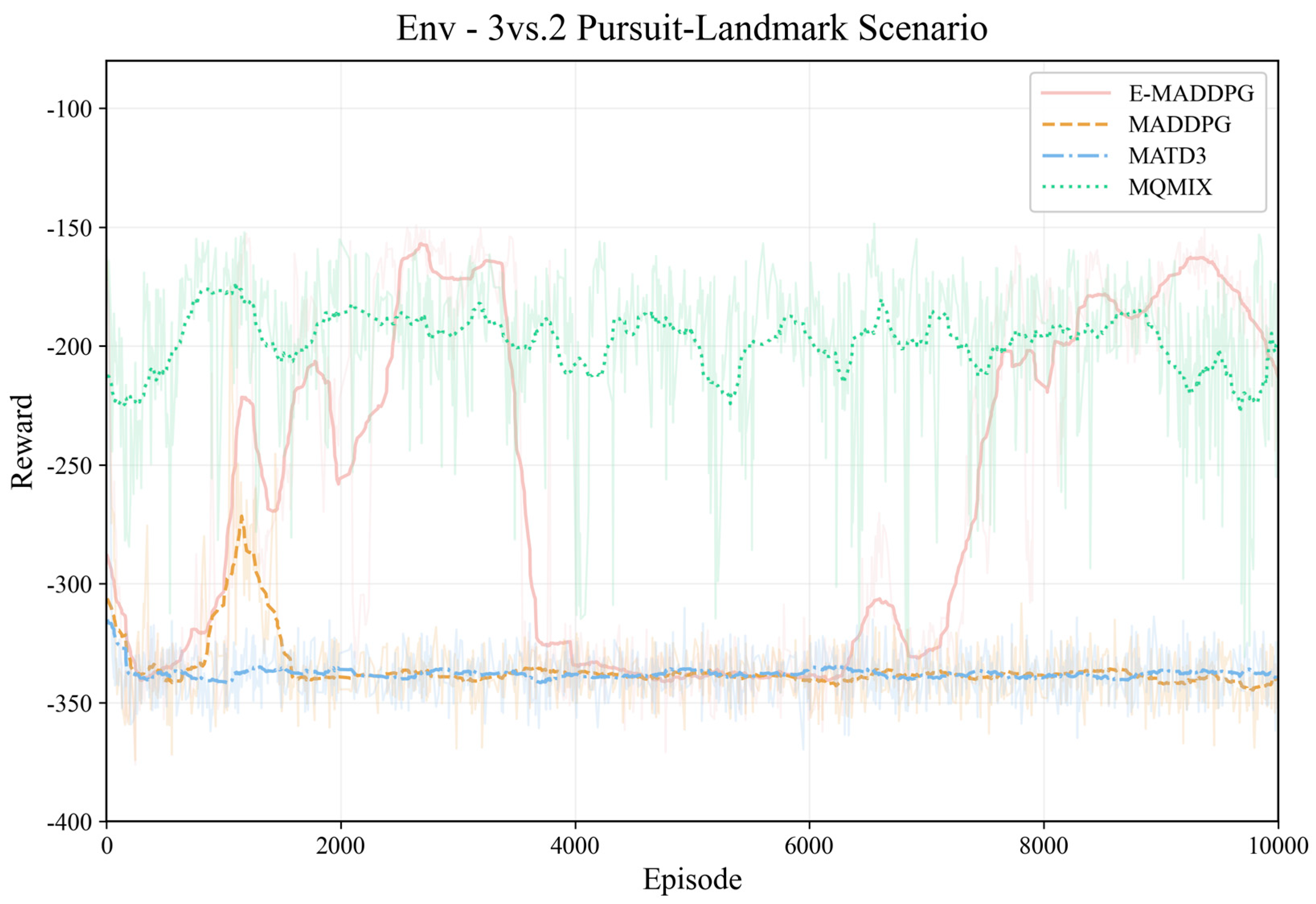

Disclaimer/Publisher’s Note: The statements, opinions and data contained in all publications are solely those of the individual author(s) and contributor(s) and not of MDPI and/or the editor(s). MDPI and/or the editor(s) disclaim responsibility for any injury to people or property resulting from any ideas, methods, instructions or products referred to in the content. |
© 2026 by the authors. Licensee MDPI, Basel, Switzerland. This article is an open access article distributed under the terms and conditions of the Creative Commons Attribution (CC BY) license.