Intelligent Propagation for an Inclined Geosynchronous Orbit Using Mean Elements

Abstract

High-accuracy propagation for an inclined geosynchronous orbit (IGSO) is of great importance to region navigation enhancement. Mean orbital elements enable accurate and efficient long-term propagation, particularly for large-scale computations. However, due to errors in transformations between mean and oscillating elements and mean dynamics, the actual orbit drifts from the propagated IGSO. In order to increase the orbit accuracy, an intelligent propagation method for the IGSO with respect to the mean elements is developed. Transformation models between the mean and oscillating elements of the IGSO under a precise dynamic model are derived. The orbital perturbations on the IGSO with respect to non-singular elements are decomposed into secular and periodic terms based on an averaged method. Mean dynamic errors degrading long-term propagation and errors in short-period terms affecting transformation are identified and separated. To neutralize the errors and improve the long-term propagating accuracy, a neural network-based propagation method for the IGSO is established. The transforming and propagating errors are fitted and predicted using two individual deep neural networks. Training methods for both networks are constructed. Numerical simulations validate the performance of the proposed NN-based transformation method and the intelligent propagation method for the IGSO.

1. Introduction

An inclined geosynchronous orbit (IGSO) is a type of geosynchronous orbit. It has an orbital period of one sidereal day and a non-negligible inclination, which makes it one of the most important orbital resources for satellite navigation [1,2]. The Indian Space Research Organisation (ISRO) launched four IGSO satellites as part of the Navigation with Indian Constellation (NavIC) [3]. The China National Space Administration (CNSA) deployed three IGSO satellites for the BeiDou Navigation Satellite System (BDS) [4]. In a practical mission, the IGSO is subject to multiple orbital perturbations. In this situation, accurate orbit propagation of the IGSO satellite is essential [5].

Previous studies concluded that the perturbations including Earth’s nonspherical gravity, luni-solar gravitations and solar radiation pressure drift the intersection point of the IGSO ground track to drift away from its desired region [2]. Li et al. and Tang et al. analyzed the long-term evolution characteristics of BDS-IGSO satellites based on a simplified dynamic model and orbital elements [6,7]. The effects of the perturbations are isolated as secular terms and periodic terms. The secular terms represent the mean motions, while the periodic terms describe the periodic behaviors with respect to the orbital elements. A direct approach to obtain the IGSO is propagating the instantaneous oscillating elements which incorporate the secular terms and the periodic terms. However, complicated orbital perturbations make long-term propagation computationally expensive [8,9,10]. In order to improve the propagation efficiency and guarantee the accuracy, researchers removed the periodic terms, filtered the elements and integrated the orbit with the secular terms [11,12].

The process of removing and reintroducing the periodic terms is defined as transformation between the oscillating and mean elements. Soop developed a transformation framework for the mean and oscillating elements of the geostationary (GEO) satellite [13]. Celletti et al. derived the analytical expansions for luni-solar third-body gravitation perturbations [14]. The short-term and secular evolutions of the near-Earth orbits have been studied. Shen et al. extended this approach to a precise ephemeris model and derived corresponding short-period oscillation amplitudes [12]. An accurate transformation method for the GEO was provided. Due to the difference in orbital inclination, the GEO-based transformation method introduces errors in IGSO. Tan et al. derived short-period terms of the BDS-IGSO using an averaging method and Delaunay variables [15]. A dynamic model including fourth-order zonal harmonic and the second-order tesseral harmonic terms of non-spherical gravitation of the Earth and luni-solar gravitation has been considered. However, the proposed method neglected the high-order coupled effects of periodic evolutions under multiple perturbations and the imperfect elliptical orbits of the Sun and the Moon, leaving room for further improvement.

After transforming the oscillating elements into the mean elements, the long-term propagation of the IGSO can be performed through numerical and semi-analytical integrations [8,16]. Kozai proposed an averaged method to remove the short-period terms of the perturbations [17]. Then, a general propagation method with respect to the mean elements was established. The key to accurate orbit propagation is adopting a high-fidelity mean dynamic model. Tang et al. and Gkolias et al. considered dynamic models including the J2 non-spherical gravitation of the Earth and luni-solar gravitations [7,18]. The Keplerian elements of the IGSO were calculated through numerical propagation. Tan et al. constructed a semi-analytical propagator for the IGSO based on a double-averaged method [15]. The Earth’s gravitation was extended to fourth-order zonal harmonic terms. The long-term propagation accuracy with respect to the mean elements is improved. Shen et al. developed a precise propagation method for the mean elements of the GEO [12]. A high-fidelity dynamic model covering fourth-order zonal and tesseral harmonic terms of the non-spherical gravitation of the Earth, luni-solar gravitations and solar radiation pressure was introduced. However, as highlighted above, the GEO-based propagation method is unavailable for the IGSO due to the high inclination. In addition, the dynamic models of these methods neglected the high-order truncation errors in derivation and the coupled effects of the mean motions, which limits the long-term propagation accuracy.

To deal with the transforming and propagating errors caused by coupled effects, truncations and ephemeris, studies on correction methods have been carried out [19]. Sasfi et al. employed a polyhedron-based model to fit and predict the dynamic errors [20]. However, the geometric characteristics of the dynamic errors of the IGSO appear strongly non-linear and time-varying. Analytical methods cannot guarantee the accuracy of error prediction. Machine learning methods show the ability to identify, fit and predict the non-linear errors [19]. Neural network-based (NN-based) methods have been widely employed in the research directions of navigation [21,22,23], attitude control [24,25,26] and orbital uncertainty estimation [27,28]. The dynamic errors were neutralized using trained networks to effectively improve the state accuracies of estimation and prediction. Moreover, Huang et al., Federici et al. and Fereoli et al. developed intelligent guidance methods based on reinforcement learning [19,29,30]. The dynamic uncertainties were fitted and predicted online to increase the guidance accuracy. Therefore, neutralizing the transforming and propagating errors via NNs to increase the propagation accuracy of the IGSO is feasible and necessary.

Since typical transforming and propagating methods for the GEO satellite are simplified considering a zero-degree condition of the inclination, these methods are inadequate for the IGSO. According to the dynamic model of geosynchronous orbit family, the motion of every orbital element is affected by the inclination. Regarding the IGSO, high-order coupled effects in the secular terms and periodic terms caused by a high inclination cannot be simplified. Moreover, these high-order coupled terms are difficult to derive analytically since they show strong nonlinearity and large scale. Therefore, in the present paper, a propagating method for the IGSO is developed. The high-order coupled effects in the secular and periodic terms are fitted and predicted via deep neural networks. The main contributions of this work are summarized as follows:

(1) Following previous work [12] which derived precise oscillating and mean models of the GEO, the present study extends these models to the IGSO with respect to non-singular elements. The perturbations of four orders of zonal harmonics and tesseral harmonics terms of the Earth’s non-spherical gravitation, luni-solar gravitations and solar radiation pressure are decomposed into secular and periodic terms based on an averaging method.

(2) Referring to [15] which established transformations between oscillating and mean elements of the GEO, in the present study, intelligent transforming models of the elements with respect to the IGSO are built upon. High-order coupled errors of the periodic-term perturbations are fitted and neutralized using a deep neural network to guarantee the matching accuracy.

(3) Inspired by [19] which compensated the uncertainties in dynamic parameters to increase the propagation accuracy, an intelligent propagation method for the IGSO with respect to the mean elements is developed. High-order coupled errors of the mean dynamics are fitted and predicted using a deep neural network to improve the long-term propagation accuracy.

The rest of this paper is organized as follows: In Section 1, the dynamics of the IGSO satellite are defined. Section 2 constructs the transformation model between the mean and oscillating elements. The secular terms and short-period terms are derived. The intelligent propagation method for the IGSO and the NN-based error prediction method are provided in Section 3. Section 4 validates the intelligent transformation method and the intelligent propagation method by numerical simulations. Finally, Section 5 presents the conclusions of this paper.

2. Dynamics of the IGSO Satellite

2.1. Non-Singular Orbital Elements

An IGSO satellite operates in an inclined, near-circular orbit in an Earth-centered inertial (ECI) coordinate system, with an orbital period equaling the rotation period of the Earth. In the ECI system, the X axis points to the equinox, the Z axis coincides with the Earth’s rotation axis, while the Y axis completes an orthogonal system. Meanwhile, owing to the near-circular condition, the high-order terms of the eccentricity are approximately zero, e² ≈ 0. To avoid singularities, non-singular orbital elements are employed to describe the IGSO satellite as follows:

[a,e_x,e_y,i_x,i_y,L]

(1)

where a, L denote the semi-major axis and mean longitude, respectively. The symbols (e_x, e_y) represent the eccentricity vectors; (i_x, i_y) represent the inclination vectors, which are denoted as follows:

$$\left\{\begin{array}{c}{e}_{\mathrm{x}}=e\cos \left(\mathrm{\Omega }+\omega \right)\hfill \\ e_{\mathrm{y}}=e\sin \left(\mathrm{\Omega }+\omega \right)\end{array}\right.$$

(2)

$$\left\{\begin{array}{c}{i}_{\mathrm{x}}=\sin i\cos \mathrm{\Omega }\hfill \\ i_{\mathrm{y}}=\sin i\sin \mathrm{\Omega }\end{array}\right.$$

(3)

λ = Ω + ω + M

(4)

L = λ − θ(t)

(5)

where e, i, Ω, ω, M denote the eccentricity, the inclination, the right ascension of ascending node, the argument of perigee and the mean anomaly, respectively.

2.2. Dynamic Model

According to previous studies [12], the IGSO satellite suffers from dynamic perturbations including Earth’s non-spherical gravitation, luni-solar third-body gravitations and solar radiation pressure. The perturbing potential R of the IGSO satellite is given as follows:

R = R_E + R_T + R_S

(6)

where the subscripts E, T, S denote the perturbations of Earth’s non-spherical gravitation, luni-solar third-body gravitations and solar radiation pressure, respectively.

The perturbing potential of the Earth’s non-spherical gravitation up to four orders of zonal harmonics and tesseral harmonics terms is given by

$$\begin{array}{cc}\hfill R_{\mathrm{E}}& ={\displaystyle \frac{{\mu }_{\mathrm{E}}}{r}}\left[{\displaystyle \frac{J_{2,0}{r}_{\mathrm{E}}^2}{2r^2}}\left(3{\sin }^2\phi -1\right)+{\displaystyle \frac{3J_{22}{r}_{\mathrm{E}}^2}{r^2}}{\cos }^2\phi \cos \left[2\left(L-L_{22}\right)\right]\right.\hfill \\ & +{\displaystyle \frac{3J_{31}{r}_{\mathrm{E}}^3}{2r^3}}\cos \phi \left(5{\sin }^2\phi -1\right)\cos \left(L-L_{31}\right)+{\displaystyle \frac{15J_{33}{r}_{\mathrm{E}}^3}{r^3}}{\cos }^3\phi \cos \left[3\left(L-L_{33}\right)\right]\hfill \\ & +{\displaystyle \frac{J_{4,0}{r}_{\mathrm{E}}^4}{8r^4}}\left(35{\sin }^4\phi -30{\sin }^2\phi +3\right)+{\displaystyle \frac{15J_{42}{r}_{\mathrm{E}}^4}{2r^4}}{\cos }^2\phi \left(7{\sin }^2\phi -1\right)\cos \left[2\left(L-L_{42}\right)\right]\hfill \\ & \left.+{\displaystyle \frac{105J_{44}{r}_{\mathrm{E}}^4}{r^4}}{\cos }^4\phi \cos \left[4\left(L-L_{44}\right)\right]\right]\hfill \end{array}$$

(7)

where μ_E denotes the gravity parameter of the Earth, μ_E = 398,600 km³/s²; r represents the geocentric distance of the IGSO satellite; r_E represents the radius of the Earth, r_E = 6378.137 km; J_m,n and L_m,n are [m, n] orders of harmonics coefficient and specific longitude of the Earth’s non-spherical gravitation, respectively; φ represents the latitude of the IGSO satellite.

The perturbing potential of the luni-solar gravitations is given by

$$R_{\mathrm{T}}={\mu }_{\mathrm{T}}\left({\displaystyle \frac{1}{‖{\mathit{r}}_{\mathrm{T}}-\mathit{r}‖}}-{\displaystyle \frac{r}{r_{\mathrm{T}}^2}}\cos {\theta }_{\mathrm{T}}\right)$$

(8)

where r denotes the position vector of the IGSO satellite; r_T denotes the position vectors, i.e., the ephemerides, of the Sun and the Moon in the ECI system, r_T = [x_T;y_T;z_T]; θ_T is the angle between r and r_T, ${\theta }_{\mathrm{T}}={\displaystyle \frac{x_{\mathrm{T}}\sin \lambda \cos \phi +y_{\mathrm{T}}\cos \lambda \cos \phi +z_{\mathrm{T}}\sin \phi }{r_{\mathrm{T}}}}$.

The perturbing potential of the solar radiation pressure is given by

$$R_{\mathrm{S}}=-C_{\mathrm{R}}{\displaystyle \frac{A}{m}}{P}_0\left(x_{\mathrm{S}}x+y_{\mathrm{S}}y+z_{\mathrm{S}}z\right)$$

(9)

where C_R denotes the radiation pressure coefficient; A and m represent the area and mass of the IGSO satellite; P₀ denotes the solar radiation pressure constant, P₀ = 4.65 × 10⁻⁶ N/m².

3. Transformation of IGSO

3.1. Transformation Between the Mean and Oscillating Elements

In order to construct a transformation model between the mean and oscillating elements, the dynamic model of the IGSO satellite with respect to the non-singular elements is derived. Current studies indicate that the instantaneous motions of the IGSO can be decomposed into secular terms and short-period terms. The instantaneous motions, i.e., the oscillating elements, denote the real-time states of the IGSO; the secular terms, defining the mean motions, suggest the long-term evolution behavior; the short-period terms are related to the motion of the IGSO satellite around the Earth. The dynamic model of the IGSO with respect to the non-singular elements is given by

$$\dot{\zeta }=\overline{\dot{\zeta }}+{\dot{\zeta }}_{\mathrm{SP}}$$

(10)

where ζ represents the non-singular elements; the subscript SP denotes the short-period terms.

The rates of change of the non-singular elements with respect to the perturbing potential are derived based on the Lagrange planetary equations as follows:

$$\left\{\begin{array}{l}\dot{a}={\displaystyle \frac{2}{\mathit{na}}}{\displaystyle \frac{\partial R}{\partial L}}\\ {\dot{e}}_x=-{\displaystyle \frac{1}{n{a}^2}}{\displaystyle \frac{\partial R}{\partial e_y}}\\ {\dot{e}}_y={\displaystyle \frac{1}{n{a}^2}}{\displaystyle \frac{\partial R}{\partial e_x}}\\ {\dot{i}}_x=-{\displaystyle \frac{1}{n{a}^2}}{\displaystyle \frac{\partial R}{\partial i_y}}\\ {\dot{i}}_y={\displaystyle \frac{1}{n{a}^2}}{\displaystyle \frac{\partial R}{\partial i_x}}\\ \dot{L}=-{\displaystyle \frac{2}{\mathit{na}}}{\displaystyle \frac{\partial R}{\partial a}}\end{array}\right.$$

(11)

Then, the mean rates of change of the non-singular elements are obtained using an averaging method as follows:

$$\overline{\dot{\zeta }}={\displaystyle {\int }_0^T\dot{\zeta }\mathrm{d}t}$$

(12)

where T represents the orbital period of the IGSO.

The transformation from the oscillating elements ζ to the mean elements $\overline{\zeta }$ is conducted by eliminating the short-period terms Δζ_SP, which is given in Equation (13). The short-period terms Δζ_SP are obtained through indefinite integration.

$$\left\{\begin{array}{l}\zeta =\overline{\zeta }+\Delta {\zeta }_{\mathrm{SP}}\\ \Delta {\zeta }_{\mathrm{SP}}={\displaystyle \int {\dot{\zeta }}_{\mathrm{SP}}\mathrm{d}t}\end{array}\right.$$

(13)

3.2. Terms of Semi-Major Axis

Based on Equations (7), (11) and (12), the mean rate of change of the semi-major axis is given in Equation (14). Derivation results show that the averaged effects of the luni-solar gravitations and solar radiation pressure are 0. In this situation, the mean rate of change of the semi-major axis is determined by the non-spherical gravitation of the Earth. Equation (14) can be simplified as $\overline{\dot{a}}={\overline{\dot{a}}}_{\mathrm{E}}$. In order to simplify the derivation, a first-order Taylor expansion is executed with respect to sinφ, the term ${\displaystyle \frac{\partial \left(\cos {\theta }_{\mathrm{T}}\right)}{\partial L}}={\displaystyle \frac{-x_{\mathrm{T}}\sin \lambda \cos \phi +y_{\mathrm{T}}\cos \lambda \cos \phi }{r_{\mathrm{T}}}}$.

$$\overline{\dot{a}}={\overline{\dot{a}}}_{\mathrm{E}}+{\overline{\dot{a}}}_{\mathrm{T}}+{\overline{\dot{a}}}_{\mathrm{S}}$$

(14)

$$\begin{array}{cc}\hfill {\overline{\dot{a}}}_{\mathrm{E}}& ={\displaystyle \frac{2\sqrt{{\mu }_{\mathrm{E}}}}{\sqrt{a}}}\left[{\displaystyle \frac{6J_{22}{r}_{\mathrm{E}}^2}{2a^2}}\left(-2+{\sin }^{2}i\right)\sin \left[2\left(L-L_{22}\right)\right]+{\displaystyle \frac{3J_{31}{r}_{\mathrm{E}}^3}{\pi a^3}}E\left(\sin i\right)\sin \left(L-L_{31}\right)\right.\hfill \\ & -{\displaystyle \frac{30J_{33}{r}_{\mathrm{E}}^3}{\pi a^3}}\left[\left(4-2{\sin }^{2}i\right)E\left(\sin i\right)-\left(1-{\sin }^{2}i\right)K\left(\sin i\right)\right]\sin \left[3\left(L-L_{33}\right)\right]\hfill \\ & +{\displaystyle \frac{15J_{42}{r}_{\mathrm{E}}^4}{8a^4}}\left(8-32{\sin }^{2}i+21{\sin }^{4}i\right)\sin \left[2\left(L-L_{42}\right)\right]\hfill \\ & \left.-{\displaystyle \frac{105J_{44}{r}_{\mathrm{E}}^4}{2a^4}}\left(8-8{\sin }^{2}i+3{\sin }^{4}i\right)\sin \left[4\left(L-L_{44}\right)\right]\right]\hfill \end{array}$$

(15)

$$\left\{\begin{array}{l}E\left(\sin i\right)={\displaystyle {\int }_0^{\frac{\pi }{2}}\sqrt{1-{\sin }^{2}i{\sin }^2\varphi }\mathrm{d}\varphi }\\ K\left(\sin i\right)={\displaystyle {\int }_0^{\frac{\pi }{2}}\frac{1}{\sqrt{1-{\sin }^{2}i{\sin }^2\varphi }}\mathrm{d}\varphi }\end{array}\right.$$

(16)

The periodic terms of the semi-major axis are given in Equation (17). For the IGSO, the oscillation amplitude of the periodic term with respect to the non-spherical gravitation of the Earth is about ${\displaystyle \frac{\max \Delta a_{\mathrm{E},\mathrm{SP}}}{a}}\le {10}^{-7}$, which is one order of magnitude smaller than that of the luni-solar gravitations and solar radiation pressure. Therefore, the periodic terms of the semi-major axis are assumed as Δa_SP = Δa_T,SP + Δa_S,SP. Note that the periodic term of the non-spherical gravitation of the Earth is not neglected during the transformation; instead, it is fitted and neutralized using a neural network. Details are provided in the following sections.

Δa_SP = Δa_E,SP + Δa_T,SP + Δa_S,SP

(17)

$$\begin{array}{cc}\hfill \Delta a_{\mathrm{T},\mathrm{SP}}& =-2\sqrt{{\displaystyle \frac{a^3}{{\mu }_{\mathrm{E}}}}}{\displaystyle \frac{{\mu }_{\mathrm{T}}}{\left(n-n_{\mathrm{T}}\right)r_{\mathrm{T}}^2}}\left[-{\displaystyle \frac{3}{2}}{\displaystyle \frac{a}{r_{\mathrm{T}}}}\left({\cos }^2{\theta }_{\mathrm{T}}-{\displaystyle \frac{x_{\mathrm{T}}^2+y_{\mathrm{T}}^2+z_{\mathrm{T}}^2}{2}}\right)\right.\hfill \\ & +{\displaystyle \frac{a^2}{2r_{\mathrm{T}}^2}}\left(3\cos {\theta }_{\mathrm{T}}-5{\cos }^3{\theta }_{\mathrm{T}}\right)\hfill \\ & \left.+{\displaystyle \frac{5a^3}{8r_{\mathrm{T}}^2}}\left[6\left({\cos }^2{\theta }_{\mathrm{T}}-{\displaystyle \frac{x_{\mathrm{T}}^2+y_{\mathrm{T}}^2+z_{\mathrm{T}}^2}{2}}\right)-7\left({\cos }^4{\theta }_{\mathrm{T}}-{\displaystyle \frac{3{\left(x_{\mathrm{T}}^2+y_{\mathrm{T}}^2+z_{\mathrm{T}}^2\right)}^2}{8}}\right)\right]\right]\hfill \end{array}$$

(18)

$$\Delta a_{\mathrm{S},\mathrm{SP}}=-2\sqrt{{\displaystyle \frac{a^3}{{\mu }_{\mathrm{E}}}}}{C}_{\mathrm{R}}{\displaystyle \frac{A}{m}}{\displaystyle \frac{P_0}{n_{\mathrm{E}}}}\left(x_{\mathrm{T}}\cos \phi \cos \lambda +y_{\mathrm{T}}\cos \phi \sin \lambda +z_{\mathrm{T}}\sin \phi \right)$$

(19)

3.3. Terms of Mean Longitude

Similar to the semi-major axis, the mean rate of change of the mean longitude is given in Equation (20). The averaged effect of the solar radiation pressure on the mean longitude is 0, which makes the mean rate of change of the mean longitude become $\overline{\dot{L}}={\overline{\dot{L}}}_{\mathrm{E}}+{\overline{\dot{L}}}_{\mathrm{T}}$.

$$\overline{\dot{L}}={\overline{\dot{L}}}_{\mathrm{E}}+{\overline{\dot{L}}}_{\mathrm{T}}+{\overline{\dot{L}}}_{\mathrm{S}}$$

(20)

$$\begin{array}{cc}\hfill {\overline{\dot{L}}}_{\mathrm{E}}& =\left(n-{\omega }_{\mathrm{E}}\right)+{\displaystyle \frac{2\sqrt{{\mu }_{\mathrm{E}}}}{\sqrt{a}}}\left[{\displaystyle \frac{3J_{2,0}{r}_{\mathrm{E}}^2}{4a^4}}\left(-2+3{\sin }^{2}i\right)+{\displaystyle \frac{9J_{22}{r}_{\mathrm{E}}^2}{2a^4}}\left(2-{\sin }^{2}i\right)\cos \left[2\left(L-L_{22}\right)\right]\right.\hfill \\ & +{\displaystyle \frac{4J_{31}{r}_{\mathrm{E}}^3}{\pi a^5}}\left[\left(-8+10{\sin }^{2}i\right)E\left(\sin i\right)+5\left(1-{\sin }^{2}i\right)K\left(\sin i\right)\right]\cos \left(L-L_{31}\right)\hfill \\ & +{\displaystyle \frac{40J_{33}{r}_{\mathrm{E}}^3}{\pi a^5}}\left[\left(4-2{\sin }^{2}i\right)E\left(\sin i\right)-\left(1-{\sin }^{2}i\right)K\left(\sin i\right)\right]\cos \left[3\left(L-L_{33}\right)\right]\hfill \\ & +{\displaystyle \frac{5J_{4,0}{r}_{\mathrm{E}}^4}{64a^6}}\left(24-120{\sin }_{2}i+105{\sin }^{4}i\right)+{\displaystyle \frac{75J_{42}{r}_{\mathrm{E}}^4}{16a^6}}\left(-8+32{\sin }^{2}i-21{\sin }^{4}i\right)\cos \left[2\left(L-L_{42}\right)\right]\hfill \\ & \left.+{\displaystyle \frac{525J_{44}{r}_{\mathrm{E}}^4}{8a^6}}\left(8-8{\sin }^{2}i+3{\sin }^{4}i\right)\cos \left[4\left(L-L_{44}\right)\right]\right]\hfill \end{array}$$

(21)

$$\begin{array}{cc}\hfill {\overline{\dot{L}}}_{\mathrm{T}}=& -2\sqrt{{\displaystyle \frac{a}{{\mu }_{\mathrm{E}}}}}{\displaystyle \frac{{\mu }_{\mathrm{T}}}{r_{\mathrm{T}}^2}}\left[{\displaystyle \frac{a}{r_{\mathrm{T}}}}\left[-1+{\displaystyle \frac{3}{2}}\left(x_{\mathrm{T}}^2+y_{\mathrm{T}}^2+z_{\mathrm{T}}^2\right)\right]\right.\hfill \\ & +{\displaystyle \frac{3}{2}}{\displaystyle \frac{a^3}{r_{\mathrm{T}}^3}}\left[1-5\left(x_{\mathrm{T}}^2+y_{\mathrm{T}}^2+z_{\mathrm{T}}^2\right)+{\displaystyle \frac{35}{8}}{\left(x_{\mathrm{T}}^2+y_{\mathrm{T}}^2+z_{\mathrm{T}}^2\right)}^2\right]\hfill \end{array}$$

(22)

The periodic terms of the mean longitude are given in Equation (23). The term ΔL_K,SP denotes the periodic indirect effect due to the drift of the semi-major axis. According to the dynamic model, the effects of the non-spherical gravitation of the Earth and the solar radiation pressure can be neglected. The short-period term of the mean longitude is reduced to ΔL_SP = ΔL_T,SP + ΔL_K,SP.

ΔL_SP = ΔL_E,SP+ΔL_T,SP+ΔL_S,SP + ΔL_K,SP

(23)

$$\begin{array}{cc}\hfill \Delta L_{\mathrm{T},\mathrm{SP}}& =-{\displaystyle \frac{1}{2}}\sqrt{{\displaystyle \frac{a^3}{{\mu }_{\mathrm{E}}}}}{\displaystyle \frac{{\mu }_{\mathrm{T}}}{\left(n-n_{\mathrm{T}}\right)r_{\mathrm{T}}^3}}\left(y_{\mathrm{T}}\cos \phi \cos \lambda -x_{\mathrm{T}}\cos \phi \sin \lambda \right)\hfill \\ & \times \left[18{\displaystyle \frac{a}{r_{\mathrm{T}}}}-25{\displaystyle \frac{a}{r_{\mathrm{T}}}}\left(x_{\mathrm{T}}^2+y_{\mathrm{T}}^2+z_{\mathrm{T}}^2\right)-6\left(x_{\mathrm{T}}\cos \phi \cos \lambda +y_{\mathrm{T}}\cos \phi \sin \lambda +z_{\mathrm{T}}\sin \phi \right)\right.\hfill \\ & \left.-5{\displaystyle \frac{a}{r_{\mathrm{T}}}}\left(x_{\mathrm{T}}^2-y_{\mathrm{T}}^2\right)\cos \left(2\lambda \right){\cos }^2\phi -10{\displaystyle \frac{a}{r_{\mathrm{T}}}}{x}_{\mathrm{T}}{y}_{\mathrm{T}}\sin \left(2\lambda \right){\cos }^2\phi \right]\hfill \end{array}$$

(24)

$$\begin{array}{cc}\hfill \Delta L_{\mathrm{K},\mathrm{SP}}& =-{\displaystyle \frac{3}{2}}\sqrt{{\displaystyle \frac{{\mu }_{\mathrm{E}}}{a^5}}}{\displaystyle \frac{A_1}{\left(n-n_{\mathrm{T}}\right)}}\cos \phi \left(x_{\mathrm{T}}\sin \lambda -y_{\mathrm{T}}\cos \lambda \right)\hfill \\ & \left.+{\displaystyle \frac{A_2}{\left(n-n_{\mathrm{T}}\right)}}{\cos }^2\phi \left[{\displaystyle \frac{1}{4}}\left(x_{\mathrm{T}}^2-y_{\mathrm{T}}^2\right)\cos \left(2\lambda \right)-{\displaystyle \frac{1}{2}}{x}_{\mathrm{T}}{y}_{\mathrm{T}}\sin \left(2\lambda \right)\right]\right]\hfill \end{array}$$

(25)

where

$$\left\{\begin{array}{l}{A}_1=-2\sqrt{{\displaystyle \frac{a^3}{{\mu }_{\mathrm{E}}}}}{C}_{\mathrm{R}}{\displaystyle \frac{A}{m}}{\displaystyle \frac{P_0}{n_{\mathrm{E}}}}\\ A_2=3\sqrt{{\displaystyle \frac{a^5}{{\mu }_{\mathrm{E}}}}}{\displaystyle \frac{{\mu }_{\mathrm{T}}}{r_{\mathrm{T}}^3\left(n-n_{\mathrm{T}}\right)}}\end{array}\right.$$

(26)

3.4. Terms of Eccentricity

The mean rates of change of the eccentricity vectors are given in Equation (27). The averaged effects of the non-spherical gravitation of the Earth on the eccentricity vectors are 0. Therefore, the mean rates of change of the eccentricity vectors become ${\overline{\dot{e}}}_x={\left({\overline{\dot{e}}}_x\right)}_{\mathrm{T}}+{\left({\overline{\dot{e}}}_x\right)}_{\mathrm{S}}$ and ${\overline{\dot{e}}}_y={\left({\overline{\dot{e}}}_y\right)}_{\mathrm{T}}+{\left({\overline{\dot{e}}}_y\right)}_{\mathrm{S}}$.

$$\left\{\begin{array}{l}{\overline{\dot{e}}}_x={\left({\overline{\dot{e}}}_x\right)}_{\mathrm{E}}+{\left({\overline{\dot{e}}}_x\right)}_{\mathrm{T}}+{\left({\overline{\dot{e}}}_x\right)}_{\mathrm{S}}\\ {\overline{\dot{e}}}_y={\left({\overline{\dot{e}}}_y\right)}_{\mathrm{E}}+{\left({\overline{\dot{e}}}_y\right)}_{\mathrm{T}}+{\left({\overline{\dot{e}}}_y\right)}_{\mathrm{S}}\end{array}\right.$$

(27)

$$\left\{\begin{array}{l}{\left({\overline{\dot{e}}}_x\right)}_{\mathrm{T}}={\displaystyle \frac{15}{16}}\sqrt{{\displaystyle \frac{a^5}{{\mu }_{\mathrm{E}}}}}{\displaystyle \frac{{\mu }_{\mathrm{T}}}{r_{\mathrm{T}}^4}}{y}_{\mathrm{T}}\left[4-5\left(x_{\mathrm{T}}^2+y_{\mathrm{T}}^2+z_{\mathrm{T}}^2\right)\right]\\ {\left({\overline{\dot{e}}}_y\right)}_{\mathrm{T}}={\displaystyle \frac{15}{16}}\sqrt{{\displaystyle \frac{a^5}{{\mu }_{\mathrm{E}}}}}{\displaystyle \frac{{\mu }_{\mathrm{T}}}{r_{\mathrm{T}}^4}}{x}_{\mathrm{T}}\left[4-5\left(x_{\mathrm{T}}^2+y_{\mathrm{T}}^2+z_{\mathrm{T}}^2\right)\right]\end{array}\right.$$

(28)

$$\left\{\begin{array}{l}{\left({\overline{\dot{e}}}_x\right)}_{\mathrm{S}}={\displaystyle \frac{3}{2}}\sqrt{{\displaystyle \frac{a}{{\mu }_{\mathrm{E}}}}}{C}_{\mathrm{R}}{\displaystyle \frac{A}{m}}{P}_0{y}_{\mathrm{T}}\\ {\left({\overline{\dot{e}}}_y\right)}_{\mathrm{S}}={\displaystyle \frac{3}{2}}\sqrt{{\displaystyle \frac{a}{{\mu }_{\mathrm{E}}}}}{C}_{\mathrm{R}}{\displaystyle \frac{A}{m}}{P}_0{x}_{\mathrm{T}}\end{array}\right.$$

(29)

The periodic terms of the eccentricity vectors are given in Equation (30). According to the calculation results, the oscillation amplitudes of the non-spherical gravitation due to the Earth are about 10⁻⁶. This effect is neglected since it is much smaller than those of the luni-solar gravitations and solar radiation pressure, and the periodic terms of the eccentricity vectors become ${\left(\Delta e_x\right)}_{\mathrm{SP}}={\left(\Delta e_x\right)}_{\mathrm{T},\mathrm{SP}}+{\left(\Delta e_x\right)}_{\mathrm{S},\mathrm{SP}}$ and ${\left(\Delta e_y\right)}_{\mathrm{SP}}={\left(\Delta e_y\right)}_{\mathrm{T},\mathrm{SP}}+{\left(\Delta e_y\right)}_{\mathrm{S},\mathrm{SP}}$.

$$\left\{\begin{array}{l}{\left(\Delta e_x\right)}_{\mathrm{SP}}={\left(\Delta e_x\right)}_{\mathrm{E},\mathrm{SP}}+{\left(\Delta e_x\right)}_{\mathrm{T},\mathrm{SP}}+{\left(\Delta e_x\right)}_{\mathrm{S},\mathrm{SP}}\\ {\left(\Delta e_y\right)}_{\mathrm{SP}}={\left(\Delta e_y\right)}_{\mathrm{E},\mathrm{SP}}+{\left(\Delta e_y\right)}_{\mathrm{T},\mathrm{SP}}+{\left(\Delta e_y\right)}_{\mathrm{S},\mathrm{SP}}\end{array}\right.$$

(30)

$$\left\{\begin{array}{cc}\hfill {\left(\Delta e_x\right)}_{\mathrm{T},\mathrm{SP}}& =\sqrt{{\displaystyle \frac{a^3}{{\mu }_{\mathrm{E}}}}}{\displaystyle \frac{{\mu }_{\mathrm{T}}}{\left(n-n_{\mathrm{T}}\right)r_{\mathrm{T}}^3}}\left[-\cos \lambda \cos \phi -x_{\mathrm{T}}^2{\cos }^3\lambda {\cos }^3\phi -6x_{\mathrm{T}}{y}_{\mathrm{T}}\sin \lambda \cos \phi \right.\hfill \\ & +2x_{\mathrm{T}}{y}_{\mathrm{T}}{\sin }^3\lambda {\cos }^3\phi -3x_{\mathrm{T}}^2\cos \lambda \cos \phi +y_{\mathrm{T}}^2{\cos }^3\lambda {\cos }^3\phi \hfill \\ & \left.-{\displaystyle \frac{3}{4}}{\displaystyle \frac{a}{r_{\mathrm{T}}}}\left[x_{\mathrm{T}}\cos \left(2\lambda \right){\cos }^2\phi +y_{\mathrm{T}}\sin \left(2\lambda \right){\cos }^2\phi \right]\right]\hfill \\ {\left(\Delta e_y\right)}_{\mathrm{T},\mathrm{SP}}\hfill & =\sqrt{{\displaystyle \frac{a^3}{{\mu }_{\mathrm{E}}}}}{\displaystyle \frac{{\mu }_{\mathrm{T}}}{\left(n-n_{\mathrm{T}}\right)r_{\mathrm{T}}^3}}\left[\sin \lambda \cos \phi +x_{\mathrm{T}}^2{\sin }^3\lambda {\cos }^3\phi +6x_{\mathrm{T}}{y}_{\mathrm{T}}\cos \lambda \cos \phi \right.\hfill \\ & -2x_{\mathrm{T}}{y}_{\mathrm{T}}{\cos }^3\lambda {\cos }^3\phi -3x_{\mathrm{T}}^2\sin \lambda \cos \phi +y_{\mathrm{T}}^2{\sin }^3\lambda {\cos }^3\phi \hfill \\ & \left.+{\displaystyle \frac{3}{4}}{\displaystyle \frac{a}{r_{\mathrm{T}}}}\left[x_{\mathrm{T}}\cos \left(2\lambda \right){\cos }^2\phi -y_{\mathrm{T}}\sin \left(2\lambda \right){\cos }^2\phi \right]\right]\hfill \end{array}\right.$$

(31)

$$\left\{\begin{array}{c}{\left(\Delta e_x\right)}_{\mathrm{S},\mathrm{SP}}=-{\displaystyle \frac{1}{4}}\sqrt{{\displaystyle \frac{a}{{\mu }_{\mathrm{E}}}}}{C}_{\mathrm{R}}{\displaystyle \frac{A}{m}}{\displaystyle \frac{P_0}{n}}{\cos }^2\phi \left[x_{\mathrm{T}}\cos \left(2\lambda \right)+y_{\mathrm{T}}\sin \left(2\lambda \right)\right]\\ {\left(\Delta e_y\right)}_{\mathrm{S},\mathrm{SP}}={\displaystyle \frac{1}{4}}\sqrt{{\displaystyle \frac{a}{{\mu }_{\mathrm{E}}}}}{C}_{\mathrm{R}}{\displaystyle \frac{A}{m}}{\displaystyle \frac{P_0}{n}}{\cos }^2\phi \left[x_{\mathrm{T}}\sin \left(2\lambda \right)-y_{\mathrm{T}}\cos \left(2\lambda \right)\right]\end{array}\right.$$

(32)

3.5. Terms of Inclination

The mean rates of change of the inclination vectors are given in Equation (33). The solar radiation pressure does not affect the secular evolution of the inclination. These terms are removed and the mean rates of change of the inclination vectors become ${\overline{\dot{i}}}_x={\left({\overline{\dot{i}}}_x\right)}_{\mathrm{E}}+{\left({\overline{\dot{i}}}_x\right)}_{\mathrm{T}}$ and ${\overline{\dot{i}}}_y={\left({\overline{\dot{i}}}_y\right)}_{\mathrm{E}}+{\left({\overline{\dot{i}}}_y\right)}_{\mathrm{T}}$.

$$\left\{\begin{array}{l}{\overline{\dot{i}}}_x={\left({\overline{\dot{i}}}_x\right)}_{\mathrm{E}}+{\left({\overline{\dot{i}}}_x\right)}_{\mathrm{T}}+{\left({\overline{\dot{i}}}_x\right)}_{\mathrm{S}}\\ {\overline{\dot{i}}}_y={\left({\overline{\dot{i}}}_y\right)}_{\mathrm{E}}+{\left({\overline{\dot{i}}}_y\right)}_{\mathrm{T}}+{\left({\overline{\dot{i}}}_y\right)}_{\mathrm{S}}\end{array}\right.$$

(33)

$$\left\{\begin{array}{cc}\hfill {\left({\overline{\dot{i}}}_x\right)}_{\mathrm{E}}& =\sqrt{{\displaystyle \frac{{\mu }_{\mathrm{E}}}{a^3}}}\left(i_x\sin \lambda -i_y\cos \lambda \right)\cos \lambda \left[{\displaystyle \frac{3J_{2,0}{r}_{\mathrm{E}}^2}{a^2}}-{\displaystyle \frac{6J_{22}{r}_{\mathrm{E}}^2}{a^2}}\cos \left[2\left(L-L_{22}\right)\right]\right.\hfill \\ & -{\displaystyle \frac{3J_{31}{r}_{\mathrm{E}}^3}{\pi a^3}}\left[4K\left(\sin i\right)-15E\left(\sin i\right)\right]\cos \left(L-L_{31}\right)-{\displaystyle \frac{90J_{33}{r}_{\mathrm{E}}^3}{\pi a^3}}E\left(\sin i\right)\cos \left[3\left(L-L_{33}\right)\right]\hfill \\ & +{\displaystyle \frac{J_4{r}_{\mathrm{E}}^4}{4a^4}}\left(-30+35{\sin }^{2}i\right)\left.-{\displaystyle \frac{210J_{44}{r}_{\mathrm{E}}^4}{a^4}}\left(2-{\sin }^{2}i\right)\cos \left[4\left(L-L_{44}\right)\right]\right]\hfill \\ \hfill {\left({\overline{\dot{i}}}_y\right)}_{\mathrm{E}}& =\sqrt{{\displaystyle \frac{{\mu }_{\mathrm{E}}}{a^3}}}\left(i_x\sin \lambda -i_y\cos \lambda \right)\sin \lambda \left[{\displaystyle \frac{3J_2{r}_{\mathrm{E}}^2}{a^2}}-{\displaystyle \frac{6J_{22}{r}_{\mathrm{E}}^2}{a^2}}\cos \left[2\left(L-L_{22}\right)\right]\right.\hfill \\ & -{\displaystyle \frac{3J_{31}{r}_{\mathrm{E}}^3}{\pi a^3}}\left[4K\left(\sin i\right)-15E\left(\sin i\right)\right]\cos \left(L-L_{31}\right)-{\displaystyle \frac{90J_{33}{r}_{\mathrm{E}}^3}{\pi a^3}}E\left(\sin i\right)\cos \left[3\left(L-L_{33}\right)\right]\hfill \\ & +{\displaystyle \frac{J_4{r}_{\mathrm{E}}^4}{4\pi a^4}}\left(-30+35{\sin }^{2}i\right)\left.-{\displaystyle \frac{210J_{44}{r}_{\mathrm{E}}^4}{a^4}}\left(2-{\sin }^{2}i\right)\cos \left[4\left(L-L_{44}\right)\right]\right]\hfill \end{array}\right.$$

(34)

$$\left\{\begin{array}{c}{\left({\overline{\dot{i}}}_x\right)}_{\mathrm{T}}={\displaystyle \frac{3}{2}}\sqrt{{\displaystyle \frac{a^3}{{\mu }_{\mathrm{E}}}}}{\displaystyle \frac{{\mu }_{\mathrm{T}}}{r_{\mathrm{T}}^3}}{x}_{\mathrm{T}}{z}_{\mathrm{T}}\\ {\left({\overline{\dot{i}}}_y\right)}_{\mathrm{T}}={\displaystyle \frac{3}{2}}\sqrt{{\displaystyle \frac{a^3}{{\mu }_{\mathrm{E}}}}}{\displaystyle \frac{{\mu }_{\mathrm{T}}}{r_{\mathrm{T}}^3}}{y}_{\mathrm{T}}{z}_{\mathrm{T}}\end{array}\right.$$

(35)

The periodic terms of the inclination vectors are given in Equation (36). Results show that the oscillation amplitudes with respect to the non-spherical gravitation of the Earth are small. The periodic terms of the inclination vectors are reduced to ${\left(\Delta i_x\right)}_{\mathrm{SP}}={\left(\Delta i_x\right)}_{\mathrm{T},\mathrm{SP}}+{\left(\Delta i_x\right)}_{\mathrm{S},\mathrm{SP}}$ and ${\left(\Delta i_y\right)}_{\mathrm{SP}}={\left(\Delta i_y\right)}_{\mathrm{T},\mathrm{SP}}+{\left(\Delta i_y\right)}_{\mathrm{S},\mathrm{SP}}$.

$$\left\{\begin{array}{l}{\left(\Delta i_x\right)}_{\mathrm{SP}}={\left(\Delta i_x\right)}_{\mathrm{E},\mathrm{SP}}+{\left(\Delta i_x\right)}_{\mathrm{T},\mathrm{SP}}+{\left(\Delta i_x\right)}_{\mathrm{S},\mathrm{SP}}\\ {\left(\Delta i_y\right)}_{\mathrm{SP}}={\left(\Delta i_y\right)}_{\mathrm{E},\mathrm{SP}}+{\left(\Delta i_y\right)}_{\mathrm{T},\mathrm{SP}}+{\left(\Delta i_y\right)}_{\mathrm{S},\mathrm{SP}}\end{array}\right.$$

(36)

$$\left\{\begin{array}{cc}\hfill {\left(\Delta i_x\right)}_{\mathrm{T},\mathrm{SP}}& ={\displaystyle \frac{3}{4}}\sqrt{{\displaystyle \frac{a^3}{{\mu }_{\mathrm{E}}}}}{\displaystyle \frac{{\mu }_{\mathrm{T}}}{\left(n-n_{\mathrm{T}}\right)r_{\mathrm{T}}^3}}{\cos }^2\phi \left[-y_{\mathrm{T}}{z}_{\mathrm{T}}\cos \left(2\lambda \right)+x_{\mathrm{T}}{z}_{\mathrm{T}}\sin \left(2\lambda \right)\right.\hfill \\ & \left.-z_{\mathrm{T}}^2\left[2i_y\lambda +i_y\sin \left(2\lambda \right)+i_x\cos \left(2\lambda \right)\right]\right]\hfill \\ {\left(\Delta i_y\right)}_{\mathrm{T},\mathrm{SP}}\hfill & ={\displaystyle \frac{3}{4}}\sqrt{{\displaystyle \frac{a^3}{{\mu }_{\mathrm{E}}}}}{\displaystyle \frac{{\mu }_{\mathrm{T}}}{\left(n-n_{\mathrm{T}}\right)r_{\mathrm{T}}^3}}{\cos }^2\phi \left[-{\displaystyle \frac{1}{2}}{x}_{\mathrm{T}}{z}_{\mathrm{T}}\cos \left(2\lambda \right)-{\displaystyle \frac{1}{2}}{y}_{\mathrm{T}}{z}_{\mathrm{T}}\sin \left(2\lambda \right)\right.\hfill \\ & \left.+z_{\mathrm{T}}^2\left[2i_x\lambda -i_x\sin \left(2\lambda \right)+i_x\cos \left(2\lambda \right)\right]\right]\hfill \end{array}\right.$$

(37)

$$\left\{\begin{array}{c}{\left(\Delta i_x\right)}_{\mathrm{S},\mathrm{SP}}=-\sqrt{{\displaystyle \frac{a}{{\mu }_{\mathrm{E}}}}}{\displaystyle \frac{1}{\left(n-n_{\mathrm{T}}\right)r_{\mathrm{T}}}}{C}_{\mathrm{R}}{\displaystyle \frac{A}{m}}{P}_0{z}_{\mathrm{T}}\sin \lambda \cos \phi \\ {\left(\Delta i_y\right)}_{\mathrm{S},\mathrm{SP}}=-\sqrt{{\displaystyle \frac{a}{{\mu }_{\mathrm{E}}}}}{\displaystyle \frac{1}{\left(n-n_{\mathrm{T}}\right)r_{\mathrm{T}}}}{C}_{\mathrm{R}}{\displaystyle \frac{A}{m}}{P}_0{z}_{\mathrm{T}}\cos \lambda \cos \phi \end{array}\right.$$

(38)

It can be seen from Equations (18), (22), (28), (31), (35) and (37) that the transforming models with respect to the third-body gravitations are affected by the positions of the Sun and the Moon. In order to guarantee the propagation accuracy, these are obtained using high-accuracy ephemeris JPL DE421.

4. Intelligent Propagation Method for IGSO

4.1. Orbit Propagation for IGSO

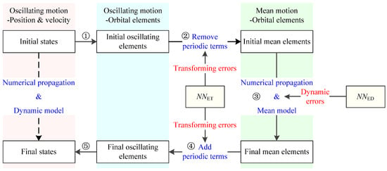
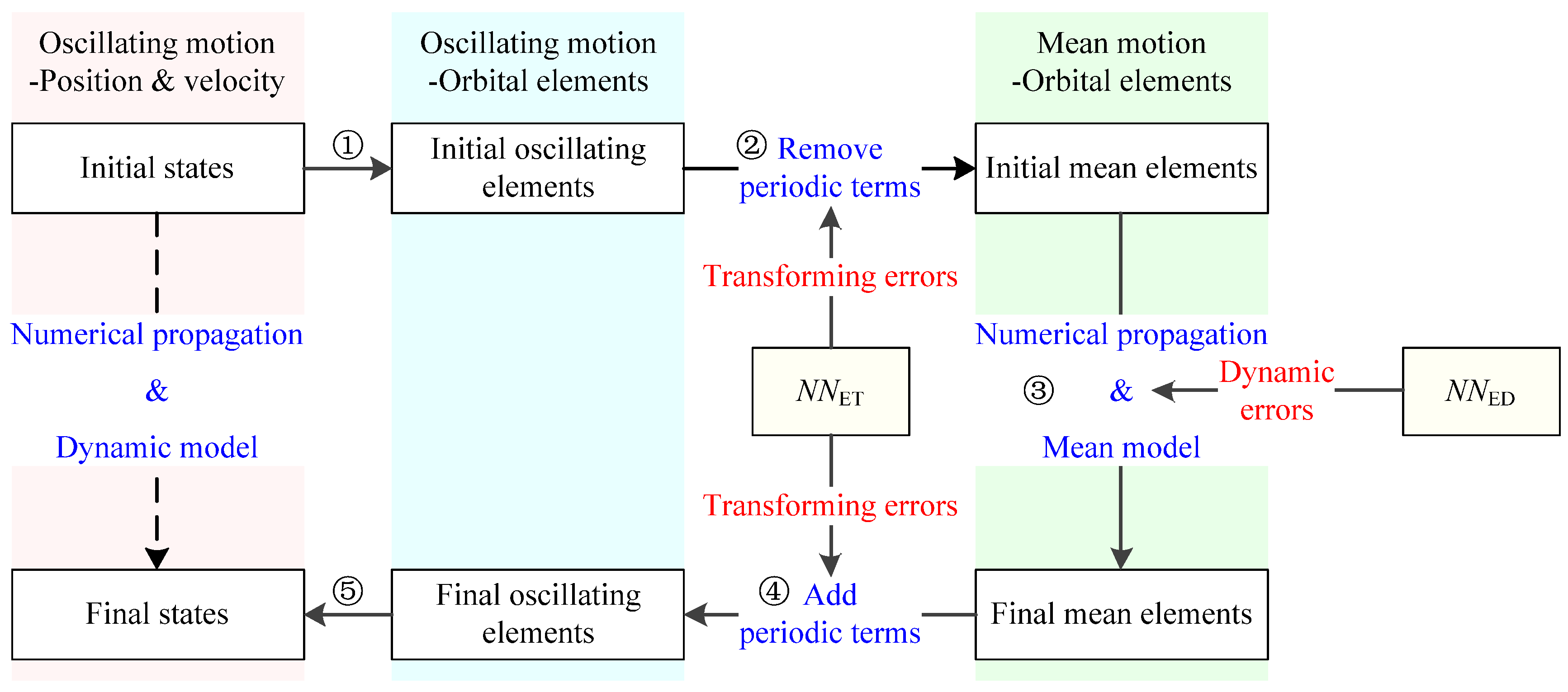
In this section, the propagation method for IGSO with respect to the mean non-singular orbital elements is developed. The propagation of the IGSO is essentially a problem of solving a system of differential equations. The differential equations are the mean rates of change of the non-singular elements, while the initial conditions are the initial oscillating states, i.e., the position and velocity vectors, of the IGSO satellite. The integration is performed over the time interval. In order to match the initial oscillating states and the mean models, the propagation method for the IGSO is shown in Figure 1 and in the following steps:

Figure 1. Orbit propagation for IGSO.

(1) The initial oscillating states of the IGSO are transformed into the non-singular oscillating orbital elements;

(2) The oscillating elements are transformed into the mean elements by removing the periodic terms of the IGSO;

(3) The initial mean elements are propagated to obtain the final mean elements of the IGSO based on the mean dynamic models;

(4) The final mean elements are transformed into the final oscillating elements by adding the periodic terms;

(5) The final oscillating elements are transformed into the final states of the IGSO.

According to Section 3, because the simplifications and truncations are intended to isolate the short-period terms and derive the mean models, errors arise in the transformations and the mean dynamic models. In this situation, an accurate mean model ${\overline{\dot{\zeta }}}^{\prime }$ considering the mean dynamic errors on the IGSO is shown as follows:

$${\overline{\dot{\zeta }}}^{\prime }=\overline{\dot{\zeta }}+{\overline{\dot{\zeta }}}_{\mathrm{ED}}$$

(39)

where the subscript ED represents the errors on the mean dynamic model.

Meanwhile, an accurate transformation model ζ^′ considering the short-period term errors on the IGSO is shown as follows:

$${\zeta }^{\prime }={\overline{\zeta }}^{\prime }+\Delta {\zeta }_{\mathrm{SP}}+\Delta {\zeta }_{\mathrm{SP},\mathrm{ET}}$$

(40)

where the subscript ET represents the short-period term errors on the transformation.

The propagation of the IGSO becomes

$${\zeta }^{\prime }={\displaystyle \int \left(\overline{\dot{\zeta }}+{\overline{\dot{\zeta }}}_{\mathrm{ED}}\right)\mathrm{d}t}+\Delta {\zeta }_{\mathrm{SP}}+\Delta {\zeta }_{\mathrm{SP},\mathrm{ET}}$$

(41)

The corresponding models and errors of the propagation are summarized in Table 1. The analytical models for orbital propagation are the mean rates of change of the non-singular elements, while the analytical models for transformation are the short-period terms. The errors mainly consist of the high-order terms of the non-spherical gravitations of the Earth, the high-order truncations of the gravitations and solar radiation pressure including eclipses, Earth shadowing, the coupled effects of the non-singular elements, the evolution of the latitude and other perturbations including solid Earth tides, ocean tides and relativity. These errors are fitted and predicted using neural networks.

Table 1. Models and errors for orbit propagation and transformation.

Item	Propagation	Transformation
Analytical Models	(14)(20)(27)(33)	(17)(23)(30)(36)
Errors of non-spherical gravitation of the Earth	High-order mean terms, simplification and truncation of the geocentric distance	High-order short-period terms, simplification and truncation of the geocentric distance
Errors of luni-solar gravitations	Simplifications and truncations of the luni-solar mean distances	Simplifications and truncations of the luni-solar angles
Errors of solar radiation pressure	Simplification of the solar distance, eclipses and Earth shadowing	Simplification of the solar angle, eclipses and Earth shadowing
Others	Coupled effects of mean orbital elements, latitude evolution, other perturbations	Coupled effects of short-period terms, latitude evolution, other perturbations

4.2. NN-Based Error Prediction Method

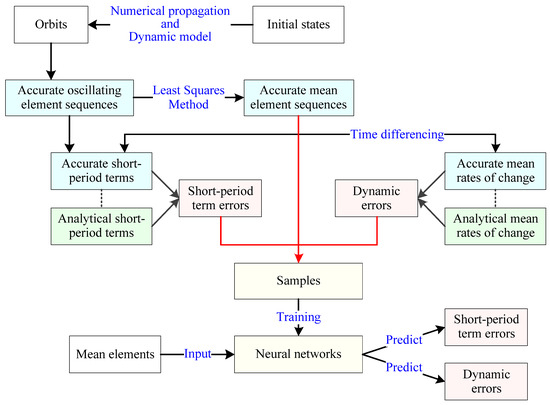
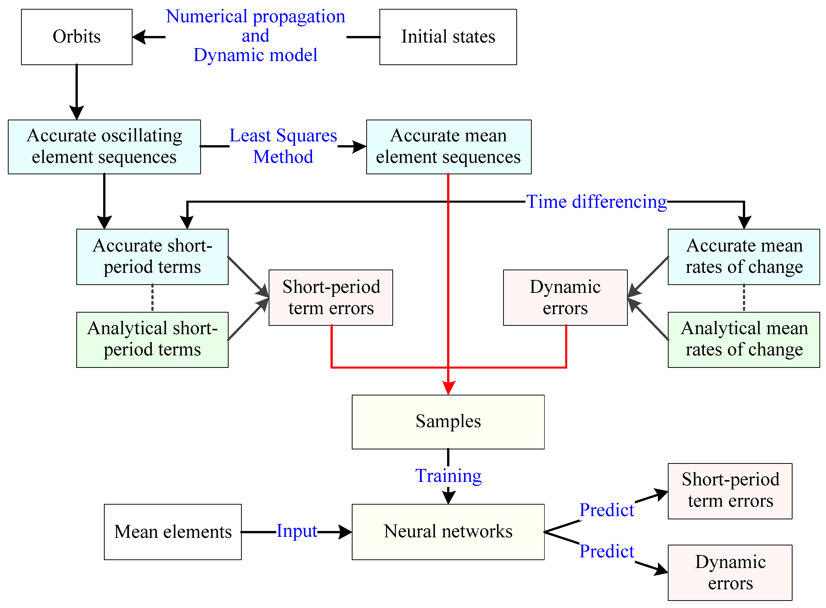
Due to the errors in transformation and propagation, the propagated IGSO significantly deviates from the actual orbit. In order to improve the orbit accuracy, neural networks are employed to fit and predict the errors of the short-period terms and the mean dynamic models. Considering the different roles of the mean dynamic model in orbit propagation and the transformation model in obtaining the oscillating states, two separate neural networks are used to predict the propagation and transformation errors. The NN-based error prediction method is shown in Figure 2. The inputs of both networks are the current date and the non-singular elements. The outputs are short-period term errors and dynamic errors. Furthermore, note that the present study mainly concentrates on a general prediction method for neutralizing the errors of the short-period terms and the mean dynamic models, in which common neural networks can be adopted.

Figure 2. NN-based error prediction method.

• The neural network-based error prediction method is described as follows:

(1) Set the initial date, position and velocity as initial states for the IGSO satellite. The IGSO is propagated based on the accurate dynamic model through numerical propagation. The sequences of dates, positions and velocities of the orbit are decomposed. To guarantee the accuracy, small values should be chosen as the time steps for the sequences. Then, the accurate oscillating element sequences for the IGSO are obtained.

(2) Based on the least-squares method, the accurate oscillating element sequences are smoothed, and the short-period terms are removed. The accurate mean element sequences with respect to the non-singular elements are extracted.

(3) The accurate short-period terms are calculated by subtracting the accurate mean elements from the accurate oscillating elements. Then, together with the analytical short-period terms derived in the present paper, the short-period term errors are collected.

(4) Similar to step (3), the accurate mean rates of change of the non-singular elements are solved based on a time differencing method. The mean dynamic errors are collected using the accurate and analytical (provided in the present paper) rates of change.

(5) The date, accurate mean elements, errors in the short-period terms and dynamic errors are grouped into a sample. By iterating Steps (1)–(5), a set of IGSO samples containing mean elements and errors is created.

(6) The set of samples is employed to train the neural networks.

For the dynamic error prediction network, the inputs are the date and the non-singular elements [a,e_x,e_y,i_x,i_y,L] of the IGSO, while the output is the error of the mean dynamic model ${\overline{\dot{\zeta }}}_{\mathrm{ED}}$, which is given as follows:

$${\overline{\dot{\zeta }}}_{\mathrm{ED}}=N{N}_{\mathrm{ED}}\left(\mathit{JD},a,e_x,e_y,i_x,i_y,L\right)$$

(42)

where JD represents the date, which is employed to indirectly introduce the ephemerides of the Sun and the Moon in the networks. In this study, the Julian date is adopted.

For the short-period term error prediction network, the errors of the short-period terms are combined and denoted by a parameter Δζ_SP,ET. In this situation, the inputs are the date JD and the non-singular elements [a,e_x,e_y,i_x,i_y,L] of the IGSO, while the output is the error of the short-period terms Δζ_SP,ET, which is given as follows:

Δζ_SP,ET = NN_ET(JD,a,e_x,e_y,i_x,i_y,L)

(43)

(7) After the training, the dynamic error prediction network and the short-period term error prediction network are employed to correct the models in the orbit propagation and transformation of the IGSO.

It should be emphasized that the transforming models require the ephemerides of the Sun and the Moon. Accurate ephemerides are aperiodic, which cannot be replaced by simplified models. Therefore, during the training of both networks, the Julian date JD should cover the whole mission duration of the IGSO satellite to mitigate the effects of time-varying ephemerides. Moreover, the short-period term and mean dynamic errors contain high order coupled terms, solar radiation pressures and other perturbations.

The performance of the NN-based error prediction method and the intelligent propagation method for the IGSO is validated in the next section.

5. Numerical Simulation

5.1. Initial Conditions for Simulation

In this section, the intelligent propagation method is studied through numerical simulations. The accuracy of the intelligent transformation method between the mean and oscillating elements is first validated. Then, the performance of the intelligent propagation method for the IGSO is analyzed. The dynamic models for numerical simulations and the initial conditions of the IGSO are provided.

Four models listed in Table 2 are built to simulate the motions of the IGSO satellite: (1) A high-accuracy model considers the gravitations of the Earth (up to 21 orders of non-spherical terms), the Sun and the Moon, and the solar radiation pressure. The orbit is propagated using oscillating states, and the mean elements are calculated based on the least-squares method. (2) A GEO model includes the gravitation of the Earth (up to 4 orders of non-spherical terms), the Sun and the Moon, and the solar radiation pressure. The orbit is propagated using mean elements. A typical transformation model for the GEO satellite is taken as a reference. (3) A simplified model combines the gravitations of the Earth (up to 4 orders of non-spherical terms), the Sun and the Moon, and the solar radiation pressure. The orbit is propagated using mean elements. The analytical transformation model is taken as the transformation model. (4) An NN-based model is built on the simplified model and extended with deep neural networks to predict and neutralize the dynamic error and short-period term error. A Runge–Kutta 8(7) solver with adaptive step size is employed as the integrator. Tolerances are set as 10⁻¹³.

Table 2. Dynamics and methods for simulation.

Models	High-Accuracy	GEO	Simplified	NN-Based
Gravitations	Earth’s gravity (21 orders), Solar gravity, Lunar gravity	Earth’s gravity (4 orders), Solar gravity, Lunar gravity	Earth’s gravity (4 orders), Solar gravity, Lunar gravity	Earth’s gravity (4 orders), Solar gravity, Lunar gravity
Solar radiation pressure	Included	Included	Included	Included
Propagation	Oscillating	Mean	Mean	Mean
Transformation	Least squares	GEO model [12]	Simplified model	Simplified model
Error prediction				Deep neural network

The IGSO is used as an example for validation. The mission period is set from 1 January 2027 (JD 2,461,406.5) to 1 January 2028 (JD 2,461,771.5). The IGSO satellite is located in the geosynchronous orbit with an orbital period equal to the sidereal day of the Earth (86,164.09 s). The initial conditions for sampling are listed in Table 3. Considering a typical IGSO satellite, the range of the inclination is set to 0–60 deg, while the ranges of the RAAN, the argument of perigee and the true anomaly are 0–360 deg. The samples are generated accordingly. Referring to the station-keeping cycles of current GEO and IGSO satellites in practical missions, the time span of propagation is set to 7 days (604,800 s).

Table 3. Sample conditions.

Item	Value	Unit
Date	2,461,406.5–2,461,771.5	JD
Period	86,164.09	sec
Eccentricity	10−3
Inclination	0–60	deg
RAAN	0–360	deg
Argument of perigee	0–360	deg
True anomaly	0–360	deg
Time span	7	days

Subject to the above conditions, 1000 IGSOs are generated. Each orbit is split into 865 samples, with a time step of 100 s. Following Section 4.2, the mean elements, short-period terms and corresponding errors are calculated. The results are grouped into 865,000 samples for network training. The Matlab 2024b software is employed to construct the networks. A deep feedforward neural network with 4 hidden layers containing 24 nodes each is introduced to predict the mean dynamic error; while for the short-period term error prediction, a deep feedforward neural network with 4 hidden layers containing 32 nodes each is deployed. The ReLU is set as the activation functions. The Adam method is set as the optimizer. Learning rate is set as 0.001. The mean squared error loss function (MSELoss) is set as the loss function. The number of epochs is set as 500, and the training is stop when the validation accuracies do not improve for 10 consecutive epochs. The batch size is set as 32. The Multi-Specialty Recruitment Assessment (MSRA) is chosen for initialization. The BatchNorm is used for normalization, while the Dropout method is used for regularization. The random seed is not specified. During the training of both networks, 90% of the samples are randomly selected as training sets, 5% as validation sets and 5% as test sets, thereby allowing the networks to fully map sample space.

It takes about 267 epochs (about 44.31 h) and 244 epochs (about 41.96 h) for training the mean dynamic error prediction network and the short-period term error prediction network, respectively.

After the networks are trained, two cases are taken to verify the intelligent transformation and propagation methods. The initial conditions of these two cases are provided in Table 4. Case A refers to the ISRO-NavIC satellite with an inclination of 30°, while case B refers to the BDS-IGSO satellite with an inclination of 55°. Other elements are selected randomly according to the conditions in Table 3.

Table 4. Initial conditions for two cases.

Item	Case A	Case B	Unit
Date	2,461,406.5	2,461,406.5	JD
Period	86,164.09	86,164.09	sec
Eccentricity	10−4	1e−4
Inclination	30	55	deg
RAAN	210	30	deg
Argument of perigee	50	60	deg
True anomaly	240	120	deg
Time span	7	7	days

5.2. Validation of NN-Based Transformation

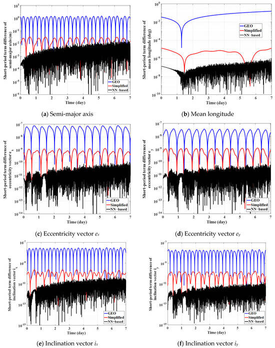
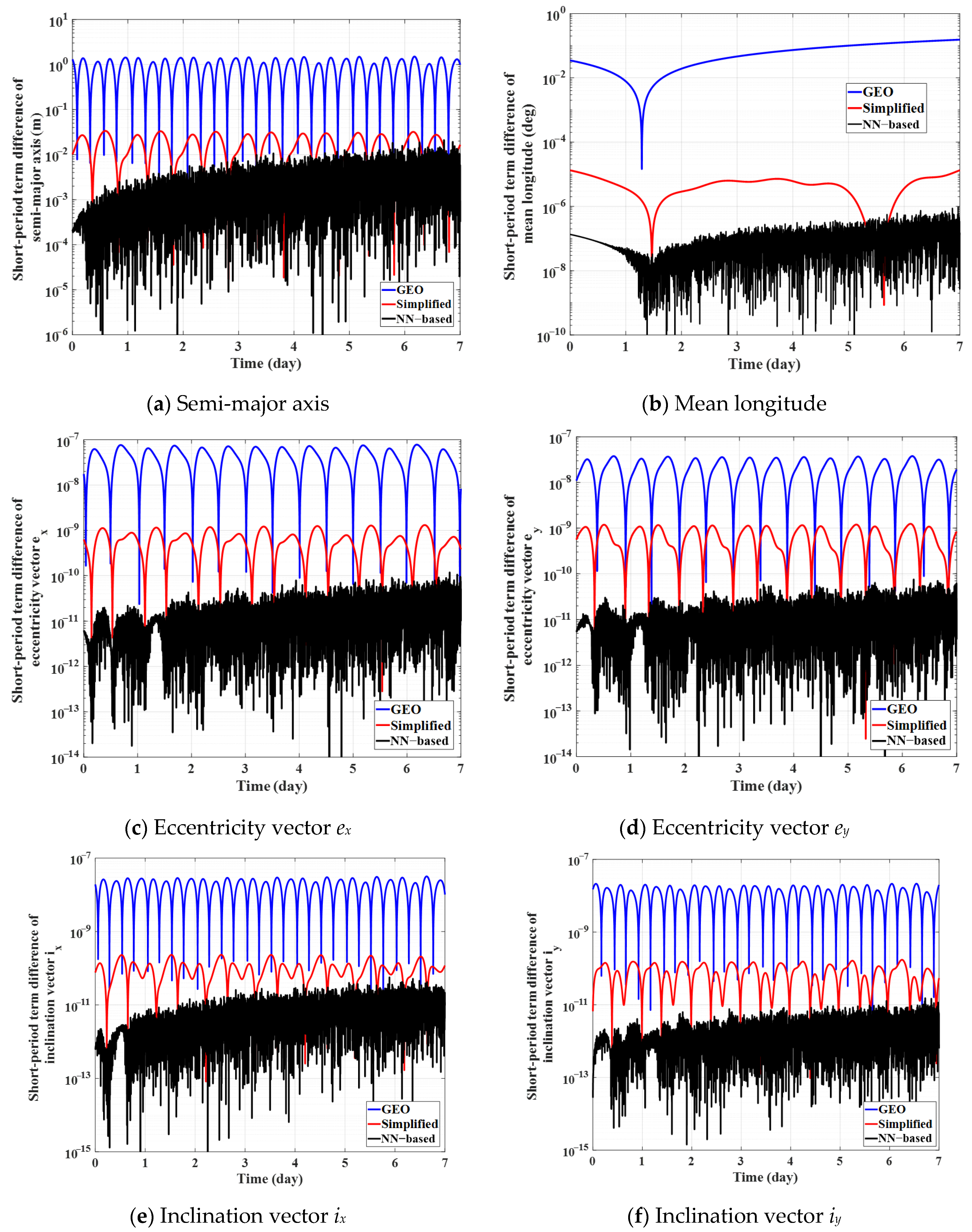
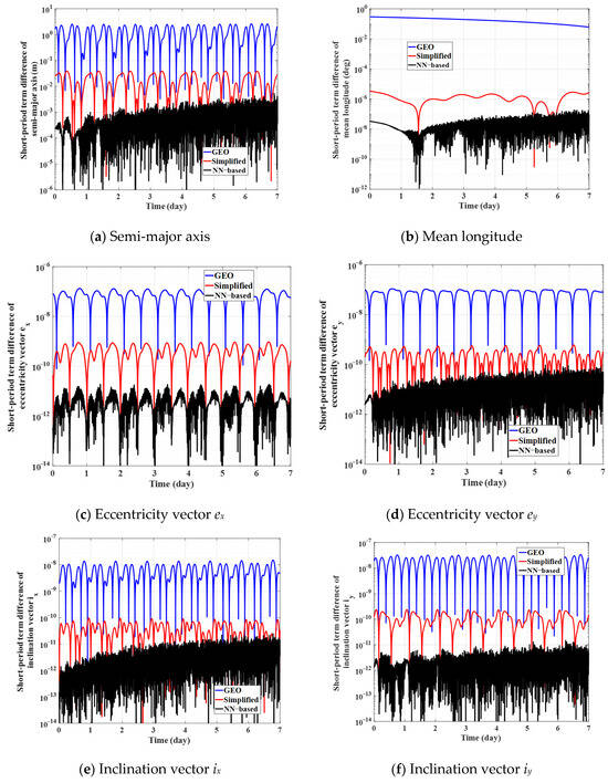
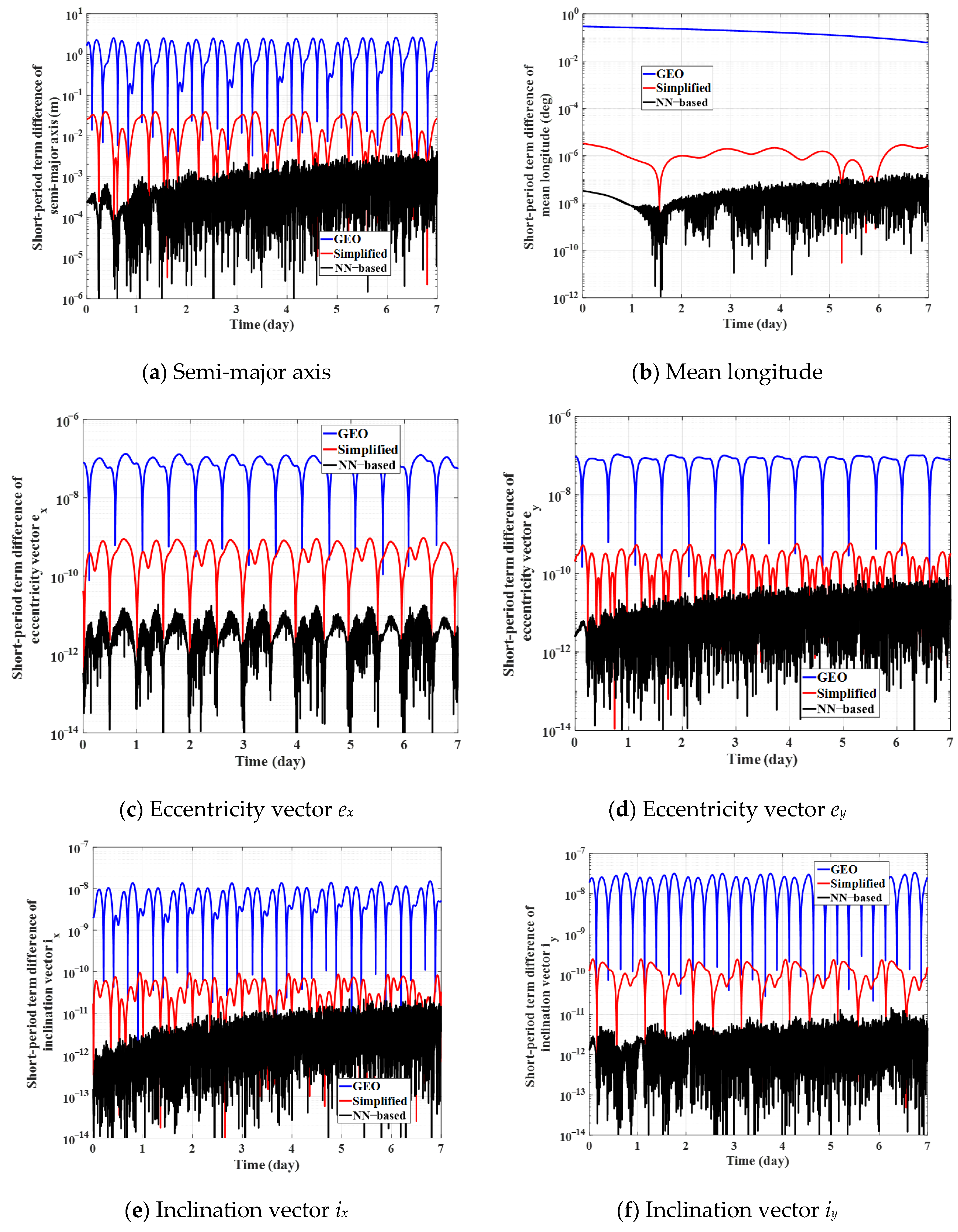
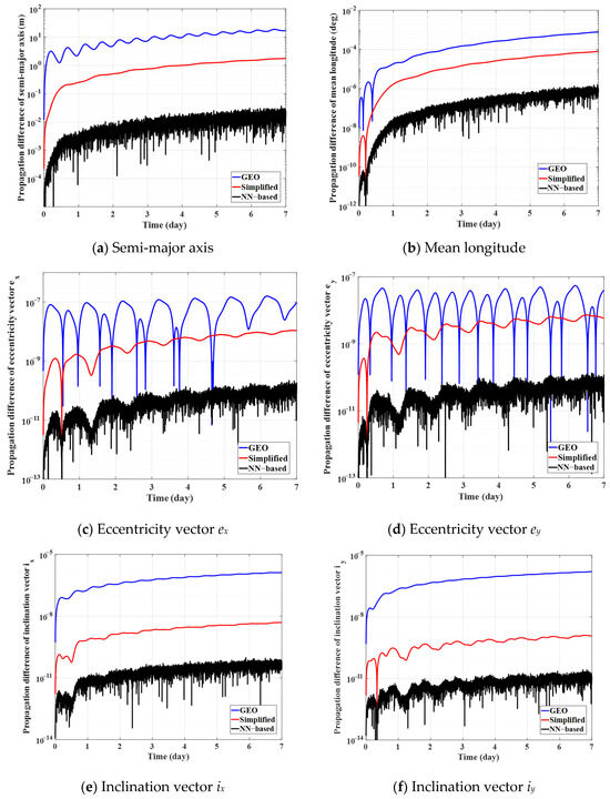
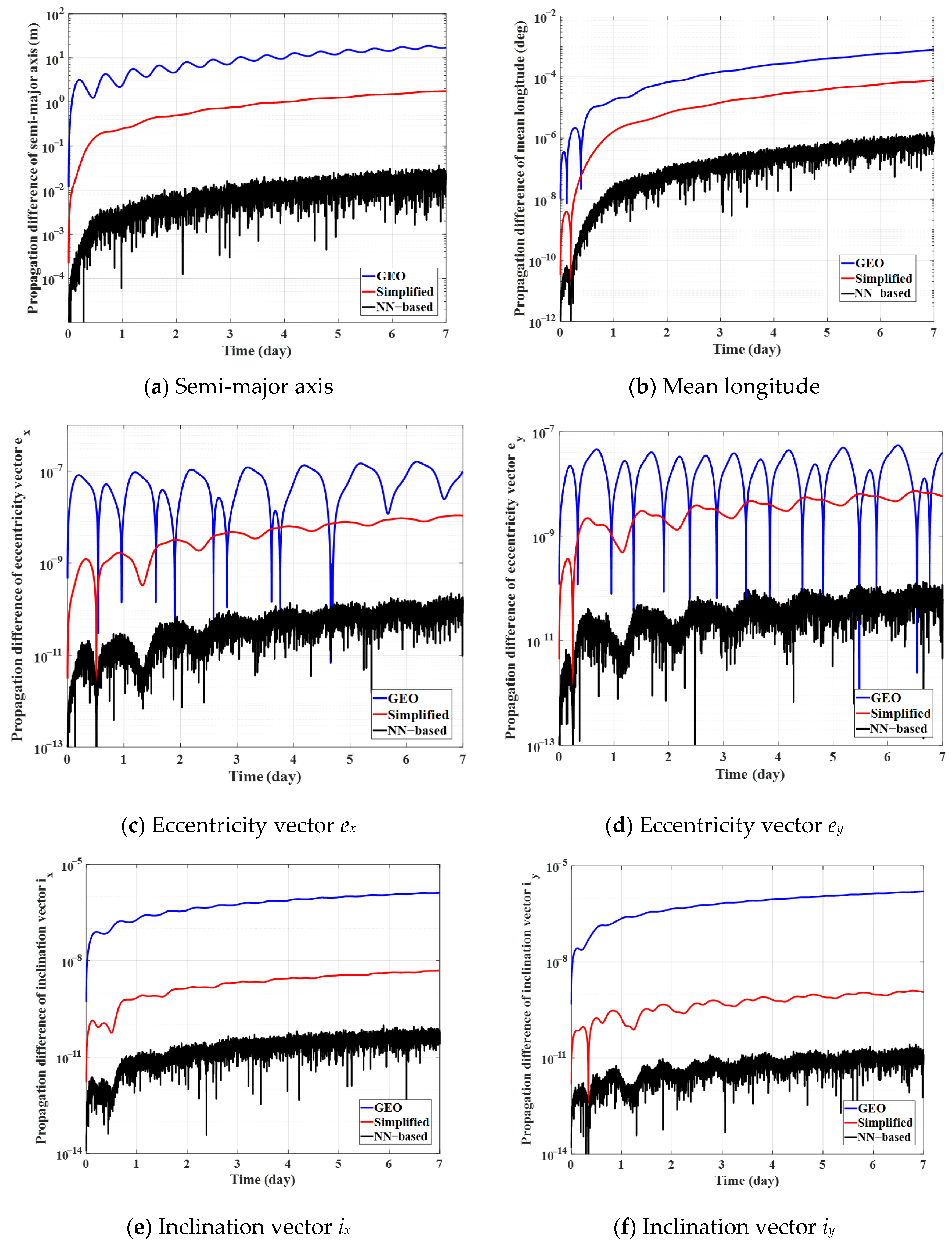
The accuracy of NN-based transformations between the mean and oscillating elements is first validated. The initial conditions are provided in Table 2 and Table 4. During the simulations, the orbits of the two cases are propagated based on the high-accuracy model. The accurate short-period terms are calculated. Then, by inputting the mean non-singular elements into the short-period term error prediction network, the relevant NN-based short-period terms are obtained. In addition, the short-period terms of the GEO model and simplified model are calculated for comparison. With the accurate short-period terms as baseline, the differences in the non-singular elements with respect to the NN-based model, the GEO model and the simplified model are provided in Figure 3 and Figure 4.

Figure 3. Short-period term differences of case A (i = 30°).

Figure 4. Short-period term differences of case B (i = 55°).

According to the case A orbits in Figure 3, the errors of the non-singular elements of the simplified model are about 2 orders of magnitude smaller than those of the GEO model. This suggests that the motion of the inclination has a significant influence on the short-period terms of the IGSO, which should be considered to reduce the transformation errors. Then, the orders of magnitude of the short-period term errors of the NN-based model are approximately 10⁻³ m, 10⁻⁷ °, 10⁻¹¹, 10⁻¹¹, 10⁻¹¹, 10⁻¹², with respect to the semi-major axis, the mean longitude, the eccentricity vector e_x, the eccentricity vector e_y, the inclination vector i_x and the inclination vector i_y, respectively. Moreover, the errors of the simplified model are approximately periodic, while those of the NN-based model are combinations of periodic errors and random errors. Meanwhile, the errors of the short-period terms appear to diverge slightly over time. These indicate that the periodic errors are dominant terms. The time-related non-periodic terms (caused by luni-solar gravitations and solar radiation pressure) are secondary terms. The deep neural network mainly fits and neutralizes the periodic errors to improve the transformation accuracy.

From the case B orbits in Figure 4, due to a higher inclination, the differences in the short-period terms based on the GEO model are rather large, especially for the mean longitude (which is about three orders of magnitude larger than that of the simplified model). Similar to the case A orbits, the NN-based model guarantees the accuracy of the short-period terms. The orders of magnitude of the short-period term errors of the NN-based model are about 10⁻³ m, 10⁻⁷ °, 10⁻¹¹, 10⁻¹¹, 10⁻¹¹, 10⁻¹², with respect to the semi-major axis, the mean longitude, the eccentricity vector e_x, the eccentricity vector e_y, the inclination vector i_x and the inclination vector i_y, respectively.

The simulation results of cases A and B verify that the proposed NN-based short-period term prediction method can fit and predict the transformation errors with high accuracy. The short-period term errors of the semi-major axis of the NN-based model are about one and three orders of magnitude smaller than those of the simplified model and GEO model, respectively. Meanwhile, the short-period term errors of the mean longitude, the eccentricity vectors and the inclination vectors of the NN-based model are about two and four orders of magnitude smaller than those of the simplified model and GEO model, respectively. Therefore, the NN-based transformation method achieves high transformation accuracy between the mean element and oscillating elements with respect to the IGSO.

5.3. Analysis of Intelligent Propagation Method

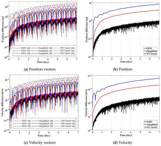
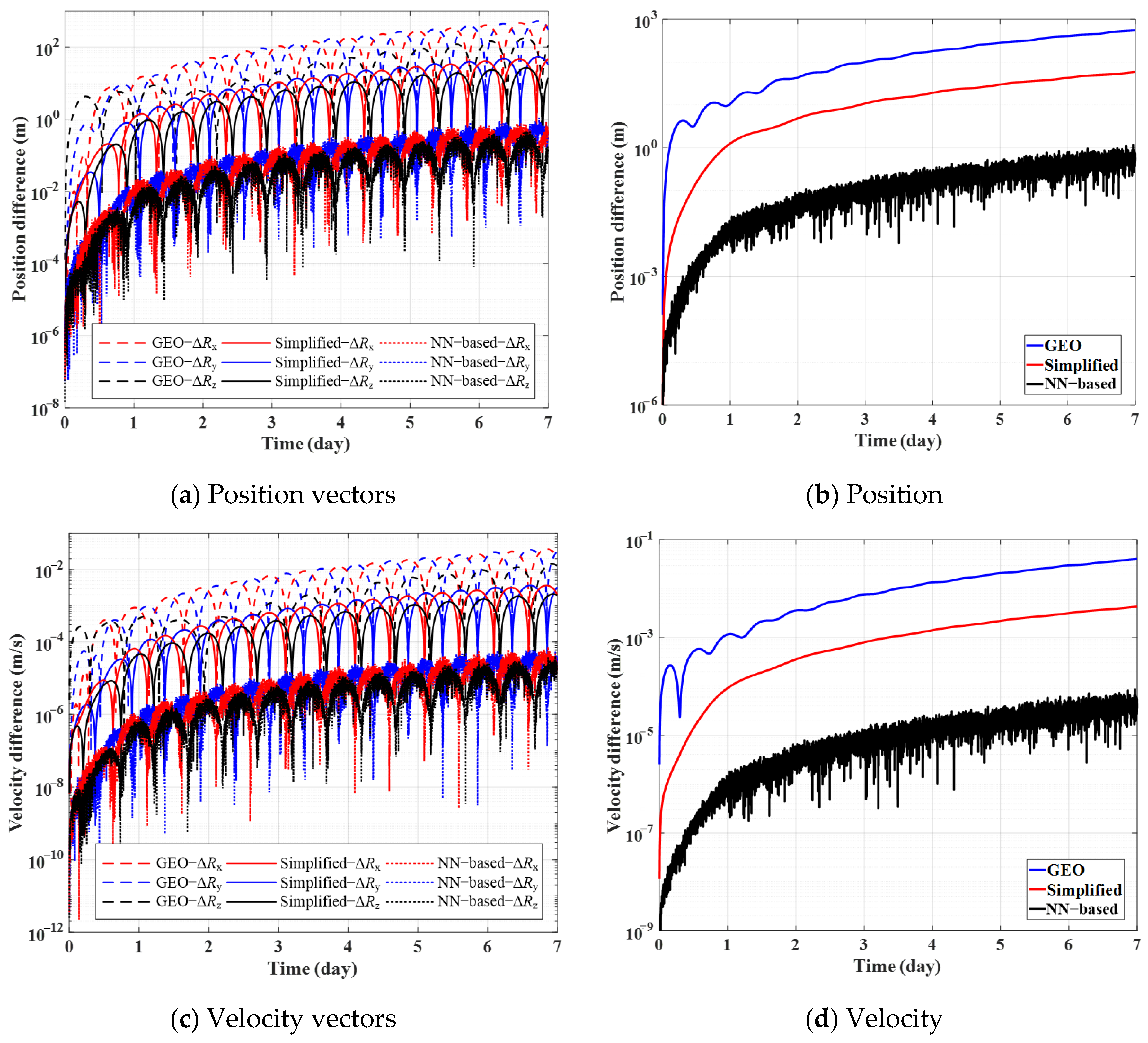
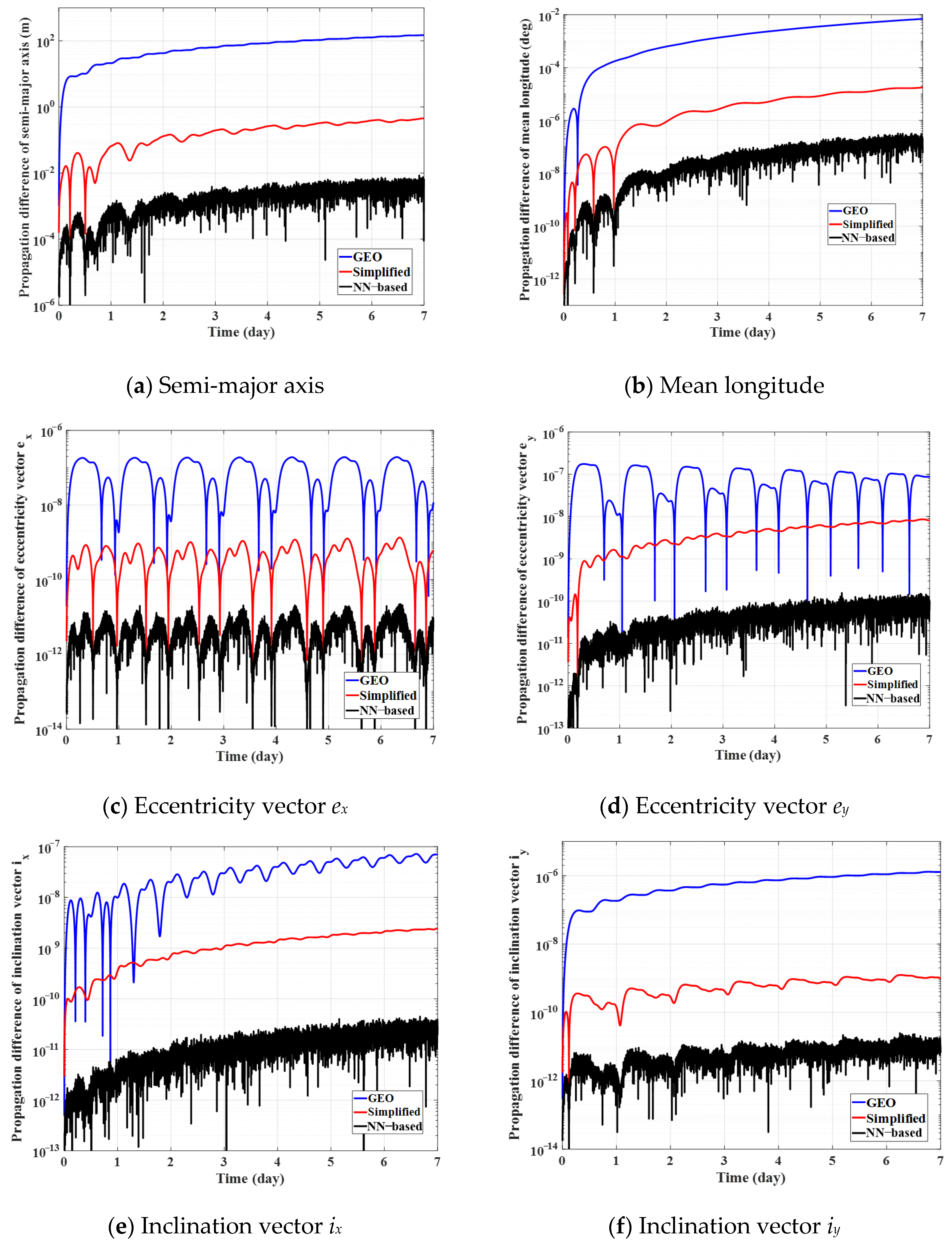
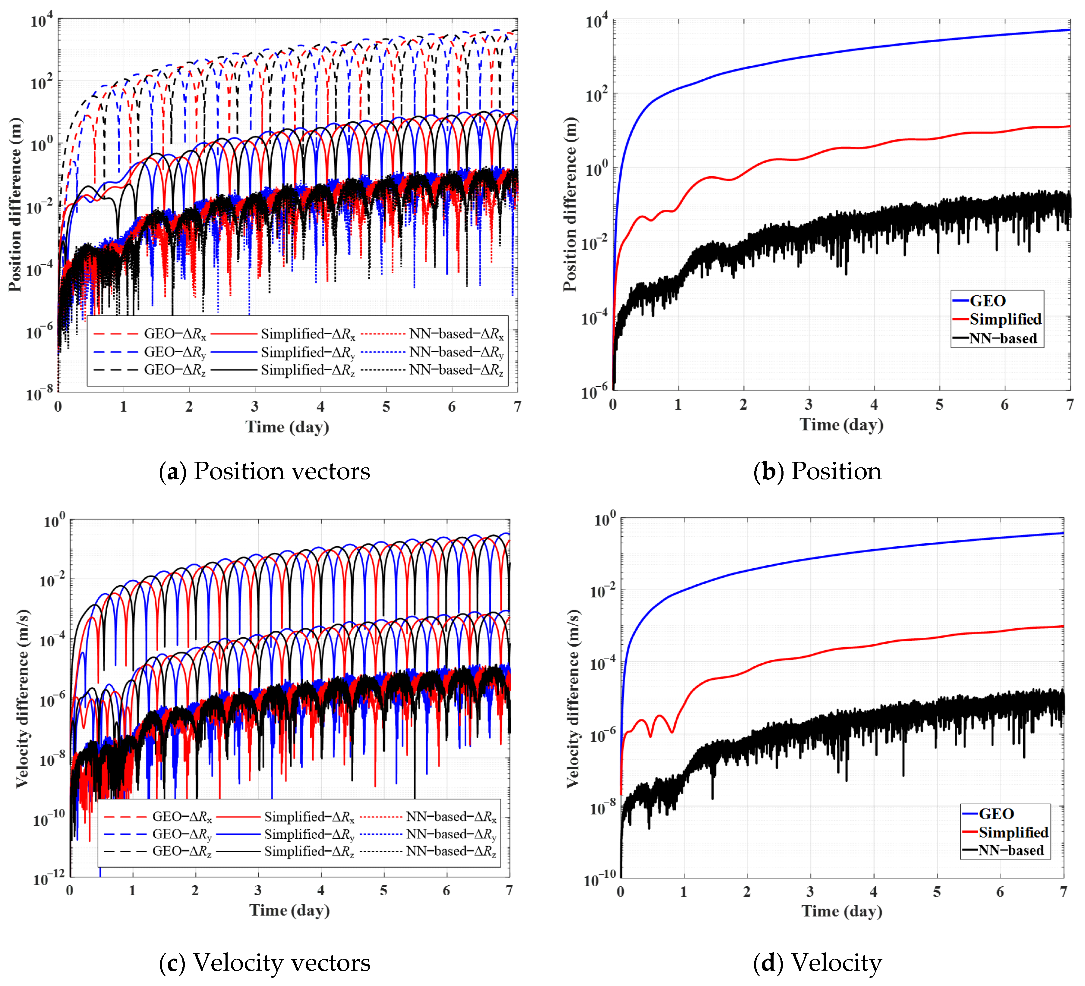
In the second simulation, the performance of the intelligent propagation method for the IGSO is analyzed. The initial conditions are provided in Table 2 and Table 4. The orbits of the two cases are propagated based on the high-accuracy model and oscillating elements. The initial mean elements are solved accordingly. Then, the orbits are propagated, with respect to the mean elements using the GEO model, the simplified model and the NN-based model. The mean elements are transformed into oscillating elements for difference analysis. During each propagation, the mean elements of the IGSO are input into the dynamic error prediction network to obtain the errors of mean rates of change of the IGSO. With the high-accuracy orbit as the baseline, the differences in non-singular elements and states obtained using the NN-based model, the GEO model and the simplified model are shown in Figure 5, Figure 6, Figure 7 and Figure 8.

Figure 5. Propagation differences of case A (i = 30°).

Figure 6. Position and velocity differences of case A (i = 30°).

Figure 7. Propagation differences of case B (i = 55°).

Figure 8. Position and velocity differences of case B (i = 55°).

According to the case A orbits in Figure 5, due to the dynamic errors, the differences in the simplified model are about one order (semi-major axis, mean longitude and eccentricity vectors) and two orders (inclination vectors) of magnitude smaller than those with respect to the GEO model. This demonstrates that the inclination significantly affects the secular evolution of the IGSO. In this situation, the effect of the inclination should be considered. Then, the orbit differences in the NN-based model are about 10⁻² m, 10⁻⁶ °, 10⁻¹⁰, 10⁻¹⁰, 10⁻¹¹, 10⁻¹¹ with respect to the semi-major axis, the mean longitude, the eccentricity vector e_x, the eccentricity vector e_y, the inclination vector i_x and the inclination vector i_y, respectively. Furthermore, in association with Figure 3, the differences in the non-singular elements are composed of secular drifts and periodic oscillations. The secular drift tendencies with respect to the simplified model and the NN-based model are similar. The magnitude of the dynamic errors is smaller than that of the short-period terms. Meanwhile, the secular drifts gradually dominate the periodic oscillations over time. Therefore, the dynamic errors in the mean rates of change should be fitted and predicted using an independent network to improve the propagation accuracy.

As shown in Figure 6, by neutralizing the dynamic errors using a deep neural network, the NN-based method shows the highest position and velocity accuracies among the three models. Over a 7-day mission, the magnitude of the position difference is approximately 1 m, which is two and three orders of magnitude smaller than the corresponding values obtained using the simplified and GEO models, respectively. The magnitude of the velocity difference is approximately 10⁻⁴ m/s, which is likewise two and three orders of magnitude smaller.

As shown by the case B results in Figure 7, due to a high inclination, the differences with respect to the GEO model drift significantly, which makes it inappropriate for the IGSO. The differences in the simplified model are about two orders of magnitude smaller than those of the GEO model. The orbit differences in the NN-based model are about 10⁻² m, 10⁻⁷ °, 10⁻¹¹, 10⁻¹⁰, 10⁻¹¹, 10⁻¹¹ with respect to the semi-major axis, the mean longitude, the eccentricity vector e_x, the eccentricity vector e_y, the inclination vector i_x and the inclination vector i_y, respectively. Similar to case A, in association with Figure 4, although the values are smaller, the accumulated dynamic errors dominate the short-period terms over time. In this situation, the introduction of the deep neural network for correcting the dynamic errors is essential.

Figure 8 shows that in a 7-day mission, the position difference is about 0.1 m in magnitude (two orders and three orders of magnitudes lower than the simplified model and GEO model), while the velocity difference is about 10⁻⁵ m/s in magnitude (two and three orders of magnitude lower than the simplified model and GEO model, respectively). The accuracies in position and velocity are higher than those of case A orbit. This is because the high inclination prevents the motions of the mean longitude and the inclination vectors from approaching singularities.

In order to further analyze the performance of the proposed NN-based propagation method, a large test set with 500 samples is employed. The samples are generated according to the initial conditions in Table 3, with propagation time of 7 days. The errors in distance of final states are taken to evaluate the propagating accuracy. The results including averaged error, RMS, maximum error, median error and computation time are shown in Table 5. From Table 5, for the NN-based method, the averaged error is about 2.139 × 10⁻¹ m, which is 4 orders of magnitude smaller than that of the GEO model. The RMS, maximum error and median error with respect to the NN-based method are improved compared to the GEO model and simplified model. The computation times of the NN-based model are about 85.90 s which is about 18.932% of the computation time of the high-accuracy model.

Table 5. Propagation performances.

Models	High-Accuracy	GEO	Simplified	NN-Based
Averaged error (m)	-	6.757 × 103	9.263 × 101	2.139 × 10−1
RMS (m)	-	9.615 × 103	1.512 × 102	3.377 × 10−1
Maximum error (m)	-	1.128 × 104	1.663 × 102	3.652 × 10−1
Median error (m)	-	7.183 × 103	1.088 × 102	2.397 × 10−1
Computation time (sec)	453.71	12.66	20.03	85.90

The simulation results of cases A and B verify the performance of the proposed intelligent propagation method for an IGSO. The propagation errors in the non-singular elements and the position and velocity of the NN-based model are about two orders of magnitude smaller than those obtained using the simplified model. Therefore, the proposed intelligent propagation method achieves high secular propagation accuracy for the IGSO with a short computation time.

6. Conclusions

The intelligent propagation at an inclined geosynchronous orbit (IGSO) using mean elements is studied. The states of the IGSO satellite are transformed into mean elements, propagated over the long-term using the mean dynamic model and then transformed back into oscillating elements. The orbital perturbations including four orders of zonal harmonics terms and tesseral harmonics terms of the Earth’s gravitation, luni-solar gravity and solar radiation pressure are considered. The mean terms and short-period terms of the IGSO are isolated using the averaging method. The analytical transformation method between the mean and the oscillating elements of the IGSO is constructed. Based on the IGSO propagation, the sources of propagation and transformation errors are analyzed. The propagation errors mainly arise from high-order truncation in the derivation and the coupled effects of the mean motions which are summarized as mean dynamic errors. The transformation errors are attributed to the high-order coupled effects of periodic terms and the ephemeris which are collectively referred to as short-period term errors. These strong linear errors of short-period terms and mean dynamic models are neutralized using two separate deep neural networks.

Numerical simulations show that, by fitting and predicting the short-period term errors and mean dynamic errors using deep neural networks, the proposed intelligent propagation method improves the accuracy of transformation and propagation for the IGSO. For the transformation between mean and oscillating elements, compared to the simplified model, the NN-based method achieves improvements in accuracies of one order (semi-major axis) and two (mean longitude, eccentricity vectors and inclination vectors) orders of magnitudes. For the IGSO propagation, the NN-based method achieves improvements in accuracies of one order (semi-major axis, mean longitude and eccentricity vectors) and two orders (inclination vectors) of magnitudes. Over a 7-day mission, the position and velocity differences obtained using the intelligent propagation method are approximately 0.1 m and 10⁻⁵ m/s, respectively. These values are approximately two orders of magnitude smaller than those obtained using the simplified model. Moreover, since that the present study maps the short-period term and mean dynamic errors with the Julian date and non-singular elements using deep neural networks, the transferabilities of the networks depends on the training samples. Therefore, in order to expand the applicable range of the NN-based method, the samples should cover the possible ranges of Julian date and orbital parameters.

References

- Fantino, E.; Flores, R.M.; Di Carlo, M.; Cabot, E. Geosynchronous inclined orbits for high-latitude communications. Acta Astronaut. 2017, 140, 570–582. [Google Scholar] [CrossRef] [Scilit]
- Zhou, S.S.; Hu, X.G.; Wu, B.; Liu, L.; Qu, W.; Guo, R.; He, F.; Cao, Y.; Wu, X.; Zhu, L.; et al. Orbit determination and time synchronization for a GEO/IGSO satellite navigation constellation with regional tracking network. Sci. China Phys. Mech. Astron. 2011, 54, 1089–1097. [Google Scholar] [CrossRef] [Scilit]
- Santra, A.; Mahato, S.; Dan, S.; Bose, A. Precision of satellite based navigation position solution: A review using NavIC data. J. Inf. Optim. Sci. 2019, 40, 1683–1691. [Google Scholar] [CrossRef] [Scilit]
- Gao, W.; Zhou, W.; Tang, C.; Li, X.; Yuan, Y.; Hu, X. High-precision services of BeiDou navigation satellite system (BDS): Current state, achievements, and future directions. Satell. Navig. 2024, 5, 20. [Google Scholar] [CrossRef] [Scilit]
- Steigenberger, P.; Hugentobler, U.; Hauschild, A.; Montenbruck, O. Orbit and clock analysis of Compass GEO and IGSO satellites. J. Geod. 2013, 87, 515–525. [Google Scholar] [CrossRef] [Scilit]
- Li, L.; Colombo, C.; Gkolias, I.; Zhang, J. Low-thrust station-keeping towards exploiting the inclined geosynchronous dynamics. Adv. Space Res. 2023, 72, 1570–1582. [Google Scholar] [CrossRef] [Scilit]
- Tang, J.; Hou, X.; Liu, L. Long-term evolution of the inclined geosynchronous orbit in Beidou Navigation Satellite System. Adv. Space Res. 2017, 59, 762–774. [Google Scholar] [CrossRef] [Scilit]
- Huang, X.; Masdemont, J.J.; Li, S. Dynamic analysis of Europa probe considering J2 perturbation of Jupiter. J. Guid. Control Dyn. 2024, 47, 156–164. [Google Scholar] [CrossRef] [Scilit]
- Dong, X.; Hu, C.; Long, T.; Li, Y. Numerical analysis of orbital perturbation effects on inclined geosynchronous SAR. Sensors 2016, 16, 1420. [Google Scholar] [CrossRef] [Scilit] [PubMed]
- Jenkin, A.B.; McVey, J.P.; Sorge, M.E. Assessment of time spent in the LEO, GEO, and semi-synchronous zones by spacecraft on long-term reentering disposal orbits. Acta Astronaut. 2022, 193, 579–594. [Google Scholar] [CrossRef] [Scilit]
- Zhao, C.Y.; Zhang, M.J.; Wang, H.B.; Xiong, J.N.; Zhu, T.L.; Zhang, W. Analysis on the long-term dynamical evolution of the inclined geosynchronous orbits in the Chinese BeiDou navigation system. Adv. Space Res. 2015, 56, 377–387. [Google Scholar] [CrossRef] [Scilit]
- Shen, H.X.; Kuai, Z.Z.; Li, H.N. Propagation and transformation of mean elements at geostationary orbits. J. Guid. Control Dyn. 2019, 42, 2132–2142. [Google Scholar] [CrossRef] [Scilit]
- Soop, E.M. Handbook of Geostationary Orbits; Springer Science & Business Media: Dordrecht, The Netherlands, 1994. [Google Scholar]
- Celletti, A.; Galeş, C.; Pucacco, G.; Rosengren, A.J. Analytical development of the lunisolar disturbing function and the critical inclination secular resonance. Celest. Mech. Dyn. Astron. 2017, 127, 259–283. [Google Scholar] [CrossRef] [Scilit]
- Tan, P.; Tang, J.S.; Hou, X.Y. Semi-analytical investigations on the dynamics of BeiDou inclined geosynchronous satellite orbit. Adv. Space Res. 2022, 70, 1234–1251. [Google Scholar] [CrossRef] [Scilit]
- Colombo, C.; Gkolias, I. Analysis of orbit stability in the geosynchronous region for end-of-life disposal. In 7th European Conference on Space Debris, ESA/ESOC; ESA: Paris, France, 2017; pp. 1–14. [Google Scholar]
- Kozai, Y. The motion of a close earth satellite. Astron. J. 1959, 64, 367. [Google Scholar] [CrossRef] [Scilit] [PubMed]
- Gkolias, I.; Colombo, C. Towards a sustainable exploitation of the geosynchronous orbital region. Celest. Mech. Dyn. Astron. 2019, 131, 19. [Google Scholar] [CrossRef] [Scilit]
- Huang, X.; Li, S.; Yang, H. Robust intelligent guidance method for distant retrograde orbit station-keeping. J. Guid. Control Dyn. 2026, 49, 374–386. [Google Scholar] [CrossRef] [Scilit]
- Sasfi, A.; Zeilinger, M.N.; Köhler, J. Robust adaptive MPC using control contraction metrics. Automatica 2023, 155, 111169. [Google Scholar] [CrossRef] [Scilit]
- Sun, Z.; Simo, J.; Gong, S. Satellite attitude identification and prediction based on neural network compensation. Space Sci. Technol. 2023, 3, 0009. [Google Scholar] [CrossRef] [Scilit]
- Zhou, X.; Li, X.; Zhang, Z. Neural network–assisted initial orbit determination method for libration point orbits. J. Aerosp. Eng. 2024, 37, 04024046. [Google Scholar] [CrossRef] [Scilit]
- Zhang, Z.; Shi, Y.; Zheng, Z. Improving angle-only orbit determination accuracy for Earth–Moon libration orbits using a neural-network-based approach. Remote Sens. 2024, 16, 3287. [Google Scholar] [CrossRef] [Scilit]
- Li, C.; Wang, W.; Liu, Z.; Wang, Y.; Shi, Z. Adaptive neural network based fixed-time attitude tracking control of spacecraft considering input saturation. Aerosp. Sci. Technol. 2024, 155, 109746. [Google Scholar] [CrossRef] [Scilit]
- Gong, Z.; Yu, J.; Liu, X.; Xie, L.; Li, S. Deep Neural Networks-Based Hypersonic Vehicle Reentry Impact Point Prediction With Fixed-Length Lightweight Training Data. IEEE Trans. Aerosp. Electron. Syst. 2025, 61, 17029–17040. [Google Scholar] [CrossRef] [Scilit]
- Zhang, W.; Guo, Y.; Ran, G.; Wu, Y.; Lam, H.-K. Adaptive attitude maneuver control for liquid-filled spacecraft with angular velocity and torque constraints. Nonlinear Dyn. 2025, 113, 6941–6957. [Google Scholar] [CrossRef] [Scilit]
- Zhou, X.; Qiao, D.; Li, X. Neural network-based method for orbit uncertainty propagation and estimation. IEEE Trans. Aerosp. Electron. Syst. 2023, 60, 1176–1193. [Google Scholar] [CrossRef] [Scilit]
- Guo, M.; Lu, T.; Chen, S.; Song, X.; Liu, D.; Wu, X. Orbital prediction accuracy improvement method based on particle swarm optimization RBF neural network. Adv. Space Res. 2025, 75, 8105–8121. [Google Scholar] [CrossRef] [Scilit]
- Federici, L.; Scorsoglio, A.; Ghilardi, L.; D’aMbrosio, A.; Benedikter, B.; Zavoli, A.; Furfaro, R. Image-based meta-reinforcement learning for autonomous guidance of an asteroid impactor. J. Guid. Control Dyn. 2022, 45, 2013–2028. [Google Scholar] [CrossRef] [Scilit]
- Fereoli, G.; Schaub, H.; Di Lizia, P. Meta-reinforcement learning for spacecraft proximity operations guidance and control in cislunar space. J. Spacecr. Rockets 2025, 62, 706–718. [Google Scholar] [CrossRef] [Scilit]
Disclaimer/Publisher’s Note: The statements, opinions and data contained in all publications are solely those of the individual author(s) and contributor(s) and not of MDPI and/or the editor(s). MDPI and/or the editor(s) disclaim responsibility for any injury to people or property resulting from any ideas, methods, instructions or products referred to in the content. |
© 2026 by the authors. Licensee MDPI, Basel, Switzerland. This article is an open access article distributed under the terms and conditions of the Creative Commons Attribution (CC BY) license.