


Abstract
Reliable use of wind-tunnel-derived aerodynamic databases requires accurate coefficient reconstruction and consistent assembly of static, control-increment, and local-derivative tables, whose sampling densities and physical roles differ. This study develops a constraint-preserving hybrid reconstruction framework for an existing low-aspect-ratio flying-wing database. Gaussian process regression (GPR), least-squares gradient boosting, neural networks, and interpolation are assessed on common training nodes with independent validation and complementary missing-data tests. With 800 static training nodes, GPR reduces mean normalized root-mean-square error (NRMSE) from 0.0505 for linear interpolation to 0.0383, an improvement of 24.2%. For control increments, a factorized neural network satisfies the zero-deflection identity exactly and reduces error by 3.7% relative to its matched unconstrained counterpart. A zero-plane interpolant also preserves this identity and lowers mean test NRMSE from 0.2422 to 0.2406 across five partitions. In the 180-node roll-derivative table, GPR performs better for random missing nodes, whereas interpolation is favored when complete angle-of-attack layers are excluded. Blocked-condition tests further distinguish extrapolation from boundary-clamped lookup. Independent validation guides module-specific selection, and a hybrid query interface combines the selected representations with continuous transitions to retained tables. Boundary, neutral-control, and save/reload checks verify numerical consistency. The resulting framework improves reconstruction under identified conditions while preserving coefficient-definition constraints, without claiming independent validation of absolute aerodynamic accuracy.
1. Introduction
Flying-wing aircraft integrate the lifting surface and central body within a tailless planform, offering potential aerodynamic and structural advantages for unmanned aircraft applications. However, low-aspect-ratio flying wings exhibit complex aerodynamic characteristics arising from strong three-dimensional flow effects, vortex-dominated structures, and high-angle-of-attack separation. These phenomena may produce highly nonlinear force and moment responses, while the absence of conventional tail surfaces increases the importance of accurately characterizing control effectiveness and lateral-directional stability. Consequently, aerodynamic databases must represent coefficient variations over broad ranges of angle of attack, sideslip angle, and control-surface deflection. Maintaining consistent coefficient definitions and reference conventions is equally important when different aerodynamic contributions are assembled for subsequent flight-dynamics simulation and control-system development.
Computational fluid dynamics (CFD) has been widely employed to characterize aircraft aerodynamic performance. Liao et al. [1] investigated the aerodynamic characteristics of long-endurance unmanned aerial vehicles, while Orozco et al. [2] compared different unmanned-aircraft configurations through numerical flow-field analysis. Utomo et al. [3] and Ejeh et al. [4] examined the effects of winglet parameters and air-density variations on aerodynamic performance, respectively. Di et al. [5] obtained wide-angle aerodynamic characteristics of a vertical-take-off-and-landing aircraft, supporting subsequent aerodynamic analysis and control-system development. Other studies have addressed fuselage aerodynamic prediction and hybrid aerodynamic analysis for unconventional aircraft configurations [6,7]. These investigations demonstrate the capability of numerical approaches to provide detailed aerodynamic information. Nevertheless, constructing comprehensive aerodynamic datasets remains computationally demanding, particularly when separated flow, extensive operating envelopes, and multiple control configurations must be considered.
Wind-tunnel testing provides complementary experimental information and remains an important foundation for aerodynamic-database construction. Liu et al. [8] developed a refined aerodynamic testing technique, while Tang et al. [9] investigated dynamic aerodynamic responses during high-angle-of-attack pitching oscillations. Wu et al. [10] established an aerodynamic database for civil-aircraft standard models, illustrating the importance of systematically organized experimental data. For unconventional configurations, Liu et al. [11] examined the aerodynamic characteristics of a blended-wing-body configuration with a swallow-tail arrangement. More directly related to low-aspect-ratio flying wings, Wu et al. [12] investigated longitudinal and lateral aerodynamic characteristics through low-speed wind-tunnel experiments, while Wang et al. [13] further examined high-angle-of-attack characteristics and associated flow mechanisms. Although these studies provide valuable aerodynamic measurements, experimental campaigns necessarily cover discrete operating conditions. Their processed results are commonly organized into structured coefficient tables, making efficient reconstruction and consistent utilization of the available data important engineering considerations.
Conventional interpolation offers a straightforward and computationally efficient approach to querying aerodynamic databases. However, its performance depends on sampling density, local aerodynamic nonlinearity, and the treatment of regions outside the retained grid. Machine-learning-based surrogate models provide alternative representations capable of approximating nonlinear aerodynamic relationships from selected samples. Their potential benefits are particularly relevant when dense aerodynamic measurements are unavailable. Nevertheless, improved regression accuracy under randomly missing samples does not necessarily imply superior performance when complete operating regions are excluded. Random-node reconstruction, structured data gaps, and extrapolation beyond the training domain represent distinct generalization problems. Therefore, the advantages of learned representations should be assessed using common training information and complementary validation scenarios, with interpolation boundary handling explicitly distinguished from genuine extrapolation.
Recent machine-learning studies have demonstrated substantial potential for aerodynamic modeling and identification. Li et al. [14] proposed a dual-attention TCN-iTransformer method for aircraft aerodynamic-parameter estimation, while Dong et al. [15] developed an attention-based recurrent model for unsteady aerodynamic responses under coupled-motion conditions. These approaches demonstrate the capability of temporal learning methods to characterize complex aerodynamic relationships. However, their emphasis on aerodynamic identification and motion-dependent responses differs from reconstructing fixed aerodynamic coefficient tables. More closely related to aerodynamic-database construction, Lin et al. [16] introduced a transferable scaling-function learning method that incorporates existing aerodynamic knowledge into database surrogate construction. Yan et al. [17] developed a transfer-learning-driven adaptive physics-informed approach for aerodynamic identification, illustrating the potential of combining prior knowledge with data-driven modeling. Lin et al. [18] further investigated scaling-function learning for sparse aerodynamic data reconstruction across different aircraft shapes. These studies represent important advances in data-efficient aerodynamic modeling, particularly through transferable representations and prior-information integration. Nevertheless, their primary objectives concern knowledge transfer, aerodynamic identification, or cross-configuration reconstruction. The present problem instead focuses on reconstructing heterogeneous coefficient tables for a fixed flying-wing configuration, where sampling density, physical definitions, and subsequent database assembly impose additional requirements on model selection and integration.
Other studies have explored aerodynamic surrogate modeling using geometric parameters and flow conditions. Qian et al. [19] investigated learning-based aerodynamic characteristic modeling for engineering airfoils, while He et al. [20] examined machine-learning applications in aerodynamic modeling. At the regression level, Gaussian process regression (GPR) provides a flexible probabilistic approximation framework [21], whereas gradient boosting constructs nonlinear predictive models through successive corrections [22]. Multi-fidelity surrogate modeling [23], sequential sample acquisition [24], and physics-informed neural networks [25] offer additional strategies for improving data efficiency or incorporating prior information. However, their objectives and information requirements differ from those of the present study, which considers an existing database without assuming additional measurements or fidelity levels. For this setting, the central question is not whether a particular learning algorithm is universally superior, but how suitable representations can be identified for different coefficient tables and integrated into a consistent aerodynamic database.
Despite these developments, several challenges remain in reconstructing and utilizing heterogeneous aerodynamic coefficient tables. First, static coefficients, control-surface increments, and local aerodynamic derivatives differ in input dimension, sampling density, and response characteristics. A single regression algorithm may therefore be unsuitable for all modules, and model rankings can change with the missing-data scenario. Second, control-increment reconstruction must preserve the exact zero-deflection identity. Even small violations of this condition may introduce artificial aerodynamic contributions when multiple control-surface increments are assembled, altering the original static aerodynamic baseline. Third, independently reconstructed models must be integrated with retained table lookup without introducing discontinuities near their operating boundaries. Consequently, reconstruction accuracy, physical-definition consistency, and numerical interface behavior must be considered jointly, while recognizing that numerical consistency checks do not independently establish aerodynamic accuracy. Existing studies provide valuable reconstruction and surrogate-modeling techniques, but these combined requirements motivate a more systematic, module-specific reconstruction and integration framework.
To address these challenges, this study develops a constraint-preserving hybrid reconstruction framework for an existing low-aspect-ratio flying-wing aerodynamic database. Rather than proposing a universally superior regression algorithm, the framework combines comparative reconstruction, physical constraint preservation, and validation-driven database integration. The principal contributions are summarized as follows.
- (1)
- A systematic comparative framework is established for heterogeneous aerodynamic database reconstruction. Interpolation, GPR, least-squares gradient boosting, and neural-network variants are evaluated using common training samples and independent validation sets. Feature engineering, network architectures, and residual-learning strategies are investigated through controlled comparisons. Random-node reconstruction, interior gaps, excluded angular planes, and upper-angle extrapolation are evaluated separately, with explicit distinction between extrapolating interpolation baselines and boundary-clamped lookup. These comparisons identify the conditions under which different representations offer reconstruction advantages and support module-specific model selection.
- (2)
- Constraint-preserving reconstruction strategies are developed for control-surface increments. A factorized neural-network formulation and a zero-plane interpolation strategy incorporate the exact zero-deflection identity directly into their representations. Both approaches preserve the neutral-control baseline by construction, preventing artificial offsets when control contributions are assembled. Matched comparisons quantify the influence of these constraints on reconstruction accuracy and demonstrate that physical-definition consistency can be achieved through different model families without assuming the general superiority of neural networks.
- (3)
- A validation-driven hybrid aerodynamic database interface is constructed for consistent coefficient querying. Module-specific representations are selected using independent validation performance and integrated with retained aerodynamic tables through continuous boundary transitions. Neutral-control assembly, boundary continuity, and save/reload consistency are examined to verify the numerical operation of the combined interface. This establishes a practical connection between sparse coefficient reconstruction and aerodynamic database reuse while distinguishing software verification from independent aerodynamic validation.
The proposed framework focuses on accurate reconstruction and consistent utilization of the supplied aerodynamic coefficient tables. Its additive control-increment formulation and local derivative representation do not constitute a complete unsteady aerodynamic model and do not explicitly account for higher-order control interactions or flow-history effects. Within this scope, the study provides a systematic approach to balancing reconstruction performance, physical consistency, and engineering applicability. The remainder of this paper introduces the flying-wing configuration and aerodynamic data, presents the reconstruction methods and comparative evaluations, discusses the validation results, and describes the hybrid database implementation.
2. Aerodynamic Characteristics, Wind-Tunnel Tests and Data Generation
2.1. Geometric Features and Aerodynamic Characteristics of the Low-Aspect-Ratio Configuration
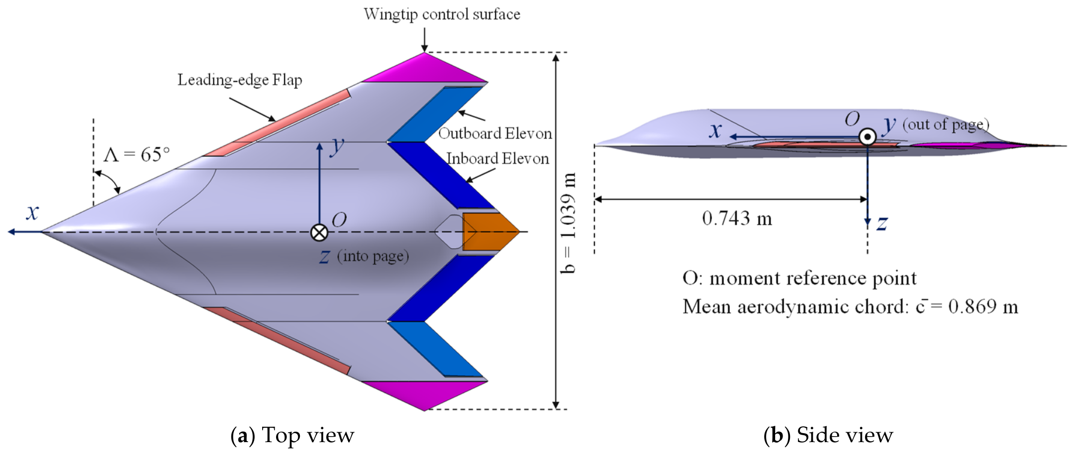
The aspect ratio is defined as the square of the wing span divided by the wing area, , and is a key parameter describing the planform slenderness of a wing. Low-aspect-ratio wings include configurations with AR below approximately 3, with typical examples including delta wings, missile wings with flying-wing layouts, some micro-air-vehicle wings and advanced military or civil aircraft. Although low-aspect-ratio wings have lower lift-to-drag efficiency than high-aspect-ratio wings, which rely mainly on attached flow for lift generation, they offer high structural stiffness, large internal volume, low supersonic wave drag, low rolling inertia and rapid maneuvre response. They are therefore widely used in fighters, missiles, unmanned combat aircraft and highly maneuverable micro air vehicles. The present work uses a scaled low-aspect-ratio flying-wing standard model with an aspect ratio of 1.54 and a leading-edge sweep angle of 65 deg, representing a typical blended flying-wing configuration. Figure 1 shows the original model geometry. Table 1 gives the reported reference dimensions.
Figure 1.
Schematic of the low-aspect-ratio baseline model.
Table 1.
Basic parameters of the low-aspect-ratio scaled model.
Low-aspect-ratio flying wings exhibit substantial aerodynamic curvature and separated-flow nonlinearity at high incidence [12,13]. This makes a broad angular database valuable, while also increasing the importance of local error and operating-region checks. The present static, control-increment and local-derivative tables provide complementary coefficient information over this angular domain. Their reconstruction supports subsequent model construction; validation of time-dependent hysteresis or aircraft trajectories requires the corresponding motion-response data.
2.2. Wind-Tunnel Test Procedure
2.2.1. Wind-Tunnel Facility and Support System
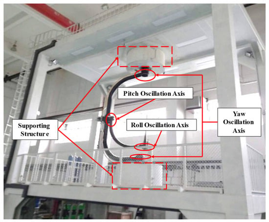
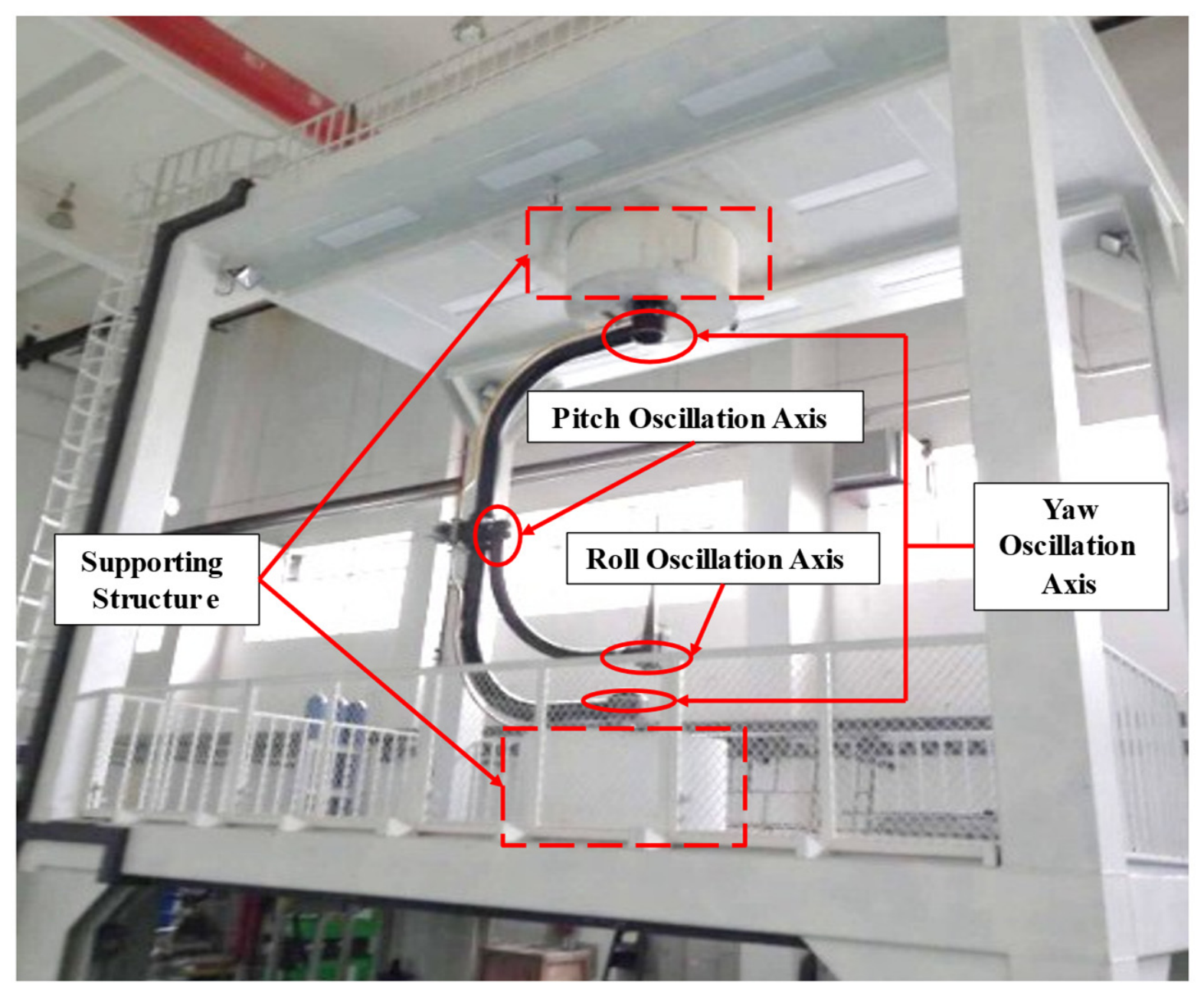
All wind-tunnel tests in this study were conducted in the FL-51 low-speed wind tunnel (AVIC Aerodynamics Research Institute, Harbin, China). The facility is a closed-circuit low-speed wind tunnel equipped with a six-component strain-gauge balance, a dynamic-pressure acquisition system, a three-degree-of-freedom static and dynamic support system, and a data-processing system. Figure 2 identifies the supporting structure and the pitch, roll and yaw oscillation axes in the supplied installation photograph.
Figure 2.
Wind-tunnel installation showing the supporting structure and the pitch, roll and yaw oscillation axes.
Because the low-aspect-ratio flying-wing configuration has a relatively flat aft body and lacks conventional horizontal and vertical tails, the installation of the force-measurement system presented particular challenges. A sting support was adopted as the primary support configuration, with a six-component strain-gauge balance installed inside the aft body. The model was rigidly connected to the front flange of the balance, while the sting was attached to its rear end and extended aft to the support system. To accommodate the balance, the aft-body geometry was locally enlarged during the support-system design. Under aerodynamic loading, elastic deformation of the balance and sting assembly can cause the actual model attitude to deviate from the prescribed setting. An elastic-angle correction was therefore applied during data reduction to compensate for this deviation and reduce the associated systematic errors in the aerodynamic measurements. This correction is particularly important in high-angle-of-attack regions, where aerodynamic coefficients may vary rapidly with incidence. No aerodynamic correction for sting-support interference was applied to the coefficient tables used in this study, and the magnitude of this effect was not quantified.
2.2.2. Test Conditions and Data Acquisition
The test model is a representative low-aspect-ratio flying-wing configuration with an aspect ratio of 1.54 and a leading-edge sweep angle of 65°. The aerodynamic database is parameterized by angle of attack, sideslip angle, and control-surface deflection. The angle-of-attack range covers the linear, post-stall, and high-incidence regimes to characterize nonlinear aerodynamic behavior over a broad operating envelope. The sideslip-angle range encompasses the principal operating conditions considered in the test program. Control surfaces, including ailerons, elevators, leading-edge flaps, drag rudders, and wingtip rudders, were independently deflected on the left and right sides, with deflection ranges and increments corresponding to the prescribed measurement sequences. Both static force measurements and forced-motion measurements were conducted to obtain the aerodynamic characteristics required for database construction, including static coefficients, control increments, and local aerodynamic derivatives.
After the wind tunnel was started and stabilized at the specified wind speed, the support mechanism gradually adjusted the model to the prescribed angle-of-attack sequence. At each discrete angle of attack, the model was held long enough for the balance signal to stabilize. The data-acquisition system then synchronously recorded the raw voltage outputs of the six-component balance. This process was repeated under combinations of sideslip angle and control-surface deflection. The acquisition system amplified and digitized each balance-channel voltage and stored the results on a computer, together with the operating condition, including angle of attack, sideslip angle, control-surface deflection and wind-tunnel environmental parameters.
The wind-tunnel tests were conducted at a nominal freestream velocity of 40 m/s using a six-component strain-gauge balance with a specified accuracy of 0.1% of full scale (F.S.). The mean aerodynamic chord of 0.869 m was adopted as the reference length for Reynolds-number characterization. Following experimental data reduction and the application of the available attitude corrections, the aerodynamic measurements were interpolated onto structured grids to establish the corresponding coefficient tables. These processed tables provide a consistent data source for model training, reconstruction evaluation, and hybrid database integration. The present study focuses on reconstructing these established aerodynamic coefficients and evaluating the relative performance of different reconstruction methods under identical reference-data conditions. The processed database does not contain the run-specific air properties needed to determine the Mach number and chord-based Reynolds number for each run. The available records are insufficient to quantify coefficient-level measurement uncertainty or the magnitude of any residual tunnel-wall or support-interference effects. Consequently, the reported reconstruction errors quantify agreement with the processed coefficient tables. Assessing absolute aerodynamic accuracy would require an experimental uncertainty budget and independent reference measurements.
The aerodynamic data used in this study are divided into three types, as summarized in Table 2: static basic characteristics, control increments and dynamic derivatives.
Table 2.
Classification of aerodynamic data in the database.
Static basic characteristics: and . Each input has two angular coordinates and each label has six dimensionless components. Stored fields cx, cy, cz, mx, my and mz correspond to these coefficients in the stated order.
Control increments: and , with three inputs and six outputs. The standard baseline is at the same flow conditions. Other surfaces remain at baseline positions, and . Left and right surface tables are retained and queried separately; no symmetry transformation replaces their data during fitting or online assembly.
Dynamic derivatives: each field takes and returns six components. Under the normalized-rate convention in the nomenclature, dyRoll stores , dyYaw stores , dyPit_dw stores , and dyPit_da stores . Within each field, cxw, cyw, czw, mxw, myw and mzw follow the order of . The derivatives and normalized rates are dimensionless; their products supply local first-order coefficient contributions.
2.2.3. Aerodynamic-Data Calculation
The body-axis system defined according to the British–American convention is used in this study:
The body-axis coordinate system has its origin at the moment reference point, located 0.743 m aft of the model nose. The positive x-, y- and z-directions are forward, toward the right wing and downward, respectively. The reference area, span and mean aerodynamic chord are 0.699 m2, 1.039 m and 0.869 m, respectively (Table 1).
The corresponding force and moment components are defined as follows:
Forces: is axial force, positive forward; is side force, positive to the right; and is normal force, positive downward. The corresponding dimensionless force coefficients are Cx, Cy and Cz.
Moments: L is the dimensional roll moment, positive for right-wing-down rotation. M is the pitch moment, positive nose-up. N is the yaw moment, positive nose-right. The corresponding dimensionless moment coefficients are Cℓ, Cm and Cn.
The six-dimensional balance loads are nondimensionalized using dynamic pressure, reference area and the appropriate moment reference length. This removes the chosen dimensional scaling; it does not remove dependence on Reynolds number, Mach number, transition state or configuration.
Here , where ρ is the air density and V is the freestream speed. The span normalizes rolling and yawing moments; the mean aerodynamic chord normalizes pitching moment. denotes reference area. The software fields mx, my and mz are coefficient labels corresponding to and .
3. Database Characteristics and Intelligent Construction Framework
All database modules use the supplied tables formed by interpolation of the wind-tunnel data. The database contains a two-input, six-output static table, twelve three-input, six-output single-surface increment tables, and four two-input, six-output local-derivative tables. Their input coordinates and coefficient ordering are defined in Section 2.2.2. This separation allows each table to use a representation suited to its sampling structure. The query interface forms the total coefficient vector by adding the static baseline, individual control increments, and local-derivative terms multiplied by their corresponding nondimensional rates. This first-order additive approximation neglects interactions between these contributions and flow-history effects.
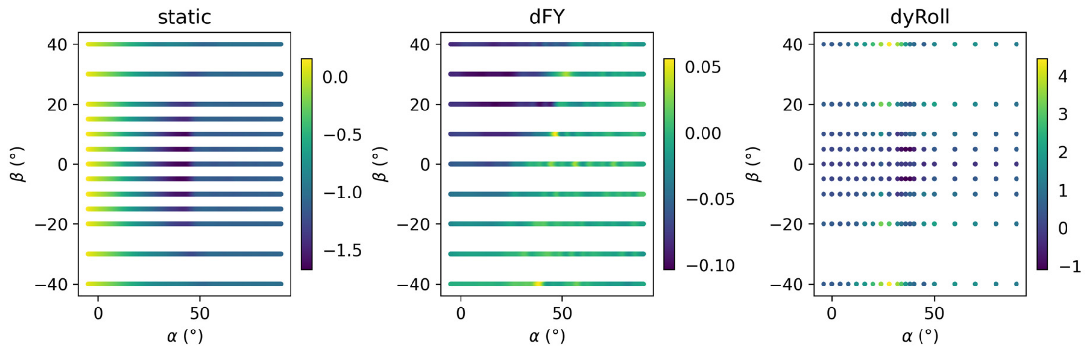
The three representative blocks contain 2483 static nodes (191 values 13 values), 8595 dFY nodes (191 9 5) and 180 roll-derivative nodes (20 9). The static and control domains span to and to ; the dFY deflection levels are and .
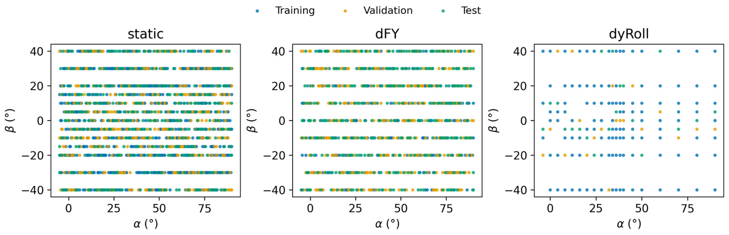
Figure 3 shows that the current data are not high-dimensional unstructured data, but low-dimensional structured tabular data. The static aerodynamic table covers a broad angle-of-attack range, with increased aerodynamic curvature and nonlinearity at high angles of attack. The control-effectiveness table has fewer sample points in the control-deflection dimension, which places higher requirements on local model generalization. The dynamic-derivative table has an even smaller sample size and is therefore suitable for small-sample surrogate modeling of the main trends.
Figure 3.
Tabulated angular-node distribution colored by or its corresponding increment/derivative channel; dFY shows .
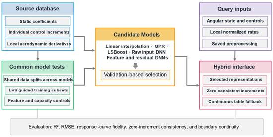
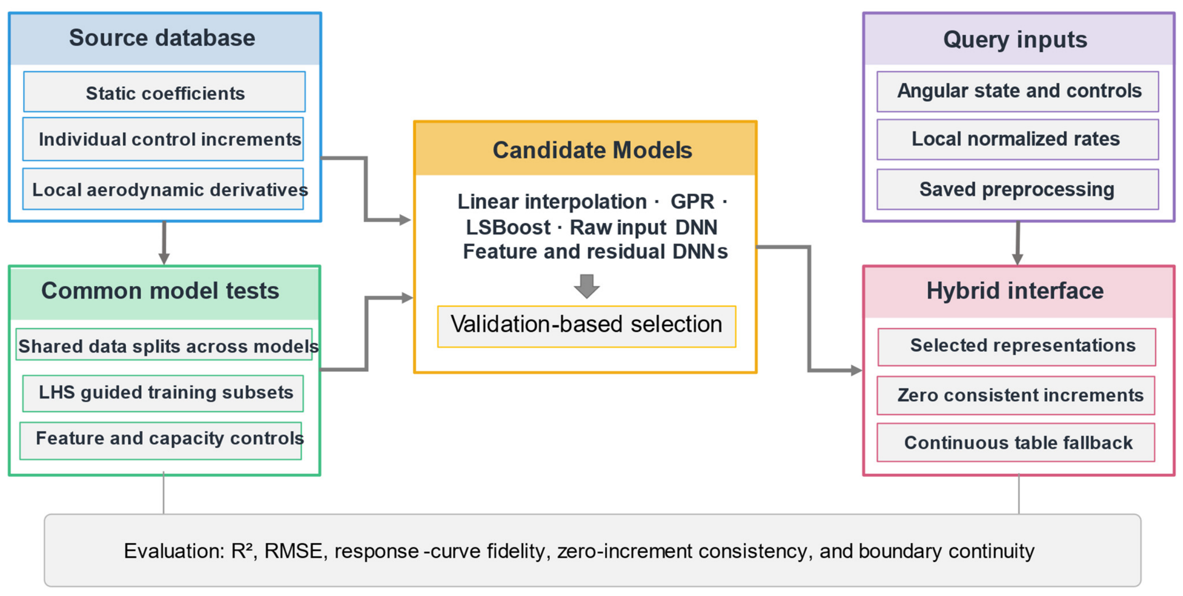
Figure 4 illustrates the overall framework connecting the source aerodynamic tables, model comparisons, and the hybrid coefficient-query interface. The static, control-increment, and local aerodynamic-derivative tables retain their distinct input coordinates and coefficient definitions. Within each comparison, candidate models share identical training, validation, and test partitions and the same training-data budget to ensure a fair evaluation. For random-node reconstruction, LHS-guided training subsets are selected from a separately established training pool, while blocked-condition tests retain structured grids to evaluate reconstruction under different missing-data scenarios. The candidate representations include linear interpolation, GPR, LSBoost, and DNN variants with raw inputs, engineered features, and residual learning. Independent validation guides representation selection for each module. The hybrid interface integrates the selected representations with the corresponding query inputs and saved preprocessing configurations, enforces zero control increments at neutral deflection, and ensures smooth transitions between surrogate predictions and retained table interpolation near domain boundaries. The resulting framework provides a unified evaluation and integration strategy addressing reconstruction accuracy, response-curve fidelity, physical consistency, and boundary continuity.
Figure 4.
Hybrid database construction and query workflow. Model comparisons using shared data splits support validation-based representation selection. Zero-deflection consistency and a smooth transition to retained table interpolation support coefficient integration.
4. Modeling Method
4.1. Sample Organisation and Representative Sampling
Training samples are formed by Cartesian ndgrid expansion, with as the fastest-varying coordinate when arrays are vectorized. Static and derivative inputs are (); control inputs are (). Unless stated otherwise, six scalar regressors share the same input rows and predict the six components independently. One-based row indices follow MATLAB R2025a (MathWorks, Natick, MA, USA) column-major ordering, with α varying fastest, followed by β and then δ where present.
The original random-node benchmark has two stages. First, within each α layer, the nodes are permuted using MATLAB’s Twister generator with seeds 41–45. The first max(1, floor(0.2 × layer size)) nodes enter the test set, the next equally sized group enters validation and the remaining nodes form the training pool. The validation and test counts are each 382 for static, 1719 for dFY and 20 for dyRoll. Second, the LHS mapping below selects training nodes only from the pool. Static budgets are 100, 400 and 800, dFY budgets are 120, 400 and 1200, and dyRoll budgets are 30, 80 and 120. Figure 5 shows the saved training, validation and test nodes for seed 41.
Figure 5.
Saved mutually exclusive training, validation and test nodes for seed 41; dFY displays the slice.
For the second stage, restart the generator at the same split seed and scale each training-pool coordinate to [0, 1] using its pool minimum and range. For a largest budget N, independently permute the integers 1 to N for each coordinate, subtract independent uniform draws on (0, 1), and divide by N [26]. In row order, map each design point to the nearest unused pool node by squared Euclidean distance, resolving ties by the first pool index. Smaller budgets take prefixes of that order. This rule applies to static, dFY and dyRoll in the original random-node benchmark. Mapping and truncation can change exact Latin-hypercube stratification. Blocked grids and the additional dyRoll partitions use their specified layer-based rules without LHS.
4.2. Machine Learning Models
The candidate families address different reconstruction needs. GPR supplies a smooth probabilistic response surface for low-dimensional data [21]. LSBoost combines local tree regressors to represent nonlinear responses [22]. Raw-input DNNs provide flexible feed-forward regression, while feature and residual variants test whether an alternative representation or a targeted correction improves the same task. Evaluating these families under common budgets provides the basis for module-specific selection.
The original scalar neural benchmarks use MATLAB fitrnet with ReLU, L-BFGS, an iteration limit of 420 and λ = 10−5 unless a sensitivity setting is stated. The raw-input and shallow feature networks use hidden widths [64, 32], while the deep variants use [128, 64, 32]. Each of the six scalar outputs uses the split seed plus 100 times its channel index (1–6). Neural-network and GPR predictors are standardized on the training nodes. Scalar labels are centered and divided by the training sample standard deviation, with unit scale used for constant labels. Predictions are returned to coefficient units. LSBoost uses 180 cycles, learning rate 0.05 and the default MATLAB regression-tree settings.
For each coefficient, GPR uses standardized raw inputs , a constant mean and an ARD squared-exponential kernel:
Exact marginal-likelihood fitting with the MATLAB default quasi-Newton optimizer estimates the length scales, signal scale and an output-specific noise parameter for each scalar regressor. Output centering and scaling use training-only statistics, and predictions are returned to coefficient units. Appendix A reports network sensitivity and component-level errors (Table A1, Table A2, Table A3, Table A4 and Table A5), predictive-interval coverage (Table A6) and fitted parameter ranges (Table A7).
For models using engineered angular features, the two-input feature map is
The corresponding three-input feature map is
where, , and the raw angles remain in degrees. Feature expansion precedes centering and scaling; the normalization statistics are fitted on training nodes and saved for use in validation and test prediction. The two maps contain nine and sixteen predictors, respectively. These engineered representations do not, by themselves, enforce the zero-deflection identity.
The original Res-Boost-DNN combines a feature-based LSBoost model with a residual network containing two hidden layers of 64 and 32 neurons. The network is trained to predict the residuals of the LSBoost model on the training data. To assess residual learning using predictions made on held-out training samples, we additionally evaluate a five-fold cross-fitting scheme. The outer training set is divided into five folds, and each fold receives residual targets from a base model trained on the other four folds. These out-of-fold residuals are used to train the residual network, after which the base model is refitted on the full outer training set. Neither validation nor test data are used to fit either component. We also evaluate the same residual-learning scheme with the raw-angle GPR benchmark as the base and report the GPR-only results for comparison. Although GPR provides a smooth base, adding a ReLU residual network does not ensure that the combined predictor is differentiable everywhere.
For each cross-fitted model, an independent validation set determines whether the residual correction is retained. The corrected model is selected only if it achieves a lower mean NRMSE than its corresponding base; otherwise, the base model is used alone. This selection is completed before test evaluation, so the reported test results assess the predictive benefit of the validation-selected correction.
4.3. Evaluation Method
All candidates within a benchmark use identical training coordinates and coefficient labels. For random-node tests, scattered linear interpolation is constructed in min–max-scaled coordinates, with nearest-neighbor continuation outside the training-node convex hull. For blocked-grid tests, the reference methods use multilinear interpolation or PCHIP along α with linear interpolation in the remaining coordinates. Beyond the retained grid, the original implementations use nearest-neighbor fallback or coordinate clipping, whereas learned regressors are queried at the original, potentially exterior, coordinates. Those boundary-policy comparisons describe practical continuation strategies, not a like-for-like assessment of extrapolation capability. Accordingly, the upper-α experiments also include an explicit last-interval linear-extrapolation baseline on the same retained grid, allowing learned predictions to be compared with a baseline that is likewise permitted to extend beyond the observed α range.
Mean NRMSE on the independent validation set is the deployment selection criterion. Control-increment candidates must also satisfy the zero-deflection identity. Training nodes determine the fitted models and preprocessing, and test-set NRMSE, RMSE and R2 describe performance on withheld nodes. Test rankings can differ from the validation ranking used for deployment.
In Equations (5) and (6), denotes the number of test nodes, and is the sample standard deviation of the training labels for output channel . The denominator of uses the test-set mean, whereas mean NRMSE averages the normalized errors over nonconstant output channels. Because RMSE and scale component errors differently, they may yield different model rankings. Reported variability is expressed as the sample standard deviation across data partitions or model seeds, as applicable; it does not quantify measurement uncertainty or variability across repeated wind-tunnel experiments.
Random-node tests assess reconstruction within the supplied table. Blocked-grid tests exclude an interior α gap or a complete β plane, and dFY additionally excludes both δ = ±10° planes. The upper-α test withholds the highest 20% of α layers. It compares direct learned predictions with both the original boundary-fallback baselines and an explicit extrapolating baseline. The latter extends the slope between the last two retained α layers, interpolates linearly on the remaining coordinates and uses only the common retained grid. All upper-α test nodes lie beyond the retained α range and inside the other grid intervals.
For each blocked test, the training grid contains at most 25 evenly indexed levels and seven levels, together with the retained levels where applicable. Training and validation coordinates are shared across models and remain fixed over five repetitions; only the model seeds change. Non-test nodes outside the retained training grid provide validation data. If no such nodes remain, one interior layer is reserved for validation. These blocked tests serve as retrospective diagnostics. Their test labels are excluded from automated feature and hyperparameter searches, and deployment choices are based on validation scores from the separate random-partition benchmarks.
5. Experimental Results and Aerodynamic Interpretation
5.1. Overall Model-Accuracy Comparison
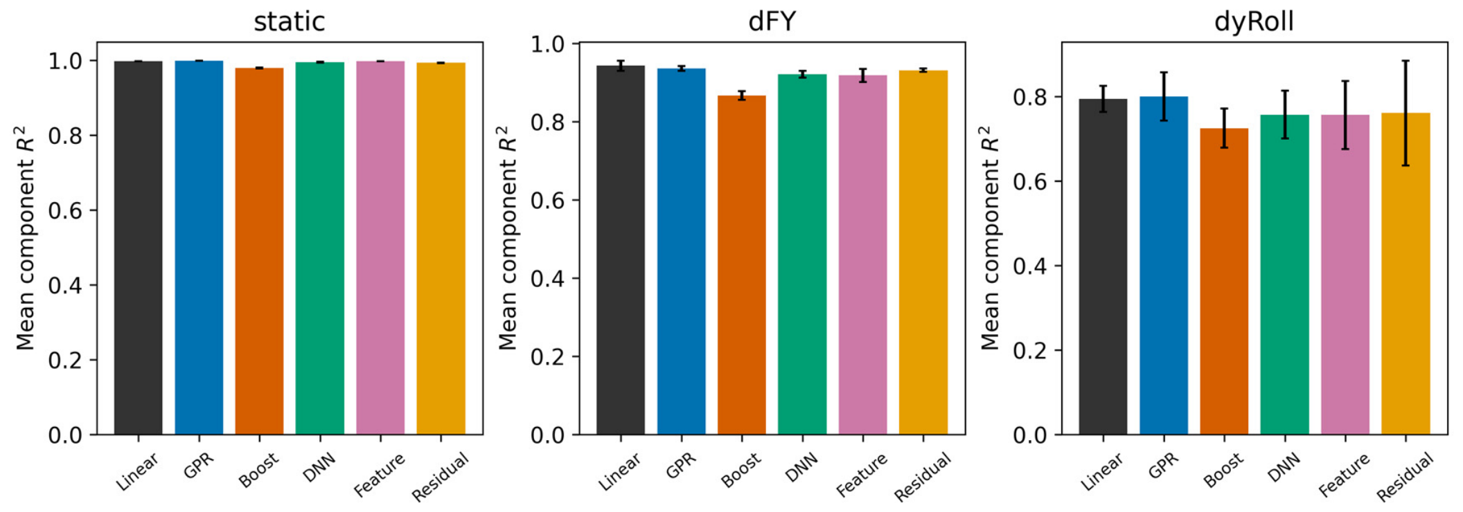
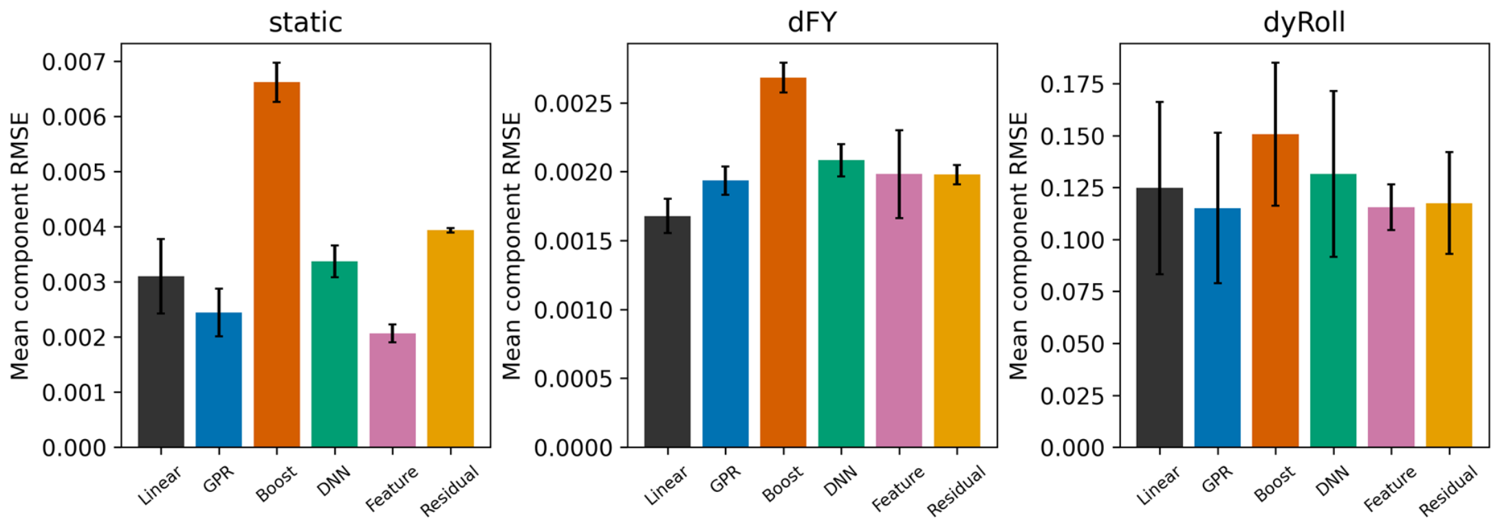
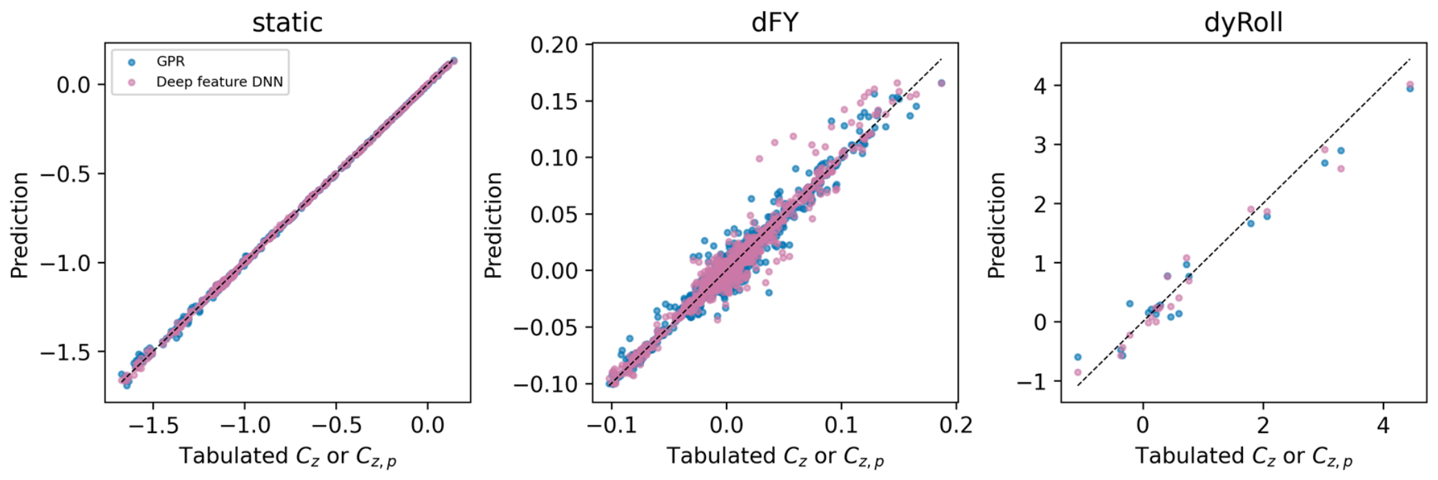
Table 3 summarizes the original same-node comparisons at the largest training budget for each module, with aggregate and component-level results shown in Figure 6, Figure 7, Figure 8, Figure 9 and Figure 10. The constrained and cross-fitted variants are evaluated separately in Section 5.6 to distinguish their effects from those of the original model formulations.
Table 3.
Overall prediction accuracy at the largest common budget. Mean NRMSE is reported as mean sample standard deviation over five partitions; and RMSE are partition means.
Figure 6.
Mean six-component at the largest budgets. Error bars denote sample standard deviations across five partitions.
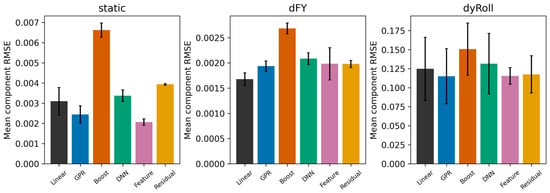
Figure 7.
Mean six-component RMSE at the largest budgets. Error bars denote sample standard deviations across five partitions.
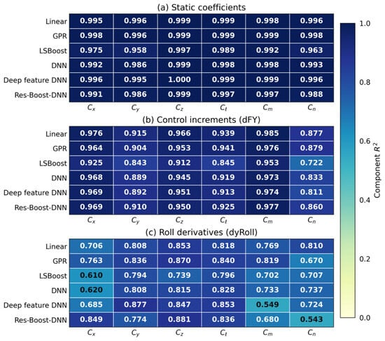
Figure 8.
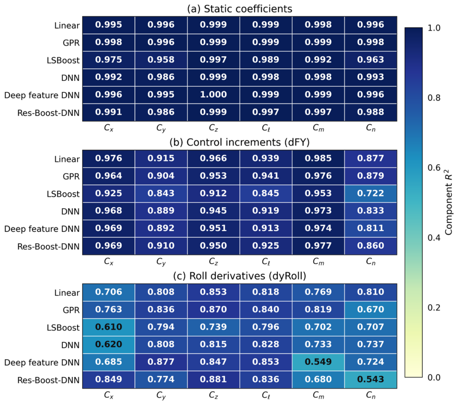
Component-wise of the principal models, averaged over five data partitions, for the static, control-increment and roll-derivative tables. All panels use a common color scale from 0 to 1, with numerical values shown to three decimal places. The moment channels correspond to the stored coefficients mx, my and mz.
Figure 9.
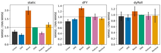
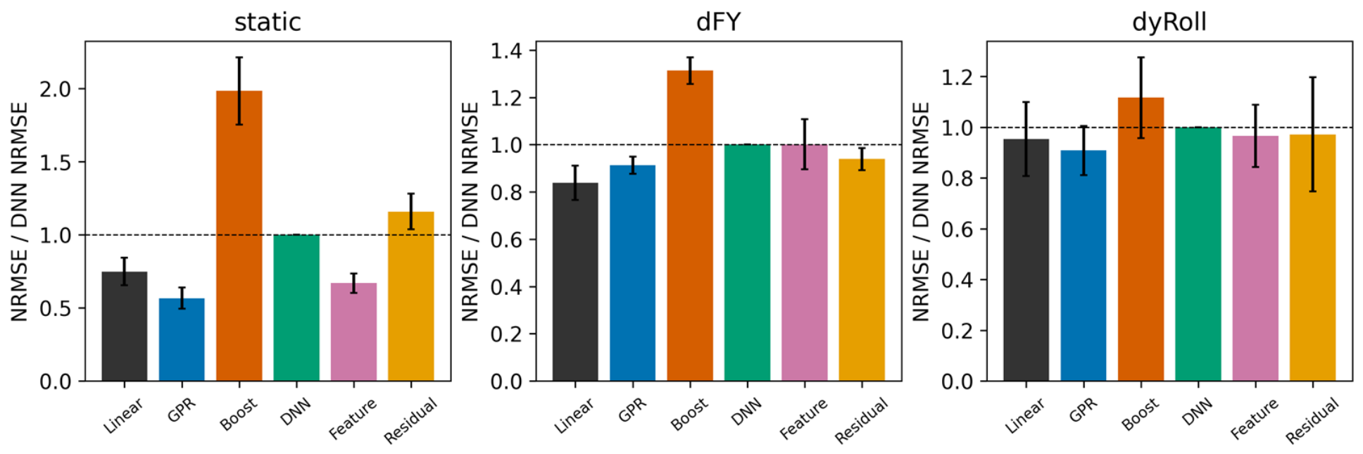
Paired NRMSE ratios relative to the standard DNN at identical partitions and budgets.
Figure 10.
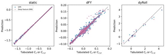
Normal-force-channel predictions at held-out nodes; seed 41 and largest budgets. The dashed diagonal in each panel indicates equality between predicted and tabulated values.
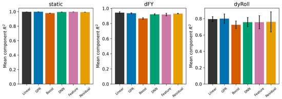
Figure 6 compares across modules. Static-table scores are consistently close to one, whereas derivative-table scores vary substantially across partitions, indicating greater sensitivity to the training-data selection.
Figure 7 reports RMSE on the original coefficient scale. Component-averaged RMSE therefore depends on the output scales and is unsuitable for direct comparison across modules. Its different weighting of component errors also explains why the highest- and lowest-RMSE models in Table 4 may differ.
Table 4.
Models with the best mean test scores and their aerodynamic interpretation. Deployment selection uses the separate validation set.
Figure 8 reveals differences among the six output channels that are obscured by aggregate scores. The corresponding component-wise NRMSEs in Table A3, Table A4 and Table A5 further identify channels with poor reconstruction accuracy, particularly among the local moment derivatives.
Figure 9 measures the relative error of each method against the standard DNN. Ratios below one indicate an improvement over this reference; comparisons with interpolation and other candidates require their corresponding absolute errors.
5.2. Static Aerodynamic Table Analysis
With 800 shared static training nodes, GPR reduces mean NRMSE from 0.0505 for linear interpolation to 0.0383, an improvement of 24.2%. The paired GPR-minus-interpolation difference is across five partitions, with GPR achieving lower error in every partition. GPR also yields the highest mean (0.9983), whereas the deep feature DNN achieves the lowest mean RMSE on the original coefficient scale (0.002062). These results demonstrate improved static-table reconstruction at a fixed sampling budget, while showing that representation selection depends on how component errors are weighted.
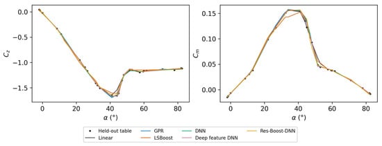
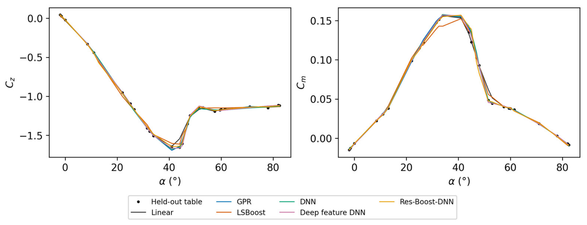
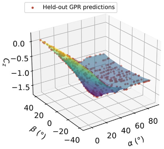
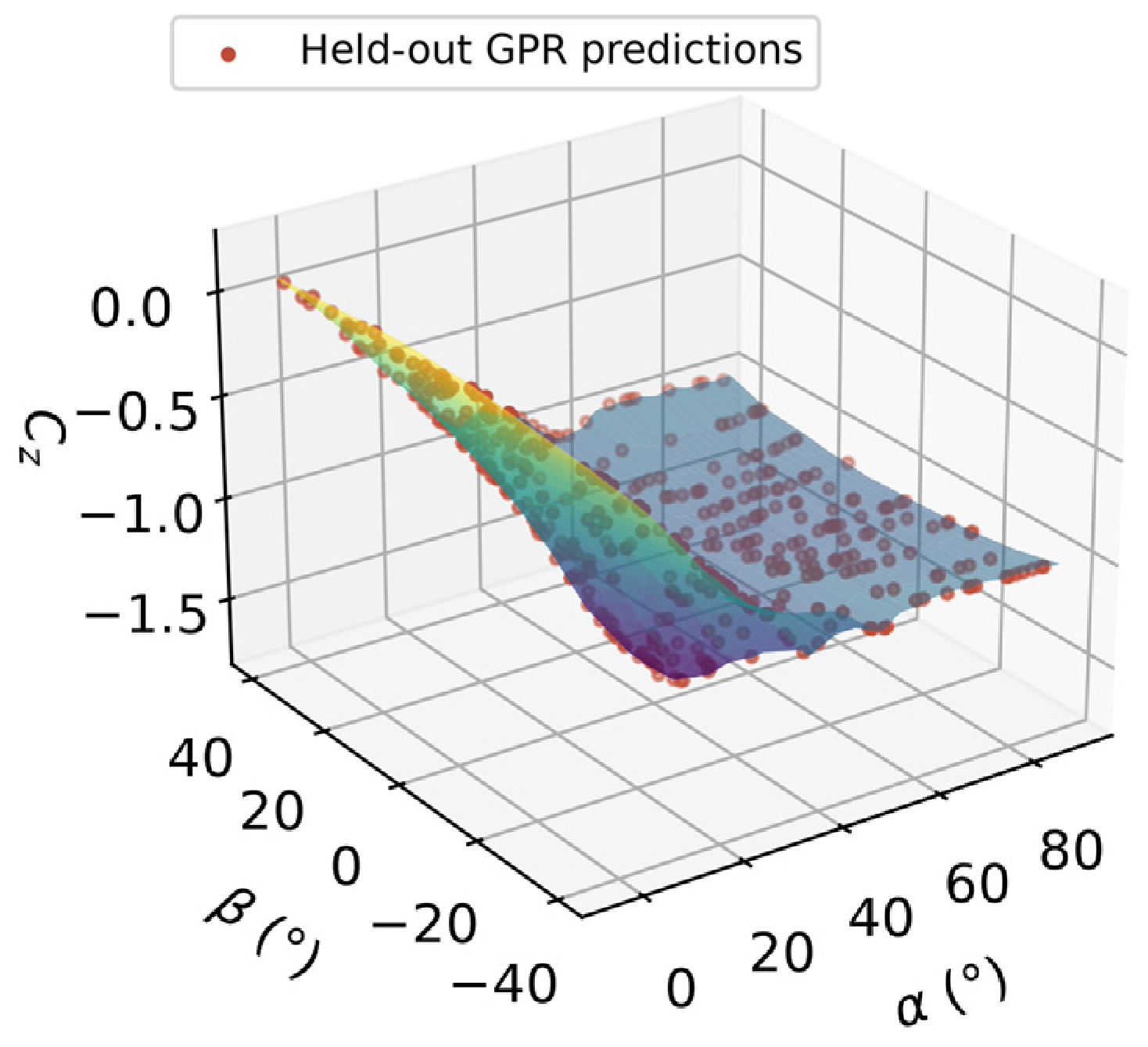
Figure 11 and Figure 12 complement the aggregate static-table metrics by showing the angular variation in individual coefficients. Figure 11 compares predictions at randomly withheld nodes on ; other nodes on the same plane may remain in training. Figure 12 presents the full static coefficient surface, providing context for the response curves and the variation that each representation seeks to reconstruct.
Figure 11.
Static and predictions at withheld test nodes; seed 41.
Figure 12.
Static table surface and GPR predictions at held-out nodes; and in degrees. Surface colors encode the tabulated coefficient value.
5.3. dFY Control-Increment Table Analysis
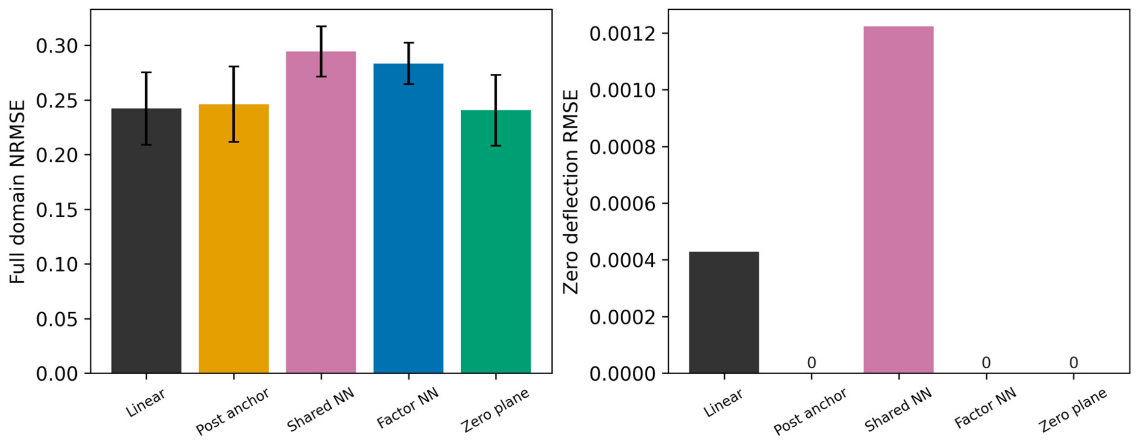
The dFY control-increment benchmark covers angle of attack, sideslip and control deflection, using 1200 shared training nodes and 1719 test nodes per partition. GPR achieves a mean of 0.9361 and mean RMSE of 0.001936, compared with 0.9211 and 0.002084 for the standard DNN. However, linear interpolation yields a lower mean NRMSE than GPR (0.2422 versus 0.2626). Thus, the static-table advantage of GPR does not extend uniformly to control increments, supporting the use of different representations within the hybrid database.
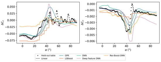
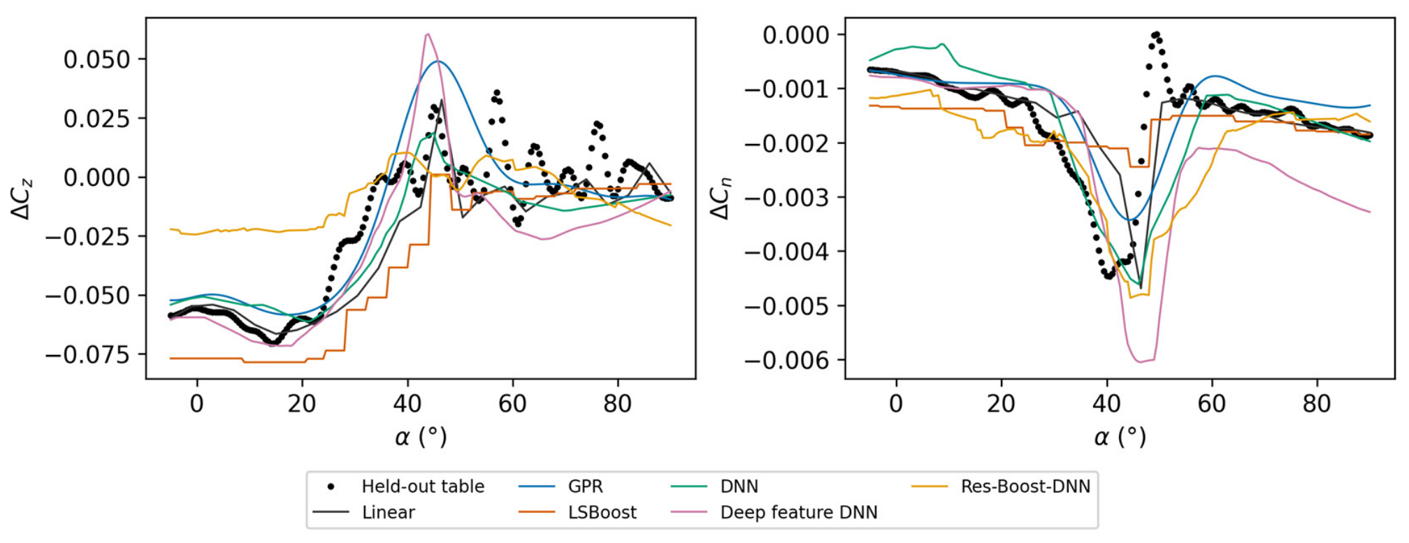
Figure 13 examines reconstruction across a missing operating plane: the entire plane is excluded from training, and predictions are evaluated along the curve. Table 5 reports the corresponding errors in and . These results complement the full-domain averages in Table 3 by assessing accuracy at a specific control condition. Their differing rankings show why database selection should consider both aggregate error and response fidelity at relevant operating conditions.
Figure 13.
dFY increments and at , with the entire plane excluded from training. Results use seed 41.
Table 5.
dFY held-out-curve error statistics for the selected and components ().
The control-effectiveness surface contains combinations of sideslip angle, angle of attack and control deflection, whereas a response curve represents one operating-condition slice. For a low-aspect-ratio flying wing, both descriptions are relevant to evaluating changes in normal force and control moments. A useful control-increment module should capture global trends and maintain acceptable errors at important control conditions. Separate validation-based selection allows the database to retain interpolation or a learned representation according to the available evidence.
At zero deflection, the supplied control increments are exactly zero. Nevertheless, sparse scattered interpolation can produce nonzero predictions when zero-deflection nodes are omitted from training. Preserving this identity therefore requires an explicit constraint in the query representation. Section 5.6.3 compares zero-anchored versions of the primary models over the same full test domain, quantifying how enforcement affects reconstruction accuracy and model ranking. This extends the comparison beyond predictive accuracy to the consistency required when integrating individual control increments into the hybrid database.
5.4. Roll Dynamic-Derivative Table Analysis
The 180-node roll-derivative table provides a small-data test of the candidate representations. Across five partitions with 120 training nodes and 20 test nodes each, mean NRMSE is for linear interpolation, for GPR and for the deep feature DNN. The paired GPR-minus-interpolation difference is . Although both learned models achieve slightly lower mean errors, the variation across partitions limits the evidence for a stable ranking. These results highlight the importance of sampling sensitivity when selecting representations for sparsely populated derivative tables.
The roll-derivative coefficients describe local sensitivities to the nondimensional roll rate and supply the corresponding rate-dependent contribution to the first-order aerodynamic model. Their reconstruction therefore complements the static and control-increment modules within the hybrid database. The present comparison assesses the accuracy of these local coefficient fields; resolving hysteresis, vortex evolution and phase lag additionally requires time-resolved motion and load measurements.
5.5. Feature Ablation and Blocked-Condition Validation
Table 6 separates feature expansion, network depth and the residual stage using identical partitions and training budgets: 400 nodes for static and dFY, and 80 for dyRoll. At 400 static nodes, the shallow feature DNN reduces mean normalized RMSE from 0.0978 to 0.0820, a 16.2% reduction; increasing its depth gives 0.0751. The corresponding improvement is not observed for dFY. Relative to feature-based LSBoost alone, residual correction lowers the mean error for static and dyRoll but slightly raises it for dFY. These comparisons support module-specific assessment of architectural choices.
Table 6.
Feature, depth and residual-stage ablations: mean NRMSE sample standard deviation over five partitions.
The blocked-condition results in Table 7 underscore why a reconstruction algorithm cannot be ranked independently of the withheld region and the interpolation policy. For an interior static α gap, GPR reduces mean NRMSE from 0.7880 for multilinear interpolation to 0.5536, while the deep feature DNN yields 0.4925. For static upper-α queries, the deep feature DNN (0.1361) outperforms the original boundary-fallback interpolants (0.2480 and 0.1833), but explicit linear extrapolation from the same retained grid achieves a still lower 0.0876. The latter result prevents attributing an inherent extrapolation advantage to the learned model. In the dFY and dyRoll upper-α tests, the corresponding linear-extrapolation scores are 0.6877 and 6.5835, illustrating that extending a local slope is not universally effective. The evidence therefore supports scenario-dependent representation choice, not a uniform superiority claim for learning or interpolation.
Table 7.
Mean NRMSE for blocked conditions over five model seeds. Parentheses give training-node counts. The original interpolation baselines use boundary fallback for exterior points.
5.6. Validation of Reconstruction and Database Consistency
The following experiments examine how representation choices affect reconstruction accuracy and consistency during database assembly. They assess network capacity, engineered features, residual correction and zero-deflection constraints using matched data partitions and independent validation sets. Together, these comparisons establish when additional model structure benefits a database module. Appendix A shows learning curves, feature-group ablations, derivative reconstruction diagnostics, regional errors and zero-consistency comparisons (Figure A1, Figure A2, Figure A3, Figure A4 and Figure A5).
5.6.1. Network Capacity, Features and Activation
Table A1 examines network width, regularization and parameter-matched raw-input controls. The comparisons include [32, 16] and [64, 32] networks and regularization strengths of . For two inputs, the nine-feature [64, 32] network contains 2753 parameters per scalar output, compared with 2760 for the raw-input [77, 32] control. For three inputs, the corresponding sixteen-feature network contains 3201 parameters, compared with 3197 for the raw-input [87, 32] control. These comparisons assess whether feature expansion offers benefits beyond a comparable increase in parameter count.
The original 420-iteration entries in Table A1 report held-out test NRMSE. To assess convergence, we compare ReLU with Swish/SiLU, defined as t/(1 + exp(−t)). Both activations were refitted using SciPy 1.15.3 L-BFGS-B without parameter bounds on the original partitions. Each paired [64, 32] network shares standardized data, Glorot-uniform weights and zero biases. The objective is mean squared error plus λ/2 times the sum of squared weights, with λ = 10−5. Every fit met the same objective-reduction stopping criterion (ftol = 10−9). ReLU used 629–10,286 iterations and Swish used 6589–38,979. For static data, final training NRMSE is 0.0133 for ReLU and 0.0240 for Swish/SiLU. At iteration 420 of the matched reruns, static test NRMSE is 0.1003 and 0.1387, respectively. At convergence, these test errors are 0.0861 and 0.0925. Longer training narrows the static test-error gap. For dFY and dyRoll, Swish achieves lower mean training NRMSE, while ReLU achieves lower mean test NRMSE in the extended comparison.
Table A2 and Figure A2 assess the contributions of trigonometric, squared and interaction features through matched-depth ablation. At 400 static training nodes, feature expansion reduces mean NRMSE from 0.0978 to 0.0820, a 16.2% improvement. Removing squared terms gives 0.0808, with little difference relative to partition variability. For dFY, however, the complete feature map increases error from 0.4257 to 0.4784. Feature expansion therefore provides a module-dependent regression benefit; these tests do not establish that individual feature groups encode an aerodynamic mechanism.
5.6.2. Residual Cross-Fitting and Base-Model Choice
Table 8 compares residual correction for LSBoost and GPR bases using residual targets generated by five-fold cross-fitting. Independent validation determines whether each correction is retained, and its performance is then evaluated on the outer test set. This separates the ability to fit training residuals from the ability to improve predictions on unseen nodes.
Table 8.
Cross-fitted residual-learning performance on independent test nodes, reported as mean NRMSE sample standard deviation. Training budgets are 400, 400 and 80 nodes for static, dFY and dyRoll, respectively. Bracketed counts indicate partitions in which validation selects the residual correction.
For the LSBoost base, validation retains the correction in all five static partitions, reducing test NRMSE from 0.1575 to 0.1496. It rejects the correction in every dFY and dyRoll partition. For the GPR base, validation retains the uncorrected model in all static and dFY partitions. The raw-angle GPR also remains more accurate than the corrected LSBoost model on static data. These results support selective residual correction when it improves a candidate representation.
Smoothness remains a separate consideration. A continuous residual network generally cannot remove discontinuities inherited from a tree base, while a ReLU correction can introduce derivative discontinuities into a smooth GPR predictor. Residual correction should therefore be assessed against both reconstruction accuracy and the continuity requirements of the intended query.
5.6.3. Zero-Consistent Control Increments
Zero-deflection consistency is first enforced by subtracting each model’s predicted neutral-control increment:
This construction guarantees without additional labels or an odd-symmetry assumption. It is applied to all primary models, including sparse scattered interpolation.
Two further designs embed the identity directly in the representation. The first uses a shared six-output network,
where is expressed in degrees. At nonzero deflections, the network is fitted to with weights , preserving a loss proportional to coefficient squared error. At zero deflection, the identity holds analytically. Matched constrained and unconstrained networks use sixteen predictors, training-only input standardization and output-standard-deviation scaling without centering. Both use ReLU and 420 L-BFGS iterations. Each family is selected independently from the same four validation candidates, combining widths [32, 16] or [64, 32] with or . The architectures contain 1174 or 3366 parameters per six-output network; the multiplicative constraint adds no parameters.
The second design completes the prescribed zero-deflection plane using the exact increment identity. Separate positive- and negative-deflection scattered interpolants meet at this plane, without assuming odd symmetry. Coordinate normalization matches the original interpolation baseline. After duplicate removal, the construction adds 1518–1520 analytical zero constraints while retaining the same 1200 source-table training nodes. These anchors encode known zero values rather than additional measurements or access to withheld nonzero labels.
Table 9 and Figure A5 show that the method of enforcing the identity affects full-domain accuracy. Post hoc subtraction slightly increases interpolation NRMSE from 0.2422 to 0.2460. By contrast, the factorized network reduces its matched unconstrained error from to , a 3.7% improvement, with lower error in four of five partitions.
Table 9.
Zero-consistency comparisons using 1200 dFY training nodes across five partitions. The first six rows apply post hoc anchoring to the primary models. The remaining rows evaluate matched neural formulations and the zero-plane interpolant.
The zero-plane interpolant incorporates the exact zero-deflection identity into the interpolation process by introducing a neutral-control reference plane that connects the positive- and negative-deflection branches. This construction preserves the baseline aerodynamic coefficients at zero deflection while retaining the ability of interpolation to capture variations across the control-deflection domain. As shown in the five dFY partitions, the proposed interpolant consistently achieves lower reconstruction errors than conventional interpolation, reducing the mean test NRMSE from 0.2422 to 0.2406. Although the improvement in overall accuracy is relatively modest, its consistency across different partitions, together with the exact satisfaction of the neutral-control condition, makes the zero-plane interpolant a suitable representation for control-increment reconstruction. Based on independent validation, this constraint-preserving interpolation strategy is therefore adopted for the dFY module in the hybrid query interface.
5.6.4. Derivative Reconstruction and Layer Exclusion
The 180-node dyRoll table is evaluated on 20 additional partitions (Twister seeds 101–120). Within each α layer, a random permutation assigns two β nodes to testing, one to validation and six to training, giving 40, 20 and 120 nodes, respectively. In the separate layer-exclusion test, each of the 20 complete α layers serves as the test set once. The lowest and highest remaining layers serve as validation, leaving 153 training and nine test nodes. All candidates share those nodes. For the interpolation baseline, exterior queries use nearest-neighbor continuation from the training points. Learned models receive the original coordinates. Table 10 summarizes the random-node and layer-exclusion results.
Table 10.
Additional dyRoll reconstruction diagnostics. Layer-exclusion scores are averaged equally over 20 withheld layers. Wins indicate lower paired NRMSE than linear interpolation.
On the 20 additional random-node partitions, GPR reduces mean NRMSE by 7.8% and gives the lower paired error in 19 cases. These partitions repeatedly sample the same 180-node table. For complete layer exclusion, the linear baseline gives 0.3125 versus 0.3565 for GPR. Across the 16 interior layers, the corresponding means are 0.3609 and 0.3794. Across the four exterior layers, they are 0.1192 and 0.2647, comparing nearest-neighbor continuation with direct GPR prediction. These different conditions and the observed variation across splits limit model rankings to the tested table and validation design.
5.6.5. Predictive Uncertainty and Control-Relevant Diagnostics
GPR uncertainty is assessed using the empirical coverage of nominal 95% Gaussian observation-prediction intervals on held-out nodes. Averaged across partitions, component-wise coverage ranges from 93.5 to 95.0% for static data, 91.5 to 94.6% for dFY and 93.0 to 100.0% for dyRoll (Table A6). These results assess predictive calibration within the supplied tables; they do not quantify wind-tunnel measurement uncertainty or establish reliability under untested conditions. The intervals are used for calibration assessment rather than adaptive sampling.
Table A3, Table A4 and Table A5 report errors for all six output components. Figure A4 separates four ranges. These diagnostics reveal local discrepancies that aggregate scores can obscure. Table A8 additionally compares finite-difference slopes of with respect to and right-elevator deflection against full-table lookup. Evaluations use and , with a differencing step of . These checks assess how reconstruction errors affect local coefficient sensitivities relevant to subsequent trim and stability analyses. Table A9 identifies the largest normalized component errors.
5.7. Engineering Value and Applicability
The comparative results highlight the importance of adapting reconstruction strategies to the characteristics of individual aerodynamic data modules. While GPR and neural networks improve static-coefficient reconstruction under selected sparse-data conditions, the zero-plane interpolant provides a reliable solution for control-increment reconstruction by preserving the neutral-control identity. For the smaller dynamic-derivative table, the relative performance of learning-based methods and interpolation varies with the distribution of available samples. These findings demonstrate that reconstruction accuracy alone is insufficient to determine the most appropriate representation. By combining module-specific model selection with physical consistency constraints and continuous boundary transitions, the proposed hybrid framework exploits the complementary strengths of different reconstruction methods and enables their integration into a unified aerodynamic coefficient-query interface.
The framework provides a practical approach to improving the utilization of existing wind-tunnel aerodynamic databases without requiring additional experimental samples. Its current application focuses on reconstructing processed aerodynamic coefficient tables within a first-order additive assembly, where control-surface interactions and flow-history effects are not explicitly represented. Further investigations incorporating independent aerodynamic measurements and more comprehensive unsteady models would extend its applicability to broader flight-dynamics and control applications.
6. Constraint-Preserving Modular Query Interface
The hybrid query interface selects representations by independent validation mean NRMSE, with zero-deflection consistency as a requirement for control-increment candidates. The saved seed-41 configuration contains the deep feature DNN for static coefficients, the zero-plane interpolant for dFY and retained table lookup for dyRoll and the other modules. It records the selected representation, the applicable coordinate bounds and preprocessing constants for each fitted module.
Each selected model is evaluated within its saved coordinate bounds, with retained table lookup used outside those bounds. Within the outermost 5% of each coordinate range, the module output is blended as
where and . For each coordinate, is the distance to the nearer boundary divided by 5% of that coordinate’s range, clipped to [0, 1]. The blending weight and its first derivative vanish at the boundary. The model correction therefore approaches zero continuously, preventing representation-switching jumps while retaining the original lookup interpolation structure.
The total coefficient vector is assembled from the static contribution, individual control increments and local rate-dependent terms:
At neutral controls and zero normalized rates, the additive terms vanish and the interface returns the static coefficient vector. The assembly is first order in the local rate contributions and assumes additive individual control increments. Coupled-control, control–rate and flow-history effects would require time-resolved or jointly excited data and separate aerodynamic validation.
A prescribed 101-state query sequence tests the software interface and compares the outputs before and after reloading the saved configuration. Boundary tests cover every face of the static and dFY coordinate boxes. These checks verify numerical behavior. The withheld-node comparisons in Section 5 assess reconstruction of the source coefficients.
For both the static and dFY modules, the maximum difference from retained table lookup is zero at the tested boundary and exterior points, confirming correct fallback implementation. Paired queries across the boundaries yield a maximum coefficient difference of at a normalized separation of . This finite-distance check complements the blending construction, whose correction vanishes continuously at the boundary.
A separate 191-point sweep from to at evaluates neutral-control assembly. With all twelve controls at zero deflection and all normalized rates set to zero, the assembled output matches the static-only interface exactly. This confirms that module assembly introduces no spurious incremental contribution. Relative to full static-table lookup, the six RMSEs along this neutral-control sweep are 0.001172, 0.001065, 0.010388, 0.000619, 0.001526 and 0.000331, in the order . These differences quantify the remaining static reconstruction error separately from the verified zero-increment and assembly identities.
7. Conclusions
This study proposed a constraint-preserving hybrid reconstruction framework for constructing an intelligent aerodynamic database from heterogeneous static, control-increment, and local aerodynamic-derivative data. By integrating comparative reconstruction analysis, physical consistency constraints, and validation-based module selection, the proposed framework combines the complementary strengths of learning-based methods and conventional interpolation while ensuring consistent aerodynamic coefficient queries. The main findings are summarized as follows.
- (1)
- For static aerodynamic reconstruction, GPR demonstrated strong performance under sparse random-node sampling. With 800 training nodes, the mean NRMSE decreased from 0.0505 for linear interpolation to 0.0383, corresponding to a 24.2% improvement. The deep feature DNN achieved the lowest mean RMSE on the original coefficient scale. Under excluded-condition tests, reconstruction performance varied with the missing region and extrapolation strategy, highlighting the importance of scenario-specific model evaluation.
- (2)
- Feature engineering and network configuration significantly influenced reconstruction accuracy. With 400 static training nodes, engineered angular features reduced the matched-depth DNN test NRMSE from 0.0978 to 0.0820, whereas raw inputs remained more effective for the dFY control-increment table. Extended optimization further narrowed the performance difference between ReLU and Swish/SiLU, demonstrating the importance of sufficient convergence when evaluating neural-network configurations.
- (3)
- Incorporating physical constraints improved the consistency of control-increment reconstruction. The factorized network preserved the zero-deflection identity and outperformed its unconstrained counterpart. The proposed zero-plane interpolant further reduced the mean dFY test NRMSE from 0.2422 to 0.2406 while ensuring exact neutral-control consistency. Its favorable validation performance supported its selection for the hybrid database.
- (4)
- Dynamic-derivative reconstruction exhibited a strong dependence on sample distribution. For the 180-node dyRoll table, GPR reduced mean NRMSE by 7.8% across 20 additional random-node partitions and achieved lower errors in 19 cases. However, interpolation performed better when complete angle-of-attack layers were excluded, demonstrating the importance of matching reconstruction methods to the available data structure and operating-condition coverage.
- (5)
- The hybrid aerodynamic database integrated independently selected reconstruction modules with continuous transitions to retained table interpolation. Boundary, neutral-control, and save/reload tests confirmed the numerical consistency of the resulting coefficient-query interface. By combining data-driven reconstruction with exact coefficient constraints and selective interpolation, the framework provides a practical approach to improving the utilization of existing aerodynamic databases for subsequent simulation and model development.
The present framework focuses on reconstruction and consistent integration of existing aerodynamic coefficient tables. Future work will extend the approach to coupled-control effects and unsteady aerodynamic modeling, supported by additional aerodynamic validation under broader operating conditions.
Author Contributions
Conceptualization, J.W. and Y.L.; methodology, J.W.; software, J.W.; validation, J.L., C.W., Y.Y., M.H., C.B. and Y.W.; formal analysis, J.W. and Y.L.; investigation, J.L., C.W., Y.Y., M.H., C.B. and Y.W.; resources, C.B. and Y.W.; data curation, J.L., C.W., Y.Y., M.H., C.B. and Y.W.; writing—original draft preparation, J.W.; writing—review and editing, J.L., C.W., Y.Y., Y.L., M.H., C.B. and Y.W.; visualization, J.W.; supervision, Y.L.; project administration, Y.L. All authors have read and agreed to the published version of the manuscript.
Funding
This research was funded in part by the National Natural Science Foundation of China, grant number 12272104; in part by the National Natural Science Foundation of China, grant number U22B2013; in part by the Key Research and Development Program of Heilongjiang Province, grant number 2025ZX01A03; and in part by the Joint Fund of the National Natural Science Foundation of China, grant number U25B2090 (Project title: “Design of Continuous Smooth Morphing Trailing Edge and Aerodynamic-Structural Coupling Mechanism for Low-Aspect-Ratio Tailless Flying Wing Aircraft”).
Data Availability Statement
The article provides the sampling algorithm, indexing convention, preprocessing, model settings and deployment configuration. Requests for the source coefficient tables, exact split indices, implementation code and saved model configurations may be directed to the corresponding author. Release is subject to approval by the data holders.
Conflicts of Interest
The authors declare no conflicts of interest.
Nomenclature
Symbols and conventions used throughout this manuscript.
| Symbol | Meaning and Units |
| Angle of attack, sideslip and control deflection; degrees in table inputs | |
| Body-axis forces (N) and roll, pitch, yaw moments (N m) | |
| Dimensionless force and moment coefficient vector | |
| Freestream dynamic pressure (Pa), speed (m/s) and density (kg/m3) | |
| Reference area (m2), span (m) and mean aerodynamic chord (m) | |
| Body angular rates and angle-of-attack rate; rad/s before normalization | |
| Six-component derivatives of with respect to the corresponding normalized rates | |
| Root-mean-square error, training-standard-deviation-normalized RMSE and coefficient of determination | |
| Static coefficient vector, control-increment vector and deflection of surface i. | |
| Number of nodes and sample or coordinate/component indices in the sampling and error definitions. | |
| Neutral-anchored regression function, factorized network and its trainable parameters. |
Appendix A. Additional Numerical Evidence
All appendix results are derived from saved benchmark outputs and the additional analyses described in Section 5.6. Reported standard deviations summarize variability across the specified data partitions or excluded layers.
Table A1.
Network architecture, regularization and activation sensitivity for 400 static, 400 dFY and 80 dyRoll training nodes. Values are mean NRMSE ± sample standard deviation across five shared partitions. The original 420-iteration rows report test NRMSE. The extended activation comparison reports both training and test NRMSE.
Table A2.
Individual feature-group removal at [64, 32] networks and the same intermediate budgets.
Figure A1.
All three training budgets for each module, using the original five partitions. Error bars are sample standard deviations.
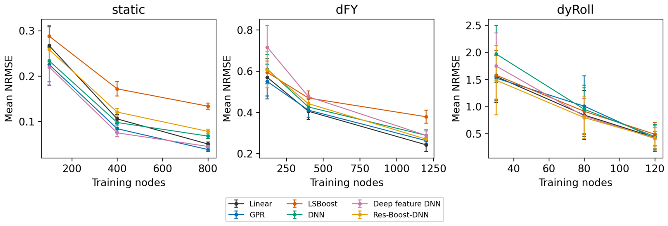
Figure A2.
Feature-group ablation at fixed network depth and matched training budgets. Error bars denote the standard deviation over five common partitions.
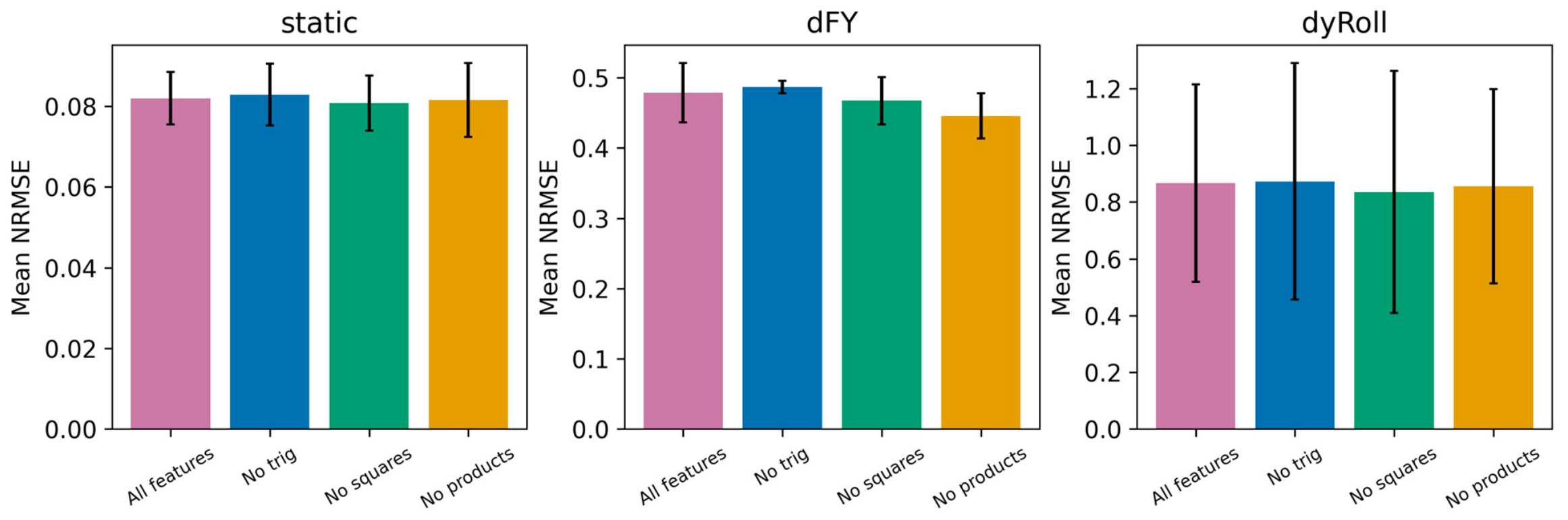
Table A3.
Component-wise NRMSE for static coefficients using 800 training nodes, averaged over five partitions.
Table A4.
Component-wise NRMSE for dFY control increments using 1200 training nodes, averaged over five partitions.
Table A5.
dyRoll component NRMSE at the largest common budget; five-partition means. Moment channels correspond to stored mx,my,mz.
Figure A3.
Additional dyRoll random-partition scores and leave-one--layer-out results. Each point is a partition or a complete excluded layer.
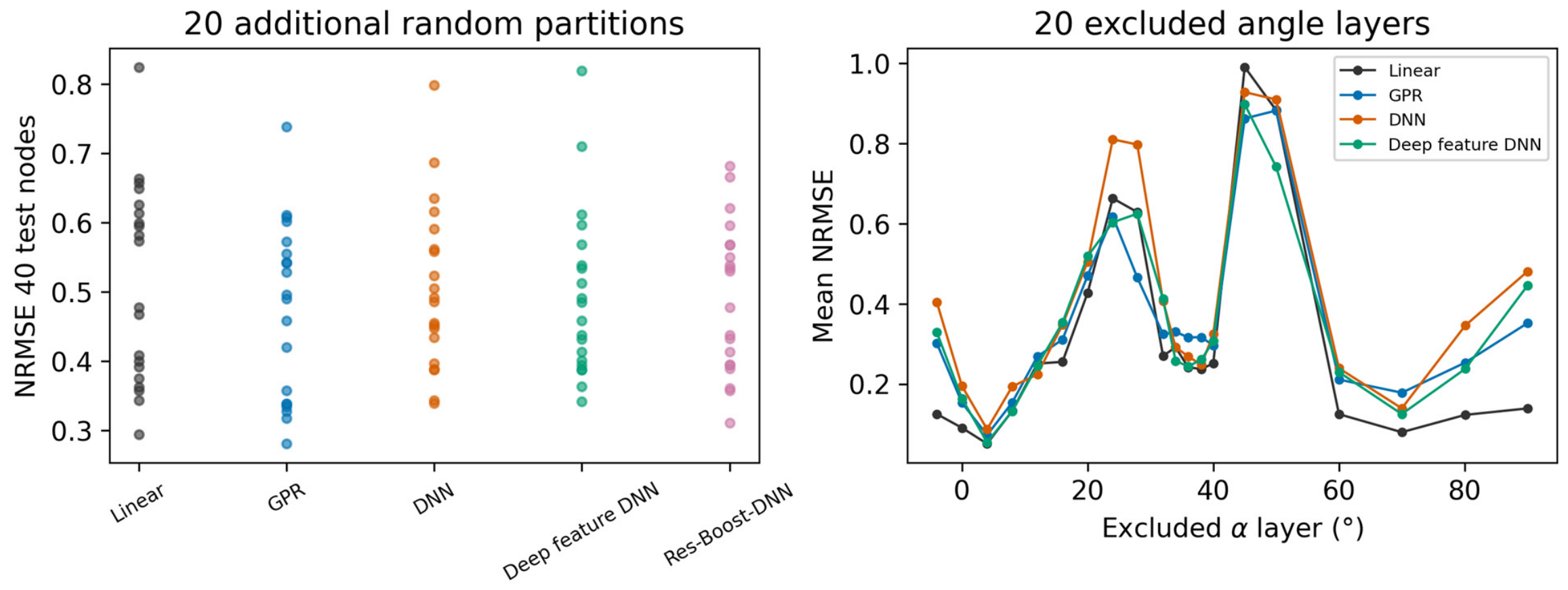
Table A6.
Empirical coverage of nominal 95% GPR prediction intervals on held-out test nodes, reported by output component and averaged over five partitions.
Table A7.
Fitted GPR hyperparameter ranges across six outputs and five partitions. Length scales refer to standardized inputs, signal scales to standardized outputs, and noise standard deviations to the original output scale.
Figure A4.
Regional mean NRMSE at the largest budgets. Each row is an α interval; intervals contain different numbers of test nodes. Darker shades indicate higher mean NRMSE within each panel, which uses its own color scale.
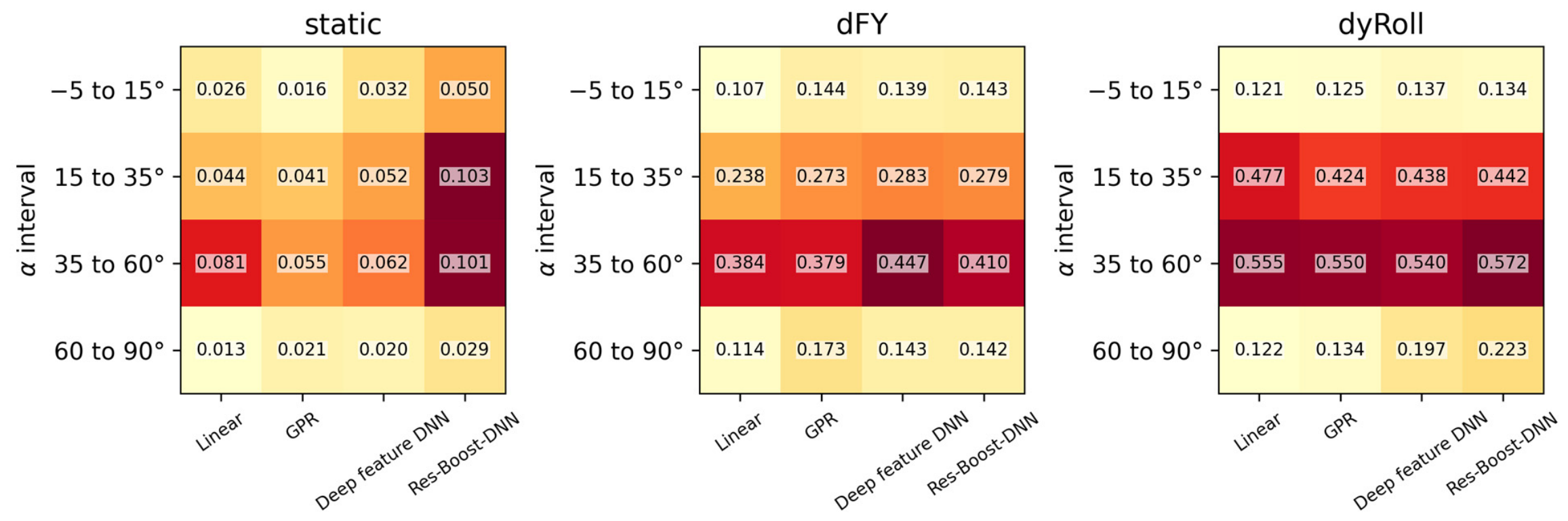
Table A8.
Errors in local slopes with respect to and right-elevator deflection relative to full-table lookup. Results summarize seven conditions at , using a finite-difference step. Errors are expressed in .
Table A9.
Maximum absolute normalized component errors across test nodes and five partitions at the largest training budgets. Coordinates are , and, for dFY, , expressed in degrees. Normalization uses the corresponding component’s training-set standard deviation within each partition.
Figure A5.
Constructive zero-consistency designs separate full-domain accuracy from zero-plane error. Shared neural variants use identical four-candidate validation searches; the zero-plane interpolant adds analytically known zero constraints rather than new measured labels.
References
- Liao, Y.; Cheng, K.; Sun, W.; Zhao, Y.; Jia, X.; Qi, W. Computational fluid dynamics analysis of aerodynamic characteristics in long-endurance unmanned aerial vehicles. Heliyon 2024, 10, e38804. [Google Scholar] [CrossRef] [Scilit] [PubMed]
- Orozco, C.; Vásquez, S.; Caratt, J.; De Armas, N.; Guarín, A. CFD-Based Study of Aerodynamic Performance in UAVs under Adverse Pressure Gradient Conditions. Procedia Comput. Sci. 2025, 257, 1213–1220. [Google Scholar] [CrossRef] [Scilit]
- Utomo, M.S.K.T.S.; Yohana, E.; Mahendra, C.; Utama, I.Y. Analysis of blended winglet parameters on the aerodynamic characteristics of NXXX aircraft using Computational Fluid Dynamics (CFD). Results Eng. 2024, 24, 102901. [Google Scholar] [CrossRef] [Scilit]
- Ejeh, C.J.; Akhabue, G.P.; Boah, E.A.; Tandoh, K.K. Evaluating the influence of unsteady air density to the aerodynamic performance of a fixed wing aircraft at different angle of attack using computational fluid dynamics. Results Eng. 2019, 4, 100037. [Google Scholar] [CrossRef] [Scilit]
- Di, Y.J.; Chen, Z.L.; Su, L.J. Aerodynamic Characteristics of Tail-sitter VTOL UAVs Based on CFD Method. Command Control Simul. 2021, 43, 107–114. [Google Scholar] [CrossRef]
- Nicolosi, F.; Della Vecchia, P.; Ciliberti, D.; Cusati, V. Fuselage aerodynamic prediction methods. Aerosp. Sci. Technol. 2016, 55, 332–343. [Google Scholar] [CrossRef] [Scilit]
- Ishak, H.; Nuhash, A.A.; Jubaer, M.A.G.; Bakaul, S.R. Aerodynamic and Performance Analysis of a Supersonic Next-Generation UCAV Using Hybrid Methodology. In Proceedings of the AIAA 2025 Region VII Conference, Sydney, Australia, 1–2 December 2025; p. 106593. [Google Scholar] [CrossRef] [Scilit]
- Liu, D.; Jin, Z.; Peng, X.; Liu, G.; Zhang, Y. Refined Aerodynamic Test of Wide-Bodied Aircraft and Its Application. Comput. Model. Eng. Sci. 2023, 136, 2691–2713. [Google Scholar] [CrossRef] [Scilit]
- Tang, W.; Huang, Y.; Fu, H. Effect of thrust vector on dynamic aerodynamic characteristics of aircraft at high angle of attack. Acta Aeronaut. Astronaut. Sin. 2018, 39, 121648. [Google Scholar] [CrossRef]
- Wu, J.; Wei, Z.; Liu, Y.; Zhong, M.; Yang, F.; Yu, Y. Civil aircraft standard model system and construction of aerodynamic subject database. Acta Aeronaut. Astronaut. Sin. 2025, 46, 132030. [Google Scholar] [CrossRef]
- Liu, L.; Xiang, X.; Zhang, Y.; Chen, H.; Wei, C.; Zhu, J.; Yang, P. A high lift-to-drag ratio unconventional blended-wing-body aerodynamic configuration with swallow tail. Acta Aeronaut. Astronaut. Sin. 2024, 45, 629630. [Google Scholar] [CrossRef]
- Wu, J.; Qin, Y.; Huang, Z.; Wei, Z.; Jia, Y. Low speed experiment on longitudinal and lateral aerodynamic characteristics of the low aspect ratio flying wing calibration model. Acta Aerodyn. Sin. 2016, 34, 125–130. [Google Scholar] [CrossRef]
- Wang, Y.; Shen, Y.; Bu, C.; Feng, S.; Chen, H.; Tang, W. Research on High Angle of Attack Aerodynamic Characteristics of Low Aspect Ratio Flying Wing. Aerodyn. Res. Exp. 2023, 1, 64–69. Available online: https://pubs.cstam.org.cn/article/id/7854093a-9fd3-4077-9ca3-d6132e7d230a (accessed on 15 November 2026).
- Li, T.; Si, H.; Qiu, J.; Li, J.; Gong, Y. A hybrid algorithm of TCN-iTransformer for aircraft aerodynamic parameter estimation based on dual attention mechanism. Aerosp. Sci. Technol. 2025, 164, 110350. [Google Scholar] [CrossRef] [Scilit]
- Dong, W.; Wang, X.; Han, D.; Lin, Q. Unsteady aerodynamic modeling and analysis of aircraft model in multi-DOF coupling maneuvers at high angles of attack with attention mechanism. Chin. J. Aeronaut. 2025, 38, 103444. [Google Scholar] [CrossRef] [Scilit]
- Lin, H.; Wang, X.; Zhang, W. Transferable scaling function learning method for knowledge embedded aerodynamic database construction. Aerosp. Sci. Technol. 2026, 176, 112097. [Google Scholar] [CrossRef] [Scilit]
- Yan, M.; Liu, K.; An, S.; Wang, G.; Jin, Z.; Zang, J. Transfer learning-driven adaptive physics-informed neural networks acceleration method for aerodynamic identification. Eng. Appl. Artif. Intell. 2026, 166, 113589. [Google Scholar] [CrossRef] [Scilit]
- Lin, H.; Wang, X.; Zhang, W. Scaling function learning: A sparse aerodynamic data reconstruction method for various aircraft shapes. Chin. J. Aeronaut. 2026, 39, 103797. [Google Scholar] [CrossRef] [Scilit]
- Qian, W.; Zhao, T.; Huang, Y.; He, L.; Duan, G.; Qin, C. Modeling and data mining of engineering airfoil aerodynamic characteristics. Acta Aerodyn. Sin. 2021, 39, 175–183. [Google Scholar] [CrossRef]
- He, L.; Qian, W.; Wang, Q.; Chen, H.; Yang, J. Applications of machine learning for aerodynamic characteristics modeling. Acta Aerodyn. Sin. 2019, 37, 470–479. [Google Scholar] [CrossRef]
- Rasmussen, C.E.; Williams, C.K.I. Gaussian Processes for Machine Learning; MIT Press: Cambridge, MA, USA, 2006. [Google Scholar] [CrossRef] [Scilit]
- Friedman, J.H. Greedy function approximation: A gradient boosting machine. Ann. Stat. 2001, 29, 1189–1232. [Google Scholar] [CrossRef] [Scilit]
- Forrester, A.I.J.; Sóbester, A.; Keane, A.J. Multi-fidelity optimization via surrogate modelling. Proc. R. Soc. A Math. Phys. Eng. Sci. 2007, 463, 3251–3269. [Google Scholar] [CrossRef] [Scilit]
- Jones, D.R.; Schonlau, M.; Welch, W.J. Efficient Global Optimization of Expensive Black-Box Functions. J. Glob. Optim. 1998, 13, 455–492. [Google Scholar] [CrossRef] [Scilit]
- Raissi, M.; Perdikaris, P.; Karniadakis, G.E. Physics-informed neural networks: A deep learning framework for solving forward and inverse problems involving nonlinear partial differential equations. J. Comput. Phys. 2019, 378, 686–707. [Google Scholar] [CrossRef] [Scilit]
- McKay, M.D.; Beckman, R.J.; Conover, W.J. Comparison of Three Methods for Selecting Values of Input Variables in the Analysis of Output from a Computer Code. Technometrics 1979, 21, 239–245. [Google Scholar] [CrossRef] [Scilit]

Disclaimer/Publisher’s Note: The statements, opinions and data contained in all publications are solely those of the individual author(s) and contributor(s) and not of MDPI and/or the editor(s). MDPI and/or the editor(s) disclaim responsibility for any injury to people or property resulting from any ideas, methods, instructions or products referred to in the content. |
© 2026 by the authors. Licensee MDPI, Basel, Switzerland. This article is an open access article distributed under the terms and conditions of the Creative Commons Attribution (CC BY) license.