


Abstract
With the introduction of supercooled large droplet (SLD) conditions into international airworthiness standards, numerical prediction and experimental validation of SLD icing have become major challenges in aircraft icing certification. The Lagrangian approach explicitly tracks individual droplet trajectories, allowing size-dependent corrections to aerodynamic drag and droplet–surface interactions to be incorporated directly. However, three-dimensional Lagrangian simulations require tracking large numbers of particles and are difficult to parallelize efficiently, resulting in high computational costs that limit their engineering applications. This study proposes a Particle-Decomposition Parallel Lagrangian (PDPL) framework. Droplet drag is evaluated using the Clift model, while splashing mass loss at the primary impact is accounted for using a LEWICE-style correction. Instead of retaining the mesh partitioning used for airflow computations, the proposed framework employs MPI-3 shared-memory windows to provide all MPI processes within the same compute node with read-only access to the complete mesh and background-flow data, avoiding the substantial increase in memory consumption caused by data replication. Each process independently computes its assigned droplet trajectories without interprocess particle migration, avoiding the communication overhead associated with frequent particle transfers. Surface water-collection efficiency is calculated using a statistical Monte Carlo method from wall-impact contributions accumulated locally and aggregated through MPI. Comparisons with experimental measurements and numerical reference solutions show that the method reproduces the principal collection-efficiency profiles and impingement limits across the configurations considered, with local discrepancies remaining in some cases. Strong-scaling tests demonstrate that the PDPL framework reduces droplet-tracking time as the number of compute nodes increases and supports efficient parallel computation on distributed-memory systems.
1. Introduction
When an aircraft flies through clouds with supercooled water droplets, ice may form on all windward surfaces. This can directly threaten flight safety. Therefore, aircraft icing has long been a key research topic in the aviation field. In particular, in 2015, the Federal Aviation Administration (FAA) introduced Amendment 25–140 for aircraft and Amendment 33–34 for engines. Amendment 25–140 added Appendix O to 14 CFR Part 25, defining supercooled large droplet (SLD) icing conditions and establishing corresponding certification requirements for certain transport-category airplanes. The European Union Aviation Safety Agency (EASA) has also adopted similar requirements [1]. These changes bring new challenges to current numerical icing simulations and wind-tunnel tests.
With the development of mathematical and physical methods and the improvement of computer performance, numerical simulations have been playing an increasingly important role in aircraft icing research. After many years of development, a multistep quasi-steady icing simulation framework has been developed. This framework includes grid generation, flow-field calculation, droplet-field calculation, ice accretion, and grid reconstruction, and has become a common approach in the aviation-safety field. Among these steps, droplet-field calculation is a key part. The accuracy of droplet motion in the flow field and droplet impingement on solid surfaces directly determines the mass flux of freezable water in the later ice-accretion process. At present, the main methods for droplet-field calculation are the Eulerian and Lagrangian methods. In the Eulerian method, the droplet phase is treated as a continuous medium and solved based on control volumes. As the numerical framework of the Eulerian method is similar to that of CFD solvers and is easier to parallelize, it has been widely used in large-scale three-dimensional (3D) icing simulations, such as FENSAP-ICE [2]. The Eulerian method is commonly used to predict droplet impingement characteristics under conventional icing conditions. However, supercooled large droplet (SLD) icing involves freezing drizzle with droplet diameters of 100–500 μm and freezing rain with droplet diameters of 500–2000 μm [1], while mixed-phase icing may also involve the melting and refreezing of ice crystals [3]. Owing to their larger size and greater inertia, SLDs may undergo deformation and breakup during transport, as well as splashing, rebound, and secondary-droplet generation upon impact. Such particle-scale processes are difficult to fully represent using conventional Eulerian methods, potentially limiting the accurate prediction of droplet impingement and secondary impingement. In contrast, the Lagrangian method tracks individual particles, providing a more direct framework for describing droplet motion and interactions with surfaces. When coupled with appropriate physical models, it can account for these complex processes, as well as the melting and refreezing of ice crystals. Therefore, the Lagrangian method has become increasingly important in SLD icing research.
The current research on the Lagrangian method mainly focuses on the following three aspects. The first aspect is the improvement of prediction accuracy. Wang et al. [4] proposed a semi-empirical splashing and reimpingement model for Lagrangian trajectory tracking. They also verified its ability to predict water collection efficiency under typical icing conditions. Ren et al. [5] used adaptive refinement based on Cartesian grids to improve the identification of 3D droplet impingement limits. They also used radial basis function (RBF) interpolation to improve the representation of water collection efficiency on 3D surfaces. Later, to reduce interpolation-induced errors in the collection-efficiency calculation, they further proposed a gradient-descent-based method [6]. Han et al. [7] developed a particle-statistics-based method for water-collection efficiency within the Lagrangian framework. This method avoids the limitations of the traditional stream-tube method in 3D calculations. It also extends the Lagrangian method to complex geometries and unsteady simulations.
The second aspect is the improvement of computational efficiency. Rendall and Allen [8] proposed a finite-volume-based droplet-trajectory method. They extended the streamline representation to droplet-governing equations. They also used grid connectivity to advance droplet trajectories efficiently between mesh cells. In this method, the original connectivity of the CFD grid was used to track a particle from one cell to its neighboring cell. Thus, a droplet could be advanced within each mesh cell using only one integration step. This avoided the frequent global particle location and containment checks in the traditional Lagrangian method. This technique greatly reduced the computing time for a single droplet trajectory. Xie et al. [9] proposed an improved framework based on a new delta form, adaptive mesh refinement (AMR) for the release grid, and constrained RBF interpolation. This framework could achieve accuracy similar to that of a large-particle simulation by tracking only a small number of particles. It was implemented in a serial manner. By reducing the dependence on high-density particle sampling in complex 3D cases, this framework greatly reduced the computing time for water-collection-efficiency prediction. Liu et al. [10] combined a Monte Carlo Lagrangian droplet solver with a backpropagation (BP) neural network. They also used an OpenMP parallel strategy to improve the efficiency of water-collection-efficiency calculation in 3D aircraft icing simulations through asynchronous parallel computing. With 16 threads, they computed the droplet-impingement characteristics of the GLC-305 swept wing and an engine nacelle. The two cases tracked 1M and 4M particles and required over 2546 and 3896 s, respectively. Compared with the algorithm without the BP neural network, the computing time was reduced by 26.8% and 24.5%, respectively.
The third aspect is the development of parallel methods to improve the scalability of Lagrangian particle tracking. Baldan et al. [11,12] introduced particle-informed mesh repartitioning, using representative trajectories to weight the mesh according to particle-crossing frequency. This strategy directs more computational resources to regions with substantial tracking work and improves performance within a spatially decomposed framework. It also illustrates the importance of balancing particle workload, which need not follow the distribution of mesh cells [11,12].
More recently, Zayni et al. [13] developed a ray-tracing-enhanced Lagrangian framework in CHAMPS. Their method combines face-to-face tracking with bilinear-patch intersections for quadrilateral faces, adaptive seeding, and neighboring-face interpolation of collection efficiency. Local streamtubes are reconstructed using a primary trajectory and two auxiliary trajectories. The implementation couples spatial domain decomposition with node-local mesh sharing and demonstrates effective scaling across compute nodes. These developments improve geometric traversal and deposition estimation while emphasizing the roles of both local tracking algorithms and parallel organization. However, node-local mesh sharing alone does not eliminate the communication required for droplet tracking across spatial partitions on different compute nodes.
The present work focuses on the storage and execution of large particle populations. Instead of assigning tracking work according to spatial mesh partitions, a complete trajectory is treated as an independent task. Each compute node stores a shared, complete set of read-only mesh and background-flow data, allowing its processes to follow particles throughout the domain. Consequently, particle ownership remains unchanged during cell traversal, eliminating interprocess particle migration and its associated communication overhead. Wall-impact contributions are aggregated across nodes at sampling synchronization points; MPI collectives are also used for particle initialization, control, and numerical checks. Sharing these data arrays within each node reduces data replication among its processes, while distributing particle tasks across nodes enables efficient parallel tracking of large particle populations.
On this basis, a Particle-Decomposition Parallel Lagrangian (PDPL) framework is developed in the LASA-List BX icing-simulation platform. Surface water-collection efficiency is calculated using a Monte Carlo method based on weighted particle-impact statistics. MPI communication combines wall contributions across nodes, preserving a common statistical estimate as the process count changes. The framework is assessed through comparisons with experimental and numerical reference data and fixed-workload strong-scaling tests.
2. Numerical Methodology
2.1. Background Flow Field and Lagrangian Method
In this work, three-dimensional droplet transport and impingement are predicted within a Eulerian–Lagrangian framework. The background airflow is computed using the finite-volume solver implemented in the LASA-List BX platform, which solves the compressible Reynolds-averaged Navier–Stokes equations with the SST k–ω turbulence model. Convective fluxes are evaluated using the HLLC scheme with second-order spatial reconstruction, and the steady-flow calculation employs implicit backward-Euler pseudo-time marching. A uniform freestream is prescribed at the inlet, a static-pressure boundary condition is imposed at the outlet, and no-slip conditions are applied at solid surfaces. The resulting nodal flow data, together with the mesh geometry and connectivity, are supplied to the Lagrangian solver. Droplet trajectories are then integrated in the prescribed airflow, and the surface collection-efficiency distribution is determined from the droplet-impingement statistics.
The governing equation for droplet motion in the Lagrangian method is given as follows:
where ρa and ρd denote the air and droplet densities, respectively, Vd is the droplet volume, Ap is the projected frontal area, ua is the local gas velocity at the droplet position, and ud is the droplet velocity, and g is the gravitational acceleration vector. The droplet velocity is calculated using the classic fourth-order Runge–Kutta method, while the droplet position is updated using the trapezoidal rule:
where and represent the position and velocity of the droplet at step n, respectively, and Δtn is the corresponding physical time interval for that step.
The integration of water droplet trajectories employs a local variable time step to adapt the temporal resolution to the current grid scale and the water droplet’s motion state. Based on the characteristic length of the host cell and the local reference velocity, the characteristic time required to traverse the current cell is estimated as follows:
where is the characteristic length of the current element, and Uε is a small positive number chosen to avoid division by zero. Additionally, to prevent crossing a cell in a single step, the time step is limited to:
At the same time, the effective relaxation time is used to characterize how quickly the droplet velocity responds to the local airflow:
In this equation, d is the droplet diameter, μa is the aerodynamic viscosity, and CD is the drag coefficient. One-fourth of the effective relaxation time is taken as the relaxation time step limit, which, together with the grid time step limit and the global maximum step size, determines the local upper limit:
Therefore, smaller cell sizes or higher local velocities impose stricter constraints on the time step size, while shorter relaxation times impose stricter temporal constraints on the droplet velocity response process. The actual time step size used in the current step is obtained by clipping the candidate value within local upper and lower bounds:
where Δtn,candidate represents the suggested time step for this step; for the first step, it is provided by the initialization, while for subsequent steps, it is adjusted based on the displacement feedback from the previous step. is the lower bound for the current time step, which prevents the time step from becoming too small. In this study, it is set to 5 × 10⁻⁶ s.
After predicting the position of the water droplet at time step n + 1, calculate the relative displacement ratio:
A target displacement ratio of 0.12 is used to adjust the time step size, balancing local trajectory resolution with computational cost:
where ε = 10−8, to ensure a smooth variation in the candidate step size, the adjustment factor derived from the displacement feedback is restricted to the range of 0.5–1.6. This setting allows for a relatively rapid reduction in the step size when the predicted displacement is too large, while imposing a conservative limit on step size increases to mitigate abrupt changes during adaptive adjustment. The factor limitation is applied only to the generation of the next candidate value:
To improve the prediction of SLD trajectories, deformation effects on the drag coefficient are considered through the Clift model [14]. In this model, a deformed droplet is assumed to exhibit an aerodynamic response intermediate between that of a sphere and disk, and the corresponding weighting is determined by the Weber number. The corrected drag coefficient is expressed as
where Cd,sphere and Cd,disk are defined as
and the interpolation coefficient fm is given by
2.2. MPI-3 Shared-Memory Parallel Strategy
Particle decomposition assigns complete droplet trajectories to MPI processes independently of the mesh partition. Each process therefore requires access to the full mesh and background flow, even though it advances only a subset of the particles. Storing these data separately on every process can make memory demand grow with the process count. The PDPL framework addresses this cost by sharing the read-only data among processes on the same compute node.
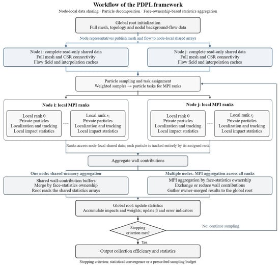
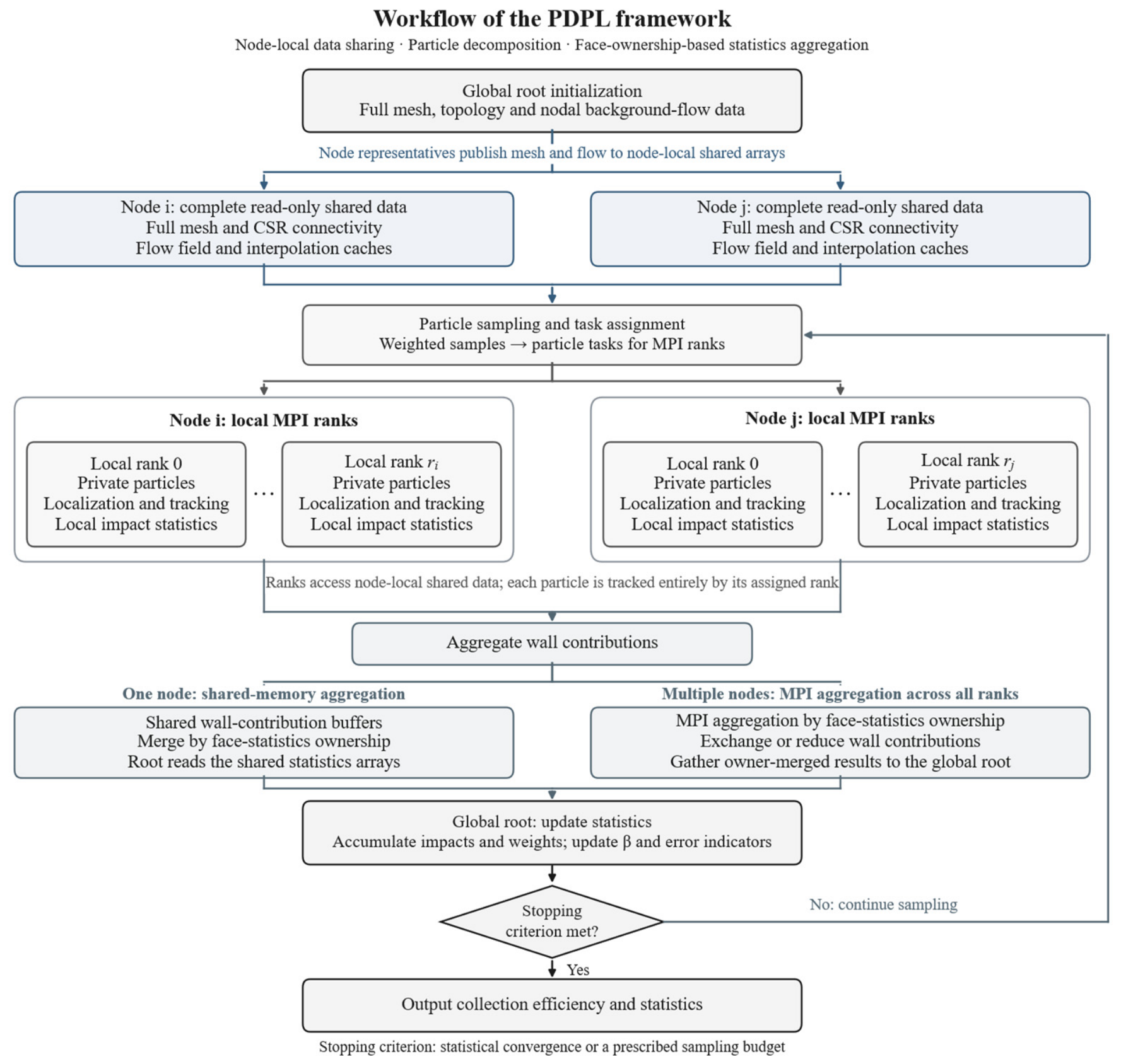
Figure 1 outlines the PDPL framework workflow. The global root process prepares the mesh topology and nodal background-flow data. Mesh coordinates, cell and face connectivity, and flow data are organized into read-only arrays, with connectivity stored in compressed sparse row (CSR) form. The arrays are distributed among node representatives, which publish one copy in an MPI-3 shared-memory window on each node. All processes on a node can then access the same complete data set. Each compute node holds its own shared copy.
Figure 1.
Overall workflow of the Particle-Decomposition Parallel Lagrangian (PDPL) framework. Wall statistics are updated at sampling synchronization points; the loop ends when the convergence criterion or prescribed particle budget is reached.
The PDPL framework utilizes MPI-3 shared memory to enable processes within the same compute node to jointly access a complete set of grid and background flow field data. The shared data is initialized prior to tracking, synchronized within the node, and made available to all processes for read-only access; it is reused across different sampling batches. Each process independently maintains particle states and local wall statistics, thereby reducing redundant storage while preserving the independence of trajectory calculations. Inter-process particle tasks are distributed via MPI, while local trajectory calculations, cache construction, and wall field post-processing support OpenMP parallelization.
Particle samples are distributed among the MPI processes, and each process advances its assigned trajectories using the node-local shared data. A particle remains with the same process as it crosses mesh cells, so trajectory advancement requires no transfer of particle states between processes. Wall-impact contributions are aggregated at sampling synchronization points to update the collection-efficiency distribution and assess convergence. Single-node calculations combine these contributions through shared memory, while multi-node calculations use MPI communication.
Let Ms denote the memory required by one complete set of read-only mesh and flow arrays, and let mr denote the private particle and local-statistics storage of process r. For n compute nodes with q MPI processes per node, the total process count is P = nq. The leading storage requirements of per-process replication and node-local sharing can then be expressed as
and
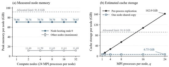
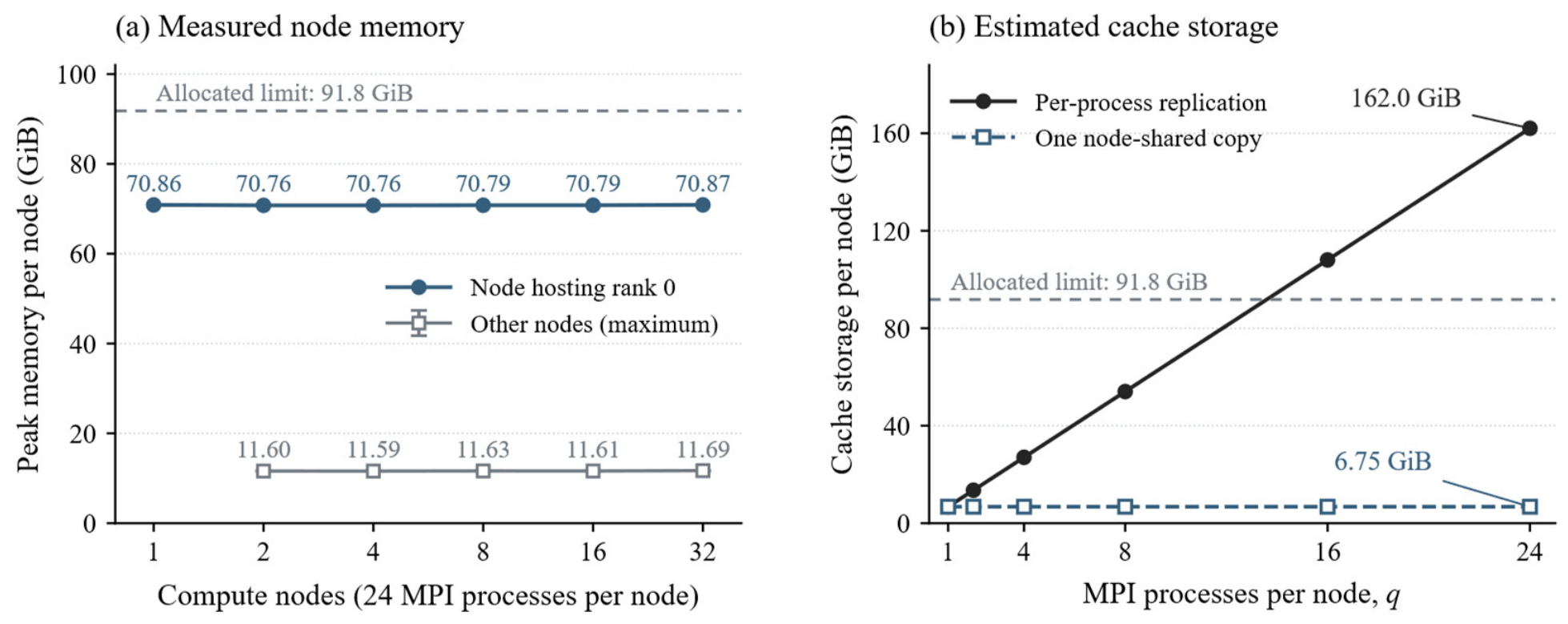
The auxiliary terms include aggregation workspaces, MPI storage, and additional root-owned mesh and result data. Their sizes depend on the implementation and workload, as does the private storage of each process. The reduction in replication is isolated in Figure 2.
Figure 2.
Memory consumption for the 16.75-million-cell horizontal-tail mesh: (a) measured node-level peak memory with 24 MPI processes per node; (b) estimated cache storage under node-local sharing and per-process replication. Gray dashed lines indicate the allocated memory limit per node.
Figure 2a presents the measured memory consumption for the 16.75-million-cell horizontal-tail mesh used in the scalability study. With 24 MPI processes per node, the recorded peak memory ranges from 70.76 to 70.87 GiB on the node-hosting rank 0 and from 11.59 to 11.69 GiB on the other nodes. These values represent the cgroup memory high-water marks for node jobs during the initialization and first particle-tracking phases under different parallel configurations. Since the root process retains additional initialization data, the memory requirements for the node hosting that process are higher.
Figure 2b illustrates the storage requirement associated with per-process replication using the reported cache arrays. Under per-process replication, each MPI process independently stores a cache copy of approximately 6.75 GiB. Consequently, 24 processes on a single node would require approximately 162.0 GiB for these caches alone, exceeding the per-node memory allocation of 91.8 GiB used in this study. This storage requirement increases linearly with the number of processes on a node, limiting both the process count and the mesh size that can be accommodated. The PDPL framework avoids this duplication by allowing processes within each node to access a single shared cache copy.
2.3. Particle-Decomposition-Based Independent Tracking
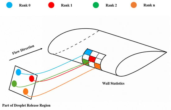
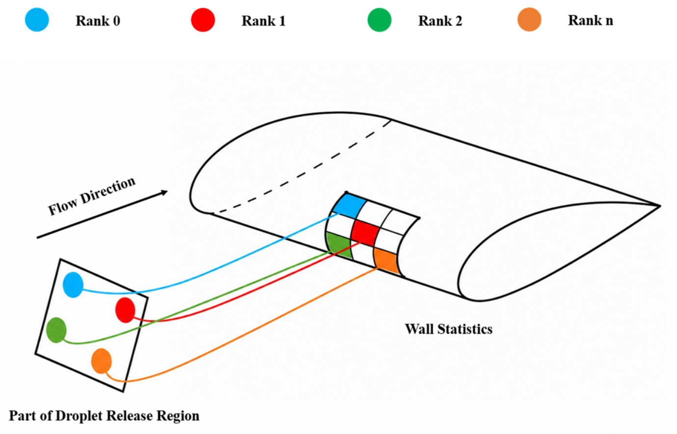
After memory-management improvement, the core focus of the task-parallel Lagrangian method becomes particle distribution and independent droplet-trajectory calculation. The release setup used in the present solver is presented schematically in Figure 3.
Figure 3.
Particle release and independent trajectory tracking in the PDPL framework. Colors identify particles assigned to different MPI ranks.
A relatively broad release region is initially specified to cover potential impinging trajectories. In the adaptive release-region procedure, the initial positions of droplets that impinge on the surface are used to identify an effective upstream release envelope. The release boundaries are gradually adjusted towards this envelope, retaining an empirical margin equal to 10% of its span on each side in the corresponding direction. This margin reduces the risk of excluding marginal impinging trajectories, while adjustment of the release region reduces the computational cost associated with non-impinging particles. The procedure is repeated as further impingement information becomes available, balancing trajectory coverage and computational efficiency. The agreement with reference impingement limits in Section 3.2, including the two SLD conditions for the NACA23012 airfoil and the comparisons across different geometries, supports adequate release-region coverage over the conditions investigated.
Each droplet parcel contains its initial position, initial velocity, droplet size, and weight. These droplet parcels are then assigned to different MPI ranks according to the parallel task division. In Figure 3, circles of different colors represent droplet parcels assigned to different ranks. Each rank advances its own droplets alone. During trajectory tracking, the state of each droplet does not need to be exchanged with other ranks. When a droplet moves in the air-flow field, it obtains the local gas phase velocity near its current position from the shared mesh and shared flow-field data. Then, its trajectory is integrated step-by-step. After a droplet hits the wall surface, the corresponding rank records the impacted face ID, its contribution to the water-collection efficiency, the sample weight, and deposition contribution after splash correction in its local statistics. If a droplet does not hit the wall, and leaves the computational domain, its trajectory calculation is terminated.
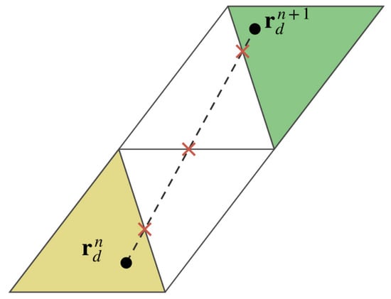
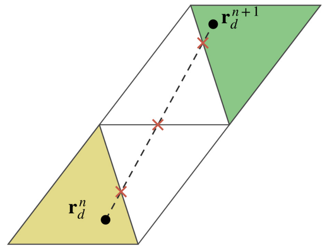
During droplet-trajectory integration, a droplet trajectory segment may cross one or more cell boundaries within a single integration step. In the present implementation, once a droplet leaves its current host cell, the remaining part of the trajectory segment is traced continuously through neighboring cells, following the geometric traversal procedure described by Bellosta et al. [12]. This process continues until the droplet exits the computational domain or impacts a solid wall. Through this cell-by-cell tracking approach, the algorithm can identify the next mesh cell entered by the droplet while simultaneously detecting whether the droplet impacts a solid wall. As shown in Figure 4, after the droplet position at time step n + 1 is predicted, the trajectory segment from rdn to rdn+1 is traced cell-by-cell, starting from the current host cell. Each time the segment crosses an internal face, the algorithm switches to the neighboring cell using the mesh connectivity and continues tracing the remaining segment. Once the predicted position is reached, the next integration step is performed. This treatment improves the robustness of trajectory calculation in complex meshes and reduces the possibility of missing impact events during repeated cell crossings.
Figure 4.
Schematic illustration of a particle moving across neighboring cells from its position at time step n (rdn) to its position at time step n + 1 (rdn+1) within one integration step. Black dots indicate the particle positions at time steps n and n + 1, respectively; the dashed line represents the particle trajectory; red crosses mark the intersections of the trajectory with cell faces; and the yellow and green regions denote the cells containing the particle at time steps n and n + 1, respectively.
2.4. Statistics-Based Monte Carlo Method for Water Collection Efficiency
After trajectory advancement and wall-impact detection, each MPI process accumulates local face-based impingement contributions. These contributions are aggregated by wall-face ownership through shared memory or MPI to construct the collection-efficiency field. To improve the generality of the numerical framework and extend its applicability to water-collection prediction on complex 3D geometries, the conventional streamtube formulation is replaced by a particle-based Monte-Carlo statistical approach [10]. In this approach, droplet release positions are sampled from a prescribed far-upstream plane, whose extent is adaptively adjusted according to the limiting impingement range inferred from the current wall-impact statistics.
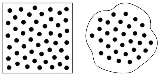
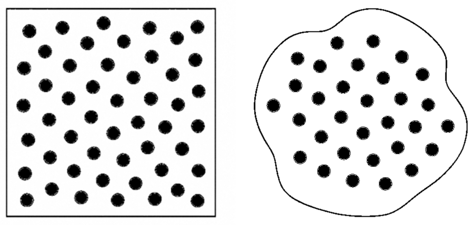
As illustrated schematically in Figure 5, the square region represents the upstream release plane, whereas the enclosed irregular region represents the subset of release locations whose trajectories eventually contribute to a given wall face or wall patch. From this viewpoint, the wall-collection efficiency is evaluated statistically from the distribution of particle impacts induced by the release-plane sampling, rather than from a conventional streamtube argument.
Figure 5.
Monte Carlo interpretation of face-based collection efficiency. The square represents the upstream droplet release plane, with black circles indicating the droplet release locations. The enclosed region represents the droplet impingement area on the wall, and the black circles within it indicate the final impingement locations of the droplets.
Accordingly, the wall-collection efficiency can be interpreted as the expectation of the wall-impact contribution induced by a random initial droplet position on the upstream release plane. Let denote the release plane with area AR, and let f be a wall face with area Af. For a release position , the droplet released from y is advanced along its Lagrangian trajectory, and may either impinge on face f or miss it. If the droplet eventually impinges on face f, its local contribution is defined as
where is the representative mass flux of the released sample, LWC is the liquid water content, and U∞ is the freestream velocity. If no impact occurs on face f, the contribution is taken as zero. The collection efficiency on face f is therefore given by the expectation of this local contribution under the target release distribution on .
For a uniform target distribution on the release plane
The Monte Carlo estimator of the face-based collection efficiency is
To improve statistical efficiency, non-uniform sampling may also be employed. Let the actual sampling distribution be q(y). An unbiased correction is then introduced through the sample weight
The representative mass flux associated with sample p can be expressed as
If sample p eventually impinges on wall face f, its local contribution becomes
Further introducing the impact indicator function
the weighted Monte Carlo estimator of the collection efficiency on face f can be written as
Therefore, the computation of water-collection efficiency in the present solver can be interpreted as a statistical procedure in which the initial droplet positions on the release plane are sampled randomly or quasi-randomly, the wall-impact contributions of each sample are treated as random variables, and the expected wall-collection efficiency is approximated by the sample average. When Sobol low-discrepancy points are used, the method can be more precisely interpreted as a weighted quasi-Monte-Carlo approach; when uniform random sampling is adopted, it corresponds to the classical Monte-Carlo method.
2.5. Splash Correction for SLD Impact
When SLDs impinge on a solid surface, splashing may occur, leading to partial mass loss and a corresponding reduction in the local water collection. To account for this effect, a LEWICE-style splash correction is introduced. The model follows the framework developed by Wright et al. [15], in which splashing behavior is correlated with the local impact conditions and impact angle.
The critical threshold for droplet splashing upon impact is given by
where K is the critical splashing threshold proposed by Mundo et al. [16]
and f* is the impact frequency, defined as
Here, Oh the Ohnesorge number, Wen is the normal Weber number, and LWC is the liquid water content.
Based on these quantities, the splash factor S is evaluated as
where Kcrit is given by
and θ0 is the impact angle between the incoming droplet velocity and the wall tangent.
sinθ0 is defined as
Accordingly, the corrected water collection efficiency, , can be expressed as
In the present study, splashing is represented by a local correction to the water mass retained at the initial impact, without explicitly tracking secondary droplets. For isolated configurations, splashed droplets can be convected downstream without reimpinging on the model, as reported by Bellosta et al. [12]. Under such conditions, the principal influence of splashing on water collection can be represented through the initial mass-loss correction. This treatment therefore provides a reasonable engineering approximation for predicting the main collection-efficiency distribution while avoiding the additional cost of tracking secondary particles. The experimental comparisons presented in this study support its use for the configurations and conditions investigated.
3. Results and Discussion
3.1. Benchmark Cases and Computational Setup
To assess the proposed PDPL framework, a series of benchmark cases was considered to evaluate both predictive accuracy and computational efficiency. The benchmark set included canonical and practical configurations commonly used in aircraft icing and droplet-impingement studies, namely, the NACA0012 and NACA23012 airfoils, a circular cylinder, a sphere, the ONERA M6 swept wing, and the NACA64A008 horizontal tail. The numerical simulations presented in this paper were performed at the Hefei Advanced Computing Center using compute nodes equipped with two AMD EPYC 7742 processors, each with 64 physical cores.
The benchmark conditions are summarized in Table 1. Unless otherwise stated, collection-efficiency distributions were obtained by combining the individual size-bin results according to the weights of a discretized Langmuir-D droplet-size distribution. Sampling continued until the relative change in integrated water collection remained below 10−5 for three consecutive updates.
Table 1.
Benchmark cases and simulation conditions.
3.2. Accuracy Assessment
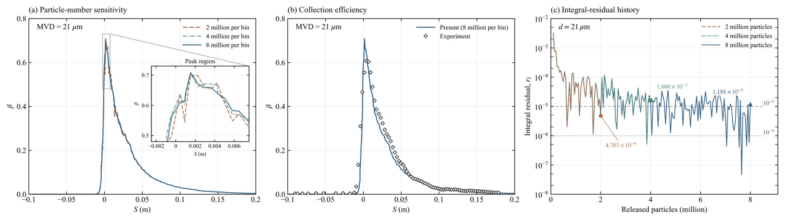
This section presents an assessment of the predictive accuracy of the proposed method, using the benchmark cases listed in Table 1. The numerical results are compared with the available reference solutions and publicly available experimental data from the aircraft icing literature. To investigate the effect of particle number on local peaks and distribution profiles, using the NACA64A008 horizontal tailplane as an example, the mesh, background flow field, release region, and integration parameters were kept constant. A total of 2 million, 4 million, and 8 million particles were released into each size fraction of the Langmuir-D distribution, corresponding to total particle counts of 14 million, 28 million, and 56 million, respectively.
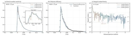
As shown in Figure 6a, the combined collection-efficiency profiles become progressively closer as the particle population increases. The enlarged peak region reveals local fluctuations for 2 million particles per component, whereas the profiles obtained with 4 and 8 million particles nearly coincide over the main impingement region. The relative differences between the latter two calculations are 0.47% for the principal peak and 1.47% for the local peak on the opposite side, indicating that further increases in particle number have a limited effect on the principal sectional features.
Figure 6.
Particle-number sensitivity for the NACA64A008 horizontal tail at MVD = 21 μm. (a) Collection-efficiency profiles for the Langmuir-D distribution with 2, 4, and 8 million particles per size bin. (b) Comparison of the prediction using 8 million particles per size bin with the measurements of Papadakis et al. [17]. (c) Integral-residual histories for monodisperse 21 μm dropletss.
Figure 6b compares the result obtained with 8 million particles per bin with the experimental measurements. The calculation reproduces the main distribution and downstream decay, although the peak is overpredicted and collection efficiency is underpredicted over part of the post-peak region. The small differences between the 4-million- and 8-million-particle profiles indicate that these local discrepancies are relatively insensitive to further increases in particle number.
Figure 6c presents the integral-residual histories for the NACA64A008 horizontal tail at MVD = 21 μm. The residual decreases overall as the particle population increases, with batch-to-batch fluctuations persisting at higher particle counts. The 10−5 criterion is first satisfied for three consecutive sampling updates at approximately 4.85 million particles, whereas the stricter 10−6 criterion is not satisfied for three consecutive updates within 8 million particles. Together with the small changes in the collection-efficiency profiles between 4 and 8 million particles per bin in Figure 6a, these results support the adoption of 10−5 as a practical balance between sampling accuracy and computational efficiency under the conditions examined.
3.2.1. Extruded Wing Sections
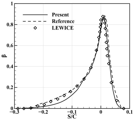
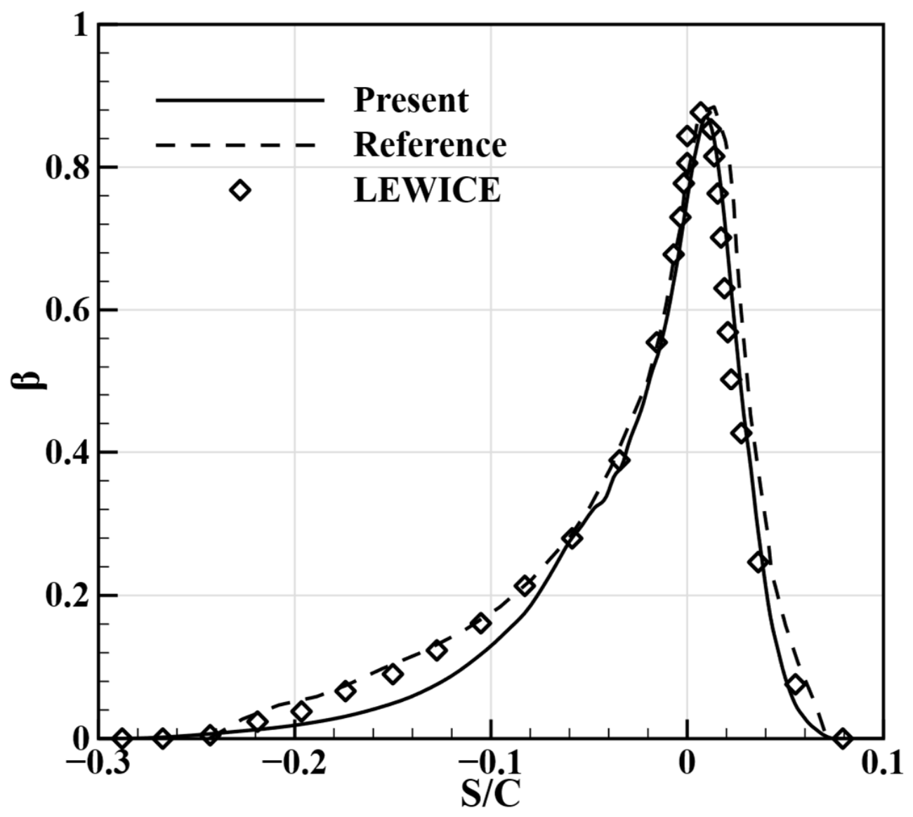
The extruded NACA0012 and NACA23012 sections are considered first to examine droplet impingement under small- and large-droplet conditions, respectively. Figure 7 compares the NACA0012 results with the predictions of Zeng et al. [18] and LEWICE. The present method accurately captures the peak location and impingement limits. The predicted collection-efficiency distribution on the upper surface agrees more closely with the LEWICE results, whereas some discrepancies remain on the lower surface.
Figure 7.
Collection-efficiency distribution on the spanwise-extruded NACA0012 section at U∞ = 102.8 m/s, AOA = 4°, and MVD = 40 μm. The dashed line (Reference) and open diamonds (LEWICE) show the Lagrangian and LEWICE predictions, respectively, reported by Zeng et al. [18]. Here, β denotes the local water collection efficiency (dimensionless). S/C is the sectional coordinate normalized by the airfoil chord C.
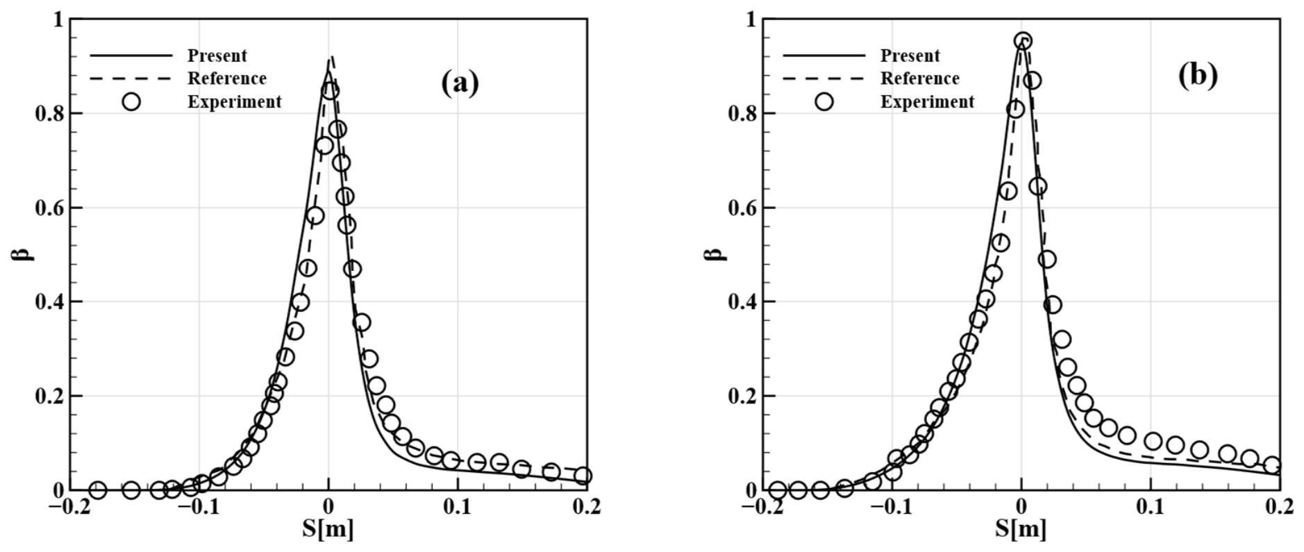
Figure 8 presents the NACA23012 results for MVDs of 111 and 236 μm, together with the experimental measurements and the predictions reported by Bellosta et al. [12]. The asymmetric collection-efficiency distribution and the peak near the stagnation region are captured under both conditions. For an MVD of 111 μm, the present prediction follows the measured peak more closely than the reference calculation, although differences remain on either side. At 236 μm, the peak remains close to the measurements, but collection efficiency is underestimated in the downstream decay region. Overall, for the SLD condition, the present method shows good agreement with the experimental measurements near the peak collection efficiency.
Figure 8.
Collection-efficiency distributions on the spanwise-extruded NACA23012 section at U∞ = 78.232 m/s and AOA = 2.5°. The MVD is 111 μm in (a) and 236 μm in (b). Dashed lines show the predictions of Bellosta et al. [12]. Open circles show the experimental measurements of Papadakis et al., as reported in Figure 8 of the same study [12]. Here, β denotes the local water collection efficiency (dimensionless), and S is the sectional coordinate in meters.
3.2.2. Canonical Bluff Bodies
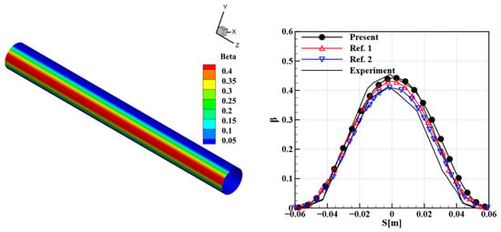
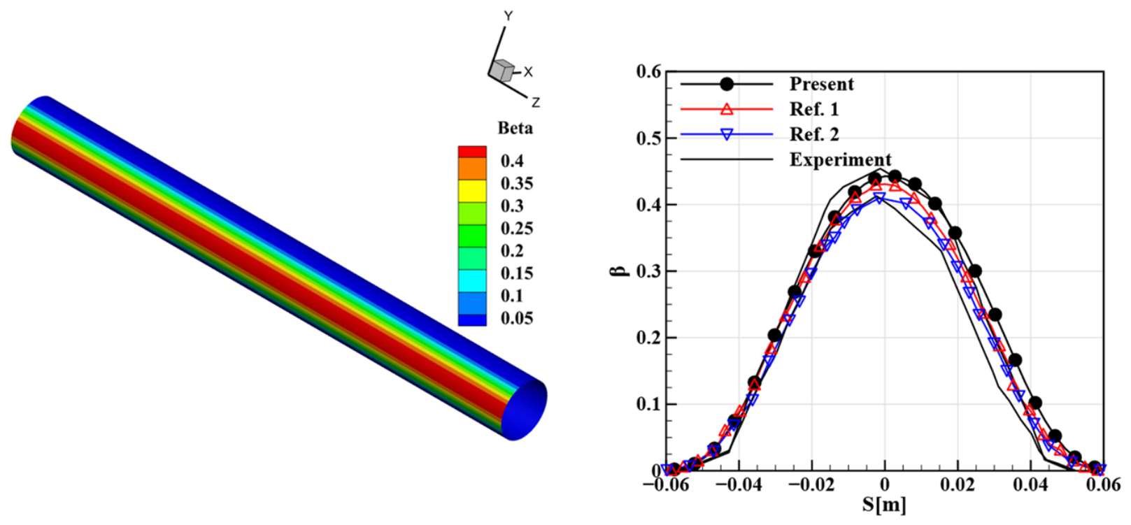
The predictive accuracy of the proposed method is further examined using a circular cylinder and a sphere. Compared with the spanwise-extruded airfoil cases, these two configurations involve more pronounced 3D geometric effects and therefore provide more stringent benchmark cases for validation. For the circular-cylinder case, the computational mesh consists of 477,242 cells. The air density is set to 1.097 kg/m3, and the far-field static pressure is specified as 89,867 Pa. Figure 9 shows the wall collection-efficiency contour together with a comparison between the mid-span sectional distribution and the experimental data.
Figure 9.
Surface collection-efficiency distribution (left) and midspan sectional profile (right) for the circular cylinder at U∞ = 80 m/s and MVD = 16 μm. Ref. 1 (open upward triangles) and Ref. 2 (open downward triangles) denote the predictions of Ren et al. [5] and Xie et al. [9], respectively. The solid black curves without markers show the experimental range reported by Tong and Luke [19]. Here, β denotes the local water collection efficiency (dimensionless), and S is the sectional coordinate in meters.
Figure 9 compares the present prediction with the numerical results of Ren et al. [5] and Xie et al. [9] and the experimental data [19]. The present solution reproduces the main features of the collection-efficiency distribution and accurately captures the impingement limits on both sides. The predicted peak collection efficiency lies close to the upper end of the reported experimental range.
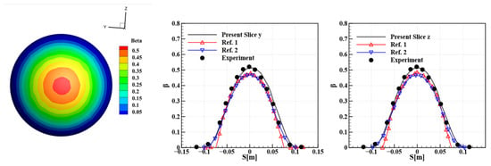
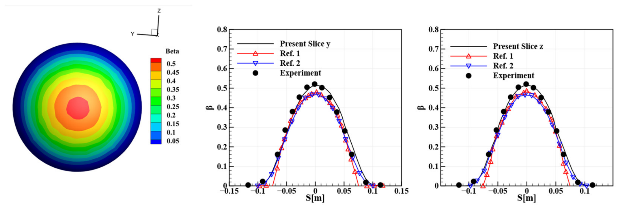
The sphere extends the comparison to a surface with curvature in two directions. Figure 10 shows the surface distribution and profiles along two orthogonal sections, together with the predictions of Ren et al. [5] and Xie et al. [9] and the experimental data reproduced in Ref. [20]. Both sections exhibit similar profiles, with the highest collection efficiency near the stagnation point. The present peak values lie closer to the measurements than the two numerical reference solutions, which underpredict collection in this region. The present profiles also follow the measured decrease away from the peak, with smaller differences remaining toward the impingement limits.
Figure 10.
Surface collection-efficiency distribution and profiles along two orthogonal sections of the sphere at U∞ = 75 m/s and MVD = 18.6 μm. The sections are labeled Slice y and Slice z. Ref. 1 (upward triangles) and Ref. 2 (downward triangles) denote the predictions of Ren et al. [5] and Xie et al. [9], respectively. Filled circles show experimental measurements reproduced by Bidwell and Mohler [20]. Here, β denotes the local water collection efficiency (dimensionless), and S denotes the sectional coordinate in meters.
3.2.3. ONERA M6 Swept Wing and Horizontal Tail
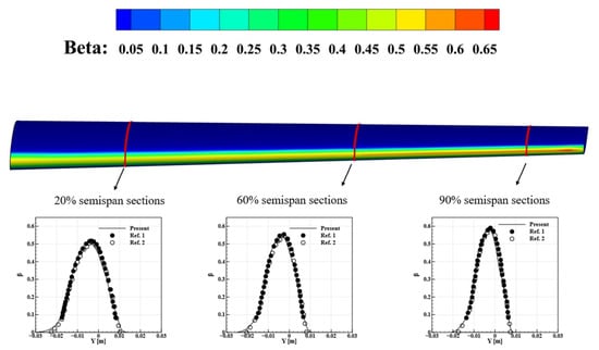
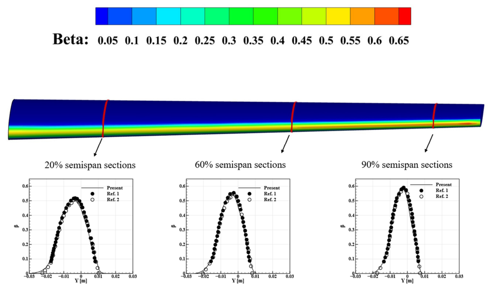
The ONERA M6 swept wing is used to examine spanwise variations in droplet impingement. Figure 11 shows the surface collection-efficiency distribution and profiles at 20%, 60%, and 90% of the semispan. Impingement remains concentrated near the leading edge; toward the outboard sections, the impingement region narrows while the peak collection efficiency increases. The present profiles agree well with the predictions of Sang et al. [21] and Peña et al. [22] at all three stations in peak magnitude, distribution shape, and impingement extent.
Figure 11.
Surface collection-efficiency distribution on the ONERA M6 wing and sectional profiles at 20%, 60%, and 90% of the semispan, at U∞ = 50 m/s, AOA = 6°, and MVD = 20 μm. Ref. 1 (filled circles) denotes the predictions of Sang et al. [21], and Ref. 2 (open circles) denotes those of Peña et al. [22]. Here, β denotes the local water collection efficiency (dimensionless), and Y denotes the sectional coordinate in meters.
Following the ONERA M6 swept-wing case, the proposed method was further assessed on a 3D horizontal-tail configuration, which provides a more practical validation case for aircraft-icing applications. The computational mesh consisted of 2.435 million cells. In this case, the water collection efficiency was evaluated under two droplet conditions with MVDs of 21 μm and 92 μm. The present results were compared with the numerical and experimental data reported in Ref. [12], where the numerical results were given by Bellosta et al. and the experimental measurements were taken from Papadakis [17].
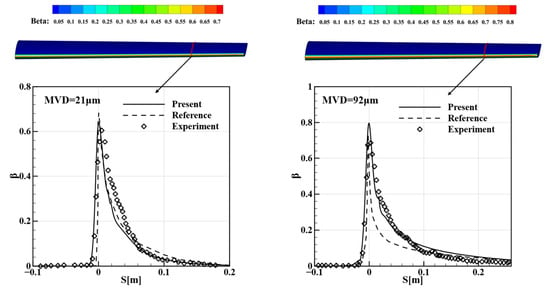
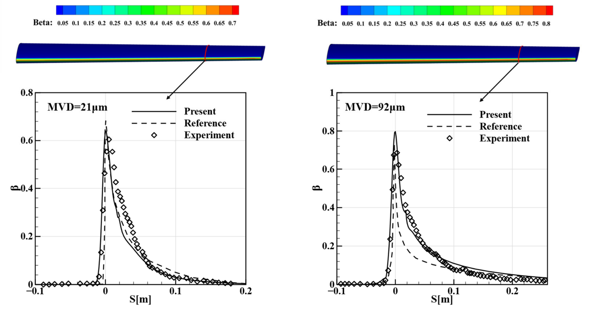
The NACA64A008 horizontal tail provides a further comparison with experimental measurements for MVDs of 21 and 92 μm. Figure 12 presents the profiles at the measurement station located 37 inches above the wind-tunnel floor, together with the predictions of Bellosta et al. [12] and the measurements of Papadakis et al. [17]. The upper-surface impingement limit is reproduced under both conditions. For an MVD of 21 μm, the present peak is closer to the measurements than the reference prediction, and the lower-surface distribution follows the measured decay more closely. At 92 μm, the present prediction continues to follow the measured lower-surface distribution more closely, while the peak collection efficiency is overpredicted, consistent with the trend observed in the reference results of Bellosta et al. [12].
Figure 12.
Surface collection-efficiency distributions and sectional profiles on the NACA64A008 horizontal tail at U∞ = 78.68 m/s and AOA = 6° for MVDs of 21 μm (left) and 92 μm (right). Profiles are taken at the measurement station 37 inches above the wind-tunnel floor. Dashed lines show the reference predictions of Bellosta et al. [12], and open diamonds show the experimental measurements of Papadakis et al. [17]. Here, β denotes the local water collection efficiency (dimensionless), and S denotes the sectional coordinate in meters.
These validation results demonstrate the ability of the proposed task-parallel Lagrangian framework to predict water collection efficiency for a range of three-dimensional configurations, including extruded airfoil sections, curved bluff bodies, swept wings, and horizontal tails. Across the droplet-size conditions considered, the method reproduces the principal features of the collection-efficiency distributions and captures the impingement limits. Although local differences remain, the overall agreement with experimental measurements and numerical reference solutions supports the applicability of the framework to droplet-impingement prediction in aircraft-icing applications.
3.3. Computational Efficiency and Scalability
The parallel scalability of the PDPL framework is evaluated using the NACA64A008 horizontal-tail configuration under the conditions listed in Table 1. The tests employ the official hybrid mesh provided for the First AIAA Ice Prediction Workshop, also adopted by Baldan et al. [11], comprising 16.75 million cells and 3.82 million nodes. A fixed population of one million monodisperse 21 μm droplets is tracked as the number of MPI processes is increased.
The tests are conducted on the previously described high-performance computing cluster at the Hefei Advanced Computing Center. Calculations use one, two, four, eight, 16, and 32 nodes, with 24 MPI processes per node. This choice includes the 24-, 48-, and 96-core allocations reported by Baldan et al. [11] in the comparison. These core counts correspond to one, two, and four nodes in the present tests, which are further extended to 768 processes. Each configuration is repeated three times, and the median computation time is reported. Taking the one-node calculation as the reference, speedup and relative parallel efficiency are defined as and , respectively, where T(n) denotes the median computation time on n nodes.
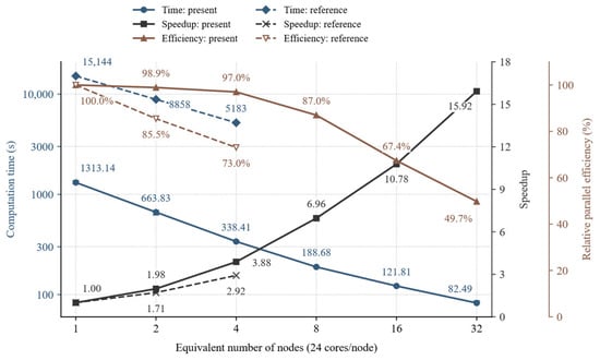
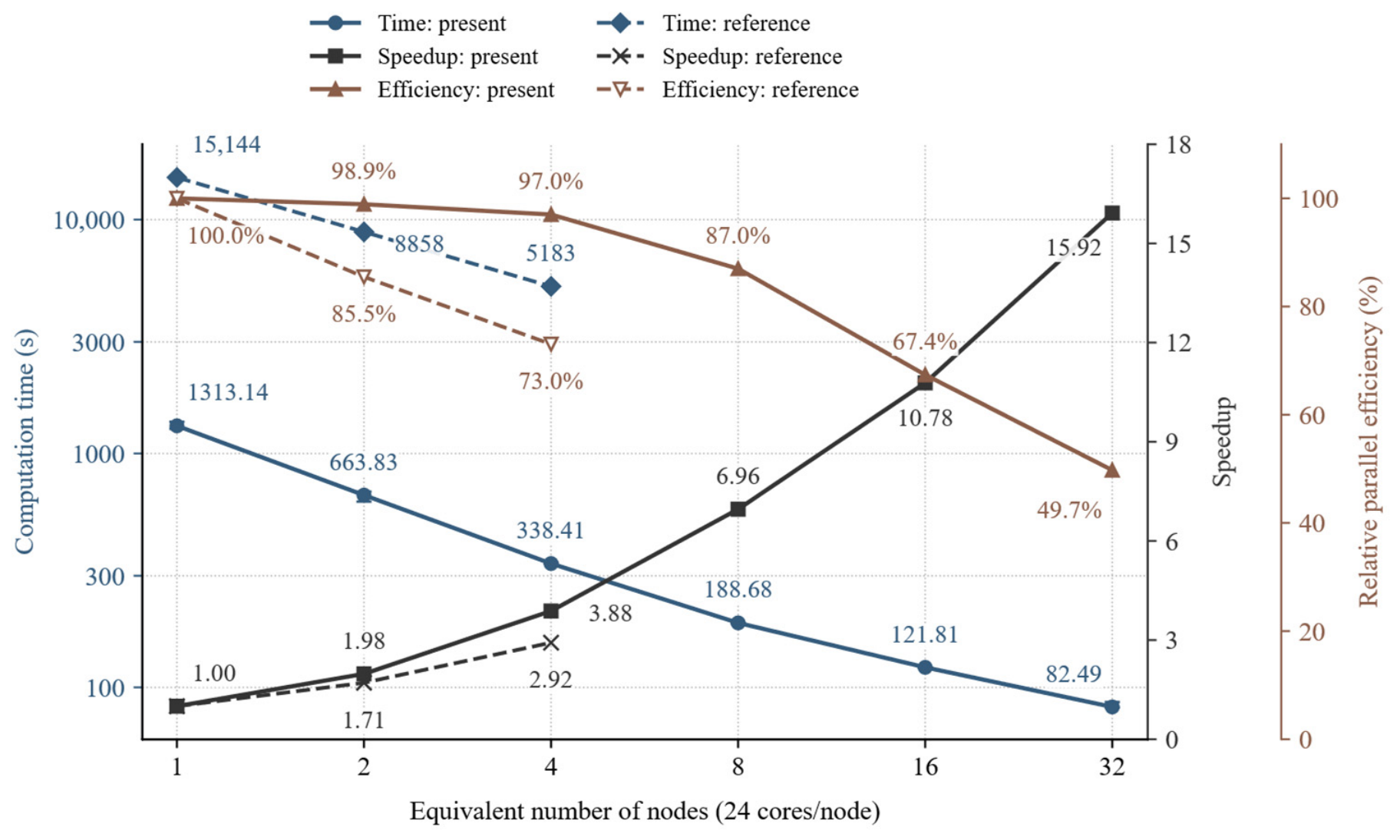
Figure 13 compares the present results with those of Baldan et al. [11], represented by solid and dashed lines, respectively. The horizontal axis expresses core allocations as equivalent node counts based on 24 cores per node, while speedup and relative parallel efficiency are normalized to each study’s own 24-core baseline. The PDPL framework exhibits nearly linear scaling up to four nodes, where the relative parallel efficiency is 97.0%; at eight nodes, the efficiency remains 87.0%. Increasing the allocation from one to 32 nodes reduces the computation time from 1313.14 to 82.49 s, yielding a speedup of 15.92 and an efficiency of 49.7%. Computation time continues to decrease throughout the tested range, although the gains diminish at larger allocations.
Figure 13.
Computation time (s), speedup, and relative parallel efficiency (%) for one million 21 μm droplets on the NACA64A008 horizontal tail. The horizontal axis gives the equivalent number of nodes at 24 cores per node. Speedup and efficiency are normalized to each study’s own 24-core baseline. Solid lines show the present results, and dashed lines show those of Baldan et al. [11].
Baldan et al. [11] use cell tagging and weighted spatial repartitioning to align the allocation of computational resources with the particle workload. However, tracking tasks remain dependent on the particle distribution within each subdomain. Spatial and temporal variations in this distribution can lead to load imbalance and process idle time, while particles crossing subdomain boundaries require interprocess migration. In the PDPL framework, particle tasks are assigned independently of the mesh partition. Each process can access the complete mesh and independently track its assigned particles over their entire trajectories. Processes therefore do not need to wait for particles to enter a particular spatial subdomain or transfer particle states during tracking. For large particle populations, approximately equal numbers of particles can be assigned to each process. As the process count increases, the number of particles handled by each process decreases, supporting more effective use of parallel resources.
The scaling results in Figure 13 illustrate this advantage. Although absolute computation times reflect the combined effects of hardware, numerical methods, and parallel implementation, speedup and relative parallel efficiency describe the scaling of each implementation with respect to its own baseline. Increasing the core count from 24 to 96 gives the PDPL framework a speedup of 3.88 and a relative parallel efficiency of 97.0%, compared with 2.92 and 73.0%, respectively, for the reference method. These results indicate that the PDPL framework achieves better parallel scalability over the compared core-count range.
Table 2 provides the measured times for the main computational phases in the same runs used to report the median computation times. For each release batch, the first seed is located cooperatively by 24 MPI processes within one compute node, and its host–cell identifier is then broadcast to all processes. The remaining particles are localized independently by their assigned processes. Thus, the first-seed search is parallel, but its parallelism does not increase with the total node count. The approximately 30 s reported for this operation is the accumulated search interval over all release batches. At 32 nodes, this interval is 31.25 s, or 37.9% of the total computation time. Meanwhile, the trajectory-integration interval decreases from 1275.61 s on one node to 46.24 s on 32 nodes. The increasing share of seed localization therefore helps explain the departure from linear scaling at larger node counts.
Table 2.
Measured computation time and phase intervals for one million 21 μm droplets.
4. Conclusions
This study presents a Particle-Decomposition Parallel Lagrangian (PDPL) framework for predicting three-dimensional droplet impingement in aircraft-icing simulations. By combining MPI-3 shared-memory windows with particle decomposition, the framework enables node-local data sharing and independent trajectory calculations across compute nodes. The main conclusions drawn from the accuracy assessments and parallel scalability tests are as follows.
- The PDPL framework reduces memory replication through node-local sharing of read-only mesh and background-flow data, while assigning complete trajectories independently of mesh partitioning avoids particle migration both within and across compute nodes. Wall-impact contributions are accumulated locally, with inter-node MPI communication concentrated on their aggregation, thereby reducing communication overhead and improving parallel computational efficiency.
- The framework provides reliable water-collection-efficiency predictions for extruded airfoil sections, curved bluff bodies, the ONERA M6 swept wing, and the NACA64A008 horizontal tail. The principal features of the collection-efficiency distributions and the impingement limits are reproduced well, with good overall agreement with experimental measurements and numerical reference results across the droplet-size conditions considered.
- The million-particle tracking benchmark on the three-dimensional horizontal tail demonstrates that the PDPL framework exhibits good parallel scalability, achieving a parallel efficiency of 97.0% on four nodes and a speedup of 15.92 on 32 nodes, with computation time reduced from 1313.14 s to 82.49 s. At larger node counts, the node-local search for the first seed in each release batch accounts for a growing fraction of the computation time, identifying a specific opportunity for further improvements in scalability.
Author Contributions
Conceptualization, W.X., C.Z. and N.Z.; methodology, W.X. and N.Z.; software, W.X.; validation, W.X.; formal analysis, W.X.; investigation, W.X.; resources, C.Z.; data curation, W.X.; writing—original draft preparation, W.X.; writing—review and editing, W.X., N.Z., C.Z. and C.T.; visualization, W.X.; supervision, C.Z.; project administration, C.Z.; funding acquisition, C.Z. All authors have read and agreed to the published version of the manuscript.
Funding
This research was funded by the National Key Research and Development Program of China (grant number 2024YFB4205600) and the National Major Scientific Research Instrument Development Project (grant number 12227802).
Data Availability Statement
The original contributions presented in this study are included in the article. Further inquiries can be directed to the corresponding author.
Conflicts of Interest
The authors declare no conflict of interest.
References
- Federal Aviation Administration. 14 CFR Part 25, Appendix O—Supercooled Large Drop Icing Conditions; U.S. Department of Transportation, Federal Aviation Administration: Washington, DC, USA, 2014.
- Morency, F.; Beaugendre, H.; Baruzzi, G.S.; Habashi, W.G. FENSAP-ICE: A comprehensive 3D simulation system for in-flight icing. In Proceedings of the 15th AIAA Computational Fluid Dynamics Conference, Anaheim, CA, USA, 11–14 June 2001. [Google Scholar] [CrossRef] [Scilit]
- Norde, E.; van der Weide, E.T.A.; Hoeijmakers, H.W.M. Eulerian method for ice crystal icing. AIAA J. 2018, 56, 222–234. [Google Scholar] [CrossRef] [Scilit]
- Wang, C.; Chang, S.; Wu, H. Lagrangian Approach for Simulating Supercooled Large Droplets’ Impingement Effect. J. Aircr. 2015, 52, 524–537. [Google Scholar] [CrossRef] [Scilit]
- Ren, J.; Yi, X.; Wang, Q. Lagrangian simulation method of droplet collection efficiency for complex configuration. J. Aerosp. Power 2020, 35, 2553–2561. [Google Scholar] [CrossRef]
- Ren, J.; Wang, Q.; Li, W.; Liu, Y.; Yi, X. A prediction algorithm of collection efficiency based on gradient descent method. Acta Aeronaut. Astronaut. Sin. 2023, 44, 126381. [Google Scholar] [CrossRef]
- Han, H.; Yin, Z.; Ning, Y.; Liu, H. Development of a 3D Eulerian/Lagrangian Aircraft Icing Simulation Solver Based on OpenFOAM. Entropy 2022, 24, 1365. [Google Scholar] [CrossRef] [Scilit] [PubMed]
- Rendall, T.C.S.; Allen, C.B. Finite-volume droplet trajectories for icing simulation. Int. J. Multiph. Flow 2014, 58, 185–194. [Google Scholar] [CrossRef] [Scilit]
- Xie, L.; Li, P.; Chen, H.; Liu, H. Robust and efficient prediction of the collection efficiency in icing accretion simulation for 3D complex geometries using the Lagrangian approach I: An adaptive interpolation method based on the restricted radial basis functions. Int. J. Heat Mass Transf. 2020, 150, 119290. [Google Scholar] [CrossRef] [Scilit]
- Liu, Y.; Qu, J.; Yi, X.; Wang, Q. A Monte Carlo Lagrangian Droplet Solver with Backpropagation Neural Network for Aircraft Icing Simulation. Trans. Nanjing Univ. Aeronaut. Astronaut. 2023, 40, 566–577. [Google Scholar] [CrossRef]
- Baldan, G.; Bellosta, T.; Guardone, A. Efficient Lagrangian particle tracking algorithms for distributed-memory architectures. Comput. Fluids 2023, 256, 105856. [Google Scholar] [CrossRef] [Scilit]
- Bellosta, T.; Baldan, G.; Sirianni, G.; Guardone, A. Lagrangian and Eulerian algorithms for water droplets in in-flight icing accretion. J. Comput. Appl. Math. 2023, 429, 115230. [Google Scholar] [CrossRef] [Scilit]
- Zayni, K.; Blanchet, M.; Laurendeau, É. A ray-tracing-enhanced Lagrangian particle tracking framework for ice accretion applications. Aerosp. Sci. Technol. 2026, 175, 112019. [Google Scholar] [CrossRef] [Scilit]
- Clift, R.; Grace, J.R.; Weber, M.E. Bubbles, Drops, and Particles; Academic Press: New York, NY, USA, 1978. [Google Scholar]
- Wright, W.B. Semi-Empirical Modeling of SLD Physics; NASA/TM–2004–212916; National Aeronautics and Space Administration: Cleveland, OH, USA, 2004.
- Mundo, C.; Sommerfeld, M.; Tropea, C. Droplet-wall collisions: Experimental studies of the deformation and breakup process. Int. J. Multiph. Flow 1995, 21, 151–173. [Google Scholar] [CrossRef] [Scilit]
- Papadakis, M.; Hung, K.E.; Vu, G.; Yeong, H.W.; Bidwell, C.S.; Breer, M.D.; Bencic, T.J. Experimental Investigation of Water Droplet Impingement on Airfoils, Finite Wings, and an S-Duct Engine Inlet; NASA/TM–2002–211700; National Aeronautics and Space Administration: Washington, DC, USA, 2002.
- Zeng, T.; Wang, Z.; Xiong, H.; Chen, Y.; Zhou, Z. Research on a fast Lagrangian algorithm for water droplet collection efficiency in complex configurations. J. Aerosp. Power 2025, 40, 20220539. [Google Scholar] [CrossRef]
- Tong, X.L.; Luke, E.A. Eulerian simulations of icing collection efficiency using a singularity diffusion model. In Proceedings of the 43rd AIAA Aerospace Sciences Meeting and Exhibit, Reno, NV, USA, 10–13 January 2005. [Google Scholar] [CrossRef] [Scilit]
- Bidwell, C.S.; Mohler, S.R., Jr. Collection efficiency and ice accretion calculations for a sphere, a swept MS(1)-317 wing, a swept NACA-0012 wing tip, an axisymmetric inlet, and a Boeing 737-300 inlet. In Proceedings of the 33rd Aerospace Sciences Meeting and Exhibit, Reno, NV, USA, 9–12 January 1995. [Google Scholar]
- Sang, W.; Shi, Y.; Xi, C. Numerical simulation of icing effect and ice accretion on three-dimensional configurations. Sci. China Technol. Sci. 2013, 56, 2278–2288. [Google Scholar] [CrossRef] [Scilit]
- Peña, D.; Hoarau, Y.; Laurendeau, E. A single step ice accretion model using Level-Set method. J. Fluids Struct. 2016, 65, 278–294. [Google Scholar] [CrossRef] [Scilit]

Disclaimer/Publisher’s Note: The statements, opinions and data contained in all publications are solely those of the individual author(s) and contributor(s) and not of MDPI and/or the editor(s). MDPI and/or the editor(s) disclaim responsibility for any injury to people or property resulting from any ideas, methods, instructions or products referred to in the content. |
© 2026 by the authors. Licensee MDPI, Basel, Switzerland. This article is an open access article distributed under the terms and conditions of the Creative Commons Attribution (CC BY) license.