Distributed Finite-Time Formation Control for Multi-Parafoil Swarms Under Actuator Saturation Constraints

Abstract

Rapid formation control of multi-parafoil swarms under gust disturbances and steering-line stroke limits is challenging because three-dimensional virtual commands must be realized through only two control channels and post-allocation saturation causes command mismatch. To address these problems, this paper proposes a distributed integral nonsingular fast terminal sliding-mode (INFTSM) controller based on a nonlinear six-degree-of-freedom model under the rigid-composite canopy–payload assumption, with gusts and steering-line saturation explicitly represented. Using information from neighboring parafoils, a controller maps virtual commands to symmetric and asymmetric steering inputs; the saturation residuals, gusts, and bounded modeling uncertainties form a lumped disturbance. An adaptive variable-gain power reaching law (AVPRL) adjusts the reaching gain according to the magnitude of the sliding variable, causing the gain to approach a prescribed minimum near the sliding manifold. Under bounded disturbances and sufficient residual control capability, Lyapunov and homogeneity analyses establish nominal finite-time convergence and local finite-time error bounds. Finally, 200 paired Monte Carlo trials are conducted on a software-in-the-loop (SIL) simulation platform based on MATLAB/Simulink and RflySim. The results show that the proposed method achieves a final 100 s formation-error RMSE of 58.706 ± 31.984 m, a conditional settling time of 629.29 ± 38.16 s, and an actuator saturation percentage of 1.046 ± 0.191%. These results demonstrate that, under the considered simulation conditions, the proposed method achieves multi-parafoil swarm formation control while satisfying the steering-line constraints and provides a favorable overall balance among tracking accuracy, convergence speed, and actuator-constraint handling.

1. Introduction

In large-scale emergency rescue and material delivery scenarios, traditional surface transportation methods are frequently constrained by complex terrains and harsh environments. Unmanned parafoil vehicle (UPV) systems offer long-range unpowered gliding and guided landing capabilities at low-to-medium altitudes, making them relevant to airdrop applications [1]. As the complexity of airdrop missions escalates, the limitations of a single parafoil regarding transport efficiency and fault tolerance become increasingly apparent; consequently, the cooperative airdrop of multi-parafoil swarms has emerged as a research frontier in aerospace engineering [2]. Coordinated multi-parafoil flight may improve payload distribution and system-level fault tolerance.

However, the engineering application of multi-parafoil swarms is subject to multiple dynamic and physical constraints. Once released from the aircraft, a parafoil enters an unpowered gliding descent, and the available altitude limits the time for formation assembly and trajectory tracking [3]. In addition, the flexible canopy–payload system is underactuated, exposed to low-altitude gusts, and constrained by the maximum downward deflection of the trailing-edge steering lines [4]. The interaction between wind disturbances and limited control authority further complicates parafoil homing and trajectory correction [5].

To satisfy the spatiotemporal coordination requirements of swarm flight, distributed formation-control techniques have advanced considerably in recent years. Compared with centralized architectures that rely on global information, methods based on relative states and distributed cooperative mechanisms are commonly used because of their resilience and scalability [6]. In finite-time tracking control, sliding-mode control (SMC) has attracted attention owing to its robustness against matched disturbances [7]. To avoid the singularity of conventional terminal sliding modes near the equilibrium point, nonsingular fast terminal sliding mode (NFTSM) has been applied to multi-agent systems to improve convergence behavior [8]. Reference [9] developed adaptive finite-time compensation control for disturbed UAV swarms, whereas Reference [10] proposed a sliding-mode disturbance-rejection strategy for complex environments. These studies provide a theoretical basis for distributed multi-agent cooperative control, finite-time convergence, and disturbance rejection.

To address input saturation, existing finite-/fixed-time control studies have mainly employed anti-windup and compensation methods [11], auxiliary dynamic systems [12], adaptive saturation compensation [13], command or reference governors, and explicitly constrained optimization [14,15,16]. These methods can effectively handle input constraints under their respective system models and assumptions, but their control structures and saturation-compensation mechanisms generally need to be designed for the specific actuator and control-input configuration. In the parafoil formation-control system studied here, the distributed cooperative-control layer first generates a three-dimensional virtual control command, whereas the physical execution layer has only two independent steering-line channels; actuator saturation therefore occurs after the virtual command has passed through physical control allocation. Accordingly, the closed-loop system is subject not only to direct input-amplitude limits but also to the mapping discrepancy between the virtual control quantity and the physical actuation, as well as the command-truncation error caused by actuator saturation. Unlike methods that introduce additional compensator states or an online constrained-optimization layer, this study represents the post-allocation saturation-truncation error as a bounded dynamic residual and incorporates it, together with gust disturbances and bounded modeling uncertainties, into a unified closed-loop robustness analysis. The reaching-law term is used to limit the influence of this residual under the stated boundedness condition, making the resulting control framework compatible with the parafoil’s two-channel, stroke-limited actuation architecture.

In summary, existing studies have made important advances in distributed formation control, finite-/fixed-time convergence, robust sliding-mode control, and input-saturation treatment, providing an important theoretical foundation for distributed cooperative control of multi-agent systems. Nevertheless, for parafoil swarms characterized by unpowered descent, underactuation, and steering-line stroke constraints, challenges remain in the physical realization of control commands and the convergence of cooperative errors under nonideal conditions.

First, some existing distributed formation-control methods are based on simplified dynamic models or formulate cooperative-control laws at the virtual-control level, focusing primarily on formation-error convergence, finite-time stability, and disturbance rejection [6,7,8,9,10]. These methods generally assume that the virtual control commands can be realized by the low-level actuators. However, the parafoil system considered in this study exhibits nonlinear 6-DOF dynamics and can produce control action only through two steering-line channels corresponding to symmetric and asymmetric deflections. Owing to this underactuation, the three-dimensional virtual cooperative-control command generated by the cooperative controller cannot be applied directly to the physical parafoil; it must be converted into physically realizable steering-line inputs through a control-allocation mechanism. Therefore, the focus of this study is not to redesign the consensus mechanism but to provide a physically implementable mapping from the virtual cooperative-control layer to the parafoil execution layer under the stated actuation constraints.

Second, existing studies have addressed input saturation using anti-windup and compensation methods, auxiliary dynamic systems, adaptive saturation compensation, command governors, and explicitly constrained optimization [11,12,13,14,15,16]. These approaches can effectively handle input constraints under their respective system models and assumptions, but their control structures and saturation-compensation mechanisms are generally designed for systems in which the control inputs act directly on the actuators. In the parafoil-swarm system studied here, the cooperative-control layer first generates a three-dimensional virtual command, which must be converted into actual steering-line inputs through underactuated control allocation. Actuator saturation therefore occurs during the mapping from the virtual control quantity to the physical actuation. The resulting error includes not only the truncation error caused by steering-line stroke limits but also the mismatch between the actual post-allocation actuation capability and the desired control action. Consequently, another key problem in parafoil-swarm control is how to incorporate the post-allocation saturation residual, gust disturbances, and model uncertainties into a unified closed-loop robustness analysis without introducing an additional complex compensation structure. This treatment assumes that the actuator saturation residual, external disturbances, and model uncertainties are bounded and that the system retains sufficient control authority under saturation. If the desired control demand persistently exceeds the physically attainable control range of the parafoil, the associated finite-time convergence result no longer applies.

To address these problems, based on a nonlinear 6-DOF equivalent-rigid-body dynamic model of the parafoil under the rigid-composite canopy–payload assumption, this paper proposes an integral nonsingular fast terminal sliding mode (INFTSM) cooperative-control strategy tailored to an underactuated parafoil platform subject to actuator saturation constraints. A parafoil-specific control-allocation mechanism maps the three-dimensional virtual cooperative-control command into symmetric and asymmetric steering-line inputs. The command-truncation error caused by actuator saturation during control allocation is incorporated, together with gust disturbances and bounded modeling uncertainties, into a lumped disturbance term. Meanwhile, an adaptive variable-gain power reaching law (AVPRL) adjusts the reaching gain according to the sliding variable, applying a larger gain for larger cooperative errors and approaching a prescribed minimum near the sliding manifold. Under the stated assumptions, Lyapunov and homogeneity analyses establish nominal finite-time convergence and a local practical finite-time bound for bounded residual disturbances. The main contributions are summarized as follows:

• A physically constrained nonlinear 6-DOF equivalent-rigid-body model of the multi-parafoil system is established. Under the rigid-composite canopy–payload assumption, the model incorporates composite inertial properties, aerodynamic moment-arm effects, translational–rotational coupling, gust disturbances, and steering-line stroke constraints, providing a dynamic basis for distributed formation control.
• A graph-based INFTSM cooperative-control framework accounting for underactuation and actuator saturation is developed. Neighbor-based cooperative errors are used to construct the virtual commands, which are mapped into symmetric and asymmetric steering-line inputs; the post-allocation residual is then included with gusts and bounded modeling uncertainties in the robustness analysis.
• An adaptive variable-gain power reaching law (AVPRL) is designed to regulate the reaching gain according to the sliding-variable magnitude. The gain increases with the sliding-variable magnitude and approaches a prescribed minimum near the sliding manifold. Lyapunov and homogeneity analyses establish nominal finite-time convergence and a local practical finite-time bound under the stated disturbance and control-authority conditions.

The remainder of this paper is organized as follows: Section 2 establishes the 6-DOF dynamic model of a single parafoil and presents the distributed communication topology and error definitions, incorporating physical constraints. Section 3 elaborates on the design process of the proposed graph-based INFTSM cooperative controller and the AVPRL. Section 4 provides the robust stability proof for both the reaching and sliding phases based on Lyapunov’s theory. Section 5 conducts software-in-the-loop (SIL) comparative simulations and quantitative analyses using the RflySim-based simulation platform. Finally, Section 6 concludes the paper.

2. Modeling and Problem Description

2.1. Parafoil Modeling and Coordinate System Definition

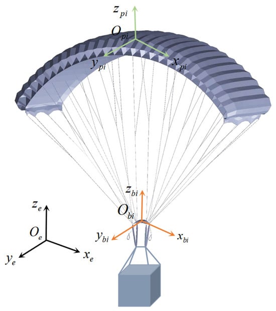
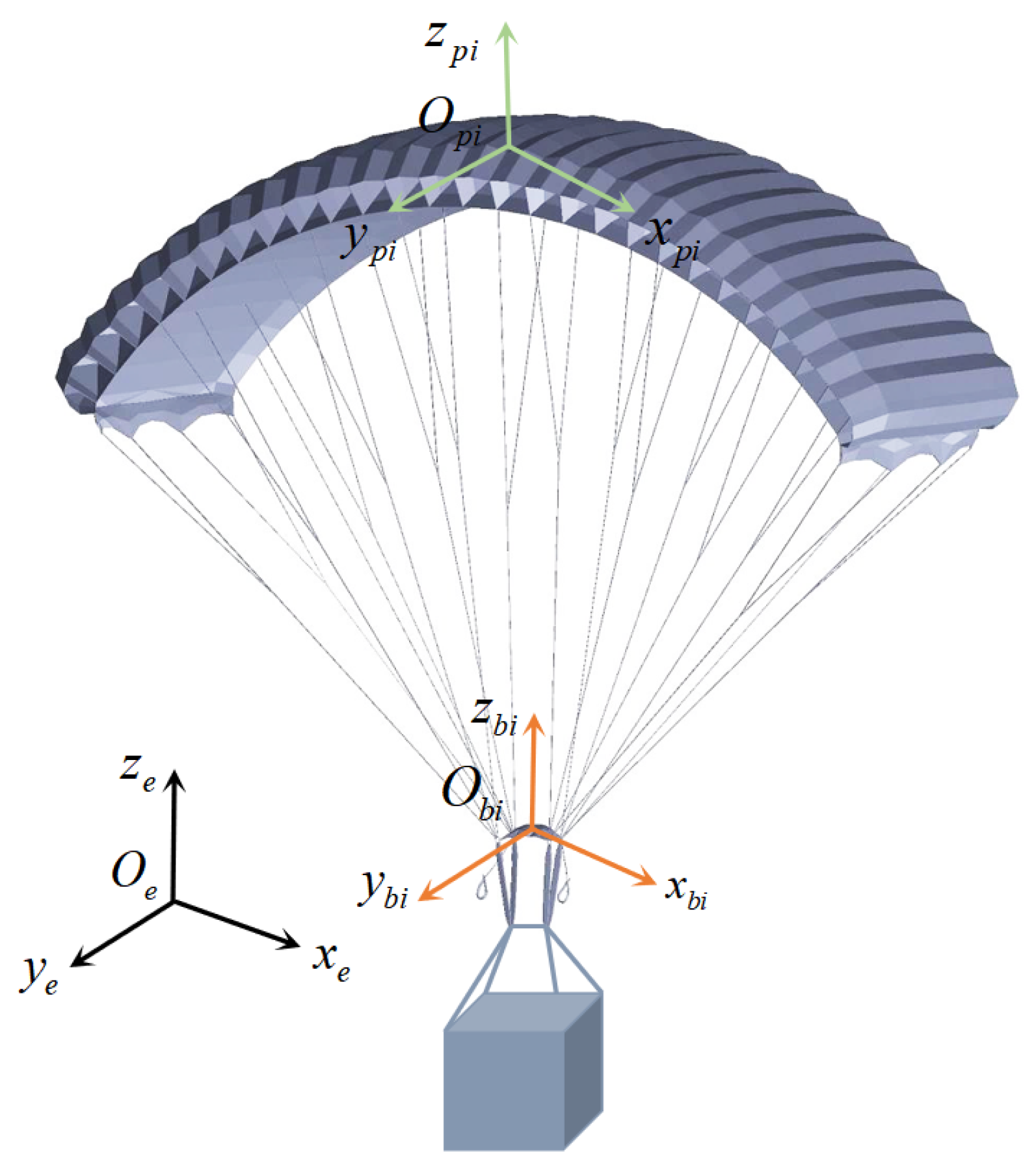
A parafoil system primarily consists of a flexible canopy that maintains its airfoil shape through internal inflation, suspension lines, steering lines, and a payload at the bottom. To accurately describe the spatial position and attitude motion of the parafoil system, the reference coordinate frames are established as shown in Figure 1 [17,18,19,20]. The spatial kinematic model employs three coordinate frames. Within the spatial and temporal scope of the multi-parafoil swarm airdrop mission, neglecting the effects of Earth’s curvature and rotation, a local Earth-fixed inertial frame ${\mathcal{F}}_e=\{O_e,x_e,y_e,z_e\}$ is established, with its axes pointing north, west, and upward, respectively. The body-fixed frame of the i-th parafoil, ${\mathcal{F}}_{b_i}=\{O_{b_i},x_{b_i},y_{b_i},z_{b_i}\}$, has its origin at the center of mass of the rigid composite system, with its axes pointing forward, left, and upward. Under zero-attitude conditions, its axes align with the corresponding axes of the inertial frame. The canopy-fixed frame, ${\mathcal{F}}_{p_i}=\{O_{p_i},x_{p_i},y_{p_i},z_{p_i}\}$, has its origin at the nominal aerodynamic center of the canopy. These definitions follow coordinate and modeling conventions used in parafoil trajectory-planning and 6-DOF studies [21,22,23,24,25].

Figure 1. Structure of the unmanned parafoil system. The black, orange, and green arrows represent the coordinate axes of the Earth-fixed inertial frame ${\mathcal{F}}_e$, body-fixed frame ${\mathcal{F}}_{b_i}$, and canopy-fixed frame ${\mathcal{F}}_{p_i}$, respectively.

To balance modeling accuracy and the computational efficiency of the multi-agent swarm algorithm, this paper neglects the relative degrees of freedom caused by flexible deformation and canopy–payload pendular motion. The relative pose of ${\mathcal{F}}_{p_i}$ with respect to ${\mathcal{F}}_{b_i}$ is assumed to remain constant, and the position vector from $O_{b_i}$ to $O_{p_i}$, expressed in ${\mathcal{F}}_{b_i}$, is denoted by the constant vector ${\mathit{r}}_{b_i{p}_i}^{b_i}$. The corresponding axes of ${\mathcal{F}}_{p_i}$ and ${\mathcal{F}}_{b_i}$ are chosen to be mutually parallel; therefore, the constant transformation matrix between the two frames is ${\mathit{R}}_{p_i}^{b_i}={\mathit{I}}_3$. Accordingly, the model is formulated as a nonlinear 6-DOF equivalent-rigid-body model under the rigid-composite canopy–payload assumption.

The position of the body-frame origin in the inertial frame is denoted by ${\mathit{P}}_i={\left[\begin{array}{ccc}{x}_i& y_i& z_i\end{array}\right]}^{\mathrm{T}}$. The attitude of the system is described using the 3–2–1 yaw–pitch–roll Euler-angle convention, defined as ${\mathbf{\Theta }}_i={\left[\begin{array}{ccc}{\phi }_i& {\theta }_i& {\psi }_i\end{array}\right]}^{\mathrm{T}}$, where ${\phi }_i$, ${\theta }_i$, and ${\psi }_i$ denote the roll, pitch, and yaw angles, respectively. The direction-cosine matrix ${\mathit{R}}_{b_i}^e\left({\mathbf{\Theta }}_i\right)$, which maps a vector from the body frame ${\mathcal{F}}_{b_i}$ to the inertial frame ${\mathcal{F}}_e$, is

$${\mathit{R}}_{b_i}^e\left({\mathbf{\Theta }}_i\right)=\left[\begin{array}{ccc}\cos {\theta }_i\cos {\psi }_i& \sin {\phi }_i\sin {\theta }_i\cos {\psi }_i-\cos {\phi }_i\sin {\psi }_i& \cos {\phi }_i\sin {\theta }_i\cos {\psi }_i+\sin {\phi }_i\sin {\psi }_i\\ \cos {\theta }_i\sin {\psi }_i& \sin {\phi }_i\sin {\theta }_i\sin {\psi }_i+\cos {\phi }_i\cos {\psi }_i& \cos {\phi }_i\sin {\theta }_i\sin {\psi }_i-\sin {\phi }_i\cos {\psi }_i\\ -\sin {\theta }_i& \sin {\phi }_i\cos {\theta }_i& \cos {\phi }_i\cos {\theta }_i\end{array}\right].$$

(1)

The aerodynamic loads of the system are initially calculated in the canopy frame ${\mathcal{F}}_{p_i}$. According to the rigid-body wrench-transport relation, these loads are mapped to the equivalent force and moment about the center of mass $O_{b_i}$, resolved in the body frame ${\mathcal{F}}_{b_i}$, as follows:

$${\mathit{F}}_{\mathrm{aero},i}^{b_i}={\mathit{R}}_{p_i}^{b_i}{\mathit{F}}_{\mathrm{aero},i}^{p_i},$$

(2)

$${\mathit{M}}_{\mathrm{aero},O_{b_i},i}^{b_i}={\mathit{R}}_{p_i}^{b_i}{\mathit{M}}_{\mathrm{aero},O_{p_i},i}^{p_i}+{\mathit{r}}_{b_i{p}_i}^{b_i}\times {\mathit{F}}_{\mathrm{aero},i}^{b_i}.$$

(3)

To avoid notational clutter in subsequent equations, let ${\mathit{F}}_{\mathrm{aero},i}\equiv {\mathit{F}}_{\mathrm{aero},i}^{b_i}$ and ${\mathit{M}}_{\mathrm{aero},i}\equiv {\mathit{M}}_{\mathrm{aero},O_{b_i},i}^{b_i}$. Thus, the moment-arm effect caused by the offset of the aerodynamic center relative to the center of mass, ${\mathit{r}}_{b_i{p}_i}^{b_i}\times {\mathit{F}}_{\mathrm{aero},i}^{b_i}$, is incorporated into the equivalent aerodynamic moment ${\mathit{M}}_{\mathrm{aero},i}$ and is not part of the mass or inertia matrices.

Based on the equivalent rigid-body assumption and the aerodynamic-load transformation above, the translational and rotational dynamics of the i-th parafoil, resolved in ${\mathcal{F}}_{b_i}$, are

$${\dot{\mathit{V}}}_i={\mathit{M}}_{\mathrm{sys}}^{-1}\left({\mathit{F}}_{\mathrm{aero},i}({\delta }_{s,i}^{\mathrm{act}},{\delta }_{a,i}^{\mathrm{act}})+{\mathit{F}}_{g,i}+{\mathit{d}}_{F,i}-{\mathit{\omega }}_i\times \left({\mathit{M}}_{\mathrm{sys}}{\mathit{V}}_i\right)\right),$$

(4)

$${\dot{\mathit{\omega }}}_i={\mathit{I}}_{\mathrm{sys}}^{-1}\left({\mathit{M}}_{\mathrm{aero},i}({\delta }_{s,i}^{\mathrm{act}},{\delta }_{a,i}^{\mathrm{act}})+{\mathit{d}}_{M,i}-{\mathit{\omega }}_i\times \left({\mathit{I}}_{\mathrm{sys}}{\mathit{\omega }}_i\right)\right).$$

(5)

For clarity, the aerodynamic quantities entering Equations (4) and (5) are parameterized in the canopy frame as

$$q_{\infty ,i}=\frac{1}{2}\rho V_{a,i}^2,{\mathit{F}}_{\mathrm{aero},i}^{p_i}=q_{\infty ,i}{S}_p{\mathit{C}}_F({\alpha }_i,{\beta }_i,{\delta }_{s,i}^{\mathrm{act}},{\delta }_{a,i}^{\mathrm{act}}),$$

(6)

$${\mathit{M}}_{\mathrm{aero},O_{p_i},i}^{p_i}=q_{\infty ,i}{S}_p\mathrm{diag}(b,\overline{c},b){\mathit{C}}_M({\alpha }_i,{\beta }_i,{\delta }_{s,i}^{\mathrm{act}},{\delta }_{a,i}^{\mathrm{act}}),$$

(7)

where $V_{a,i}$ is the airspeed relative to the local wind, $\rho$ is air density, $S_p$, b, and $\overline{c}$ are the canopy reference area, span, and chord, respectively, and ${\alpha }_i$ and ${\beta }_i$ are the angle of attack and sideslip angle. The fixed coefficient maps ${\mathit{C}}_F={[C_X,C_Y,C_Z]}^{\mathrm{T}}$ and ${\mathit{C}}_M={[C_l,C_m,C_n]}^{\mathrm{T}}$ include the steering-effectiveness derivatives and are used by the 6-DOF plant; they are not inverted by the allocator, which instead uses measured kinematic variables and the calibrated gains in Section 3.4. Here, ${\mathit{V}}_i={\left[\begin{array}{ccc}{u}_i& v_i& w_i\end{array}\right]}^{\mathrm{T}}$ and ${\mathit{\omega }}_i={\left[\begin{array}{ccc}{p}_i& q_i& r_i\end{array}\right]}^{\mathrm{T}}$ are the linear and angular velocity vectors in the body frame, respectively. The generalized mass matrix ${\mathit{M}}_{\mathrm{sys}}\in {\mathbb{R}}^{3\times 3}$ comprises the physical- and apparent-mass contributions, whereas the generalized inertia matrix ${\mathit{I}}_{\mathrm{sys}}\in {\mathbb{R}}^{3\times 3}$ comprises the combined-system inertia, the contributions obtained from the parallel-axis theorem, and the apparent moment of inertia. Since the $z_e$ axis points vertically upward, the gravitational force resolved in the body frame is ${\mathit{F}}_{g,i}={\mathit{R}}_e^{b_i}\left({\mathbf{\Theta }}_i\right){\left[\begin{array}{ccc}0& 0& -m_{\mathrm{sys}}g\end{array}\right]}^{\mathrm{T}}$, where ${\mathit{R}}_e^{b_i}\left({\mathbf{\Theta }}_i\right)={\left[{\mathit{R}}_{b_i}^e\left({\mathbf{\Theta }}_i\right)\right]}^{-1}={\left[{\mathit{R}}_{b_i}^e\left({\mathbf{\Theta }}_i\right)\right]}^{\mathrm{T}}$ and $m_{\mathrm{sys}}$ is the total physical mass.

The aerodynamic force ${\mathit{F}}_{\mathrm{aero},i}$ and aerodynamic moment ${\mathit{M}}_{\mathrm{aero},i}$ are driven by the actual trailing-edge deflections. The two inputs obey the coupled steering-line constraint ${\delta }_{s,i}^{\mathrm{act}}\ge 0$ and ${\delta }_{s,i}^{\mathrm{act}}+\left|{\delta }_{a,i}^{\mathrm{act}}\right|\le \kappa$, where $\kappa$ is the maximum steering-line deflection used by the plant. The unknown disturbances caused by low-altitude wind gusts and aerodynamic-parameter perturbations are characterized by ${\mathit{d}}_{F,i}$ and ${\mathit{d}}_{M,i}$.

A complete 12-dimensional state vector is defined as ${\mathit{x}}_i={\left[\begin{array}{cccc}{\mathit{P}}_i^{\mathrm{T}}& {\mathbf{\Theta }}_i^{\mathrm{T}}& {\mathit{V}}_i^{\mathrm{T}}& {\mathit{\omega }}_i^{\mathrm{T}}\end{array}\right]}^{\mathrm{T}}$. For $\cos {\theta }_i\ne 0$, the transformation matrix that maps the body angular velocity to the Euler-angle rates is

$${\mathit{T}}_{\mathrm{\Theta }}\left({\mathbf{\Theta }}_i\right)=\left[\begin{array}{ccc}1& \sin {\phi }_i\tan {\theta }_i& \cos {\phi }_i\tan {\theta }_i\\ 0& \cos {\phi }_i& -\sin {\phi }_i\\ 0& {\displaystyle \frac{\sin {\phi }_i}{\cos {\theta }_i}}& {\displaystyle \frac{\cos {\phi }_i}{\cos {\theta }_i}}\end{array}\right].$$

(8)

Furthermore, the derivative of the direction-cosine matrix satisfies

$${\dot{\mathit{R}}}_{b_i}^e\left({\mathbf{\Theta }}_i\right)={\mathit{R}}_{b_i}^e\left({\mathbf{\Theta }}_i\right){\left[{\mathit{\omega }}_i\right]}_{\times },{\left[{\mathit{\omega }}_i\right]}_{\times }=\left[\begin{array}{ccc}0& -r_i& q_i\\ r_i& 0& -p_i\\ -q_i& p_i& 0\end{array}\right].$$

(9)

Here, ${\mathit{T}}_{\mathrm{\Theta }}\left({\mathbf{\Theta }}_i\right)$ represents the attitude-kinematic transformation. Accordingly, the position and attitude kinematics are given by Equations (10) and (11):

$${\dot{\mathit{P}}}_i={\mathit{R}}_{b_i}^e\left({\mathbf{\Theta }}_i\right){\mathit{V}}_i,$$

(10)

$${\dot{\mathbf{\Theta }}}_i={\mathit{T}}_{\mathrm{\Theta }}\left({\mathbf{\Theta }}_i\right){\mathit{\omega }}_i.$$

(11)

Under the rigid-composite canopy–payload assumption and the block-diagonal approximation of the translational–rotational apparent-mass matrix, this nonlinear 6-DOF equivalent-rigid-body model retains the principal rigid-body nonlinear terms and practical actuation constraints, providing a consistent dynamic basis for the subsequent design of the finite-time sliding-mode controller.

2.2. Distributed Communication Topology and Error Dynamic Modeling

In multi-parafoil swarm airdrop missions, genuinely distributed cooperation requires each follower parafoil to construct its control law using only its own state and the state information received from local communication neighbors, without relying on global absolute coordinates or network-wide broadcasts from the leader.

2.2.1. Graph Theory Description of Communication Topology

This paper adopts a graph-based cooperative-control framework, arranging the swarm into a triangular formation through predefined relative-position offsets. The connectivity of this topology provides the basis for constructing the neighbor-dependent errors and for the subsequent stability analysis.

In this paper, the communication topology among the follower parafoils is abstracted as an undirected graph $\mathcal{G}=(\mathcal{V},\mathcal{E},\mathit{A})$, where $\mathcal{V}=\{1,2,\dots ,N\}$ is the follower-index set, $\mathcal{E}\subseteq \mathcal{V}\times \mathcal{V}$ is the undirected edge set, and $\mathit{A}=\left[a_{ij}\right]$ is the weighted adjacency matrix. If parafoil i can receive information from parafoil j, then $a_{ij}>0$; otherwise, $a_{ij}=0$. The undirected topology satisfies $a_{ij}=a_{ji}$. The degree of node i is $\mathrm{deg}\left(i\right)={\sum }_{j=1}^N{a}_{ij}$, and the degree matrix is $\mathit{D}=\mathrm{diag}\{\mathrm{deg}\left(1\right),\dots ,\mathrm{deg}\left(N\right)\}\in {\mathbb{R}}^{N\times N}$. Consequently, the Laplacian matrix is $\mathit{L}=\mathit{D}-\mathit{A}$. When the second-smallest eigenvalue of $\mathit{L}$ satisfies ${\lambda }_2>0$, the graph $\mathcal{G}$ is connected, meaning that a communication path exists between any two nodes.

Furthermore, the leader-augmented graph is denoted by $\overline{\mathcal{G}}$. It consists of one leader parafoil and N follower parafoils. The coupling matrix between the leader and the followers is $\mathit{C}=\mathrm{diag}\{c_1,c_2,\dots ,c_N\}\in {\mathbb{R}}^{N\times N}$. If the i-th follower receives information from the leader, then $c_i>0$; otherwise, $c_i=0$.

Assumption 1. 

In the augmented communication graph $\overline{\mathcal{G}}$, there exists at least one path from the leader to every follower parafoil (i.e., the augmented graph contains a spanning tree rooted at the leader). Under this assumption, $\mathit{H}=\mathit{L}+\mathit{C}$ is symmetric positive definite, providing the graph-theoretic basis for convergence of the distributed errors.

Assumption 2 (Communication condition).

During the formation maneuver considered in this study, the communication topology is fixed, and each follower has access to the current states of its communication neighbors and the leader if directly connected. The leader-acceleration feedforward term ${\mathit{U}}_0$ required by Equation (36) is assumed to be available at the cooperative-control layer. If reconstructed from sampled leader states, its estimation error is assumed to be bounded and included in the lumped disturbance considered in Section 4.2. Communication delays, packet losses, and asynchronous sampling are neglected, i.e., ${\tau }_{ij}=0$ for all active communication links.

Under these assumptions, the distributed errors in Equations (12) and (13) are constructed from synchronous state information. Accordingly, the subsequent stability and finite-time convergence results apply to a fixed-topology, delay-free, packet-loss-free, and synchronously sampled communication setting.

2.2.2. Distributed Consensus Tracking Error Definition

Let the inertial-frame position and velocity of the leader parafoil be ${\mathit{P}}_0$ and ${\mathit{V}}_{e,0}$, respectively. The swarm is expected to form a predefined spatial configuration. Let ${\mathit{d}}_i\in {\mathbb{R}}^3$ denote the desired spatial offset of the i-th follower relative to the leader. Consequently, the desired relative displacement between followers i and j is ${\mathit{d}}_{ij}={\mathit{d}}_i-{\mathit{d}}_j$. Based on local-neighbor information, the distributed position and velocity cooperative errors, ${\mathit{E}}_{p,i}$ and ${\mathit{E}}_{v,i}$, are defined by Equations (12) and (13), respectively:

$${\mathit{E}}_{p,i}=\sum _{j\in {\mathcal{N}}_i}{a}_{ij}\left(\left({\mathit{P}}_i-{\mathit{P}}_j\right)-{\mathit{d}}_{ij}\right)+c_i\left({\mathit{P}}_i-{\mathit{P}}_0-{\mathit{d}}_i\right),$$

(12)

$${\mathit{E}}_{v,i}=\sum _{j\in {\mathcal{N}}_i}{a}_{ij}\left({\mathit{V}}_{e,i}-{\mathit{V}}_{e,j}\right)+c_i\left({\mathit{V}}_{e,i}-{\mathit{V}}_{e,0}\right).$$

(13)

Here, ${\mathcal{N}}_i$ is the neighbor set of the i-th parafoil, and $a_{ij}$ is the topological weight ($a_{ij}>0$ if parafoil i can receive information from parafoil j). The term $c_i$ represents the leader observation weight ($c_i>0$ only if parafoil i can communicate directly with the leader; otherwise, $c_i=0$), and ${\mathit{V}}_{e,i}={\mathit{R}}_{b_i}^e\left({\mathbf{\Theta }}_i\right){\mathit{V}}_i$ is the inertial-frame linear velocity of the i-th parafoil. For the fixed and delay-free communication topology considered here, ${\mathcal{N}}_i$, $a_{ij}$, and $c_i$ are time invariant, and all relative-state terms in Equations (12) and (13) are evaluated using synchronous state information at time t. The leader velocity is ${\mathit{V}}_{e,0}={\dot{\mathit{P}}}_0$, and the prescribed offsets ${\mathit{d}}_i$ (and hence ${\mathit{d}}_{ij}$) are constant in the inertial frame. These definitions imply the kinematic identity ${\dot{\mathit{E}}}_{p,i}={\mathit{E}}_{v,i}$ used in the subsequent stability analysis.

2.2.3. Control Objective and Physical Constraints

Combining the single-parafoil 6-DOF model with the communication topology, the control objective is to design the deflection commands ${\delta }_{s,i}^{cmd}$ and ${\delta }_{a,i}^{cmd}$ such that, in the nominal case, the distributed cooperative errors reach and remain at the origin after a finite time. Under bounded disturbances and actuator saturation, a local disturbance-dependent practical bound is sought under the conditions stated in Section 4:

$${\mathit{E}}_{p,i}\left(t\right)={\mathbf{0}}_3,{\mathit{E}}_{v,i}\left(t\right)={\mathbf{0}}_3,\forall t\ge T_i,\exists T_i<\infty ,\forall i\in \{1,2,\dots ,N\}.$$

(14)

Furthermore, since the matrix $\mathit{H}=\mathit{L}+\mathit{C}$ is positive definite, the convergence of the local cooperative error ${\mathit{E}}_{p,i}$ is mathematically equivalent to the corresponding convergence of the absolute formation-tracking error ${\tilde{\mathit{P}}}_i={\mathit{P}}_i-{\mathit{P}}_0-{\mathit{d}}_i$.

3. Distributed Finite-Time Controller Design

Based on the 6-DOF dynamic model and the distributed communication topology established in Section 2, this section details the design process of the finite-time cooperative controller for the multi-parafoil swarm. To address formation tracking under gust disturbances and steering-line constraints, the control derivation in this section follows a progressive logic:

• First, the guidance strategy of the leader parafoil is designed to generate a smooth reference baseline that satisfies dynamic feasibility for the swarm (Section 3.1).
• Second, incorporating local neighborhood interaction information, a distributed error dynamic model considering physical constraints is constructed (Section 3.2).
• Third, an INFTSM surface is designed based on local interaction information (Section 3.3).
• Finally, an adaptive variable-gain power reaching law is designed, from which the actual physical control commands of each individual parafoil are resolved (Section 3.4).

3.1. Leader Trajectory Tracking and Guidance Control

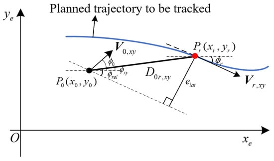
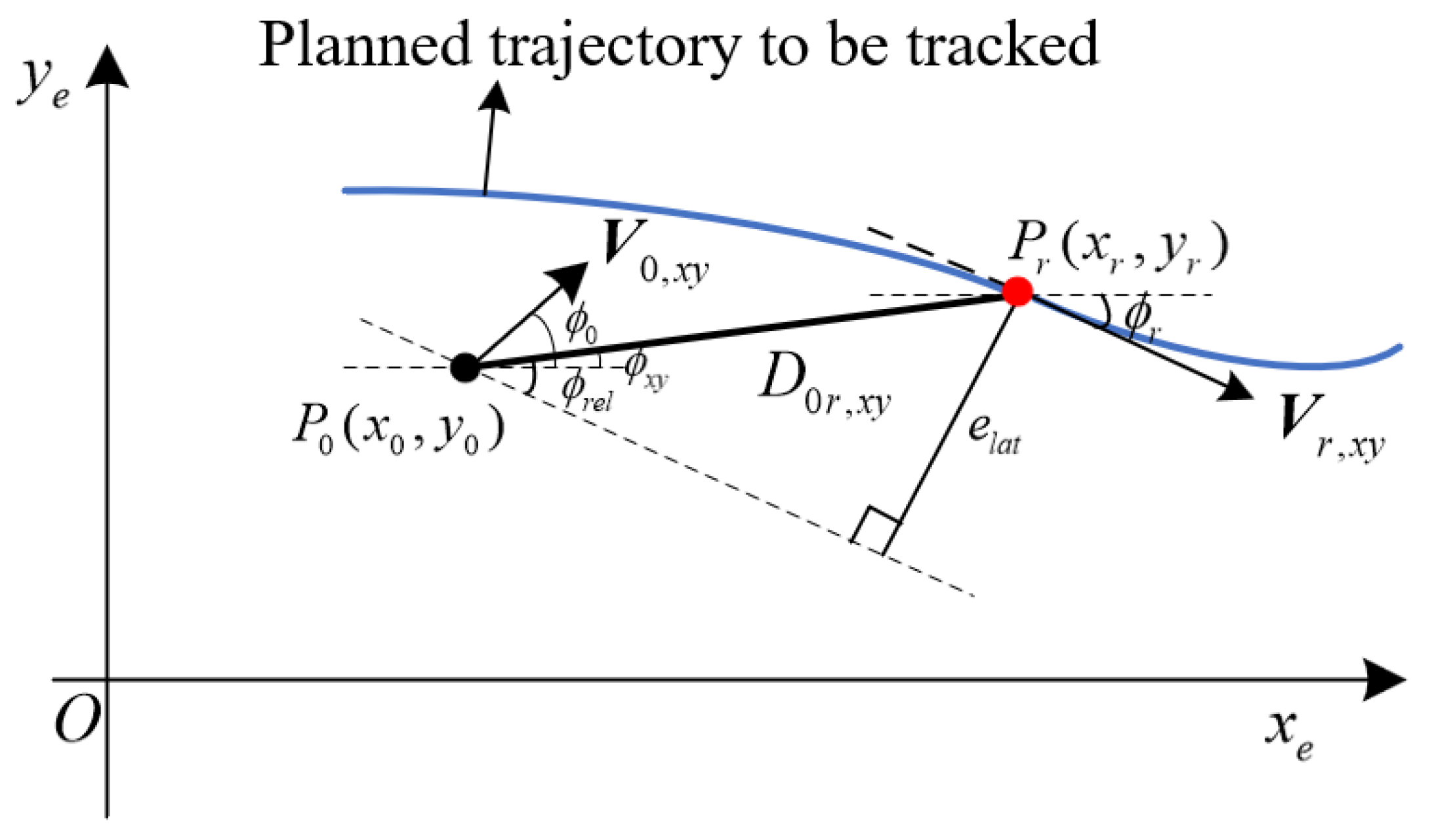
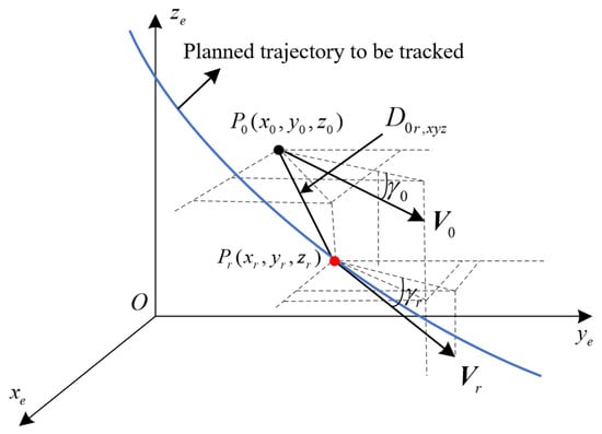
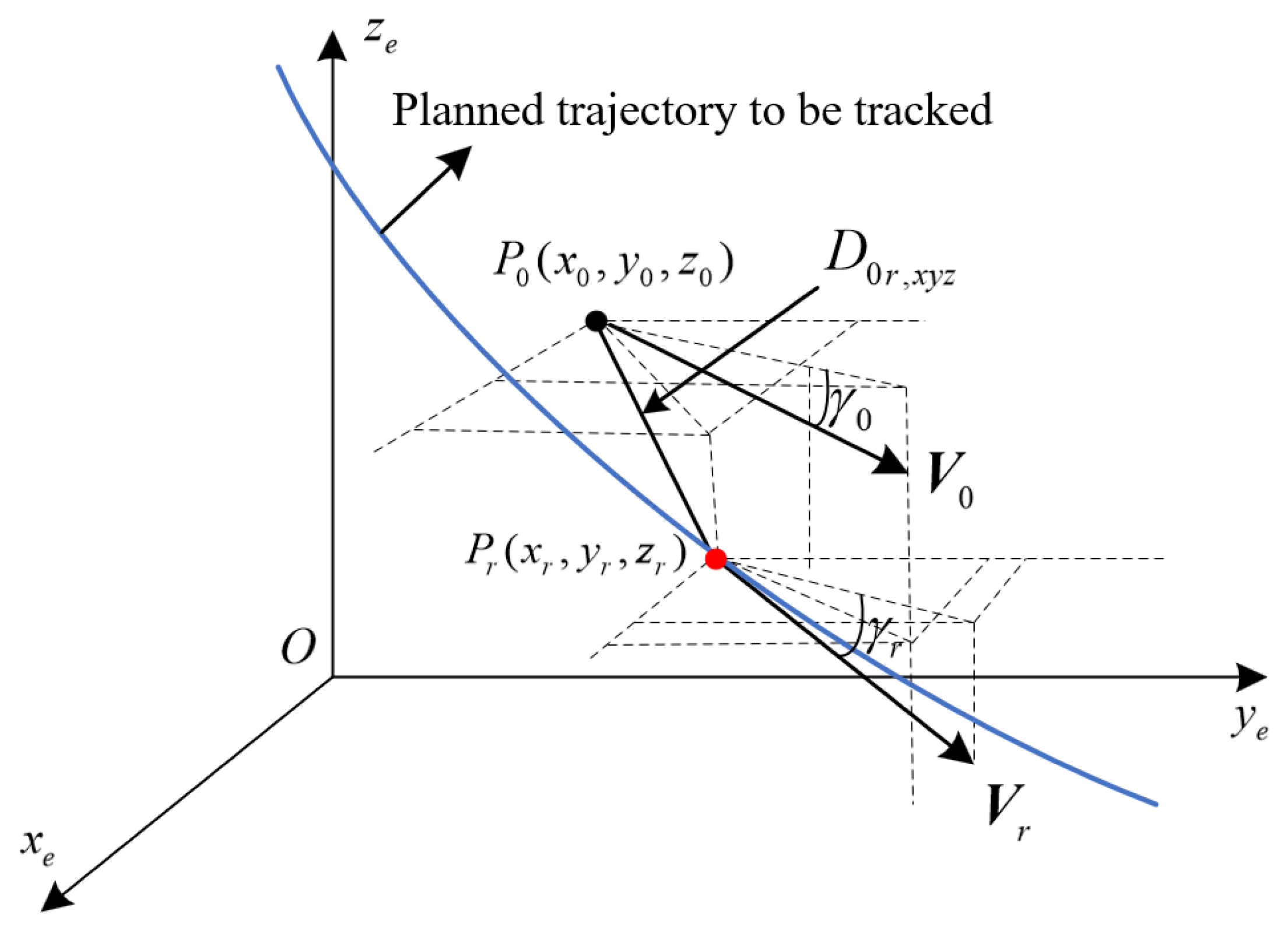
In the distributed formation topology, the leader parafoil provides the reference trajectory for the followers. Its local controller employs a Stanley-type guidance strategy to generate the commanded speed $V_c$, heading angle ${\varphi }_c$, and flight-path angle ${\gamma }_c$ from the lateral and longitudinal geometric deviations. The guidance command vector is defined as ${\mathit{q}}_c={\left[\begin{array}{ccc}{V}_c& {\varphi }_c& {\gamma }_c\end{array}\right]}^{\mathrm{T}}$. The resulting leader states ${\mathit{P}}_0$ and ${\mathit{V}}_{e,0}$ are transmitted to the pinned followers through the coupling weights $c_i$. In Figure 2 and Figure 3, the shorter label ${\mathit{V}}_0\equiv {\mathit{V}}_{e,0}$ is used for readability. The symbols $\varphi$ and $\gamma$ are retained in this leader-guidance subsection, whereas $\chi$ and $\mu$ in Section 3.4 denote the corresponding ground-track heading and flight-path angle used by the follower allocation loop.

Figure 2. Lateral trajectory tracking of the leader parafoil. The red dot denotes the current reference point $P_r(x_r,y_r)$ on the planned trajectory.

Figure 3. Longitudinal trajectory tracking of the leader parafoil. The red dot denotes the current reference point $P_r(x_r,y_r,z_r)$ on the planned trajectory.

3.1.1. Velocity Command Decomposition

The scalar speed command $V_c$ and the commanded angles in ${\mathit{q}}_c$ define the inertial-frame velocity command ${\mathit{V}}_c^e={\left[\begin{array}{ccc}{V}_{c,x}& V_{c,y}& V_{c,z}\end{array}\right]}^{\mathrm{T}}$ as follows:

$$\left\{\begin{array}{c}{V}_{c,x}=V_c\cos \left({\varphi }_c\right)\cos \left({\gamma }_c\right),\hfill \\ V_{c,y}=V_c\sin \left({\varphi }_c\right)\cos \left({\gamma }_c\right),\hfill \\ V_{c,z}=V_c\sin \left({\gamma }_c\right).\hfill \end{array}\right.$$

(15)

Here, $V_c$ is typically set to the equilibrium gliding velocity of the parafoil.

3.1.2. Lateral Guidance Law Design

According to Figure 2, the lateral Euclidean distance $D_{0r,xy}$ between the current position of the leader parafoil $(x_0,y_0)$ and the reference trajectory point $(x_r,y_r)$ is defined as

$$D_{0r,xy}=\sqrt{{(x_0-x_r)}^2+{(y_0-y_r)}^2}.$$

(16)

The angle ${\varphi }_{xy}$ represents the angle between $D_{0r,xy}$ and the x-axis, which can be obtained through the following formula:

$${\varphi }_{xy}=\mathrm{atan}2(y_r-y_0,x_r-x_0),$$

(17)

where $\mathrm{atan}2(·,·)$ is the four-quadrant inverse tangent function. The leader’s ground-track heading is ${\varphi }_0=\mathrm{atan}2(V_{0,y},V_{0,x})$, where $V_{0,x}$ and $V_{0,y}$ are components of ${\mathit{V}}_0$. Thus, ${\varphi }_0$ is distinct from the roll angle ${\phi }_0$ and the attitude yaw angle ${\psi }_0$. The tangent heading of the reference path is

$${\varphi }_r=\mathrm{atan}2\left({\dot{y}}_r,{\dot{x}}_r\right),$$

(18)

where ${\dot{x}}_r$ and ${\dot{y}}_r$ are the horizontal velocity components of the reference trajectory at the current reference point. The heading angle error $e_{\varphi }$ is obtained by subtracting the current heading angle ${\varphi }_0$ from the desired heading angle ${\varphi }_r$. To handle periodic angle jumps, the following normalization process is applied:

$$e_{\varphi }=\left\{\begin{array}{cc}{\varphi }_r-{\varphi }_0-2\pi ,\hfill & {\varphi }_r-{\varphi }_0>\pi ,\hfill \\ {\varphi }_r-{\varphi }_0+2\pi ,\hfill & {\varphi }_r-{\varphi }_0<-\pi ,\hfill \\ {\varphi }_r-{\varphi }_0,\hfill & \mathrm{otherwise}.\hfill \end{array}\right.$$

(19)

Furthermore, based on the geometric relationship illustrated in Figure 2, the lateral deviation $e_{\mathrm{lat}}$ of the leader parafoil can be derived as

$$e_{\mathrm{lat}}=D_{0r,xy}\sin \left({\varphi }_{\mathrm{rel}}\right),$$

(20)

where ${\varphi }_{\mathrm{rel}}$ is the relative angle shown in Figure 2. Consequently, the Stanley-type heading control law calculates the heading command for the next guidance update:

$${\varphi }_c={\varphi }_0+{\dot{\varphi }}_{\mathrm{corr}}\Delta t,$$

(21)

$${\dot{\varphi }}_{\mathrm{corr}}=k_{\mathrm{lat},1}{e}_{\mathrm{lat}}+k_{\mathrm{lat},2}{e}_{\varphi },$$

(22)

where ${\dot{\varphi }}_{\mathrm{corr}}$ is the heading-correction rate, $k_{\mathrm{lat},1},k_{\mathrm{lat},2}>0$ are its feedback gains, and $\Delta t$ is the guidance update interval.

3.1.3. Altitude (Longitudinal) Guidance Law Design

Similarly, according to Figure 3, the spatial distance $D_{0r,xyz}$ in the longitudinal plane is defined as

$$D_{0r,xyz}=\sqrt{{(x_0-x_r)}^2+{(y_0-y_r)}^2+{(z_0-z_r)}^2}.$$

(23)

The angles ${\gamma }_r$ and ${\gamma }_0=\arcsin (V_{0,z}/{\parallel {\mathit{V}}_0\parallel }_2)$ are the reference and actual flight-path angles, respectively; ${\gamma }_0$ is distinct from the pitch angle ${\theta }_0$. Based on the reference-path kinematics,

$${\gamma }_r=\arcsin \left({\displaystyle \frac{{\dot{z}}_r}{V_r}}\right),$$

(24)

where ${\mathit{V}}_r={\left[\begin{array}{ccc}{\dot{x}}_r& {\dot{y}}_r& {\dot{z}}_r\end{array}\right]}^{\mathrm{T}}$ is the reference-path velocity vector and $V_r={\parallel {\mathit{V}}_r\parallel }_2$ is its speed. The raw flight-path-angle difference ${\gamma }_r-{\gamma }_0$ is normalized to $[-\pi ,\pi ]$ as follows:

$$e_{\gamma }=\left\{\begin{array}{cc}{\gamma }_r-{\gamma }_0-2\pi ,\hfill & {\gamma }_r-{\gamma }_0>\pi ,\hfill \\ {\gamma }_r-{\gamma }_0+2\pi ,\hfill & {\gamma }_r-{\gamma }_0<-\pi ,\hfill \\ {\gamma }_r-{\gamma }_0,\hfill & \mathrm{otherwise}.\hfill \end{array}\right.$$

(25)

Based on the ideal reference glide path angle, the longitudinal altitude deviation $e_{\mathrm{lon}}$ is defined as

$$e_{\mathrm{lon}}=(z_r-z_0)-D_{0r,xyz}\sin \left({\gamma }_0\right).$$

(26)

The Stanley-type flight-path-angle control law is constructed as follows:

$${\gamma }_c={\gamma }_0+{\dot{\gamma }}_{\mathrm{corr}}\Delta t,$$

(27)

$${\dot{\gamma }}_{\mathrm{corr}}=k_{\mathrm{lon},1}{e}_{\mathrm{lon}}+k_{\mathrm{lon},2}{e}_{\gamma },$$

(28)

where ${\dot{\gamma }}_{\mathrm{corr}}$ is the flight-path correction rate and $k_{\mathrm{lon},1},k_{\mathrm{lon},2}>0$ are its feedback gains.

In summary, the real-time state of the leader parafoil, generated by the aforementioned lateral and longitudinal guidance laws, provides a unified reference position and velocity baseline for all follower parafoils within the swarm. The subsequent graph-based cooperative controller uses this baseline to reduce the follower formation-tracking errors within the considered airdrop scenario.

It is important to distinguish the role of the leader-guidance law from that of the subsequent INFTSM–AVPRL cooperative controller. Geometric or vector-field guidance methods primarily construct a desired heading, flight-path angle, or velocity direction from path-geometry errors. Their advantages include an intuitive structure and relatively low computational cost, which make them well suited to single-vehicle reference-path tracking. However, a guidance field by itself does not generally establish a finite-time convergence result for multi-agent formation errors, nor does it necessarily account explicitly for command truncation caused by finite steering-line strokes. In the present architecture, the Stanley-type law is therefore used only to generate the reference motion of the leader parafoil, whereas formation assembly and consensus tracking of the followers are governed by the INFTSM–AVPRL cooperative controller. The two components are complementary rather than interchangeable: the guidance law generates the reference trajectory, while the proposed controller addresses cooperative-error convergence and physical command realization.

Compared with conventional vector-field guidance and asymptotic formation-control approaches, the proposed cooperative-control layer has three relevant features. First, the integral nonsingular fast terminal sliding surface employs non-Lipschitz error feedback to establish nominal finite-time convergence and a local practical finite-time bound under the stated bounded-residual conditions. The AVPRL applies a larger reaching gain when the sliding variable is far from the manifold and smoothly reduces the gain near the manifold. Second, wind gusts and bounded modeling uncertainties are incorporated into the closed-loop lumped disturbance, so their bounded influence is included in the stability analysis rather than considered only through numerical testing. Third, the three-dimensional virtual cooperative command is mapped through the underactuated control-allocation mechanism to the physically available symmetric and asymmetric steering-line inputs. The finite stroke is imposed through explicit clipping, and the resulting command–execution mismatch is retained as a bounded residual in the robustness analysis. Thus, the proposed scheme complements geometric guidance with a cooperative-control layer that considers finite-time convergence, bounded gust disturbances, and actuator saturation in the underactuated parafoil model.

3.2. Distributed Error Dynamics Considering 6-DOF Physical Constraints

Based on the previously defined distributed position and velocity cooperative errors ${\mathit{E}}_{p,i}$ and ${\mathit{E}}_{v,i}$, their relation to the body-frame 6-DOF model requires the derivative of the inertial-frame velocity ${\mathit{V}}_{e,i}={\mathit{R}}_{b_i}^e\left({\mathbf{\Theta }}_i\right){\mathit{V}}_i$:

$${\dot{\mathit{V}}}_{e,i}={\mathit{R}}_{b_i}^e\left({\mathbf{\Theta }}_i\right){\dot{\mathit{V}}}_i+{\dot{\mathit{R}}}_{b_i}^e\left({\mathbf{\Theta }}_i\right){\mathit{V}}_i.$$

(29)

Substituting the 6-DOF translational dynamics into the above relation yields the inertial-frame acceleration of the i-th parafoil:

$$\begin{array}{cc}\hfill {\dot{\mathit{V}}}_{e,i}=& {\mathit{R}}_{b_i}^e\left({\mathbf{\Theta }}_i\right)\left[{\mathit{M}}_{\mathrm{sys}}^{-1}\left({\mathit{F}}_{\mathrm{aero},i}({\delta }_{s,i}^{\mathrm{act}},{\delta }_{a,i}^{\mathrm{act}})+{\mathit{F}}_{g,i}+{\mathit{d}}_{F,i}-{\mathit{\omega }}_i\times \left({\mathit{M}}_{\mathrm{sys}}{\mathit{V}}_i\right)\right)\right]+{\dot{\mathit{R}}}_{b_i}^e\left({\mathbf{\Theta }}_i\right){\mathit{V}}_i.\hfill \end{array}$$

(30)

Furthermore, differentiating ${\mathit{E}}_{v,i}$ gives the distributed error dynamics:

$${\dot{\mathit{E}}}_{v,i}=\sum _{j\in {\mathcal{N}}_i}{a}_{ij}({\dot{\mathit{V}}}_{e,i}-{\dot{\mathit{V}}}_{e,j})+c_i({\dot{\mathit{V}}}_{e,i}-{\dot{\mathit{V}}}_{e,0}).$$

(31)

In this nonlinear model, the aerodynamic force is constrained by the steering-line stroke. Local-neighbor information is used to construct the cooperative errors, and the fixed-topology cooperative-control layer maps the stacked errors into ${\delta }_{s,i}^{\mathrm{cmd}}$ and ${\delta }_{a,i}^{\mathrm{cmd}}$, which are subsequently clipped to obtain the actual inputs.

3.3. Integral Nonsingular Fast Terminal Sliding-Mode Surface Based on Local Neighborhood Information

For finite-time convergence analysis without the singular terms associated with conventional terminal sliding modes near the equilibrium, the following integral nonsingular fast terminal sliding-mode surface is designed for the i-th follower parafoil based on local interaction information:

$${\mathit{s}}_i={\mathit{E}}_{v,i}+{\int }_0^t\left[{\mathbf{\Lambda }}_1{\mathit{E}}_{v,i}\left(\tau \right)+{\mathbf{\Lambda }}_2{\mathrm{sig}}^{\alpha }\left({\mathit{E}}_{v,i}\left(\tau \right)\right)+{\mathbf{\Lambda }}_3{\mathrm{sig}}^{\beta }\left({\mathit{E}}_{p,i}\left(\tau \right)\right)\right]\mathrm{d}\tau .$$

(32)

Here, ${\mathit{s}}_i\in {\mathbb{R}}^3$ and ${\mathbf{\Lambda }}_{\mathit{\ell }}\in {\mathbb{R}}^{3\times 3}$, $\mathit{\ell }\in \{1,2,3\}$, are positive-definite diagonal gain matrices; $\alpha \in (0,1)$, and $\beta =\alpha /(2-\alpha )$. The unsubscripted $\alpha$ and $\beta$ in the controller denote sliding-surface exponents and are distinct from the aerodynamic angles ${\alpha }_i$ and ${\beta }_i$ in Section 2.1. For $\mathit{x}={\left[\begin{array}{ccc}{x}_1& x_2& x_3\end{array}\right]}^{\mathrm{T}}\in {\mathbb{R}}^3$, the signum-power mapping is defined componentwise for $\chi >0$ as

$${\mathrm{sig}}^{\chi }\left(\mathit{x}\right)={\left[\begin{array}{ccc}|x_1{|}^{\chi }\mathrm{sgn}\left(x_1\right)& |x_2{|}^{\chi }\mathrm{sgn}\left(x_2\right)& |x_3{|}^{\chi }\mathrm{sgn}\left(x_3\right)\end{array}\right]}^{\mathrm{T}}.$$

(33)

The effects of command realization, steering-line clipping, gusts, and modeling uncertainty are represented by the lumped bounded disturbance defined in Section 4.2.

3.4. Variable-Gain Cooperative Reaching Law and Actuator Mapping

To vary the reaching gain with the sliding-variable magnitude, this paper introduces the following AVPRL:

$${\dot{\mathit{s}}}_i=-k_a{\mathit{s}}_i-k_b\left({\mathit{s}}_i\right){\mathrm{sig}}^{\chi }\left({\mathit{s}}_i\right),$$

(34)

where $k_a>0$ and $0<\chi <1$. Unlike conventional constant gains, the switching gain $k_b\left({\mathit{s}}_i\right)$ is designed as a nonlinear function of the Euclidean norm ${\parallel {\mathit{s}}_i\parallel }_2$:

$$k_b\left({\mathit{s}}_i\right)=k_{\min }+(k_{\max }-k_{\min })\left[1-\exp \left(-\mu {\parallel {\mathit{s}}_i\parallel }_2\right)\right],$$

(35)

where $k_{\max }>k_{\min }>0$ represent the upper and lower bounds of the gain, respectively, and $\mu >0$ is the regulation rate coefficient. When the system is far from the sliding surface (${\parallel {\mathit{s}}_i\parallel }_2$ is large), the dynamic gain $k_b\left({\mathit{s}}_i\right)\to k_{\max }$; when the system approaches the sliding surface (${\parallel {\mathit{s}}_i\parallel }_2\to 0$), the gain smoothly approaches $k_{\min }$, reducing the control activity near the surface.

Let ${\mathit{U}}_F=\mathrm{col}({\dot{\mathit{V}}}_{e,1},\dots ,{\dot{\mathit{V}}}_{e,N})$. Stacking Equation (31) gives ${\dot{\mathit{E}}}_v=(\mathit{H}\otimes {\mathit{I}}_3){\mathit{U}}_F-(\mathit{C}{\mathbf{1}}_N\otimes {\mathit{I}}_3){\mathit{U}}_0$. By differentiating the sliding surface and combining this relation with the AVPRL, the stacked raw equivalent-acceleration command is obtained as

$$\begin{array}{cc}\hfill {\mathit{U}}_F^{\mathrm{raw}}& =\left({\mathit{H}}^{-1}\otimes {\mathit{I}}_3\right)\left[\left(\mathit{C}{\mathbf{1}}_N\otimes {\mathit{I}}_3\right){\mathit{U}}_0-{\mathit{F}}_s-k_a\mathit{S}-{\mathit{K}}_b\left(\mathit{S}\right){\mathrm{sig}}^{\chi }\left(\mathit{S}\right)\right],\hfill \\ \hfill {\mathit{F}}_s& =\left({\mathit{I}}_N\otimes {\mathbf{\Lambda }}_1\right){\mathit{E}}_v+\left({\mathit{I}}_N\otimes {\mathbf{\Lambda }}_2\right){\mathrm{sig}}^{\alpha }\left({\mathit{E}}_v\right)+\left({\mathit{I}}_N\otimes {\mathbf{\Lambda }}_3\right){\mathrm{sig}}^{\beta }\left({\mathit{E}}_p\right),\hfill \\ \hfill {\mathit{K}}_b\left(\mathit{S}\right)& =\mathrm{diag}\left\{k_b\left({\mathit{s}}_1\right){\mathit{I}}_3,\dots ,k_b\left({\mathit{s}}_N\right){\mathit{I}}_3\right\}.\hfill \end{array}$$

(36)

Here, $\mathrm{col}(·)$ stacks its arguments into a column, ${\mathbf{1}}_N$ is the N-dimensional vector of ones, ${\mathit{U}}_F^{\mathrm{raw}}=\mathrm{col}({\mathit{U}}_{F,1}^{\mathrm{raw}},\dots ,{\mathit{U}}_{F,N}^{\mathrm{raw}})$, ${\mathit{U}}_0={\dot{\mathit{V}}}_{e,0}$, $\mathit{S}=\mathrm{col}({\mathit{s}}_1,\dots ,{\mathit{s}}_N)$, ${\mathit{E}}_p=\mathrm{col}({\mathit{E}}_{p,1},\dots ,{\mathit{E}}_{p,N})$, and ${\mathit{E}}_v=\mathrm{col}({\mathit{E}}_{v,1},\dots ,{\mathit{E}}_{v,N})$. Although the cooperative errors are neighbor based, the direct multiplication by ${\mathit{H}}^{-1}$ in Equation (36) is a network-level algebraic operation. In the present fixed-topology SIL implementation, ${\mathit{H}}^{-1}$ is precomputed and the stacked command is evaluated in the cooperative-control layer. A fully decentralized onboard realization would require an equivalent distributed linear solver or estimator, which is outside the present scope.

Since the generated acceleration command may exceed the physical capability of the parafoil system, the command for follower i is constrained as

$${\mathit{U}}_{\mathrm{eq},i}={\mathrm{\Pi }}_{{\mathrm{\Omega }}_a}\left({\mathit{U}}_{F,i}^{\mathrm{raw}}\right),$$

(37)

where ${\mathrm{\Omega }}_a=\{\mathit{u}\in {\mathbb{R}}^3:{\parallel \mathit{u}\parallel }_2\le a_{\max }\}$, $a_{\max }=2.5\mathrm{m}/{\mathrm{s}}^2$, and ${\mathrm{\Pi }}_{{\mathrm{\Omega }}_a}(·)$ denotes the Euclidean projection onto ${\mathrm{\Omega }}_a$. The resulting ${\mathit{U}}_{\mathrm{eq},i}$ is a three-dimensional virtual acceleration command in the inertial frame rather than a directly realizable actuator input.

The parafoil system possesses six degrees of freedom but only two independent control inputs, namely the symmetric and asymmetric steering-line deflections ${\delta }_{s,i}^{\mathrm{act}}$ and ${\delta }_{a,i}^{\mathrm{act}}$. Therefore, the mapping ${\mathit{U}}_{\mathrm{eq},i}\mapsto ({\delta }_{s,i}^{\mathrm{cmd}},{\delta }_{a,i}^{\mathrm{cmd}})$ cannot be obtained through conventional full-state dynamic inversion. The adopted hierarchy converts ${\mathit{U}}_{\mathrm{eq},i}$ into a feasible velocity command, forms speed and flight-direction errors, generates longitudinal and lateral control contributions, and maps them to normalized left- and right-line demands. These demands are clipped to obtain admissible line variables and then reconstructed into the physically applied steering deflections.

3.4.1. Virtual Acceleration Transformation

The virtual acceleration command is converted into a desired velocity vector using the previous feasible command:

$$\left\{\begin{array}{cc}\hfill {\mathit{v}}_{c,i}^{\mathrm{raw}}\left[k\right]& ={\mathit{v}}_{c,i}[k-1]+T_c{\mathit{U}}_{\mathrm{eq},i}\left[k\right],T_c=0.1\mathrm{s},\hfill \\ \hfill {\mathit{v}}_{c,i}[k-1]& ={\left[\begin{array}{ccc}{V}_{c,i}\cos {\mu }_{c,i}\cos {\chi }_{c,i}& V_{c,i}\cos {\mu }_{c,i}\sin {\chi }_{c,i}& V_{c,i}\sin {\mu }_{c,i}\end{array}\right]}_{k-1}^{\mathrm{T}}.\hfill \end{array}\right.$$

(38)

Writing ${\mathit{v}}_{c,i}^{\mathrm{raw}}={[v_{x,c,i}^{\mathrm{raw}},v_{y,c,i}^{\mathrm{raw}},v_{z,c,i}^{\mathrm{raw}}]}^{\mathrm{T}}$, the raw velocity vector is converted into the commanded speed, flight-path angle, and heading angle as

$$\left\{\begin{array}{cc}\hfill V_{c,i}^{\mathrm{raw}}& =\sqrt{{\left(v_{x,c,i}^{\mathrm{raw}}\right)}^2+{\left(v_{y,c,i}^{\mathrm{raw}}\right)}^2+{\left(v_{z,c,i}^{\mathrm{raw}}\right)}^2},\hfill \\ \hfill {\mu }_{c,i}^{\mathrm{raw}}& ={\sin }^{-1}\left({\displaystyle \frac{v_{z,c,i}^{\mathrm{raw}}}{V_{c,i}^{\mathrm{raw}}}}\right),\hfill \\ \hfill {\chi }_{c,i}^{\mathrm{raw}}& =\mathrm{atan}2\left(v_{y,c,i}^{\mathrm{raw}},v_{x,c,i}^{\mathrm{raw}}\right).\hfill \end{array}\right.$$

(39)

Here, the positive $z_e$ axis and positive flight-path angle point upward, consistently with the inertial-frame convention defined in Section 2.1.

3.4.2. Feasible Command and Inner-Loop Regulation

The raw commands are subjected to both envelope and rate limits. For $x\in \{V,\mu \}$,

$$x_{c,i}\left[k\right]=\mathrm{sat}\left(x_{c,i}^{\mathrm{raw}}\left[k\right],\left[\max \{x_{\min },x_{c,i}[k-1]-{\dot{x}}_{\max }{T}_c\},\min \{x_{\max },x_{c,i}[k-1]+{\dot{x}}_{\max }{T}_c\}\right]\right),$$

(40)

and the wrapped heading update is

$${\chi }_{c,i}\left[k\right]={\mathrm{wrap}}_{[-\pi ,\pi )}\left({\chi }_{c,i}[k-1]+\mathrm{sat}\left(\mathbf{\Delta }{\chi }_{c,i}^{\mathrm{raw}},[-{\dot{\chi }}_{\max }{T}_c,{\dot{\chi }}_{\max }{T}_c]\right)\right),$$

(41)

where $\Delta {\chi }_{c,i}^{\mathrm{raw}}={\mathrm{wrap}}_{[-\pi ,\pi )}({\chi }_{c,i}^{\mathrm{raw}}\left[k\right]-{\chi }_{c,i}[k-1])$, ${\mathrm{wrap}}_{[a,b)}(·)$ maps an angle to the indicated interval, and $\mathrm{sat}(x,[a,b\left]\right)=\min \{b,\max \{a,x\left\}\right\}$. The operating envelope and command-rate bounds used in this study are

$$\begin{array}{c}7.9\le V_{c,i}\le 11\mathrm{m}/\mathrm{s},-{25}^{\circ }\le {\mu }_{c,i}\le 8^{\circ },-\pi \le {\chi }_{c,i}<\pi ,\\ |{\dot{V}}_{c,i}|\le 0.5\mathrm{m}/{\mathrm{s}}^2,|{\dot{\mu }}_{c,i}|\le 0.22\mathrm{rad}/\mathrm{s},|{\dot{\chi }}_{c,i}|\le 0.178\mathrm{rad}/\mathrm{s}.\end{array}$$

(42)

Angular calculations in Equations (40) and (41) are performed in radians; degree values in Equation (42) are reported only for readability.

Let ${\mathit{V}}_{e,i}={[V_{x,i},V_{y,i},V_{z,i}]}^{\mathrm{T}}$. The measured speed and flight-direction angles are $V_i={\parallel {\mathit{V}}_{e,i}\parallel }_2$, ${\mu }_i={\sin }^{-1}(V_{z,i}/V_i)$, and ${\chi }_i=\mathrm{atan}2(V_{y,i},V_{x,i})$. To make the calibrated inner-loop gains unambiguous, the angular errors and body rates used below are expressed in degrees:

$$\begin{array}{cc}\hfill e_{V,i}& =V_i-V_{c,i},\hfill \\ \hfill e_{\mu ,i}^{\circ }& ={\displaystyle \frac{180}{\pi }}({\mu }_{c,i}-{\mu }_i),\hfill \\ \hfill e_{\chi ,i}^{\circ }& ={\mathrm{wrap}}_{[-{180}^{\circ },{180}^{\circ })}\left({\displaystyle \frac{180}{\pi }}({\chi }_{c,i}-{\chi }_i)\right),\hfill \end{array}$$

(43)

with $p_i^{\circ }=180p_i/\pi$ and $q_i^{\circ }=180q_i/\pi$. The anti-windup integral states are updated as

$$\begin{array}{cc}\hfill I_{V,i}[k+1]& =\mathrm{sat}(I_{V,i}\left[k\right]+e_{V,i}\left[k\right]T_c,[-2.5,2.5]),\hfill \\ \hfill I_{\mu ,i}[k+1]& =\mathrm{sat}(I_{\mu ,i}\left[k\right]+e_{\mu ,i}^{\circ }\left[k\right]T_c,[-5,5]),\hfill \\ \hfill I_{\chi ,i}[k+1]& =\mathrm{sat}(I_{\chi ,i}\left[k\right]+e_{\chi ,i}^{\circ }\left[k\right]T_c,[-100,100]).\hfill \end{array}$$

(44)

Accordingly, $I_{V,i}$ has units of meters, whereas $I_{\mu ,i}$ and $I_{\chi ,i}$ have units of degree-seconds. The numerical gains below carry the corresponding reciprocal units so that $b_{V,i}$, $b_{\mu ,i}$, and $b_{\chi ,i}$ are dimensionless. The dimensionless longitudinal and lateral control contributions are then

$$\begin{array}{cc}\hfill b_{V,i}& =0.1e_{V,i}+0.2I_{V,i}+0.01q_i^{\circ },\hfill \\ \hfill {\xi }_{\mu ,i}& =20e_{\mu ,i}^{\circ }+15I_{\mu ,i}-30q_i^{\circ },b_{\mu ,i}=-0.2\tanh ({\xi }_{\mu ,i}/100),\hfill \\ \hfill b_{\chi ,i}& ={\displaystyle \frac{\pi }{180}}\left(0.8e_{\chi ,i}^{\circ }+0.06I_{\chi ,i}-0.8p_i^{\circ }\right).\hfill \end{array}$$

(45)

3.4.3. Steering-Line Allocation and Infeasible-Command Handling

This allocation assumes a feasible initialization, quasi-steady steering effectiveness within Equation (42), available measurements of $(V_i,{\mu }_i,{\chi }_i,p_i,q_i)$, and actuator dynamics faster than the outer loop. It is a calibrated hierarchical allocation, not aerodynamic dynamic inversion: no control-effectiveness matrix or pseudoinverse is evaluated online, and the aerodynamic parameters in Equations (6) and (7) enter only through the plant response.

Define $b_{c,i}=b_{V,i}+b_{\mu ,i}$. The unconstrained normalized left- and right-line demands and their admissible values are

$$\begin{array}{cccc}\hfill {\overline{\sigma }}_{L,i}& =0.5+b_{c,i}+b_{\chi ,i},\hfill & \hfill {\sigma }_{L,i}& =\mathrm{sat}({\overline{\sigma }}_{L,i},[0,1]),\hfill \\ \hfill {\overline{\sigma }}_{R,i}& =0.5+b_{c,i},\hfill & \hfill {\sigma }_{R,i}& =\mathrm{sat}({\overline{\sigma }}_{R,i},[0,1]).\hfill \end{array}$$

(46)

The commanded and physically applied steering deflections are reconstructed from the unconstrained and clipped line variables, respectively:

$$\begin{array}{cc}\hfill \left[\begin{array}{c}{\delta }_{a,i}^{\mathrm{cmd}}\\ {\delta }_{s,i}^{\mathrm{cmd}}\end{array}\right]& =\kappa \left[\begin{array}{c}{\overline{\sigma }}_{L,i}-{\overline{\sigma }}_{R,i}\\ \min \{{\overline{\sigma }}_{L,i},{\overline{\sigma }}_{R,i}\}\end{array}\right],\hfill \\ \hfill \left[\begin{array}{c}{\delta }_{a,i}^{\mathrm{act}}\\ {\delta }_{s,i}^{\mathrm{act}}\end{array}\right]& =\kappa \left[\begin{array}{c}{\sigma }_{L,i}-{\sigma }_{R,i}\\ \min \{{\sigma }_{L,i},{\sigma }_{R,i}\}\end{array}\right].\hfill \end{array}$$

(47)

Here, $\kappa =1.5$ is the maximum normalized steering-line deflection scale used by the plant. Because ${\sigma }_{L,i},{\sigma }_{R,i}\in [0,1]$, Equation (47) guarantees

$${\delta }_{s,i}^{\mathrm{act}}\ge 0,{\delta }_{s,i}^{\mathrm{act}}+\left|{\delta }_{a,i}^{\mathrm{act}}\right|=\kappa \max \{{\sigma }_{L,i},{\sigma }_{R,i}\}\le \kappa .$$

(48)

Thus, infeasible requests are treated successively by acceleration projection, flight-envelope/rate limiting, and normalized line clipping; no singular inversion is attempted. Moreover, a feasible previous command gives $V_{c,i}^{\mathrm{raw}}\ge 7.9-a_{\max }{T}_c=7.65\mathrm{m}/\mathrm{s}>0$, so the speed–angle transformation is nonsingular over the stated operating range. The resulting actual deflections are applied to Equations (4) and (5).

4. Stability Analysis

This section analyzes the convergence properties of the INFTSM cooperative controller under wind disturbances and actuator saturation constraints. The Lyapunov analysis is divided into the reaching and sliding phases and states the conditions under which the nominal and practical finite-time conclusions apply.

4.1. Preliminaries and Lemmas

Lemma 1 

(Finite-time stability [26]). Consider the system $\dot{\mathit{x}}=\mathit{f}\left(\mathit{x}\right)$. If there exists a continuous positive-definite Lyapunov function $\mathcal{V}\left(\mathit{x}\right)$ satisfying

$$\dot{\mathcal{V}}\left(\mathit{x}\right)\le -{\zeta }_1\mathcal{V}\left(\mathit{x}\right)-{\zeta }_2\mathcal{V}{\left(\mathit{x}\right)}^{\eta },$$

(49)

where ${\zeta }_1>0$, ${\zeta }_2>0$, and $0<\eta <1$, then the origin is finite-time stable, and the settling time satisfies

$$T\le {\displaystyle \frac{1}{{\zeta }_1(1-\eta )}}\ln \left({\displaystyle \frac{{\zeta }_1\mathcal{V}{\left(\mathit{x}\left(0\right)\right)}^{1-\eta }+{\zeta }_2}{{\zeta }_2}}\right).$$

(50)

4.2. Stability Analysis of the Reaching Phase

Considering bounded gust disturbances, modeling uncertainty, and command-realization mismatch, the reaching dynamics contain a lumped disturbance ${\tilde{\mathit{d}}}_i\left(t\right)$. To define this term consistently with the complete implementation chain, let

$$\begin{array}{cc}\hfill {\mathit{ϵ}}_{u,i}& ={\dot{\mathit{V}}}_{e,i}-{\mathit{U}}_{F,i}^{\mathrm{raw}},\hfill \\ \hfill {\mathit{ϵ}}_u& =\mathrm{col}({\mathit{ϵ}}_{u,1},\dots ,{\mathit{ϵ}}_{u,N}),\hfill \\ \hfill \tilde{\mathit{D}}& =(\mathit{H}\otimes {\mathit{I}}_3){\mathit{ϵ}}_u,\hfill \\ \hfill \dot{\mathit{S}}& =-k_a\mathit{S}-{\mathit{K}}_b\left(\mathit{S}\right){\mathrm{sig}}^{\chi }\left(\mathit{S}\right)+\tilde{\mathit{D}},\hfill \\ \hfill \Delta {\mathit{\delta }}_i& =\mathrm{col}\left({\delta }_{s,i}^{\mathrm{act}}-{\delta }_{s,i}^{\mathrm{cmd}},{\delta }_{a,i}^{\mathrm{act}}-{\delta }_{a,i}^{\mathrm{cmd}}\right).\hfill \end{array}$$

(51)

Here, ${\mathit{ϵ}}_{u,i}$ is the difference between the realized inertial acceleration and the raw equivalent-acceleration command, and ${\tilde{\mathit{d}}}_i$ denotes the i-th three-dimensional block of $\tilde{\mathit{D}}$. The mismatch includes acceleration projection, command limiting, hierarchical allocation, line clipping, gusts, and bounded modeling errors; $\Delta {\mathit{\delta }}_i$ is its steering-line clipping component.

Assumption 3 (Bounded residual and available control authority).

Within the prescribed flight envelope, ${\parallel {\tilde{\mathit{d}}}_i\left(t\right)\parallel }_2\le \overline{d}$ for a finite constant $\overline{d}>0$, and sufficient post-saturation control authority remains so that the trajectory stays in the operating region. For the bounded-residual practical result, the perturbed error trajectory is additionally required to enter the local homogeneous-analysis region ${\parallel {\mathit{z}}_i\parallel }_{\mathit{r}}\le {\delta }_0$, with $C_z{R}_{{\overline{\Delta }}_e}<{\delta }_0$ as derived below. This assumption excludes persistent command demands beyond the physically attainable steering range; if these conditions are violated, the stated finite-time conclusions do not apply.

For the i-th follower, choose the Lyapunov function

$${\mathcal{V}}_i\left(t\right)={\displaystyle \frac{1}{2}}{\mathit{s}}_i^{\mathrm{T}}{\mathit{s}}_i,$$

(52)

where ${\mathit{s}}_i$ is the three-dimensional distributed integral sliding variable.

$$\begin{array}{cc}\hfill {\dot{\mathcal{V}}}_i\left(t\right)& ={\mathit{s}}_i^{\mathrm{T}}{\dot{\mathit{s}}}_i\hfill \\ \hfill & ={\mathit{s}}_i^{\mathrm{T}}\left[-k_a{\mathit{s}}_i-k_b\left({\mathit{s}}_i\right){\mathrm{sig}}^{\chi }\left({\mathit{s}}_i\right)+{\tilde{\mathit{d}}}_i\left(t\right)\right].\hfill \end{array}$$

(53)

By construction, $k_b\left({\mathit{s}}_i\right)\ge k_{\min }$. Since $1<\chi +1<2$, norm monotonicity gives ${\sum }_{\mathit{\ell }=1}^3{\left|s_{i,\mathit{\ell }}\right|}^{\chi +1}\ge {\parallel {\mathit{s}}_i\parallel }_2^{\chi +1}$. Applying this inequality and ${\parallel {\tilde{\mathit{d}}}_i\parallel }_2\le \overline{d}$ to Equation (53) yields directly

$${\dot{\mathcal{V}}}_i\left(t\right)\le -{\parallel {\mathit{s}}_i\parallel }_2\left(k_a{\parallel {\mathit{s}}_i\parallel }_2-\overline{d}\right)-k_{\min }{2}^{{\displaystyle \frac{\chi +1}{2}}}{\mathcal{V}}_i{\left(t\right)}^{{\displaystyle \frac{\chi +1}{2}}}.$$

(54)

For any chosen $\epsilon \in (0,1)$, define the disturbance-dependent boundary-layer radius

$$r_s={\displaystyle \frac{\overline{d}}{(1-\epsilon )k_a}}.$$

(55)

Whenever ${\parallel {\mathit{s}}_i\parallel }_2\ge r_s$, one has $k_a{\parallel {\mathit{s}}_i\parallel }_2-\overline{d}\ge \epsilon k_a{\parallel {\mathit{s}}_i\parallel }_2$. Therefore,

$${\dot{\mathcal{V}}}_i\left(t\right)\le -2\epsilon k_a{\mathcal{V}}_i\left(t\right)-k_{\min }{2}^{{\displaystyle \frac{\chi +1}{2}}}{\mathcal{V}}_i{\left(t\right)}^{{\displaystyle \frac{\chi +1}{2}}}.$$

(56)

This has the form of Equation (49) with ${\zeta }_1=2\epsilon k_a$, ${\zeta }_2=k_{\min }{2}^{(\chi +1)/2}$, and $\eta =(\chi +1)/2\in (1/2,1)$ outside the boundary layer.

By Lemma 1 and the comparison principle, ${\mathit{s}}_i$ reaches the set $\{{\mathit{s}}_i:{\parallel {\mathit{s}}_i\parallel }_2\le r_s\}$ within a finite time $T_r$. Thus, bounded disturbances lead to practical finite-time convergence; when $\overline{d}=0$, the boundary layer collapses to the ideal sliding surface.

4.3. Stability Analysis of the Sliding Phase

Let ${\mathit{z}}_i=\mathrm{col}({\mathit{E}}_{p,i},{\mathit{E}}_{v,i})\in {\mathbb{R}}^6$ denote the sliding-phase error state of follower i. By substituting the reaching law into the derivative of the integral sliding surface, the reduced closed-loop error dynamics are obtained as

$$\left\{\begin{array}{c}{\dot{\mathit{E}}}_{p,i}={\mathit{E}}_{v,i},\hfill \\ {\dot{\mathit{E}}}_{v,i}=-{\mathbf{\Lambda }}_3{\mathrm{sig}}^{\beta }\left({\mathit{E}}_{p,i}\right)-{\mathbf{\Lambda }}_2{\mathrm{sig}}^{\alpha }\left({\mathit{E}}_{v,i}\right)-{\mathbf{\Lambda }}_1{\mathit{E}}_{v,i}+{\mathbf{\Delta }}_{e,i}\left(t\right),\hfill \end{array}\right.$$

(57)

where the effective residual input is

$${\mathbf{\Delta }}_{e,i}\left(t\right)=-k_a{\mathit{s}}_i-k_b\left({\mathit{s}}_i\right){\mathrm{sig}}^{\chi }\left({\mathit{s}}_i\right)+{\tilde{\mathit{d}}}_i\left(t\right).$$

(58)

Thus, ${\mathbf{\Delta }}_{e,i}$ contains the residual reaching motion inside the boundary layer, the post-allocation saturation error, the gust disturbance, and the bounded modeling uncertainty. On the ideal sliding manifold, ${\mathit{s}}_i={\mathbf{0}}_3$ and ${\tilde{\mathit{d}}}_i={\mathbf{0}}_3$, so that ${\mathbf{\Delta }}_{e,i}={\mathbf{0}}_3$.

Let ${\mathcal{D}}_{\mathrm{op}}\subset {\mathbb{R}}^6$ denote the forward-invariant operating region determined by the flight envelope in Equation (42) and the available post-saturation control authority.

Theorem 1 (Finite-time convergence of the sliding error dynamics within the operating region).

Consider Equation (57). Suppose that ${\mathbf{\Lambda }}_{\mathit{\ell }}=\mathrm{diag}\{{\lambda }_{\mathit{\ell }1},{\lambda }_{\mathit{\ell }2},{\lambda }_{\mathit{\ell }3}\}\succ {\mathbf{0}}_{3\times 3}$ for $\mathit{\ell }\in \{1,2,3\}$, $0<\alpha <1$, and $\beta =\alpha /(2-\alpha )$. Then, the following statements hold:

• The closed-loop error dynamics admit a unique forward solution for every admissible initial condition and prescribed piecewise-continuous bounded residual input.
• The origin of the reduced nominal error system is globally asymptotically stable.
• The principal nonlinear vector field is homogeneous of degree $d_h=(\beta -1)/2<0$.
• For every admissible initial condition whose trajectory remains in ${\mathcal{D}}_{\mathrm{op}}$, the nominal distributed position and velocity errors converge to the origin in finite time.
• Under ${\parallel {\mathbf{\Delta }}_{e,i}\left(t\right)\parallel }_2\le {\overline{\Delta }}_e$, any error trajectory that enters the local region ${\parallel {\mathit{z}}_i\parallel }_{\mathit{r}}\le {\delta }_0$ reaches in finite time a disturbance-dependent neighborhood of the origin, provided that this neighborhood lies in ${\mathcal{D}}_{\mathrm{op}}$.

Proof. 

(1) Existence and uniqueness of the closed-loop solution.

For each exponent $\chi \in \{\alpha ,\beta \}\subset (0,1)$, the mapping ${\mathrm{sig}}^{\chi }(·)$ is continuous but not locally Lipschitz at the origin. Therefore, continuity of the right-hand side of Equation (57) guarantees local existence, but the Picard–Lindelöf theorem is not invoked. Because the gain matrices are positive definite and diagonal, the nominal dynamics decompose componentwise into three continuous finite-time double-integrator subsystems. Away from the coordinate axes, their vector fields are locally Lipschitz. At a nonzero point on $E_{p,i,\mathit{\ell }}=0$, one has ${\dot{E}}_{p,i,\mathit{\ell }}=E_{v,i,\mathit{\ell }}\ne 0$, whereas at a nonzero point on $E_{v,i,\mathit{\ell }}=0$, one has ${\dot{E}}_{v,i,\mathit{\ell }}=-{\lambda }_{3\mathit{\ell }}{\mathrm{sig}}^{\beta }\left(E_{p,i,\mathit{\ell }}\right)\ne 0$. Thus, the trajectories cross the non-Lipschitz sets transversally. If an additive residual instantaneously cancels the latter normal component, the scalar damping map ${\lambda }_{1\mathit{\ell }}{E}_{v,i,\mathit{\ell }}+{\lambda }_{2\mathit{\ell }}{\mathrm{sig}}^{\alpha }\left(E_{v,i,\mathit{\ell }}\right)$ remains monotone, which gives one-sided forward uniqueness at the tangency. At the origin, the positive-definite energy function introduced below is non-increasing in the nominal case and excludes a nonzero solution departing from the equilibrium. Consequently, the nominal solution is unique in forward time; the same componentwise argument applies for each prescribed piecewise-continuous additive residual [27].

For a bounded residual, the energy estimate below satisfies ${\dot{\mathcal{W}}}_i\le -{\lambda }_{1,\min }{\parallel {\mathit{E}}_{v,i}\parallel }_2^2+{\overline{\Delta }}_e{\parallel {\mathit{E}}_{v,i}\parallel }_2\le {\overline{\Delta }}_e^2/\left(2{\lambda }_{1,\min }\right)$, where ${\lambda }_{1,\min }$ is the smallest diagonal entry of ${\mathbf{\Lambda }}_1$. Hence, no finite escape can occur while the trajectory remains in the prescribed operating region, and the solution is forward complete there.

(2) Asymptotic stability of the nominal sliding dynamics.

Set ${\mathbf{\Delta }}_{e,i}={\mathbf{0}}_3$ and define

$${\mathcal{W}}_i={\displaystyle \frac{1}{2}}{\mathit{E}}_{v,i}^{\mathrm{T}}{\mathit{E}}_{v,i}+{\displaystyle \sum _{\mathit{\ell }=1}^3}{\displaystyle \frac{{\lambda }_{3\mathit{\ell }}}{\beta +1}}{\left|E_{p,i,\mathit{\ell }}\right|}^{\beta +1}.$$

(59)

The function ${\mathcal{W}}_i$ is continuously differentiable, positive definite, and radially unbounded. Along the nominal system trajectories,

$$\begin{array}{cc}\hfill {\dot{\mathcal{W}}}_i& ={\mathit{E}}_{v,i}^{\mathrm{T}}{\dot{\mathit{E}}}_{v,i}+{\mathrm{sig}}^{\beta }{\left({\mathit{E}}_{p,i}\right)}^{\mathrm{T}}{\mathbf{\Lambda }}_3{\dot{\mathit{E}}}_{p,i}\hfill \\ \hfill & =-{\mathit{E}}_{v,i}^{\mathrm{T}}{\mathbf{\Lambda }}_1{\mathit{E}}_{v,i}-{\displaystyle \sum _{\mathit{\ell }=1}^3}{\lambda }_{2\mathit{\ell }}{\left|E_{v,i,\mathit{\ell }}\right|}^{\alpha +1}\le 0.\hfill \end{array}$$

(60)

The equality ${\dot{\mathcal{W}}}_i=0$ implies ${\mathit{E}}_{v,i}={\mathbf{0}}_3$. A trajectory can remain in this set only if ${\dot{\mathit{E}}}_{v,i}=-{\mathbf{\Lambda }}_3{\mathrm{sig}}^{\beta }\left({\mathit{E}}_{p,i}\right)={\mathbf{0}}_3$, which further implies ${\mathit{E}}_{p,i}={\mathbf{0}}_3$. Therefore, the origin is the largest invariant subset of $\{{\dot{\mathcal{W}}}_i=0\}$. The invariance principle establishes global asymptotic stability of the origin of the reduced nominal error system. In particular, if a nominal solution starts at the origin, ${\mathcal{W}}_i\left(0\right)=0$ and Equation (60) imply ${\mathit{z}}_i\left(t\right)={\mathbf{0}}_6$ for all $t\ge 0$, completing the uniqueness argument at the equilibrium.

(3) Negative-degree homogeneity.

Decompose the nominal vector field as

$${\dot{\mathit{z}}}_i={\mathit{f}}_0\left({\mathit{z}}_i\right)+\mathit{g}\left({\mathit{z}}_i\right),$$

(61)

where

$${\mathit{f}}_0\left({\mathit{z}}_i\right)=\left[\begin{array}{c}{\mathit{E}}_{v,i}\\ -{\mathbf{\Lambda }}_3{\mathrm{sig}}^{\beta }\left({\mathit{E}}_{p,i}\right)-{\mathbf{\Lambda }}_2{\mathrm{sig}}^{\alpha }\left({\mathit{E}}_{v,i}\right)\end{array}\right],\mathit{g}\left({\mathit{z}}_i\right)=\left[\begin{array}{c}{\mathbf{0}}_3\\ -{\mathbf{\Lambda }}_1{\mathit{E}}_{v,i}\end{array}\right].$$

(62)

For the principal system ${\dot{\mathit{z}}}_i={\mathit{f}}_0\left({\mathit{z}}_i\right)$, Equation (59) gives ${\dot{\mathcal{W}}}_i=-{\sum }_{\mathit{\ell }=1}^3{\lambda }_{2\mathit{\ell }}{\left|E_{v,i,\mathit{\ell }}\right|}^{\alpha +1}\le 0$. The same largest-invariant-set argument proves that the principal system is globally asymptotically stable.

Define

$$r_1=1,r_2={\displaystyle \frac{1+\beta }{2}},d_h={\displaystyle \frac{\beta -1}{2}}.$$

(63)

These parameters satisfy $r_1+d_h=r_2$ and $r_2+d_h=\beta r_1=\alpha r_2$, where the last equality follows from $\beta =\alpha /(2-\alpha )$. The corresponding weighted dilation is

$${\delta }_{{\tau }_h}\left({\mathit{z}}_i\right)=\mathrm{col}\left({\tau }_h^{r_1}{\mathit{E}}_{p,i},{\tau }_h^{r_2}{\mathit{E}}_{v,i}\right),{\tau }_h>0.$$

(64)

It follows that

$${\mathit{f}}_0\left({\delta }_{{\tau }_h}\left({\mathit{z}}_i\right)\right)={\tau }_h^{d_h}{\delta }_{{\tau }_h}\left({\mathit{f}}_0\left({\mathit{z}}_i\right)\right),d_h={\displaystyle \frac{\beta -1}{2}}<0.$$

(65)

Thus, the principal vector field is exactly homogeneous of negative degree. The linear damping term is not part of this exactly homogeneous field. Instead, its scaled second component satisfies

$${\tau }_h^{-(r_2+d_h)}\left(-{\mathbf{\Lambda }}_1{\tau }_h^{r_2}{\mathit{E}}_{v,i}\right)=-{\tau }_h^{-d_h}{\mathbf{\Lambda }}_1{\mathit{E}}_{v,i}⟶{\mathbf{0}}_3$$

(66)

as ${\tau }_h\to 0$. Therefore, ${\mathit{f}}_0$ is the homogeneous approximation of the complete nominal vector field at the origin, and $\mathit{g}$ is a higher-order term under the adopted dilation.

(4) Finite-time convergence of the nominal errors.

The principal system has a continuous vector field, a globally asymptotically stable origin, and a negative degree of homogeneity. The finite-time theorem for homogeneous systems therefore establishes finite-time stability of its origin [26]. Moreover, Equation (66) verifies the hypotheses of the homogeneous-approximation result: the complete nominal system has the asymptotically stable, negative-degree field ${\mathit{f}}_0$ as its approximation at the origin. Hence, the complete nominal system is locally finite-time stable [28]. Since the reduced nominal system is globally attractive by Part 2, every admissible trajectory that remains in ${\mathcal{D}}_{\mathrm{op}}$ enters the local finite-time-stability region and subsequently reaches the origin in finite time. Therefore, for some finite $T_{s,i}>0$, ${\mathit{E}}_{p,i}\left(t\right)={\mathit{E}}_{v,i}\left(t\right)={\mathbf{0}}_3$ for all $t\ge T_r+T_{s,i}$.

This conclusion is linked to the actual integral sliding variable as follows. When $\overline{d}=0$, the reaching analysis guarantees ${\mathit{s}}_i={\mathbf{0}}_3$ after the finite reaching time $T_r$. The ideal manifold is invariant, so ${\dot{\mathit{s}}}_i={\mathbf{0}}_3$ for $t\ge T_r$. Differentiating Equation (32) then yields exactly the nominal form of Equation (57). The finite-time convergence of ${\mathit{s}}_i$ therefore leads, through the proved reduced dynamics rather than through an additional algebraic sliding-surface assumption, to finite-time convergence of both ${\mathit{E}}_{p,i}$ and ${\mathit{E}}_{v,i}$.

(5) Practical convergence under a bounded residual.

According to Section 4.2, the sliding variable enters in finite time the positively invariant boundary layer ${\parallel {\mathit{s}}_i\parallel }_2\le r_s$, where $r_s$ is defined in Equation (55). Inside this set, Equation (58) satisfies

$$\begin{array}{cc}\hfill {\parallel {\mathbf{\Delta }}_{e,i}\left(t\right)\parallel }_2& \le k_a{r}_s+k_{\max }{∥{\mathrm{sig}}^{\chi }\left({\mathit{s}}_i\right)∥}_2+\overline{d}\hfill \\ \hfill & \le k_a{r}_s+k_{\max }{3}^{(1-\chi )/2}{r}_s^{\chi }+\overline{d}\triangleq {\overline{\Delta }}_e.\hfill \end{array}$$

(67)

For $q_h\ge \max \{r_1,r_2\}$, introduce the homogeneous norm

$${\parallel {\mathit{z}}_i\parallel }_{\mathit{r}}={\left({\displaystyle \sum _{\mathit{\ell }=1}^3}|E_{p,i,\mathit{\ell }}{|}^{q_h/r_1}+{\displaystyle \sum _{\mathit{\ell }=1}^3}{\left|E_{v,i,\mathit{\ell }}\right|}^{q_h/r_2}\right)}^{1/q_h}.$$

(68)

The homogeneous converse Lyapunov result in [26] guarantees a continuously differentiable positive-definite homogeneous function ${\mathcal{U}}_i$ of degree $m>\max \{r_1,r_2,-d_h\}$ and constants $c_0,c_1,c_2,c_3,c_4>0$ such that

$$\left\{\begin{array}{c}{c}_3{\parallel {\mathit{z}}_i\parallel }_{\mathit{r}}^m\le {\mathcal{U}}_i\left({\mathit{z}}_i\right)\le c_4{\parallel {\mathit{z}}_i\parallel }_{\mathit{r}}^m,\hfill \\ \nabla {\mathcal{U}}_i^{\mathrm{T}}{\mathit{f}}_0\left({\mathit{z}}_i\right)\le -c_0{\parallel {\mathit{z}}_i\parallel }_{\mathit{r}}^{m+d_h},\hfill \\ {∥{\displaystyle \frac{\partial {\mathcal{U}}_i}{\partial {\mathit{E}}_{v,i}}}∥}_2\le c_1{\parallel {\mathit{z}}_i\parallel }_{\mathit{r}}^{m-r_2},\hfill \\ \left|\nabla {\mathcal{U}}_i^{\mathrm{T}}\mathit{g}\left({\mathit{z}}_i\right)\right|\le c_2{\parallel {\mathit{z}}_i\parallel }_{\mathit{r}}^m.\hfill \end{array}\right.$$

(69)

Choose ${\delta }_0>0$ such that $c_2{\delta }_0^{-d_h}\le c_0/2$. For ${\parallel {\mathit{z}}_i\parallel }_{\mathit{r}}\le {\delta }_0$, the upper Dini derivative of ${\mathcal{U}}_i$ satisfies

$$D^{+}{\mathcal{U}}_i\le -{\displaystyle \frac{c_0}{2}}{\parallel {\mathit{z}}_i\parallel }_{\mathit{r}}^{m+d_h}+c_1{\overline{\Delta }}_e{\parallel {\mathit{z}}_i\parallel }_{\mathit{r}}^{m-r_2}.$$

(70)

Since $d_h+r_2=\beta >0$, define

$$R_{{\overline{\Delta }}_e}={\left({\displaystyle \frac{4c_1{\overline{\Delta }}_e}{c_0}}\right)}^{1/\beta }.$$

(71)

Whenever $R_{{\overline{\Delta }}_e}\le {\parallel {\mathit{z}}_i\parallel }_{\mathit{r}}\le {\delta }_0$,

$$D^{+}{\mathcal{U}}_i\le -{\displaystyle \frac{c_0}{4}}{\parallel {\mathit{z}}_i\parallel }_{\mathit{r}}^{m+d_h}.$$

(72)

Because $m+d_h<m$, Equation (72) is a finite-time differential inequality. Let $C_z={(c_4/c_3)}^{1/m}$. Once the perturbed trajectory enters ${\parallel {\mathit{z}}_i\parallel }_{\mathit{r}}\le {\delta }_0$, provided that $C_z{R}_{{\overline{\Delta }}_e}<{\delta }_0$ and the trajectory remains in ${\mathcal{D}}_{\mathrm{op}}$, the error state reaches in finite time the positively invariant sublevel set ${\mathcal{U}}_i\le c_4{R}_{{\overline{\Delta }}_e}^m$, which is contained in

$${\mathrm{\Omega }}_{{\overline{\Delta }}_e,i}=\left\{{\mathit{z}}_i:{\parallel {\mathit{z}}_i\parallel }_{\mathit{r}}\le C_z{R}_{{\overline{\Delta }}_e}\right\}.$$

(73)

Consequently, there exist constants $C_p,C_v>0$ such that

$$\underset{t\to \infty }{\mathrm{lim\; sup}}{\parallel {\mathit{E}}_{p,i}\left(t\right)\parallel }_2\le C_p{R}_{{\overline{\Delta }}_e},\underset{t\to \infty }{\mathrm{lim\; sup}}{\parallel {\mathit{E}}_{v,i}\left(t\right)\parallel }_2\le C_v{R}_{{\overline{\Delta }}_e}^{r_2}.$$

(74)

Equations (55), (67), and (71) explicitly relate the practical position and velocity error neighborhood to the original lumped disturbance bound $\overline{d}$. When $\overline{d}=0$, one has $r_s={\overline{\Delta }}_e=R_{{\overline{\Delta }}_e}=0$, and the practical set collapses to the origin. □

Corollary 1 (Global formation-error mapping).

Under Assumptions 1–3, convergence of all local distributed position and velocity errors implies convergence of the corresponding follower-to-leader formation-tracking errors. For bounded-residual trajectories satisfying the local condition in Theorem 1, the global practical neighborhood is additionally scaled by ${\parallel {\mathit{H}}^{-1}\parallel }_2$.

Proof. 

Define ${\tilde{\mathit{E}}}_{p,i}={\mathit{P}}_i-{\mathit{P}}_0-{\mathit{d}}_i$ and ${\tilde{\mathit{E}}}_{v,i}={\mathit{V}}_{e,i}-{\mathit{V}}_{e,0}$. Stack these terms as ${\tilde{\mathit{E}}}_p=\mathrm{col}({\tilde{\mathit{E}}}_{p,1},\dots ,{\tilde{\mathit{E}}}_{p,N})$ and ${\tilde{\mathit{E}}}_v=\mathrm{col}({\tilde{\mathit{E}}}_{v,1},\dots ,{\tilde{\mathit{E}}}_{v,N})$, and define ${\mathit{E}}_p=\mathrm{col}({\mathit{E}}_{p,1},\dots ,{\mathit{E}}_{p,N})$ and ${\mathit{E}}_v=\mathrm{col}({\mathit{E}}_{v,1},\dots ,{\mathit{E}}_{v,N})$. The distributed-error definitions give

$${\mathit{E}}_p=(\mathit{H}\otimes {\mathit{I}}_3){\tilde{\mathit{E}}}_p,{\mathit{E}}_v=(\mathit{H}\otimes {\mathit{I}}_3){\tilde{\mathit{E}}}_v.$$

(75)

Assumption 1 guarantees $\mathit{H}\succ \mathbf{0}$, so Equation (75) gives ${\tilde{\mathit{E}}}_p=({\mathit{H}}^{-1}\otimes {\mathit{I}}_3){\mathit{E}}_p$ and ${\tilde{\mathit{E}}}_v=({\mathit{H}}^{-1}\otimes {\mathit{I}}_3){\mathit{E}}_v$. Thus, exact convergence of the local distributed errors implies exact convergence of all follower-to-leader formation errors. Under bounded residuals,

$$\begin{array}{cc}\hfill \underset{t\to \infty }{\mathrm{lim\; sup}}{\parallel {\tilde{\mathit{E}}}_p\left(t\right)\parallel }_2& \le \sqrt{N}{\parallel {\mathit{H}}^{-1}\parallel }_2{C}_p{R}_{{\overline{\Delta }}_e},\hfill \\ \hfill \underset{t\to \infty }{\mathrm{lim\; sup}}{\parallel {\tilde{\mathit{E}}}_v\left(t\right)\parallel }_2& \le \sqrt{N}{\parallel {\mathit{H}}^{-1}\parallel }_2{C}_v{R}_{{\overline{\Delta }}_e}^{r_2}.\hfill \end{array}$$

(76)

In the nominal case, $T_{\mathrm{total}}\le T_r+{\max }_{1\le i\le N}{T}_{s,i}$. For $\overline{d}>0$, the corresponding conclusion is finite-time entrance into the practical neighborhoods in Equation (76), rather than exact convergence to the origin. □

Therefore, exact finite-time convergence is obtained in the nominal case within the prescribed operating region. Under bounded post-allocation residuals, gust disturbances, and modeling uncertainties, trajectories that enter the local homogeneous-analysis region reach an explicitly disturbance-dependent neighborhood in finite time. This is a local practical finite-time statement and does not claim global finite-time convergence under bounded residuals or outside the admissible flight and actuation envelope.

5. Simulation and Verification

5.1. Simulation Setup

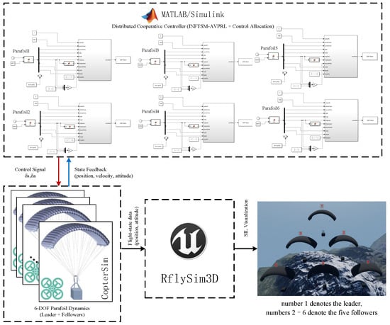
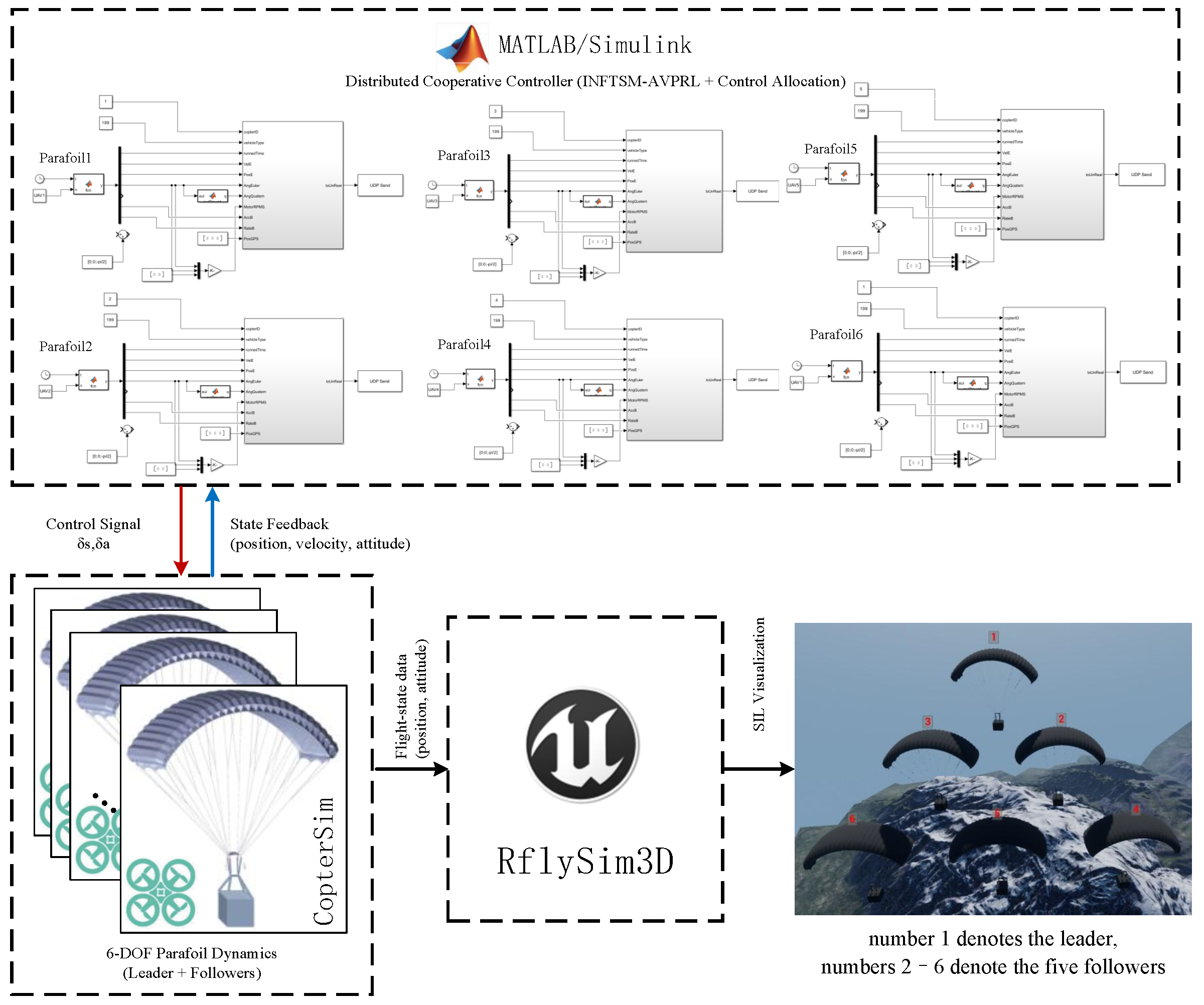
To evaluate the proposed INFTSM cooperative-control strategy under modeled physical constraints and random gust disturbances, a software-in-the-loop (SIL) co-simulation platform is constructed using MATLAB/Simulink R2023b and the RflySim simulation environment [29,30] (Figure 4). The simulation object is set as a 6-DOF parafoil swarm consisting of one leader parafoil and five follower parafoils.

Figure 4. RflySim software-in-the-loop swarm simulation.

To further clarify the control structure of the software-in-the-loop simulation, the multi-parafoil closed-loop system is implemented in MATLAB/Simulink using four sequential layers: a guidance layer, a graph-based cooperative-control layer, a control-allocation and actuator layer, and a 6-DOF dynamics layer. CopterSim is used to exchange steering-line commands and simulated vehicle-state data bidirectionally within the closed SIL loop, while RflySim provides three-dimensional visualization. For the leader parafoil, the guidance layer employs the Stanley-type trajectory-tracking method described in Section 3.1. The lateral cross-track error and longitudinal altitude error relative to the reference trajectory are used to generate the commanded speed, heading angle, and flight-path angle. The actual position and velocity produced by the leader’s 6-DOF dynamic model are then supplied to the follower parafoils as reference states, and the corresponding leader acceleration ${\mathit{U}}_0$ is supplied to the cooperative-control layer as the feedforward term in Equation (36). For each follower, the distributed position and velocity errors, ${\mathit{E}}_{p,i}$ and ${\mathit{E}}_{v,i}$, are calculated from its own state and the states available from its neighbors and the leader. The fixed-topology cooperative-control layer assembles these errors and evaluates Equation (36); the resulting block ${\mathit{U}}_{F,i}^{\mathrm{raw}}$ is the raw cooperative acceleration command for follower i. After projection onto the admissible acceleration set, the resulting virtual command ${\mathit{U}}_{\mathrm{eq},i}$ is integrated into a feasible velocity reference and is then mapped by the parafoil control-allocation module into symmetric and asymmetric steering-line commands.

Although each parafoil is represented by a 6-DOF dynamic model, only two independent control channels are physically available: the symmetric and asymmetric steering-line inputs. Therefore, the simulation does not employ the independent PID attitude inner loops commonly used for fixed-wing aircraft. Instead, the roll, pitch, and yaw dynamics are retained in the 6-DOF controlled plant, while the longitudinal and lateral control-allocation paths map the virtual cooperative-control demand into the two physically realizable steering-line commands. Consequently, the attitude states are not independently tracked by a separate attitude controller; they evolve within the closed-loop 6-DOF dynamics under the aerodynamic forces and moments generated by the steering-line inputs. This configuration preserves the strongly coupled flight characteristics of the parafoil and avoids introducing virtual attitude-control channels that are not physically available.

Actuator saturation is implemented in Simulink by clipping the unconstrained normalized line demands ${\overline{\sigma }}_{L,i}$ and ${\overline{\sigma }}_{R,i}$ to $[0,1]$, as specified in Equation (46). The unconstrained demands define ${\delta }_{s,i}^{\mathrm{cmd}}$ and ${\delta }_{a,i}^{\mathrm{cmd}}$, whereas the clipped demands define the actual deflections through Equation (47). Hence, the coupled feasible-region condition in Equation (48) is enforced before the aerodynamic-force and aerodynamic-moment calculations of the 6-DOF plant. The resulting clipping mismatch contributes to the complete command-realization residual defined in Section 4.2, together with projection, command limiting, gusts, and modeling errors.

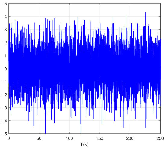
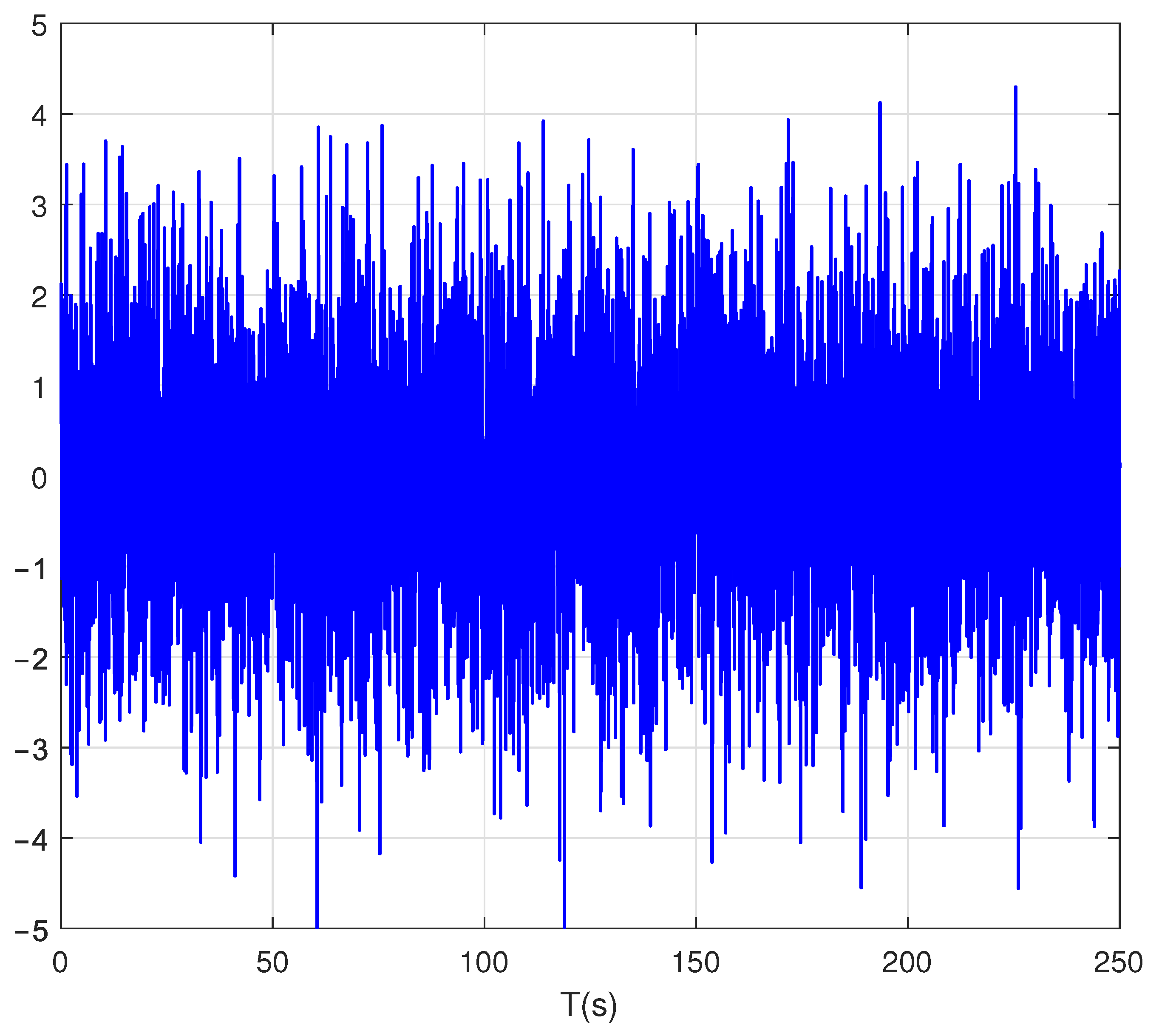
To excite the three-dimensional coupling and dynamic nonlinearity of the system, dispersed initial positions and heading angles are assigned to the follower parafoils (Table 1). Simultaneously, a random gust model containing continuous random fluctuations and high-frequency pulsating components is introduced into the simulation (Figure 5). Together with the modeled aerodynamic mapping and actuator limits, this setup is used to evaluate convergence and tracking performance under the considered nonideal conditions.

Table 1. Initial states of the parafoil swarm.

No.	Initial States
	Coordinates (m)	Heading Angle	Flight-Path Angle
1	$(1500,600,2000)$	${45}^{\circ }$	$-{10}^{\circ }$
2	$(2100,800,2000)$	${65}^{\circ }$
3	$(600,1500,2000)$	${80}^{\circ }$
4	$(1800,900,2000)$	${75}^{\circ }$
5	$(500,1900,2000)$	${105}^{\circ }$
6	$(800,1300,2000)$	${95}^{\circ }$

Note: Parafoil No. 1 is the leader; Nos. 2–6 are followers.

Figure 5. Random gust disturbance.

5.2. Trajectory Evolution and Spatial Convergence Analysis

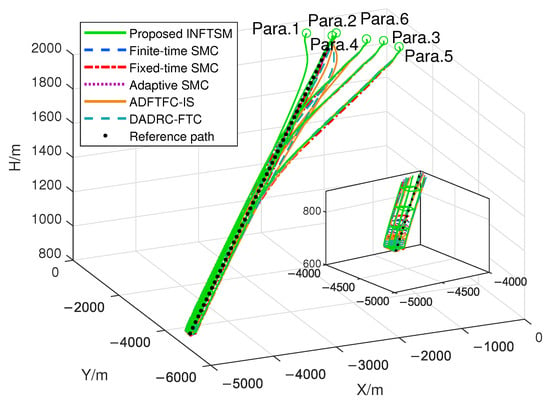
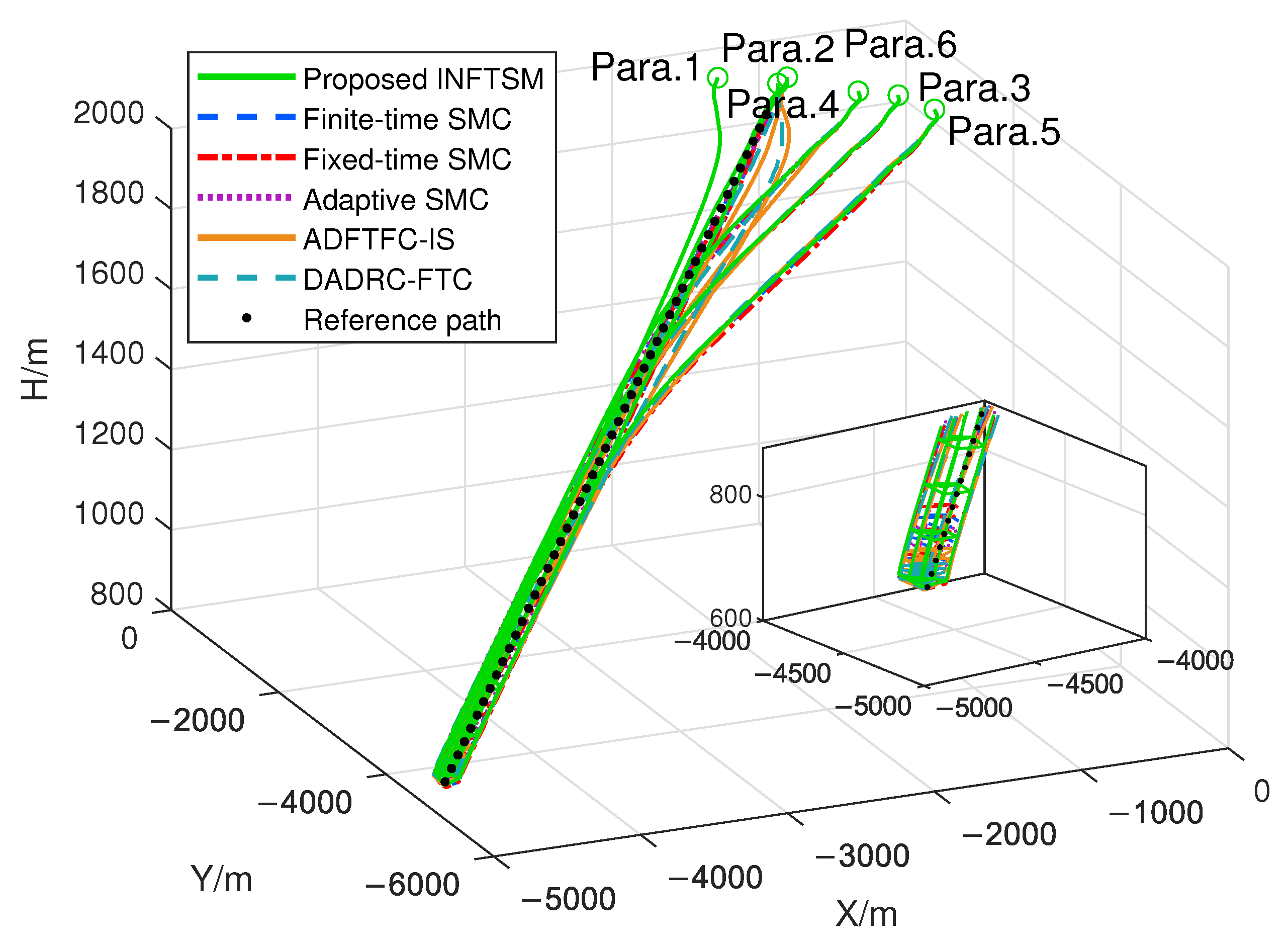
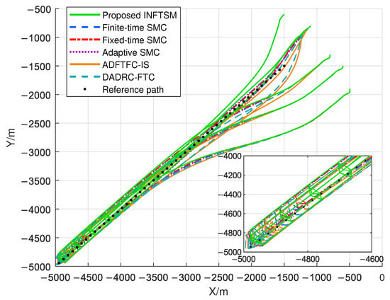
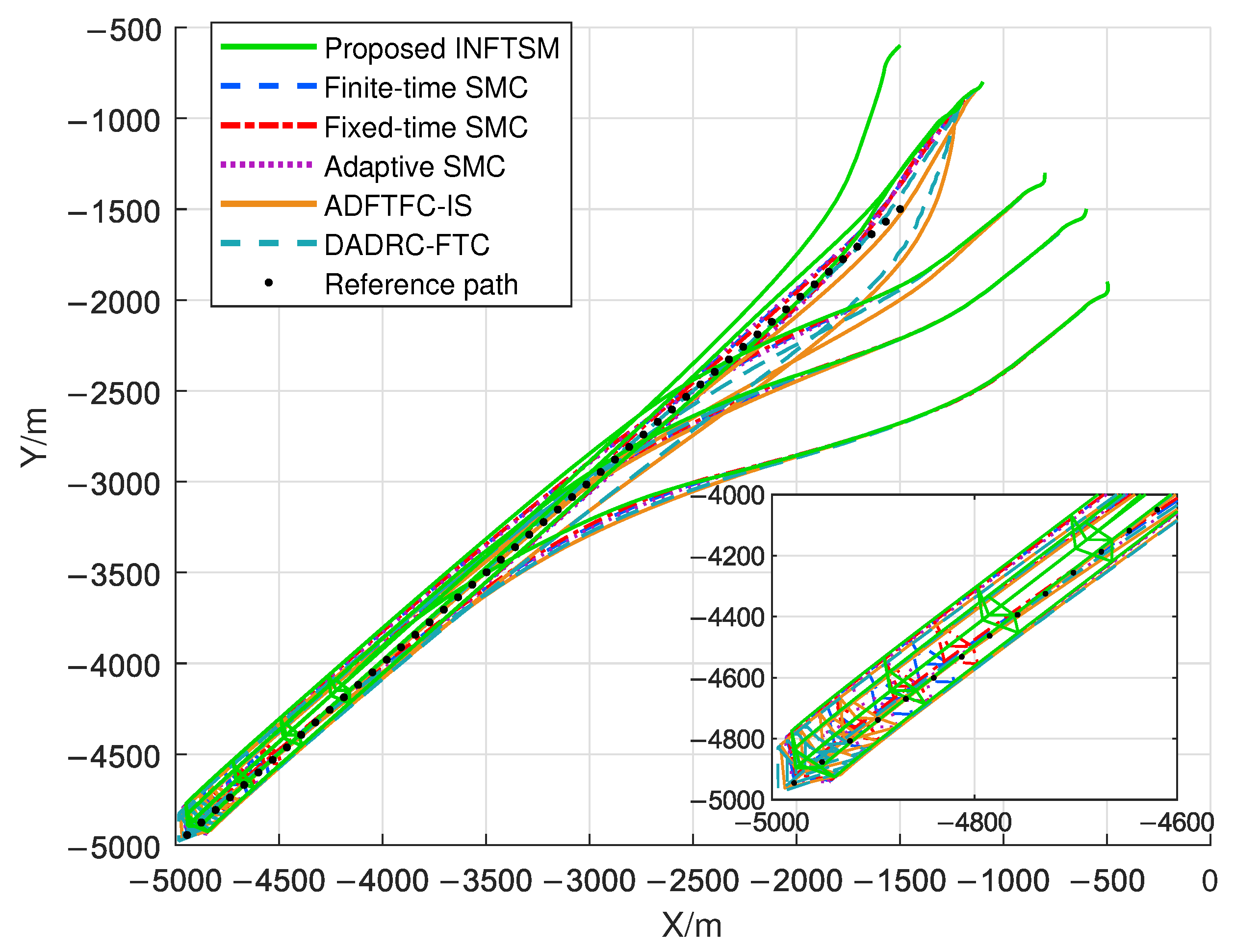
Figure 6 and Figure 7 respectively present the three-dimensional flight trajectories and two-dimensional horizontal projections of the multi-parafoil swarm under six control strategies. The green solid line denotes the proposed INFTSM control strategy; the blue dashed, red dash-dotted, purple dotted, orange solid, and cyan dashed lines denote finite-time SMC, fixed-time SMC, adaptive SMC, ADFTFC-IS, and DADRC-FTC, respectively; and the black dotted line denotes the reference path of the leader parafoil. The triangular connections depict the instantaneous formation configuration of the swarm during flight. To reflect the establishment time according to the adopted plotting criterion, the corresponding geometric connections are plotted only after the mean formation error enters the 50 m error band and remains within it for 5 s. Under dispersed initial positions and gust disturbances, all six compared controllers achieve basic formation tracking within the common 6-DOF parafoil simulation framework.

Figure 6. Three-dimensional flight trajectories of the multi-parafoil swarm under six control strategies.

Figure 7. Two-dimensional horizontal projections of the multi-parafoil swarm trajectories under six control strategies.

However, differences in trajectory evolution remain among the six control strategies. Compared with the other five benchmark methods, the proposed INFTSM produces a relatively compact trajectory-evolution pattern under the considered simulation conditions. Further examination of the spatial distribution of the formation connections shows that the green triangular connections corresponding to INFTSM appear at higher flight altitudes and earlier positions along the flight path. Because the formation connections are plotted only after the mean formation error enters the 50 m error band and remains within it for 5 s, their earlier appearance indicates that INFTSM satisfies the prescribed formation-error criterion sooner.

By contrast, the formation connections corresponding to the other controllers appear later and are accompanied by varying degrees of transient trajectory dispersion. These observations suggest relatively favorable INFTSM behavior in formation establishment and trajectory evolution under the considered 6-DOF model, initial conditions, and gust disturbance. The performance differences among the control strategies are further analyzed below using quantitative metrics.

5.3. Error Quantitative Assessment and Comprehensive Performance Comparison

For quantitative assessment, define the scalar formation-position error of follower i and the mean error over the N followers as

$$e_{\mathrm{form},i}\left(t\right)={\parallel {\tilde{\mathit{P}}}_i\left(t\right)\parallel }_2,{\overline{e}}_{\mathrm{form}}\left(t\right)={\displaystyle \frac{1}{N}}{\displaystyle \sum _{i=1}^N}{e}_{\mathrm{form},i}\left(t\right),$$

(77)

where $N=5$ in the simulations. Let $t_f$ be the final simulation time and $T_w=100\mathrm{s}$ the terminal evaluation window. The performance indicators are defined as

$$T_{\mathrm{set}}^{\left(5\right)}=\inf \left\{t\in [0,t_f-5\mathrm{s}]:{\overline{e}}_{\mathrm{form}}\left(\tau \right)\le 50\mathrm{m}\mathrm{for}\mathrm{all}\tau \in [t,t+5\mathrm{s}]\right\},$$

(78)

$${\mathrm{RMSE}}_{100}={\left({\displaystyle \frac{1}{T_w}}{\int }_{t_f-T_w}^{t_f}{\overline{e}}_{\mathrm{form}}^2\left(t\right)\mathrm{d}t\right)}^{1/2},$$

(79)

$$\mathrm{IAE}={\int }_0^{t_f}{\overline{e}}_{\mathrm{form}}\left(t\right)\mathrm{d}t.$$

(80)

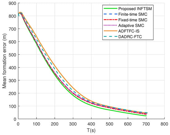
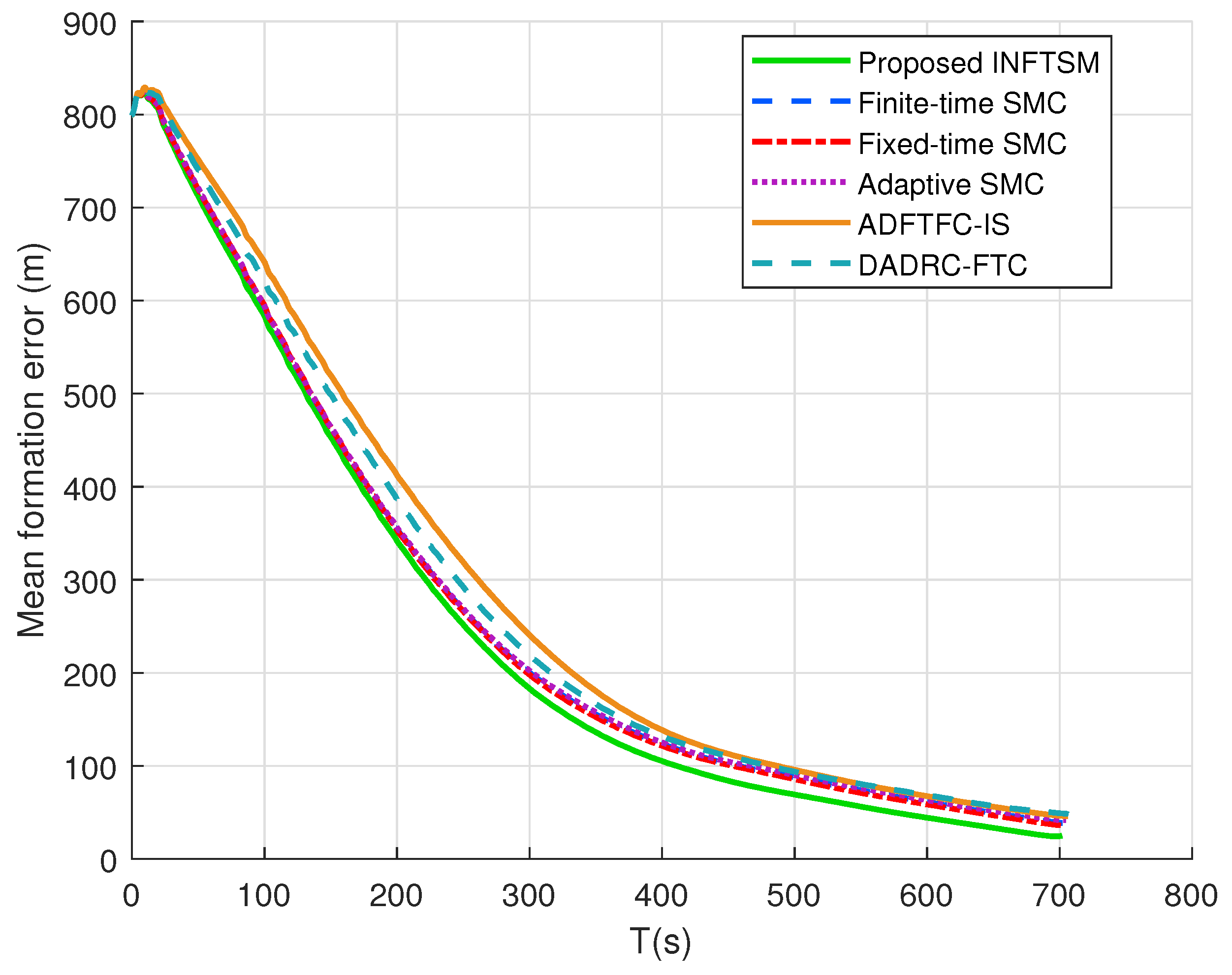
The settling time is assigned $+\infty$ if the set in Equation (78) is empty. Figure 8 shows ${\overline{e}}_{\mathrm{form}}\left(t\right)$, and Figure 9 compares the three indicators for all six controllers.

Figure 8. Mean formation error.

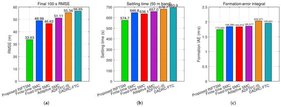
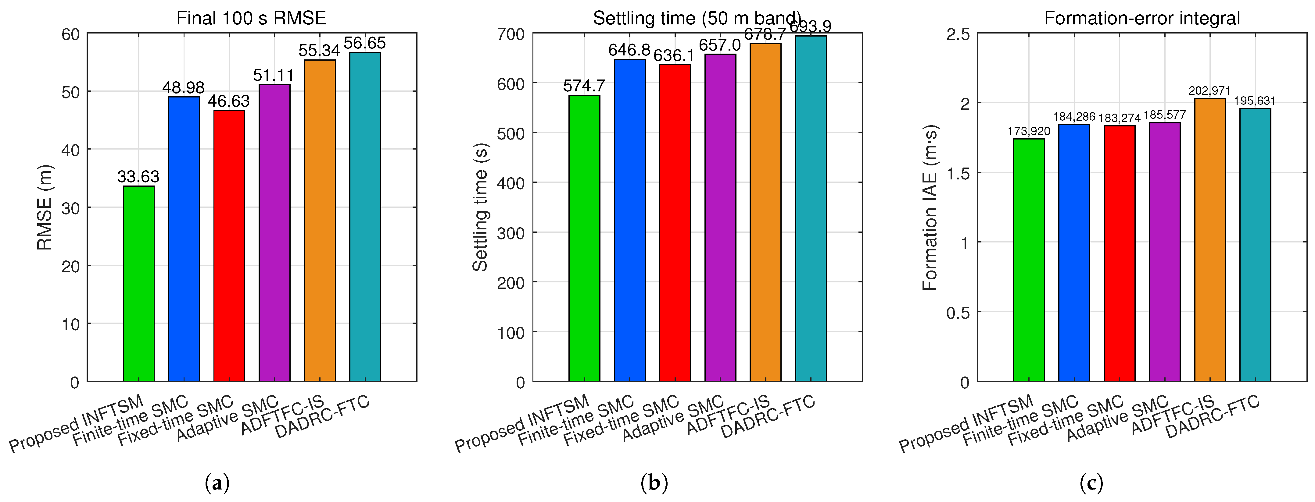
Figure 9. Comparison of comprehensive performance indicators of the parafoil formation system for the six controllers: (a) RMSE over the final 100 s; (b) settling time for the 50 m error band; and (c) integral of absolute formation error.

Among the six controllers compared in Figure 9, the proposed INFTSM achieves lower values for all three evaluation metrics under the considered deterministic simulation conditions. Its ${\mathrm{RMSE}}_{100}$ is 33.63 m, corresponding to reductions of 31.34%, 27.88%, 34.20%, 39.23%, and 40.64% relative to finite-time SMC, fixed-time SMC, adaptive SMC, ADFTFC-IS, and DADRC-FTC, respectively. Its settling time is 574.7 s, representing reductions of 11.15%, 9.65%, 12.53%, 15.32%, and 17.18% against the same five benchmark controllers. In addition, its IAE is 173,920 m·s, which is 5.62%, 5.10%, 6.28%, 14.31%, and 11.10% lower, respectively. Taken together, these results indicate that the proposed INFTSM provides favorable performance in tracking accuracy, convergence speed, and accumulated formation error for the considered simulation scenario. The same six-controller comparison is further examined statistically through the subsequent 200-trial Monte Carlo study.

5.4. 6-DOF Physical Response and Control-Activity Assessment

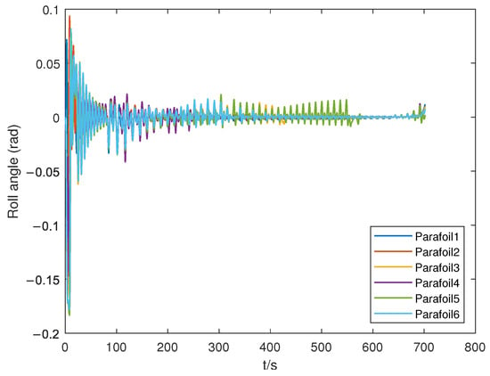
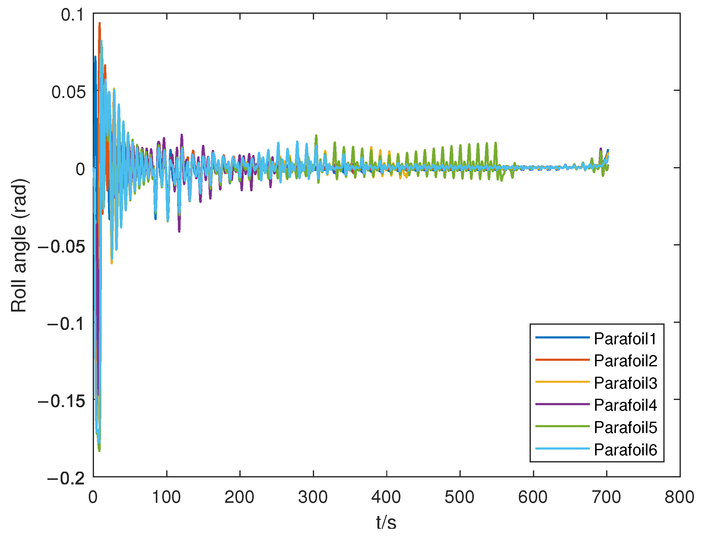
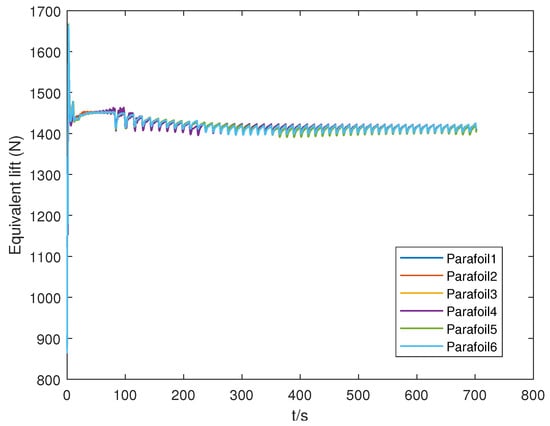
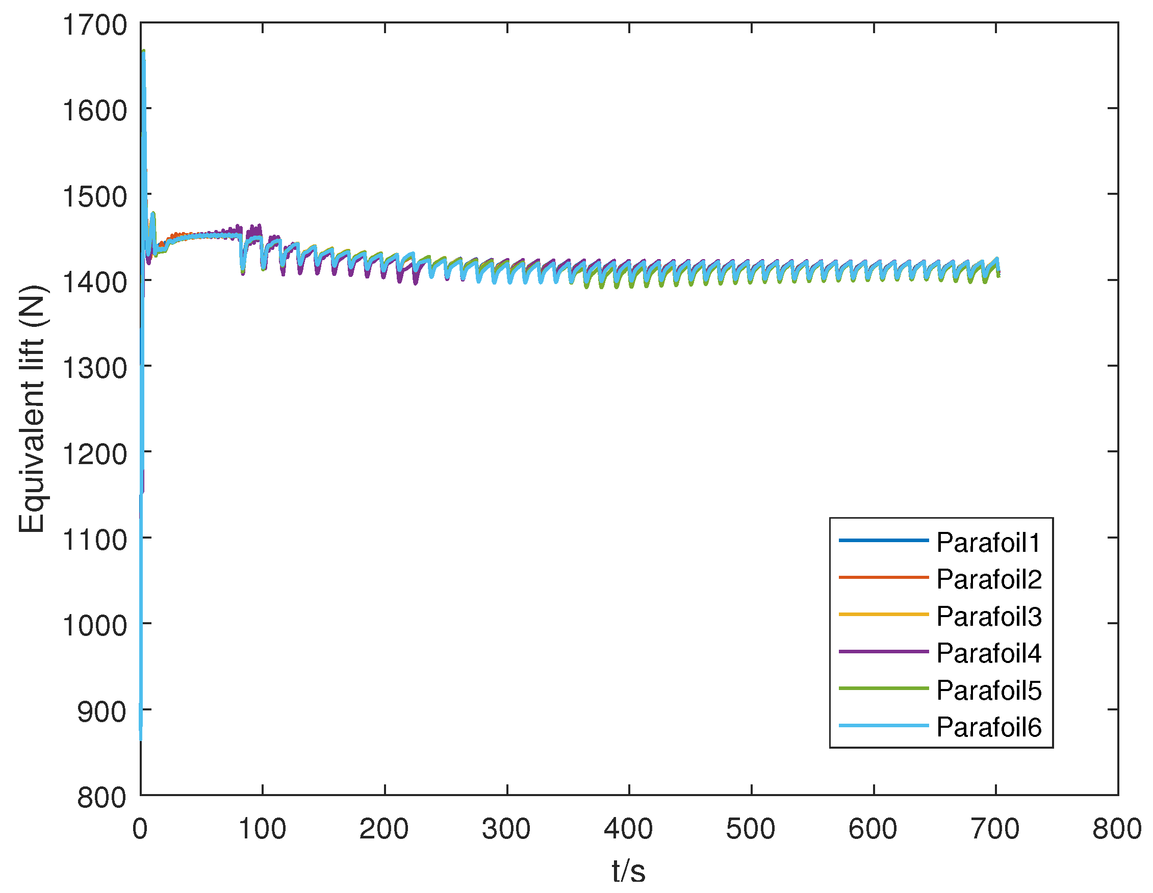
Formation-tracking performance should be interpreted together with the underlying physical responses. Therefore, Figure 10, Figure 11 and Figure 12 present the 6-DOF responses of the six parafoils under INFTSM control, including the three-axis acceleration, roll angle ${\phi }_i$, and equivalent lift.

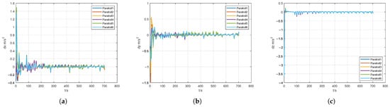
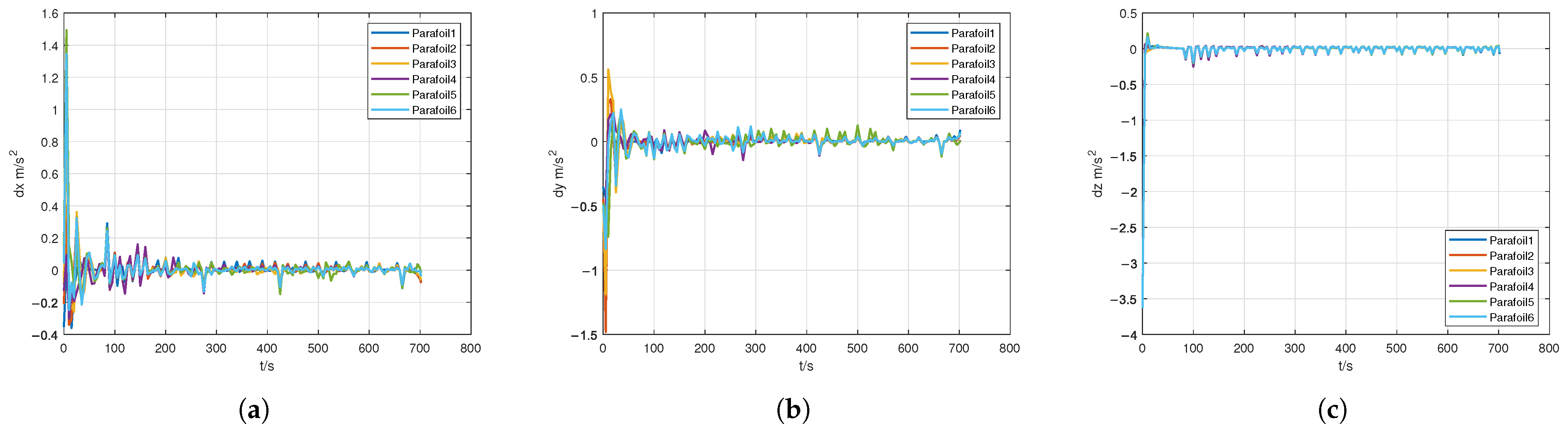
Figure 10. Parafoil accelerations along the three axes: (a) x-axis acceleration; (b) y-axis acceleration; and (c) z-axis acceleration.

Figure 11. Actual roll angle ${\phi }_i$.

Figure 12. Equivalent lift.

The comparatively pronounced roll oscillations in Figure 11 occur mainly during the initial formation-acquisition stage. Because the parafoils start from dispersed positions with different initial heading angles, relatively large and alternating heading corrections are required to reduce the initial formation errors. These corrections generate transient differential steering-line inputs and excite the coupled roll–yaw dynamics of the parafoil system. To mitigate this response, the feasible-command inner loop imposes envelope and rate limits on the commanded speed, flight-path angle, and heading angle through Equations (40) and (41), bounds the integral states through Equation (44), and incorporates roll-rate feedback into the heading-control contribution in Equation (45) to enhance lateral damping. Under identical initial conditions and disturbance settings, these modifications reduce the maximum absolute roll angle from 0.183 to 0.162 rad. The latest time after which all parafoils enter and remain within the $\pm 0.02$ rad band is reduced from 146.6 to 117.1 s. These results indicate that the revised inner-loop implementation effectively reduces transient roll oscillations during formation acquisition under the considered simulation conditions.

Figure 10 shows that the initial formation-reconfiguration stage (0–100 s) produces transient peaks in the three-axis accelerations. As the formation error decreases, the acceleration amplitudes gradually attenuate, with the 50 m error-band and 5 s dwell criterion satisfied at 574.7 s. As discussed for Figure 11, the revised roll response remains bounded after the initial transient. Figure 12 further shows that the equivalent lift remains between 1.41 kN and 1.45 kN after the initial transient. Collectively, these results show bounded 6-DOF physical responses under the considered gust disturbances and steering-line constraints. The corresponding actuator activity is quantified next.

Table 2 quantifies the actual post-clipping normalized left- and right-steering-line commands using their maximum, root-mean-square (RMS), saturation percentage, and maximum continuous saturation duration. The maximum and RMS combine both channels; the saturation percentage is the fraction of follower–channel–time samples at either normalized command limit, 0 or 1; and the duration is the longest uninterrupted interval for which either channel remains at a limit.

Table 2. Statistics of the actual normalized steering-line commands for the five follower parafoils under INFTSM.

Follower Parafoil	Maximum Command (–)	RMS Command (–)	Saturation (%)	Maximum Saturation Duration (s)
Parafoil 2	1.000	0.772	0.091	1.20
Parafoil 3	1.000	0.799	0.587	6.64
Parafoil 4	1.000	0.869	0.799	10.06
Parafoil 5	1.000	0.869	0.578	4.28
Parafoil 6	1.000	0.855	0.653	6.05
All followers	1.000	0.834	0.542	10.06

Note: Steering-line commands are normalized to $[0,1]$. A command is considered to be at a saturation boundary when its value is within ${10}^{-6}$ of either limit. For each follower, the maximum and RMS values are calculated from the combined left- and right-command samples. The overall saturation percentage is calculated as $P_{\mathrm{sat}}=N_{\mathrm{bound}}/\left(10N\right)\times 100\%$, where $N_{\mathrm{bound}}$ is the total number of boundary samples across all ten steering-line channels and N is the number of samples per channel. The maximum continuous saturation duration is calculated as $T_{\max }=N_{\max }\times \Delta t$, where $N_{\max }$ is the longest consecutive boundary-sample count on any single channel and $\Delta t$ is the sampling interval.

As shown in Table 2, the aggregate maximum and RMS commands of the five followers are 1.000 and 0.834, respectively. The aggregate saturation percentage is 0.542%, and the longest continuous saturation event lasts 10.06 s. All five followers reach a steering-line command limit. These results show that the actuator constraints are encountered in the simulated command histories rather than acting as inactive saturation blocks. Together with the formation-error results, the statistics quantify the controller behavior under actively enforced steering-line limitations in the considered deterministic simulation.

5.5. Monte Carlo Statistical Performance Analysis

To evaluate statistical performance beyond a single initial state or gust realization, 200 paired Monte Carlo trials were conducted with randomized initial conditions and stochastic gust disturbances. In each trial, a new randomized initial condition and an independent three-dimensional colored-gust realization were generated. Within the same trial, all controllers were evaluated using the same randomized initial states and gust sequence, providing a consistent paired comparison.

The nominal initial states are those listed in Table 1. For every parafoil, independent uniform perturbations were applied to the nominal values: the horizontal-position components were perturbed within $\pm 50$ m, altitude within $\pm 20$ m, initial airspeed within $\pm 0.30$ m/s, heading angle within $\pm 5^{\circ }$, and flight-path angle within $\pm 2^{\circ }$. A temporally correlated three-dimensional colored-gust sequence was regenerated with an independent random seed for every Monte Carlo trial. Six controllers were compared: the proposed INFTSM, finite-time SMC, fixed-time SMC, adaptive SMC, ADFTFC-IS, and DADRC-FTC. All methods used the same 6-DOF parafoil dynamics, Stanley-type leader-guidance law, reference trajectory, communication topology, control-allocation and actuator configuration, steering-line constraints, controller update period, and simulation step size. Only the outer-loop formation-control law differed among the six methods. All controller parameters were fixed before the Monte Carlo campaign and were not retuned for individual trials.

For each trial, the final 100 s RMSE, IAE, conditional settling time, maximum outer-loop formation-control effort $E_{\max }$, and actuator saturation percentage were recorded. Here, $E_{\max }$ is the maximum magnitude of the outer-loop formation-induced velocity correction, excluding the common leader/path feedforward component; it is therefore not a physical steering-line input. Conditional settling time was calculated for trials in which the formation RMSE remained within 20 m for at least 10 consecutive seconds. The saturation percentage was calculated as the fraction of sampled follower–channel–time points at which the corresponding unconstrained line demand lay outside $[0,1]$ and clipping was activated. Except for conditional settling time, the statistics in Table 3 are reported as the sample mean ± standard deviation over all 200 paired trials.

Table 3. Monte Carlo statistics of the six controllers over 200 paired trials (mean ± standard deviation).

Controller	Final 100 s RMSE (m)	IAE ($\mathbf{m}·\mathbf{s}$)	Conditional Settling Time (s)	Maximum Outer-Loop Formation-Control Effort, ${\mathit{E}}_{\max }$ (m/s)	Saturation (%)
Proposed INFTSM	$58.706$$\pm 31.984$	$210,732.9$$\pm 19,057.6$	$629.29$$\pm 38.16$	$9.414$$\pm 0.226$	$1.046$$\pm 0.191$
Finite-time SMC	$71.562$$\pm 33.170$	$221,156.6$$\pm 19,040.6$	$639.24$$\pm 25.79$	$9.383$$\pm 0.225$	$1.062$$\pm 0.182$
Fixed-time SMC	$67.449$$\pm 31.334$	$219,961.9$$\pm 18,427.3$	$642.72$$\pm 25.35$	$9.336$$\pm 0.223$	$1.095$$\pm 0.211$
Adaptive SMC	$76.024$$\pm 34.370$	$222,892.0$$\pm 19,486.2$	$644.02$$\pm 28.44$	$9.378$$\pm 0.225$	$1.086$$\pm 0.215$
ADFTFC-IS	$87.115$$\pm 32.592$	$245,093.7$$\pm 18,265.0$	$654.34$$\pm 18.72$	$9.491$$\pm 0.231$	$0.757$$\pm 0.215$
DADRC-FTC	$89.052$$\pm 32.509$	$235,301.0$$\pm 19,661.7$	$664.33$$\pm 19.72$	$9.535$$\pm 0.232$	$3.891$$\pm 0.881$

Note: Results are reported as mean ± standard deviation. $E_{\max }$ denotes the maximum magnitude of the outer-loop formation-induced velocity correction, excluding the common leader/path feedforward component, rather than the physical steering-line input. Conditional settling time is calculated only for trials in which the formation RMSE remains within 20 m for at least 10 consecutive seconds. The numbers of trials satisfying this criterion are 46, 23, 23, 22, 5, and 7 out of 200 for the six controllers, respectively, in the order listed in the table. All other metrics are evaluated over the complete 200 trials.

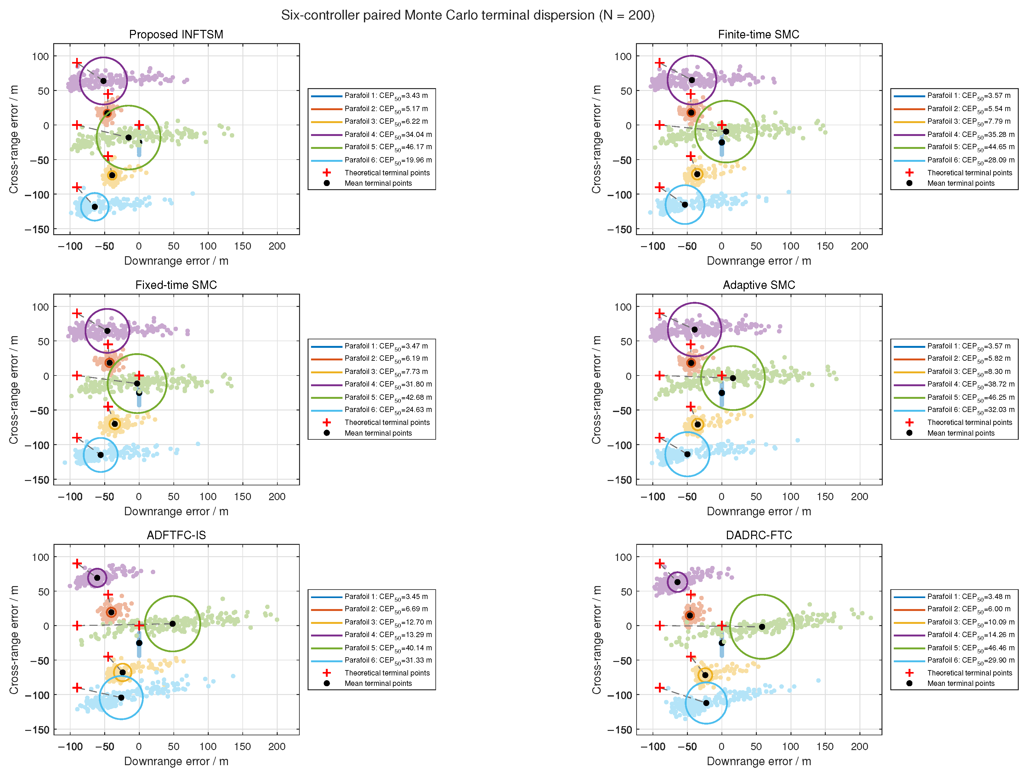
Figure 13 shows bounded terminal-position dispersion for all six controllers under the randomized initial states and gust realizations considered. In comparison, the proposed INFTSM produces more concentrated terminal-position distributions for most formation members. The 50% circular error probable (${\mathrm{CEP}}_{50}$) values of Parafoils 1, 2, 3, and 6 are approximately 3.43 m, 5.17 m, 6.22 m, and 19.96 m, respectively. The terminal dispersion is not identical for all members because each parafoil is affected differently by its spatial position, neighborhood connections, and terminal formation-reconstruction process. Therefore, ${\mathrm{CEP}}_{50}$ is used primarily to characterize the statistical terminal dispersion of individual members, whereas the overall controller performance is evaluated using RMSE, IAE, conditional settling time, and actuator-related metrics.

Figure 13. Terminal-position dispersion over 200 paired Monte Carlo trials for the six controllers. Colored circles denote the corresponding ${\mathrm{CEP}}_{50}$ boundaries centered at the mean terminal points; red plus signs and black dots indicate the theoretical and mean terminal points, respectively.

As shown in Table 3, the proposed INFTSM has the lowest final 100 s RMSE, IAE, and mean conditional settling time among the six compared controllers. Its final 100 s RMSE is $58.706\pm 31.984$ m. Relative to finite-time SMC, fixed-time SMC, and adaptive SMC, the mean RMSE is reduced by approximately 17.96%, 12.96%, and 22.78%, respectively. Relative to ADFTFC-IS and DADRC-FTC, the reductions are approximately 32.61% and 34.08%, indicating lower steady-state formation error under the randomized conditions considered.

The proposed method also yields the lowest IAE, 210,732.9 ± 19,057.6 $\mathrm{m}·\mathrm{s}$, among the six controllers. Compared with ADFTFC-IS and DADRC-FTC, its mean IAE is reduced by approximately 14.02% and 10.44%, respectively. This result indicates a smaller accumulated formation error over the simulated formation-assembly and trajectory-tracking interval.

In terms of dynamic convergence, the mean conditional settling time of INFTSM is $629.29\pm 38.16$ s, shorter than those of the other five methods. Compared with ADFTFC-IS and DADRC-FTC, the mean conditional settling time is reduced by approximately 3.83% and 5.27%, respectively. Together with the deterministic simulation, these results are consistent with the intended controller behavior: larger sliding-variable magnitudes invoke a larger reaching gain, whereas the gain approaches its prescribed minimum near the sliding manifold.

The maximum outer-loop formation-control efforts of the six controllers remain within approximately 9.3–9.5 m/s, and the proposed INFTSM yields $E_{\max }=9.414\pm 0.226$ m/s, comparable to those of the benchmark controllers. Its actuator saturation percentage is $1.046\pm 0.191$%, lower than the $3.891\pm 0.881$% obtained with DADRC-FTC. Although ADFTFC-IS has the lowest saturation percentage, $0.757\pm 0.215$%, its RMSE, IAE, and conditional settling time are higher than those of INFTSM in these trials. Thus, the proposed controller provides lower formation error and shorter conditional settling time without a marked increase in outer-loop formation-control effort or actuator saturation percentage under the tested conditions.

Overall, the 200-trial Monte Carlo statistics are consistent with the representative deterministic simulation. Under the randomized initial conditions and colored-gust realizations considered, the proposed INFTSM provides favorable formation accuracy, accumulated-error performance, and convergence speed. Although individual benchmark methods perform better for a particular actuator metric, INFTSM gives a balanced numerical tradeoff among RMSE, IAE, conditional settling time, maximum outer-loop formation-control effort, and saturation percentage within the tested simulation range.

6. Conclusions

This study developed an INFTSM–AVPRL formation-control framework for multi-parafoil systems subject to wind disturbances and steering-line saturation. Under the stated assumptions, the Lyapunov- and homogeneity-based analyses establish nominal finite-time convergence within the prescribed operating region and a local practical finite-time bound for bounded residual disturbances. The current fixed-topology SIL realization evaluates the ${\mathit{H}}^{-1}$ operation at the network cooperative-control layer; a fully decentralized realization remains to be investigated.

The proposed method was further evaluated in a six-parafoil MATLAB/Simulink–RflySim software-in-the-loop environment through deterministic comparative simulations and 200 paired Monte Carlo trials. In the Monte Carlo comparison under the considered initial-condition variations, gust disturbances, and steering-line constraints, the proposed controller yielded lower formation-error RMSE and shorter conditional settling time than the selected benchmark methods while maintaining a low actuator saturation percentage. These SIL results indicate the feasibility and comparative numerical performance of the proposed approach within the simulated parameter ranges and disturbance environment; they do not constitute physical or experimental validation.

Several limitations remain. First, the proposed method has not yet been validated through hardware-in-the-loop tests or outdoor flight experiments. Second, the theoretical analysis assumes a fixed, delay-free, and packet-loss-free communication network and does not address asynchronous sampling or switching topologies. Third, collision avoidance and inter-agent safety constraints are not explicitly incorporated into the current formation-control framework. Sensor noise, state-estimation errors, and actuator dynamics beyond the modeled steering-line saturation are also not considered explicitly. Finally, the 6-DOF parafoil model is formulated under a rigid-composite canopy–payload assumption and does not include canopy deformation or relative canopy–payload pendular motion as independent degrees of freedom. Future work will therefore investigate experimental validation, communication-impaired formation control, collision avoidance, noise-aware state estimation, and models that explicitly incorporate canopy flexibility and relative canopy–payload dynamics.

References

- Sun, Q.; Yang, J.; Sun, H.; Chen, Z. Review of key technologies for autonomous homing of parafoil systems. J. Natl. Univ. Def. Technol. 2024, 46, 1–15. (In Chinese) [Google Scholar] [CrossRef]
- Chen, Q.; Zhao, M.; Zhao, Z.H.; Ma, M.; Huang, R. Multiple autonomous parafoils system modeling and rendezvous control. Acta Aeronaut. Astronaut. Sin. 2016, 37, 3121–3130. (In Chinese) [Google Scholar] [CrossRef]
- Zuo, Z.; Han, Q.L.; Ning, B.; Ge, X.; Zhang, X.-M. An overview of recent advances in fixed-time cooperative control of multiagent systems. IEEE Trans. Ind. Inform. 2018, 14, 2322–2334. [Google Scholar] [CrossRef] [Scilit]
- Zhu, H.; Sun, Q.; Liu, X.; Liu, J.; Sun, H.; Wu, W.; Tan, P.; Chen, Z. Fluid–structure interaction-based aerodynamic modeling for flight dynamics simulation of parafoil system. Nonlinear Dyn. 2021, 104, 3445–3466. [Google Scholar] [CrossRef] [Scilit]
- Yan, L.; Song, Y.; Wang, H.; Shi, Z.; Song, Y. Dynamic trajectory planning for autonomous parafoil homing under wind disturbances. Aerospace 2026, 13, 276. [Google Scholar] [CrossRef] [Scilit]
- Bae, Y.B.; Lim, Y.H.; Ahn, H.S. Distributed robust adaptive gradient controller in distance-based formation control with exogenous disturbance. IEEE Trans. Autom. Control 2021, 66, 2868–2874. [Google Scholar] [CrossRef] [Scilit]
- Yang, J.S.; Lu, W.T.; Sun, Q.L.; Sun, H.; Chen, Z. Sliding mode control of parafoil systems based on extended state observer. Spacecr. Recovery Remote Sens. 2025, 46, 14–24. (In Chinese) [Google Scholar] [CrossRef]
- Silva, A.L.; Santos, D.A. Fast nonsingular terminal sliding mode flight control for multirotor aerial vehicles. IEEE Trans. Aerosp. Electron. Syst. 2020, 56, 4288–4299, Erratum in IEEE Trans. Aerosp. Electron. Syst. 2021, 57, 3549–3549. https://doi.org/10.1109/TAES.2021.3111717. [Google Scholar] [CrossRef] [Scilit]
- Zhang, J.; Zhang, P.; Yan, J. Distributed adaptive finite-time compensation control for UAV swarm with uncertain disturbances. IEEE Trans. Circuits Syst. I Regul. Pap. 2021, 68, 829–841. [Google Scholar] [CrossRef] [Scilit]
- Sun, Q.; Yu, L.; Zheng, Y.; Tao, J.; Sun, H.; Sun, M.; Dehmer, M.; Chen, Z. Trajectory tracking control of powered parafoil system based on sliding mode control in a complex environment. Aerosp. Sci. Technol. 2022, 122, 107406. [Google Scholar] [CrossRef] [Scilit]
- Sun, R.; Zhou, Z.; Zhu, X. Flight quality characteristics and observer-based anti-windup finite-time terminal sliding mode attitude control of aileron-free full-wing configuration UAV. Aerosp. Sci. Technol. 2021, 112, 106638. [Google Scholar] [CrossRef] [Scilit]
- Liu, B.; Li, A.; Guo, Y.; Wang, C. Adaptive distributed finite-time formation control for multi-UAVs under input saturation without collisions. Aerosp. Sci. Technol. 2022, 120, 107252. [Google Scholar] [CrossRef] [Scilit]
- Chen, T.; Lei, Y.; Peng, H.; Chen, Y.; Chai, X.; Zhang, Z. Finite-time anti-saturated formation tracking control of multiple unmanned aerial vehicles: A performance tuning way. Mathematics 2023, 11, 4255. [Google Scholar] [CrossRef] [Scilit]
- Wang, P.; Zhang, X.; Ge, S.S. Prescribed-time control with explicit reference governor for a class of constrained cascaded systems. Int. J. Robust. Nonlinear Control 2021, 31, 6422–6437. [Google Scholar] [CrossRef] [Scilit]
- Tartaglione, G.; Nicotra, M.M.; Naldi, R.; Garone, E. A constrained control framework for unmanned aerial vehicles based on explicit reference governor. Automatica 2024, 166, 111696. [Google Scholar] [CrossRef] [Scilit]
- Chen, Q.J.; Jin, Y.Q.; Yan, T.L.; Wang, T.Y.; Wang, Y. UAV formation control under communication constraints based on distributed model predictive control. Math. Probl. Eng. 2022, 2022, 7316009. [Google Scholar] [CrossRef] [Scilit]
- Wei, S.Z.; Sun, H.; Sun, Q.L. Homing trajectory prediction of parafoil based on dynamic intelligent simulation. Spacecr. Recovery Remote Sens. 2025, 46, 25–34. (In Chinese) [Google Scholar] [CrossRef]
- Zhao, L.G.; He, W.L.; Du, Y.J. Dynamic parameter identification of parafoil systems based on sensitivity analysis. Spacecr. Recovery Remote Sens. 2022, 43, 26–39. (In Chinese) [Google Scholar] [CrossRef]
- Zhao, L.; He, W.; Lv, F. Model-free adaptive control for parafoil systems based on the iterative feedback tuning method. IEEE Access 2021, 9, 35900–35914. [Google Scholar] [CrossRef] [Scilit]
- Feng, Q.; Zhang, Q.; Feng, Z.; Ge, J.; Chen, Q.; Li, L.; Huang, Y. Stochastic model predictive control for parafoil system via Markov-based multi-scenario optimization. Aerospace 2025, 12, 810. [Google Scholar] [CrossRef] [Scilit]
- Li, Y.; Zhao, M.; Chen, Q.; Yao, M.; He, Z. Combined trajectory planning of parafoil systems in complex environments. Acta Aeronaut. Astronaut. Sin. 2021, 42, 324566. (In Chinese) [Google Scholar] [CrossRef]
- Chen, Q.; Zhao, M.; Li, Y.H.; He, Z.Y. Optimal segment constant trajectory planning for parafoil system based on gradient descent method. Acta Aeronaut. Astronaut. Sin. 2020, 41, 324226. (In Chinese) [Google Scholar] [CrossRef]
- Guo, Y.M.; Yan, J.G.; Xing, X.J.; Wu, C.; Chen, X.; Li, F. Modeling and analysis of deformed parafoil recovery system. J. Northwest. Polytech. Univ. 2020, 38, 952–958. (In Chinese) [Google Scholar] [CrossRef] [Scilit]
- Yao, M.; Cao, Z.; Guo, R.; Zhao, M.; Chen, Y. Nonlinear velocity control strategy and trajectory planning for parafoils using a restricted 6-DOF model. J. Aerosp. Eng. 2025, 38, 04025047. [Google Scholar] [CrossRef] [Scilit]
- Zheng, Y.; Tao, J.; Sun, Q.; Sun, H.; Chen, Z.; Sun, M.; Xie, G. Sideslip angle estimation based active disturbance rejection 3D trajectory tracking control for powered parafoil system and hardware-in-the-loop simulation verification. Aerosp. Sci. Technol. 2023, 141, 108497. [Google Scholar] [CrossRef] [Scilit]
- Bhat, S.P.; Bernstein, D.S. Geometric homogeneity with applications to finite-time stability. Math. Control. Signals Syst. 2005, 17, 101–127. [Google Scholar] [CrossRef] [Scilit]
- Bhat, S.P.; Bernstein, D.S. Continuous finite-time stabilization of the translational and rotational double integrators. IEEE Trans. Autom. Control 1998, 43, 678–682. [Google Scholar] [CrossRef] [Scilit]
- Andrieu, V.; Praly, L.; Astolfi, A. Homogeneous approximation, recursive observer design, and output feedback. SIAM J. Control Optim. 2008, 47, 1814–1850. [Google Scholar] [CrossRef] [Scilit]
- Dai, X.; Ke, C.; Quan, Q.; Cai, K.-Y. RFlySim: Automatic test platform for UAV autopilot systems with FPGA-based hardware-in-the-loop simulations. Aerosp. Sci. Technol. 2021, 114, 106727. [Google Scholar] [CrossRef] [Scilit]
- Dai, X.; Tu, J.; Quan, Q. RflySim ToolChain: A rapid development and validation toolchain for intelligent unmanned swarm systems. J. Syst. Eng. Electron. 2025, 36, 1077–1093. [Google Scholar] [CrossRef] [Scilit]
Disclaimer/Publisher’s Note: The statements, opinions and data contained in all publications are solely those of the individual author(s) and contributor(s) and not of MDPI and/or the editor(s). MDPI and/or the editor(s) disclaim responsibility for any injury to people or property resulting from any ideas, methods, instructions or products referred to in the content. |
© 2026 by the authors. Licensee MDPI, Basel, Switzerland. This article is an open access article distributed under the terms and conditions of the Creative Commons Attribution (CC BY) license.