Corridor-Protected Control Strategy for Tilt-Wing eVTOLs

Abstract

Tilt-wing electric vertical take-off and landing (eVTOL) aircraft face distinctive safety challenges during transition due to configuration variations, highly nonlinear aerodynamics and coupled effects of distributed electric propulsion. These characteristics impose substantial design efforts when conventional envelope protection methods are applied. This paper proposes a transition-corridor-based protected control framework which is compatible with both nonlinear model-based control and conventional feedback control. First, a transition corridor prediction method incorporating electric propulsion constraints is presented, yielding pitch angle and pitch angular acceleration limits as limit commands. Second, a corridor-based protected control strategy is established and integrated into incremental nonlinear dynamic inversion (INDI) and proportional–integral–derivative (PID) controllers. Furthermore, a comparative study is conducted across different protection strategies and controllers to assess the proposed protected control method in safety-critical transition flight. Simulation results demonstrate that the proposed method provides effective protection while exploiting available maneuvering margins. Moreover, incorporating electric propulsion constraints improves the physical consistency of corridor prediction and envelope protection. Overall, this study provides a practical framework for integrating and evaluating corridor-based protection control, facilitating safer transition flight for tilt-wing eVTOL aircraft.

1. Introduction

Manned tilted-thrust eVTOL demonstrators represented by Airbus Vahana [1] and Joby Aviation [2] hold the promise of Advanced Air Mobility (AAM) and have stimulated research interest in tilted-thrust eVTOL configurations. The tilted-thrust mechanism gives rise to complex dynamic transients, pronounced aerodynamic nonlinearities [3] and strong aero-propulsive interactions [4]. These characteristics induce response deviations and diminished safety margins [5,6], posing substantial challenges to control design, which make transition a safety-critical flight phase. Therefore, transition control requires both satisfactory control performance and safety considerations. The development of safe transition control techniques focuses on two aspects: more accurate prediction of admissible region and more effective flight-envelope-protection (FEP) control. For transition feasibility prediction, recent studies have progressed toward better practicality with multi-dimensional constraint integration [7] and dynamic reachability [8,9], which provided a solid basis for control strategy optimization [10,11] and trajectory optimization [7]. Meanwhile, different from conventional fuel-powered aircraft, electric limitations jointly affect the safe boundaries of eVTOL [12]. Recent studies have increasingly incorporated electric constraints. Ogden and Patterson [13] showed that SOC and propulsion response delays reduce system bandwidth and phase margin, thereby degrading flight qualities. Lu [14], Han [15], May [16] et al. further illustrated that motor and actuator dynamics modify the attainable moment set to affect controllable regions. Moreover, instead of nominal-efficiency estimation [17], a component-level electric constraint model should be introduced to capture the coupled drivetrain dynamics [18,19,20].

For FEP focus, flow separation is one of the most critical cases to be avoided for tilt-wing eVTOLs. A nose-up maneuver is required in later transition to build up lift and initial retransition to sustain flow attachment. This results in high risk of unexpected stall [21]. Hence, pitch protection has emerged as one of the most prevalent research themes. Regular protection adopts hard limits that fail to accommodate envelope variations. Lombaerts et al. [22] applied online-estimated envelopes to constrain $C^{*}$, pitch angle and roll angle by imposing command constraints. However, problems including overshoot at bounds and heavy workload of gain scheduling at near-boundary conditions are difficult to avoid [23] because this kind of FEP functions is still a separate layer superimposed to the controller. This motivates the introduction of nonlinear FEP control methods.

For eVTOL applications, INDI provides a promising basis for FEP control due to its reduced model dependence and demonstrated effectiveness in eVTOL flight control [24,25,26]. Stougie et al. [27] extended the NDI-based FEP proposed by Lombaerts to INDI-based FEP, incorporating angle of attack, load factor, and roll angle protection through virtual command limit. Gabrys et al. [23] integrated the phase plane-based command and virtual control limiting into the reference model and utilized inner-loop dynamics to improve near-boundary responses.

Recent studies have explored two directions in FEP development on eVTOL. One incorporates available maneuverability into FEP to reduce conservatism. Altunkaya et al. [28] and Lu et al. [29] utilized incremental attainable moment set (IAMS) and attainable moment sets (AMS) to characterize instantaneous controllability and constrain infeasible virtual commands. However, these approaches do not explicitly integrate transition boundaries into the protection strategy. The other direction focuses on incorporating flight boundaries into closed-loop control. Sun et al. [30] employed a potential function to attenuate commands near the boundary. Hsu et al. [6] employed Hamilton-Jacobi reachability to construct recoverable envelopes and associated recovery strategy, although integration with the nominal transition controller was not demonstrated. Budihartono et al. [31] employed a machine-learning-based approach to learn a roll–pitch safety envelope from flight data and formulated control barrier function constraints for INDI FEP control, while the available recovery capability was not explicitly incorporated into the protection boundary determination. Nevertheless, integrating multiple transition constraints with varying maneuverability in closed-loop protection control remains challenging, motivating the development of a maneuverability-aware transition corridor protection strategy.

This study aims to develop a corridor-based protected control framework for tilt-wing eVTOLs. A representative 2000 kg eVTOL with distributed electric propulsion and a three-surface tilt-wing layout is considered with reference to representative AAM vehicles [1,32]. First, a trimming method incorporating practical constraints is constructed to define the admissible transition region. Next, a maneuverability-based protection strategy is developed. Its integration with INDI and PID controllers is then evaluated. Primary contributions of this paper are:

(a)

Improving the physical fidelity of protection boundaries prediction by incorporating both aerodynamic and electric-propulsion constraints.

(b)

Proposing a maneuverability-based protection strategy that determines the allowable approach rate limit from available maneuvering capability subject to corridor constraints.

(c)

Extending the proposed protection strategy to both nonlinear model-based control and linear feedback control.

This paper is organized as follows. Section 2 describes the models of the investigated tilt-wing eVTOL. Section 3 proposes the corridor-protected methodology, including constrained prediction of a three-dimensional corridor and the protection method. Section 4 illustrates the unified INDI controller and protection integration. Section 5 presents a protected control case and delivers nominal and perturbed profile simulation to evaluate the protection performance. Finally, Section 6 summarizes this study.

2. Tilt-Wing eVTOL Model Description

2.1. Configuration

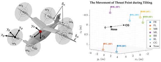
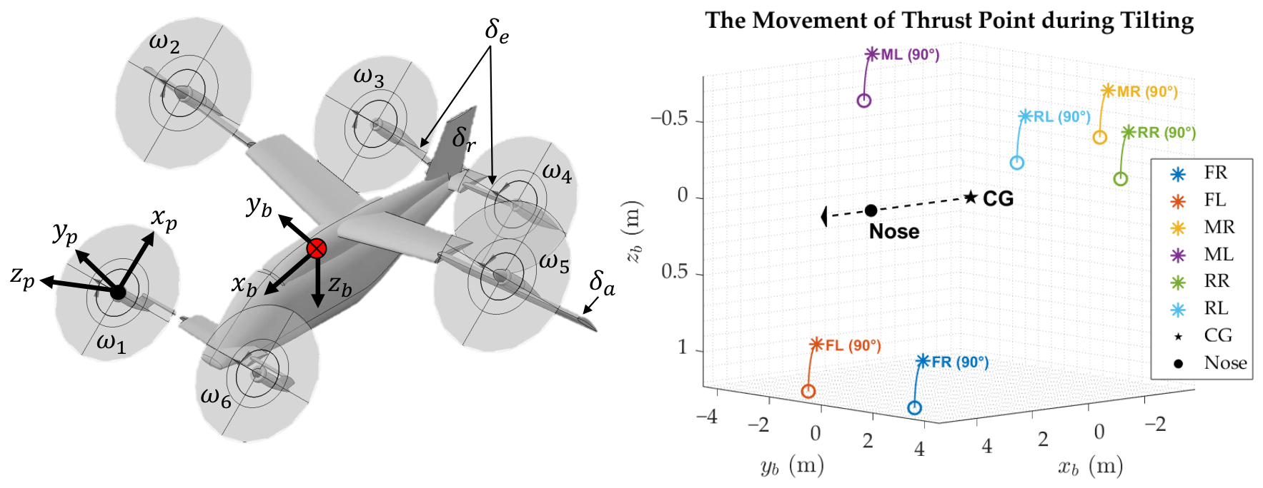
The tilt-wing configuration comprises a middle tilting wing for lift generation, a fore tilting wing for both lift generation and pitch moment generation in fixed-wing phase and an aft tilting wing that serves as the horizontal tail in fixed-wing phase. Figure 1 illustrates the reference body frame (with subscript ”b”) and propeller frame (with subscript ”p”).

Figure 1. Exemplary tilt-wing eVTOL in transition flight. The red dot marks the center of gravity (CG); the dashed line and arrow indicate the $x_b$ axis and its forward direction, respectively.

2.2. Flight Dynamics

The rigid-body dynamics model of the tilt-wing eVTOL is established in body frame.

$$\left\{\begin{array}{c}{\mathit{F}}_b=m\left({\displaystyle \frac{\delta {\mathit{V}}_b}{\delta t}}+{\mathit{\omega }}_b\times {\mathit{V}}_{\mathit{b}}\right)\hfill \\ {\mathit{M}}_b={\displaystyle \frac{\delta \mathit{h}}{\delta t}}+{\mathit{\omega }}_b\times \mathit{h}\hfill \end{array}\right.$$

(1)

where m is the mass of eVTOL, ${\mathit{V}}_b={\left[u_b{v}_b{w}_b\right]}^{\mathrm{T}}$ is the velocity components, ${\mathit{\omega }}_b={\left[pqr\right]}^{\mathrm{T}}$ is the angular rate components and $\mathit{h}=\int \mathit{r}\times ({\mathit{\omega }}_b\times \mathit{r})\mathrm{d}m$ denotes the angular momentum.

Ref. [33] focuses on a tilt-wing eVTOL with an aerodynamic configuration similar to the control subject of this paper, which provides the foundation of aerodynamic modelling for this study. The aerodynamic models for fixed-wing and multi-rotor phase are established by fitting CFD data:

$${\left[LCD\right]}^T=f\left(V_a,\alpha ,\overline{p},\overline{q},\overline{r},\beta ,{\omega }_p,{\delta }_{\mathrm{e}},{\delta }_{\mathrm{a}},{\delta }_{\mathrm{r}},{\delta }_{\mathrm{t}}\right)$$

(2)

$${\left[M_{ax}{M}_{ay}{M}_{az}\right]}^T=f\left(V_a,\alpha ,\overline{p},\overline{q},\overline{r},\beta ,{\omega }_p,{\delta }_{\mathrm{e}},{\delta }_{\mathrm{a}},{\delta }_{\mathrm{r}},{\delta }_{\mathrm{t}}\right)$$

(3)

where ${\left[LCD\right]}^T$ are aerodynamic lift, side force and drag. ${\left[M_{ax}{M}_{ay}{M}_{az}\right]}^T$ are aerodynamic roll moment, pitch moment and yaw moment. $M_{ay}$ is calculated about CG, located 3.56 m aft of the nose. For the fixed-wing configuration, corresponding to $\alpha =5^{\circ }$ level flight condition, the longitudinal static margin is 25% of the reference mean aerodynamic chord (MAC). The dominant parameters are airspeed $V_a$, angle of attack $\alpha$, sideslip angle $\beta$, non-dimensional angular rate $\overline{p},\overline{q},\overline{r}$, propeller rotational speed ${\omega }_p$, tilt angle ${\delta }_t$ and deflection of elevator ${\delta }_e$, aileron ${\delta }_a$ and rudder ${\delta }_r$.

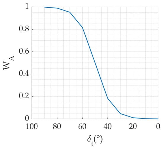
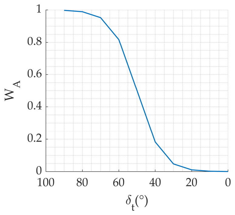
For transition(TR) aerodynamic mechanism, a hyperbolic-tangent-based blending function scheduling by ${\delta }_t$ is introduced to realize smooth transition between multi-rotor aerodynamics $C_{\mathrm{A},\mathrm{MR}}$ and fixed-wing aerodynamics $C_{\mathrm{A},\mathrm{FW}}$ [34]. ${\delta }_{t.\mathrm{MR}}={90}^{\circ },{\delta }_{t.\mathrm{FW}}=0^{\circ }$ are the start and end of blending. The transition aerodynamics $C_{\mathrm{A},\mathrm{TR}}$ is formulated as:

$$C_{\mathrm{A},\mathrm{TR}}=W_{\mathrm{A}}{C}_{\mathrm{A},\mathrm{MR}}+\left(1-W_{\mathrm{A}}\right)C_{\mathrm{A},\mathrm{FW}}$$

(4)

where

$$W_{\mathrm{A}}=1+{\displaystyle \frac{\tanh \left[k\left({\delta }_t-\overline{{\delta }_t}\right)\right]-1}{2}}$$

(5)

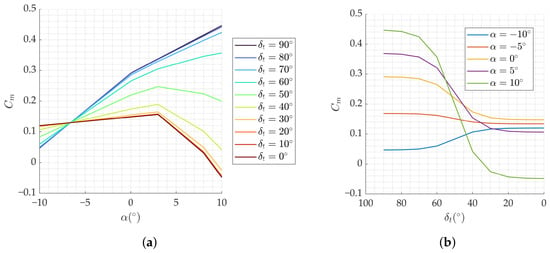
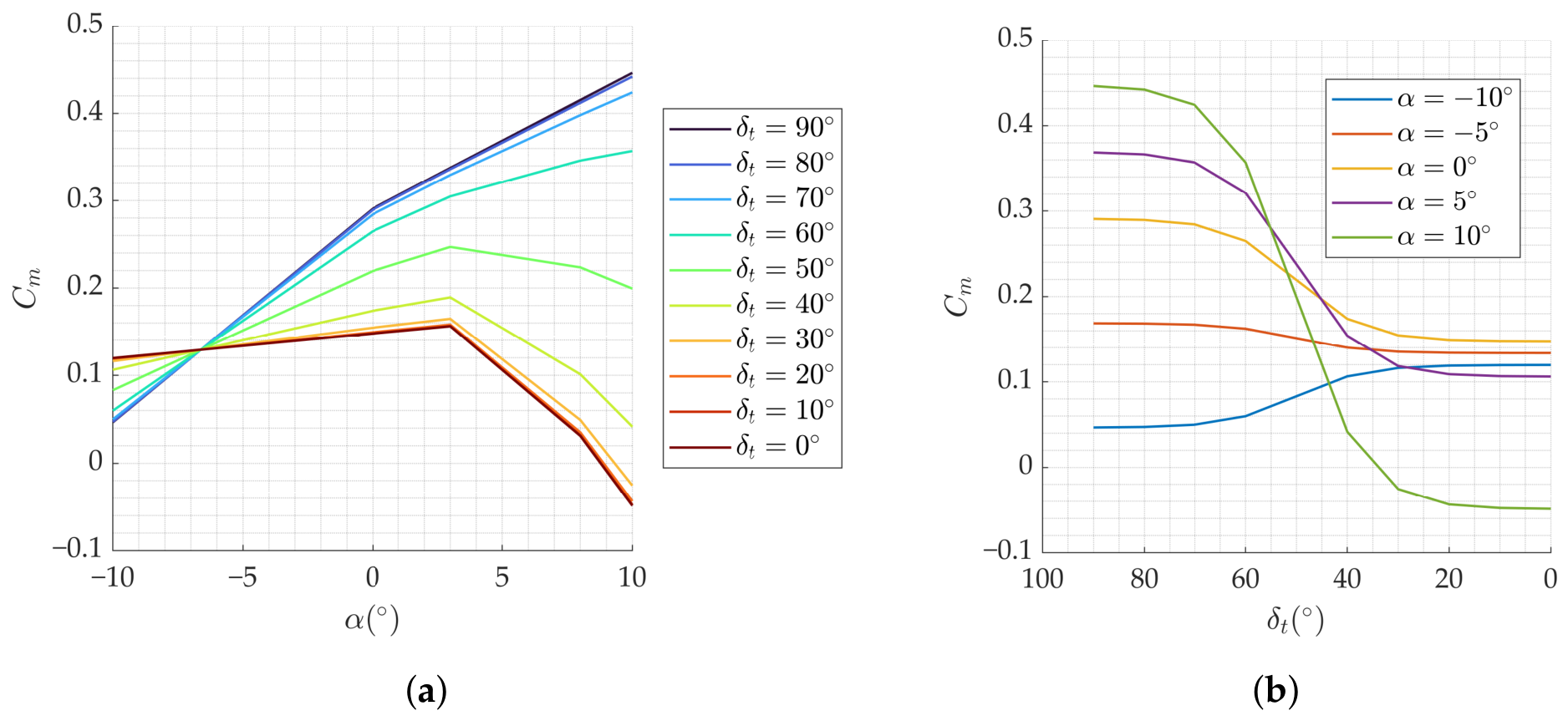
$W_{\mathrm{A}}$ represents the weight of multi-rotor aerodynamics, k controls the slope of $W_{\mathrm{A}}$ and $\overline{{\delta }_t}={\displaystyle \frac{{\delta }_{t.\mathrm{MR}}+{\delta }_{t.\mathrm{FW}}}{2}}$ controls the mid-point of blending function. Figure 2 shows the variation of $W_{\mathrm{A}}$ with ${\delta }_t$. Figure 3 shows $C_m$ variation with $\alpha$ and ${\delta }_t$.

Figure 2. Blending coefficient variation with tilt angle.

Figure 3. Transition aerodynamics: (a) Variation of $C_m$ with $\alpha$; (b) Variation of $C_m$ with ${\delta }_t$.

2.3. Electric-Propulsive Dynamics

The electric propulsion unit consists of the battery pack, electric motors, electronic speed controllers (ESC) and propellers, which jointly form an energy conversion chain from electrical power to propulsive force and moment. A component-level electric-propulsive dynamics model is adopted to represent the powertrain. For propeller aerodynamics, the quadratic form is adopted [35]. The thrust and torque coefficients $C_T,C_Q$ are dimensionless.

$$\left\{\begin{array}{c}{T}_p=\rho C_T{D_p}^4{\left({\displaystyle \frac{{\omega }_p}{2\pi }}\right)}^2\hfill \\ Q_p=\rho C_Q{D_p}^5{\left({\displaystyle \frac{{\omega }_p}{2\pi }}\right)}^2\hfill \end{array}\right.$$

(6)

where $T_p$ and $Q_p$ are the thrust and torque of single propeller in propeller frame, $D_p$ is the propeller diameter. The propulsive force and moment components are given by:

$$\left\{\begin{array}{c}{\displaystyle T_{xb}={\displaystyle \sum _i^{N_p}}{T}_{pi}\cos \left({\eta }_i+{\delta }_t\right)\cos {\chi }_i}\hfill \\ {\displaystyle T_{yb}={\displaystyle \sum _i^{N_p}}{T}_{pi}\sin {\chi }_i}\hfill \\ {\displaystyle T_{zb}=-{\displaystyle \sum _i^{N_p}}{T}_{pi}\sin \left({\eta }_i+{\delta }_t\right)\cos {\chi }_i}\hfill \end{array}\right.$$

(7)

$$\left\{\begin{array}{c}{\displaystyle M_{Tx}={\displaystyle \sum _i^{N_p}}\left[-T_{pi}(y_{Ti}\sin ({\eta }_i+{\delta }_t)\cos {\chi }_i+z_{Ti}\sin {\chi }_i)-{\sigma }_i{Q}_{pi}\cos ({\eta }_i+{\delta }_t)\cos {\chi }_i\right]}\hfill \\ {\displaystyle M_{Ty}={\displaystyle \sum _i^{N_p}}\left[T_{pi}(z_{Ti}\cos \left({\eta }_i+{\delta }_t\right)+x_{Ti}\sin \left({\eta }_i+{\delta }_t\right))\cos {\chi }_i-{\sigma }_i{Q}_{pi}\sin {\chi }_i\right]}\hfill \\ {\displaystyle M_{Tz}={\displaystyle \sum _i^{N_p}}\left[T_{pi}(x_{Ti}\sin {\chi }_i-y_{Ti}\cos \left({\eta }_i+{\delta }_t\right)\cos {\chi }_i)+{\sigma }_i{Q}_{pi}\sin ({\eta }_i+{\delta }_t)\cos {\chi }_i\right]}\hfill \end{array}\right.$$

(8)

where ${\delta }_t$ denotes tilt angle, defined as ${90}^{\circ }$ for vertically upward thrust and $0^{\circ }$ for horizontal forward thrust. $N_p$ is the number of propellers. $\eta$ is the longitudinal mounting angle measured from the positive $x_b$ axis toward the negative $z_b$ axis and $\chi$ is the lateral mounting angle measured from the $O{x}_b{z}_b$ plane toward the positive $y_b$ axis. ${\mathit{r}}_T={\left[x_{Ti}{y}_{Ti}{z}_{Ti}\right]}^{\mathrm{T}}$ contains the components of thrust lever arm vector and ${\sigma }_i=\pm 1$ is the rotational speed vector aligned with $\pm z_p$.

An equivalent circuit model (ECM) is used for electric characteristics [36]. ESC adjusts the motor terminal voltage by modulating the duty cycle $\upsilon$ according to the error between rotational speed command and the measured rotational speed. With input voltage, the motor generates current to balance the back electromotive force (BEMF) and provides torque.

$$\begin{array}{cc}\hfill U_M& =R_M{I}_M+K_E{\omega }_p={\displaystyle \frac{R_M{Q}_M}{K_T}}+K_E{\omega }_p\hfill \end{array}$$

(9)

$$\begin{array}{cc}\hfill {\dot{I}}_M& ={\displaystyle \frac{\upsilon U_B-R_M{I}_M-K_E{\omega }_M}{L_M}}\hfill \end{array}$$

(10)

$$\begin{array}{cc}\hfill {\dot{\omega }}_M& ={\displaystyle \frac{K_T{I}_M-Q_P}{J_S}}\hfill \end{array}$$

(11)

where $Q_M$ is the torque provided by motor, $J_S$ is motor-propeller shaft inertia, $\upsilon$ is duty cycle, $I_M$ is the current of motor, $U_M$ is the terminal voltage of motor, $R_M$ is the internal resistance of motor and $K_E,K_T$ are respectively the back electromotive force and torque constant. For steady case analysis, the dynamic characteristics of motor response are neglected which leads to ${\dot{I}}_M=0,{\dot{\omega }}_M=0$. Moreover, neglect the transmission power loss from motor to propeller, which yields ${\omega }_P={\omega }_M$ [20].

The battery pack is modeled as $N_{bp}$ parallel strings, each containing $N_{bs}$ cells in series. The terminal voltage of the battery pack can be expressed as:

$$U_B=N_{bs}{U}_{OC}-{\displaystyle \frac{N_{bs}}{N_{bp}}}{R}_B{I}_B$$

(12)

where $I_B$ is the current of battery pack, and $R_B$ is the internal resistance of a single battery cell. The formulation without polarization voltage state is adopted for open-circuit voltage [37]:

$$U_{OC}={\beta }_1\ln \left(\mathrm{SOC}\right)+\exp \left({\beta }_2\mathrm{SOC}\right)+{\beta }_3{\mathrm{SOC}}^3+{\beta }_4$$

(13)

Following prior work in ref. [20], the battery open-circuit voltage coefficients ${\beta }_1,{\beta }_2,{\beta }_3,{\beta }_4$ are determined by least squares fitting to published lithium-ion battery discharge characteristics. Such data can be obtained using the eight-channel charge–discharge experimental procedure reported in ref. [37]. $SOC=1-{\displaystyle \frac{Q_B}{Q_{Bmax}}}$ represents the remaining charge of the battery pack. The rate of change of battery charge is defined as:

$${\dot{Q}}_B={\displaystyle \frac{I_B}{3600}}$$

(14)

3. Corridor-Protected Methodology

3.1. Transition Corridor and Protection Boundaries

The transition corridor represents an admissible set of flight states, in which eVTOLs can achieve speed and configuration transformation under specific constraints [8]. Specifically, the state boundaries for protection are lower-dimensional limit surfaces extracted from the multi-dimensional transition corridor and serve as protection boundaries.

3.1.1. Constraints for Transition Corridor

Physical constraints arise from the requirements of flight and control. Flight constraints are mission-dependent, whereas control constraints are hard physical limits of the aircraft.

(a)

Flight Constraints

In this study, transition feasibility is evaluated under nominal level-flight conditions using the following longitudinal quasi-equilibrium equations:

$$\left\{\begin{array}{c}{\displaystyle m\dot{V}={\displaystyle \sum _i^{N_p}}{T}_{pi}\cos \left(\alpha +{\eta }_i+{\delta }_t\right)-C_D\left(\alpha ,{\delta }_t\right)\overline{q}{S}_R-mg\sin \gamma }\hfill \\ {\displaystyle mV\dot{\gamma }={\displaystyle \sum _i^{N_p}}{T}_{pi}\sin \left(\alpha +{\eta }_i+{\delta }_t\right)+C_L\left(\alpha ,{\delta }_t\right)\overline{q}{S}_R-mg\cos \gamma ⩾0}\hfill \\ {\displaystyle I_{yy}\dot{q}={\displaystyle \sum _i^{N_p}}{T}_{pi}\left[z_{Ti}\cos \left({\eta }_i+{\delta }_t\right)+x_{Ti}\sin \left({\eta }_i+{\delta }_t\right)\right]+C_M\left(\alpha ,{\delta }_t,{\delta }_e\right)\overline{q}{S}_R{c}_R=0}\hfill \end{array}\right.$$

(15)

where $\gamma$ is the flight path angle, $S_R$ is the aerodynamic reference area and $\overline{q}=0.5\rho V^2$ denotes the dynamic pressure at current altitude. $\dot{\gamma }⩾0$ is required to allow upward flight path tendency. $\dot{q}=0$ assures pitch attitude equilibrium.

(b)

Control Constraints

Control constraints mainly arise from aerodynamic stability and electric-propulsion capability. Aerodynamic constraint is imposed on the effective angle of attack arising from the stall limit [38] during transition.

$$\alpha ⩽{\alpha }_{\mathrm{stall}}$$

(16)

where ${\alpha }_{\mathrm{stall}}$ is the critical angle of attack when the wing or elevator enters a region of significant flow separation. Propeller aerodynamic constraint is imposed on the maximum blade-tip Mach number, which contributes to avoiding substantial aerodynamic efficiency losses associated with compressibility effects. $M_{tip}$ for check is determined from the maximum resultant velocity of the freestream flow and blade-tip rotation [39].

$$M_{tip}={\displaystyle \frac{1}{a}}\sqrt{V_{\infty }^2+{\left({\displaystyle \frac{{\omega }_p{D}_p}{2}}\right)}^2+V_{\infty }{\omega }_p{D}_p\sin {\beta }_p}<M_{\max }$$

(17)

where a is the speed of sound at current flight altitude, $V_{\infty }$ is the true airspeed. ${\beta }_p={\delta }_t+\alpha +\eta$ denotes the angle between the propeller axis and $V_{\infty }$ direction. According to ref. [40], a maximum helical tip Mach number of $M_{\max }=0.85$ is adopted as a preliminary screening threshold for propellers of DEP layout. This reference value is close to the critical Mach number of commonly used airfoils but can be adjusted according to the actual propeller characteristics. Propulsion constraints are jointly determined by battery and motor [20]:

$$\begin{array}{cc}\hfill I_B& ={\displaystyle \frac{N_{bp}\left(N_{bs}{U}_{OC}-\sqrt{{\left(N_{bs}{U}_{OC}\right)}^2-\frac{4R_B{N}_{bs}}{N_{bp}}{P}_M}\right)}{2R_B{N}_{bs}}}\in \left[0,I_{B\max }\right]\hfill \end{array}$$

(18)

$$\begin{array}{cc}\hfill P_M& ={\displaystyle \sum _i^{N_p}}{P}_{Mi}={\displaystyle \sum _i^{N_p}}\left[{\displaystyle \frac{Q_{Mi}}{K_T}}\left({\displaystyle \frac{R_M{Q}_{Mi}}{K_T}}+K_E{\omega }_{pi}\right)\right]⩽P_{M\max }\hfill \end{array}$$

(19)

Actuator constraint $\left|{\delta }_e\right|⩽{\delta }_{e\max }$ is also inviolable.

3.1.2. Transition Corridor Construction

Based on the above constraints, the transition corridor is constructed in three dimensions of tilt angle, forward velocity and angle of attack. Within the candidate state domain $\mathcal{D}\subseteq {\mathbb{R}}^3$, defined by $({\delta }_t,V,\alpha )$, a state is retained as feasible only when all aerodynamic, electric and propulsion constraints are simultaneously satisfied. The feasible regions for transition and retransition are denoted by ${\mathcal{C}}_F,{\mathcal{C}}_R$, respectively.

$$\begin{array}{c}\hfill {\mathcal{C}}_F=\left\{({\delta }_t,V,\alpha )\in \mathcal{D}\left|\dot{V}>0,\dot{\gamma }⩾0,\dot{q}=0,g_j\left({\delta }_t,V,\alpha \right)⩽0,\forall j\right.\right\}\end{array}$$

(20)

$$\begin{array}{c}\hfill {\mathcal{C}}_R=\left\{({\delta }_t,V,\alpha )\in \mathcal{D}\left|\dot{V}<0,\dot{\gamma }⩾0,\dot{q}=0,g_j\left({\delta }_t,V,\alpha \right)⩽0,\forall j\right.\right\}\end{array}$$

(21)

where $\dot{V}$ denotes the forward acceleration, which is required to be positive in forward transition and negative in backward transition. Under $\gamma =0$ initial condition, the constraint $\dot{\gamma }⩾0$ corresponds to nonnegative vertical acceleration. $g_j$ denotes the j-th constraint defined in the last section. In order to obtain ${\mathcal{C}}_F,{\mathcal{C}}_R$, a cascaded longitudinal trim procedure is employed.

For each prescribed ${\delta }_t,V,\alpha$, the aerodynamic forces and pitching moment are determined. A redistributed pseudoinverse approach with set enumeration is adopted. First, the admissible total thrust range $[T_{\Sigma ,\mathrm{lo}},T_{\Sigma ,\mathrm{hi}}]$ is determined from the force and moment equilibrium, with elevator deflection adjusted when necessary. The required total thrust $T_{\Sigma }={\sum }_{i=1}^{N_p}{T}_i$ is then set to $T_{\Sigma ,\mathrm{lo}}$. If $T_{\Sigma ,\mathrm{lo}}>T_{\Sigma ,\mathrm{hi}}$, the candidate is rejected. Candidates with inconsistent thrust bounds or unsatisfied equilibrium requirements are also reported infeasible. The Moore–Penrose pseudo inverse is employed to obtain an initial minimum norm solution [41] satisfying both the total thrust and pitching moment equilibrium requirements:

$${\mathit{T}}^0={\mathit{A}}^{\mathit{T}}{\left({\mathit{AA}}^{\mathit{T}}\right)}^{-1}\mathit{b}$$

(22)

For longitudinal thrust allocation on the investigated configuration, the left and right propellers within each group are assumed to generate equal thrust, thus the $N_p=6$ propellers can be divided into the front, middle and rear groups for bounded redistribution. The three groups of propellers have distinct pitching moment effectiveness coefficients, indicating that the initial effectiveness matrix $\mathit{A}$ has full row rank.

$$\begin{array}{cc}\hfill \mathit{A}& =\left[\begin{array}{ccc}1& 1& 1\\ l_1& l_2& l_3\end{array}\right]\hfill \end{array}$$

(23)

$$\begin{array}{cc}\hfill \mathit{b}& =\left[\begin{array}{c}{T}_{\Sigma }\\ -C_M({\delta }_t,\alpha ,{\delta }_e)\overline{q}{S}_R{c}_R\end{array}\right]\hfill \end{array}$$

(24)

where $l_i=\left[z_{Ti}\cos \left({\eta }_i+{\delta }_t\right)+x_{Ti}\sin \left({\eta }_i+{\delta }_t\right)\right]$ is the derivative of pitch moment with respect to each group of thrust direction. If the initial allocation violates the thrust bounds, six additional combinations are examined by fixing one of the thrust groups at either zero or its maximum allowable value and redistributing the remaining demand using Equation (25). The feasible solution with the minimum norm of thrusts is selected.

$${\mathit{T}}_f={\mathit{A}}_f^{-1}\left(\mathit{b}-{\mathit{A}}_s{\mathit{T}}_s\right)$$

(25)

where ${\mathit{T}}_f$ and ${\mathit{T}}_s$ denote the thrust of the free and fixed propeller groups, respectively. ${\mathit{A}}_f$ and ${\mathit{A}}_s$ are the corresponding effective matrices. The term $(\mathit{b}-{\mathit{A}}_s{\mathit{T}}_s)$ represents the residual force and pitching moment demands to be allocated.

During bounded redistribution, the reduced allocation matrix ${\mathit{A}}_f$ is nonsingular when the remaining groups have distinct pitching moment effectiveness coefficients. Cases with only one free group are excluded during transition and handled separately in fixed-wing flight, where thrust is determined from force equilibrium and pitching moment is balanced primarily through elevator adjustment. Finally, all feasible states ${\mathit{T}}^{*}={\left[{\mathit{T}}_f{\mathit{T}}_s\right]}^{\mathrm{T}}$ satisfying electrical constraints form the transition corridor ${\mathcal{C}}_F$ and retransition corridor ${\mathcal{C}}_R$.

Every state within the intersection of ${\mathcal{C}}_F$ and ${\mathcal{C}}_R$ possesses both acceleration and deceleration capability under the prescribed constraints, providing a basis for flexible forward speed adjustment. This intersection serves for protection boundaries generation:

$$\mathcal{C}={\mathcal{C}}_F\cap {\mathcal{C}}_R$$

(26)

3.1.3. Variables Generation for Protection Boundaries

Protection boundaries are contracted based on $\partial \mathcal{C}$. For longitudinal flight, the pitch angle satisfies $\theta =\alpha +\gamma$. Under the nominal level-flight condition $\gamma =0$, this relation leads to the $\theta =\alpha$ assumption [42]. Accordingly, the ${\mathcal{C}}_{\alpha }$ boundary constructed by the corridor prediction is mapped to pitch limits. A prescribed $1^{\circ }$ safety margin is adopted to reduce the risk of exceeding pitch boundary. The margin selection considers both stall risk and pitch measurement uncertainty, with reference to the $\alpha$ margin in [42] and the reported pitch accuracy of a commercial attitude and heading reference system (AHRS) in [43]. It can be adjusted according to actual system requirements.

$${\theta }_{\lim \pm }={\mathcal{C}}_{\alpha }\mp 1^{\circ }=f(V,{\delta }_t)$$

(27)

At each state $({\delta }_t,V,\alpha )$, the maneuverability boundary is defined as the maximum pitch angular accelerations at current state, which are determined by residual propulsive and aerodynamic control sources beyond the equilibrium requirement. Assume that initial rates are zero, and the angular accelerations are calculated by rotational dynamics. Different from conventional airplanes, $I_{xz}$ is often non-negligible for eVTOL.

$$\left[\begin{array}{c}\dot{p}\\ \dot{q}\\ \dot{r}\end{array}\right]={\left[\begin{array}{ccc}{I}_{xx}& 0& -I_{xz}\\ 0& I_{yy}& 0\\ -I_{xz}& 0& I_{zz}\end{array}\right]}^{-1}\left[\begin{array}{c}{M}_{Tx}+M_{ax}\\ M_{Ty}+M_{ay}\\ M_{Tz}+M_{az}\end{array}\right]$$

(28)

In order to obtain the attainable $\dot{q}$ as maneuverability boundaries ${\dot{q}}_{max\pm }=f({\delta }_t,V,\alpha ,{\delta }_e)$, a constrained nonlinear optimization problem is constructed as Equation (29). The optimization decision variables are the normalized squared propeller rotational speeds defined as $z_i={\omega }_{pi}^2/{\omega }_{p\max }^2$, to improve numerical scaling. The optimization is subject to forces and moments constraints and propulsion and electrical constraints. The aerodynamic pitching moment is precomputed at 80% maximum elevator deflection. For each optimization, the candidate providing the most favorable pitching moment is selected and held fixed during optimization.

$$\begin{array}{cc}\hfill \underset{\mathit{z}}{\text{Max/Min}}& \dot{q}\hfill \\ \hfill \mathrm{s}.\mathrm{t}.& {\displaystyle \sum _i^{N_p}}{T}_{pi}\left({\omega }_{pi}\right)\cos \left({\delta }_t+\alpha +{\eta }_i\right)-0.5\rho V^2{S}_R{C}_D\left({\delta }_t,\alpha \right)-mg\sin \gamma ⩾0\left(\mathrm{TR}\right),⩽0\left(\mathrm{RT}\right)\hfill \\ \hfill & {\displaystyle \sum _i^{N_p}}{T}_{pi}\left({\omega }_{pi}\right)\sin \left({\delta }_t+\alpha +{\eta }_i\right)+0.5\rho V^2{S}_R{C}_L\left({\delta }_t,\alpha \right)-mg\cos \gamma ⩾0\hfill \\ \hfill & M_{Tx}\left({\mathit{\omega }}_{\mathit{p}}\right)+M_{ax}\left({\mathit{\omega }}_{\mathit{p}}\right)=0,M_{Tz}\left({\mathit{\omega }}_{\mathit{p}}\right)+M_{az}\left({\mathit{\omega }}_{\mathit{p}}\right)=0\hfill \\ \hfill & P_M\left({\omega }_{pi}\right)⩽P_{M\max },M_{tip}\left({\omega }_{pi}\right)⩽M_{tip\max }\hfill \\ \hfill & I_B\left({\mathit{\omega }}_{\mathit{p}}\right)⩽I_{B\max }\hfill \\ \hfill & 0⩽z_i⩽1,i=1,\dots ,N_p\hfill \end{array}$$

(29)

Subsequently, the maximum and minimum pitch angular acceleration are determined separately for each axis, subject to the propeller speed limits and the prescribed flight, electrical and propulsion constraints. The optimization problem is solved using a sequential quadratic programming (SQP) algorithm implemented in MATLAB R2023b.

The ${\theta }_{\lim \pm }$ and ${\dot{q}}_{\max \pm }$ are both precomputed offline.

3.2. Protected Control Strategy

The protection boundaries above are used for command limit. The pitch control command ${\theta }_c$ should satisfy:

$${\theta }_c=\left\{\begin{array}{cc}{\theta }_{\lim -},\hfill & {\theta }_{c0}⩽{\theta }_{\lim -}\hfill \\ {\theta }_{c0},\hfill & {\theta }_{\lim -}<{\theta }_{c0}<{\theta }_{\lim +}\hfill \\ {\theta }_{\lim +},\hfill & {\theta }_{c0}⩾{\theta }_{\lim +}\hfill \end{array}\right.$$

(30)

where ${\theta }_{c0}$ denotes the raw control command input by pilot, ${\theta }_{\lim -}$ and ${\theta }_{\lim +}$ denote the nose-down and nose-up pitch command limit defined by Equation (27).

For inner-loop rate limiting, this paper proposes a maneuverability-based (MB) dynamic protection method. First is the formulation of $q_{\lim }$ and corresponding ${\dot{q}}_{\lim }$. In order to ensure $\theta ⩽{\theta }_{\lim }$, pitch rate should approach zero simultaneously when $\theta \to {\theta }_{\lim }$. As $\theta$ approaches ${\theta }_{\lim }$, the decay rate of q should be determined with reference to the maximum attainable pitch acceleration ${\dot{q}}_{\max }$ obtained from trim analysis. Define $q_{\lim }$ as the maximum recoverable rate, which is the final boundary where eVTOL is still capable of recovering the pitch angle onto its safe region:

$$\left\{\begin{array}{c}{q}_{\lim -}=-\sqrt{2{\dot{q}}_{\max +}(\theta -{\theta }_{\lim -})}\hfill \\ q_{\lim +}=\sqrt{2(-{\dot{q}}_{\max -})({\theta }_{\lim +}-\theta )}\hfill \end{array}\right.$$

(31)

where ${\dot{q}}_{\max +}⩾0$ and ${\dot{q}}_{\max -}⩽0$ are respectively the maximum nose-up and nose-down pitch angular acceleration. $q_{\lim -}⩽0$ is the pitch rate limit when pitch angle approaches its negative boundary. $q_{\lim +}⩾0$ is the pitch rate limit when pitch angle approaches its positive boundary. Both $q_{\lim -}$ and $q_{\lim +}$ become zero when pitch angle reaches the limit. At the critical margin of $\theta$, $q_{\lim }\to 0$. Take the positive pitching motion as an example. At a certain $\theta$, the safety margin of pitch rate is:

$$h_{+}=q_{\lim +}^2-q^2=-2{\dot{q}}_{\max -}({\theta }_{\lim +}-\theta )-q^2$$

(32)

When $h_{+}⩾0$, $\left|q\right|⩽q_{\lim +}$ must hold. Following the level-flight assumption, we neglect the cross-coupling effects of roll angle and yaw rate on the pitch angle rate in current analysis, which leads to $\dot{\theta }=q$. Moreover, based on the instantaneous maneuverability, the pitch boundary and available opposing angular acceleration are assumed constant at the current state. Under the above assumptions, if $\dot{q}$ is allowed to reach ${\dot{q}}_{\max -}$ at the critical margin $h_{+}=0$, the safety function derivative can be derived as:

$${\dot{h}}_{+}=2{\dot{q}}_{\max -}q-2q\dot{q}=0$$

(33)

This implies that, theoretically, if available opposing pitch acceleration is applied, the pitch rate can be reduced to zero exactly at ${\theta }_{\lim +}$. The derivative of the pitch rate limit is:

$${\dot{q}}_{\lim +}={\displaystyle \frac{d{q}_{\lim +}}{d\theta }}\dot{\theta }={\displaystyle \frac{{\dot{q}}_{max-}}{q_{\lim +}}}q$$

(34)

To avoid singularity of $q_{\lim }\to 0$, introduce a small threshold in the denominator. Feedback control is required to guarantee that q stays below $q_{\lim +}$. Take the upper case as an example, the error between q and $q_{\lim +}$ should satisfy:

$$e_{q+}=q_{\lim +}-q⩾0$$

(35)

Design the limit of ${\dot{q}}_{cmd}$ as

$${\dot{q}}_{cmd}⩽{\dot{q}}_{\lim +}+K_{q.\mathrm{protect}}(q_{\lim +}-q)$$

(36)

This saturation law contributes to guaranteeing $e_{q+}⩾0$. Assume an error expression as:

$${\dot{e}}_{q+}={\dot{q}}_{\lim +}-\dot{q}⩾-K_q{e}_{q+}$$

(37)

At the bound where ${\dot{e}}_{q+}=-K_q{e}_{q+}$, the analytical solution is:

$$e_{q+}\left(t\right)=e_{q+}\left(0\right)e^{-K_{q}t}$$

(38)

where $K_q$ is defined to be positive. As the aircraft will not initiate flight with a boundary-exceed rate, $e_{q+}\left(0\right)⩾0$ always holds in practice. Thus, $e_{q+}⩾0$ is theoretically maintained under ideal angular acceleration tracking and an initially admissible pitch rate.

4. Controller Implementation

4.1. Unified Controller Structure

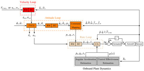
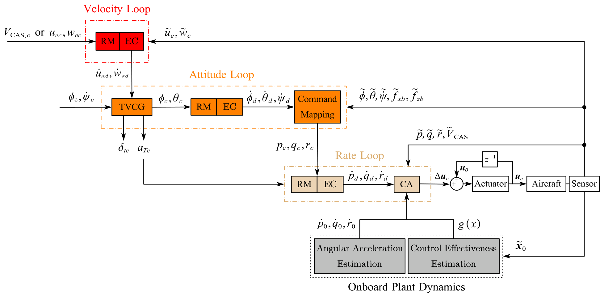
The multi-loop unified INDI controller structure is demonstrated in Figure 4. The velocity loop consists of reference model (RM) and error controller (EC). The attitude loop aims to enhance attitude stability, incorporating thrust vector command generation (TVCG). The inner loop aims to enhance damping, incorporating control allocation (CA). Through time-scale separation, the design of each loop becomes a dynamic-inversion problem for a first-order system, which simplifies the computation and enhances robustness.

Figure 4. Multi-loop unified controller structure.

4.2. Control Command

In multi-rotor flight, powered-lift dominates the control authority, making precise hovering control the primary handling requirement [44]. Therefore, translational rate commands are adopted for vertical and horizontal motion. In fixed-wing flight, aerodynamics dominate and the flight path is mainly changed indirectly through attitude-induced aerodynamic forces. Thus, attitude-hold commands are adopted [45]. In transition, smoothness assurance and stability augmentation are more important than precise position control so the attitude commands are retained. Considering the limitations of airspeed signal at low speeds, ground speed is adopted as the speed-channel command [44]. The heading rate response type is adopted for all phases.

The unified control commands are summarized in Table 1.

Table 1. Control commands.

Flight Phase	Throttle	Longitudinal	Lateral	Yaw
Multi-rotor	$u_e$	$w_e$	$\varphi$	$\dot{\psi }$
Transition	$u_e$
Fixed-wing	$V_{\mathrm{CAS}}$	$\theta$
Retransition	$u_e$

4.3. Thrust Vector Command Generation

The desired translational motion is converted into thrust vector command, including the thrust orientation command ${\delta }_{tc}, {\theta }_c$ and thrust magnitude command $a_{Tc}$.

${\delta }_{tc}$ is defined to be ${90}^{\circ }$ and $0^{\circ }$ for multi-rotor phase and fixed-wing phase. In transition phase, ${\delta }_{tc}$ is scheduled by forward velocity command according to predefined flight path.

${\theta }_c$ is mapped from the desired accelerations utilizing longitudinal translational dynamics in multi-rotor phase [46], yielding

$$\left[\begin{array}{c}{\dot{u}}_{ed}\\ {\dot{w}}_{ed}\end{array}\right]={\displaystyle \frac{1}{m}}\left[\begin{array}{cc}\cos \theta & \cos \varphi \sin \theta \\ -\sin \theta & \cos \varphi \cos \theta \end{array}\right]\left[\begin{array}{c}{T}_{xb}\\ T_{zb}\end{array}\right]+\left[\begin{array}{c}0\\ g\end{array}\right]-\left[\begin{array}{c}-\dot{\psi }{v}_e\\ 0\end{array}\right]$$

(39)

The subscript ”e” herein denotes the control frame defined in ref. [46], obtained by rotating the local North–East–Down (NED) frame through the aircraft heading angle. Let ${\left[f_{xb}{f}_{zb}\right]}^{\mathrm{T}}={\displaystyle \frac{{\left[T_{xb}{T}_{zb}\right]}^{\mathrm{T}}}{m}}$ denote the propulsive specific forces in the body frame. ${\theta }_c$ can be obtained from Equation (39):

$${\theta }_c=\mathrm{atan}{\displaystyle \frac{f_{zb}\cos {\varphi }_{c}K-f_{xb}}{f_{zb}\cos {\varphi }_c+f_{xb}K}}$$

(40)

where $K={\displaystyle \frac{{\dot{u}}_{ed}-\dot{\psi }{v}_e}{{\dot{w}}_{ed}-g}}$. This transformation achieves the thrust distribution based on the force required for acceleration and the force required for altitude maintenance. There are two focuses:

(a)

During hovering, the numerator approaches zero and causes an artificial $\pm \pi$ jump.

(b)

During vertical take-off, K becomes singular when ${\dot{w}}_{ed}=g$.

Therefore, tangent branch selection and singularity protection are required. In transition phase, predefined pitch profile is adopted as ${\theta }_c$. In fixed-wing phase, ${\theta }_c$ comes from manual input.

The acceleration in the thrust direction can serve as the thrust magnitude command $a_{Tc}$, being calculated from velocity command, $\theta$ and ${\delta }_t$.

$$a_{Tc}=\mathsf{\Delta }{\dot{u}}_{ec}\cos \left(\theta +{\delta }_t\right)-\mathsf{\Delta }{\dot{w}}_{ec}\sin \left(\theta +{\delta }_t\right)$$

(41)

4.4. Reference Model

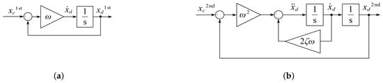
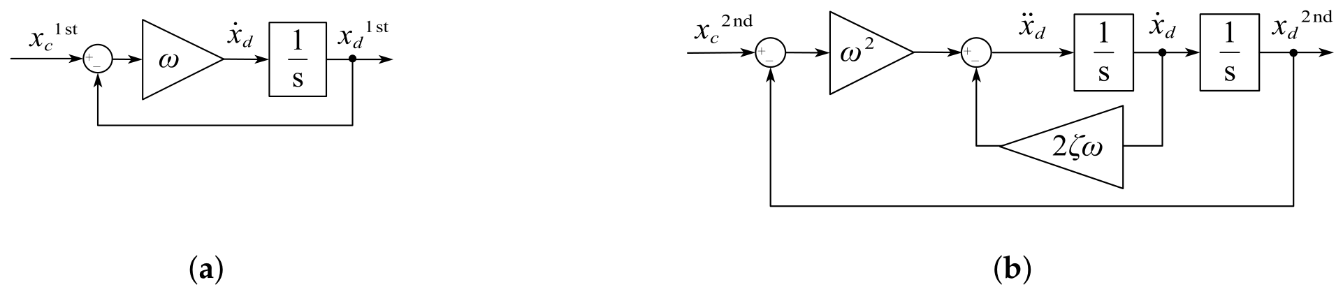
Figure 5 shows the structure of reference models. Define the state variables with desired first-order response characteristics as $x_c^{1\mathrm{st}}={\left[{\varphi }_c{\dot{\psi }}_c{u}_{ec}{w}_{ec}{p}_c{q}_c{r}_c\right]}^{\mathrm{T}}$ and the state variables with desired second-order response characteristics as $x_c^{2\mathrm{nd}}={\theta }_c$ [47].

Figure 5. Reference model structure: (a) 1st Reference Model; (b) 2nd Reference Model.

For velocity loop, the response of translational rates to thrust corresponds to first-order characteristics [46]. The pseudo input for attitude loop is:

$$v=\left[\begin{array}{c}{\dot{u}}_{ed}\\ {\dot{w}}_{ed}\end{array}\right]=\left[\begin{array}{c}{\omega }_u\left(u_{ec}-u_{ed}\right)\\ {\omega }_w\left(w_{ec}-w_{ed}\right)\end{array}\right]$$

(42)

where ${\omega }_u$ and ${\omega }_w$ denote the bandwidth of forward and vertical velocity. Internal states of the reference model are denoted with subscript d. According to the translational rate response requirements in ADS-33E-PRF [48], the expected bandwidths are selected within 0.2 rad/s–0.4 rad/s.

For attitude loop, the responses of roll angle and yaw rate to actuators correspond to first-order characteristics and the response of pitch angle corresponds to the second relative order [46]. The selection of bandwidth and damping of attitude loop ${\omega }_{\varphi },{\omega }_{\theta },{\zeta }_{\theta },{\omega }_{\dot{\psi }}$ is related to desired modal characteristics, which are selected with reference to the Level 1 requirements for Class I aircraft in Category C [48,49].

$${\mathit{\nu }}_{\mathrm{Att}}=\left[\begin{array}{c}{\dot{\varphi }}_d\\ {\dot{\theta }}_d\\ {\dot{\psi }}_d\end{array}\right]=\left[\begin{array}{c}{\omega }_{\varphi }({\varphi }_c-{\varphi }_d)\\ {\displaystyle \frac{{\omega }_{\theta }^2({\theta }_c-{\theta }_d)-{\ddot{\theta }}_d}{2{\zeta }_{\theta }{\omega }_{\theta }}}\\ {\dot{\psi }}_d\end{array}\right]$$

(43)

The desired yaw rate is generated by a first-order reference model ${\ddot{\psi }}_d={\omega }_{\dot{\psi }}({\dot{\psi }}_c-{\dot{\psi }}_d)$. Utilizing rotational kinematics inversion to map ${\mathit{\nu }}_{\mathrm{Att}}$ to the inputs of inner loop [44]:

$$u_{\mathrm{c},Inner}=\left[\begin{array}{c}{p}_c\\ q_c\\ r_c\end{array}\right]=B_{0,\mathrm{Att}}^{-1}{\mathit{\nu }}_{\mathrm{Att}}$$

(44)

The control matrix is

$$B_{0,\mathrm{Att}}={\displaystyle \frac{\partial g(x,u)}{\partial u}}=\left[\begin{array}{ccc}1& \sin \left(\varphi \right)\tan \left(\theta \right)& \cos \left(\varphi \right)\tan \left(\theta \right)\\ 0& \cos \left(\varphi \right)& -\sin \left(\varphi \right)\\ 0& {\displaystyle \frac{\sin \left(\varphi \right)}{\cos \left(\theta \right)}}& {\displaystyle \frac{\cos \left(\varphi \right)}{\cos \left(\theta \right)}}\end{array}\right]$$

(45)

For inner loop, the relative degree of angular rates exists as first-order. The pseudo commands for control allocation are:

$${\mathit{\nu }}_{\mathrm{Rate}}=\left[\begin{array}{c}{\dot{p}}_d\\ {\dot{q}}_d\\ {\dot{r}}_d\end{array}\right]=\left[\begin{array}{c}{\omega }_p(p_c-p_d)\\ {\omega }_q(q_c-q_d)\\ {\omega }_r(r_c-r_d)\end{array}\right]$$

(46)

Inner loop bandwidths ${\omega }_p,{\omega }_q,{\omega }_r$ are also determined by the modal requirements above. Above all, the pseudo input for control allocation is:

$${\mathit{\nu }}_{\mathrm{Inner}}={\left[a_{Tc}{\dot{p}}_d{\dot{q}}_d{\dot{r}}_d\right]}^{\mathrm{T}}$$

(47)

4.5. Control Allocation

Control allocation undertakes the task of coordinating allocation strategies for different flight phases. ${\mathit{\nu }}_{\mathrm{Rate}}$ control is primarily realized by propellers in multi-rotor phase, aerodynamic surfaces in fixed-wing phase and their combination during transition. $a_{Tc}$ relies on propellers in all phases, yet only a subset of designated propellers is activated in fixed-wing phase for energy saving. Hence, a selection strategy is incorporated into the allocation.

First, ${\mathit{\nu }}_{\mathrm{Rate}}$ is partitioned by airspeed into contributions from propellers and surfaces. Define $V_T,V_A$ as the start and end of blending from powered control to aerodynamic control.

$${\mathit{\nu }}_{\mathrm{Rate}}={\mathit{\nu }}_{\omega ,\mathrm{Rate}}+{\mathit{\nu }}_{\delta ,\mathrm{Rate}}=\lambda {\mathit{\nu }}_{Rate}+\left(1-\lambda \right){\mathit{\nu }}_{Rate}$$

(48)

where

$$\lambda =1-k_{\lambda }\overline{V}+(k_{\lambda }-1){\overline{V}}^2,\overline{V}={\displaystyle \frac{V-V_T}{V_A-V_T}}$$

(49)

$\lambda$ represents the thrust-borne control authority, which decreases as dynamic pressure increases [5]. $k_{\lambda }=0-1$ controls the shape of blending function. When $k_{\lambda }=1$, the blending function degenerates from quadratic to linear.

Second, ${\mathit{\nu }}_{\delta ,\mathrm{Rate}}$ and ${\mathit{\nu }}_{\omega ,\mathrm{Rate}}$ are allocated based on INDI. For surface allocation,

$$\mathsf{\Delta }{\delta }_c={\delta }_c-{\delta }_0={B_{0,\mathrm{Rate}}}^{-1}({\mathit{\nu }}_{\delta ,\mathrm{Rate}}-{\dot{\mathsf{\Omega }}}_0)$$

(50)

where $\delta$ denotes the control surface deflections, including ${\delta }_a$, ${\delta }_e$ and ${\delta }_r$. ${\delta }_0,{\mathsf{\Omega }}_0$ respectively denote the current surfaces deflection and rates. $B_{0,\mathrm{Rate}}$ is the control allocation matrix, which is obtained by an onboard plant model. Using differences instead of derivatives to accommodate discrete computation [50].

$$B_{0,\mathrm{Rate}}={\displaystyle \frac{\partial g(x,u)}{\partial u}}=\left[\begin{array}{ccc}{\displaystyle \frac{\partial \dot{p}}{\partial {\delta }_{\mathrm{a}}}}& {\displaystyle \frac{\partial \dot{p}}{\partial {\delta }_{\mathrm{e}}}}& {\displaystyle \frac{\partial \dot{p}}{\partial {\delta }_{\mathrm{r}}}}\\ {\displaystyle \frac{\partial \dot{q}}{\partial {\delta }_{\mathrm{a}}}}& {\displaystyle \frac{\partial \dot{q}}{\partial {\delta }_{\mathrm{e}}}}& {\displaystyle \frac{\partial \dot{q}}{\partial {\delta }_{\mathrm{r}}}}\\ {\displaystyle \frac{\partial \dot{r}}{\partial {\delta }_{\mathrm{a}}}}& {\displaystyle \frac{\partial \dot{r}}{\partial {\delta }_{\mathrm{e}}}}& {\displaystyle \frac{\partial \dot{r}}{\partial {\delta }_{\mathrm{r}}}}\end{array}\right]\to \left[\begin{array}{ccc}{\displaystyle \frac{\mathsf{\Delta }\dot{p}}{\mathsf{\Delta }{\delta }_{\mathrm{a}}}}& {\displaystyle \frac{\mathsf{\Delta }\dot{p}}{\mathsf{\Delta }{\delta }_{\mathrm{e}}}}& {\displaystyle \frac{\mathsf{\Delta }\dot{p}}{\mathsf{\Delta }{\delta }_{\mathrm{r}}}}\\ {\displaystyle \frac{\mathsf{\Delta }\dot{q}}{\mathsf{\Delta }{\delta }_{\mathrm{a}}}}& {\displaystyle \frac{\mathsf{\Delta }\dot{q}}{\mathsf{\Delta }{\delta }_{\mathrm{e}}}}& {\displaystyle \frac{\mathsf{\Delta }\dot{q}}{\mathsf{\Delta }{\delta }_{\mathrm{r}}}}\\ {\displaystyle \frac{\mathsf{\Delta }\dot{r}}{\mathsf{\Delta }{\delta }_{\mathrm{a}}}}& {\displaystyle \frac{\mathsf{\Delta }\dot{r}}{\mathsf{\Delta }{\delta }_{\mathrm{e}}}}& {\displaystyle \frac{\mathsf{\Delta }\dot{r}}{\mathsf{\Delta }{\delta }_{\mathrm{r}}}}\end{array}\right]$$

(51)

For differential thrust allocation, define the pseudo control input as ${\mathit{\nu }}_{\omega }={\left[a_{Tc},{\mathit{\nu }}_{\omega ,\mathrm{Rate}}^{\mathrm{T}}\right]}^{\mathrm{T}}$.

$$\mathsf{\Delta }{\omega }_c^2={\omega }_c^2-{\omega }_0^2={\Lambda }_{\omega }{\left(B_{0,{\omega }^2}{\Lambda }_{\omega }\right)}^{+}{\Lambda }_{\upsilon }({\mathit{\nu }}_{\omega }-{\dot{x}}_0)$$

(52)

where ${\omega }_0,x_0$ respectively denote the current propeller speed and state variables associated with ${\mathit{\nu }}_{\mathrm{Inner}}$. ${\Lambda }_{\omega },{\Lambda }_{\upsilon }$ are diagonal matrices that respectively determine which propellers are activated and which pseudo inputs take part in allocation. The incremental control effectiveness matrix is $B_{0,{\omega }^2}=\left[b_1\cdots b_{N_p}\right]$. The formulation of each column is:

$$b_i=\left[\begin{array}{cc}{\displaystyle \frac{1}{m}}& 0\\ -{\displaystyle \frac{y_{T_i}\sin \left({\delta }_t+{\eta }_i\right)}{I_{xx}}}& -{\displaystyle \frac{{\sigma }_i\cos \left({\delta }_t+{\eta }_i\right)}{I_{xx}}}\\ {\displaystyle \frac{x_{T_i}\sin \left({\delta }_t+{\eta }_i\right)+z_{T_i}\cos \left({\delta }_t+{\eta }_i\right)}{I_{yy}}}& 0\\ -{\displaystyle \frac{y_{T_i}\cos \left({\delta }_t+{\eta }_i\right)}{I_{zz}}}& {\displaystyle \frac{{\sigma }_i\sin \left({\delta }_t+{\eta }_i\right)}{I_{zz}}}\end{array}\right]\left[\begin{array}{c}{c}_{T_i}\\ c_{Q_i}\end{array}\right]$$

(53)

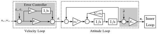
4.6. Linearized Error Controller

For the attitude loop, the second-order reference model is adopted and an additional proportional error controller can be added to enhance the tracking performance. For the relatively slowest velocity loop, integrators can be added to optimize control performance while enhancing robustness. Figure 6 demonstrates the structure of the error controller.

Figure 6. Error controller structure.

4.7. Protection Integration

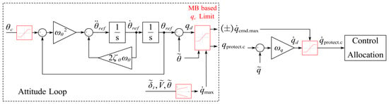
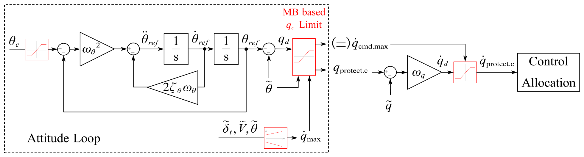
For the INDI controller, it is natural to integrate the saturation of $q_c$ into the attitude reference model and output ${\dot{q}}_{\lim }$ into the pseudo input for control allocation. The associated gain adjustment work for $K_{q.\mathrm{protect}}$ is almost negligible relative to traditional PID. The controller structure with pitch angle protection is demonstrated in Figure 7.

Figure 7. Protected pitch angle controller structure.

For cascaded PID controller, the same protection control method can be integrated. The control commands and control allocation scheme are similar to those of the INDI controller. The multi-loop control law can be written as:

$$\left\{\begin{array}{c}{a}_{Tc}=\left(K_{PV}{e}_V+K_{IV}\int e_V\mathrm{d}t\right)\cos \left(\theta +{\delta }_t\right)-\left(K_{P\dot{H}}{e}_{\dot{H}}+K_{I\dot{H}}\int e_{\dot{H}}\mathrm{d}t\right)\sin \left(\theta +{\delta }_t\right)\hfill \\ {\dot{p}}_d=K_{Pp}\left(K_{P\varphi }{e}_{\varphi }-\tilde{p}\right)\hfill \\ {\dot{q}}_d=K_{Pq}\left(K_{P\theta }{e}_{\theta }-q\right)+K_{Iq}\int \left(K_{P\theta }{e}_{\theta }-q\right)\mathrm{d}t\hfill \\ {\dot{r}}_d=K_{Pr}{e}_r\hfill \end{array}\right.$$

(54)

where feedback error terms are $e_V=u_{ec}-{\tilde{u}}_e,e_{\dot{H}}={\dot{H}}_c-\tilde{\dot{H}},e_{\varphi }={\varphi }_c-\tilde{\varphi },e_{\theta }={\theta }_c-\tilde{\theta },e_r=r_c-\tilde{r}$. The required ${\mathit{\nu }}_{\mathrm{Inner}}={\left[a_{Tc}{\dot{p}}_d{\dot{q}}_d{\dot{r}}_d\right]}^{\mathrm{T}}$ is then fed into control allocation.

The $q_{\lim }$ and ${\dot{q}}_{\lim }$ saturation are incorporated into ${\dot{\theta }}_{ref}=K_{P\theta }{e}_{\theta }$ and ${\dot{q}}_{ref}={\dot{q}}_d$, which are nominal $q_c$ and ${\dot{q}}_c$.

5. Simulation and Discussion

5.1. Transition Corridor and Protected Commands

The key parameters relevant to corridor prediction are provided by Table 2, which are determined based on publicly available data related to eVTOL aircraft [20,51].

Table 2. Key parameters [20,32,51].

Parameters	Value	Parameters	Value
m	$2000\mathrm{kg}$	$K_T$	1 Nm/A
$c_R$	1.5 m	$K_E$	1 V/(rad/s)
$S_R$	$14.9{\mathrm{m}}^2$	$N_{bs}$	200
$[{\beta }_1,{\beta }_2,{\beta }_3,{\beta }_4]$	[0.2076, 0.2288, 0.2037, 2.5529]	$N_{bp}$	30
$R_M$	$0.00985\mathsf{\Omega }$	$R_B$	$0.01\mathsf{\Omega }$
$D_p$	2.5 m	$N_p$	6

The transition corridor boundary should reflect the impact of electric-propulsive characteristics. Table 3 summarizes the constraints adopted in this study.

Table 3. Constraint parameters of the exemplary eVTOL [20,33,52,53].

Constraints	Lower Boundary	Upper Boundary
$\alpha$	$-{12}^{\circ }$	${12}^{\circ }$
${\delta }_e$	$-{25}^{\circ }$	${25}^{\circ }$
${\omega }_M$	$0\mathrm{RPM}$	$2000\mathrm{RPM}$
$P_M$	$0\mathrm{kW}$	$236\mathrm{kW}$
$Q_M$	$0\mathrm{Nm}$	$1380\mathrm{Nm}$
$I_B$	$0\mathrm{A}$	$2000\mathrm{A}$
$M_{tip}$	0	$0.85$

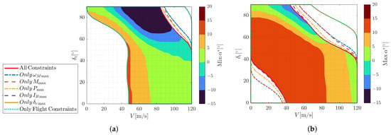
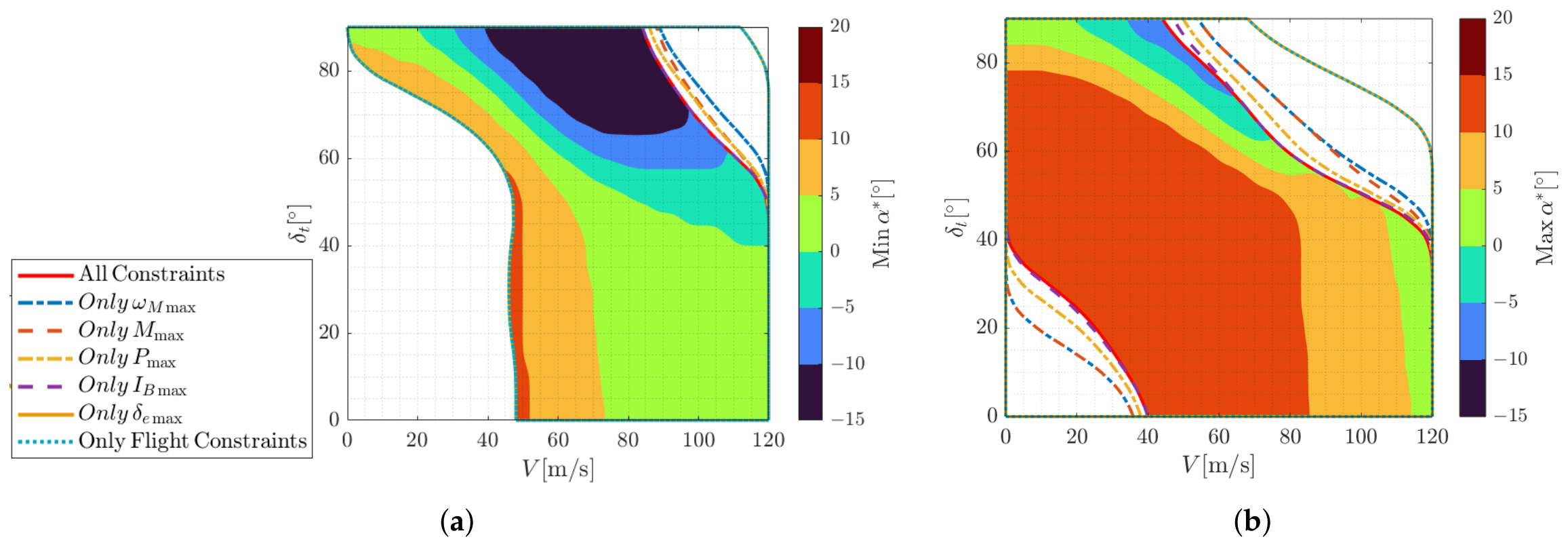
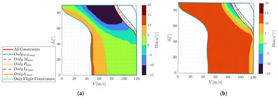
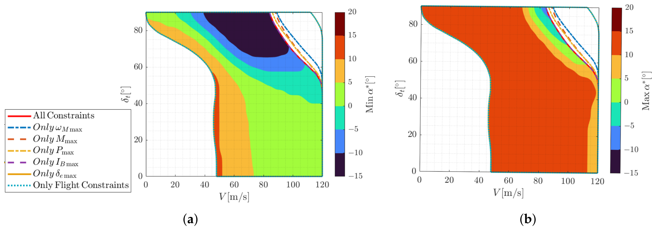
The corridor search resolutions are set to 1° for $\alpha$, 1 m/s for V and 1° for ${\delta }_t$. Figure 8 and Figure 9 respectively demonstrate the transition corridor and retransition corridor of the exemplary eVTOL, incorporating velocity and $\alpha$ boundaries. The trimmable $\alpha$ range is illustrated by the background color which enables intuitive observation of its variation with different tilt angles.

Figure 8. Transition boundary: (a) minimum attainable $\alpha$; (b) maximum attainable $\alpha$.

Figure 9. Retransition-capable boundary: (a) minimum attainable $\alpha$; (b) maximum attainable $\alpha$.

Figure 8 and Figure 9 compare the predicted corridor boundaries under individual constraints. The battery current limit dominates during transition, reducing $V_{\max }$ by 28 m/s on the basis of flight constraints and also affecting $V_{\min }$. The motor power limit has an intermediate influence, whereas motor speed limit ${\omega }_{M\max }$ and blade-tip limit $M_{\max }$ have minor effects. The elevator deflection limit has negligible influence due to differential thrust compensation. During retransition, electric constraints have weaker effects due to lower propulsion demands, with the battery current limit mainly restricting $V_{\max }$ at large tilt angles.

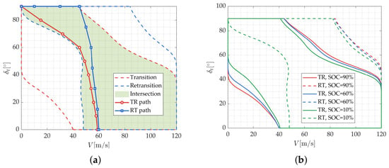
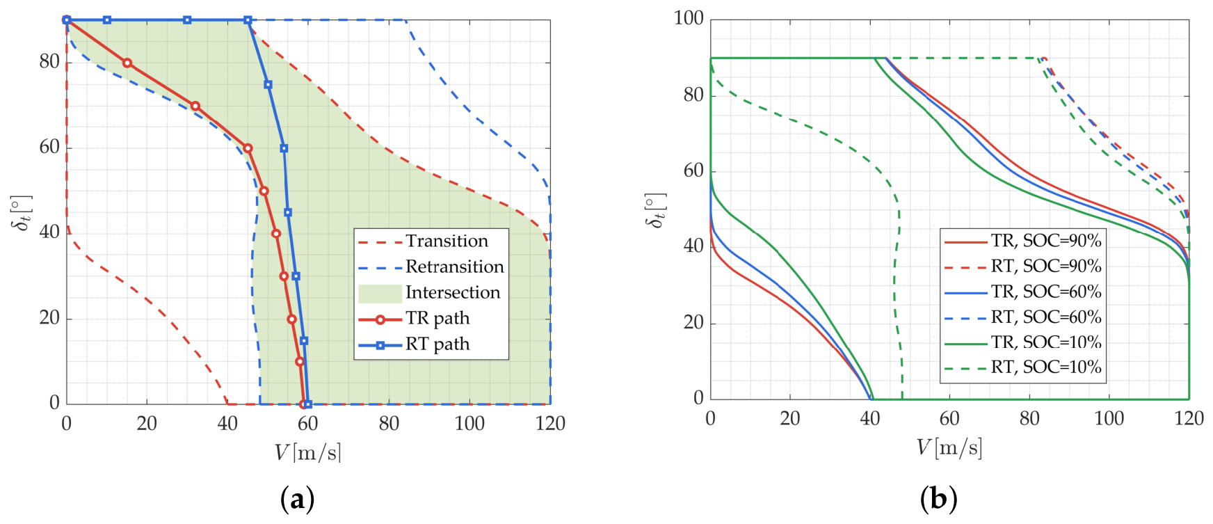
Figure 10a shows the intersection of transition and retransition corridors, which is a state region of both acceleration and deceleration capability. Transition paths are selected within the intersected corridor. Figure 10b shows the boundary variation of different SOC. Compared with the RT corridor, the feasible TR region contracts more significantly as SOC decreases. For retransition, SOC mainly affects the $V_{\max }$ boundary, which lies outside the intersected corridor.

Figure 10. Corridor boundary: (a) intersected boundary; (b) boundary variation under different SOC.

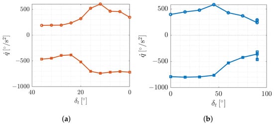
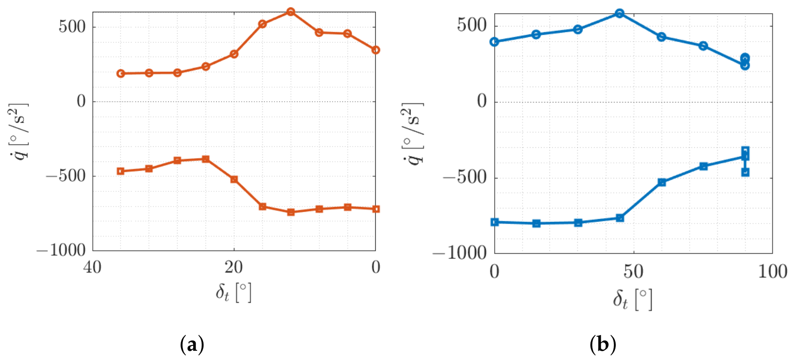
Each transition path corresponds to the attainable maneuverability $\dot{q}$, which is solved by the SQP solver with a constraint tolerance of ${10}^{-5}$, an optimality tolerance of ${10}^{-7}$, a step tolerance of ${10}^{-11}$ and a maximum of 800 iterations and 10,000 function evaluations. Figure 11a demonstrates the ${\dot{q}}_{\max \pm }$ associated with designated transition profile. ${\dot{q}}_{\max }$ generally increases in the later transition and peaks around middle transition, benefiting from rising dynamic pressure, which reduces the required powered lift and enhances aerodynamic control effectiveness. Figure 11b demonstrates the ${\dot{q}}_{\max \pm }$ associated with designated retransition profile, exhibiting a similar trend to that of the transition case.

Figure 11. Maneuverability boundary: (a) maneuverability boundary of transition; (b) maneuverability boundary of retransition.

Taking a linearized $q_{\lim }$ method as a baseline for comparison [23]:

$$\left\{\begin{array}{c}{q}_{\lim -}={\displaystyle \frac{{\theta }_{\lim -}-\theta }{\tau }}\hfill \\ q_{\lim +}={\displaystyle \frac{{\theta }_{\lim +}-\theta }{\tau }}\hfill \end{array}\right.$$

(55)

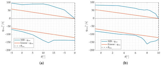
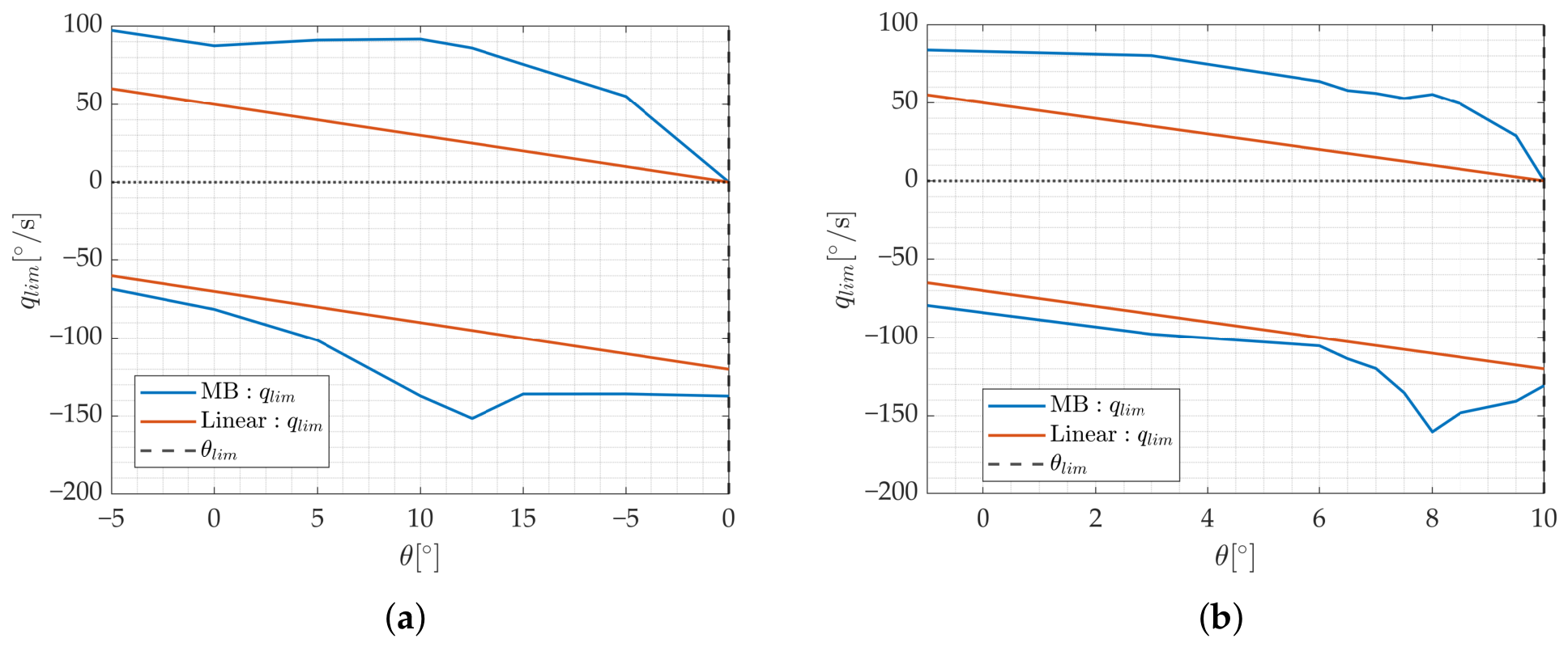
According to the definition in Section 3.1.3, pitch boundary ${\theta }_{\lim \pm }$ is mapped from the upper and lower boundary of $\alpha$ with $1^{\circ }$ safety margin. Thus, in this case, ${\theta }_{\lim \pm }$ is determined as $\pm {11}^{\circ }$. Figure 12 shows the comparison of linear $q_{\lim }$ and the MB $q_{\lim }$. The latter shows better adaptability to the instantaneous ${\dot{q}}_{\max }$.

Figure 12. Comparison of MB pitch rate limit and linear pitch rate limit ($\tau =0.5\mathrm{s}$): (a) protected $q_{\lim }$ corresponding to transition boundary; (b) protected $q_{\lim }$ corresponding to retransition boundary.

5.2. Profile Assessment for Protected Controller

This paper is not intended for comprehensive assessment. Instead, the primary objective is to evaluate the nominal performance and robustness of the protected control mechanism by specific mission tasks [54].

5.2.1. Nominal Profile Simulation

The mission profile should reflect the following elements [55]:

• The adaptability of eVTOL operation in a low-altitude environment.
• The attitude and altitude stability with sufficient and smooth actuator usage.

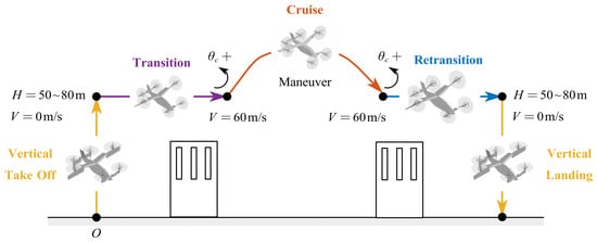
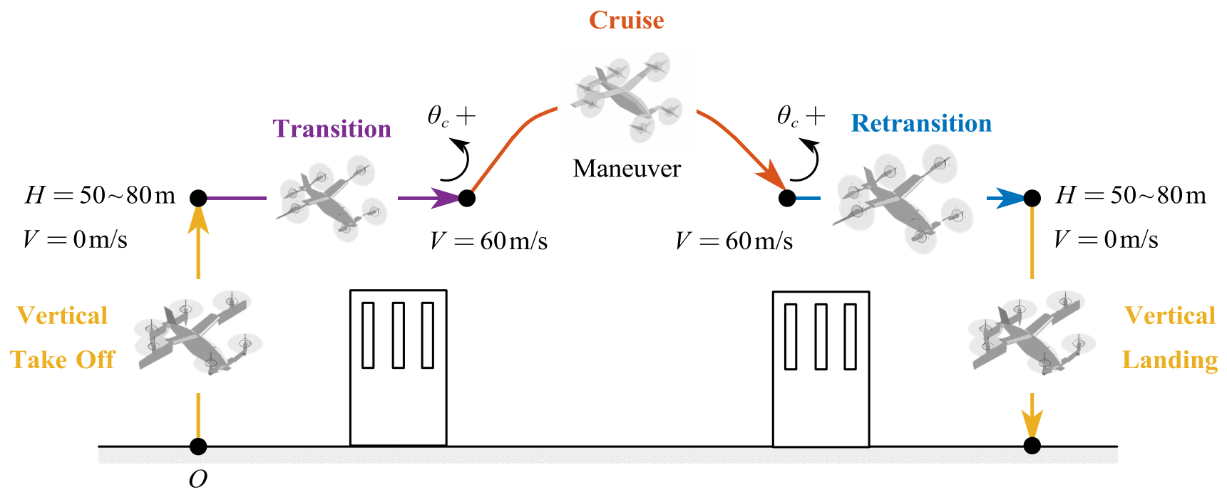
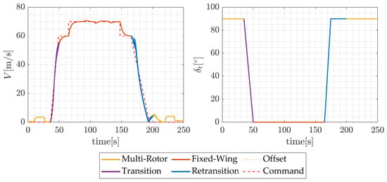
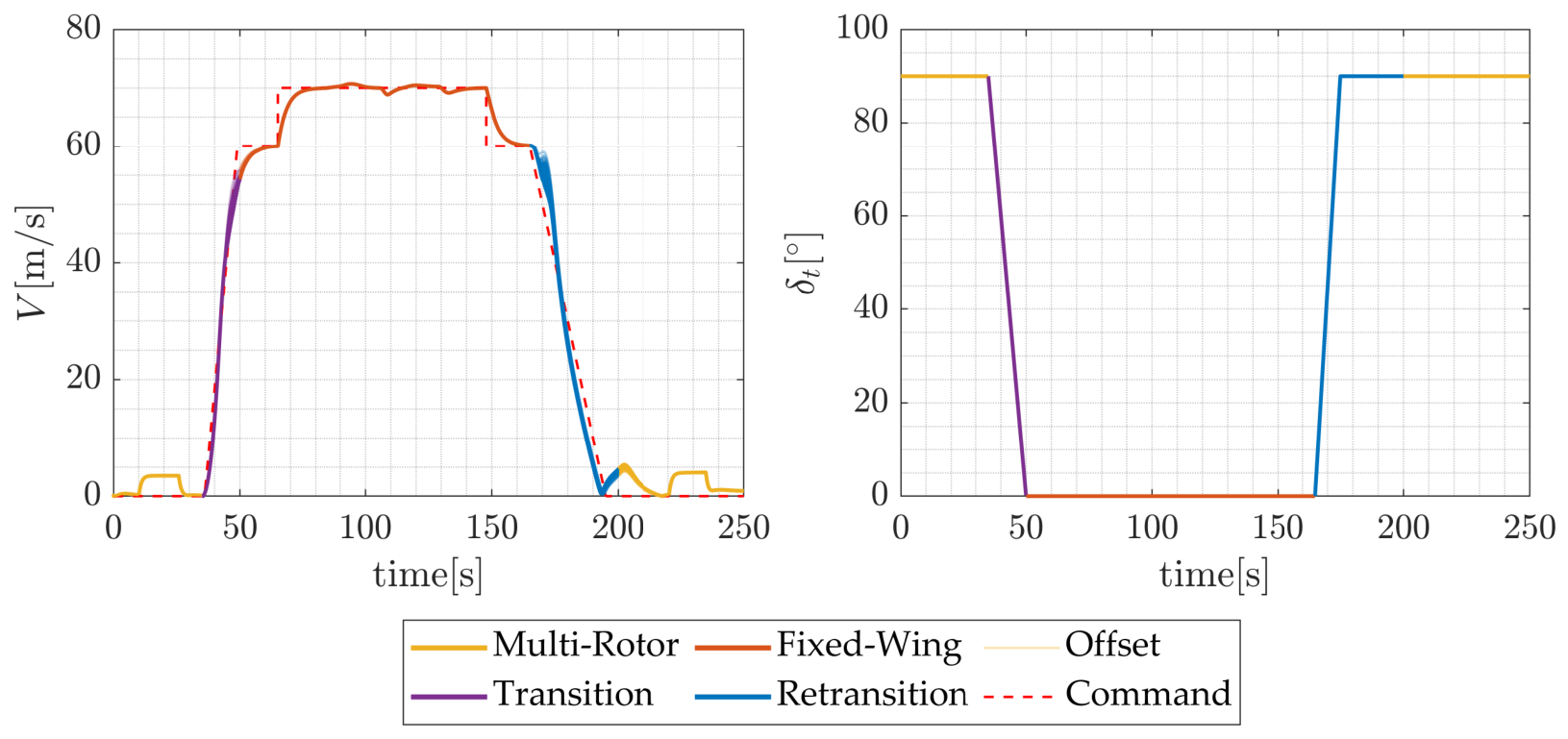
Based on this consideration, a mission profile is designed as shown in Figure 13. First, take off vertically to the height of 50–80 m, which is an altitude above most of the buildings around airport. Then, start transition and tilt from ${90}^{\circ }$ to $0^{\circ }$ to accelerate from hovering to cruising velocity of 60 m/s. During cruising, the middle and rear propellers are deactivated. Accelerate to 70 m/s and execute a roll maneuver to examine roll control channels. Finally, decelerate to 60 m/s and enter retransition to continue deceleration to hovering, with tilt angle increasing to ${90}^{\circ }$. Height of 50–80 m is still required to avoid obstacles. Finally, the aircraft descends vertically to the landing site. Excessive nose-up commands are incorporated into the final transition and initial retransition, where nose-up maneuvers are required to establish aerodynamic lift and decelerate the aircraft, respectively.

Figure 13. Full mission profile for simulation.

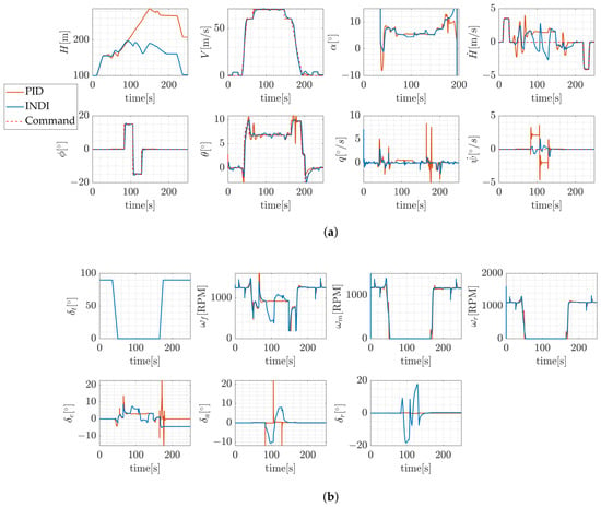
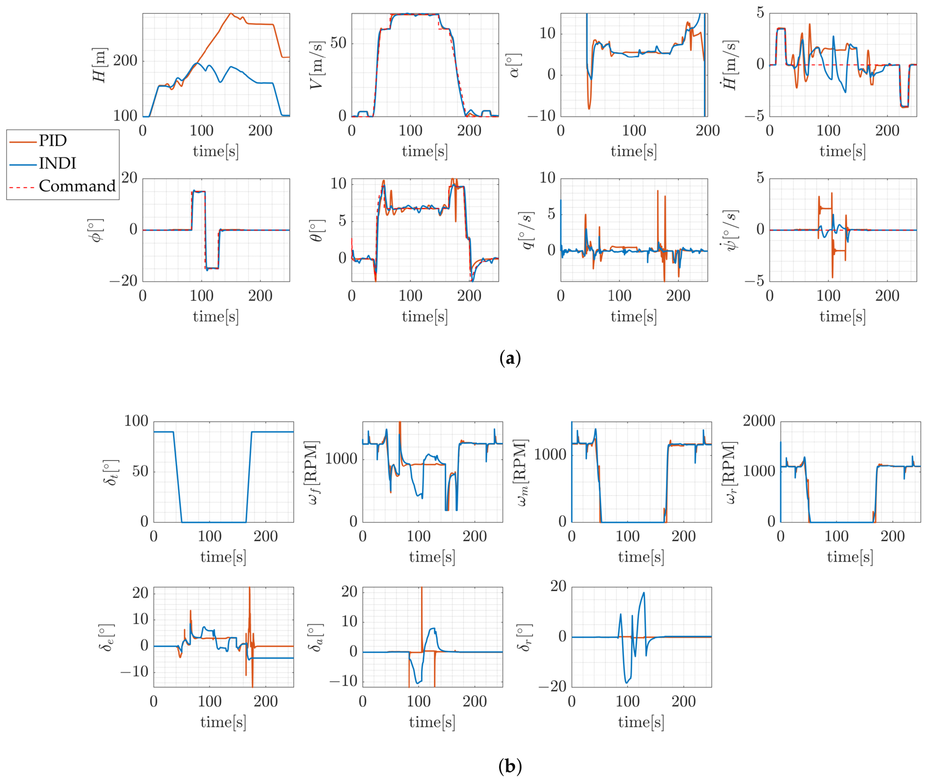
First, Figure 14a,b show the response comparison. Under nominal pitch command, both controllers successfully complete the transition mission, indicating satisfactory nominal control performance within actuator boundaries.

Figure 14. Nominal simulation results: (a) responses of INDI and PID controllers; (b) required actuations of INDI and PID controllers.

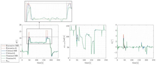
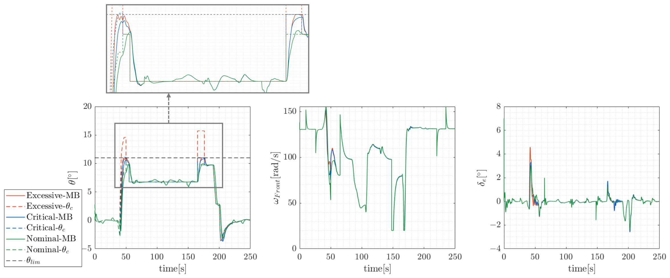
Second, Figure 15 illustrates the responses of protected INDI controller to pitch commands of excessive, critical and nominal amplitudes. The nominal control performance is well preserved and the protection strategy is effective under excessive command.

Figure 15. Response of protected INDI controller of different pitch commands (with an enlarged view of the protection-activated region).

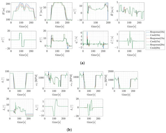
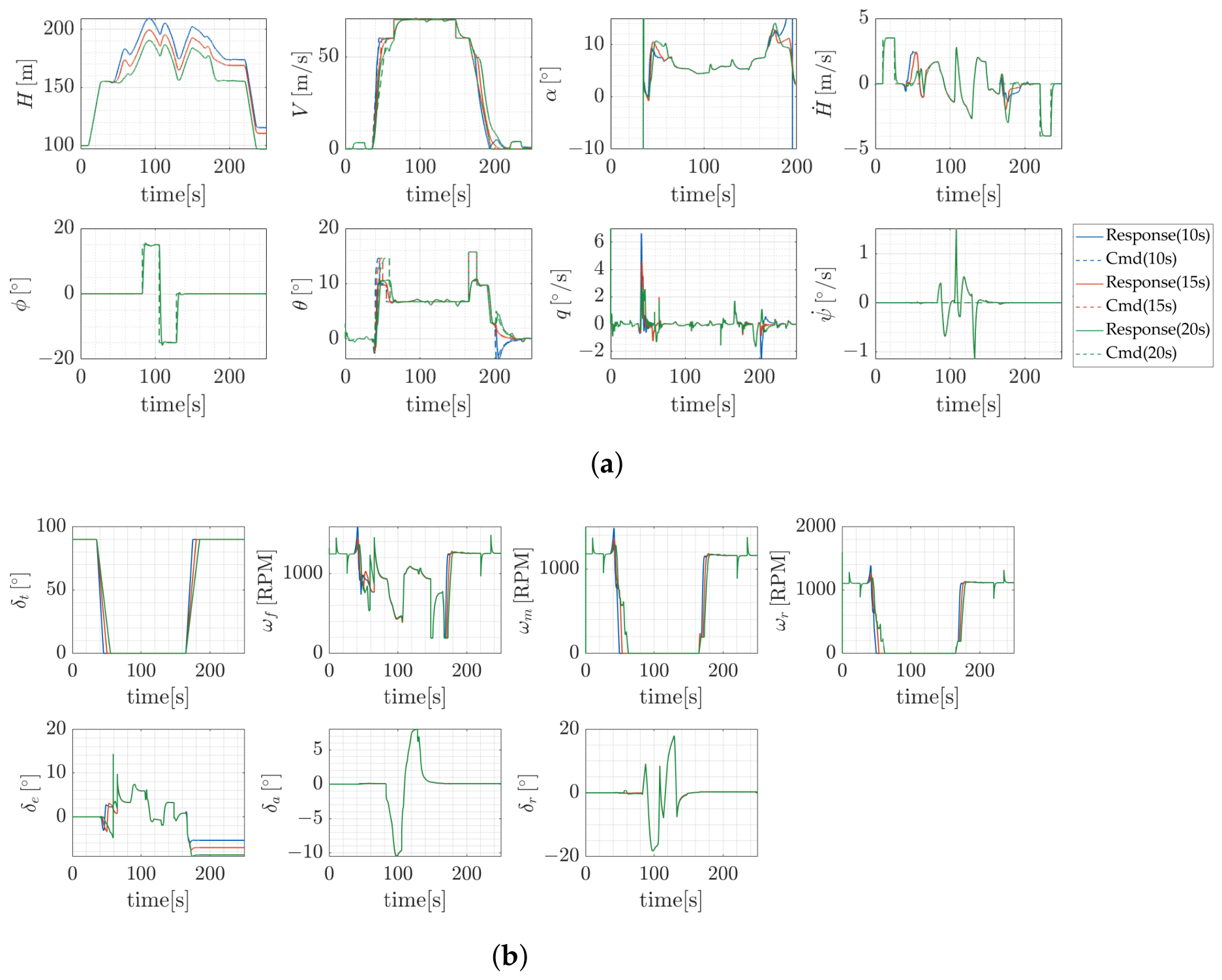
Third, Figure 16a,b illustrate the responses of protected INDI controller under nominal, faster and slower tilt-velocity scheduling profiles under the same excessive pitch command. The results indicate satisfactory tracking performance, supporting the applicability of the proposed method under the prescribed transition conditions.

Figure 16. Simulation results of various tilt-velocity: (a) responses of different tilt-velocity profiles; (b) required actuations of different tilt-velocity profiles.

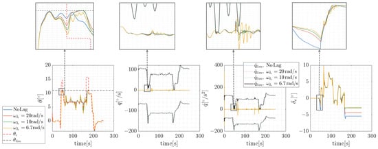
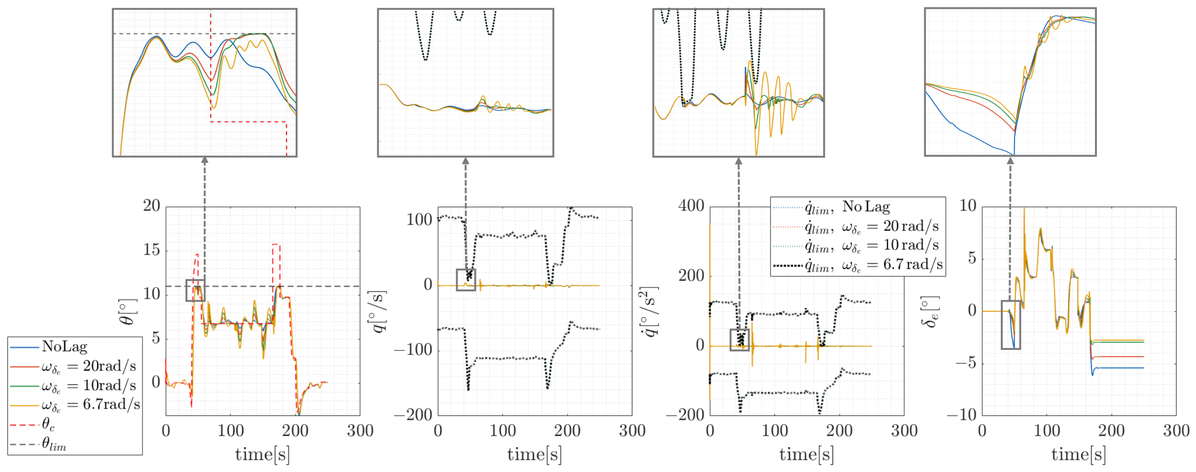
Moreover, Figure 17 demonstrates the simulations with different elevator actuator bandwidths under the same pitch commands. The elevator actuator dynamics are modeled as a first-order element. The bandwidths are selected to represent relatively fast, nominal and slow actuator responses [56].

Figure 17. Response of protected INDI controller of different bandwidths.

As the bandwidth decreases, the INDI controller exhibits degraded tracking performance due to the absence of actuator dynamics compensation. Noticeable oscillations appear at ${\omega }_{{\delta }_e}=6.7\mathrm{rad}/\mathrm{s}$. Nevertheless, the results indicate that the proposed protection strategy remains effective within the investigated bandwidth range although actuator lag affects closed-loop response characteristics.

5.2.2. Perturbed Profile Simulation

Since eVTOLs feature complex nonlinear dynamics, linear methods are unable to cover the full-envelope control stability and robustness assessment. A stochastic method such as Monte Carlo (MC) is employed to evaluate nonlinear controller performance under practical uncertainties [57]. The protected PID controller serves as a benchmark for evaluating the robustness of the protected INDI controller [50].

Among the uncertainty factors, aerodynamic model and measurement uncertainties are considered in the present study because they have pronounced effects on the proposed protection framework. First, aerodynamic model uncertainty parameters are selected according to the blending model rather than varying individual aerodynamic coefficients. A combined deviation of the mid-point $\overline{{\delta }_t}$ and slope parameters k is performed. Their uncertainties are suitable to be characterized by relative errors, thus multiplicative perturbation is adopted with a normal distribution [58].

For measurement uncertainties, deviation on pitch angle signal is mainly considered because it directly influences the protection effect. Even when angular rate measurements are pre-calibrated, attitude errors may still arise from gyro bias and accelerometer errors [59]. The perturbed pitch angle signal is represented by:

$$\tilde{\theta }=b_{\theta }+k_{\theta }\theta$$

(56)

where $k_{\theta }$ denotes the scale factor error and $b_{\theta }$ denotes the additive bias. Uncertainties arising from scale-factor such as manufacturing and temperature variations are suitable to be characterized by relative errors. Uncertainties arising from bias such as gyro bias, installation misalignment and calibration are suitable to be characterized by absolute errors. Table 4 presents the selection of distribution parameters and their references.

Table 4. Uncertainty parameters.

Uncertainty	Distribution	Parameters	Parameter Reference
k	Normal; Multiplicative	$3\sigma =0.5,\mu =1$	Reported aerodynamic uncertainty spread settings [57]
$\overline{{\delta }_t}$	Normal; Multiplicative	$3\sigma =0.5,\mu =1$
$k_{\theta }$	Normal; Multiplicative	$\sigma =0.005,\mu =1$	Reported gyro scale factor error range [60]
$b_{\theta }$	Uniform; Additive	$\left[-1^{\circ },1^{\circ }\right]$	Commercial AHRS accuracy [43]

Following ref. [61], given a target violation probability of $\epsilon =0.01$, $N=500$ MC simulations provide a detection confidence level as $1-\delta =1-{(1-\epsilon )}^N=99.34\%$. Therefore, the number of MC samples is selected as 500. The simulation task follows the profile in Figure 13 with excessive nose-up commands injected in transition and retransition. For brevity, the tilt angle and forward velocity responses are first presented together in Figure 18, while the subsequent figures focus on pitch protection performance under different uncertainty conditions. Lines in different colors represent different flight phases.

Figure 18. Responses of tilt angle and forward velocity in perturbed simulation.

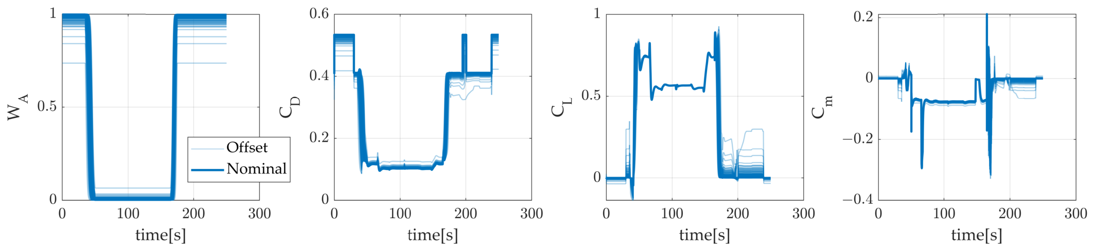
For aerodynamic uncertainties assessment, Figure 19 shows the perturbed $W_A$ and aerodynamic coefficients.

Figure 19. $W_A$ Deviation and corresponding $C_L,C_D,C_m$.

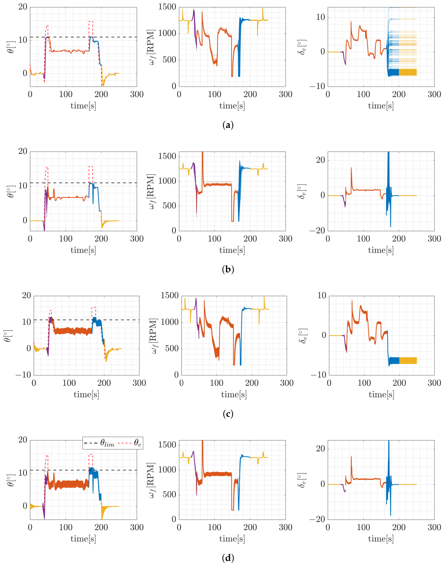
Figure 20a,b demonstrate that both protected INDI and protected PID with excessive pitch commands exhibit satisfactory pitch protection performance under aerodynamic model uncertainties, indicating that the proposed protection strategy is compatible with both conventional feedback control and nonlinear model-based control architectures. Figure 20c,d demonstrate that pitch measurement uncertainties introduce more noticeable variations in pitch responses. The reason is that the protection mechanism relies on pitch angle signal accuracy, thus measurement uncertainties inevitably introduce the possibility of constraint violation. This highlights the importance of reserving safety margin to reduce the risk of boundary violation.

Figure 20. Perturbed simulation results: (a) protected INDI under $W_A$ uncertainties; (b) protected PID under $W_A$ uncertainties; (c) protected INDI under $\theta$ measurement uncertainties; (d) protected PID under $\theta$ measurement uncertainties.

Further, introduce the following statistical indicators to indicate violation level and tracking performance under uncertainties:

(a)

Mean absolute error ($MAE$): the absolute tracking error averaged by time [62].

(b)

Maximum pitch-angle boundary violation ($\mathsf{\Delta }{\theta }_{\max }$): the maximum exceedance of pitch angle beyond the prescribed pitch-angle protection boundary over the profile [63].

(c)

Violation probability ($P_{\mathrm{vio}}$): the proportion of MC runs in which pitch angle exceeds the prescribed pitch-angle protection boundary at least once over the profile [63].

$MAE$ serves as the tracking performance indicator, while $\mathsf{\Delta }{\theta }_{\max }$ and $P_{\mathrm{vio}}$ serve as the safety indicators. Their mean value $\mu$ and standard deviation $\sigma$ are calculated across MC runs. Table 5 illustrates the comparison of the statistical indicators of the perturbed simulation.

Table 5. Deviation statistical results.

Uncertainty	Controller	Statistical Indicators
		${\mathit{\mu }}_{\mathit{MAE}}$	${\mathit{\sigma }}_{\mathit{MAE}}$	${\mathit{\mu }}_{\mathbf{\Delta }{\mathit{\theta }}_{\mathbf{max}}}$	${\mathit{\sigma }}_{\mathbf{\Delta }{\mathit{\theta }}_{\mathbf{max}}}$	${\mathit{P}}_{\mathbf{vio}}$
$W_A$	PID	${0.71}^{\circ }$	${0.0058}^{\circ }$	$0^{\circ }$	$0^{\circ }$	$0\%$
(Aerodynamics)	INDI	${0.76}^{\circ }$	${0.0029}^{\circ }$	$0^{\circ }$	$0^{\circ }$	$0\%$
$\tilde{\theta }$	PID	${0.93}^{\circ }$	${0.14}^{\circ }$	${0.19}^{\circ }$	${0.07}^{\circ }$	44.8%
(Measurement)	INDI	${1.04}^{\circ }$	${0.21}^{\circ }$	${0.25}^{\circ }$	${0.10}^{\circ }$	50.4%

The quantitative comparison shows that protected PID and INDI exhibit comparable tracking performance, with no boundary violations under aerodynamic model uncertainties. Although pitch measurement uncertainties cause more noticeable tracking deviations and violations of the prescribed pitch-angle protection boundaries, the mean maximum violations remain below the prescribed 1° safety margin. Compared with PID, INDI exhibits smaller response dispersion under aerodynamic uncertainties but greater dispersion under pitch measurement uncertainties, suggesting that the protected-INDI controller established in this study is more sensitive to measurement accuracy.

5.3. Comparison of Different Protection Strategy

The simulation task follows the profile in Figure 13, under the same excessive pitch command injected.

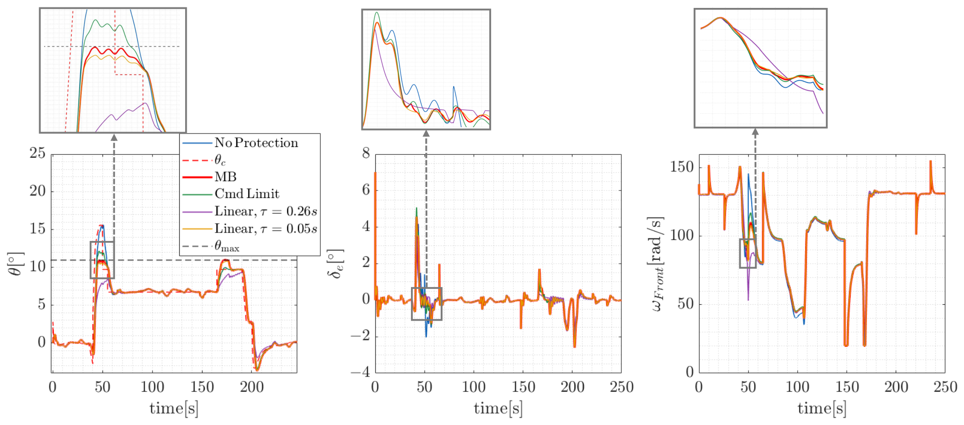
For the linear protection method, the protection time constant $\tau$ represents the predicted time to reach the pitch boundary at the current pitch rate [23]. Its reference value is first estimated based on its physical interpretation. From the unprotected pitch response during transition, $\theta$ first approaches the upper pitch boundary with $1^{\circ }$ margin at $q={3.94}^{\circ }/\mathrm{s}$, indicating a reference $\tau ={\displaystyle \frac{{\theta }_{\lim +}-\theta \left(t_a\right)}{q\left(t_a\right)}}={\displaystyle \frac{{11}^{\circ }-{9.96}^{\circ }}{{3.94}^{\circ }/\mathrm{s}}}=0.26\mathrm{s}$. A smaller $\tau$ is also considered to show the influence of parameter tuning on protection performance.

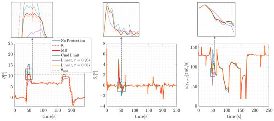
Figure 21 demonstrates the performance of the INDI controller with different protection strategies. The blue line corresponds to the response without protection, which is apparently worse than the others. The red line corresponds to the MB dynamic protection proposed by this paper, staying between the green line, which is the response with only ${\theta }_c$ limit, and the purple and yellow lines, which are responses with linear protection with different time constants. It can be seen that the MB method can effectively constrain the state with smooth control resources consumption.

Figure 21. Comparison of pitch protection strategies on INDI controller.

In addition to $MAE$ and $\mathsf{\Delta }{\theta }_{\max }$, the total variation of control inputs ($TV$), defined as the cumulative variation in control inputs, is introduced as an indicator of control input smoothness [64]. Table 6 illustrates the quantitative comparison of different protection strategies. It shows that the MB method effectively eliminates pitch boundary violations while maintaining moderate tracking errors and control input variations. Compared with the unprotected case, the MB method reduces control input variations, whereas command limiting alone still results in a maximum boundary violation of 1.19°. For linear protection, different $\tau$ selection greatly affects the protection effect. The $\tau =0.05\mathrm{s}$ case indicates that certain parameter settings at this specific condition can achieve protection performance comparable to that of the proposed method. However, identical response characteristics do not necessarily extend to other operating conditions.

Table 6. Quantitative comparison of different protection strategies.

Protection Strategy	Performance Indicators
	MAE	$\mathsf{\Delta }{\mathit{\theta }}_{\max }$	${\mathit{TV}}_{{\mathit{\delta }}_{\mathit{e}}}$	${\mathit{TV}}_{{\mathit{\omega }}_{\mathit{f}}}$
No Protection	${0.54}^{\circ }$	${4.66}^{\circ }$	${81.7}^{\circ }$	$1071.8\mathrm{RPM}$
MB Protection	${0.77}^{\circ }$	$0^{\circ }$	${68.5}^{\circ }$	$992.1\mathrm{RPM}$
Command Limit	${0.56}^{\circ }$	${1.19}^{\circ }$	${69.2}^{\circ }$	$992.6\mathrm{RPM}$
Linear Protection ($\tau =0.26\mathrm{s}$)	${0.95}^{\circ }$	$0^{\circ }$	${62.7}^{\circ }$	$1004\mathrm{RPM}$
Linear Protection ($\tau =0.05\mathrm{s}$)	${0.78}^{\circ }$	$0^{\circ }$	${67.1}^{\circ }$	$989.4\mathrm{RPM}$

6. Conclusions

This study developed a corridor-based protected control framework for tilt-wing eVTOL, including constrained corridor prediction, maneuverability-based pitch protection strategy and its integration with nonlinear model-based controller. The main contributions and findings of this study are summarized as follows:

(a)

A 6-DOF flight dynamic model of a 3-surface tilt-wing eVTOL was established, incorporating component-level electric propulsion dynamics. The model provides the foundation for validating transition corridor prediction, envelope protection and the unified control algorithm.

(b)

A corridor prediction method was proposed by incorporating aerodynamic, electrical and propulsive constraint models. Both acceleration and deceleration feasibility were evaluated to identify admissible regions of transition states. The results reveal that the predicted corridor reflects the multi-physics constraints and provides the basis for deriving pitch protection boundaries.

(c)

A maneuverability-based protected control strategy was proposed to automatically generate pitch rate and pitch angular acceleration limits according to the current control margin instead of relying on simple linear pitch rate limitation. Nominal and perturbed profile simulations demonstrated generally effective pitch protection under the investigated conditions, despite degraded tracking performance with increasing actuator lag and limited boundary violations under pitch measurement uncertainties.

(d)

The profile simulation results demonstrate that the proposed protection strategy is compatible with both conventional feedback control and model-based nonlinear control. Its integration with INDI exhibits potential to facilitate controller tuning.

Generally speaking, the results indicate that the proposed protected control framework provides effective corridor-based protection while maintaining maneuverability under the investigated nominal and perturbed transition conditions. The study therefore establishes a practical link between transition corridor prediction, available maneuvering capability and closed-loop control protection for tilt-wing eVTOL transition flight.

Current work primarily focuses on pitch protection, with protection boundaries derived under the nominal level-flight assumption. The nominal simulations consider different controller architectures and specific pitch command amplitudes, tilt profiles and actuator time constants, while the robustness evaluation covers selected aerodynamic model and pitch measurement uncertainties. Future work can extend the framework to non-level transition conditions, dynamically reachable flight boundaries, broader uncertainties/disturbances/failures and generalize the protection framework to lateral-directional constraints. Furthermore, hardware-in-the-loop simulations and flight tests will be conducted to validate the practical applicability of the proposed strategy.

References

- Airbus. Vahana|Airbus. Available online: https://www.airbus.com/en/innovation/low-carbon-aviation/urban-air-mobility/cityairbus-nextgen/vahana (accessed on 16 March 2026).
- Joby, A. Joby Completes Piloted Electric Air Taxi Flight Across San Francisco Bay and Around the Golden Gate. Available online: https://ir.jobyaviation.com/news-events/press-releases/detail/177/joby-completes-piloted-electric-air-taxi-flight-across-sane (accessed on 13 March 2026).
- Du, S.; Zha, Y. Numerical simulation of the transition flight aerodynamics of cross-shaped quad-tiltrotor UAV. Sci. Rep. 2024, 14, 17878. [Google Scholar] [CrossRef] [Scilit] [PubMed]
- Erhard, R.M.; Alonso, J.J. A Comparison of Propeller Wake Models for Distributed Electric Propulsion and eVTOL Aircraft in Complex Flow Conditions. In Proceedings of the AIAA SCITECH 2022 Forum, San Diego, CA, USA & Virtual, 3–7 January 2022. [Google Scholar] [CrossRef] [Scilit]
- Ducard, G.J.; Allenspach, M. Review of designs and flight control techniques of hybrid and convertible VTOL UAVs. Aerosp. Sci. Technol. 2021, 118, 107035. [Google Scholar] [CrossRef] [Scilit]
- Hsu, T.W.; Choi, J.J.; Amin, D.; Tomlin, C.; McWherter, S.C.; Piedmonte, M. Towards Flight Envelope Protection for the NASA Tiltwing eVTOL Flight Mode Transition Using Hamilton-Jacobi Reachability. J. Am. Helicopter Soc. 2024, 69, 1–18. [Google Scholar] [CrossRef] [Scilit]
- Liang, Z.; Yang, X.; Liu, D.; Hou, Z.; Fan, L. Multi-objective constrained tilt corridor and transition trajectory strategy of a compound tilt-rotor UAV. Chin. J. Aeronaut. 2025, 39, 103898. [Google Scholar] [CrossRef] [Scilit]
- May, M.S.; Milz, D.; Armanini, S.F. Transition Corridor Estimation for a Tilt-Wing Aircraft with Optimal Control-based Reachability Analysis. In Proceedings of the AIAA SCITECH 2026 Forum, Orlando, FL, USA, 12–16 January 2026. [Google Scholar] [CrossRef] [Scilit]
- Yue, H.; Gao, Z.; Liu, P.; Wang, Z.; Li, J.; Shao, X.; Li, S.; Zhao, W. Transition planning and control methods for a tilt-wing VTOL UAV: From hardware design to flight validation. Aerosp. Sci. Technol. 2026, 168, 111265. [Google Scholar] [CrossRef] [Scilit]
- Kang, N.; Lu, L.; Whidborne, J. Energy Optimization Strategies for Automatic Tiltrotor eVTOL Aircraft. J. Guid. Control Dyn. 2025, 48, 1196–1200. [Google Scholar] [CrossRef] [Scilit]
- May, M.S.; Milz, D.; Looye, G. Transition Strategies for Tilt-Wing Aircraft. In Proceedings of the AIAA SCITECH 2024 Forum, Orlando, FL, USA, 8–12 January 2024. [Google Scholar] [CrossRef] [Scilit]
- EPIC. Managing Range and Endurance of Battery-Electric Aircraft; GAMA: Washington, DC, USA, 2023. [Google Scholar]
- Ogden, N.C.; Patterson, A. A Framework for Evaluating Distributed Electric Propulsion on the SUSAN Electrofan Aircraft; Number NASA/TM–20230009523; NASA: Washington, DC, USA, 2023. [Google Scholar]
- Lu, Z.; Zhang, J.; Li, H.; Holzapfel, F. An Adaptive Command Scaling Method for Incremental Flight Control Allocation. Actuators 2025, 14, 579. [Google Scholar] [CrossRef] [Scilit]
- Han, L.; Zhang, P.; Wang, Y.; Bian, Y.; Hu, J. A Computational Method for the Nonlinear Attainable Moment Set of Tailless UAVs in Flight-Control-Oriented Scenarios. Drones 2025, 9, 585. [Google Scholar] [CrossRef] [Scilit]
- May, M.S.; Milz, D.; Looye, G. Towards the Determination of the Dynamic Transition Corridor for Tandem Tilt-Wing Aircraft. In Proceedings of the AIAA Aviation Forum and Ascend 2024, Las Vegas, NV, USA, 29 July–2 August 2024. [Google Scholar] [CrossRef] [Scilit]
- Chauhan, S.S.; Martins, J.R.R.A. Tilt-Wing eVTOL Takeoff Trajectory Optimization. J. Aircr. 2020, 57, 93–112. [Google Scholar] [CrossRef] [Scilit]
- Kikumoto, C.; Urakubo, T.; Sabe, K.; Hazama, Y. Analysis and Enhancement of Steady Climb Performance with Control Input Redundancy for a Dual-Propulsion VTOL UAV. Aerospace 2026, 13, 316. [Google Scholar] [CrossRef] [Scilit]
- Li, W.; Cheng, R.; Huang, H.; Garg, A.; Gao, L. Energy consumption modeling and optimization of an eVTOL aircraft: Integrating weight, motor, and battery dynamics. Energy 2025, 325, 136229. [Google Scholar] [CrossRef] [Scilit]
- Wang, M.; Li, X.; Zhang, S. A Cascaded trim method of electric aircraft subject to propulsive constraints in wing-borne flight. Aerosp. Sci. Technol. 2026, 171, 111589. [Google Scholar] [CrossRef] [Scilit]
- May, M.; Milz, D.; Armanini, S.F. An Optimal Control Approach for Harmonizing Tilt-Wing Design and Operations. In Aerospace Systems; Springer: Berlin/Heidelberg, Germany, 2026. [Google Scholar] [CrossRef] [Scilit]
- Lombaerts, T.; Looye, G.; Ellerbroek, J.; Rodriguez, Y.; Martin, M. Design and Piloted Simulator Evaluation of Adaptive Safe Flight Envelope Protection Algorithm. In Proceedings of the AIAA Guidance, Navigation, and Control Conference, San Diego, CA, USA, 4–8 January 2016. [Google Scholar] [CrossRef] [Scilit][Green Version]
- Gabrys, A.C.; Steffensen, R.; Cordeiro, R.D.A.; Azinheira, J.R.; Moutinho, A.; Holzapfel, F. Integration of Phase Plane Flight Envelope Protections in Cascaded Incremental Flight Control. IFAC-PapersOnLine 2019, 52, 429–435. [Google Scholar] [CrossRef] [Scilit]
- Bhardwaj, P.; Holzapfel, F. Unified Trajectory Control for Vertical Take-Off and Landing Transition Aircraft. In Proceedings of the AIAA Aviation Forum and Ascend 2024, Las Vegas, NV, USA, 29 July–2 August 2024. [Google Scholar] [CrossRef] [Scilit]
- Milz, D.; May, M.S.; Armanini, S.F.; Looye, G. Stability and Robustness of a Tandem Tilt-Wing VTOL with Dynamic Inversion Control Laws. In Proceedings of the AIAA SCITECH 2026 Forum, Orlando, FL, USA, 12–16 January 2026. [Google Scholar] [CrossRef] [Scilit]
- Binz, F.; Islam, T.; Moormann, D. Attitude control of tiltwing aircraft using a wing-fixed coordinate system and incremental nonlinear dynamic inversion. Int. J. Micro Air Veh. 2019, 11, 1756829319861370. [Google Scholar] [CrossRef] [Scilit]
- Stougie, J.; Pollack, T.; Van Kampen, E.J. Incremental Nonlinear Dynamic Inversion control with Flight Envelope Protection for the Flying-V. In Proceedings of the AIAA Scitech 2024 Forum, Orlando, FL, USA, 8–12 January 2024. [Google Scholar] [CrossRef] [Scilit]
- Altunkaya, E.Ç.; Çatak, A.; Koyuncu, E.; Özkol, İ. Loss-of-Control Prevention of an Agile Aircraft: Dynamic Command Saturation Approach. J. Guid. Control Dyn. 2025, 48, 424–436. [Google Scholar] [CrossRef] [Scilit]
- Lu, Z.; Zhang, J.; Li, H.; Holzapfel, F. A virtual command protection strategy for pseudo-inverse flight control allocation. Aerosp. Sci. Technol. 2026, 168, 111134. [Google Scholar] [CrossRef] [Scilit]
- Sun, D.; Li, X.; Jafarnejadsani, H.; Hovakimyan, N. A Flight Envelope Protection Method Based on Potential Functions. In Proceedings of the AIAA Guidance, Navigation, and Control Conference, Grapevine, TX, USA, 9–13 January 2017. [Google Scholar] [CrossRef] [Scilit]
- Budihartono, M.; Martinez, E.; Moncayo, H.; Bustamante, F.; Clardy, J. Flight-Envelope Informed Control Barrier Function Constraints for Safety-Critical Pilot-in-the-Loop NASA GUAM VTOL. In Proceedings of the AIAA Aviation 2026 Forum, San Diego, CA, USA, 8–12 June 2026. [Google Scholar] [CrossRef] [Scilit]
- National Campaign Joby Activity Team. UAM Instrument Flight Procedure Design and Evaluation in the Joby Flight Simulator; Technical Report AAM-NC-115-001; NASA: Washington, DC, USA, 2023. [Google Scholar]
- Huang, Q.; He, G.; Jia, J.; Hong, Z.; Yu, F. Numerical Simulation on Aerodynamic Characteristics of Transition Section of Tilt-Wing Aircraft. Aerospace 2024, 11, 283. [Google Scholar] [CrossRef] [Scilit]
- Enenakpogbe, E.; Whidborne, J.F.; Lu, L. Full Envelope Control of Over-Actuated Fixed-Wing Vectored Thrust eVTOL. Aerospace 2024, 11, 979. [Google Scholar] [CrossRef] [Scilit]
- Irmawan, E.; Harjoko, A.; Dharmawan, A. Model, Control, and Realistic Visual 3D Simulation of VTOL Fixed-Wing Transition Flight Considering Ground Effect. Drones 2023, 7, 330. [Google Scholar] [CrossRef] [Scilit]
- Wang, M.; Diepolder, J.; Zhang, S.; Söpper, M.; Holzapfel, F. Trajectory optimization-based maneuverability assessment of eVTOL aircraft. Aerosp. Sci. Technol. 2021, 117, 106903. [Google Scholar] [CrossRef] [Scilit]
- Wang, M.; Luiz, S.O.D.; Zhang, S.; Lima, A.M.N. Desensitized Optimal Control of Electric Aircraft Subject to Electrical–Thermal Constraints. IEEE Trans. Transp. Electrif. 2022, 8, 4190–4204. [Google Scholar] [CrossRef] [Scilit]
- Panish, L.; Bacic, M. Tiltwing eVTOL Transition Trajectory Optimization. J. Aircr. 2025, 62, 81–93. [Google Scholar] [CrossRef] [Scilit]
- Jamaluddin, N.S.; Celik, A.; Baskaran, K.; Rezgui, D.; Azarpeyvand, M. Aerodynamic noise analysis of tilting rotor in edgewise flow conditions. J. Sound Vib. 2024, 582, 118423. [Google Scholar] [CrossRef] [Scilit]
- Sanchez-Carmona, A.; Sznajdrowicz-Rebisz, K.; Dominguez-Tuya, A.; Balsalobre-Alvarez, C.; Gandia-Aguera, F.; Cuerno-Rejado, C. Multi-Point Design of Optimal Propellers for Remotely Piloted Aircraft Systems. Aerospace 2025, 12, 860. [Google Scholar] [CrossRef] [Scilit]
- Johansen, T.A.; Fossen, T.I. Control allocation—A survey. Automatica 2013, 49, 1087–1103. [Google Scholar] [CrossRef] [Scilit]
- Deng, J.; Yang, Y.; Zhu, J.; Liao, W.; Yuan, X.; Wang, X. Pigeon-Inspired Transition Trajectory Optimization for Tilt-Rotor UAVs. Drones 2025, 9, 432. [Google Scholar] [CrossRef] [Scilit]
- VectorNav Technology. VectorNav’s VN-100 IMU/AHRS, the World’s Most Trusted Surface Mount Solution. Available online: https://www.vectornav.com/products/detail/vn-100 (accessed on 28 September 2026).
- Milz, D.; May, M.; Looye, G. Tandem Tilt-Wing Control Law Design Using Hybrid Nonlinear Dynamic Inversion. J. Guid. Control Dyn. 2026, 49, 1566–1574. [Google Scholar] [CrossRef] [Scilit]
- Milz, D.; Looye, G. Tilt-Wing Control Design for a Unified Control Concept. In Proceedings of the AIAA SCITECH 2022 Forum, San Diego, CA, USA & Virtual, 3–7 January 2022. [Google Scholar]
- Bhardwaj, P.; Raab, S.A.; Zhang, J.; Holzapfel, F. Integrated Reference Model for a Tilt-Rotor Vertical Take-Off and Landing Transition UAV. In Proceedings of the 2018 Applied Aerodynamics Conference, Atlanta, GA, USA, 25–29 June 2018. [Google Scholar]
- Bhardwaj, P.; Raab, S.A.; Holzapfel, F. Higher Order Reference Model for Continuous Dynamic Inversion Control. In Proceedings of the AIAA Scitech 2021 Forum, Virtual, 11–15 & 19–21 January 2021. [Google Scholar] [CrossRef] [Scilit]
- ADS-33E-PRF; Aeronautical Design Standard, Performance Specification: Handling Qualities Requirements for Military Rotorcraft. U.S. Army Aviation and Missile Command: Huntsville, AL, USA, 2000.
- U.S. Department of Defense. Flying Qualities of Piloted Aircraft; U.S. Department of Defense: Washington, DC, USA, 1997.
- Li, X.; Xiong, Z.; Zhang, S. INDI Application in Flight Control Law Design of Civil Aircraft. J. Phys. Conf. Ser. 2025, 3044, 012002. [Google Scholar] [CrossRef] [Scilit]
- Fay, T.A.; Semmler, F.B.; Cigarini, F.; Göhlich, D. Feasibility Study of Current and Emerging Battery Chemistries for Electric Vertical Take-Off and Landing Aircraft (eVTOL) Applications. World Electr. Veh. J. 2025, 16, 137. [Google Scholar] [CrossRef] [Scilit]
- Halder, A.; Gandhi, F. Battery Aging Studies Under UAM Usage. In Proceedings of the Vertical Flight Society 82nd Annual Forum and Technology Display, West Palm Beach, FL, USA, 5–7 May 2026. [Google Scholar] [CrossRef] [Scilit]
- SiCore. Redefining Electric Mobility with SiCore Batteries. Available online: https://amprius.com/solutions/sicore/ (accessed on 28 September 2026).
- Díaz García, G.; Seiferth, D.; Meidinger, V.; Dollinger, D.; Nagarajan, P.; Holzapfel, F. Conduction of Mission Task Elements within Simulator Flight Tests for Handling Quality Evaluation of an eVTOL Aircraft. In Proceedings of the AIAA SCITECH 2021 Forum, Virtual, 11–15 & 19–21 January 2021. [Google Scholar] [CrossRef] [Scilit]
- Zhao, Q.; Zhou, Z.; Wang, R. Modeling and Transition Flight Control of Distributed Propulsion–Wing VTOL UAV with Induced Wing Configuration. Aerospace 2024, 11, 922. [Google Scholar] [CrossRef] [Scilit]
- Schoser, J.; Cuadrat-Grzybowski, M.; Castro, S.G. Preliminary control and stability analysis of a long-range eVTOL aircraft. In Proceedings of the AIAA SCITECH 2022 Forum, San Diego, CA, USA & Virtual, 3–7 January 2022. [Google Scholar] [CrossRef] [Scilit]
- Autenrieb, J.; Shin, H. Complementary Filter-Based Incremental Nonlinear Model Following Control Design for a Tilt-Wing UAV. Int. J. Robust Nonlinear Control 2025, 35, 1596–1615. [Google Scholar] [CrossRef] [Scilit]
- Wang, M.; Zhang, S.; Holzapfel, F.; Löbl, D.; Hellmundt, F. Probabilistic Assessment of a Safety-Critical Backup Controller by Subset Simulation. J. Guid. Control Dyn. 2019, 42, 1146–1156. [Google Scholar] [CrossRef] [Scilit]
- Mansoor, S.; Bhatti, U.I.; Bhatti, A.I.; Ali, S.M.D. Improved attitude determination by compensation of gyroscopic drift by use of accelerometers and magnetometers. Measurement 2019, 131, 582–589. [Google Scholar] [CrossRef] [Scilit]
- Martin, H.; Groves, P.; Newman, M. The Limits of In-Run Calibration of MEMS Inertial Sensors and Sensor Arrays: In-run calibration limits of inertial sensors. Navigation 2016, 63, 127–143. [Google Scholar] [CrossRef] [Scilit]
- Shen, N.; Wang, X. Robustness Evaluation of Modern Fighter Aircraft Control System. Comput. Meas. Control 2011, 19, 350–353. [Google Scholar] [CrossRef]
- Cortez, H.M.M.; De Oliveira, N.M.F.; Vargas, F.J.T. INDI control for the take-off and landing phases of an eVTOL. Int. J. Dyn. Control 2026, 14, 197. [Google Scholar] [CrossRef] [Scilit]
- Marb, M.M.; Holzapfel, F. Probabilistic Multi-Objective Gain Design for Robustness Under Plant Parameter Uncertainty for VTOL Applications. In Proceedings of the AIAA AVIATION FORUM AND ASCEND 2025, Las Vegas, NV, USA, 21–25 July 2025. [Google Scholar] [CrossRef] [Scilit]
- Yu, Z.; Wang, J.; Huang, B.; Li, J.; Bi, Z. Performance Assessment of Industrial Linear Controllers in Univariate Control Loops for Both Set Point Tracking and Load Disturbance Rejection. Ind. Eng. Chem. Res. 2014, 53, 11050–11060. [Google Scholar] [CrossRef] [Scilit]
Disclaimer/Publisher’s Note: The statements, opinions and data contained in all publications are solely those of the individual author(s) and contributor(s) and not of MDPI and/or the editor(s). MDPI and/or the editor(s) disclaim responsibility for any injury to people or property resulting from any ideas, methods, instructions or products referred to in the content. |
© 2026 by the authors. Licensee MDPI, Basel, Switzerland. This article is an open access article distributed under the terms and conditions of the Creative Commons Attribution (CC BY) license.