A Fast Fixed Pitch Propeller Thrust Prediction Method for Various Incidence Angles

Abstract

This study proposes a simple, fast method for predicting fixed-pitch propeller axial thrust at various incidence angles and advance ratios. Based on the experimentally obtained results from the University of Dayton Low-Speed Wind Tunnel using off-the-shelf APC 11 × 7 and KDE 12.5 × 4.3 two-bladed propellers. The proposed prediction method was developed with the experimental data from both propellers operating at a peak rotational speed of 116 RPS (7000 RPM) and up to an advance ratio of 0.7. The proposed method considers the propeller’s thrust production as a combination of propeller-like and wing-like components, under the assumption that the propeller-like component remains constant across all the incidence angles, while the wing-like component varies with incidence angle. This proposed prediction method successfully predicted propeller axial thrust between axial and edgewise flight conditions using only axial flight performance data and was compared with the experimental results from the literature.

1. Introduction

The growing interest in Advanced Air Mobility (AAM) has expanded the use of propeller-driven aerial vehicles, including unmanned aerial vehicles (UAVs) and electric Vertical Takeoff and Landing (eVTOL) air taxis. This broadens the application scenarios for the traditional fixed-pitch propeller, which is typically used in fixed-wing airplanes operating in axial flight ($\theta =0°$), to various forward flight conditions. In these conditions, the propeller disk is subjected to different incidence angles ($\theta$), including edgewise flight ($\theta =90°$). Numerous studies [1,2,3,4,5,6,7,8,9,10] have investigated the performance of fixed-pitch propellers in forward flight at an incidence angle $\theta ~0°$. Generally, at lower advance ratios $(J<~0.2)$, the propeller thrust coefficient $\left(C_T\right)$ and power coefficient $\left(C_P\right)$ remain relatively constant. As the advance ratio increases, both $C_T$ and $C_P$ decrease and approach zero at higher values of $J$, depending on the propeller pitch $\left(\gamma \right)$.

When operating at a higher $\theta$ in forward flight, drastic changes in fixed-pitch propeller performance are noted when compared to lower $\theta$. Simmons and Hatke [4], McLemore and Cannon [5], Young [6], and Cai and Gunasekaran [7] have studied fixed-pitch propellers under a steady freestream at incidence angles between 0 and 90 degrees. The propeller axial thrust coefficient $\left(C_{TA}\right)$ and axial torque coefficient $\left(C_{QA}\right)$ decrease as the propeller advance ratio increases at small $\theta$. However, the $C_{TA}$ and $C_{QA}$ vs. $J$ curve plateaus at higher incidence angles. At approximately $\theta ~60°$, $C_{TA}$ and $C_{QA}$ become nearly independent of $J$ and show an increase with $J$ at higher $\theta$, approaching true edgewise flight conditions $(\theta =90°)$. Additionally, an increase in both the propeller pitching moment coefficient $\left(C_{QP}\right)$ and rolling moment coefficient $\left(C_{QR}\right)$ is observed with an increase in $\theta$, peaking at $\theta =90°$. Although propeller behavior at $\theta >0°$ is consistent and can be estimated at small $\theta$, the existing literature faces challenges when predicting the propeller’s performance in near edgewise flight without using the propeller flowfield data or induced flow ratio, which is commonly obtained experimentally.

Traditional methods, such as blade momentum theory and blade element momentum theory, require the inflow distribution information across the propeller disk or blade-induced velocity [6,9,10] as well as the detailed propeller blade geometry. Several linear inflow models developed in the literature, such as Dress [11], Payne [12] and Pitt & Peters [13], have shown good representation of the rotor inflow in near edgewise flight, leading to good performance estimation. However, many inflow models show larger errors when predicting the rotor performance at lower incidence angles [14]. More advanced methods such as the unsteady panel method [9,15] and computational fluid dynamics methods [16,17,18] can more accurately predict the propeller performance in near-edgewise flight. However, these methods are rather time-consuming and require detailed propeller geometry, whereas obtaining accurate geometry for modern small-scale fixed-pitch propellers from popular manufacturers such as KDE and T-Motor is difficult. In addition, the reverse engineering efforts to obtain the propeller geometry are very complicated [16], and measurement errors are unavoidable.

Meanwhile, some recent studies [4,5,6,7] have developed propeller thrust prediction models based on experimental results at various incidence angles. Similarities have been found in these studies, and the prediction models show good results at $\theta \le 60°$. However, as the propeller operates near the true edgewise condition ($\theta =90°$), the prediction model becomes inapplicable due to the fact that the normalized advance ratio, $J_{z_0}=J\mathrm{c}\mathrm{o}\mathrm{s}\left(\theta \right)$, approaches zero. This limits and reduces the model accuracy at higher incidence angles and edgewise flight conditions, which are important for modern eVTOL applications. Leng et al. [8] developed an analytical propeller in-plane normal force and moment prediction method based on blade element theory between $0°\le \theta \le 90°$, up to $J~0.3$. However, the model required empirical coefficients [6] and rotor correction factors using the induced flow ratio experimentally obtained from the rotor axial thrust. Rubin and Zhao [10] proposed a unique method based on the actuator disk theory for analyzing propeller performance at higher $\theta$ conditions in forward flight up to an advance ratio $J~0.5$. According to traditional momentum theory, the thrust generated by the propeller can be considered as a sum of the axial propeller thrust component and the thrust generated by pressure differences across the propeller disk. Their proposed model separates these two components and improves the prediction accuracy of the actuator disk model. Similar to the model developed by Leng et al. [8], applying this model requires knowledge of the induced velocity of the propeller disk, which was back-calculated from force data in experimental results [10], which brings difficulties for the model application on other rotors. The model also faces difficulties when predicting the propeller’s performance at higher forward flight speeds of $J>0.5$.

This study aims to develop a fast propeller axial thrust predictive model using a similar propeller thrust component term developed by Rubin [10], namely, the axial component and the wing-like component, but with a completely different approach to predict fixed-pitch propeller thrust at higher $\theta$. Instead of the need of accurate propeller inflow modeling and decomposing force component using the induced velocity information, the proposed model uses only the propeller thrust data in axial flight $(\theta =0°)$ to predict the propeller thrust performance at higher incidence angles up to edgewise flight $(\theta =90°)$. The propeller performance in axial flight can be obtained either experimentally or from existing data in the literature or manufacturer databases, which does not require knowledge of the propeller blade geometry. It can also be obtained through analytical methods such as blade element momentum theory or panel method code [9,16] if the propeller blade geometry is available. The proposed axial thrust predictive model will enable fast propeller selection for novel multi-rotor UAV design and optimization in their early stages without heavy computation.

2. Experimental Setup

Experiments were conducted in the open jet configuration of the University of Dayton Low Speed Wind Tunnel (UD-LSWT). The UD-LSWT is equipped with a 16:1 contraction ratio, six anti-turbulence screens, and an open jet test section measuring 0.762 m × 0.762 m. The steady freestream range is from 3 m/s to 37 m/s, with a turbulence intensity of less than 0.1% and a flow uniformity of less than 0.5% calibrated by a hotwire anemometry at the inlet of the testing section. The propellers were powered by an E-Flite Power 60–400 Kv brushless outrunner electric motor, which was controlled by a Hobbywing Platinum V4 electric speed controller (ESC) in governor mode. This setup maintained a relatively constant rotation speed with a variation of less than 0.5%. Additionally, the propeller and motor were powered by a PSW 30–108 constant-voltage power supply.

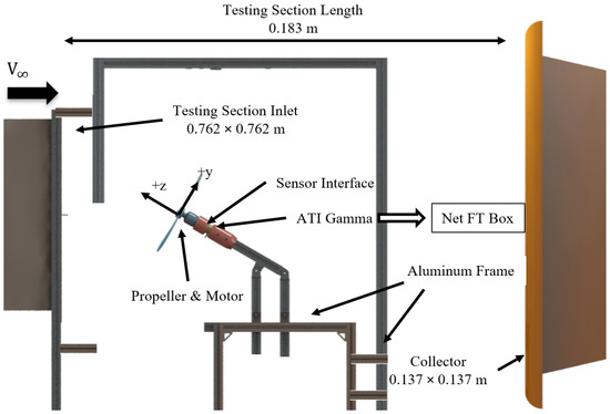
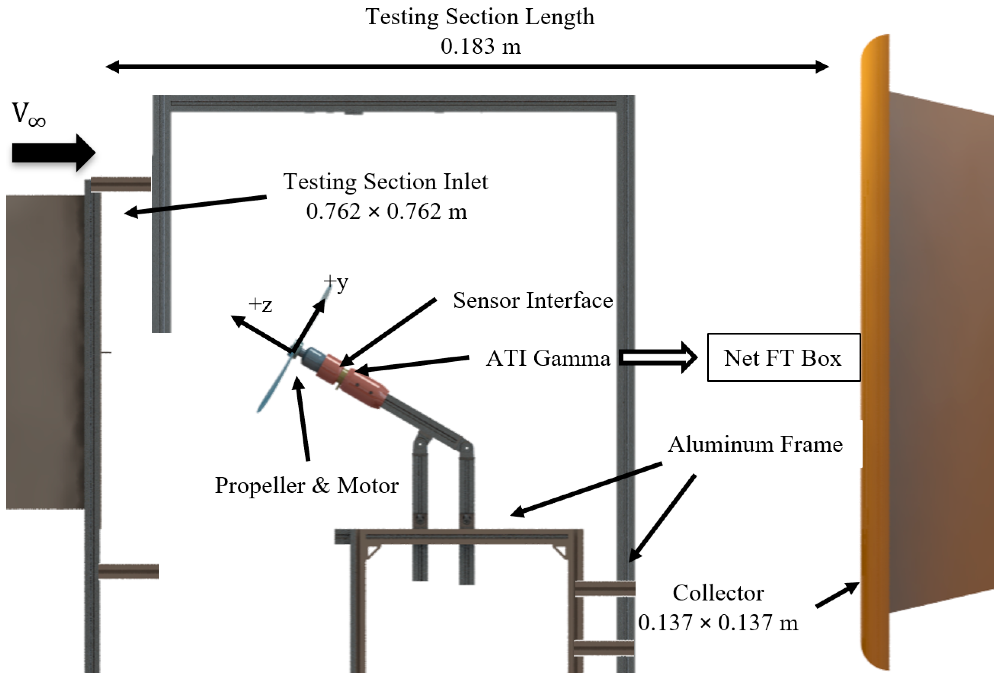
The experimental setup was similar to that in the previous study [7], with a schematic shown in Figure 1. The propeller motor was attached to an ATI Industrial Automation Mini-40 six-component force balance [19]. The axial force along the z-axis is defined as thrust, and the rotational moment about the z-axis as torque. The propeller power coefficient was calculated directly from the measured propeller torque, rather than from the power supply output, to eliminate losses due to heat generation. The balance was bolted to an aluminum extrusion frame secured at the inlet of the plenum. It had a maximum range of 120 N for force on its Z-axis. The peak thrust encountered during the experiment was 25 N. The relative uncertainty of the force balance is 1% of the force reading on the Z-axis according to the manufacturer’s calibration report [19]. The freestream velocity was measured using a TSI pitot tube mounted at the exit of the wind tunnel contraction and recorded by a TSI 5825 Micromanometer. The propeller’s rotational speed was measured with a 50 mW laser and a Thor Labs PDA10A photodiode. Based on the Kline-McClintock uncertainty calculations [20], the average instrument uncertainty is calculated to be 1.22%, based on the measured thrust for the APC 11 × 7 propeller at its medium forward flight speed under 100 RPS (6000 RPM) at 10 m/s forward flight speed.

Figure 1. Schematic of the experimental setup at the University of Dayton Low-Speed Wind Tunnel (UD-LSWT).

All data were sampled at a rate of 1000 Hz for a duration of 15 s at each data point. Two trials were conducted for each case to ensure data repeatability. To minimize sensor drift, tare values were recorded before and after each test with the propeller powered off. The average of the two tare readings was subtracted from the corresponding thrust and torque measurements. If the difference between the tare values before and after tare subtraction exceeded 0.1 N of force on any axis, the experimental data were discarded, and the experiments were repeated. To eliminate the vibration frequency caused by the propeller rotation, uneven blade loading in edgewise flight, and the natural frequency of the aluminum test frame, a Finite Impulse Response (FIR) band-stop filter [21] was applied to the data. The difference between the calculated mean force and moment before and after the data filtration is less than 0.2%. The natural frequency of the aluminum frame was identified by a tap test during our previous study [7] and found to be ~130 Hz. The selected propeller rotational speeds for the experiment are below this value to minimize additional noise in the data collection. The highest average random uncertainty in the force measurements, based on the measured two standard deviations (or 95% confidence interval), is ±9.4% across all the advance ratios tested for all the propellers after data reduction and filtration. The highest uncertainty occurs at the pure edgewise flight condition ($\theta =90°$) and higher forward flight speed ($J>0.5$), mainly due to the uneven blade loading under such conditions. Overall, the results demonstrated excellent repeatability across both experimental runs for all the experiments.

As this study focuses on propeller performance, the axial thrust coefficient is defined according to the propeller conventions developed by McCormick [22] as shown in Equation (1).

$$C_{T_A}={\displaystyle \frac{T_A}{\rho n^2{D}^4}}$$

(1)

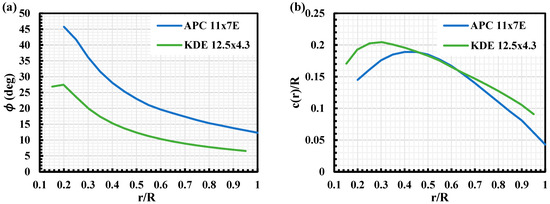
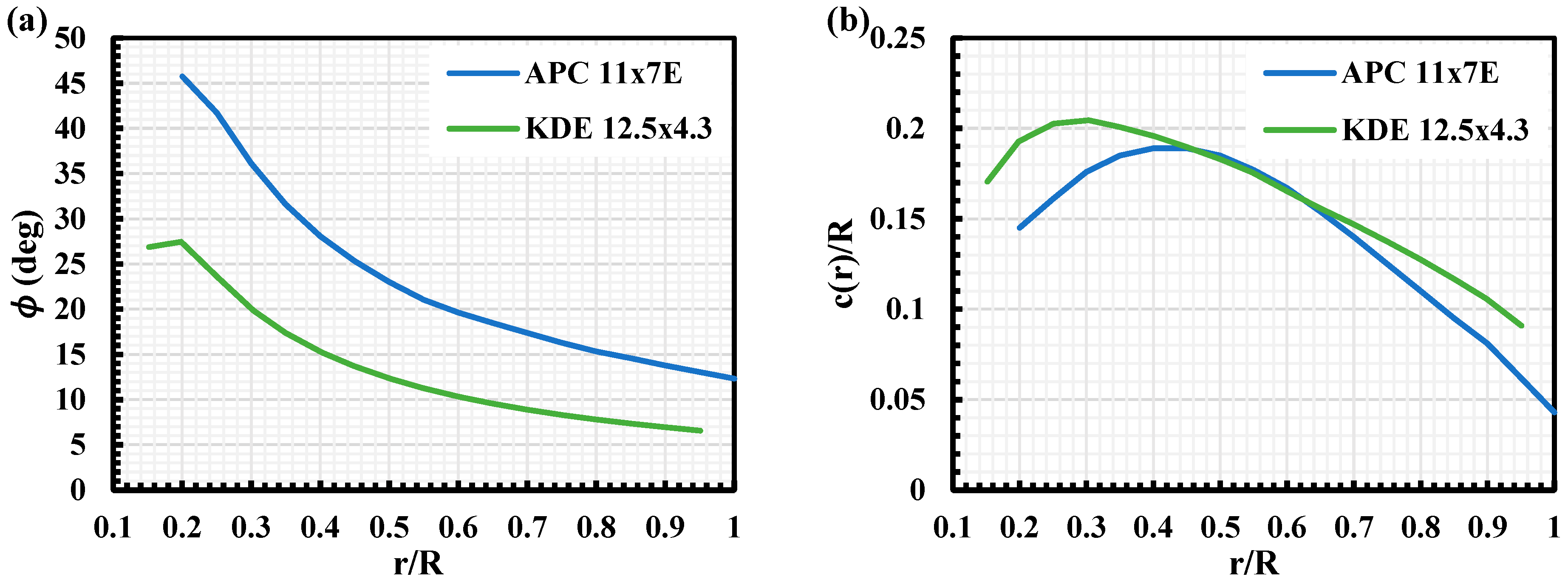
The test matrix for the standalone propeller performance experiment is shown in Table 1. Two different propellers were tested: the KDE [23] 12.5 × 4.3 carbon fiber propeller and the APC [24] 11 × 7E glass-filled nylon propeller, chosen due to differences in their local pitch angle $\left(\varphi \right)$ distribution and local blade chord $\left(c\right(r\left)\right)$ distribution, as depicted in Figure 2. Both propellers are selected with a diameter less than 50% of the wind tunnel test section height and placed at the centerline of the test section to avoid any proximity effect from the edge of the wind tunnel [25,26]. Both propeller blade geometries are obtained directly from the manufacturer. The peak Reynolds number was calculated at the 75% propeller radius. The propeller incidence angles, which are the angle between the plane of incoming freestream and the propeller axial thrust along its shaft axis as seen in Figure 1, range from 0 to 90 degrees. For each rotational speed tested, the wind tunnel freestream velocity was varied to achieve an advance ratio ranging from 0 to 0.7.

Table 1. Test matrix.

Propeller	Rotational Speed per Second ($\mathit{n}$)	Peak Reynolds Number (×1000)	Advance Ratio ($\mathit{J}$)	Incidence Angle $\mathit{\theta }$ (Deg)	Freestream Velocity ${\mathit{V}}_{\mathbf{\infty }}$ (m/s)	${\mathit{V}}_{\mathbf{\infty }}$ Increment (m/s)
KDE 12.5 × 4.3	83.3~116.6	145	0~0.7	0, 30, 45, 60, 75, 90	0~20	1.25
APC 11 × 7E		90

Figure 2. (a) Local blade pitch angle ($\varphi$) distribution for APC and KDE propellers tested; (b) local blade chord ($c\left(r\right)$) distribution for APC and KDE propellers tested.

3. Experimental Results

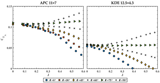
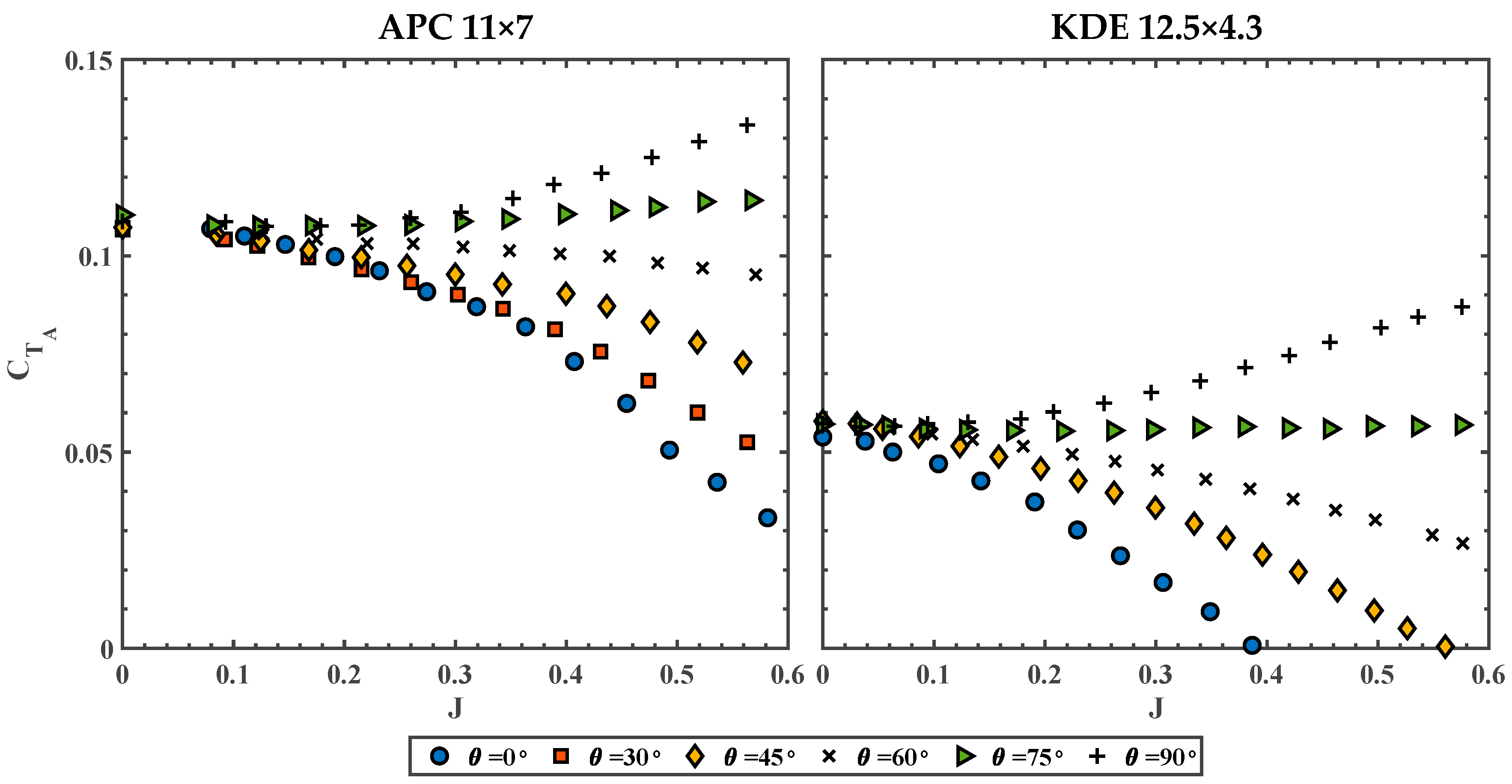
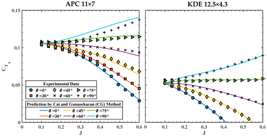
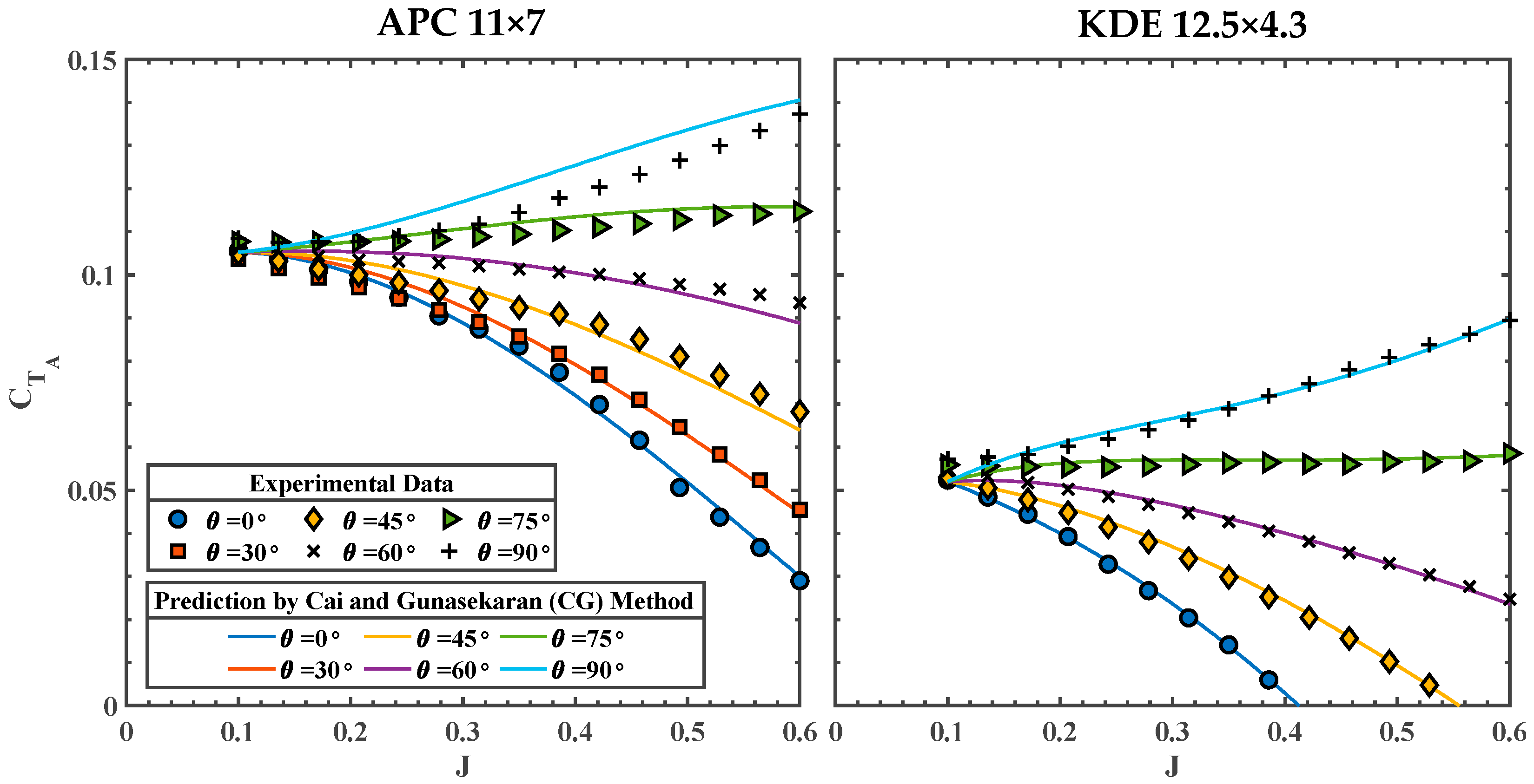
The axial thrust coefficient, $C_{TA}$, vs. advance ratio, $J$, for the APC 11 × 7 and KDE 12.5 × 4.3 propellers, both operating at 100 RPS (6000 RPM), under various $\theta$ is shown in Figure 3. The results align with the trend found in References [4,5,6]: $C_{TA}$ decreases with an increase in $J$ for $\theta$ less than 60$°$. Axial thrust coefficient ($C_{TA}$) increases with $\theta$ at a given $J$. The relationship between $C_{TA}$ and $J$ changes at approximately $\theta ~60°$, where $C_{TA}$ begins to increase with $J$. Despite noticeable differences in geometry (Figure 2), the overall trend for both propellers is similar, although the KDE 12.5 × 4.3 propeller records a lower $C_{TA}$ magnitude due to its lower propeller pitch ($\gamma$).

Figure 3. ${\mathrm{C}}_{\mathrm{T}\mathrm{A}} \mathrm{v}\mathrm{s}. \mathrm{J}$ at various $\mathrm{\theta }$ for APC 11 × 7 (left) and KDE 12.5 × 4.3 (right) under 100 RPS.

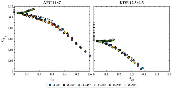
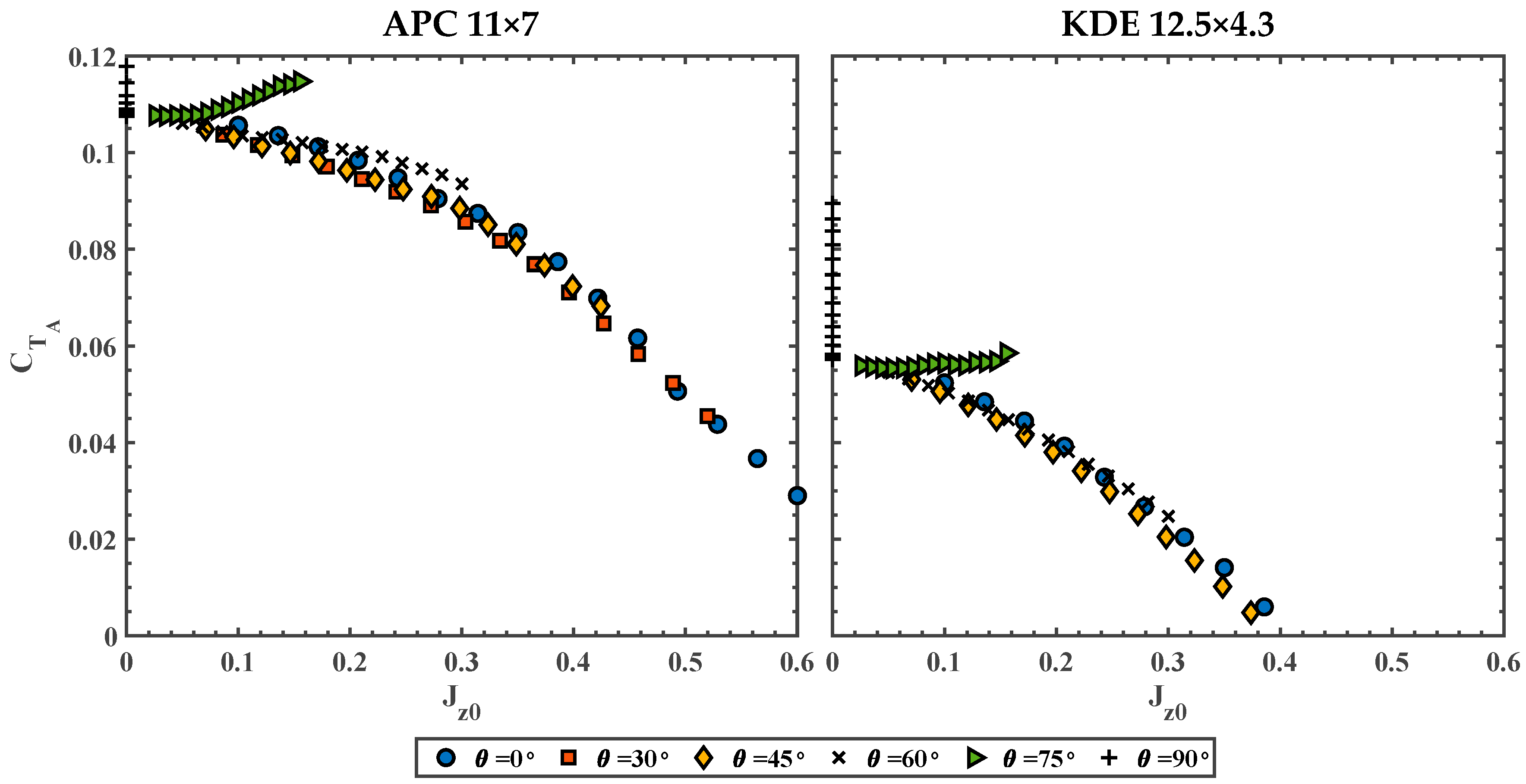
Using a normalized advance ratio, $J_{z0}$, defined in Equation (2) and referenced in [4,5,6,7], Figure 4 replots the results from Figure 3, but with $J_{z0}$ as the independent axis.

$$J_{z0}={\displaystyle \frac{Vcos\theta }{nD}}=J\cos \theta$$

(2)

Figure 4. $C_{TA}$ vs. $J_{z0}$ at various $\mathrm{\theta }$ for APC 11 × 7 (left) and KDE 12.5 × 4.3 (right) under 100 RPS.

The axial thrust coefficient curves collapse at $\theta \le 60°$, indicating that the prediction of performance at $\theta \le 60°$ can be conducted using the data from $\theta =0°$. At $\theta >60°$, the curves do not collapse as effectively, and the approach becomes meaningless at $\theta =90°$. Therefore, a practical method needs to be developed to better estimate the propeller axial thrust at higher incidence angles.

From Figure 4, as all the curves collapse at $\theta \le 60°$, mathematically,

$${\left[C_{T_A}\left(J_{z0}\right)\right]}_{0°\le {\theta }_x\le 60°}\approx {\left[C_{T_A}\left(J\right)\right]}_{\theta =0°}$$

(3)

where ${\left[C_{T_A}\left(J_{z0}\right)\right]}_{{\theta }_x}$ represents $C_{T_A}$ at $\theta$ plotted in terms of $J_{z0}$. Writing in terms of $J$,

$${\left[C_{T_A}\left(J\right)\right]}_{0°\le {\theta }_x\le 60°}\approx {\left[C_{T_A}\left(J_{z0}\right)\right]}_{\theta =0°}={\left[C_{T_A}\left(J\cos \theta \right)\right]}_{\theta =0°}$$

(4)

In general terms,

$${\left[C_{T_A}\left(J\right)\right]}_{\theta ={\theta }_x}\approx {\left[C_{T_A}\left(J\cos \theta \right)\right]}_{\theta =0°}=\mathrm{f}\mathrm{o}\mathrm{r}0°\le {\theta }_x\le 60°$$

(5)

where ${\theta }_x$ represents any incidence angle of choice between $0°$ and $60°$. For example, if ${\left[C_{T_A}\left(J\right)\right]}_{\theta =60°}$ is desired,

$${\left[C_{T_A}\left(J\right)\right]}_{\theta =60°}\approx {\left[C_{T_A}\left(Jcos60°\right)\right]}_{\theta =0°}$$

(6)

By evaluating the $\theta =0°C_{T_A}$ at $J_{z0}/\cos 60°$, $C_{T_A}$ at $\theta =60°$ can be obtained. The equivalency will only work for $0°\le {\theta }_x\le 60°$ as shown in Figure 4. For predicting $C_{T_A}$ at $\theta >60°$, a new approach is required, which will be discussed in the next section.

4. Proposed Axial Thrust Prediction Model

Inspired by the concept of separating propeller performance into propeller-like and wing-like components, terminologies coined by Rubin [10], a new prediction model for propeller axial thrust, distinctly different from the method proposed by Rubin [10], is introduced in the current study.

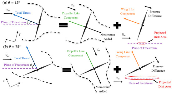
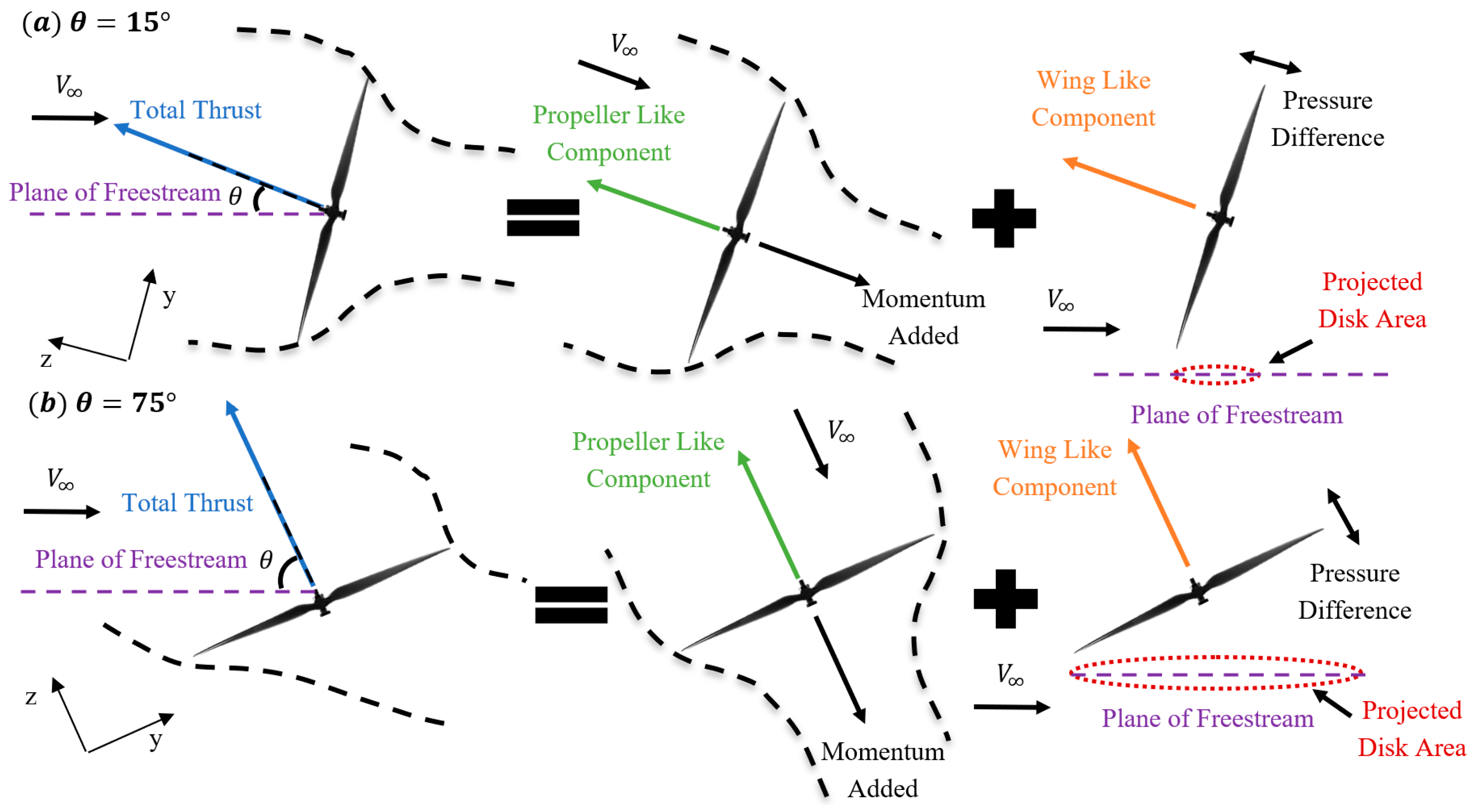
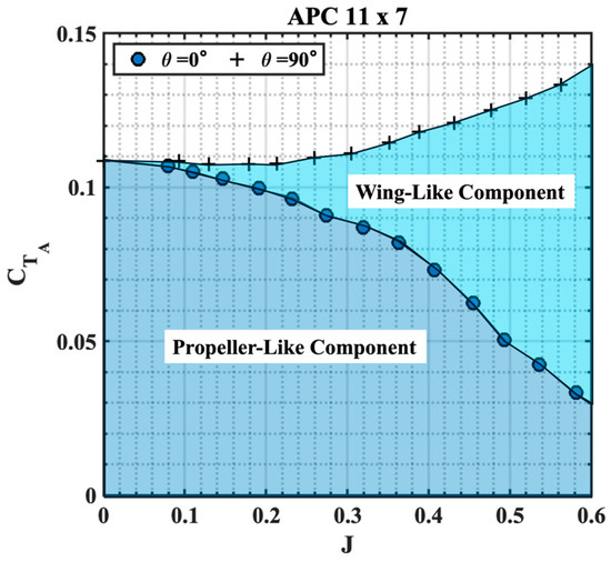
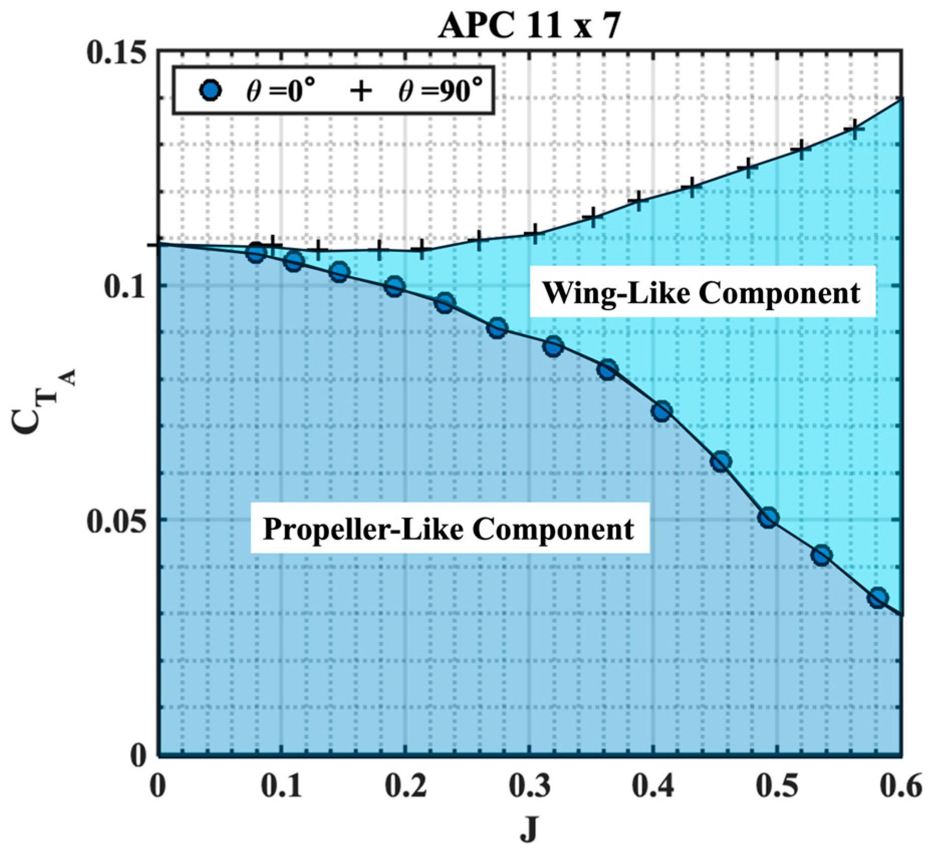
The total axial thrust generated by the propeller at a given forward speed can be considered as the sum of the thrust ($T_A$) generated by the propeller-like component ($T_{Prop}$) and the wing-like component ($T_{Wing}$). The thrust from the propeller-like component is a result of the momentum added to the freestream, similar to the propeller’s axial flight performance at $\theta =0°$, and is assumed to remain constant across different $\theta$ values. The wing-like component treats the propeller disk as a circular plate, where the thrust is generated by the pressure difference between the lower and upper surfaces of the propeller disk, similar to the lift produced by a wing, which creates additional downwash. This is also illustrated in the schematic in Figure 5 for two different incidence angles. In this model, only the projected area of the propeller disk on the plane of freestream is considered for the wing component, and it will vary at different incidence angles. Consequently, this component is zero at $\theta =0°$ and increases with an increase in $\theta$. The experimental result from the APC 11 × 7 propeller at $\theta =0°$ and $\theta =90°$ is used to demonstrate the concept of the wing-like and propeller-like thrust components, as shown in Figure 6.

Figure 5. Schematic illustrating the propeller-like and wing-like components at (a) θ = 15° and (b) θ = 75°.

Figure 6. Example $C_{TA}\mathrm{v}\mathrm{s}.J$ illustrating the propeller-like and wing-like thrust components.

The dark blue shaded area represents $C_{TA}\mathrm{v}\mathrm{s}.J$ at $\theta =0°$ (indicated by circular markers) which represents the propeller-like component. As the incidence angle increases, the projected area of the propeller disk also increases, resulting in the wing-like component thrust ($C_{T_{Wing}}$). For the $\theta =90°$ case (indicated by cross markers), the additional thrust generated by the propeller, compared to the $\theta =0°$ case, is hypothesized to be a result of the wing-like component, which is marked in light blue shade. Generalizing this hypothesis,

$${\left[C_{T_A}\right]}_{\theta ={\theta }_x}=\underset{\begin{array}{c}Propeller-like\\ Component\end{array}}{\underbrace{{\left[C_{T_A}\right]}_{\theta =0°}}}+\underset{\begin{array}{c}Wing-like\\ Component\end{array}}{\underbrace{{\left[C_{T_{Wing}}\right]}_{\theta ={\theta }_x}}}$$

(7)

Note that for $0°\le {\theta }_x\le 60°$, $C_{T_{Wing}}$ is predictable using the normalized $J_{z0}$ approach discussed in the previous section and Equations (2)–(6). $C_{T_{Wing}}$ for $0°\le {\theta }_x\le 60°$ can be written as,

$${\left[C_{T_{Wing}}\right]}_{\theta ={\theta }_x}={\left[C_{T_A}\left(J\right)\right]}_{\theta ={\theta }_x}-{\left[C_{T_A}\left(J\right)\right]}_{\theta =0°}$$

(8)

Using Equation (5), we can write,

$${\left[C_{T_{Wing}}\right]}_{\theta ={\theta }_x}={\left[C_{T_A}\left(J\cos {\theta }_x\right)\right]}_{\theta =0°}-{\left[C_{T_A}\left(Jcos0°\right)\right]}_{\theta =0°}\mathrm{f}\mathrm{o}\mathrm{r}0°\le {\theta }_x\le 60°$$

(9)

For example, if $C_{T_{Wing}}$ at $\theta =60°$ is desired,

$${\left[C_{T_{Wing}}\right]}_{\theta =60°}={\left[C_{T_A}\left(J\cos 60°\right)\right]}_{\theta =0°}-{\left[C_{T_A}\left(J\right)\right]}_{\theta =0°}$$

(10)

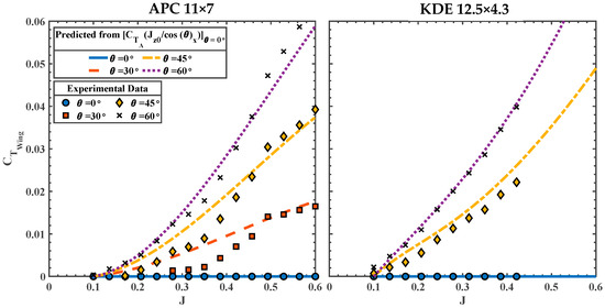
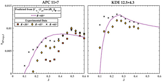
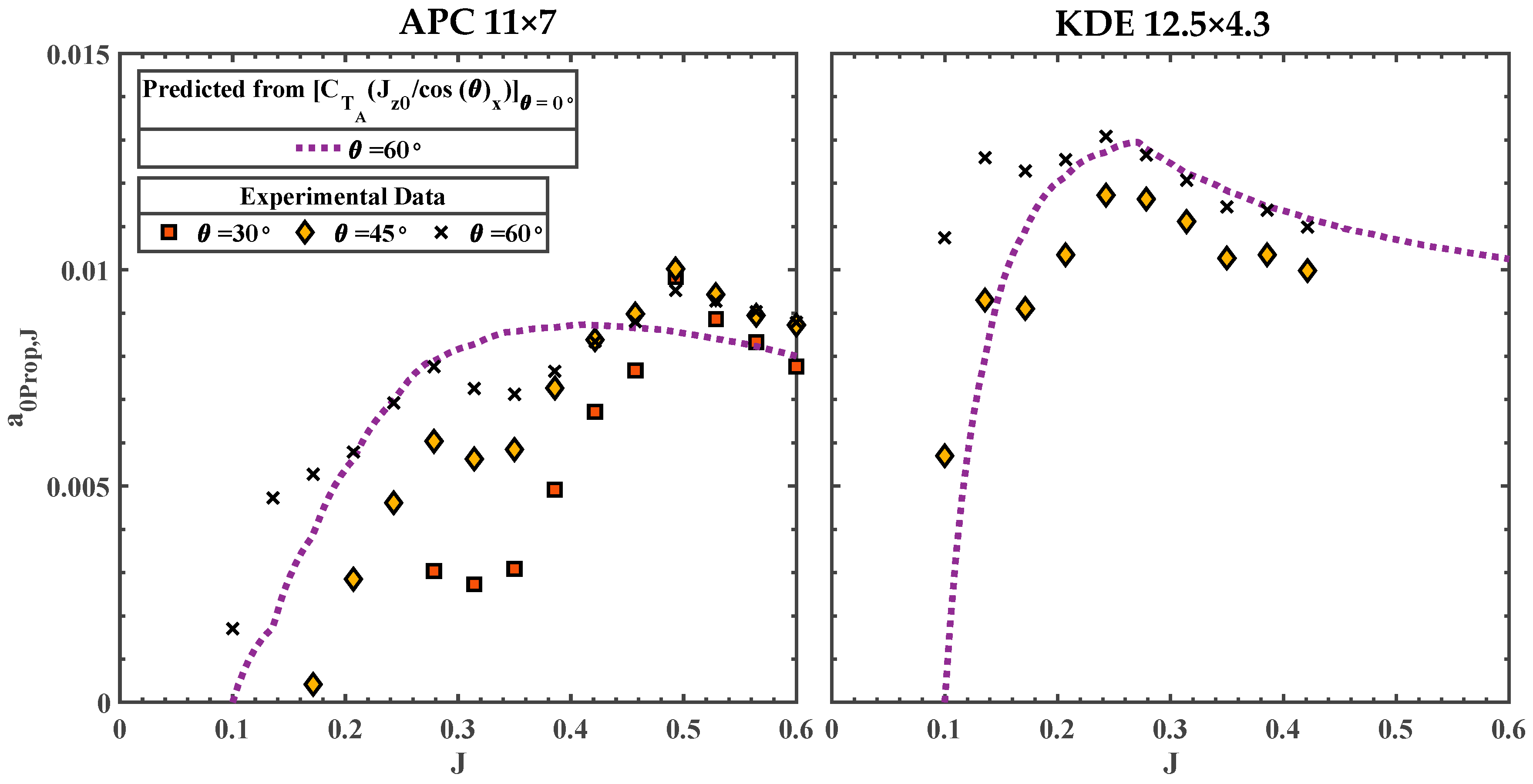
The variation of $C_{T_{Wing}}$ at different incidence angles is shown in Figure 7 for both APC and KDE propellers derived from experimental data and the $J_{z0}$ normalization approach discussed above.

Figure 7. $C_{T_{Wing}}$ vs. $J$ at different $\theta$ for APC 11 × 7 (left) and KDE 12.5 × 4.3 (right).

Good agreement between the predicted $C_{T_{Wing}}$ and experiment is observed in the KDE propeller, whereas the agreement between the experiment and prediction suffers at lower J for the APC propeller at lower incidence angles. The $J_{z0}$ normalization method overpredicts $C_{T_{Wing}}$ for the $\theta =30°$ and $\theta =45°$ cases in the range of $0.2\le J\le 0.5$. At $J>0.5$, the prediction and the experiment align well. This variation could be due to blade flow separation at lower $J$ at the incidence angle, caused by the high blade pitch. At $\theta =60°$, both propellers show good agreement between the prediction and the experiment, a result that will be extremely valuable to the analysis later on. As mentioned above, this approach to predicting $C_{T_A}$ only works for $0°\le {\theta }_x\le 60°$. The $J_{z0}$ normalization diverges from ${\left[C_{T_A}\left(J_{z0}\right)\right]}_{\theta =0°}$ at $\theta >60°$. Therefore, a different, more generalized method must be used for predicting $C_{T_{Wing}}$ and $C_{T_A}$, which will be discussed below. The generic equation to predict lift from a wing can be expressed as,

$$L={\displaystyle \frac{1}{2}}\rho V_{\infty }^{2}S{C}_L$$

(11)

where the coefficient of lift is expressed as,

$$C_L=a_0\alpha$$

(12)

where $a_0$ represents the lift curve slope of the wing, and $\alpha$ is the angle of attack. Considering that the wing-like component of propeller thrust generates lift in a similar manner, with a pressure difference across the propeller disk, Equation (11) can be adapted for a propeller to model this wing-like component. We replace the wing reference area $S$ with the propeller’s freestream projected area, $S\sin \theta$, in Equation (11) and introduce a lift coefficient of the propeller disk, ${C_L}_{Prop}$, instead of the wing lift coefficient $C_L$. Making this substitution and using the traditional thrust equation defined by McCormick [22] gives:

$$T_{Wing}={\displaystyle \frac{1}{2}}\rho V_{\infty }^2\left(Ssin\theta \right)C_{Lprop}=C_{Twing}\rho n^2{D}^4$$

(13)

Canceling the common terms on the left-hand side and the right-hand side of Equation (13) and rewriting $V_{\infty }$ in terms of $JnD$, yields:

$${\displaystyle \frac{1}{2}}{J}^2\left(Ssin\theta \right)C_{Lprop}=C_{Twing}{D}^2$$

(14)

Using the propeller disk area $S={\displaystyle \frac{1}{4}}\pi D^2$ and canceling out the terms on both sides of Equation (14), an expression for $C_{Twing}$ can be obtained as:

$$C_{Twing}={\displaystyle \frac{1}{8}}\pi J^{2}sin\theta C_{LProp}$$

(15)

where $C_{LProp}$ is a function of $\theta$, similar to the angle of attack for a wing, and remains constant at each $J$. $C_{LProp}$ can vary with the changes in $J$, analogous to the Reynolds number effect on a wing. $C_{LProp}$ also differs for each propeller, similar to how different airfoils affect the wing’s performance. An analogous expression to $C_L$ in Equation (12) can be written for $C_{LProp,J}$ as:

$$C_{LProp,J}=a_{0prop,J}{\theta }^k$$

(16)

where $a_{0prop,J}$ is the analogous ‘lift curve slope’ for the propeller disk at advance ratio $J$ and $k$ is a non-linear factor, which will be discussed later in the section. Substituting Equation (16) into Equation (15) yields:

$$C_{Twing}={\displaystyle \frac{1}{8}}\pi J^{2}sin\theta a_{0prop,J}{\theta }^k$$

(17)

Therefore, to calculate $C_{TWing}$ at a given $\theta$, $a_{0prop,J}$ at each advance ratio, or $a_{0prop,J}\mathrm{v}\mathrm{s}.J$, needs to be found. To probe the characteristics of $C_{LProp,J}$ and $a_{0prop,J}$, known values of $C_{T_{Wing}}$ can be used. Recall from Equation (9) that $C_{T_{Wing}}$ at any $0°\le {\theta }_x\le 60°$ can be estimated using the $J_{z0}$ normalization approach. Therefore, solving for $C_{LProp,J}$ for $0°\le {\theta }_x\le 60°$,

$$C_{LProp,J}=8{\displaystyle \frac{{\left[C_{T_{Wing}}\right]}_{\theta ={\theta }_x}}{\pi J^2\left(\mathit{sin}{\theta }_x\right)}}$$

(18)

Substituting Equation (9) into Equation (18),

$$C_{LProp,J}=8{\displaystyle \frac{\left[{\left[C_{T_A}\left(J\cos {\theta }_x\right)\right]}_{\theta =0°}-{\left[C_{T_A}\left(J\right)\right]}_{\theta =0°}\right]}{\pi J^2\left(\mathit{sin}{\theta }_x\right)}}(0°<{\theta }_x\le 60°)$$

(19)

For example, $C_{LProp,J}$ at $\theta =60°$ can be calculated as,

$$C_{LProp,J}=8{\displaystyle \frac{\left[{\left[C_{T_A}\left(J\cos 60°\right)\right]}_{\theta =0°}-{\left[C_{T_A}\left(J\right)\right]}_{\theta =0°}\right]}{\pi J^2\left(\mathit{sin}60°\right)}}$$

(20)

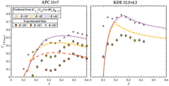
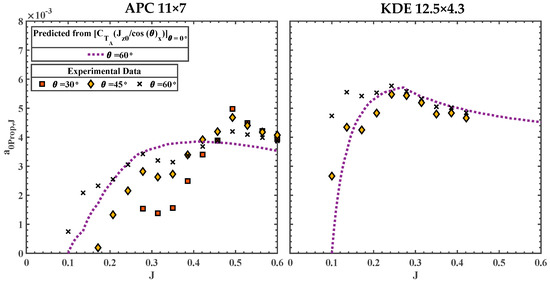
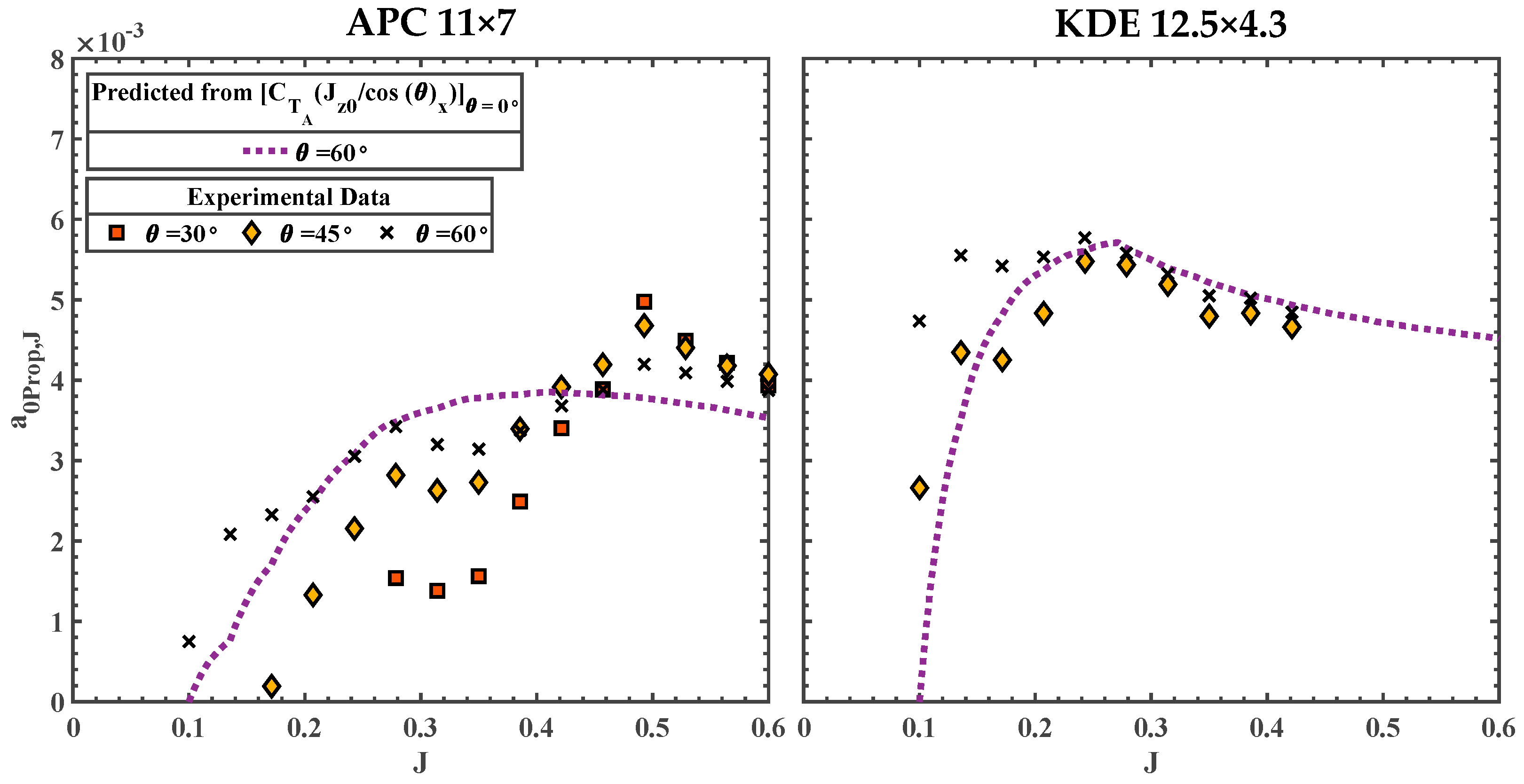
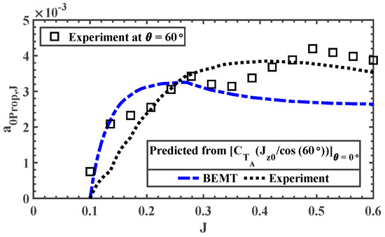
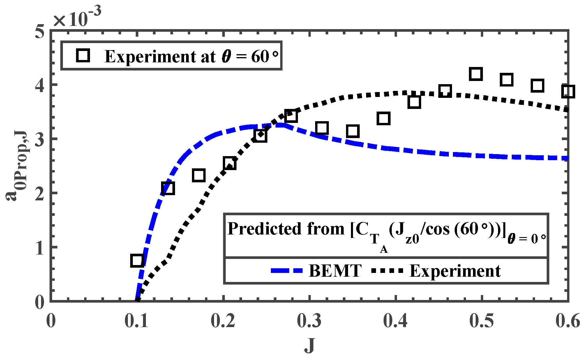
The comparison of the predicted and experimental $C_{LProp,J}$ at different incidence angles is shown in Figure 8. The trends in $C_{LProp,J}$ are remarkably similar to those observed for a finite wing. The comparison between the prediction and experiments follows similarly to the comparisons observed in $C_{T_{Wing}}$ in Figure 7. Drastic deviations are observed at lower $J$ for $\theta =30°$ and $\theta =45°$ cases in the range of $0.2\le J\le 0.5$. At $J>0.5$, the prediction and the experiment agree well. Once again, this deviation could be due to the flow separation caused at lower $J$ at the incidence angle. At $\theta =60°$, both the propellers show good agreement between the prediction and the experiment.

Figure 8. Comparison of the predicted and experimentally obtained ${\mathit{C}}_{\mathit{L}\mathit{P}\mathit{r}\mathit{o}\mathit{p},\mathit{J}}$ at various $\mathit{\theta }$.

The $C_{LProp,J}$ magnitude in Figure 8 shows an incremental change with the increase in $\theta$, and the magnitude variation with $J$ is relatively similar across all $\theta$. Therefore, according to the definition of $C_{LProp,J}$ introduced in Equation (16), $a_{0prop,J}$ should be relatively constant for all $\theta$ and should preserve the trend across all $J$. Solving for $a_{0prop,J}$ from Equation (16) yields:

$$a_{0prop,J}=C_{LProp,J}/{\theta }^k$$

(21)

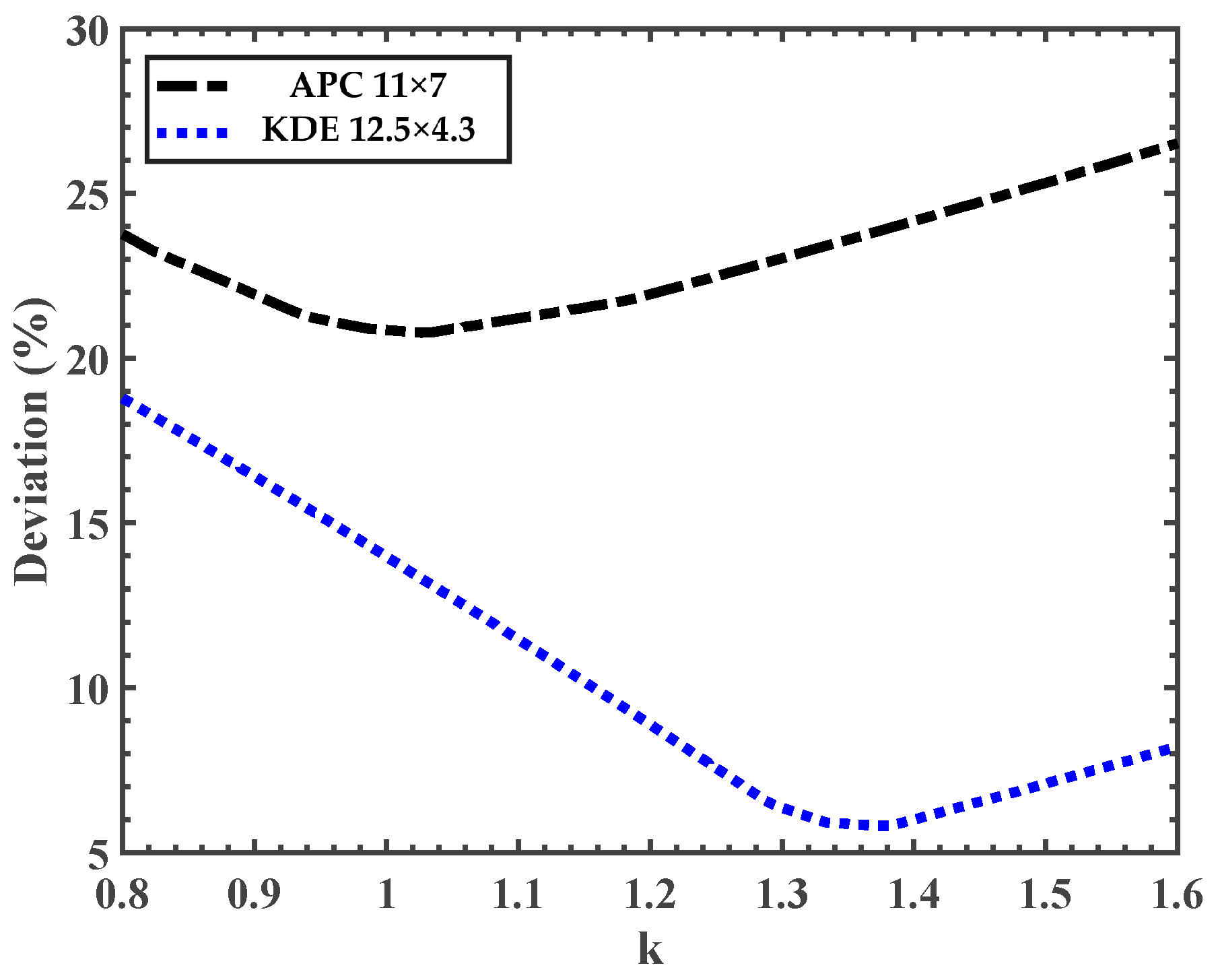
The $a_{0prop,J}$ created with $k=1$ is shown in Figure 9. Almost all the experimental cases collapse on each other for both propellers, except for $\theta =30°$ case at $J<0.4$. This collapse is essential for the $a_{0prop,J}$ to be independent of $\theta$. To identify the non-linear factor $k$ that would result in the best collapse of the $a_{0prop,J}$ curves, error analysis was conducted to determine the value of $k$ that would achieve the best possible collapse of the experimental data. Two incidence angle cases, $\theta =45°$ and $\theta =60°$ were used in this analysis. The average percentage deviation was defined as

$$AverageDeviation\left(\%\right)=\overline{{\displaystyle \frac{{\left[a_{0prop,J}\right]}_{\theta =60°}-{\left[a_{0prop,J}\right]}_{\theta =45°}}{{\left[a_{0prop,J}\right]}_{\theta =60°}}}}\ast 100$$

(22)

Figure 9. Comparison of the predicted (using $k=1$) and experimentally obtained $a_{0prop,J}$.

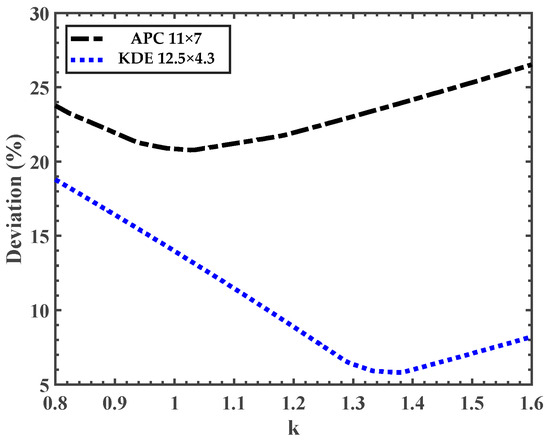
The result from the percentage deviation analysis is shown in Figure 10. The best collapse for the case of the APC 11 × 7 propeller was achieved around $k~1$, whereas for the KDE propeller, it was achieved at $k~1.3$. The overall deviation between the two $a_{0prop,J}$ cases differs between the two propellers, with the KDE propeller showing the lowest percentage deviation.

Figure 10. Percentage deviation of the estimated $a_{0prop,J}$ vs. non-linear factor $k$.

The varying dependency of $C_{LProp,J}$ with $\theta$, and hence different $k$ for different propellers, is not surprising. Several factors, such as blade twist and chord distribution, could affect this dependency. Given that the two propellers chosen for the study are drastically different in terms of pitch, diameter, twist, and chord distributions, the overall deviations in $k$ are relatively minimal. On the other hand, a lower pitch-to-diameter ratio propeller, which is more favorable when operating at higher incidence angles and in edgewise flight, has better blade lift/thrust generation capabilities than a higher pitch-to-diameter ratio propeller, which is usually designed for higher-speed axial flight. Therefore, the propeller designed for edgewise flight would yield a higher $a_0$, as observed in Figure 9.

A more generalized approach would be to choose a $k$ value that does not perfectly collapse the $a_{0prop,J}$ curves for either of the propellers. Therefore, all further analysis was conducted with a $k$ value of 1.2, as an empirical compromise for the two propellers studied here. It is worth noting that this k value is obtained using the incidence angle in the unit of degrees, instead of rad. The resultant $a_{0prop,J}$ with $k=1.2$ is plotted in Figure 11 and shows a reasonable collapse of the experimental data, removing the influence of $\theta$ on $a_{0prop,J}$. As such, only one estimate of $a_{0prop,J}$ is required to predict the variation of $a_{0prop,J}$ with $J$ for all $\theta$. It can be observed in Figure 10 that the $a_{0prop,J}$ predicted using the $J_{z0}$ normalized method at $\theta =60°$ captures the general trend with $J$ for both the propellers. Thus, this $a_{0prop,J}$ predicted at $\theta =60°$ using the $J_{z0}$ normalized method can be assumed constant for all $0°\le {\theta }_x\le 90°$.

Figure 11. Comparison of the predicted (using $k=1.2$) and experimentally obtained $a_{0prop,J}$ for both propellers.

Therefore, the propeller axial thrust coefficient at any given ${\theta }_x$ in the range of $0°\le {\theta }_x\le 90°$ can be calculated as:

$${\left[C_{T_A}\right]}_{\theta ={\theta }_x}=\underset{\begin{array}{c}Propeller-like\\ Component\end{array}}{\underbrace{{\left[C_{T_A}\right]}_{\theta =0°}}}+\underset{\begin{array}{c}Wing-like\\ Component\end{array}}{\underbrace{{\left[C_{T_{Wing}}\right]}_{\theta ={\theta }_x}}}={\left[C_{T_A}\right]}_{\theta =0°}+{\displaystyle \frac{1}{8}}\pi J^2\left(sin\theta \right)a_{0prop,J}{\theta }^k$$

(23)

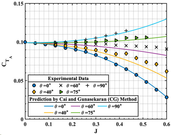
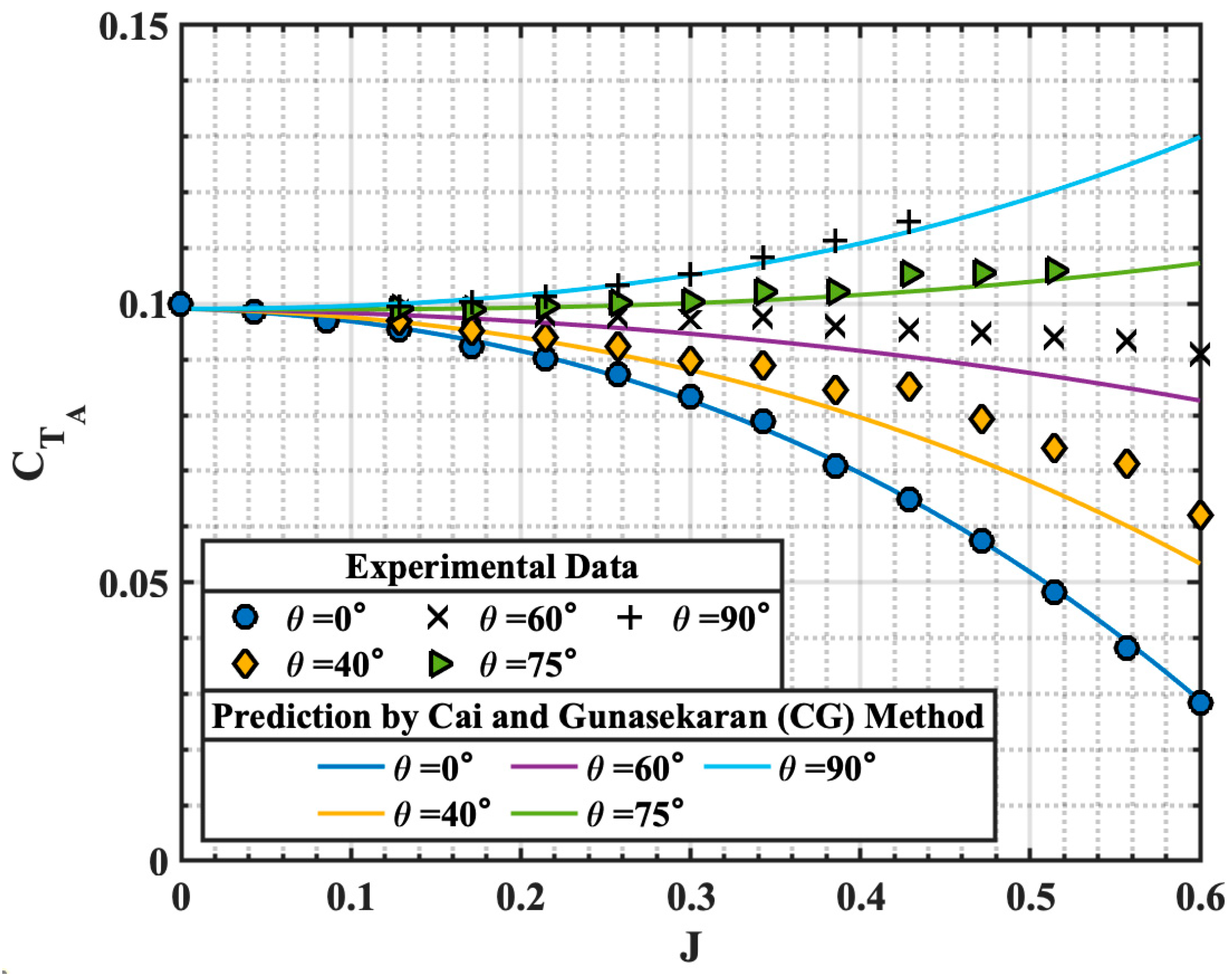
with $a_{0prop,J}$ determined using Equations (20) and (21). A $k$ value of 1.2 would result in a reasonable estimate which can be further tuned if experimental data at any non-zero incidence angle were available. The $C_{T_A}$ predicted by the proposed method is compared with the experimental data in Figure 12 for various incidence angles. Larger deviations from the experiments were observed in the APC propeller at $\theta =90°$, where the method slightly overpredicts the axial thrust generated. However, the proposed prediction method shows relatively good agreement with the experimental results for both propellers across all the incidence angles, with an average relative error of 8.3%, calculated at each advance ratio using the axial flight experimental data method.

Figure 12. Comparison of the APC 11 × 7 (left) and KDE 12.5 × 4.3 (right) propeller experimental results and proposed $C_{Tz}\mathrm{v}\mathrm{s}.J$ prediction methods.

5. Summary of the Prediction Method

This section summarizes the overall proposed prediction method using a step-by-step approach to predict the propeller thrust coefficient from $0°$ to $90°$ using the propeller performance data at $\theta =0°$.

Step 1: Obtain ${{\mathit{C}}_{\mathit{T}}}_{\mathit{A}}$ vs. $\mathit{J}$ data at $\mathit{\theta }\mathbf{=}\mathbf{0}\mathbf{°}$.

The key input for the prediction method is the propeller ${C_T}_A$ vs. $J$ data at $\theta =0°$. Therefore, the first step in the prediction method is to obtain $C_{T_A}$ at $\theta =0°$.

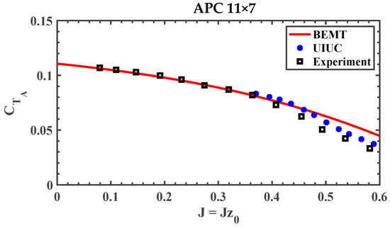
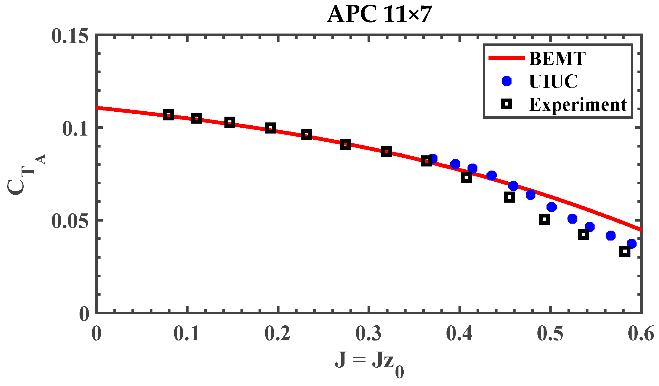
This data can be obtained by the BEMT method [8], numerical panel methods [9,15], manufacturer data [23,24], or online databases such as the UIUC propeller database [1,2,3]. The use of BEMT eliminates the need for experimental data, allowing for the prediction of $C_{T_A}$ at any $0°\le {\theta }_x\le 90°$ without experimental data. However, if experimental data is available at $\theta =0°$, it is recommended that it be used. A comparison between BEMT (using the Clark-Y as the propeller airfoil based on the manufacturer’s suggestion [24]), experimental data, and the UIUC database at $\theta =0°$ for the APC 11 × 7 propeller is shown in Figure 13.

Figure 13. Comparison of $C_{TA}\mathrm{v}\mathrm{s}.J$ for APC 11 × 7 propeller from different sources [1,2,3,9,24].

Step 2: Predict ${\mathit{C}}_{{\mathit{T}}_{\mathit{A}}}$ at $\mathit{\theta }\mathbf{=}\mathbf{60}\mathbf{°}$ using ${\mathit{J}}_{\mathit{z}\mathbf{0}}$ normalization method.

Since the $\theta \le 60°$ cases reasonably represent the collapse of the $a_{0prop,J}$ curves, we can use the $J_{z0}$ normalization method to predict $C_{T_A}$ and $C_{T_{Wing}}$ at $\theta \le 60°$ by evaluating $C_{T_A}$ at $\theta =0°$ at $J\cos 60°$. It is recommended to select a larger reference incidence angle, ${\theta }_{ref}$, to minimize the overall error in the prediction. Therefore, ${\theta }_{ref}=60°$ is selected for the demonstration. Using Equation (6) and Equation (10), the predicted $C_{T_A}$ and $C_{T_{Wing}}$ at $\theta =60°$ are shown in Figure 14 below.

Figure 14. Experimentally obtained and predicted $C_{T_A}$ and $C_{T_{Wing}}$ at $\theta =60°$.

Once again, the $C_{T_A}$ and $C_{T_{Wing}}$ at $\theta =60°$ predicted by the $J_{Z0}$ normalization method, using experimental $C_{T_A}$ at $\theta =0°$ as an input, match well with experimental data obtained directly at $\theta =60°$. The result predicted using the BEMT input shows a larger deviation from the experimental data at higher $J$.

Step 3: Predict ${\mathit{a}}_{\mathbf{0}\mathit{p}\mathit{r}\mathit{o}\mathit{p},\mathit{J}}$ using calculated ${\mathit{C}}_{{\mathit{T}}_{\mathit{W}\mathit{i}\mathit{n}\mathit{g}}}$.

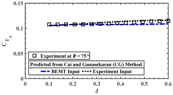
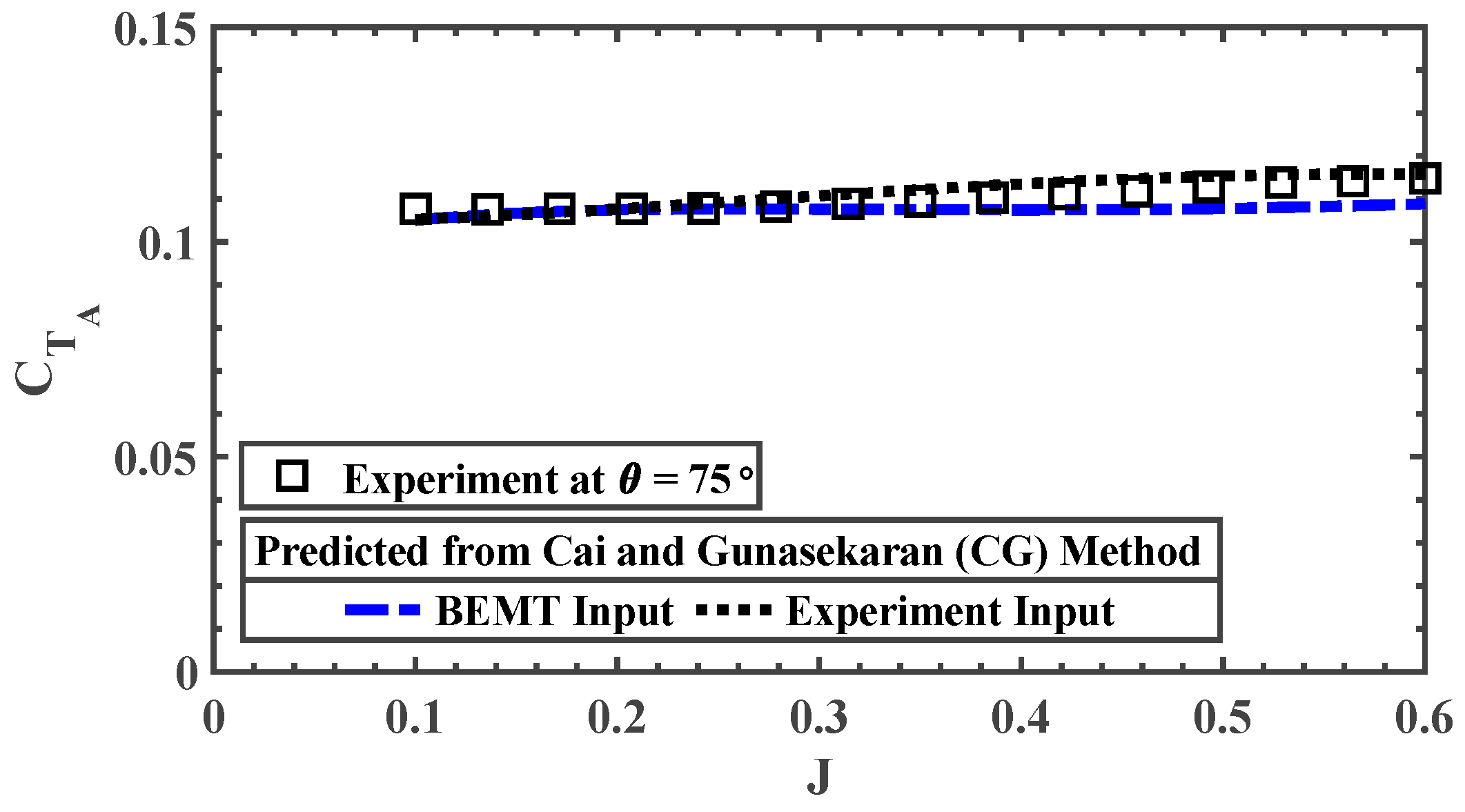
With $C_{T_A}$ and $C_{T_{Wing}}$ at $\theta =60°$ obtained, $a_{0prop}\mathrm{vs}.J$ can be calculated using Equation (21) with $k=1.2$. Figure 15 shows the comparison of $a_{0prop}\mathrm{vs}.J$ between the experiment and predictions using the $\theta =0°$ from BEMT and experiment as inputs. As expected, the $a_{0prop,J}$ predicted by the use of experimental data at $\theta =0°$ aligns well with the $a_{0prop,J}$ obtained directly from the experiment at $\theta =60°$. $a_{0prop}$ can then be used to calculate $C_{T_A}$ in the next step.

Figure 15. Comparison of the experimentally obtained and predicted $a_{0prop}\mathrm{v}\mathrm{s}.J$.

Step 4: Find ${\left[{\mathit{C}}_{{\mathit{T}}_{\mathit{A}}}\left(\mathit{J}\right)\right]}_{\mathit{\theta }={\mathit{\theta }}_{\mathit{x}}}$ for any $\mathbf{0}\mathbf{°}\mathbf{\le }{\mathit{\theta }}_{\mathit{x}}\mathbf{\le }\mathbf{90}\mathbf{°}$.

With $a_{0prop}\mathrm{vs}.J$ estimated, $C_{T_{Wing}}$ at $0°\le {\theta }_x\le 90°$ can be estimated using Equation (17). Combining $C_{T_{Wing}}$ and $C_{TProp}$ (from Step 1), $C_{TA}$ at ${\theta }_x$ can be obtained using Equation (23) when substituting Equations (6), (10), (18)–(21), which yields:

$${\left[C_{T_A}\right]}_{\theta ={\theta }_x}={\left[C_{T_A}\right]}_{\theta =0°}+f\left({\theta }_x\right)\left[{\left[C_{T_A}\left(J\cos {\theta }_{ref}\right)\right]}_{\theta =0°}-{\left[C_{T_A}\left(J\right)\right]}_{\theta =0°}\right]$$

(24)

where $f\left({\theta }_x\right)$ can be expressed as:

$$f\left({\theta }_x\right)={\displaystyle \frac{sin{\theta }_x{\theta }_x^k}{sin{\theta }_{ref}{\theta }_{ref}^k}}={\displaystyle \frac{sin{\theta }_x{\theta }_x^{1.2}}{sin60°{\left(60°\right)}^{1.2}}}$$

(25)

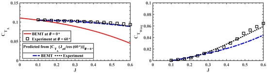
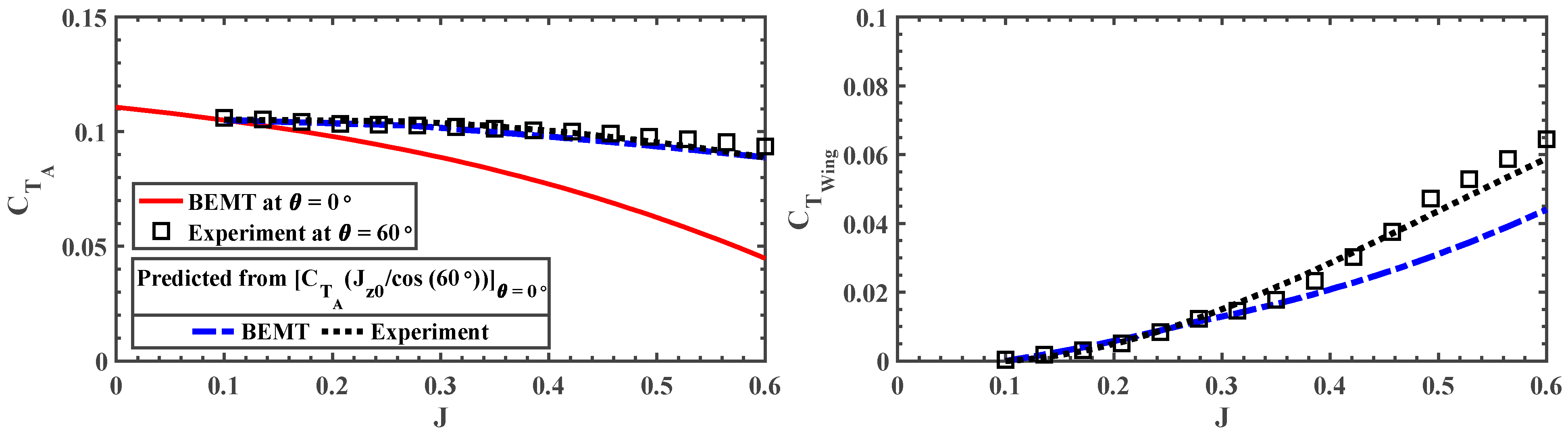
An example of the estimated $C_{TA}$ for the APC 11 × 7 propeller at $\theta =75°$, compared with the experimental results, is shown in Figure 16. The $C_{T_A}$ obtained by the proposed method using BEMT input slightly underpredicts the $C_{T_A}$ when compared to the experimental data. However, the prediction using the proposed method with experimental data as the input agrees well with the experimental results obtained directly at $\theta =75°$.

Figure 16. Comparison of the experimentally obtained and predicted ${\mathit{C}}_{\mathit{T}\mathit{A}}\mathbf{v}\mathbf{s}.\mathit{J}$ for APC 11 × 7 at $\mathit{\theta }\mathbf{=}\mathbf{75}\mathbf{°}$.

Model Validation with Experimental Data from the Literature

The proposed prediction method is then applied to the experimental data for a three-bladed 16 × 8 propeller reported by Simmons and Hatke [4]. The experimental data at $\theta =0°$ was used and the comparison of the proposed model and experimental data is shown in Figure 17. In general, the proposed model shows good agreement with the experimentally obtained results, especially at higher incidence angles. It is worth noting that at $\theta \le 60°$, the prediction model underpredicts the propeller thrust generation at higher $J$ by an average relative error of approximately 7%. This comparison provides an initial test of the model on an additional fixed-pitch propeller. Moreover, it is more applicable to propellers with smaller pitch-to-diameter ratios (Figure 12) that are more commonly used for eVTOL UAVs, which are less likely to experience blade stalls in near-edgewise flight.

Figure 17. Comparison of the experimentally obtained [4] and predicted $C_{TA}\mathrm{v}\mathrm{s}.J$ for the three-bladed 16 × 8 propeller [4].

6. Conclusions

A fast propeller performance prediction method is proposed in this study to estimate a standalone propeller shaft-axis mean thrust generation under various incidence angles between pure axial flight and pure edgewise flight up to an advance ratio of about 0.6. The prediction model considers the propeller performance at higher incidence angles as a summation of the propeller-like thrust component, which remains constant across different incidence angles, and the wing-like thrust component, which varies at different incidence angles. By utilizing reliable propeller performance data from axial flight, which can be obtained from various sources, the model is capable of predicting the propeller performance between axial and edgewise flight using the axial flight data obtained from experiments and validated by the experimental data from the literature. The proposed fast prediction model can be used in the design process of Advanced Air Mobility (AAM) type vehicles to obtain a first-order estimate of the axial thrust coefficient at various advance ratios and tilt angles without an in-depth analysis of the propeller performance, which is beneficial in the air vehicle conceptual design stage.

References

- Brandt, J.B. Small-Scale Propeller Performance at Low Speeds. Master’s Thesis, University of Illinois at Urbana-Champaign, Champaign, IL, USA, 2005. [Google Scholar]
- Deters, R.W. Performance and Slipstream Characteristic of Small-Scale Propellers at Low Reynolds Numbers. Ph.D. Thesis, University of Illinois at Urbana-Champaign, Urbana, IL, USA, 2014. [Google Scholar]
- Dantsker, O.D.; Caccamo, M.; Deters, R.W.; Selig, M.S. Performance Testing of APC Electric Fixed-Blade UAV Propellers. In Proceedings of the AIAA Aviation and Aeronautics Forum and Exposition (Aviation 2022), AIAA Paper 2022-4020, Chicago, IL, USA, 1–27 June 2022. [Google Scholar] [CrossRef] [Scilit]
- Simmons, B.M.; Hatke, D.B. Investigation of High Incidence Angle Propeller Aerodynamics for Subscale eVTOL Aircraft; NASA/TM-20210014010; NASA: Washington, DC, USA, 2021.
- McLemore, H.C.; Cannon, M.D. Aerodynamic Investigation of a Four-Blade Propeller Operating through an Angle of Attack from 0 Degree to 180 Degree; NASA Tech Note 3228; NACA: Washington DC, USA, 1954. [Google Scholar]
- Young, J.D. Propeller at High Incidence. J. Aircr. 1965, 2, 241–250. [Google Scholar] [CrossRef] [Scilit] [PubMed]
- Cai, J.; Gunasekaran, S. Frequency Response of RC Propellers to Streamwise Gusts in Forward Flight. Wind 2023, 3, 253–272. [Google Scholar] [CrossRef] [Scilit]
- Leng, Y.; Jardin, T.; Moschetta, J.-M.; Bronz, M. Analytic Model of Proprotor Forces and Moments at High Incidence. J. Am. Helicopter Soc. 2021, 66, 1–15. [Google Scholar] [CrossRef] [Scilit]
- Leishman, J.G. Principles of Helicopter Aerodynamics; Cambridge University Press: Cambridge, UK, 2006; pp. 115–169. [Google Scholar]
- Rubin, R.L. Theoretical and Experimental Aerodynamic Thrust Studies of Propellers at Angles of Incidence. Ph.D. Thesis, University of Canterbury, Christchurch, New Zealand, 2021. [Google Scholar]
- Dress, J.M. A Theory of Airflow Through Rotors and its Application to some Helicopter Problems. J. Helicopter Assoc. Gt. Br. 1949, 3, 79–104. [Google Scholar] [CrossRef] [Scilit]
- Payne, P.R. Helicopter Dynamics and Aerodynamics; Pitman & Sons: London, UK, 1959. [Google Scholar]
- Pitt, D.M.; Peters, D.A. Theoretical Prediction of Dynamic Inflow Derivatives. Vertica 1981, 5, 47. [Google Scholar]
- Güner, F. Comparison of Rotor Inflow Models for Flight Simulation Fidelity. Master’s Thesis, Middle East Technical University, Ankara, Turkey, 2016. [Google Scholar]
- Ahuja, V.; Litherland, B.L. Comparison of Aerodynamic Analysis Tools Applied to a Propeller-Blown Wing. In Proceedings of the 2023 AIAA SciTech Forum, AIAA 2023-1753, National Harbor, MD, USA, 23–27 January 2023. [Google Scholar] [CrossRef] [Scilit]
- Kostek, A.A.; Braukmann, J.N.; Loßle, F.; Miesner, S.; Visingardi, A.; Boisard, R.; Riziotis, V.; Keßler, M.; Gardner, A.D. Experimental Investigation of Quadrotor Aerodynamics with Computational Cross-Validation. CEAS Aeronaut. J. 2024, 15, 643–658. [Google Scholar] [CrossRef] [Scilit]
- Nagashima, T.; Ouchi, H.; Sasaki, F. Optimum Performance and Load Sharing of Coaxial Rotor in Hover. J. Jpn. Soc. Aeronaut. Space Sci. 1978, 26, 325–333. [Google Scholar]
- Chen, M.; Lopez Mejia, O.D.; Cai, J.; Fang, T. Numerical study of active flow control in a toroidal propeller configuration. Int. J. Aeroacoust. 2026, 25, 762–779. [Google Scholar] [CrossRef] [Scilit]
- ATI. F/T Mini-40 Sensor. Available online: https://www.ati-ia.com (accessed on 1 February 2019).
- Kline, S.J.; McClintock, F.A. Describing Uncertainties in Single-Sample Experiments. Mech. Eng. 1953, 3–8. [Google Scholar]
- MathWorks. Designfilt, FIR Band Stop Filter. Available online: https://www.mathworks.com (accessed on 1 February 2019).
- McCormick, B.W. Aerodynamics, Aeronautics, and Flight Mechanics, 2nd ed.; Wiley: Hoboken, NJ, USA, 1995; pp. 291–318. [Google Scholar]
- KDE Propeller. KDE Direct. Available online: https://www.kdedirect.com (accessed on 1 August 2020).
- APC Thin Electric Propeller. APC Propellers. Available online: https://www.apcprop.com (accessed on 1 November 2018).
- Cai, J.; Gunasekaran, S. Propeller Ground Effect in Forward Flight. AIAA J. 2023, 61, 10. [Google Scholar] [CrossRef] [Scilit]
- Cai, J.; Gunasekaran, S. Propeller Ceiling Effect in Forward Flight. AIAA J. Aircraft. 2024, 61, 4. [Google Scholar] [CrossRef] [Scilit]
Disclaimer/Publisher’s Note: The statements, opinions and data contained in all publications are solely those of the individual author(s) and contributor(s) and not of MDPI and/or the editor(s). MDPI and/or the editor(s) disclaim responsibility for any injury to people or property resulting from any ideas, methods, instructions or products referred to in the content. |
© 2026 by the authors. Licensee MDPI, Basel, Switzerland. This article is an open access article distributed under the terms and conditions of the Creative Commons Attribution (CC BY) license.