Interannual Variability of Coastal Upwelling in the Lakshadweep Sea Using a Two-Step Data-Assimilative Ocean Model and a New Strength of Upwelling Index

Highlights

• Interannual variability of coastal upwelling along the southwest coast of India is investigated using a high-resolution ocean model employing a novel two-step ocean data assimilation technique.
• A new Strength of Upwelling (SoU) index defined as the temporal integral of the coastal area occupied by cold waters within the euphotic zone effectively captures both the intensity and persistence of upwelling.
• Coastal upwelling in the Lakshadweep Sea exhibited pronounced interannual variability during 2015–2020, with the strongest events occurring in 2016 and 2018 and weaker upwellings in 2015, 2017, 2019, and 2020.
• The SoU index provides a physically based metric for monitoring the interannual and spatial upwelling variability using ocean model outputs and can be used in other regions.

Abstract

This study examines interannual variability of coastal upwelling in the Lakshadweep Sea (2015–2020) using a high-resolution (1/20°) NEMO model within a novel two-step data assimilation framework. Pre-monsoon conditions show limited interannual differences, whereas the mature monsoon phase reveals substantial variability in the spatial extent and persistence of cold, dense upwelled waters within the euphotic zone. The strongest upwelling occurred in 2016 and 2018, with weaker conditions in 2015, 2017, 2019, and 2020. The new Strength of Upwelling (SoU) index, defined as the temporal integral of the area occupied by waters colder than a specific threshold (26 °C in this case) within a coastal band, quantifies upwelling intensity and duration directly from modelled hydrographic fields. Subsurface metrics at 14 m depth provide clearer interannual discrimination than surface indicators alone. Latitudinal analysis reveals spatial heterogeneity in upwelling intensity, suggesting that local processes modulate large-scale monsoon forcing. Ultimately, the SoU index offers a new physically based tool for assessing upwelling variability relevant to ecosystem dynamics and fisheries management.

1. Introduction

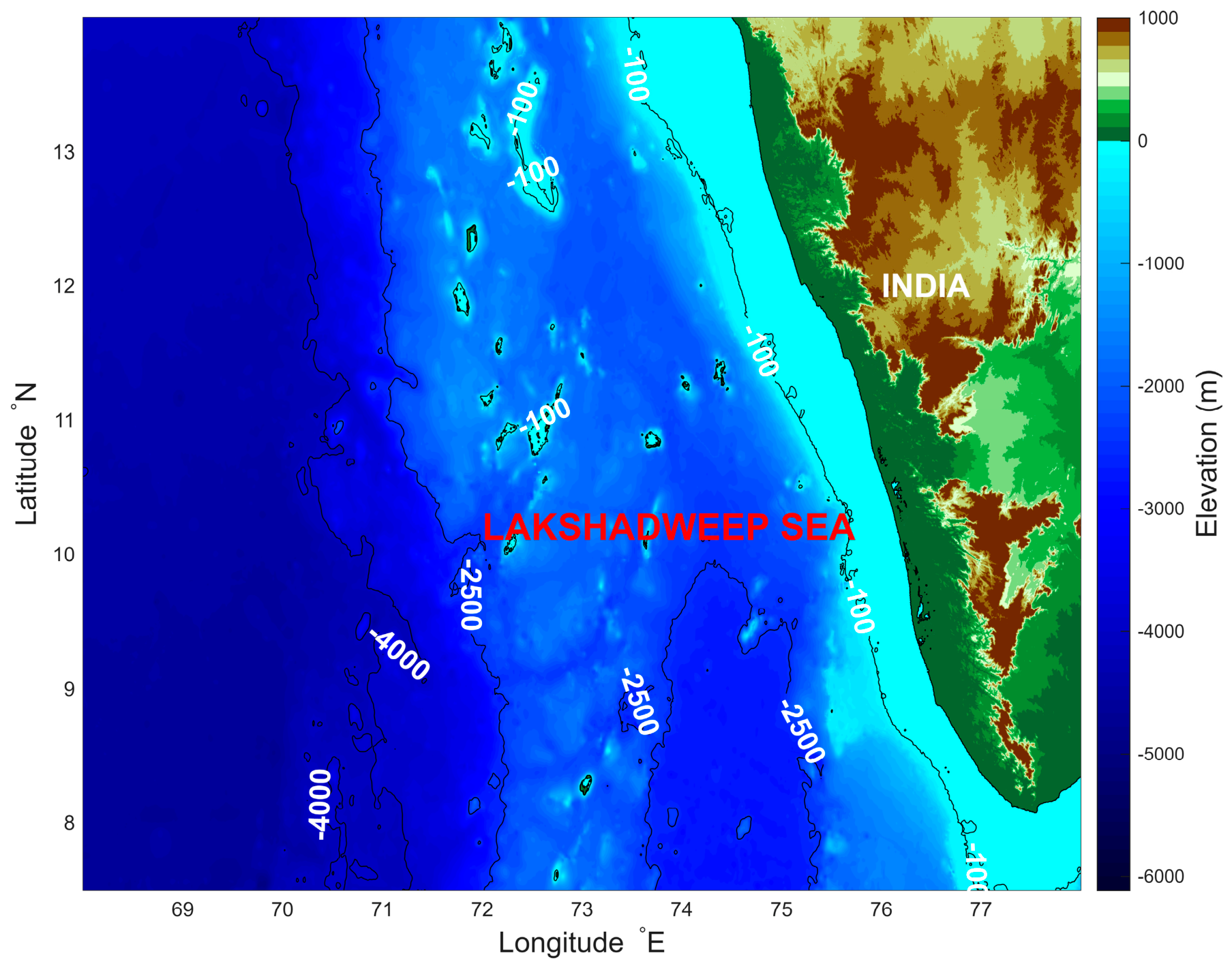
The Lakshadweep Sea is located in the southeastern Arabian Sea between the southwest coast of India, the Maldives, and Sri Lanka; see Figure 1.

It is one of the most productive marine regions in the northern Indian Ocean. The area supports diverse coral reef ecosystems, commercially important fisheries, and a wide range of marine organisms. Crucially, the Lakshadweep Sea supports the livelihoods of a significant proportion of the local population; see, e.g., [1,2]. The abundance and distribution of marine ecosystems are strongly influenced by seasonal oceanographic processes. Among these processes, coastal upwelling during the southwest monsoon plays a particularly important role in regulating biological productivity and ecosystem dynamics. Upwelling brings cold, nutrient-rich subsurface waters into the euphotic zone, stimulating phytoplankton growth and enhancing primary production. The resulting increase in biological productivity propagates into higher trophic levels and supports coastal fisheries [3,4].

Previous studies have shown that variations in upwelling intensity affect phytoplankton biomass, community structure, fish abundance, and regional carbon cycling [5]. Recent studies have further demonstrated that upwelled waters substantially affect the partial pressure of carbon dioxide (pCO₂) in the surface ocean. Although upwelling initially increases dissolved CO₂ concentrations by advecting carbon-rich subsurface waters towards the surface, subsequent biological uptake during phytoplankton blooms can partially offset these increases through photosynthetic carbon fixation. Accurate characterisation of upwelling variability is therefore essential for understanding ecosystem dynamics and air–sea carbon exchange in the Southeast Arabian Sea [6]. A multidisciplinary study of the physical and biological parameters of the Lakshadweep Sea upwelling carried out from 29 April to 7 November 2018 confirmed that physical factors strongly affect the abundance and structure of the phytoplankton community [7].

The upwelling system of the southeastern Arabian Sea is governed by a combination of local and remote physical processes. Alongshore winds associated with the southwest monsoon generate offshore Ekman transport, while positive wind-stress curl contributes through Ekman pumping. In addition, remotely forced Kelvin and Rossby waves, large-scale circulation patterns, remote winds in the Bay of Bengal and the equatorial Indian Ocean, and mesoscale eddies influence the timing, intensity, and spatial extent of upwelling [8,9].

The strength and spatial extent of upwelling in the Lakshadweep Sea vary from year to year in response to oceanic and atmospheric climate variability, including variations in the Indian Ocean Dipole [10] and properties of the southwest monsoon. Quantifying these variations requires robust indicators of upwelling intensity that adequately represent the underlying physical processes. Such indicators should ideally be capable of capturing the integrated response of coastal upwelling to multiple forcing mechanisms while remaining relatively insensitive to observational limitations.

To address the need for quantitative indicators of coastal upwelling intensity and its long-term variability, a variety of upwelling indices have been developed, primarily based on either wind data or satellite-derived sea surface temperature (SST). These indices condense different aspects of the upwelling process into a single quantitative metric, facilitating the analysis of historical variability and its links to marine ecosystem dynamics and fisheries. Among these, the Bakun upwelling index, introduced in 1973, remains one of the most widely used because of its conceptual simplicity and the availability of long-term wind records [11,12]. The index uses alongshore wind stress to estimate offshore Ekman transport, which serves as a proxy for the intensity of coastal upwelling.

Although the Bakun index provides a useful first-order estimate of wind-driven coastal divergence, it does not account for several processes that influence coastal upwelling because of the simplifying assumptions underlying Ekman transport theory. These processes include remote forcing, geostrophic transport, mesoscale variability, and wind-stress-curl-induced upwelling [8,9,13]. Coastal upwelling driven by Ekman transport and that generated by wind stress curl frequently coexist and overlap spatially, making their individual contributions difficult to distinguish [14,15,16]. Moreover, the reduction in wind speed towards the coastline (the coastal wind drop-off) enhances the cross-shore wind stress gradient and strengthens wind-stress-curl-induced upwelling, further increasing the overlap between the two mechanisms [17]. Consequently, wind-only indices such as the Bakun index cannot fully capture the spatial and temporal complexity of coastal upwelling and may provide an incomplete representation of its intensity.

To overcome some of these limitations, sea surface temperature (SST)-based upwelling indices have been developed to quantify the oceanic response directly. These indices typically estimate upwelling intensity from the thermal contrast between the cooler coastal waters affected by upwelling and the warmer offshore waters at the same latitude, thereby providing a measure of the surface manifestation of upwelling [18,19]. Satellite SST observations provide valuable information on the surface signature of upwelling, but their application in the Arabian Sea is complicated by extensive cloud cover and heavy precipitation during the southwest monsoon. These factors result in a cold bias and necessitate significant interpolation in Level 4 infrared data streams [20,21]. Microwave radiometers can partially overcome cloud contamination; however, their accuracy is substantially reduced by atmospheric water vapour and, in particular, heavy precipitation [22,23,24]. Consequently, the quality of satellite SST observations vary between years, complicating the interpretation of interannual changes in upwelling intensity. Furthermore, coastal cooling may result from the horizontal advection of colder surface waters from the north or the Bay of Bengal rather than from vertical transport, making SST an imperfect proxy for upwelling intensity [8,19].

Sea surface temperature (SST) observations derived from satellite imagery also have limitations in representing the biological response to coastal upwelling. During the pre-upwelling and early upwelling phases, the oligotrophic coastal waters of the southeastern Arabian Sea are highly transparent, with euphotic depths frequently exceeding 30 m [25,26]. As a result, nutrient-rich waters entering the lower and middle euphotic zone may stimulate primary production well before a noticeable cooling signal appears at the sea surface. Surface-only based indicators may therefore underestimate both the onset and the intensity of biologically significant upwelling events. Furthermore, the highly variable spatial extent and temporal evolution of coastal upwelling make it difficult to characterise its overall strength using instantaneous SST patterns alone [19].

Recent developments have led to the introduction of more comprehensive upwelling metrics, such as the Coastal Upwelling Transport Index (CUTI), which combines Ekman transport with geostrophic cross-shore transport to provide a more complete representation of coastal upwelling [13,27]. Although these approaches represent an important advance over wind-only based indices, they do not explicitly account for remote forcing associated with coastally trapped Kelvin waves, Rossby waves, or other basin-/regional-scale oceanic processes, and therefore remain subject to additional assumptions and uncertainties [13]. Direct hydrographic observations have also been used to quantify coastal upwelling. For example, in the Black Sea, upwelling intensity has been estimated from the temperature difference between fixed stations located within the coastal upwelling zone and offshore waters [28]. While observational approaches provide a more direct measure of the oceanic response, their spatial and temporal coverage is generally limited, restricting their applicability for long-term and large-scale assessments.

These limitations motivate the development of alternative indices that quantify the oceanic response directly rather than relying solely on atmospheric forcing. To represent the three-dimensional (3D) thermal structure of the coastal ocean, we employ a modern high-resolution data-assimilative ocean model. A key advantage of an ocean model is that it resolves the early subsurface development of upwelling, including stages that have no detectable surface expression. In the southeastern Arabian Sea, for example, shoreward shoaling of the isopycnals may begin well before cold water becomes visible at the sea surface [29,30]. Consequently, the initiation and evolution of upwelling can be identified well before SST-based indices respond.

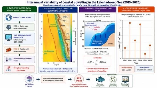
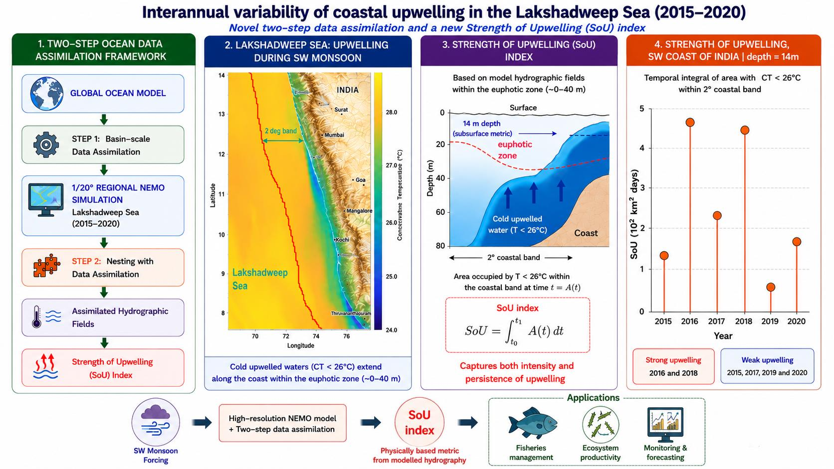
Using the model’s three-dimensional temperature fields, we introduce a new Strength of Upwelling (SoU) index that quantifies coastal upwelling directly from the thermal structure of the coastal ocean. Unlike existing wind-based indices, which infer upwelling intensity from atmospheric forcing, or SST-based indices, which rely on the surface thermal expression of upwelling, the SoU index is calculated as the temporal integral of the Cold Water Area (CA), defined as the area occupied by waters colder than a specified temperature threshold within the euphotic layer. The index therefore integrates information on both the spatial extent and temporal persistence of cold upwelled water into a single quantitative metric, allowing the overall intensity of an upwelling season to be characterised by a single parameter.

To demonstrate the proposed approach, we apply the SoU index to 3D temperature fields produced by a high-resolution regional ocean model for the Lakshadweep Sea. This enables us to quantify the seasonal, spatial, and interannual variability of coastal upwelling and to investigate its relationship with large-scale climatic variability. The proposed methodology provides a general framework for quantifying coastal upwelling from high-resolution 3D ocean model outputs and is readily transferable to other coastal upwelling systems.

2. Materials and Methods

2.1. Model Configuration

This study uses outputs from a high-resolution regional ocean model of the Lakshadweep Sea (hereafter referred to as LD20) covering the domain 7.5–14.5° N and 68–78° E for the period 1 January 2015–31 December 2020. A brief description of the model is provided below; full details are available in [31]. The model is based on version 3.6 of the Nucleus for European Modelling of the Ocean (NEMO) modelling engine [32] and is implemented within the ROSE-CYLC workflow environment, which is used to configure, manage, and run highly complex computer models [33]. The model has a horizontal resolution of 1/20° × 1/20° and 50 vertical levels.

LD20 is nested within the Copernicus Marine Environment Monitoring Service (CMEMS) global ocean reanalysis product GLOBAL_REANALYSIS_PHY_001_030 (hereafter CMEMS_12), which has a horizontal resolution of 1/12° [34]. The LD20 model uses the same geopotential computational levels as the parent CMEMS_12 model, and those are fixed throughout the domain. The depth levels used for the analysis are the actual computational “grid_T” levels without any vertical interpolation. The LD20 model employs a two-step data assimilation technology referred to as Nesting with Data Assimilation (NDA) [31,35,36,37]. Atmospheric forcing is provided by the UK Met Office Unified Model, with product NWP768 used from 1 January 2015 to 31 August 2017 and product NWP1280 thereafter. Atmospheric variables were supplied at 3-hourly intervals, except for surface winds, which were available hourly [38].

Initial and lateral boundary conditions for temperature, salinity, and horizontal velocity were obtained from CMEMS_12. Tidal forcing was introduced through nine harmonic constituents (M2, S2, N2, K2, K1, O1, P1, Q1, and M4) derived from the TPXO 7.2 global tidal solution [39]. These tidal velocities were superimposed on the non-tidal barotropic velocities obtained from CMEMS_12. Bathymetry was sub-sampled from the GEBCO-2014 gridded bathymetric dataset [40].

Horizontal viscosity was parameterised using the Laplacian form of the Smagorinsky scheme. Horizontal tracer diffusion was represented by a combination of Laplacian and biharmonic operators, with coefficients identical to those used by [34]. Vertical turbulent mixing was parameterized using the k–ε implementation of the General Length Scale (GLS) turbulence closure scheme. The baroclinic and barotropic time steps were 120 s and 6 s, respectively.

2.2. Nesting with Data Assimilation

The LD20 model employs a two-step Nesting with Data Assimilation (NDA) framework, which combines information from a data-assimilative global ocean reanalysis with a regional ocean model, thereby improving the realism of the simulated hydrographic fields [34,38]. NDA consists of two sequential steps. The first step involves the assimilation of observations into a coarse resolution parent model, CMEMS_12, using the NEMOVAR 3D variational data assimilation system. This step is performed operationally within the CMEMS_12 production framework [33] and produces dynamically consistent 3D fields of temperature, salinity, and velocity, as well as a two-dimensional field of sea level. In the second step, the multivariate 3D state estimates from the parent CMEMS_12 model are assimilated into the child model, thereby linking the regional LD20 model with real-world observations.

Assimilation of parent-model fields offers several advantages. The assimilated variables are available on regular spatial and temporal grids, and observational information has already been propagated into data-sparse regions through the laws of fluid dynamics and the parent assimilation system. This approach avoids many of the practical difficulties associated with the direct assimilation of sparse observations into a high-resolution model. For example, maintaining dynamical consistency between density and velocity in ocean data assimilation is a fundamental requirement to prevent unphysical shocks, such as the generation of spurious internal waves, following the assimilation of observations into numerical models; see, e.g., [41]. As the velocity and density fields inherited from the parent model are already dynamically balanced, no additional balancing procedures are required. Another advantage of the NDA methodology is that it reduces the so-called “double penalty effect” [34,42].

A key distinction between NDA and conventional data assimilation approaches lies in the treatment of error covariance matrices. Because the assimilated quantities (pseudo-observations) originate from a numerical model rather than from independent observations, their errors cannot be assumed to be spatially uncorrelated. Therefore, the observation error covariance matrix is non-diagonal and must be estimated explicitly. The methodology for estimating the background and observation error covariance matrices together with other aspects of model-to-model assimilation is described in detail in [42]. The NDA method is computationally efficient, making it well suited to computationally demanding applications, including ensemble modelling and high-resolution regional forecasting. The accuracy of the LD20 model and the improvements achieved through the NDA technique have been assessed in detail in [34,35] and are therefore not repeated here.

2.3. Stochastic–Deterministic Downscaling

The second step of the NDA process consists of two components. The first component is purely data-driven. It involves a transfer of information from the coarse-resolution parent model to the higher-resolution regional grid using stochastic properties of model outputs. The stochastic component is based on the concept of objective analysis; it represents the Best Linear Unbiased Estimator (BLUE), and is capable of recovering finer-scale features which are only embryonically resolved by the parent model [43]. The second component combines the running of a dynamic ocean model (in this case LD20) and assimilation of the downscaled 3D fields from the parent CMEMS_12 model data into the LD20 model. The second component includes temporal interpolation of the parent model fields and calculation and application of Kalman filter gain weights at each assimilation cycle. In the case of LD20, the DA cycle is five days and assimilation occurs at 00:00 GMT.

Model performance was evaluated against multiple independent datasets, including OSTIA (Operational Sea Surface Temperature and Sea Ice Analysis), ARGO temperature and salinity profiles, GHRSST-MUR (Group for High Resolution Sea Surface Temperature-Multiscale Ultrahigh Resolution) Level 4 dataset, and observations from local weather buoys; see [34,42] for details of model validation. It was also verified against the data assimilating Copernicus global model GLOBAL_REANALYSIS_PHY_001_030-TDS. To further assess the model performance within the study region, Figure 2 compares the area-averaged SST from LD20 and OSTIA over the six-year study period within a coastal band extending 2° offshore between 8.2° N and 14.2° N. This coastal band was selected to isolate the upwelling region because the full LD20 domain extends as far as 700 km offshore, where the ocean circulation is dominated by different dynamical processes.

The SST obtained from the LD20 model is generally consistent with OSTIA. The only noticeable discrepancy occurs in 2015, where OSTIA shows colder surface waters than the model. The difference is likely caused by the inflow of cold surface waters from the Bay of Bengal through a very narrow and shallow Palk Strait between Sri Lanka and India near the eastern boundary of the model domain, which was not captured by the CMEMS_12 model.

3. Results

3.1. Pre-Monsoon Conditions

The LD20 simulations cover the period from 1 January 2015 to 31 December 2020 and provide a detailed representation of the seasonal and interannual evolution of upwelling in the Lakshadweep Sea. The upwelling lifecycle is commonly divided into four stages: pre-monsoon (or inter-monsoon) stage followed by the onset, peak, and decay stages [3,4,7,8]. Before examining the interannual variability of upwelling during the southwest monsoon, it is useful to consider the initial hydrographic conditions preceding its onset.

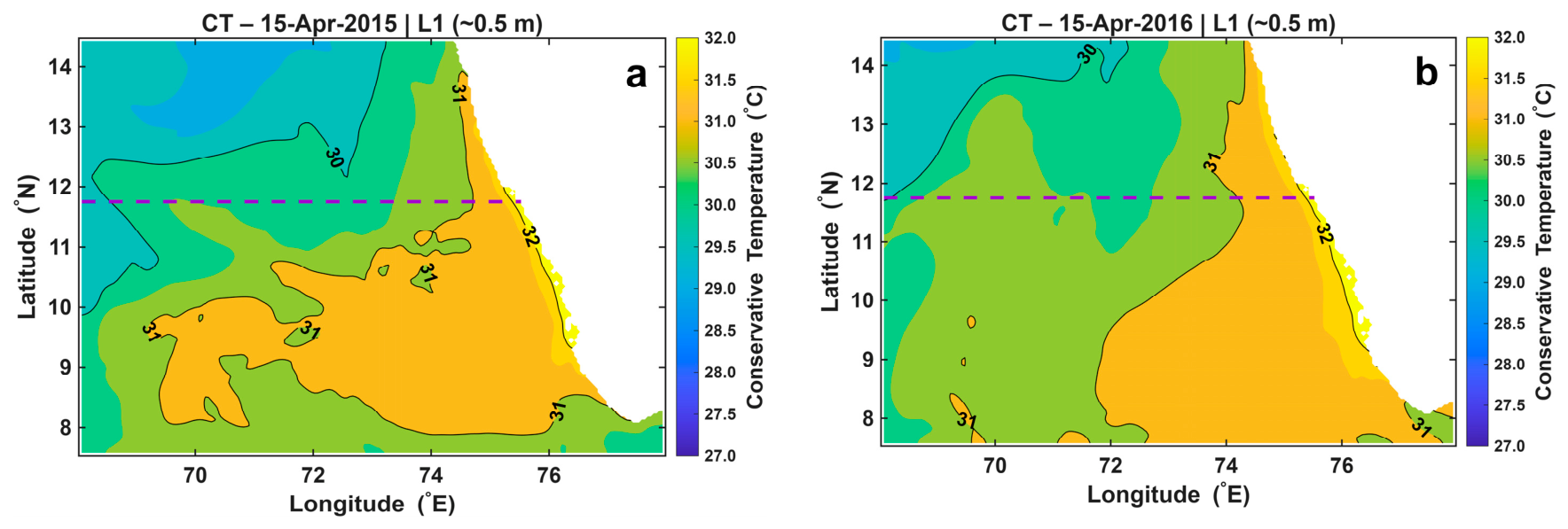
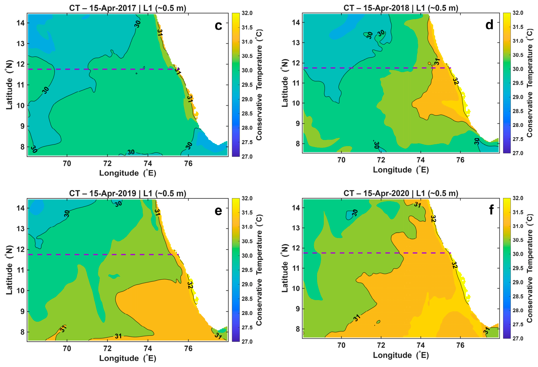
The northeast monsoon typically persists until March, followed by an inter-monsoon period during April and May before the onset of the southwest monsoon. Sea surface temperature (SST) distributions on 15 April, representing the middle of the inter-monsoon period of each study year, are shown in Figure 3. The SST patterns during this period are generally similar among years, with relatively warm (31–32 °C) surface waters occupying most of the study area. Slightly lower SSTs are evident in 2017 and 2018, whereas conditions in 2015, 2016, 2019, and 2020 are broadly comparable.

Subsurface conditions exhibit somewhat different characteristics. Temperatures at approximately 27 m depth, near the lower boundary of the euphotic layer, were lower in 2019 than in the other study years both in the open ocean and within the coastal strip. In addition, a large cold spot was present in the southern coastal sector during 2017. In contrast to surface temperature, the subsurface isopycnals show little evidence of preconditioning for coastal upwelling in mid-April for all years of study. The density structure is controlled primarily by temperature; therefore, salinity variations play a minor role.

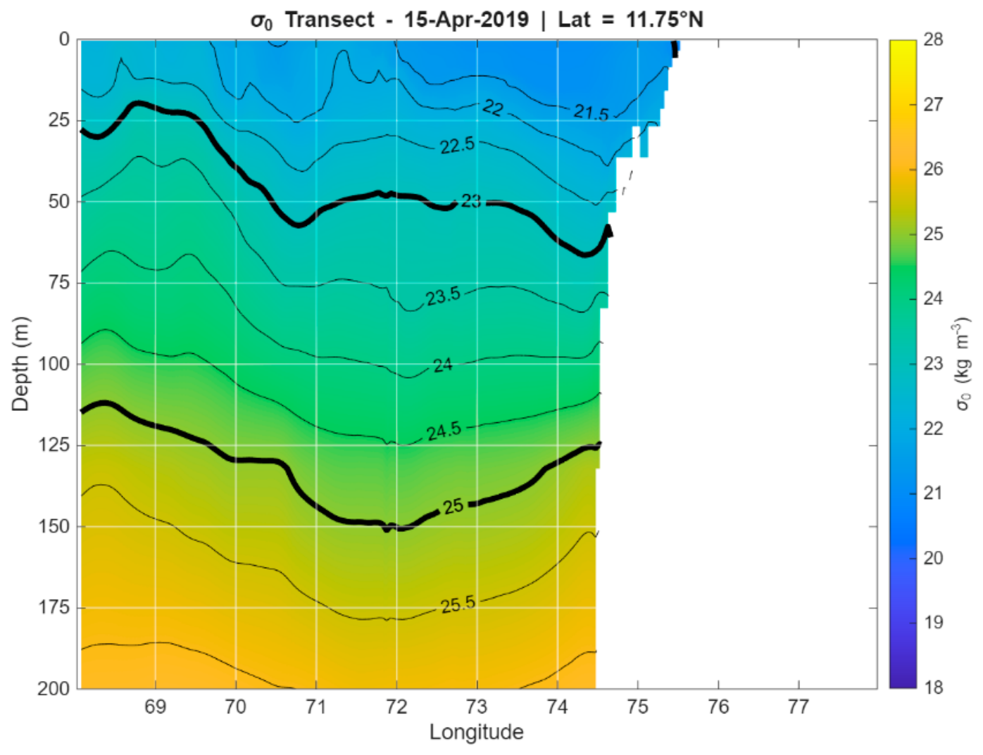
An example of the pre-monsoon density structure is presented in Figure 4, which shows a potential density transect along 11.75° N (slightly north of Kochi, the commercial capital of the state of Kerala) on 15 April 2019. The isopycnals are largely horizontal with no significant shoaling of density surfaces towards the coast, indicating that the upwelling circulation had not yet become established during the inter-monsoon period. The transects from other study years exhibit little interannual variability.

This result is consistent with field observations reported in [7], which showed no evidence of significant shoaling of the 26 °C isotherm during the pre-upwelling phase in 2018.

3.2. Onset of Upwelling

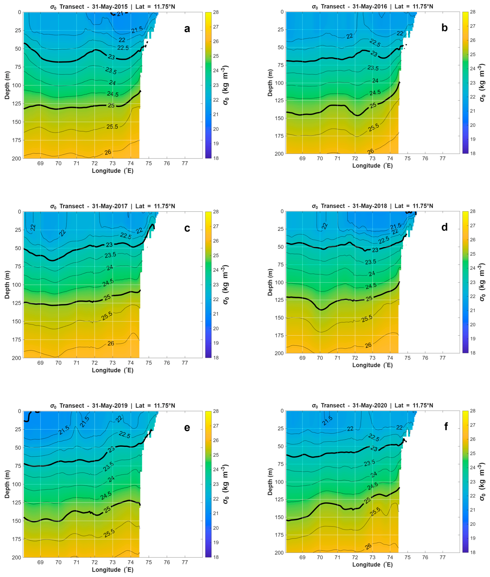
By the end of May, the hydrographic structure changes markedly. Figure 5 presents potential density transects along 11.75° N on 31 May for all six study years. Compared with the April conditions, the density field exhibits clear evidence of the upward displacement of subsurface waters in the coastal zone.

For example, the σ₀ = 23.0 kg m⁻³ isopycnal, which is typically located between 50 and 75 m depth offshore, shoals towards the coast and approaches the base of the euphotic layer. This shoreward shoaling marks the onset of coastal upwelling and indicates the upward transport of nutrient-rich subsurface waters into the biologically active layer. As during the inter-monsoon season, the interannual differences remain relatively small at this early stage of upwelling.

Figure 5. Potential density transects at 11.75° N on the 31st May for the six years of study (a–f). The shoreward shoaling marks the onset of coastal upwelling. The differences in the density structure between the years are minimal.

Figure 5. Potential density transects at 11.75° N on the 31st May for the six years of study (a–f). The shoreward shoaling marks the onset of coastal upwelling. The differences in the density structure between the years are minimal.

3.3. Peak of Upwelling

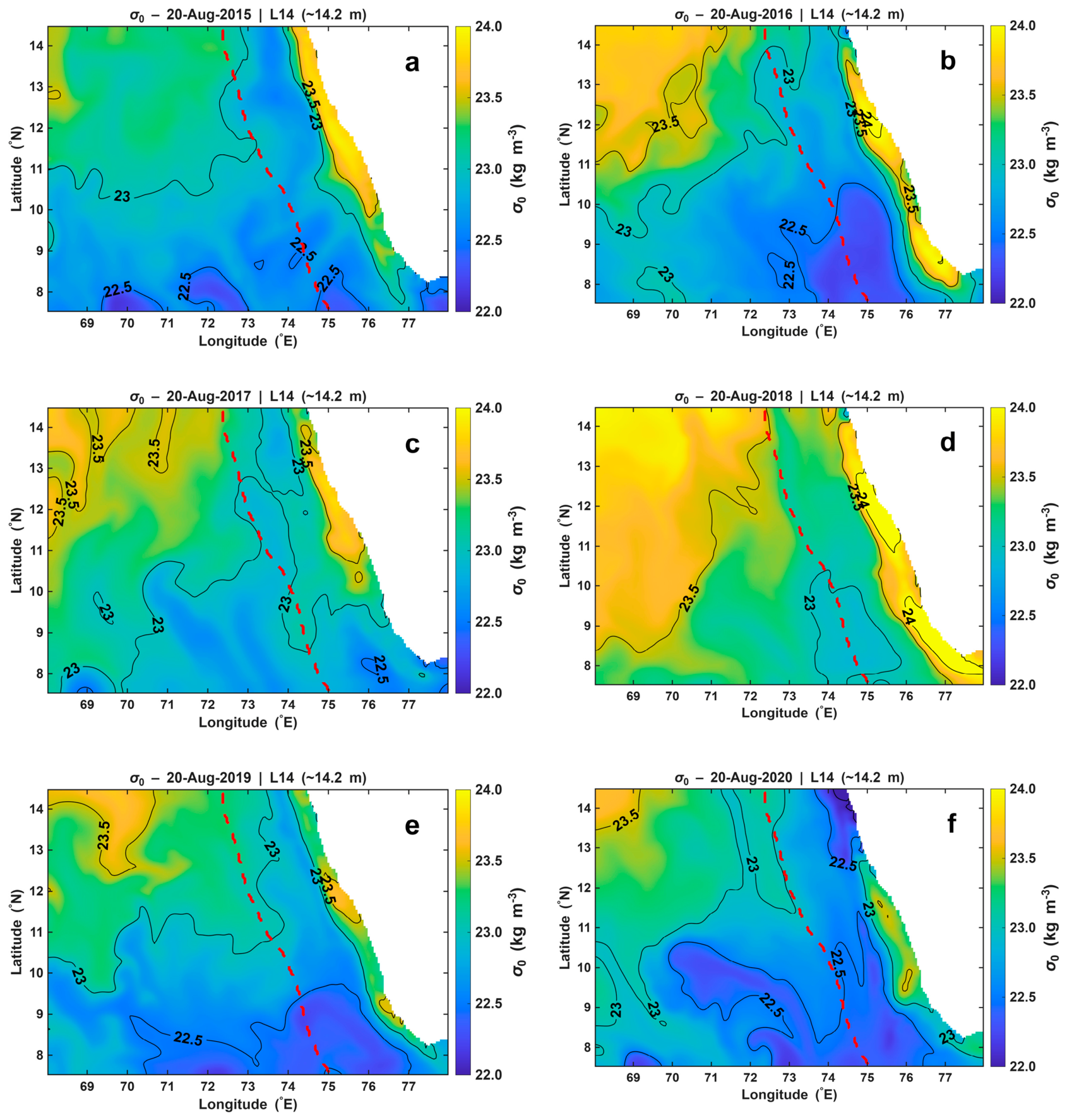
Interannual differences become substantially more pronounced during the mature phase of the upwelling season. Figure 6 shows potential density distributions on 20 August at 14.2 m depth corresponding approximately to the middle of the euphotic layer. This depth was selected to minimise the influence of transient surface warming while retaining the hydrographic signature of upwelled waters.

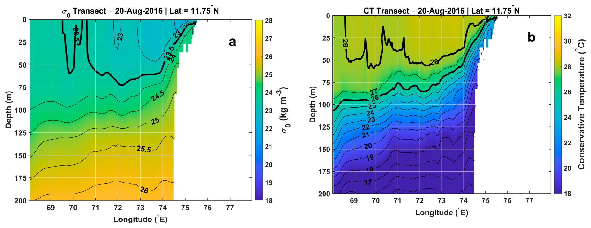
Two distinct regions of elevated density (σ₀ > 23.0 kg m⁻³) are apparent. The first occupies the northwestern part of the model domain and is associated with the equatorward transport of relatively cold waters by the West India Coastal Current [3,8]. The second forms a narrow coastal band extending along the southwest coast of India and represents the direct hydrographic signature of coastal upwelling. The distinction between these two features is illustrated in Figure 7, which presents potential density and conservative temperature transects along 11.75° N on 20 August 2016, which was the year of strong upwelling—see below. The transects clearly show the upward displacement of cold, dense waters towards the coast and the deep ocean dense-water patch further offshore.

The upward displacement of cold, dense waters towards the coast during the peak season produced by the LD20 model is similar to that observed in [7] between 5 and 22 August 2018; see their Figure 2.

3.4. Variability of Cold Water Area

To characterise the spatial and temporal evolution of coastal upwelling and facilitate the analysis of its interannual variability, we introduce the Cold Water Area (CA), defined as the area occupied by waters colder than a prescribed temperature threshold within a coastal band. Because the Cold Water Area is calculated directly from the 3D distribution of the temperature field rather than from atmospheric forcing proxies such as wind stress, it provides a more direct measure of upwelling. The CA provides the basis for the Strength of Upwelling (SoU) index, which is introduced in the following section.

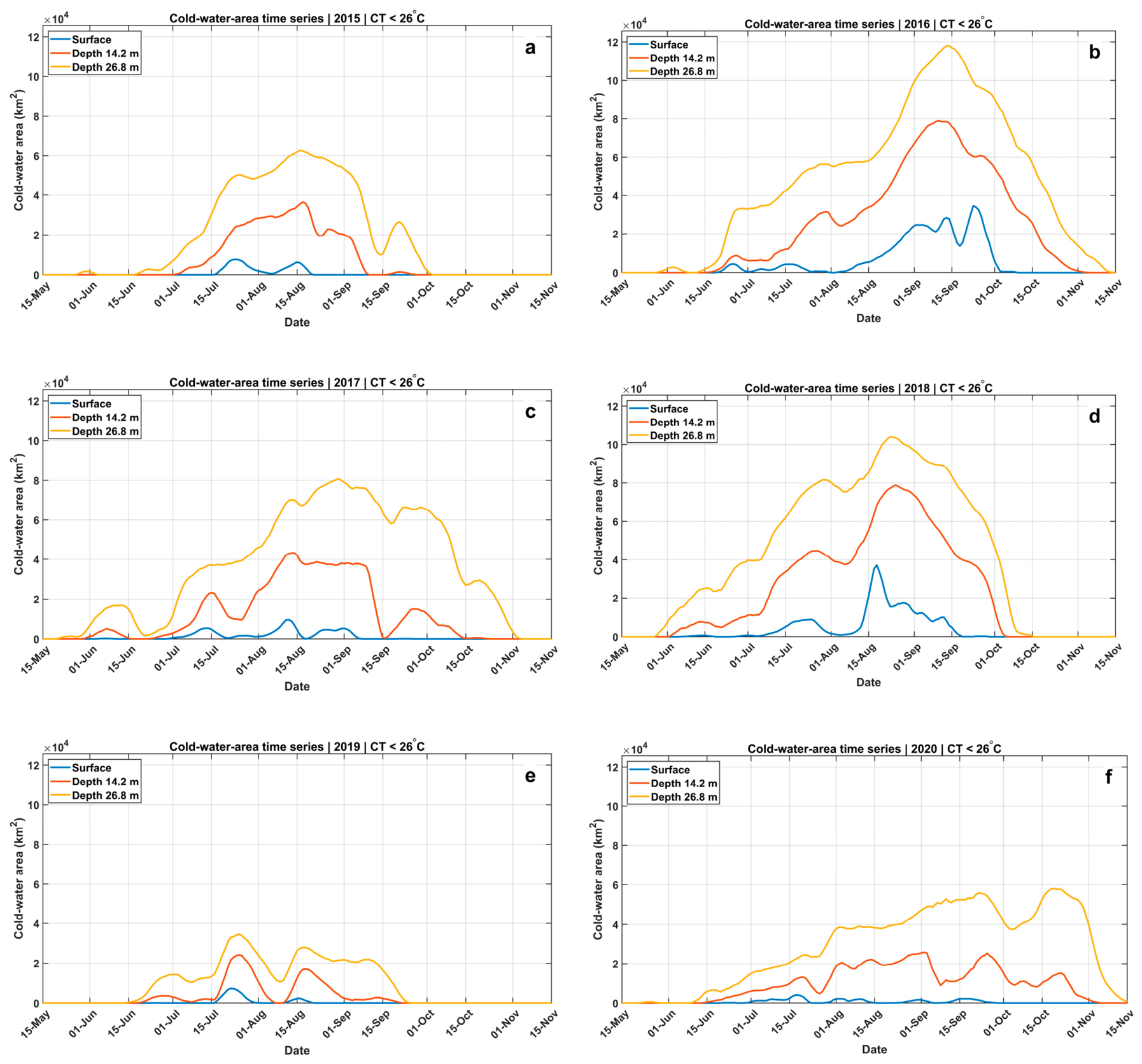
Consistent with previous studies of the Lakshadweep upwelling system [3,8], a threshold temperature of 26 °C is adopted, and the CA is calculated within a coastal band extending 2° offshore from the coastline. Restricting the analysis to the 2° coastal band avoids contamination by cold-water features in the open ocean that are unrelated to coastal upwelling. The sensitivity test has been carried out to show that the assessment of the interannual variability of upwelling is insensitive to the threshold temperature in the range of 25.5 to 27 °C. The CA is calculated daily throughout the southwest monsoon season (15 May–15 November) at multiple depth levels between the surface and 53 m and then smoothed with a 5-day window for clarity of presentation (Figure 8). The coastal area strip of dense and cold water has different extension, shape, minimum temperature, and maximum density in different years and different stages of the upwelling season; see, e.g., Figure 6 and Figure 8.

There is a considerable interannual variation in the characteristics of coastal upwelling. The most pronounced upwelling occurred in 2016 and 2018, when the upwelled waters were both denser and colder and occupied a substantially larger area than in 2015, 2017, 2019, and 2020. This contrasts with the pre-monsoon state when colder waters were present in 2017 but not in 2016. By contrast, 2018 exhibited a greater consistency between the pre-monsoon and early monsoon conditions, with lower temperatures evident during both periods. The spatial structure of upwelling also differs between years. In 2018, two distinct density maxima were present near 8.5° N and 12° N, whereas in 2020 the dense-water signal was weaker and more diffuse, extending broadly between 9° N and 12° N. These results indicate that the intensity of mature upwelling cannot always be inferred from the hydrographic conditions during the pre-monsoon period.

The temporal evolution of Cold Water Area reflects both the development and persistence of upwelled waters throughout the southwest monsoon season. Although all depth levels reveal the inter-monthly and interannual signal, the largest contrasts occurred at 14 m depth. The maximum area occupied by waters colder than 26 °C at this depth during peak upwelling nearly doubled between 2015 and 2016, increasing from approximately $0.63\times {10}^5$ km² to $1.2\times {10}^5$ km². This depth lies near the middle of the euphotic zone and therefore captures hydrographic changes that are likely to be most relevant to biological productivity. At the surface, the upwelling signal may be partially obscured by atmospheric heating and wind/wave mixing, whereas subsurface layers more directly reflect the upward displacement of thermocline waters.

3.5. Strength of Upwelling Index

To characterise the cumulative effect of upwelling over the southwest monsoon season, the Strength of Upwelling (SoU) index is introduced as the temporal integral of the Cold Water Area time series at a given depth level. The SoU therefore combines both the spatial extent and duration of upwelling into a single metric. Graphically, the SoU corresponds to the area under curves shown in Figure 8, and it is a measure of heat content within the upwelling area at a specific depth level. The concept underlying the SoU index is similar to the Growing Degree Days index used in agriculture, ecology and phenology to quantify cumulative thermal conditions controlling plant development; see, e.g., [44,45].

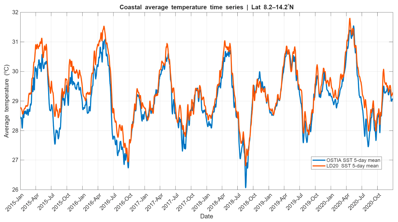
The accuracy of both CA and SoU is dependent on the uncertainty of the underlying numerical model. It is therefore crucial to utilise a modern model incorporating an efficient data assimilation technique. As integral metrics, the CA and SoU benefit from a model with minimal bias against observations. The LD20 model exhibits a minor bias of 0.23 °C against OSTIA and −0.08 °C to 0.22 °C against coastal weather buoys [31], making its output suitable for calculating these new upwelling metrics. Furthermore, analysing interannual variability requires maintaining an identical model configuration across the entire study period to ensure bias consistency.

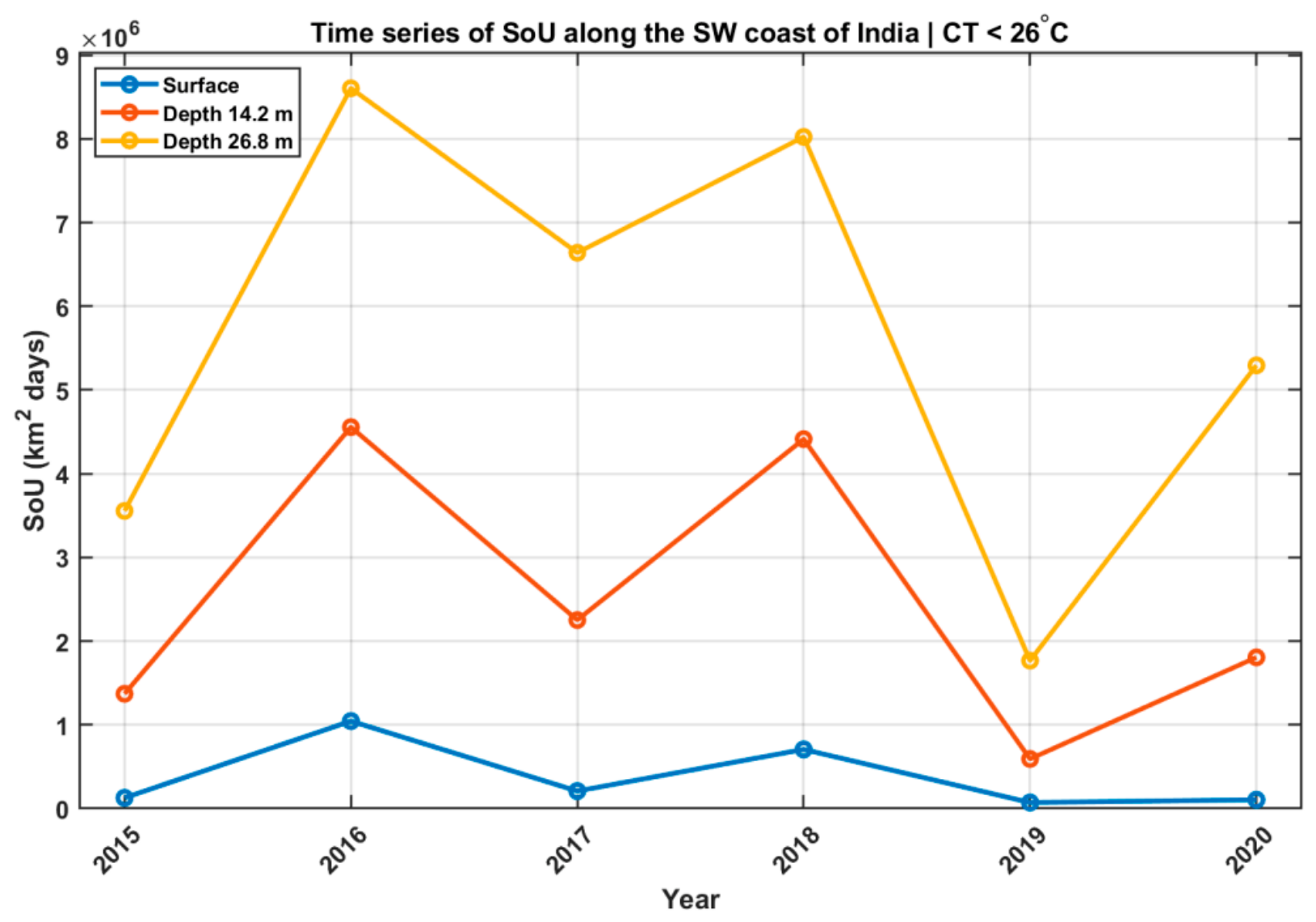
Figure 9 presents SoU values calculated at several depth levels. The index clearly distinguishes years of strong and weak upwelling at all three depth levels. The highest values occurred in 2016 and 2018, whereas 2015, 2017, and 2019 were characterised by substantially weaker upwelling. The year 2020 represents an intermediate case in which the surface expression of upwelling was weak, but a subsurface signal remained evident at greater depths. Comparison between depth levels highlights an important aspect of the upwelling system: in some years, particularly 2020, the upwelling signature is considerably stronger below the surface than at the surface itself. This result suggests that assessments based solely on SST may underestimate the intensity of upwelling when near-surface warming masks the subsurface intrusion of cold waters.

3.6. Latitudinal Variability

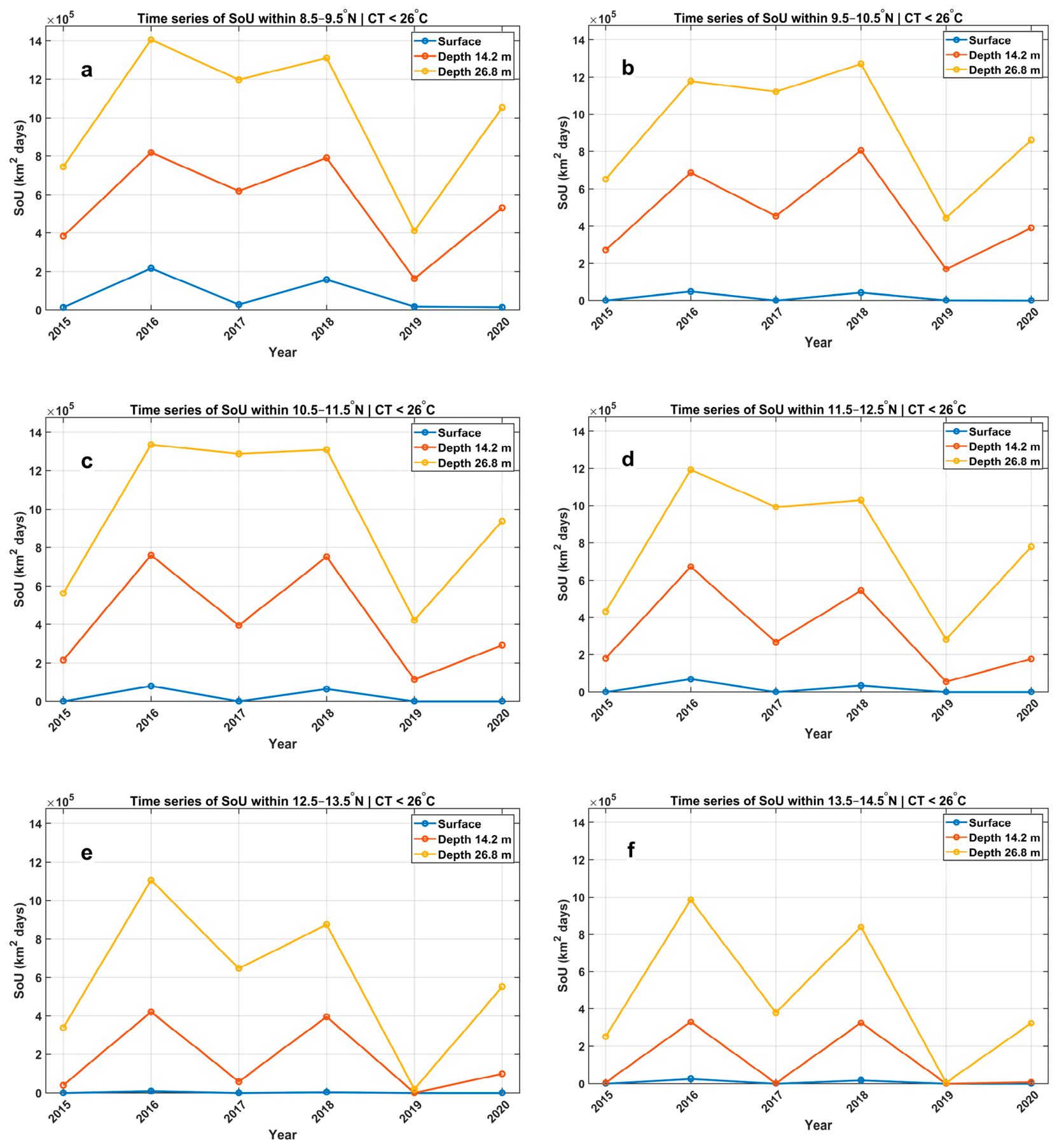
For practical applications, it is helpful to assess the strength of upwelling at different locations along the Indian coast as coastal fisheries are often influenced by local oceanographic conditions. This is particularly relevant for small-scale fisheries, where fishing activities are typically confined to relatively limited areas. The SoU index was calculated for adjacent 2° latitude bands along the southwest coast of India in order to examine spatial variability in upwelling intensity; see Figure 10. Considerable latitudinal variations are evident, with different coastal sectors exhibiting distinct interannual variability.

Both the CA time series and the more compact SoU index identify 2016 and 2018 as years of enhanced upwelling and 2015, 2017, 2019, and 2020 as years of comparatively weak upwelling. Although the strongest upwelling generally occurred in 2016 and 2018 throughout the region, the relative magnitude of the SoU varied among latitude bands. For example, SoU values in 2016 and 2018 are nearly identical within the 8.5–9.5° N, 10.5–11.5° N, 12.5–13.5° N and 13.5–14.5° N bands, whereas 2018 exhibits stronger upwelling than 2016 within 9.5–10.5° N and weaker upwelling within 11.5–12.5° N.

The relationship between upwelling variability and the Indian Ocean Dipole (IOD) is of particular interest and has been extensively studied [10,46]. The Dipole Mode Index (DMI), which measures the zonal sea surface temperature gradient across the tropical Indian Ocean [47], is widely used to characterise basin-scale climate variability. Variations in the DMI are reflected, to some extent, in variations in the SoU index. For example, the strong negative IOD event of 2016 was associated with enhanced SoU values throughout much of the study area. Conversely, the positive DMI of 2019 corresponded to weaker upwelling and a reduced extent of cold water intrusion (Figure 8 and Figure 9). The DMI values in June 2018 were comparable to, or slightly more positive than, those during June 2017 [47], yet the SoU index indicates substantially stronger upwelling in 2018. Similar differences are observed across individual latitudinal bands. Thus, the SoU variations are broadly consistent with previous studies [10,46] linking upwelling intensity in the southeastern Arabian Sea to variations in the IOD. However, our results show that the SoU responds to the basin-scale climate signal but is not fully controlled by it.

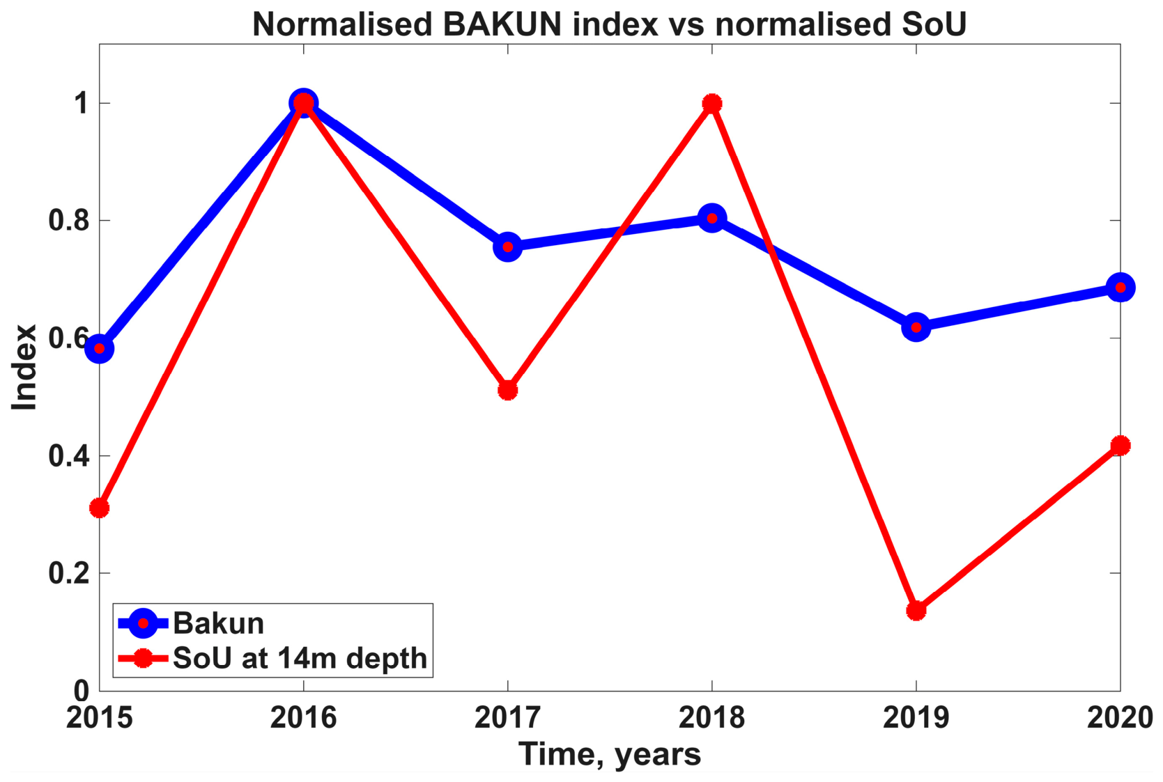
A comparison of interannual variability represented by the Bakun and SoU indices is illustrated in Figure 11. Both indices are calculated for the same 2° coastal band over the same monsoon period. Although both indices characterise the intensity of upwelling, they quantify different aspects of the process. The Bakun index estimates wind-driven offshore Ekman transport as a proxy for upwelling intensity. In contrast, the SoU index is derived from the area occupied by cold upwelled water in the euphotic zone (or, when required, at the sea surface), thereby representing the thermal structure of the coastal ocean. Because the two indices have different physical meanings and units, they are compared using normalised values obtained by dividing each index by its maximum value over the study period. The comparison is intended to assess the extent to which variability in atmospheric forcing is reflected in the oceanic response.

Both Bakun and SoU indices identify the same years of strong and weak upwelling; however, they differ in the magnitude of the upwelling signal. In 2018, the Bakun index suggests a weaker upwelling signal than the SoU index, whereas in 2015, 2017, 2019, and 2020 it indicates a relatively stronger signal. The close agreement in the interannual ranking shown in Figure 11 indicates that wind-driven Ekman transport is the dominant control on upwelling variability in the study region. The remaining differences are likely to reflect the influence of physical processes that are not represented by the Bakun index, including remote forcing, geostrophic transport, and wind-stress-curl-induced upwelling.

This interpretation is consistent with the findings of [48], who showed that incorporating both Ekman transport and Ekman pumping into a single metric improved the representation of the Arabian Sea upwelling. However, unlike the SoU index, their combined index remains entirely wind-based and therefore still represents the atmospheric forcing rather than the oceanic response.

4. Discussion

The Lakshadweep Sea is among the most productive regions of the northern Indian Ocean [7,49], where the primary production is largely controlled by the supply of nutrients to the euphotic zone through vertical exchange processes (see, e.g., [50]). Quantifying the intensity and variability of this upwelling is therefore essential for understanding the functioning of the regional marine ecosystem [5].

Existing wind- and SST-based upwelling indices [11,12,18,19] have well-recognised limitations [8,9,13,14,15,16,17,21,22,23,24]. Wind-based indices rely on the simplifying assumptions of Ekman transport theory, whereas satellite SST observations are affected by persistent cloud cover, heavy precipitation, and other observational constraints during the southwest monsoon. Conversely, the proposed SoU index has a principal advantage in that it quantifies the oceanic response to the southwest monsoon directly from the 3D thermal structure of the water column. This study uses a high-resolution regional ocean model, LD20, employing a two-step data assimilation methodology for the accurate representation of the ocean state. The model is configured for the Lakshadweep Sea south of 14.5° N and is run for the period 2015–2020. The 3D model fields represent the full range of physical processes included in the numerical model, rather than just wind-driven Ekman transport.

To assess interannual variability, we introduce two complementary metrics. The first, the Cold Water Area (CA), quantifies the spatial extent of waters colder than 26 °C at a subsurface level within the biologically productive euphotic zone or, if required, at the surface. The threshold temperature and the depth of the euphotic zone are specific to the Lakshadweep Sea and require adjustment for other regions. The second metric, the Strength of Upwelling (SoU), integrates the CA time series over the southwest monsoon period and therefore captures both the intensity and persistence of upwelling. Together, the CA and SoU condense information contained in large 3D data sets into physically meaningful and simple-to-operate metrics. Applying the SoU index at subsurface depths reveals upwelling signals that may not be evident from sea surface temperature alone.

The analysis of 3D temperature fields and the SoU index demonstrates pronounced interannual variability in both the spatial extent and persistence of upwelled waters in the Lakshadweep Sea. Although this variability is broadly similar throughout the region, the magnitude of the SoU varies with latitude. These latitudinal differences indicate that local physical processes modulate the response of the coastal ocean to monsoon forcing, producing noticeable heterogeneity in upwelling intensity along the southwest Indian margin.

The properties of coastal waters along the southwest Indian coast are linked to large- scale atmospheric and oceanic processes. The Indian Ocean Dipole (IOD) represents large- scale climatic variations across the Indian Ocean and influences coastal upwelling in the region, shifting wind patterns and water temperatures between the eastern and western sides of the ocean [46]. The Indian Ocean Dipole is quantified by the DMI tracking the east–west temperature difference in the tropical Indian Ocean. However, local upwelling features and, therefore, the SoU index, do not strictly mirror basin-scale DMI variations. This divergence suggests that basin-scale, local, and regional processes act together to determine the hydrographic response of the coastal ocean to the monsoon forcing [10,49]. A comparison of the SoU with the wind-stress-only Bakun index helps to assess the contribution of wind stress relative to other physical processes influencing coastal upwelling. In agreement with previous research [48], this comparison indicates that Ekman transport is the dominant, though not exclusive, driver of upwelling intensity.

While this study focuses on a specific region of the ocean, the results suggest that the proposed Strength of Upwelling (SoU) index may serve as a practical tool for quantifying the temporal and spatial variability of coastal upwelling in other regions, subject to appropriate adjustment of the threshold temperature. By being derived from 3D hydrographic structures rather than atmospheric forcing alone, the SoU index complements existing wind-based tools by offering a physically meaningful metric for the oceanic response to monsoon forcing. Furthermore, the SoU index can be calculated for specific sub-sections of the coastal zone, serving as an integrated measure of local upwelling variability. As the SoU index is a newly introduced metric, these results represent the initial proof of concept. Further studies should evaluate its performance in other coastal upwelling systems.

5. Conclusions

This study investigates the interannual variability of coastal upwelling in the Lakshadweep Sea between 2015 and 2020, using a high-resolution (1/20°) NEMO-based regional ocean model (LD20) coupled with a two-step Nesting with Data Assimilation (NDA) framework. The model realistically reproduces the 3D thermal structure of the coastal ocean, enabling a detailed analysis of the seasonal evolution of upwelled waters within the euphotic zone.

A new metric, the Strength of Upwelling (SoU), was developed from daily model-derived temperature fields to quantify this variability. The SoU index is defined as the temporal integral of the spatial extent of waters colder than a region-specific threshold temperature (26 °C for the Lakshadweep Sea) at selected depth levels and therefore incorporates both the intensity and persistence of upwelling. In contrast to traditional wind-based indices, the SoU quantifies the oceanic conditions directly, accounting for the combined effects of all physical processes represented in the model.

The analysis identifies 2016 and 2018 as years of enhanced upwelling, characterised by a greater spatial extent and a more persistent intrusion of deep cold waters into the euphotic layer. Weaker upwelling occurred in 2015, 2017, 2019, and 2020. The largest interannual differences in the SoU were observed at 14 m depth, i.e., within the euphotic zone, suggesting that the subsurface thermal metric may provide a more robust characterisation of upwelling than surface-based indicators alone. Comparison with the Indian Ocean Dipole (IOD) index indicates that although large-scale climate variability contributes to the observed interannual differences, it does not fully explain them. Comparison with the wind-stress-based Bakun index confirms that Ekman transport is the dominant driver of upwelling while also indicating a substantial contribution from other physical processes.