


Abstract
Climate change poses escalating risks to environmental, economic, and social systems worldwide, making accurate temperature forecasting a critical component of climate impact assessment and mitigation planning. Advances in data-driven modelling have expanded the range of tools available for analysing climate time series, complementing traditional statistical approaches. The continued increase in global surface temperatures, driven primarily by anthropogenic greenhouse gas (GHG) emissions, underscores the need for forecasting models capable of capturing complex and non-linear climate dynamics. This study compares the predictive performance of a Long Short-Term Memory (LSTM) neural network with a Seasonal Autoregressive Integrated Moving Average (SARIMA) model using historical global temperature data. The results show that LSTM outperforms SARIMA at the global scale, achieving an R2 of 0.9846, RMSE of 0.1528 °C, and MAE of 0.1198 °C, representing a 50.7% reduction in error relative to the SARIMA baseline (R2 = 0.9364; RMSE = 0.3100 °C). However, regional analyses reveal heterogeneous performance, with LSTM overestimating seasonal variability in certain regions, while SARIMA exhibits greater local stability. Sectoral emission analysis identifies agriculture and energy production as the dominant global contributors, with substantial regional variation. These findings suggest that hybrid modelling approaches may offer improved robustness for regional climate assessment and policy applications.
1. Introduction
For centuries, humans have distinguished between the sensations of heat and cold without understanding the scientific basis for these sensations. With the development of thermometry, temperature transitioned from a subjective experience to a measurable concept, providing a foundation for climate science [1]. Today, the global temperature is defined as the average of land and ocean surface temperatures, adjusted using weighted calculations, and serves as a critical indicator of climate change [2].
Climate change, as outlined by the United Nations, involves persistent shifts in weather and temperature patterns. While natural forces, such as solar cycles, volcanic eruptions [3], orbital changes [4], and ocean currents [5], influence the climate, recent accelerated warming trends are primarily attributed to human activities. Industrialisation, fossil fuel combustion, deforestation, and intensive agriculture have significantly increased atmospheric GHG concentrations, intensifying the greenhouse effect [6].
Since the late 20th century, average global surface temperatures have increased by approximately 0.6 °C, and oceans have warmed measurably [7]. These shifts, although modest in numerical terms, have triggered far-reaching consequences: intensified extreme weather, threats to biodiversity, food and water insecurity, and rising sea levels [8]. Predicting these changes with precision is therefore crucial for effective adaptation planning, disaster preparedness, and informed policy design [9,10].
Traditional climate prediction relied heavily on statistical methods and numerical weather prediction (NWP) models. However, these approaches often struggle with non-linearities, large-scale temporal dependencies, and computational costs [11]. In recent years, deep learning has gained significant prominence in climate research. By leveraging artificial neural networks, deep learning can uncover patterns across massive datasets that conventional methods may not access.
Among these methods, Long Short-Term Memory (LSTM) networks have shown considerable effectiveness for time series analysis due to their ability to retain long-range dependencies (Intergovernmental Panel on Climate Change) [12]. LSTM networks extend these advantages by learning long-term temporal dependencies in sequential data, making them well suited for time series forecasting tasks such as temperature prediction. While often applied in anomaly detection, their potential for climate forecasting remains relatively underexplored [13].
This research utilises LSTM to analyse both global and regional temperature datasets and integrates GHG emission data to assess sectoral contributions. The international analysis focuses on long-term patterns and anomalies, while the regional analysis investigates localised differences across continents. Sectoral analysis examines emissions from agriculture, transport, energy, and waste to highlight their relationships with observed temperature changes.
This study seeks to (i) examine historical global and regional temperature records to characterise prevailing trends and anomalies, (ii) assess the forecasting performance of a Long Short-Term Memory (LSTM) model relative to a Seasonal Autoregressive Integrated Moving Average (SARIMA) baseline, and (iii) analyse sectoral greenhouse gas emissions to evaluate their contributions to regional warming patterns. Through this integrated analysis, this study advances the understanding of the role of deep learning in climate time series modelling. Its contributions include demonstrating the strong global predictive capability of LSTM-based models, highlighting the comparative stability of traditional statistical approaches in regional contexts, and identifying key emission sectors influencing temperature trends. The findings offer insights relevant to both methodological development and evidence-based climate policy formulation.
2. Literature Review
In recent years, research on the application of deep learning techniques for predicting global temperature shifts has expanded rapidly, reflecting the urgent need for accurate climate forecasting [14]. Deep learning, as a subset of machine learning, offers the potential to capture non-linear relationships and complex patterns across spatial and temporal scales [15]. Numerous studies have explored CNNs, LSTMs, hybrid models, and other architectures to enhance forecasting accuracy, computational efficiency, and applicability [16]. However, most existing models continue to face challenges in addressing long-term dynamics, temporal anomalies, and the influence of emissions [17].
One of the pioneering efforts in this area was conducted by [18], who employed a convolutional neural network (CNN) on a cubed-sphere grid for global weather prediction. The cubed-sphere grid minimised spatial distortion and offered natural boundary conditions for convolution operations, making it well suited for large-scale atmospheric data. Their model demonstrated stable, realistic forecasts over several-week lead times, with improved performance compared to persistence, climatology, and coarse-resolution numerical weather prediction (NWP) systems. The efficiency of CNN-based ensemble forecasting was particularly notable, enabling faster execution than traditional operational NWP models. Nonetheless, the focus remained on the short- to medium-term forecasting of basic atmospheric variables, leaving unexplored the role of emissions and long-term climate variability.
Building on this foundation, ref. [19] introduced a Deep ConvLSTM framework for global climate prediction. Leveraging an extensive dataset spanning 1948 to 2020, the model reported extremely high accuracy, with both training and validation reaching 100%. Such results should be interpreted cautiously, as perfect predictive performance in complex climate datasets may indicate potential overfitting or limitations in the evaluation procedure. By integrating CNNs for spatial feature extraction with LSTMs for temporal sequence modelling, their framework successfully captured complex global patterns. However, the near-perfect results raised concerns about overfitting and suggested limitations in detecting hidden anomalies or long-term climate shifts. While highly effective for short-term generalisation, their study fell short in addressing extended temporal dependencies or emission-related impacts.
Hybrid architectures combining CNNs and LSTMs have demonstrated strong potential for integrating spatial and temporal features [20] applied a CNN-LSTM model for hourly air temperature prediction, showing substantial improvements over traditional models. By processing spatial correlations with CNNs and sequential dependencies with LSTMs, the model captured fine-grained temperature variations more accurately. The use of hyperparameter tuning and cross-validation further ensured generalisability, with lower MAE and RMSE values than those of baseline approaches. Similarly, ref. [21] employed ConvLSTM and Stochastic Adversarial Video Prediction (SAVP) models using ERA5 reanalysis data. Both models surpassed persistence forecasts for 12 h horizons, while SAVP demonstrated particular strength in generating sharp, realistic outputs through the integration of GANs and VAEs. Yet, despite these advances, the focus on short-term predictions limited their applicability for climate change studies, as longer-term variability and emissions remained outside their scope.
In the context of seasonal forecasting, ref. [21] applied CNNs to predict winter temperatures in North China. Using predictors such as sea level pressure (SLP) and 2 m air temperature (t2m), their CNN architecture significantly outperformed Multiple Linear Regression (MLR) and the SEAS5 dynamical seasonal prediction system. The inclusion of heatmap analysis provided insight into the spatial influence of predictors on regional climate outcomes. This represented a valuable methodological contribution, but the geographic scope was limited to North China and not extended to global temperature prediction.
For long-term projections, ref. [22] applied LSTM models to datasets from NOAA and NASA, spanning both natural cycles and anthropogenic influences. The results highlighted stark contrasts: the NOAA dataset suggested cooling trends by 2100 under natural variability, while the NASA dataset predicted a 4.8 °C temperature rise and CO2 concentrations above 700 ppm. This dual perspective underscored the importance of accounting for human influence in climate forecasting. However, their study did not explore stacked LSTM architectures or hybrid deep learning frameworks.
Beyond deep learning, ref. [23] evaluated six traditional machine learning algorithms, including Extra Trees, Gradient Boosting, and Random Forests. Using extensive cross-validation and hyperparameter optimisation, they found that Extra Trees was the most effective (R2 = 0.927). However, their approach achieved high accuracy for historical data, and traditional machine learning methods lack the inherent capacity to model long-term temporal dependencies compared to neural network-based architectures. This limits their ability to capture non-linear and delayed interactions within climate systems.
A broader survey by [24] synthesised developments in short-term and long-term forecasting. Their study distinguished the utility of CNNs, LSTMs, and hybrid architectures for short-term forecasts while emphasising advanced methods such as CycleGANs, Conditional Generative Forecasting, and PanGu 3D neural networks for medium- and long-term predictions. Importantly, the survey identified the limited availability of long-term datasets and the need for models such as LSTM to better capture temporal dynamics. The authors also emphasised the importance of integrating regional and sectoral perspectives, underscoring the broader applicability of machine learning for climate action and policy support.
Taken together, these studies demonstrate significant advances in leveraging deep learning for temperature prediction. Models such as CNNs, LSTMs, ConvLSTMs, and hybrid architectures have improved the accuracy and speed of forecasting, with promising results for both short-term and seasonal horizons. However, critical gaps remain, particularly in the capacity to capture long-term temporal anomalies, integrate emission data, and assess sector-specific contributions. This study seeks to address these limitations by employing an LSTM model to analyse historical temperature records, forecast future trends, and evaluate greenhouse gas emissions across key sectors. By bridging temporal pattern analysis with emission-focused insights, this research aims to advance both the scientific understanding and policy relevance of global climate forecasts. To gather the relevant literature for this study, an extensive search was carried out across major academic databases, including Google Scholar, IEEE Xplore, Springer, and ScienceDirect. The search process involved using combinations of keywords such as “deep learning,” “climate prediction,” “global temperature forecasting,” “LSTM models,” “RNN for weather prediction,” “spatio-temporal models,” “machine learning and climate change,” “sectoral greenhouse gas emissions,” and “LSTM for temperature prediction.” Advanced filtering options were applied to emphasise recent peer-reviewed work and studies addressing both regional and global climate dynamics. This approach enabled the assembly of a broad and representative body of research encompassing diverse methods, datasets, and perspectives in climate forecasting. Table 1 summarises the above-mentioned previous studies in climate prediction using machine learning models.
Table 1.
Summary of previous work in climate prediction using machine learning models.
3. Methodology
The methodology is designed to investigate and forecast temperature patterns at both the global and regional levels. The global component focuses on identifying overall trends, seasonal fluctuations, and residual effects, while the regional component applies comparable techniques to capture variations across different geographical areas. In addition, this study examines greenhouse gas emissions, including a sector-wise breakdown, to evaluate their influence on temperature changes. This combined approach provides a more holistic view of the dynamics driving climate change.
3.1. Data
In this research, three different datasets were utilised for data preparation and subsequent analysis. The temperature data dataset served as the primary source for both global and regional climate assessments. It was obtained from Berkeley Earth, an independent non-profit organisation in the United States dedicated to environmental data science and analysis [27]. This dataset consists of five separate files containing temperature records covering the period from 1750 to 2016. A detailed overview of these files, including their content descriptions and record counts, is provided in Table 2.
Table 2.
Description of temperature data files.
Three primary datasets were used in this study: historical temperature records, regional classification data, and greenhouse gas emission data.
3.2. Temperature Data
The central dataset was obtained from Berkeley Earth, a non-profit research organisation that compiles climate-related data. It includes long-term records dating back to 1750, making it suitable for capturing historical climate patterns. The dataset contained millions of records, offering comprehensive coverage across time and geography.
3.3. Regional Data
A mapping file obtained from the United Nations Statistical Division was used to assign each country to one of five regions: Africa, the Americas, Asia, Europe, and Oceania. This facilitated continent-level analysis and the examination of regional variability in warming trends.
3.4. Greenhouse Gas Emission Data
Emission data were sourced from the Emissions Database for Global Atmospheric Research (EDGAR) and cover the years 1970 to 2023. The dataset was categorised into the following economic sectors: agriculture, transport, industrial combustion, power generation, buildings, waste, and processes. This granularity enabled a detailed analysis of sectoral contributions to climate change.
3.5. Data Preprocessing
Preprocessing was an essential stage to ensure the consistency, accuracy, and suitability of the datasets for machine learning analysis. Separate procedures were carried out for global, regional, and emission data while maintaining methodological uniformity across all. Time series decomposition was performed using an additive decomposition framework in which the observed temperature series Tt is represented as the sum of trend (Trt), seasonal (St), and residual (Rt) components (Equation (1)):
Tt = Trt + St + Rt
The LSTM model was trained on the residual component Rt, while the trend and seasonal components were reintegrated with the predicted residuals to reconstruct the final forecasted temperature series.
3.6. Global Data Preparation
The global temperature dataset was first standardised by converting the date attribute to a time-indexed format suitable for time series analysis. Duplicate observations were removed, and missing values were imputed using forward-fill techniques. To account for long-term structures, the data were decomposed into trend, seasonal, and residual components. Only the residual component was used during model training to reduce non-stationarity and allow the LSTM model to focus on learning short-term fluctuations and complex temporal dependencies. After prediction, the trend and seasonal components were reintegrated to reconstruct the final temperature forecasts. The series was further divided into 30-month (approximately 2.5-year) sequences, enabling the model to capture both cyclical and long-range dependencies. Normalisation using MinMax scaling was then applied to stabilise training and enhance convergence.
3.7. Regional Data Preparation
Temperature records at the city and major city levels were merged and classified into regions according to the United Nations regional framework. An average regional temperature variable was created by combining both sources of observations. Standard preprocessing steps, including removing duplicate records, the imputation of missing values, detrending, decomposition, and MinMax scaling, were applied consistently across all regions. The regional datasets were also segmented into 30-month sequences to align with the global analysis procedure.
3.8. Emission Data Preparation
The emission dataset was reshaped into a structured format where each record corresponded to a sector, country, year, and emission value. Temperature data were then merged with the emission dataset at the government year level, after which aggregation was performed at the regional scale. This allowed for the joint examination of emission trends alongside regional temperature variations, providing a foundation for sector-specific climate impact analysis.
3.9. Model Development
3.9.1. Model Architecture
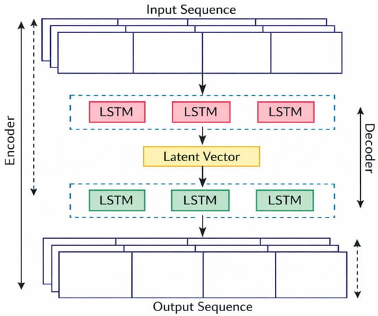
The present study employed a stacked Long Short-Term Memory (LSTM) neural network designed for the sequence-to-one time series forecasting of global and regional temperature anomalies (Figure 1). The selection of the LSTM architecture was motivated by its proven ability to capture long-range temporal dependencies and non-linear dynamics in sequential data, which are characteristic of climate processes. Unlike conventional statistical models that rely on fixed lag structures, LSTM networks utilise gated memory cells to retain relevant historical information while mitigating issues related to vanishing or exploding gradients.
Figure 1.
The conceptual architecture of the stacked LSTM forecasting model used for temperature prediction.
The model architecture consists of stacked LSTM layers followed by a fully connected output layer for temperature prediction. Input sequences were constructed using sliding windows of historical temperature observations, enabling the network to learn temporal patterns across multiple seasonals and interannual cycles. The stacked LSTM configuration enhances the model’s representational capacity by allowing higher-level temporal abstractions to be learned in deeper layers. During hyperparameter optimisation, Optuna explored ranges including 32–128 LSTM units, dropout rates between 0.1 and 0.5, learning rates between 0.0001 and 0.01, and batch sizes between 16 and 64.
The final dense layer maps the learned temporal features to continuous temperature anomaly predictions. This architecture supports the effective modelling of both trend and seasonal variability while maintaining flexibility to represent non-linear relationships. Model implementation was carried out using TensorFlow/Keras, which provides robust support for sequence modelling, hyperparameter tuning, and the efficient training of deep learning architectures. This design enhances the model’s capacity for generalisation and its ability to detect anomalies in historical climate patterns [28]. Implementation was carried out using TensorFlow/Keras due to its flexibility and support for model customisation.
3.9.2. Early Stopping
To mitigate overfitting, early stopping was employed as a regularisation strategy. During training, the model’s validation loss was monitored at the end of each epoch, and the process was terminated if no improvement was observed over a predefined patience interval. This approach reduces the likelihood of overfitting to training data while ensuring the model retains strong generalisation capability [29]. Early stopping has proven particularly effective in complex neural architectures and large-scale datasets, where it also lowers computational costs by avoiding redundant training epochs. Its effectiveness has been well documented in the literature, and practical implementations are available in deep learning frameworks such as Keras and PyTorch in Python 3.13 [30].
3.9.3. Optuna Hyperparameterisation
Hyperparameter optimisation was conducted using Optuna, an open-source framework for automated search. In contrast to traditional approaches such as grid search or random search, Optuna applies advanced algorithms, including the Tree-structured Parzen Estimator (TPE), to efficiently explore the hyperparameter space and identify optimal configurations [31]. The integration of Optuna with early stopping provided a robust training pipeline that balanced computational efficiency with predictive performance, ensuring that the developed models were both accurate and cost-effective.
3.10. Training Process
Distinct training strategies were adopted for global and regional datasets to account for their specific temporal and spatial properties. For global temperature analysis, the model was trained on the period 1766–1990 in order to capture long-term climatic trends, seasonal cycles, and historical variability across multiple centuries. Validation was performed on the subsequent period (1991–1998), which was not included in training, allowing the model to be evaluated on more recent observations and to assess its ability to generalise to modern climate conditions. For global analysis, data from 1766 to 1990 were used for model training, while observations from 1991 to 1998 were reserved for validation. The validation period was excluded from training and used to evaluate generalisation performance. The variables correspond to input sequences and target values derived from the training period, while represent sequences from the validation dataset. The temporal gap between 2001 and 2008 reflects missing or incomplete regional observations in several datasets after aggregation. These years were excluded to maintain data consistency across regions.
This split enabled the model to learn from a large and diverse historical dataset and to be tested on relatively recent data that had not been seen during training [32]. The data were detrended and converted into sequences of 30 time steps, corresponding to approximately 2.5 years. The LSTM model was constructed with LSTM, dropout, and dense layers and trained with the Adam optimiser. Early stopping was used to reduce overfitting, and Optuna was used to optimise key hyperparameters, including the number of LSTM units, dropout rates, and learning rates. These adjustments ensured that the model could capture the complex patterns of global temperature variation while maintaining stable convergence and generalisation.
For regional analysis, the training period extended from 1743 to 2000, covering pre-industrial, industrial, and modern warming phases. Validation was carried out using data from 2009 to 2013 to assess the model’s ability to generalise to more contemporary climate patterns [32]. Region-specific models were trained on 30-step sequences derived from each dataset. Optuna was again employed to optimise hyperparameters, including unit size, batch size, and learning rate, while early stopping and the Adam optimiser were consistently applied. Tailored configurations enabled localised models to achieve balanced performance, with smaller batch sizes enhancing stability in regions with limited data and optimised learning rates supporting precise convergence.
The LSTM model was trained using supervised learning on the prepared input–output sequences. Training was conducted for 50 epochs with a batch size of 32. A held-out validation set was used during training to monitor convergence and assess generalisation performance. The training process recorded loss values at each epoch, enabling the inspection of learning dynamics and potential overfitting. Model fitting was performed using the training data (X_”train” ⓜ,y_”train”), while validation was carried out on (X_”test” ⓜ,y_”test”). All key training parameters, including the number of epochs and batch size, are explicitly reported to support methodological transparency and reproducibility
3.11. Prediction, Evaluation, and Visualisation
Predictions were first generated from the residual components of the time series and subsequently reintegrated with the trend and seasonal components. This step restored the outputs to their original scale, ensuring that the results remained interpretable and consistent with real-world observations. Model performance was evaluated using standard regression metrics commonly applied in time series forecasting. Specifically, the Root Mean Squared Error (RMSE) and Mean Absolute Error (MAE) were used to quantify the magnitude of prediction errors, while the coefficient of determination (R2) measured the proportion of variance in the observed temperature series explained by the model. These metrics provide a robust assessment of forecasting accuracy and enable a direct comparison between the LSTM and SARIMA models. In addition to quantitative evaluation, graphical visualisations were used to assess model behaviour. Actual versus predicted plots illustrated the alignment between observed and forecasted temperatures at both the global and regional levels, while loss curves depicting training and validation losses across epochs provided insight into convergence behaviour and potential overfitting or underfitting.
3.12. Traditional Model Comparison
To benchmark the predictive performance of the Long Short-Term Memory (LSTM) architecture, the Seasonal Autoregressive Integrated Moving Average (SARIMA) model was employed as the primary statistical baseline. SARIMA was selected due to its established status as a standard methodology for modelling univariate time series data characterised by both trend and seasonal patterns. By incorporating autoregressive (p), differencing (d), and moving average (q) components, along with their seasonal counterparts (P, D, Q, s), SARIMA explicitly captures temporal autocorrelation structures and recurring seasonal dynamics [33].
The inclusion of SARIMA as a baseline provides a principled point of reference for assessing whether the increased model complexity and computational demands of a deep learning-based approach yield a statistically meaningful improvement in forecasting performance. To ensure a fair and systematic comparison, both the SARIMA and LSTM models were evaluated using an identical set of performance metrics, namely the Root Mean Squared Error (RMSE), Mean Absolute Error (MAE), and the coefficient of determination (R2) [34].
This comparative evaluation facilitates a direct assessment of the strengths and limitations of each modelling paradigm, contrasting the lag-based, linear structure of the SARIMA framework with the memory-based, non-linear representation learning of the LSTM model. In particular, the analysis focuses on each model’s capacity to capture the complex, non-linear dynamics inherent in global temperature anomaly time series. The SARIMA parameters (p, d, q) and seasonal parameters (P, D, Q, s) were selected using a combination of autocorrelation (ACF) and partial autocorrelation (PACF) analysis together with Akaike Information Criterion (AIC) minimisation.
3.13. Greenhouse Gas Emissions and Temperature Analysis
Following the preprocessing procedures described earlier, the temperature and emission datasets were combined to examine the role of greenhouse gas emissions in shaping climate dynamics. Three complementary analyses were conducted to provide a comprehensive perspective. A joint analysis of emission and temperature trends was carried out using dual-axis plots, with average emissions (Mt CO2 eq per year) plotted alongside average temperatures (°C). This visual approach facilitated the identification of alignments between rising emissions and temperature increases, particularly in regions characterised by intensive industrial and transportation activity. Major sectors, including agriculture, industry, and transportation, were then disaggregated into emissions. Sectoral averages were calculated and visualised to identify dominant contributors across regions. This analysis provided insights into sector-specific trajectories over time and offered evidence for targeted climate policies and mitigation strategies. Finally, a correlation analysis was conducted to evaluate the relationship between emissions and temperature variation. Pearson correlation coefficients were computed for each region using the annual averages of both variables. The resulting correlation matrices quantified the strength and direction of associations, highlighting regional differences in the influence of human activity on climate variability. It is important to note that emission data were not used as input variables for the forecasting models. Instead, they were analysed separately to explore their statistical relationship with regional temperature trends and to provide a contextual interpretation of the observed climate patterns.
4. Results
The results are organised into three components: global temperature analysis, regional forecasts, and the integration of greenhouse gas emissions with climate data. Collectively, these findings address the research objectives by tracing historical climate trends, evaluating the predictive capacity of advanced models, and linking sectoral emissions to temperature change.
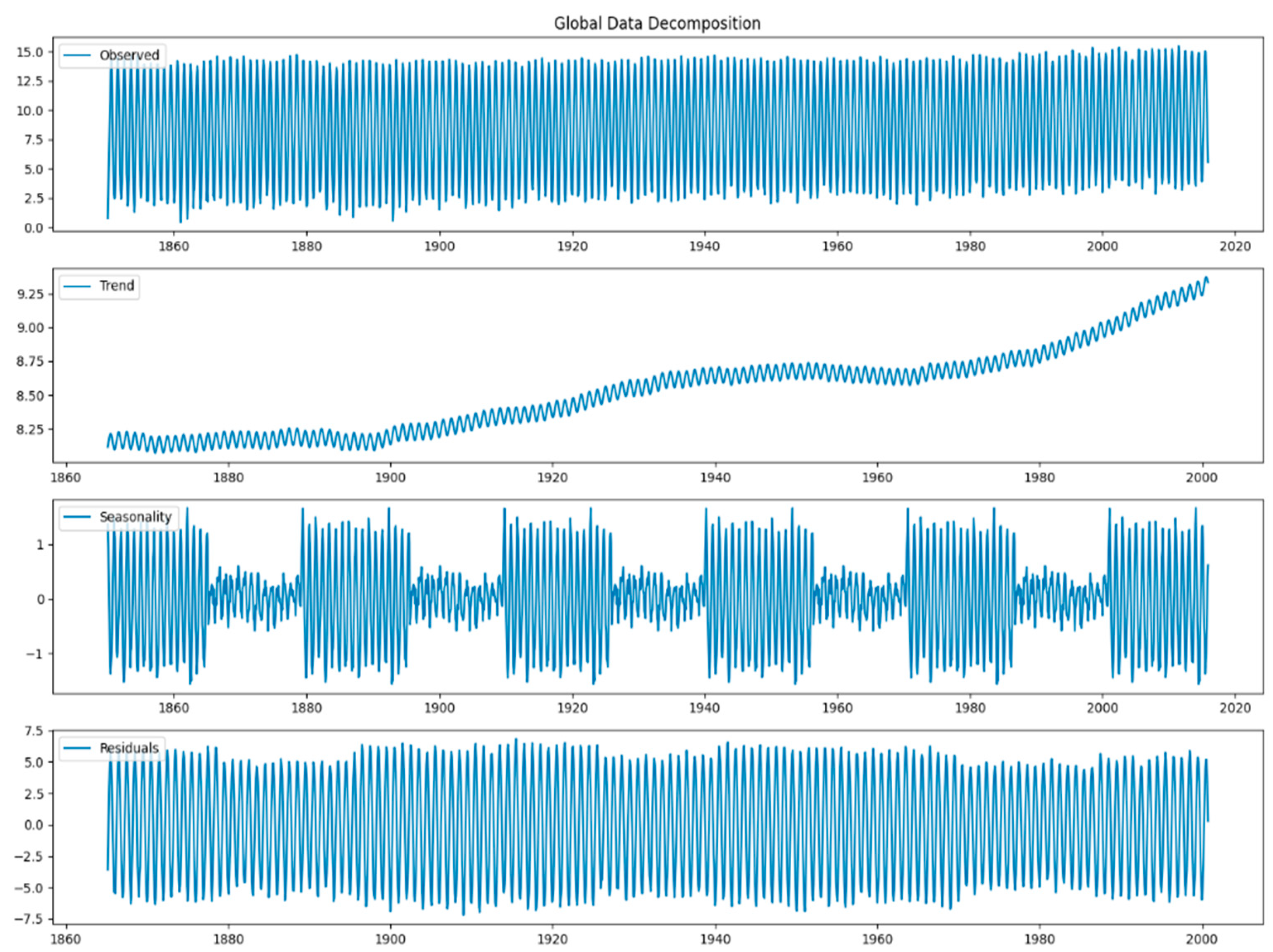
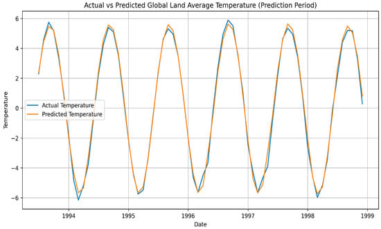
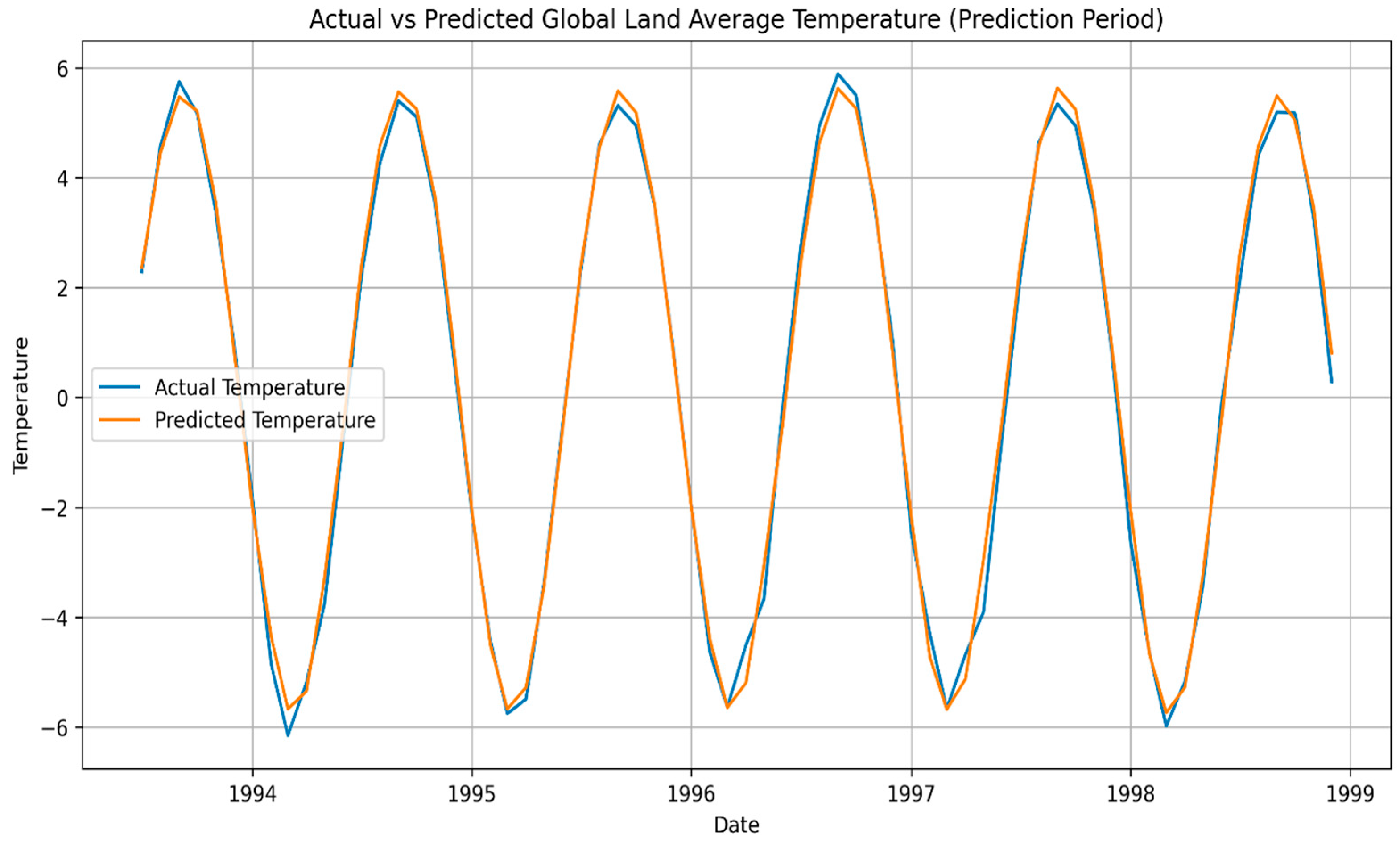
The global analysis began with the decomposition of the temperature series into trend, seasonal, and residual components. Data from 1850 to 2016 revealed annual fluctuations with stable seasonal cycles and a persistent long-term warming trajectory. The trend was relatively flat until the early twentieth century, followed by a pronounced rise coinciding with industrial expansion and increased emissions. The residual component captured short-term anomalies that intensified in recent decades, indicating growing variability in the climate system (Figure 2). The predictions generated by the LSTM model closely matched observed values, capturing both seasonal cycles and the long-term upward trend.
Figure 2.
Global data decomposition plot.
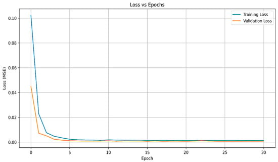
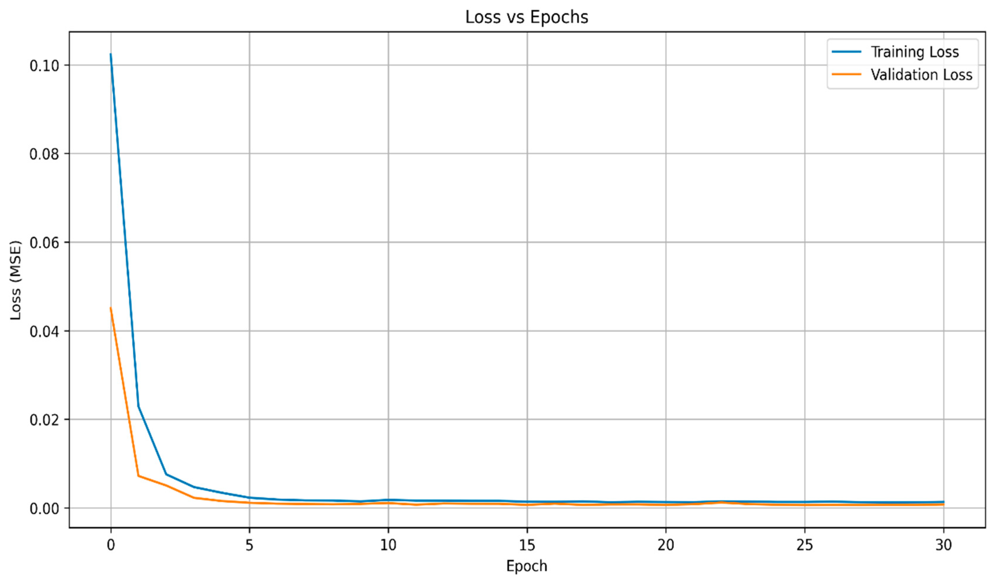
Only minor deviations occurred at extreme values, likely due to noise or external factors. Training and validation loss curves stabilised rapidly, confirming efficient learning and the absence of overfitting (Figure 3).
Figure 3.
Global data—actual vs. prediction temperature plot.
In terms of quantitative performance, the proposed LSTM model substantially outperformed the SARIMA baseline across all evaluated regression metrics, as shown in Figure 4 and Table 3. The LSTM model achieved a markedly lower Root Mean Squared Error (RMSE) of 0.1528 compared to 0.3100 for SARIMA, along with a reduced Mean Absolute Error (MAE) of 0.1198 versus 0.2653. In addition, the coefficient of determination (R2) increased from 0.9364 for the SARIMA model to 0.9846 for LSTM, indicating a stronger ability to explain variance in global temperature anomalies. Model performance was evaluated using the RMSE, MAE, and R2 to assess prediction error and goodness of fit.
Figure 4.
Global data—training and validation loss.
Table 3.
Performance metrics for global data analysis.
These results indicate that LSTM more effectively captures the temporal dependencies and non-linear dynamics present in global-scale climate time series data than the traditional SARIMA approach.
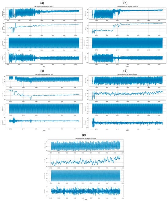
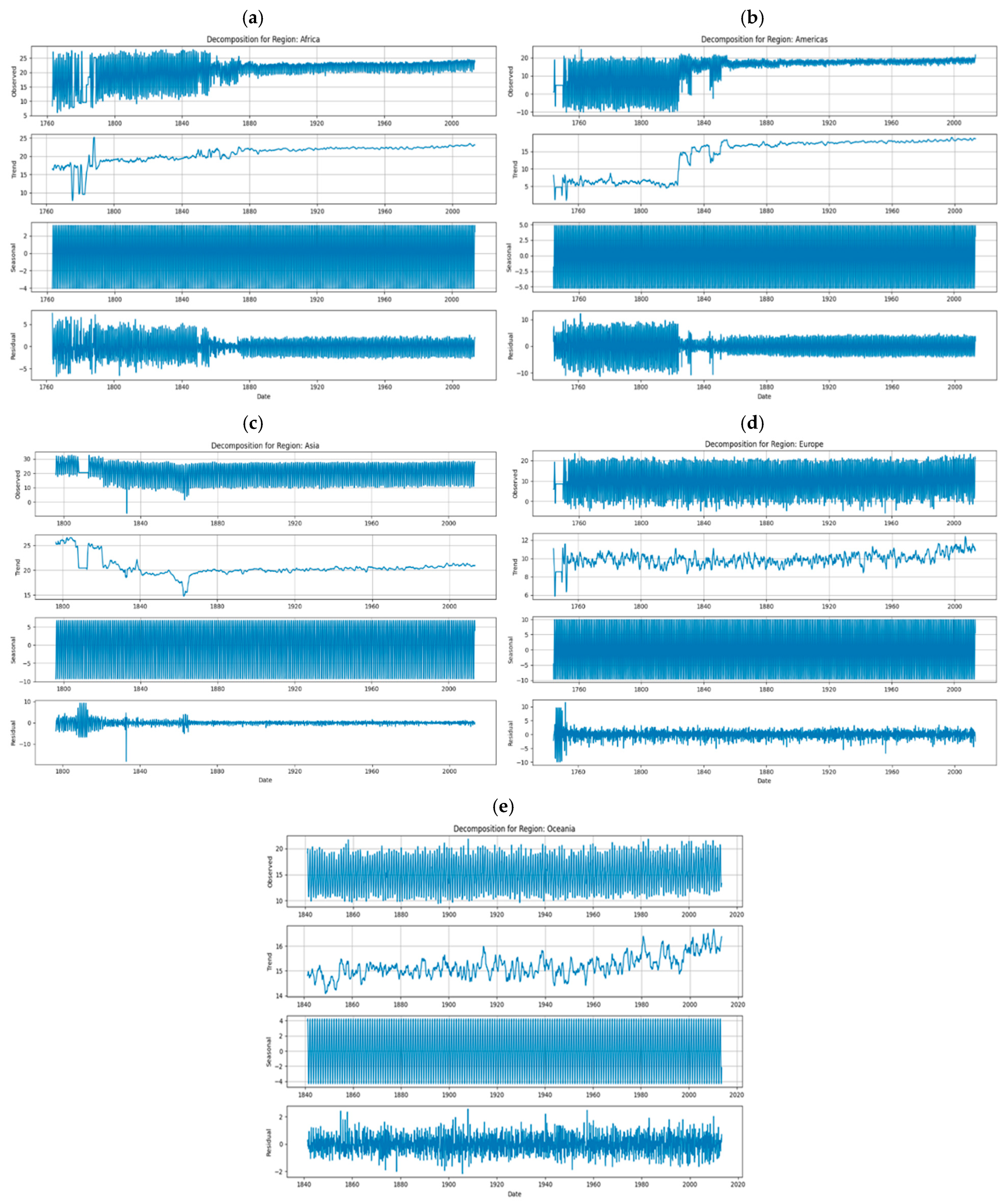
Regional analyses revealed a more heterogeneous picture (Figure 5). Africa displayed strong seasonal fluctuations and a clear twentieth-century warming signal, though residual variability was high in early years. The Americas showed consistent cycles with a rising trend, while Asia exhibited nineteenth-century anomalies followed by marked warming linked to industrialisation. Europe maintained stable seasonal cycles but experienced sharp warming after 1950. Oceania reflected steady seasonal cycles alongside anomalies associated with oceanic processes such as El Niño and La Niña.
Figure 5.
Decomposition plots for (a) Africa, (b) the Americas, (c) Asia, (d) Europe, and (e) Oceania.
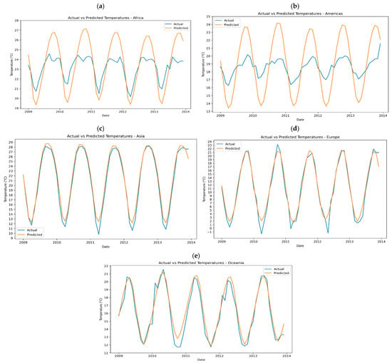
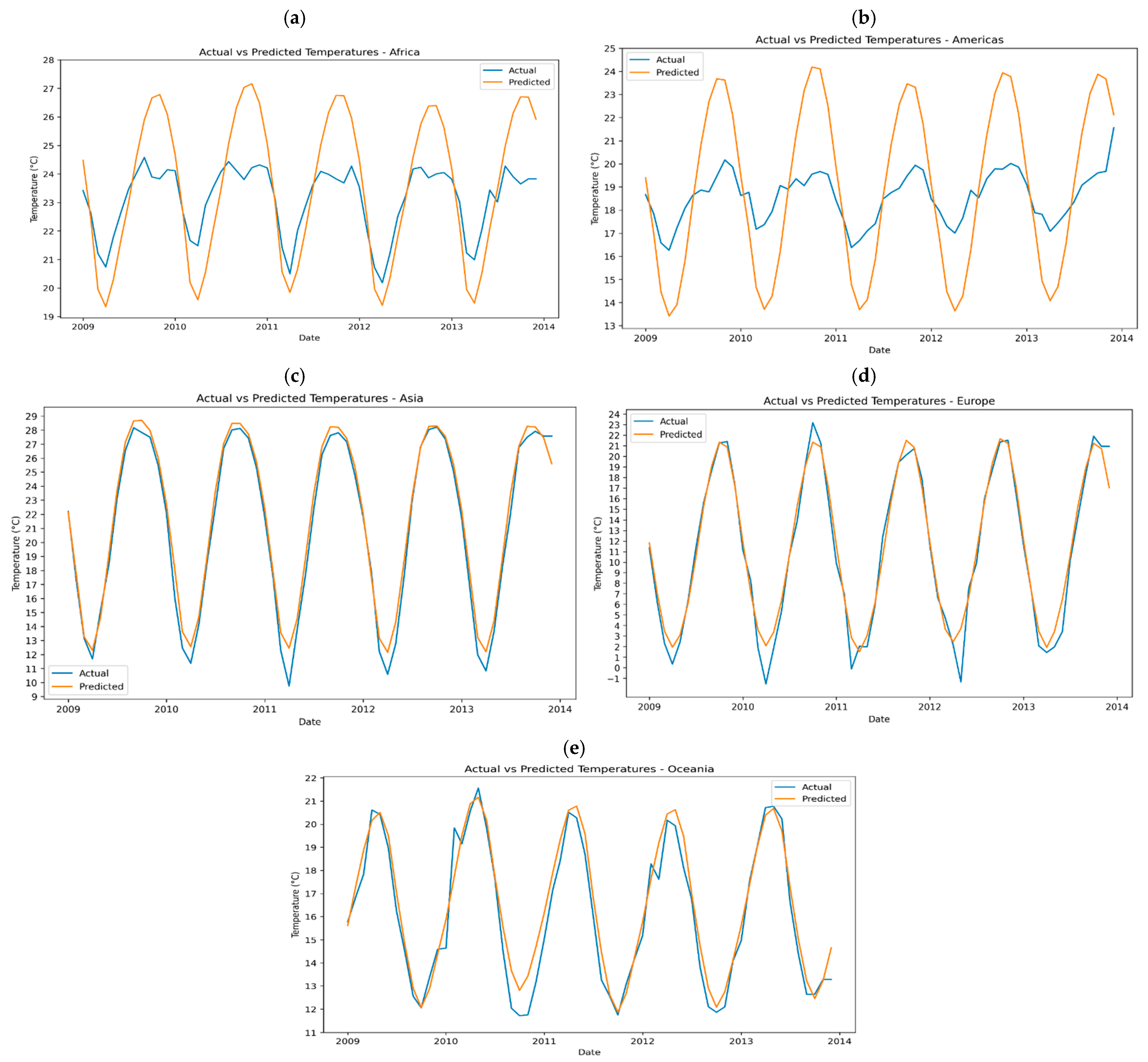
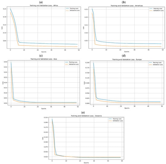
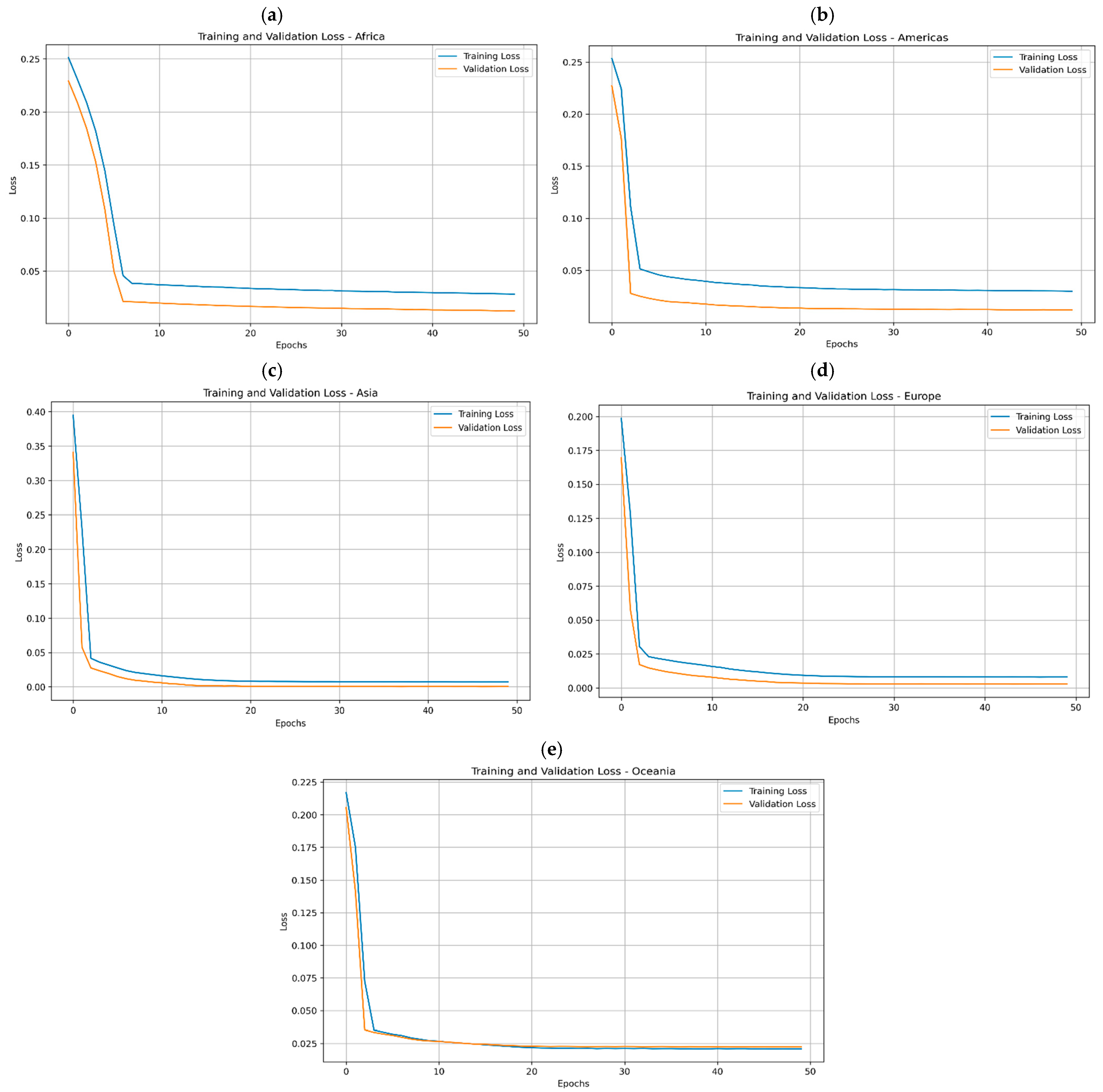
When comparing actual and predicted temperatures, regional performance varied (Figure 6). In Africa and the Americas, the model tended to exaggerate seasonal amplitudes, indicating challenges in generalising beyond cyclical patterns. Asia and Europe were modelled more accurately, with close alignment between observed and predicted series. Oceania was reasonably well captured, although amplitudes were slightly misrepresented, reflecting the strong influence of ocean-driven variability. Loss-versus-epoch plots further confirmed these observations: while Africa and the Americas showed slightly higher residual losses, Asia and Europe demonstrated smooth convergence, and Oceania exhibited stable alignment between training and validation losses (Figure 7).
Figure 6.
A comparison of actual and predicted temperatures for (a) Africa, (b) the Americas, (c) Asia, (d) Europe, and (e) Oceania.
Figure 7.
Loss vs. epochs for (a) Africa, (b) the Americas, (c) Asia, (d) Europe, and (e) Oceania.
Performance metrics revealed substantial regional variability in the predictive behaviour of the LSTM model. Although LSTM demonstrated strong performance at the global scale, its regional prediction errors were uneven. In Africa and the Americas, higher error magnitudes indicate a reduced ability to capture localised temporal dynamics. In contrast, improved performance was observed in Asia, where lower prediction errors and stronger goodness of fit suggest a closer alignment between predicted and observed temperature anomalies.
Moderate performance was evident in Europe and Oceania, where error levels remained relatively low but still reflected some degradation compared to global estimates. Overall, these findings indicate that while the LSTM model effectively captures large-scale climate dynamics, its capacity to generalise across geographically heterogeneous regions is variable, highlighting challenges associated with regional climate complexity and data heterogeneity.
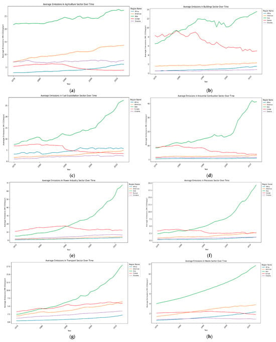
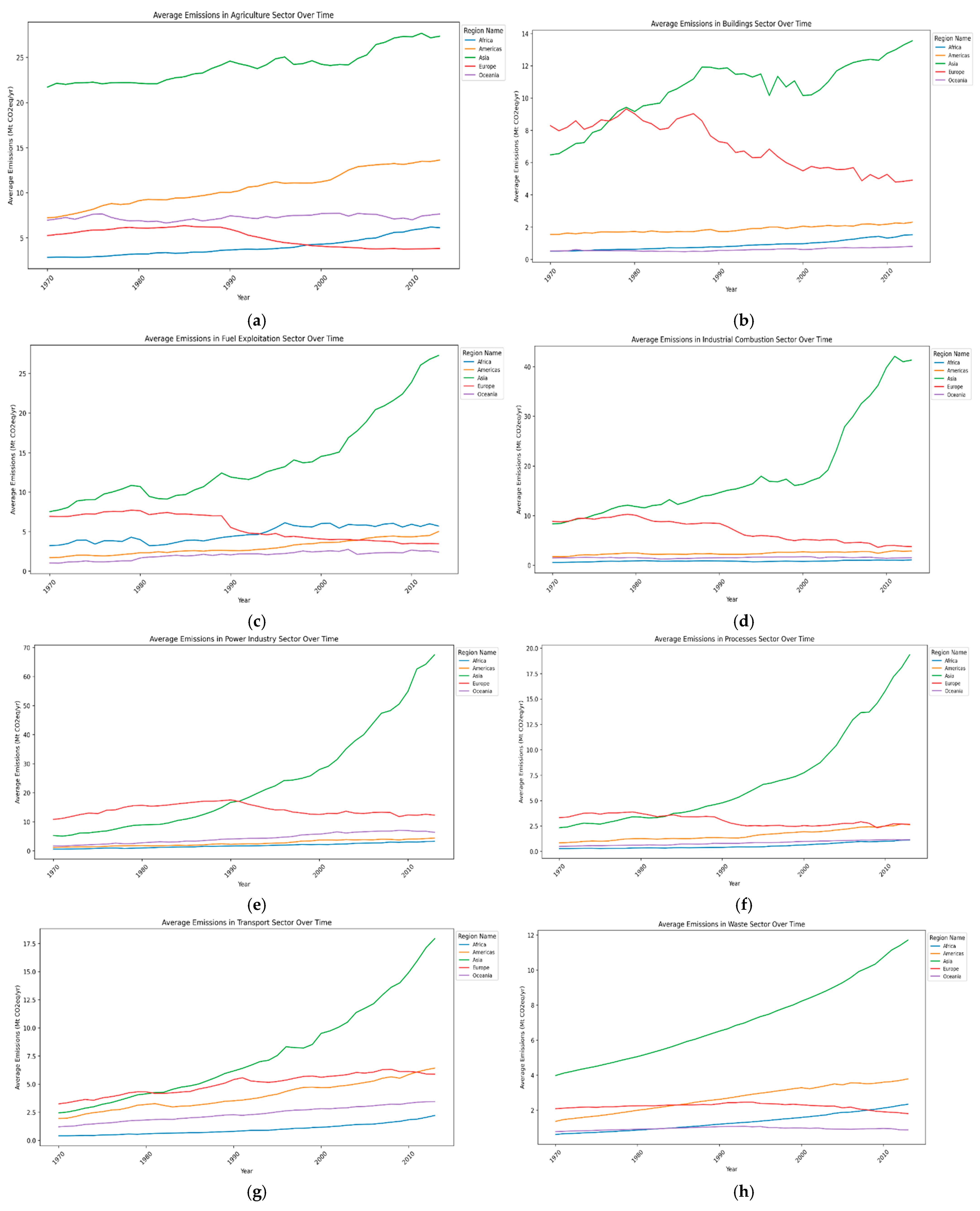
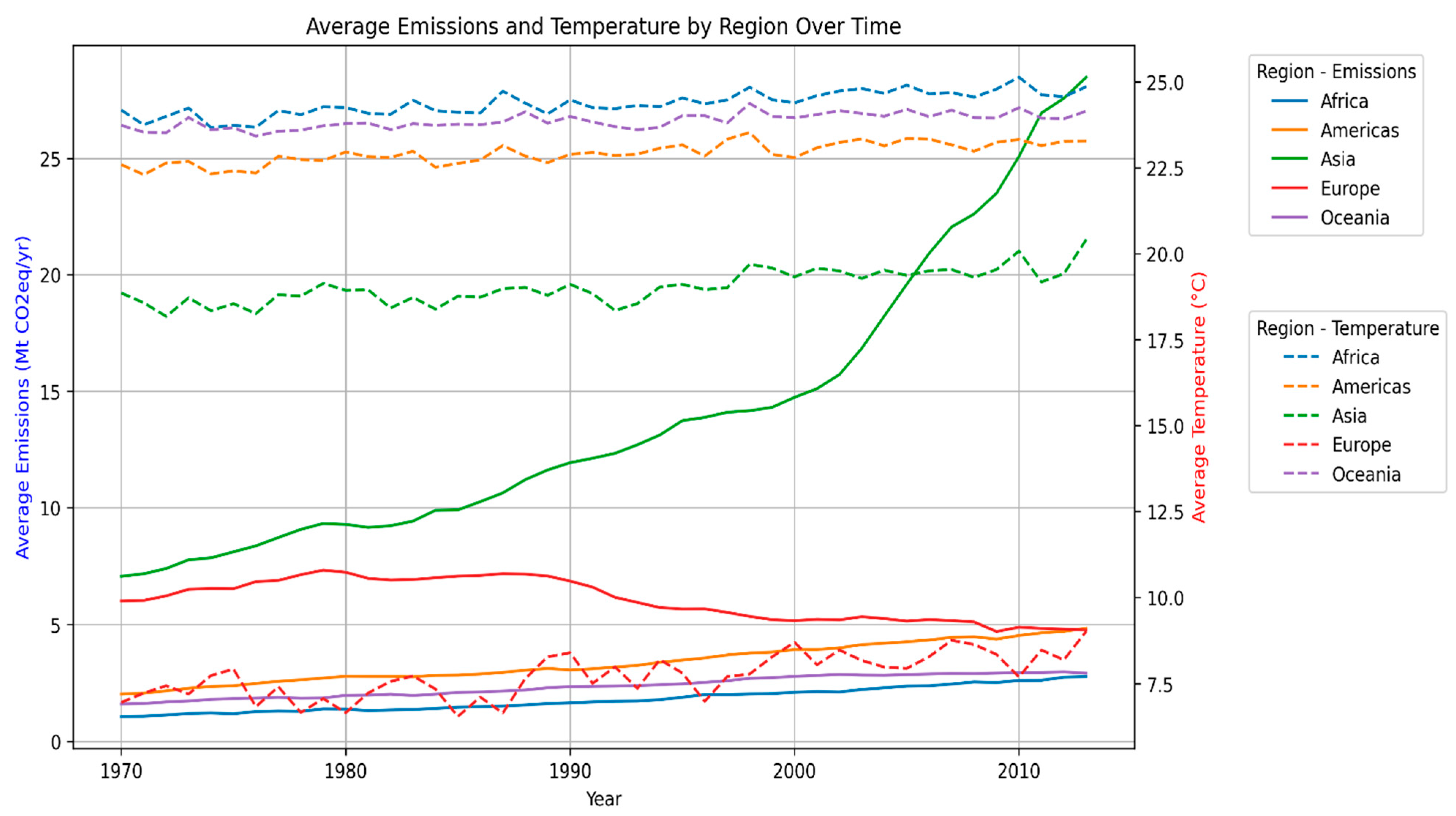
The integration of greenhouse gas emission data provided further insights (Figure 8). Across all regions, emissions rose in parallel with increasing temperatures. Asia recorded the steepest rise since the 1990s, while Europe’s emissions declined, but temperatures continued to rise, reflecting the delayed impacts of past accumulation. Africa and Oceania, despite their low emissions, experienced comparable warming trends, underscoring the global nature of climate change.
Figure 8.
Average emissions over time by sector: (a) agriculture, (b) buildings, (c) fuel exploitation, (d) industrial combustion, (e) power industry, (f) processes, (g) transport, (h) waste.
Sectoral analysis highlighted regional contrasts (Figure 9). In Asia, the power sector and industrial combustion accounted for the majority of emissions, whereas agriculture was more influential in Africa and the Americas. Europe reduced emissions from power and industry but retained substantial contributions from agriculture and transport. Oceania’s emissions were lower overall yet broadly distributed across sectors.
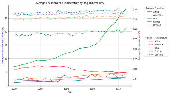
Figure 9.
Average emissions and temperatures by region overtime.
Correlation analysis supported these findings, revealing strong positive relationships between industrial and energy-related emissions and warming in Asia and highlighting the role of agricultural emissions in Africa and the Americas. In Europe, agriculture and transport remained correlated with rising temperatures despite reductions in total emissions, while Oceania exhibited weaker but more evenly distributed sectoral correlations (Table 4).
Table 4.
Regional trends in average waste sector emissions (Mt CO2 eq/yr, 1970–2010).
In summary, the results confirm that the LSTM architecture effectively models global climate dynamics, significantly outperforming the SARIMA statistical framework on a global scale. At the regional level, however, performance was notably uneven; the SARIMA model and simpler linear baselines often provided more stable results, particularly in regions where LSTM exhibited high-amplitude variance. The inclusion of emission data validated the central role of anthropogenic activity while emphasising sectoral and regional differences, highlighting the importance of context-specific strategies for climate mitigation.
5. Discussion
The outcomes of this study provide an integrated assessment of the role of advanced deep learning methods in climate forecasting, with a particular emphasis on the LSTM model. By combining global and regional temperature predictions with greenhouse gas emission analysis, this research offers both methodological and practical insights into the drivers of climate variability and the suitability of different modelling approaches.
At the global scale, the LSTM model clearly outperformed traditional methods such as SARIMA. The model captured long-term warming trends, seasonal cycles, and residual anomalies with high fidelity, supported by strong quantitative metrics and the stable convergence of training and validation losses. These results highlight the strength of recurrent neural networks in modelling sequential dependencies across extended historical datasets. They also confirm the findings in the existing literature, which emphasise the ability of deep learning to capture non-linear relationships and detect complex patterns that more conventional models often miss. Such capacity is crucial for global climate datasets, where variability arises not only from natural processes but also from human-induced change across centuries.
However, regional analyses revealed that performance is not uniform. LSTM achieved strong results in Asia, Europe, and Oceania but performed less reliably in Africa and the Americas. Several factors may explain this discrepancy. First, data quality and availability vary considerably between regions. In Africa, gaps in historical data and variability in measurement practices likely contributed to higher residual errors and exaggerated prediction amplitudes. In the Americas, the sheer diversity of climate zones, stretching from tropical to polar, may have posed challenges for the model’s ability to generalise seasonal and long-term patterns. In contrast, Asia and Europe offered more extensive and consistent datasets, enabling LSTM to identify long-term dependencies more effectively. Oceania’s results, although less precise in amplitude, demonstrated that the model could still account for ocean-driven anomalies, reflecting its flexibility in capturing diverse climatic signals.
These findings suggest that deep learning models cannot be viewed as universally superior to traditional approaches. While they excel at detecting complex global-scale dynamics, simpler ensemble or regression methods may outperform them in contexts where datasets are noisy, sparse, or regionally heterogeneous. This emphasises the need for a context-sensitive approach to climate modelling, in which model selection is tailored to the dataset’s characteristics and the research objective. Hybrid frameworks that combine neural networks with traditional models may therefore provide the most effective solution, balancing predictive accuracy with robustness in data-limited settings.
The inclusion of emission data added a crucial socio-economic perspective to the analysis. Across all regions, emissions rose in parallel with temperature increases, although the magnitude and timing varied. Asia showed the strongest link, with industrialisation and fossil fuel dependence driving rapid increases in both emissions and temperatures since the 1990s. Europe, by contrast, exhibited declining emissions but continued warming, highlighting the cumulative and lagging effects of historical greenhouse gas accumulation. Africa and Oceania demonstrated that even regions with relatively low emissions experience warming, reflecting the global interconnectedness of climate processes.
Sectoral analysis further underscored regional differences. Agriculture emerged as a key contributor in Africa and the Americas, linked to land-use practices and livestock production, while energy and industrial combustion dominated in Asia. Europe displayed declines in several sectors due to climate policies and transitions toward renewables, though agriculture and transport remained persistent sources. Oceania’s emissions were lower but more evenly distributed across sectors, reflecting its unique socio-economic profile. Correlation analyses confirmed these patterns, showing strong statistical associations between sector-specific emissions and temperature increases, with regional variation.
Despite the promising results, several sources of uncertainty should be acknowledged. Regional datasets vary in spatial coverage and historical measurement consistency, which may influence model performance in data-sparse regions such as parts of Africa and the Americas. In addition, missing values were handled through forward-fill imputation, which may introduce smoothing effects in long historical records. Model performance may also be sensitive to the chosen sequence length (30-month window), which determines the temporal context available for prediction. These findings are consistent with previous studies showing that deep learning models such as LSTM can capture long-term temporal dependencies in climate data, while traditional statistical models may provide more stable performance in data-limited regional contexts.
Taken together, the results illustrate that deep learning models can provide valuable insights into global climate trends but must be applied with caution at the regional level. They also emphasise the importance of integrating socio-economic data into predictive frameworks, as emission patterns reveal the human drivers behind observed warming and highlight opportunities for targeted interventions.
6. Conclusions and Future Work
This study investigated the use of a stacked LSTM forecasting model to forecast global and regional temperature changes and explored the link between greenhouse gas emissions and climate variability. The results demonstrate that while advanced deep learning techniques offer significant advantages over traditional models, particularly at the global level, their effectiveness at the regional scale is shaped by data availability, quality, and climatic diversity.
At the global level, the LSTM model captured long-term warming trends, seasonal cycles, and anomalies effectively and achieved higher predictive accuracy than the SARIMA baseline. Its strong predictive performance underscores the potential of deep learning to advance climate science by modelling non-linear dynamics and long temporal dependencies. These findings suggest that deep learning can contribute meaningfully to global climate forecasting and help refine projections that inform international climate agreements and strategies.
The regional findings, however, reveal the limits of deep learning in heterogeneous contexts. In Africa and the Americas, traditional models often outperformed the LSTM model, reflecting the challenges posed by incomplete data and diverse climate systems. This indicates that model selection should not follow a one-size-fits-all approach but rather adapt to the analysis’s context. Hybrid modelling frameworks that combine the strengths of deep learning with the robustness of traditional methods may be particularly valuable for regional forecasting.
The integration of emission data added a socio-economic layer to the analysis, confirming strong correlations between human activity and warming. Agriculture, power generation, and industry emerged as the most significant global contributors; however, their relative importance varied by region. These results offer policy-relevant insights, highlighting where mitigation strategies may be the most effective. For instance, reforms in agricultural practices could be prioritised in Africa and the Americas, while reductions in energy-related emissions are the most urgent in Asia. Europe’s continued warming despite declining emissions underscores the inertia of the climate system and the need for long-term, sustained action.
In regions such as Africa and parts of the Americas, historical temperature records are comparatively sparse and unevenly distributed across time and geography. This data sparsity can limit the ability of deep learning models to learn stable temporal representations. In such contexts, simpler statistical models with fewer parameters may sometimes produce more stable predictions because they rely on stronger structural assumptions and require less data for effective calibration.
Despite its contributions, this study faces limitations. The LSTM model’s underperformance in some regions underscores the need for more comprehensive, higher-quality data. The absence of additional socio-economic indicators, such as population dynamics, technology adoption, and policy measures, limited the explanatory scope of the emission analysis. Including these variables would enable a more holistic understanding of the relationship between human activity and climate outcomes.
Future work should focus on four primary areas. First, expanding the dataset to include more recent observations and additional climate variables, such as precipitation and atmospheric pressure, would improve predictive accuracy. Second, developing hybrid models that integrate deep learning with traditional approaches could improve robustness across regions. Third, incorporating socio-economic indicators alongside emission data would provide a more comprehensive framework for linking human activity to climate outcomes. Finally, enhancing the interpretability of deep learning models is essential for building trust among policymakers and researchers, ensuring that advanced methods are not only accurate but also transparent.
In conclusion, this research demonstrates the promise and limitations of LSTM models in climate forecasting. While highly effective at the global scale, their regional application requires the careful consideration of data quality and context. By combining predictive modelling with emission analysis, this study contributes to a more complete understanding of climate dynamics and provides insights that are directly relevant to policy and mitigation strategies. Ultimately, the findings highlight the importance of global collaboration coupled with region-specific approaches, ensuring that scientific advances are translated into actionable solutions for addressing climate change.
Author Contributions
Conceptualization, A.N.G.R., N.S. and P.S.; methodology, A.N.G.R., N.S. and P.S.; software, A.N.G.R.; validation, A.N.G.R.; writing—original draft preparation, A.N.G.R., N.S. and P.S.; writing—review and editing, N.S. and P.S.; supervision, N.S. and P.S. All authors have read and agreed to the published version of the manuscript.
Funding
This research received no external funding.
Data Availability Statement
The temperature datasets used in this study are publicly available from the Berkeley Earth dataset. Greenhouse gas emission data were obtained from the EDGAR database. All datasets used in this study are publicly accessible through their respective repositories.
Acknowledgments
This paper is based on the author’s unpublished Master’s thesis entitled Analysing and Modelling Historical Global and Regional Temperature Shifts Using Deep Learning Techniques and Greenhouse Gas Emissions Analysis, submitted in partial fulfilment of the requirements for a Master’s degree at Dalarna University, Borlänge, Sweden, on 15 January 2025. The thesis was conducted under the supervision of Paria Sadeghian and Nausheen Saeed. The author Arambage Navodya Gimhani Ranasinghe gratefully acknowledges their invaluable guidance, constructive feedback, and continuous academic support throughout the research process. Their expertise and encouragement were instrumental in shaping the direction, methodology, and overall quality of this work.
Conflicts of Interest
The authors declare no conflict of interest.
References
- Bormashenko, E. What is temperature? Modern outlook on the concept of temperature. Entropy 2020, 22, 1366. [Google Scholar] [CrossRef] [Scilit] [PubMed]
- Chang, H. Inventing Temperature: Measurement and Scientific Progress; Oxford Academic: New York, NY, USA, 2005. [Google Scholar] [CrossRef] [Scilit]
- Hansen, J.; Ruedy, R.; Sato, M.; Lo, K. Global surface temperature change. Rev. Geophys. 2010, 48, RG4004. [Google Scholar] [CrossRef] [Scilit]
- Masson-Delmotte, V. Climate Change 2021: The Physical Science Basis: Working Group I Contribution to the Sixth Assessment Report of the Intergovernmental Panel on Climate Change; IPCC: Geneva, Switzerland, 2023. [Google Scholar]
- Lockwood, M.; Fröhlich, C. Recent oppositely directed trends in solar climate forcings and the global mean surface air temperature. Proc. R. Soc. A Math. Phys. Eng. Sci. 2007, 463, 2447–2460. [Google Scholar] [CrossRef] [Scilit]
- Robock, A. Volcanic eruptions and climate. Rev. Geophys. 2000, 38, 191–219, Erratum in Rev. Geophys. 2007, 45, RG3005. [Google Scholar] [CrossRef] [Scilit]
- Berger, A.L. Long-term variations of daily insolation and Quaternary climatic changes. J. Atmos. Sci. 1978, 35, 2361–2367. [Google Scholar] [CrossRef] [Scilit]
- Marshall, J.; Speer, K. Closure of the meridional overturning circulation through Southern Ocean upwelling. Nat. Geosci. 2012, 5, 171–180. [Google Scholar] [CrossRef] [Scilit]
- Sadeghian, P.; Golshan, A.; Zhao, M.; Håkansson, J. A Deep Semi-Supervised Machine Learning Algorithm for Detecting Transportation Modes Based on Gps Tracking Data. SSRN Electron. J. 2022. [Google Scholar] [CrossRef] [Scilit]
- Saeed, N.; Alam, M.; Nyberg, R.G.; Dougherty, M.; Jomaa, D.; Rebreyend, P. Comparison of Pattern Recognition Techniques for Classification of the Acoustics of Loose Gravel. In Proceedings of the 2020 7th IEEE International Conference on Soft Computing & Machine Intelligence (ISCMI); Stockholm, Sweden, 14–15 November 2020, IEEE: Piscataway, NJ, USA, 2020; pp. 237–243. [Google Scholar] [CrossRef] [Scilit]
- Berner, R.A. Atmospheric oxygen over Phanerozoic time. Proc. Natl. Acad. Sci. USA 1999, 96, 10955–10957. [Google Scholar] [CrossRef] [Scilit] [PubMed]
- Intergovernmental Panel on Climate Change (IPCC). Human Influence on the Climate System. In Climate Change 2021—The Physical Science Basis; Cambridge University Press: Cambridge, UK, 2023; pp. 423–552. [Google Scholar] [CrossRef] [Scilit]
- Omer, A.M. Energy, environment and sustainable development. Renew. Sustain. Energy Rev. 2008, 12, 2265–2300. [Google Scholar] [CrossRef] [Scilit]
- Johnson, S.J.; Stockdale, T.N.; Ferranti, L.; Balmaseda, M.A.; Molteni, F.; Magnusson, L.; Tietsche, S.; Decremer, D.; Weisheimer, A.; Balsamo, G.; et al. SEAS5: The new ECMWF seasonal forecast system. Geosci. Model Dev. 2019, 12, 1087–1117. [Google Scholar] [CrossRef] [Scilit]
- Sadeghian, P.; Mojarrad, B.B. Analysing Gender and Temporal Dynamics in Human Mobility Patterns in Central Sweden. Geographies 2025, 5, 7. [Google Scholar] [CrossRef] [Scilit]
- Golshan, A.; Sardar, S.; Mahdavi Ardestani, S.F.; Sadeghian, P. A Fuzzy Analytical Network Process Framework for Prioritizing Competitive Intelligence in Startups. Analytics 2025, 4, 3. [Google Scholar] [CrossRef] [Scilit]
- Sadeghian, P. A Multi-Dimensional Approach to Human Mobility and Transportation Mode Detection Using GPS Data. Doctoral Dissertation, Dalarna University, Falun, Sweden, 2024. [Google Scholar]
- Weyn, J.A.; Durran, D.R.; Caruana, R. Improving Data-Driven Global Weather Prediction Using Deep Convolutional Neural Networks on a Cubed Sphere. J. Adv. Model. Earth Syst. 2020, 12, e2020MS002109. [Google Scholar] [CrossRef] [Scilit]
- El-Habil, B.Y.; Abu-Naser, S.S. Global climate prediction using deep learning. J. Theor. Appl. Inf. Technol. 2022, 100, 4824–4838. [Google Scholar]
- Hou, J.; Wang, Y.; Zhou, J.; Tian, Q. Prediction of hourly air temperature based on CNN–LSTM. Geomat. Nat. Hazards Risk 2022, 13, 1962–1986. [Google Scholar] [CrossRef] [Scilit]
- Gong, B.; Langguth, M.; Ji, Y.; Mozaffari, A.; Stadtler, S.; Mache, K.; Schultz, M.G. Temperature forecasting by deep learning methods. Geosci. Model Dev. 2022, 15, 8931–8956. [Google Scholar] [CrossRef] [Scilit]
- Hamdan, A.; Al-Salaymeh, A.; AlHamad, I.M.; Ikemba, S.; Ewim, D.R.E. Predicting future global temperature and greenhouse gas emissions via LSTM model. Sustain. Energy Res. 2023, 10, 21. [Google Scholar] [CrossRef] [Scilit]
- Malakouti, S.M. Utilizing time series data from 1961 to 2019 recorded around the world and machine learning to create a Global Temperature Change Prediction Model. Case Stud. Chem. Environ. Eng. 2023, 7, 100312. [Google Scholar] [CrossRef] [Scilit]
- Bochenek, B.; Ustrnul, Z. Machine Learning in Weather Prediction and Climate Analyses—Applications and Perspectives. Atmosphere 2022, 13, 180. [Google Scholar] [CrossRef] [Scilit]
- Gao, L.; Yang, Y.-M.; Li, Q.; Ham, Y.-G.; Kim, J.-H. Deep Learning for Predicting Winter Temperature in North China. Atmosphere 2022, 13, 702. [Google Scholar] [CrossRef] [Scilit]
- Chen, L.; Han, B.; Wang, X.; Zhao, J.; Yang, W.; Yang, Z. Machine Learning Methods in Climate Prediction: A Survey. Preprints 2023. [Google Scholar] [CrossRef]
- Edgar. EDGAR–Emission Database for Global Atmospheric Research. Global Emissions. EDGAR v4.2 (November 2011); JRC: Ispra, Italy, 2011. [Google Scholar]
- Gers, F.A.; Schmidhuber, J.; Cummins, F. Learning to forget: Continual prediction with LSTM. Neural Comput. 2000, 12, 2451–2471. [Google Scholar] [CrossRef] [Scilit]
- Bengio, Y. Practical Recommendations for Gradient-Based Training of Deep Architectures. In Neural Networks: Tricks of the Trade; Lecture Notes in Computer Science; Springer: Berlin/Heidelberg, Germany, 2012; Volume 7700, pp. 437–478. [Google Scholar]
- Lawrence, S.; Giles, L. Overfitting and neural nets: Conjugate gradient and backpropagation. In Proceedings of the IEEE-INNS-ENNS International Joint Conference on Neural Networks—IJCNN 2000, Como, Italy, 27 July 2000; IEEE: Piscataway, NJ, USA, 2000; pp. 402–408. [Google Scholar] [CrossRef] [Scilit]
- Akiba, T.; Sano, S.; Yanase, T.; Ohta, T.; Koyama, M. Optuna: A Next-generation Hyperparameter Optimization Framework. In Proceedings of the ACM SIGKDD International Conference on Knowledge Discovery and Data Mining, Anchorage, AK, USA, 3–7 August 2019; ACM: New York, NY, USA, 2019. [Google Scholar] [CrossRef] [Scilit]
- Medar, R.; Rajpurohit, V.S.; Rashmi, B. Impact of Training and Testing Data Splits on Accuracy of Time Series Forecasting in Machine Learning. In Proceedings of the 2017 International Conference on Computing, Communication, Control and Automation (ICCUBEA), Pune, India, 17–18 August 2017; IEEE: Piscataway, NJ, USA, 2017; pp. 1–6. [Google Scholar]
- Tang, C.; Tong, Z.; Wei, Y.; Wu, X.; Tian, X.; Yang, J. Time–Frequency Characteristics and SARIMA Forecasting of Atmospheric Water Vapor in East Asia. Atmosphere 2023, 14, 899. [Google Scholar] [CrossRef] [Scilit]
- Ariyanti, V.P.; Yusnitasari, T. Comparison of ARIMA and SARIMA for Forecasting Crude Oil Prices. J. RESTI 2023, 7, 405–413. [Google Scholar] [CrossRef] [Scilit]

Disclaimer/Publisher’s Note: The statements, opinions and data contained in all publications are solely those of the individual author(s) and contributor(s) and not of MDPI and/or the editor(s). MDPI and/or the editor(s) disclaim responsibility for any injury to people or property resulting from any ideas, methods, instructions or products referred to in the content. |
© 2026 by the authors. Licensee MDPI, Basel, Switzerland. This article is an open access article distributed under the terms and conditions of the Creative Commons Attribution (CC BY) license.